1 Introduction
The coupled motion of two physically distinct phases dictates a number of natural phenomena, such as the migration and storage of magma in the Earth’s mantle, the compaction of sedimentary basins, porous flow of hydrocarbon and groundwater, and the dynamics of melting of sea ice. Flow in such natural multiphase systems involves coupled conservation of mass, momentum and energy between two distinct, coexisting phases. These conservation relations arise from flow in two interconnected phases: the load-bearing, creeping matrix and the inviscid, interstitial fluid. A large body of publications studied the derivation of these coupled conservation equations, their stability, associated nonlinear phenomena, analytical and numerical solutions, and their application to various natural phenomena (e.g. Drew Reference Drew1971, Reference Drew1983; McKenzie Reference McKenzie1984; Barcilon & Lovera Reference Barcilon and Lovera1989; Spiegelman Reference Spiegelman1993a ,Reference Spiegelman b ; Bercovici, Ricard & Schubert Reference Bercovici, Ricard and Schubert2001a ,Reference Bercovici, Ricard and Schubert b ; Ricard, Bercovici & Schubert Reference Ricard, Bercovici and Schubert2001; Hier-Majumder, Ricard & Bercovici Reference Hier-Majumder, Ricard and Bercovici2006; Takei & Hier-Majumder Reference Takei and Hier-Majumder2009; Simpson, Spiegelman & Weinstein Reference Simpson, Spiegelman and Weinstein2010a ,Reference Simpson, Spiegelman and Weinstein b ; Rudge, Bercovici & Spiegelman Reference Rudge, Bercovici and Spiegelman2011; Rudge Reference Rudge2014). Based on the results of these studies and natural observations, a few facts emerge about viscous multiphase flow in nature. First, natural phenomena arising from multiphase flow can take place over a large variety of length scales. Second, many natural phenomena involve interaction between multiple domains consisting of multiphase aggregates. Such domains are often marked by contrasting effective physical properties and are separated by a distinct interface. Finally, during coupled flow of deforming multiphase aggregates, the weaker phase self-segregates during the flow. Such self-segregation of the weak phase is often the most interesting feature of natural multiphase flow, as it has strong implications for the storage, migration and stability of partial melt in the deep Earth or the effective strength of an aggregate on a microscopic scale.
One important example of coupled multiphase flow comes from recent seismic observations at the Earth’s core–mantle boundary. The Earth’s lower mantle, the bottom of the viscous, rocky layer above the metallic core, is marked by two large structures, located diametrically opposite to each other, one beneath Africa and the other beneath the Pacific Ocean (McNamara, Garnero & Rost Reference McNamara, Garnero and Rost2010). Often described as the large low-shear-velocity provinces (LLSVPs), owing to their seismic signature, these structures are compositionally distinct from the rest of the mantle, contain multiple viscous solid phases of contrasting strength, and are marked by convective flows within their interior (McNamara et al. Reference McNamara, Garnero and Rost2010; Bower et al. Reference Bower, Wicks, Gurnis and Jackson2011). The bottom edges of the LLSVPs are marked by another set of patchy, smaller structures, called ultra-low-velocity zones (ULVZs) (Williams & Garnero Reference Williams and Garnero1996; Rost & Revenaugh Reference Rost and Revenaugh2003; Rost et al. Reference Rost, Garnero, Williams and Manga2005). The location of ULVZs, also containing multiple solid and fluid phases, within the LLSVPs seems to suggest that the ULVZs are swept around and deformed by the flow within the LLSVPs (Hier-Majumder & Revenaugh Reference Hier-Majumder and Revenaugh2010; McNamara et al. Reference McNamara, Garnero and Rost2010; Bower et al. Reference Bower, Wicks, Gurnis and Jackson2011; Hier-Majumder & Drombosky Reference Hier-Majumder and Drombosky2016). The ULVZs and LLSVPs are marked by sharp boundaries separating them from the surrounding mantle. To study the distribution of the weaker phases within the ULVZs, it is therefore crucial to understand the way the flow within these two multiphase domains with distinctive average physical properties are coupled (Hier-Majumder & Revenaugh Reference Hier-Majumder and Revenaugh2010; Hier-Majumder Reference Hier-Majumder2014; Hier-Majumder & Drombosky Reference Hier-Majumder and Drombosky2016). In a recent study, Hier-Majumder & Drombosky (Reference Hier-Majumder and Drombosky2016) outlined the nature of coupled flow within these two bodies. This study modelled the flow using the boundary integral formulation of coupled Stokes flow within the ULVZ and the LLSVP. As a result, this study was unable to quantify the nature of compaction and segregation of the constituent phases.
A second example of coupled flow arises from observations on a different length scale. In the Earth’s lower crust, viscous deformation of multiphase rocks can often be associated with characteristic structures on the microscopic scale. Deformation of these rocks, consisting of several different mineral phases, leads to the establishment of pockets of multiple weak mineral phases embedded in a substrate consisting of stronger mineral phases (Handy, Wissing & Streit Reference Handy, Wissing and Streit1999; Holyoke & Tullis Reference Holyoke and Tullis2006; Qi, Zhao & Kohlstedt Reference Qi, Zhao and Kohlstedt2013). As the deformation of these rocks facilitates the motion of overlying tectonic plates, the interaction between these pockets of weakness plays an important role in establishing the effective strength of the rocks (Handy et al. Reference Handy, Wissing and Streit1999). Since both the substrate and the pockets consist of multiple phases, to understand the separation of phases within each of these domains, the nature of coupling between the two flows is quite important.
Both of these natural examples demand a theoretical construct involving multiple, interacting domains of multiphase aggregates. Often one of these domains can be characterized by substantially different average physical properties, such as shear viscosity of the load-bearing matrix. In reconstructing geological events of the past from microstructures, or to infer the nature of mantle flow from present-day seismic observations in the Earth, it is crucial to understand the influence of such contrast in physical properties between different domains on the nature of flow and phase segregation within each domain.
The interaction between viscous bodies of single-phase fluids, suspended in a single, viscous fluid phase, has been studied at length over the past several decades, building on the work of Taylor (Reference Taylor1932). These studies investigated the interaction between particles and substrates in areas including drop deformation (Pozrikidis Reference Pozrikidis1990; Manga & Stone Reference Manga and Stone1995; Li & Pozrikidis Reference Li and Pozrikidis1996), emulsions and foams (Li, Zhou & Pozrikidis Reference Li, Zhou and Pozrikidis1995; Loewenberg & Hinch Reference Loewenberg and Hinch1996), volcanology (Manga & Loewenberg Reference Manga and Loewenberg2001; Rust & Manga Reference Rust and Manga2002), rheology (Taylor Reference Taylor1932; Li & Pozrikidis Reference Li and Pozrikidis1997; Manga et al. Reference Manga, Castro, Cashman and Loewenberg1998) and microstructure in sintering materials (Hopper Reference Hopper1993a ,Reference Hopper b ; Kuiken Reference Kuiken1993; Hier-Majumder Reference Hier-Majumder2008, Reference Hier-Majumder2011; Hier-Majumder & Abbott Reference Hier-Majumder and Abbott2010). The governing equations for these studies involve Stokes flow within two domains, the suspended drop and the medium of suspension. The conservation of mass and momentum for Stokes flow is supplemented by a set of boundary conditions, typically continuity of velocity and balance of traction, often with a constant or spatially varying surface tension at the interface between the particle and the substrate (Pozrikidis Reference Pozrikidis2001).
This work is motivated by the geological observations of multiphase–multidomain flows. While a substantial amount of work has been done in both areas of multidomain, single-phase flow and single-domain multiphase flow, the interaction between multiple multiphase domains remains relatively unexplored. This article presents analytical solutions for a spherical multiphase domain embedded in a multiphase substrate. This study focuses on understanding the dependence of velocity, fluid pressure and compaction within and outside the sphere as a function of the ratio of matrix shear viscosities of the two domains. While previous studies of multidomain single-phase flow demonstrate that this ratio plays a crucial role in the velocity and pressure fields within each domain, the response of multidomain, multiphase flows to this ratio still remains unexplored. To describe the mass and momentum conservation within each domain, we follow the governing equations outlined by Bercovici et al. (Reference Bercovici, Ricard and Schubert2001a ,Reference Bercovici, Ricard and Schubert b ) and Ricard et al. (Reference Ricard, Bercovici and Schubert2001). Unlike the original work of Bercovici et al. (Reference Bercovici, Ricard and Schubert2001a ) where the primary variables are the velocity fields of the two phases, this work rewrites the momentum equation in terms of one velocity and one pressure (Katz et al. Reference Katz, Knepley, Smith, Spiegelman and Coon2007; Alisic et al. Reference Alisic, Rudge, Katz, Wells and Rhebergen2014; Rhebergen et al. Reference Rhebergen, Wells, Katz and Wathen2014, Reference Rhebergen, Wells, Wathen and Katz2015; Rudge Reference Rudge2014).
The content of this article is divided into three major sections. We present derivation of the governing equations, boundary conditions and non-dimensionalization schemes in § 2. In § 3, we present the methods for building the solution for velocity and pressure fields using vector harmonics and modified spherical Bessel functions. We also discuss general strategies for solution building for this class of problems in this section. Finally, in § 4 we present the results of coupled flow in the two domains. In this article, we primarily explore the role of the ratio of shear viscosity of the matrix phases within the sphere and the substrate. Finally, we present our conclusions in § 5.
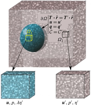
A schematic diagram showing the outline of the problem and the matching boundary condition at the interface between the two domains. Both domains consist of a viscous matrix and an interstitial fluid. The ratio between the shear viscosity of the inner matrix over that of the outer matrix is given by
 $\unicode[STIX]{x1D706}$
. The two boundary conditions indicate continuity of velocity and traction across the interface. Two representative unit volumes within each domain are shown in zooms. Each of these unit volumes consist of a matrix and an interstitial fluid.

2 Theory
2.1 Governing equations
Consider a spherical, multiphase domain embedded in a multiphase substrate. Both of these domains consist of two interconnected phases: a load-bearing, viscous matrix and an inviscid interstitial fluid. We designate the sphere as the inner domain (
 $\unicode[STIX]{x1D6FA}_{1}$
) and the substrate as the outer domain (
 $\unicode[STIX]{x1D6FA}_{2}$
), separated by an interface
 $\unicode[STIX]{x2202}\unicode[STIX]{x1D6FA}$
. The schematic diagram in figure 1 outlines the domains, the boundaries, the key variables and boundary conditions. We apply a known, external velocity to the substrate, which induces creeping motion of the matrix within both domains. Within each domain, flow of the matrix leads to matrix compaction and segregation of the interstitial fluid. Matrix flow, normal forces, flux of interstitial fluid and compaction between the two domains, the sphere and the substrate, are controlled by a set of boundary conditions at the interface between the sphere and the substrate. We use primed variables for the substrate and unprimed variables for the sphere. During the derivation of the governing equations, however, we use unprimed variables, and note that these generalized equations apply for both domains. We use boldface serif font to denote vectors and boldface sans serif fonts to denote tensors. Finally, we note that the ratio of the shear viscosity of the matrix of the sphere and the matrix of the substrate is given by the dimensionless variable
 $\unicode[STIX]{x1D706}$
.
Within each domain, the volume fraction of the interstitial fluid is given by the variable
 $\unicode[STIX]{x1D719}$
. While the densities of all the phases are constant, compaction of the two-phase aggregate can lead to change in the total volume of the matrix and interstitial fluid in a unit volume. As a result, the aggregates in each domain are associated with an effective bulk viscosity (McKenzie Reference McKenzie1984; Bercovici et al.
Reference Bercovici, Ricard and Schubert2001a
; Ricard et al.
Reference Ricard, Bercovici and Schubert2001). Viscous flow of the interstitial fluid through an interconnected network of throats and pores is governed by Darcy flow (McKenzie Reference McKenzie1984). Relative motion between the two phases leads to frictional resistance at the interface between the fluid and the matrix (Bercovici et al.
Reference Bercovici, Ricard and Schubert2001a
; Hier-Majumder Reference Hier-Majumder2011). The constitutive equations for the effective physical properties, such as the bulk viscosity and frictional resistance, arise from the microstructural models implicitly assumed. While a detailed description of the microstructural models is beyond the scope of this article, the interested reader can find more detailed descriptions in a number of published articles (Bercovici et al.
Reference Bercovici, Ricard and Schubert2001a
; Hier-Majumder Reference Hier-Majumder2008; Takei & Hier-Majumder Reference Takei and Hier-Majumder2009; Hier-Majumder & Abbott Reference Hier-Majumder and Abbott2010; Simpson et al.
Reference Simpson, Spiegelman and Weinstein2010a
; King, Hier-Majumder & Kohlstedt Reference King, Hier-Majumder and Kohlstedt2011; Wimert & Hier-Majumder Reference Wimert and Hier-Majumder2012; Drombosky & Hier-Majumder Reference Drombosky and Hier-Majumder2015; Hier-Majumder & Drombosky Reference Hier-Majumder and Drombosky2015).
The complete set of governing equations within each domain consists of a mass and momentum conservation equation for each phase supplemented by a set of constitutive equations arising from the conservation of entropy and Onsager’s principle. For the sake of brevity, the reader is referred to these references for a detailed derivation of the governing equations. Here we present a short derivation of the equations in terms of matrix velocity and reduced fluid pressure in appendix A.
In the absence of melting or freezing, the equation for conservation of mass of the matrix can be expressed in terms of the material time derivative of the interstitial fluid volume fraction as
 $$\begin{eqnarray}\frac{\text{D}\unicode[STIX]{x1D719}}{\text{D}t}=\frac{\unicode[STIX]{x2202}\unicode[STIX]{x1D719}}{\unicode[STIX]{x2202}t}+\boldsymbol{u}\boldsymbol{\cdot }\unicode[STIX]{x1D735}\unicode[STIX]{x1D719}=(1-\unicode[STIX]{x1D719})\unicode[STIX]{x1D735}\boldsymbol{\cdot }\boldsymbol{u},\end{eqnarray}$$
where
 $\boldsymbol{u}$
is the velocity and
 $1-\unicode[STIX]{x1D719}$
is the volume fraction of the matrix. The material time derivative of the fluid volume fraction on the left-hand side of (2.1) represents the rate of fluid loss or gain from a unit volume of the multiphase aggregate. The unit volumes within each domain are shown in the schematic diagram in figure 1. Since the fluid volume fraction depends on time and space, this derivative is non-zero, rendering the matrix velocity divergent. Later in the solution building process, we define the divergence of the matrix velocity as compaction.
The mass conservation equation is supplemented by two coupled partial differential equations (PDEs) for momentum conservation as outlined in appendix A. This leads to the following two PDEs in
 $\boldsymbol{u}$
and the reduced pressure
 $p$
, within each domain
 $\unicode[STIX]{x1D6FA}_{i}$
(
 $i=1,2$
),
 $$\begin{eqnarray}\displaystyle & \unicode[STIX]{x1D735}[\unicode[STIX]{x1D6FC}_{\unicode[STIX]{x1D719}}\unicode[STIX]{x1D735}\boldsymbol{\cdot }\boldsymbol{u}]+\unicode[STIX]{x1D735}\boldsymbol{\cdot }[\unicode[STIX]{x1D702}_{\unicode[STIX]{x1D719}}\unicode[STIX]{x1D73A}(\boldsymbol{u})]-\unicode[STIX]{x1D735}p=0, & \displaystyle\end{eqnarray}$$
 $$\begin{eqnarray}\displaystyle & \unicode[STIX]{x1D735}\boldsymbol{\cdot }[\boldsymbol{u}-\unicode[STIX]{x1D719}^{2}\unicode[STIX]{x1D648}_{0}\boldsymbol{\cdot }\unicode[STIX]{x1D735}p]=0, & \displaystyle\end{eqnarray}$$
where
 $\unicode[STIX]{x1D648}_{0}=\unicode[STIX]{x1D63E}^{-1}$
is the mobility tensor (Hier-Majumder Reference Hier-Majumder2011). The mobility tensor is associated with the more commonly used permeability tensor in porous flow models. The functions
 $\unicode[STIX]{x1D6FC}_{\unicode[STIX]{x1D719}}$
and
 $\unicode[STIX]{x1D702}_{\unicode[STIX]{x1D719}}$
are given by
 $$\begin{eqnarray}\displaystyle & \displaystyle \unicode[STIX]{x1D6FC}_{\unicode[STIX]{x1D719}}=\frac{2\unicode[STIX]{x1D702}(1-\unicode[STIX]{x1D719})(2-\unicode[STIX]{x1D719})}{3\unicode[STIX]{x1D719}}=\unicode[STIX]{x1D6FD}\unicode[STIX]{x1D702}_{\unicode[STIX]{x1D719}}, & \displaystyle\end{eqnarray}$$
 $$\begin{eqnarray}\displaystyle & \displaystyle \unicode[STIX]{x1D702}_{\unicode[STIX]{x1D719}}=\unicode[STIX]{x1D702}(1-\unicode[STIX]{x1D719}), & \displaystyle\end{eqnarray}$$
where
 $\unicode[STIX]{x1D6FD}$
is a function of
 $\unicode[STIX]{x1D719}$
. Similar to the formulations of Alisic et al. (Reference Alisic, Rudge, Katz, Wells and Rhebergen2014) and Rhebergen et al. (Reference Rhebergen, Wells, Katz and Wathen2014, Reference Rhebergen, Wells, Wathen and Katz2015),
 $\unicode[STIX]{x1D6FC}_{\unicode[STIX]{x1D719}}$
represents an effective bulk viscosity within each domain. Note that this expression of
 $\unicode[STIX]{x1D6FC}_{\unicode[STIX]{x1D719}}$
becomes singular in the limit
 $\unicode[STIX]{x1D719}\rightarrow 0$
. The effective bulk viscosity of a unit volume in a multiphase aggregate depends on certain assumptions about the distribution and geometry of the phases in the unit volume (Bercovici et al.
Reference Bercovici, Ricard and Schubert2001a
; Simpson et al.
Reference Simpson, Spiegelman and Weinstein2010a
). As
 $\unicode[STIX]{x1D719}\rightarrow 0$
, these underlying assumptions become invalid and the effective bulk viscosity becomes unbounded. Despite the presence of this singularity, we note that this term becomes large as the interstitial fluid volume fraction decreases, indicating that it requires more work to compact a relatively dry unit volume.
In both domains, the matrix acts as the load-bearing unit (Bercovici et al.
Reference Bercovici, Ricard and Schubert2001a
). As a result, the average normal traction across the sphere–substrate interface will be borne by the matrix on each domain. To evaluate this, we start with the definition of the stress tensor in the matrix,
 $\unicode[STIX]{x1D64F}$
, using the constitutive relation
 $$\begin{eqnarray}\unicode[STIX]{x1D64F}=[\unicode[STIX]{x1D6FC}\unicode[STIX]{x1D735}\boldsymbol{\cdot }\boldsymbol{u}-p]\unicode[STIX]{x1D644}+\unicode[STIX]{x1D702}\unicode[STIX]{x1D73A}(\boldsymbol{u}),\quad \text{in }\unicode[STIX]{x1D6FA}_{i}\;(i=1,2),\end{eqnarray}$$
where
 $\unicode[STIX]{x1D6FC}=\unicode[STIX]{x1D6FC}_{\unicode[STIX]{x1D719}}/(1-\unicode[STIX]{x1D719})$
. For small values of
 $\unicode[STIX]{x1D719}$
(
 $\unicode[STIX]{x1D719}\ll 1$
),
 $\unicode[STIX]{x1D702}=\unicode[STIX]{x1D702}_{\unicode[STIX]{x1D719}}$
and
 $\unicode[STIX]{x1D6FC}=\unicode[STIX]{x1D6FC}_{\unicode[STIX]{x1D719}}$
. For the sake of simplicity, we build solutions in this limit through the rest of this paper and use the symbol
 $\unicode[STIX]{x1D6FC}$
to denote the effective bulk viscosity. We define the parameter
 $\unicode[STIX]{x1D6FD}=\unicode[STIX]{x1D6FC}/\unicode[STIX]{x1D702}$
, the ratio between the bulk and shear viscosities. We also assume that the role of gravity is negligible, such that the fluid pressure can be replaced by the reduced pressure.
2.2 Non-dimensionalization
We non-dimensionalize the lengths with a characteristic length scale
 $L$
, and using a characteristic velocity of magnitude
 $u_{0}$
, we non-dimensionalize the velocity, stress and pressure. Finally, we use a reference value of interstitial friction,
 $c$
(Hier-Majumder Reference Hier-Majumder2011), to non-dimensionalize the mobility. This leads to the following non-dimensionalized variables marked by an asterisk (
 $^{\ast }$
):
 $$\begin{eqnarray}\displaystyle & \displaystyle \boldsymbol{u}=u_{0}\boldsymbol{u}^{\ast }, & \displaystyle\end{eqnarray}$$
 $$\begin{eqnarray}\displaystyle & \displaystyle \unicode[STIX]{x1D64F},p={\displaystyle \frac{\unicode[STIX]{x1D702}u_{0}}{L}}(\unicode[STIX]{x1D64F}^{\ast },p^{\ast }) & \displaystyle\end{eqnarray}$$
and
 $$\begin{eqnarray}\unicode[STIX]{x1D648}_{0}=\frac{1}{c}\unicode[STIX]{x1D648}^{\ast }.\end{eqnarray}$$
Through the rest of the article, we drop the asterisk from the dimensionless variables, unless noted otherwise. In this notation, the non-dimensional versions of the two momentum conservation equations (2.2) and (2.3) become
 $$\begin{eqnarray}\displaystyle & \displaystyle \unicode[STIX]{x1D735}[\unicode[STIX]{x1D6FC}\unicode[STIX]{x1D735}\boldsymbol{\cdot }\boldsymbol{u}]+\unicode[STIX]{x1D735}\boldsymbol{\cdot }[\unicode[STIX]{x1D702}\unicode[STIX]{x1D73A}(\boldsymbol{u})]-\unicode[STIX]{x1D735}p=0, & \displaystyle\end{eqnarray}$$
 $$\begin{eqnarray}\displaystyle & \displaystyle \unicode[STIX]{x1D735}\boldsymbol{\cdot }\left[\boldsymbol{u}-\left(\frac{\unicode[STIX]{x1D6FF}}{L}\right)^{2}\unicode[STIX]{x1D648}\boldsymbol{\cdot }\unicode[STIX]{x1D735}p\right]=0, & \displaystyle\end{eqnarray}$$
where
 $\unicode[STIX]{x1D6FF}=\sqrt{\unicode[STIX]{x1D702}/c}$
is called the compaction length of the matrix (McKenzie Reference McKenzie1984; Bercovici et al.
Reference Bercovici, Ricard and Schubert2001a
). It is a characteristic length scale over which pore fluid can significantly segregate from the matrix.
To build analytical solutions, we make a few more simplifying assumptions. First, we treat
 $\unicode[STIX]{x1D6FC}$
and
 $\unicode[STIX]{x1D702}$
as constants. While both of these terms are dependent on
 $\unicode[STIX]{x1D719}$
, which can vary spatially and temporally, this assumption decouples such variations from our solutions (Rudge Reference Rudge2014). Spiegelman (Reference Spiegelman1993a
,Reference Spiegelman
b
) also discusses the issues associated with this assumption. The analytical solutions presented here are valid only for very short periods of time following the onset of the flow, as the coupling between the terms discussed above becomes crucial for later stages of the flow. Next, we assume that the mobility of the fluid,
 $c\unicode[STIX]{x1D648}_{0}=\unicode[STIX]{x1D644}$
, rendering
 $\unicode[STIX]{x1D648}^{\ast }=\unicode[STIX]{x1D644}$
and constraining
 $c$
in terms of matrix viscosity. Finally, we assume that the compaction length,
 $\unicode[STIX]{x1D6FF}$
, is equal to the characteristic length scale,
 $L$
, of the matrix, and both are equal to the dimensional radius of the sphere. Rudge (Reference Rudge2014) presents results for varying compaction length on the outer flow.
We can further simplify the governing PDE (2.10) by noting the identity
 $$\begin{eqnarray}\unicode[STIX]{x1D735}\boldsymbol{\cdot }\unicode[STIX]{x1D73A}(\boldsymbol{u})=2\unicode[STIX]{x1D735}(\unicode[STIX]{x1D735}\boldsymbol{\cdot }\boldsymbol{u})-\unicode[STIX]{x1D735}\times \unicode[STIX]{x1D735}\times \boldsymbol{u},\end{eqnarray}$$
which, in addition to the assumptions discussed earlier, leads to the simplified PDEs in each domain
 $\unicode[STIX]{x1D6FA}_{i}~(i=1,2)$
:
 $$\begin{eqnarray}\displaystyle & \displaystyle \unicode[STIX]{x1D735}(\unicode[STIX]{x1D735}\boldsymbol{\cdot }\boldsymbol{u})-\frac{1}{\unicode[STIX]{x1D6FC}+2\unicode[STIX]{x1D702}}\unicode[STIX]{x1D735}p-\frac{\unicode[STIX]{x1D702}}{\unicode[STIX]{x1D6FC}+2\unicode[STIX]{x1D702}}\unicode[STIX]{x1D735}\times \unicode[STIX]{x1D735}\times \boldsymbol{u}=0, & \displaystyle\end{eqnarray}$$
 $$\begin{eqnarray}\displaystyle & \displaystyle \unicode[STIX]{x1D735}\boldsymbol{\cdot }\boldsymbol{u}-\unicode[STIX]{x1D6FB}^{2}p=0. & \displaystyle\end{eqnarray}$$
We note that these equations are similar in nature to those in Spiegelman (Reference Spiegelman1993a ). Next, we proceed to construct analytical solutions for the potential functions. Owing to the linear nature of the governing equations, general solutions for the potentials, containing unknown constant coefficients, can be superposed to obtain general solutions for velocity and pressure. The values of these unknown coefficients are then obtained by matching the boundary conditions. I present the results for two types of problems based on two types of boundary conditions. These boundary conditions are discussed in § 2.3.
2.3 Boundary conditions and solution for the coefficients
This section presents solutions for the unknown constants in the formulation for velocity and pressure in the sphere and the surrounding substrate. The values of these unknown constants are determined from the boundary conditions. The boundary conditions themselves depend on the nature of the problem to be investigated. Here, two primary types of problems are identified. The first class of problems concern the solutions internal only to the sphere. This group of solutions complements the solutions for the substrate only, as discussed by Rudge (Reference Rudge2014). The second set of problems arise from coupling of the flow within the sphere and substrate. This set of problems is particularly interesting for studying the distribution of interstitial melt within the deformable sphere. While our approximation of constant
 $\unicode[STIX]{x1D6FC}$
,
 $\unicode[STIX]{x1D702}$
and permeability restricts the validity of these solutions only during the onset of flow, they still provide useful insight into the nature of the flows.
For the first class of problems, the substrate is considered effectively rigid. As a result, the sphere remains undeformed during the flow. Under these conditions, the restrictions on the continuity of traction can be relaxed. A more interesting boundary condition for this problem is imposing a Neumann condition on pressure. As a general case, we can express these boundary conditions as
 $$\begin{eqnarray}\displaystyle \left.\begin{array}{@{}c@{}}\boldsymbol{u}=\boldsymbol{u}_{s},\\ \unicode[STIX]{x1D735}p\boldsymbol{\cdot }\hat{\boldsymbol{n}}=q_{s},\end{array}\right\}\quad \text{on }\unicode[STIX]{x2202}\unicode[STIX]{x1D6FA}, & & \displaystyle\end{eqnarray}$$
where
 $\boldsymbol{u}_{s}$
is a prescribed matrix velocity at the surface and
 $q_{s}$
is a prescribed interstitial fluid flux at the surface of the sphere. Inserting the definition of modified pressure from (A 9) into the Darcy equation, and non-dimensionalizing, we obtain
 $$\begin{eqnarray}\unicode[STIX]{x0394}\boldsymbol{u}=\unicode[STIX]{x1D719}\unicode[STIX]{x1D735}p.\end{eqnarray}$$
The second boundary condition on the normal gradient of pressure, therefore, allows the prescription of the flux of the interstitial fluid into or out of the sphere. Such a prescription is desirable for problems involving an impermeable boundary or problems of passive (since no reaction is involved) interstitial fluid injection. Problems involving flooding of hydrocarbon reservoirs during secondary recovery fall in this category (Gunde, Bera & Mitra Reference Gunde, Bera and Mitra2010). While this boundary condition prescribes the normal flow of interstitial fluid given by
 $\unicode[STIX]{x0394}\boldsymbol{u}\boldsymbol{\cdot }\hat{\boldsymbol{n}}$
, no restrictions are imposed on the tangential component of the segregation velocity. This component adjusts itself based on the solution for pressure.
The second class of problems constitutes coupling of flow between the sphere and the substrate, involving deformation of the boundary between the two domains. A number of previous studies on similar problems for spherical, single-phase drops embedded in a single-phase substrate outline two criteria for the boundary condition (Taylor Reference Taylor1932; Pozrikidis Reference Pozrikidis1990; Hopper Reference Hopper1993a ,Reference Hopper b ; Kuiken Reference Kuiken1993; Li et al. Reference Li, Zhou and Pozrikidis1995; Manga & Stone Reference Manga and Stone1995; Li & Pozrikidis Reference Li and Pozrikidis1996; Loewenberg & Hinch Reference Loewenberg and Hinch1996; Manga et al. Reference Manga, Castro, Cashman and Loewenberg1998; Manga & Loewenberg Reference Manga and Loewenberg2001; Rust & Manga Reference Rust and Manga2002; Hier-Majumder Reference Hier-Majumder2008, Reference Hier-Majumder2011; Hier-Majumder & Abbott Reference Hier-Majumder and Abbott2010).
The first criterion requires that the velocity within the two domains must be matched at the boundary. For example, if the surface of the sphere (the interface
 $\unicode[STIX]{x2202}\unicode[STIX]{x1D6FA}$
) is defined by a shape function
 $F=0$
, then, assuming that the matrix is the load-bearing phase, the kinetic equation governing the shape evolution of the sphere is given by Hier-Majumder (Reference Hier-Majumder2008, equation (11))
 $$\begin{eqnarray}\frac{\unicode[STIX]{x2202}F}{\unicode[STIX]{x2202}t}+\boldsymbol{u}\boldsymbol{\cdot }\hat{\boldsymbol{n}}=0.\end{eqnarray}$$
Thus, the surface is advected by the normal component of the matrix velocity. If the velocities on both sides of the interface are unmatched, then the advection equation will lead to either protrusion of one domain into the other or creation of empty space between the two domains. For problems involving deformation of the interface, therefore, it is crucial to ensure the continuity of velocity across the interface.
Also, the traction at the boundary between the sphere and the substrate must be matched in order to ensure that the sphere and the substrate exert equal and opposite forces on each other (Kim & Karrila Reference Kim and Karrila2005). This boundary condition is further resolved into two components, one normal to the interface and the other tangential. In order to ensure equal and opposite forces, the normal component of the tractions from each domain must be equal. This is often named the Laplace boundary condition. The jump in the tangential component arising from shear stresses has to be matched by the surface parallel gradient of surface tension force acting on the boundary. This component is called the Marangoni condition. In this analysis, we assume that there is no surface tension on
 $\unicode[STIX]{x2202}\unicode[STIX]{x1D6FA}$
, and thus the Laplace and Marangoni terms associated with surface tension do not appear in this boundary condition (e.g. equation (5-70) in Leal Reference Leal1992).
In addition to the continuity of velocity and normal traction, two other constraints arise from interstitial fluid flux and compaction. First, the solutions must ensure that the flux of interstitial fluid is matched across the interface between the two domains. As discussed above, this constraint can be imposed by matching the normal gradient of pressure across the boundary. Note that this condition is not guaranteed by the continuity of velocity and traction. Finally, we require that compaction within both domains must be matched at the boundary also. As the results demonstrate, these constraints ensure a unique solution for the coupled multiphase, multidomain flow.
With these above constraints, we solve for the coefficients for the coupled flow problem subject to the boundary conditions
 $$\begin{eqnarray}\displaystyle \left.\begin{array}{@{}c@{}}\boldsymbol{u}=\boldsymbol{u}^{\prime },\\ \unicode[STIX]{x1D64F}\boldsymbol{\cdot }\hat{\boldsymbol{n}}=\unicode[STIX]{x1D64F}^{\prime }\boldsymbol{\cdot }\hat{\boldsymbol{n}},\\ \unicode[STIX]{x1D735}p\boldsymbol{\cdot }\hat{\boldsymbol{n}}=\unicode[STIX]{x1D735}p^{\prime }\boldsymbol{\cdot }\hat{\boldsymbol{n}},\\ {\mathcal{C}}={\mathcal{C}}^{\prime },\end{array}\right\}\quad \text{on }\unicode[STIX]{x2202}\unicode[STIX]{x1D6FA}, & & \displaystyle\end{eqnarray}$$
where compaction, given by the variable
 ${\mathcal{C}}$
, is defined in the following section. In the following subsections, we present the solutions for the coefficients for the two types of problems discussed above.
3 Solution building
3.1 Potential functions
We seek to build analytical solutions for velocity and pressure within each domain using potential functions. For similar multidomain problems involving Stokes flow, typically vector harmonics are used to build vector and scalar potentials (Happel & Brenner Reference Happel and Brenner1983; Leal Reference Leal1992; Kim & Karrila Reference Kim and Karrila2005). During two-phase flow, an additional potential is needed to account for the divergence of matrix velocity or compaction,
 ${\mathcal{C}}$
, given by (Spiegelman Reference Spiegelman1993a
)
 $$\begin{eqnarray}{\mathcal{C}}=\unicode[STIX]{x1D735}\boldsymbol{\cdot }\boldsymbol{u}.\end{eqnarray}$$
In a recent article, Rudge (Reference Rudge2014) builds analytical solutions for flow in the substrate using Neuber–Papkovitch potentials. In this method, one vector potential
 $\unicode[STIX]{x1D753}$
and two scalar potentials,
 ${\mathcal{C}}$
and
 $\unicode[STIX]{x1D712}$
, are used to build the solutions. In order for the solutions to be independent of coordinate system, these functions are built from the position vector
 $\boldsymbol{r}$
. The matrix velocity and the reduced pressure within each domain can be expressed as a function of these potentials as
 $$\begin{eqnarray}\displaystyle & \boldsymbol{u}=\unicode[STIX]{x1D735}[\boldsymbol{r}\boldsymbol{\cdot }\unicode[STIX]{x1D753}+\unicode[STIX]{x1D712}+{\mathcal{C}}]-2\unicode[STIX]{x1D753}, & \displaystyle\end{eqnarray}$$
 $$\begin{eqnarray}\displaystyle & p=2\unicode[STIX]{x1D702}\unicode[STIX]{x1D735}\boldsymbol{\cdot }\unicode[STIX]{x1D753}+(\unicode[STIX]{x1D6FC}+2\unicode[STIX]{x1D702}){\mathcal{C}}. & \displaystyle\end{eqnarray}$$
Substituting the potential forms of velocity and pressure from (3.2) and (3.3) into (2.13) and (2.14), we obtain three simpler PDEs:
 $$\begin{eqnarray}\displaystyle \unicode[STIX]{x1D6FB}^{2}\unicode[STIX]{x1D753} & = & \displaystyle 0,\end{eqnarray}$$
 $$\begin{eqnarray}\displaystyle \unicode[STIX]{x1D6FB}^{2}\unicode[STIX]{x1D712} & = & \displaystyle 0,\end{eqnarray}$$
 $$\begin{eqnarray}\displaystyle \unicode[STIX]{x1D6FB}^{2}{\mathcal{C}}-{\mathcal{C}} & = & \displaystyle 0.\end{eqnarray}$$
The definition of compaction,
 ${\mathcal{C}}$
in (3.1), combined with the equation for mass conservation (2.1) yields
 $$\begin{eqnarray}\frac{\text{D}\unicode[STIX]{x1D719}}{\text{D}t}=(1-\unicode[STIX]{x1D719}){\mathcal{C}}.\end{eqnarray}$$
For very small fluid fractions,
 $\unicode[STIX]{x1D719}\ll 1$
and
 $\text{D}\unicode[STIX]{x1D719}/\text{D}t\approx {\mathcal{C}}$
. This implies that, in the early stages of compaction containing a small volume fraction of pore fluid, the fluid will accumulate (
 $\text{D}\unicode[STIX]{x1D719}/\text{D}t>0$
) in regions of positive compaction (dilatation) and drain out of regions of negative compaction. While this is a zeroth-order approximation, this relation provides us with an insight about the nature of phase segregation within each domain as a result of the coupled flow.
A general far-field flow in the substrate can consist of a straining component, a rotating component and a translating component (Leal Reference Leal1992, chap. 4). For solutions arising from a purely straining flow, the rotating and translating components of the far-field flow can be neglected. As we focus on the flow field due to a purely straining flow, we will use this strategy for building the solution. The straining component is built from the symmetric strain-rate tensor
 $\dot{\unicode[STIX]{x1D640}}$
, such that
 $\text{Tr}(\dot{\unicode[STIX]{x1D640}})=0$
. The primary variables, velocity and pressure, are built from the characteristic scalar
 $\dot{\unicode[STIX]{x1D640}}\mathbf{: }\boldsymbol{r}\boldsymbol{r}$
, and two characteristic vectors,
 $\dot{\unicode[STIX]{x1D640}}\boldsymbol{\cdot }\boldsymbol{r}$
and
 $(\dot{\unicode[STIX]{x1D640}}\mathbf{: }\boldsymbol{r}\boldsymbol{r})\boldsymbol{r}$
, respectively.
While the influence of far-field flow is incorporated in the solution by the methods discussed above, the remaining part of the solution is built from fundamental solutions to the Laplace and the modified Helmholtz equations. An important consideration in building solutions is the behaviour of the solution at the origin
 $r=0$
and at large distances away from the sphere,
 $r\rightarrow \infty$
. We discuss these issues in the next subsection.
At this stage, it is useful to define a few additional relations for derived variables in terms of these potential functions:
 $$\begin{eqnarray}\displaystyle & \displaystyle \dot{\unicode[STIX]{x1D65A}}={\textstyle \frac{1}{2}}\unicode[STIX]{x1D73A}(\boldsymbol{u})=(\unicode[STIX]{x1D735}\unicode[STIX]{x1D735}\unicode[STIX]{x1D753})\boldsymbol{\cdot }\boldsymbol{r}+\unicode[STIX]{x1D735}\unicode[STIX]{x1D735}(\unicode[STIX]{x1D712}+{\mathcal{C}}), & \displaystyle\end{eqnarray}$$
 $$\begin{eqnarray}\displaystyle & \displaystyle P_{m}=2\unicode[STIX]{x1D702}\unicode[STIX]{x1D735}\boldsymbol{\cdot }\unicode[STIX]{x1D753}+(\unicode[STIX]{x1D6FC}+\bar{\unicode[STIX]{x1D702}}){\mathcal{C}}, & \displaystyle\end{eqnarray}$$
 $$\begin{eqnarray}\displaystyle & \displaystyle \unicode[STIX]{x1D64F}=2\unicode[STIX]{x1D702}[-(\unicode[STIX]{x1D735}\boldsymbol{\cdot }\unicode[STIX]{x1D753}+{\mathcal{C}})+{\textstyle \frac{1}{2}}\unicode[STIX]{x1D73A}(\boldsymbol{u})], & \displaystyle\end{eqnarray}$$
 $$\begin{eqnarray}\displaystyle & \displaystyle \boldsymbol{t}=\unicode[STIX]{x1D64F}\boldsymbol{\cdot }\hat{\boldsymbol{n}}=\frac{2\unicode[STIX]{x1D702}}{r}[-(\unicode[STIX]{x1D735}\boldsymbol{\cdot }\unicode[STIX]{x1D753})\boldsymbol{r}-{\mathcal{C}}\boldsymbol{r}+{\textstyle \frac{1}{2}}\unicode[STIX]{x1D73A}(\boldsymbol{u})\boldsymbol{\cdot }\boldsymbol{r}], & \displaystyle\end{eqnarray}$$
where
 $\bar{\unicode[STIX]{x1D702}}=2\unicode[STIX]{x1D702}(3\unicode[STIX]{x1D719}-2)/(3\unicode[STIX]{x1D719})$
.
In the following subsections, we discuss the selection of functions involved in the solution building.
3.2 Growing and decaying functions
We build solutions for the potential functions
 $\unicode[STIX]{x1D753}$
and
 $\unicode[STIX]{x1D712}$
from vector harmonic functions (Leal Reference Leal1992). Vector harmonics are derived from the fundamental solution to the Laplace equation, which satisfies the inhomogeneous equation
 $$\begin{eqnarray}-\unicode[STIX]{x1D6FB}^{2}\unicode[STIX]{x1D712}=\unicode[STIX]{x1D6FF}^{(3)}(\boldsymbol{r}),\end{eqnarray}$$
where
 $\unicode[STIX]{x1D6FF}^{3}(\boldsymbol{r})$
is the three-dimensional Dirac delta function centred around a point located at position
 $\boldsymbol{r}$
. One family of solutions, decaying harmonics, are built from the fundamental solution and its successive derivatives (Leal Reference Leal1992, chap. 4).
While the vector harmonic functions are useful for building solutions for the vector and scalar Laplace equations, the presence of the modified Helmholtz equation calls for an additional fundamental solution. We note that the fundamental solution to the modified Helmholtz equation should satisfy the equation
 $$\begin{eqnarray}-{\mathcal{C}}+\unicode[STIX]{x1D6FB}^{2}{\mathcal{C}}=\unicode[STIX]{x1D6FF}^{(3)}(\boldsymbol{r}).\end{eqnarray}$$
Following a similar reason as above, the solutions to the modified Helmholtz equation arising from the internal and the external flow can be built from the fundamental solution and its derivatives decaying as
 $r\rightarrow 0$
and
 $r\rightarrow \infty$
, respectively. For the internal flow, we build solutions based on the modified spherical Bessel functions of the first kind (Arfken & Weber Reference Arfken and Weber1995, p. 689).
The modified Bessel functions of the first kind decay with
 $r$
and are bound to finite values as
 $r\rightarrow 0$
. A useful recurrence relation involving these functions is
 $$\begin{eqnarray}\unicode[STIX]{x1D735}\left(\frac{i_{n}(r)}{r^{n}}\right)=\frac{i_{n+1}(r)}{r^{n+1}}\boldsymbol{r}.\end{eqnarray}$$
As discussed by Rudge (Reference Rudge2014), the solution for compaction in the substrate can be built from the modified spherical Bessel functions of the second kind. Another useful identity involving these functions is
 $$\begin{eqnarray}\unicode[STIX]{x1D735}\left(\frac{k_{n}(r)}{r^{n}}\right)=-\frac{k_{n+1}(r)}{r^{n+1}}\boldsymbol{r}.\end{eqnarray}$$
3.3 Solutions for internal flow
In this article, we set the origin at the centre of the sphere. Consequently, the solutions for the interior of the sphere need to be built from growing harmonics, preventing singular solutions at the origin. As
 $r$
is always bound by a finite value, the solution is guaranteed to be bound by finite values on both ends. Since the potential functions contain one vector and two scalar potentials, we build the solution by combining lower-order growing vector harmonic functions and the spherical Bessel functions of the first kind with the characteristic scalar
 $\dot{\unicode[STIX]{x1D640}}\mathbf{: }\boldsymbol{r}\boldsymbol{r}$
, and two characteristic vectors
 $\dot{\unicode[STIX]{x1D640}}\boldsymbol{\cdot }\boldsymbol{r}$
and
 $(\dot{\unicode[STIX]{x1D640}}\mathbf{: }\boldsymbol{r}\boldsymbol{r})\boldsymbol{r}$
.
The resulting solutions call for the introduction of three unknown coefficients,
 $F$
,
 $G$
and
 $H$
, leading to the following definitions of the potential functions:
 $$\begin{eqnarray}\displaystyle & \displaystyle \unicode[STIX]{x1D753}=\frac{2F}{5}(1-r^{2})\dot{\unicode[STIX]{x1D640}}\boldsymbol{\cdot }\boldsymbol{r}+\boldsymbol{r}(\dot{\unicode[STIX]{x1D640}}\mathbf{: }\boldsymbol{r}\boldsymbol{r}), & \displaystyle\end{eqnarray}$$
 $$\begin{eqnarray}\displaystyle & \displaystyle \unicode[STIX]{x1D712}=G(\dot{\unicode[STIX]{x1D640}}\mathbf{: }\boldsymbol{r}\boldsymbol{r}), & \displaystyle\end{eqnarray}$$
 $$\begin{eqnarray}\displaystyle & \displaystyle {\mathcal{C}}=\frac{H}{r^{2}}i_{2}(r)(\dot{\unicode[STIX]{x1D640}}\mathbf{: }\boldsymbol{r}\boldsymbol{r}). & \displaystyle\end{eqnarray}$$
Using these definitions, the expressions for velocity, reduced pressure, normal traction and the normal component of pressure gradient are given by
 $$\begin{eqnarray}\displaystyle & \displaystyle \boldsymbol{u}=2\left[Fr^{2}+G+H\frac{i_{2}(r)}{r}\right]\dot{\unicode[STIX]{x1D640}}\boldsymbol{\cdot }\boldsymbol{r}+\left[H\frac{i_{3}(r)}{r^{3}}-\frac{4F}{5}\right](\dot{\unicode[STIX]{x1D640}}\mathbf{: }\boldsymbol{r}\boldsymbol{r})\boldsymbol{r}, & \displaystyle\end{eqnarray}$$
 $$\begin{eqnarray}\displaystyle & \displaystyle p=\left[\frac{42F\unicode[STIX]{x1D702}}{5}+H\left(\unicode[STIX]{x1D6FC}+2\unicode[STIX]{x1D702}\right)\frac{i_{2}(r)}{r^{2}}\right](\dot{\unicode[STIX]{x1D640}}\mathbf{: }\boldsymbol{r}\boldsymbol{r}), & \displaystyle\end{eqnarray}$$
 $$\begin{eqnarray}\displaystyle & \displaystyle \unicode[STIX]{x1D64F}\boldsymbol{\cdot }\boldsymbol{r}=2\unicode[STIX]{x1D702}\!\left[-\frac{19F}{5}-\frac{4Hi_{3}(r)}{r^{3}}\right]\!(\dot{\unicode[STIX]{x1D640}}\mathbf{: }\boldsymbol{r}\boldsymbol{r})\boldsymbol{r}+2\unicode[STIX]{x1D702}\!\left[\frac{16Fr^{2}}{5}+2G+2H\!\left(\frac{i_{3}(r)}{r}+\frac{i_{2}(r)}{r^{2}}\right)\!\right]\!\dot{\unicode[STIX]{x1D640}}\boldsymbol{\cdot }\boldsymbol{r}, & \displaystyle \nonumber\\ \displaystyle & & \displaystyle\end{eqnarray}$$
 $$\begin{eqnarray}\displaystyle & \displaystyle \unicode[STIX]{x1D735}p\boldsymbol{\cdot }\boldsymbol{r}=\left[\frac{84F\unicode[STIX]{x1D702}}{5}+H(\unicode[STIX]{x1D6FC}+2\unicode[STIX]{x1D702})\left(\frac{2i_{2}(r)}{r^{2}}+\frac{i_{3}(r)}{r}\right)\right](\dot{\unicode[STIX]{x1D640}}\mathbf{: }\boldsymbol{r}\boldsymbol{r}). & \displaystyle\end{eqnarray}$$
In addition to these variables, we are also interested in calculating the tensor
 $\dot{\unicode[STIX]{x1D65A}}$
. We find that an additional quantity,
 $\boldsymbol{{\mathcal{E}}}$
, is introduced:
 $$\begin{eqnarray}\displaystyle \dot{\unicode[STIX]{x1D65A}} & = & \displaystyle \left[\frac{6F}{5}+2H\frac{i_{3}(r)}{r^{3}}\right]\boldsymbol{{\mathcal{E}}}+\left[2Fr^{2}+2G+2H\frac{i_{2}(r)}{r^{2}}\right]\dot{\unicode[STIX]{x1D640}}\nonumber\\ \displaystyle & & \displaystyle +\left[-\frac{4F}{5}+H\frac{i_{3}(r)}{r^{3}}\right](\dot{\unicode[STIX]{x1D640}}\mathbf{: }\boldsymbol{r}\boldsymbol{r})\unicode[STIX]{x1D644}+\left[H\frac{i_{4}(r)}{r^{4}}\right](\dot{\unicode[STIX]{x1D640}}\mathbf{: }\boldsymbol{r}\boldsymbol{r})\boldsymbol{r}\boldsymbol{r},\end{eqnarray}$$
where the symmetric dyadic product
 $\boldsymbol{{\mathcal{E}}}$
is given by
 $$\begin{eqnarray}\boldsymbol{{\mathcal{E}}}=\boldsymbol{r}(\dot{\unicode[STIX]{x1D640}}\boldsymbol{\cdot }\boldsymbol{r})+(\dot{\unicode[STIX]{x1D640}}\boldsymbol{\cdot }\boldsymbol{r})\boldsymbol{r}.\end{eqnarray}$$
Next, we plan to build solutions for external flow, using similar functions of the far-field straining flow but with decaying functions of
 $r$
.
3.4 Solutions for external flow
In building solutions for the external flow, we recognize that the solution should consist of two parts. One part, which we can call a perturbation flow, arises from the interaction between the substrate and the sphere through the boundary conditions imposed at their interface. This perturbing flow should decay away from the sphere. Thus, we express the total velocity,
 $\boldsymbol{u}^{\prime }$
, as a sum of a far-field uniform straining flow
 $\boldsymbol{u}^{\infty }$
and the local, perturbing flow,
 $$\begin{eqnarray}\boldsymbol{u}^{\prime }=\unicode[STIX]{x1D735}[\boldsymbol{r}\boldsymbol{\cdot }\unicode[STIX]{x1D753}^{\prime }+\unicode[STIX]{x1D712}^{\prime }+{\mathcal{C}}^{\prime }]-2\unicode[STIX]{x1D753}^{\prime }+\boldsymbol{u}^{\infty },\end{eqnarray}$$
subject to the constraint that, as
 $r\rightarrow \infty$
,
 $\boldsymbol{u}^{\prime }\rightarrow \boldsymbol{u}^{\infty }$
. Next, we want to prescribe a form for
 $\boldsymbol{u}^{\infty }$
, in terms of a characteristic vector associated with the straining flow. One obvious choice is the simplest vector
 $\dot{\unicode[STIX]{x1D640}}\boldsymbol{\cdot }\boldsymbol{r}$
, leading to
 $\boldsymbol{u}^{\infty }=\dot{\unicode[STIX]{x1D640}}\boldsymbol{\cdot }\boldsymbol{r}$
(Leal Reference Leal1992, chap. 4). Note that, since
 $\text{Tr}(\dot{\unicode[STIX]{x1D640}})=0$
,
 $\unicode[STIX]{x1D735}\boldsymbol{\cdot }\boldsymbol{u}^{\infty }=0$
. Consequently, the far-field strain does not introduce any additional terms associated with compaction.
It is worth noting that, for a more general solution, the external flow can be expressed as a sum of a straining flow, a translating flow and a rotating flow. We ignore the latter two components. Consequently, our results apply for irrotational straining flow only. Specifically, we focus on flow arising from pure shear. To build solutions for a simple shear straining flow, the rotational component needs to be included while building the vector
 $\boldsymbol{u}^{\infty }$
(see chap. 4 of Leal (Reference Leal1992) for further discussion).
Similar to the solutions for internal flow, we build the vector and scalar potential functions from the characteristic vector
 $\dot{\unicode[STIX]{x1D640}}\boldsymbol{\cdot }\boldsymbol{r}$
and the scalar
 $\dot{\unicode[STIX]{x1D640}}\mathbf{: }\boldsymbol{r}\boldsymbol{r}$
, leading to the introduction of three new unknown constants,
 $M,~N$
and
 $L$
, whose values will be determined during the next stage:
 $$\begin{eqnarray}\displaystyle & \displaystyle \unicode[STIX]{x1D753}^{\prime }=-\frac{L}{r^{3}}\dot{\unicode[STIX]{x1D640}}\boldsymbol{\cdot }\boldsymbol{r}, & \displaystyle\end{eqnarray}$$
 $$\begin{eqnarray}\displaystyle & \displaystyle \unicode[STIX]{x1D712}^{\prime }=\frac{3M}{r^{5}}(\dot{\unicode[STIX]{x1D640}}\mathbf{: }\boldsymbol{r}\boldsymbol{r}), & \displaystyle\end{eqnarray}$$
 $$\begin{eqnarray}\displaystyle & \displaystyle {\mathcal{C}}^{\prime }=N\frac{k_{2}(r)}{r^{2}}(\dot{\unicode[STIX]{x1D640}}\mathbf{: }\boldsymbol{r}\boldsymbol{r}). & \displaystyle\end{eqnarray}$$
Since all three of these functions are associated with the coupled flow, they all decay further away from the sphere.
Employing the definitions of the velocity and stresses as above, and utilizing the recurrence relations of the modified spherical Bessel functions, the solutions for velocity, pressure and traction are given by
 $$\begin{eqnarray}\displaystyle & \displaystyle \boldsymbol{u}^{\prime }=\left[\frac{6M}{r^{5}}+2N\frac{k_{2}(r)}{r^{2}}+1\right]\dot{\unicode[STIX]{x1D640}}\boldsymbol{\cdot }\boldsymbol{r}+\left[\frac{3L}{r^{5}}-\frac{15M}{r^{7}}-N\frac{k_{3}(r)}{r^{3}}\right](\dot{\unicode[STIX]{x1D640}}\mathbf{: }\boldsymbol{r}\boldsymbol{r})\boldsymbol{r}, & \displaystyle\end{eqnarray}$$
 $$\begin{eqnarray}\displaystyle & \displaystyle p^{\prime }=\left[\frac{6L\unicode[STIX]{x1D702}^{\prime }}{r^{5}}+(\unicode[STIX]{x1D6FC}^{\prime }+2\unicode[STIX]{x1D702}^{\prime })\frac{Nk_{2}(r)}{r^{2}}\right](\dot{\unicode[STIX]{x1D640}}\mathbf{: }\boldsymbol{r}\boldsymbol{r}), & \displaystyle\end{eqnarray}$$
 $$\begin{eqnarray}\displaystyle \unicode[STIX]{x1D64F}^{\prime }\boldsymbol{\cdot }\boldsymbol{r} & = & \displaystyle 2\unicode[STIX]{x1D702}^{\prime }\left[-\frac{12L}{r^{5}}+\frac{60M}{r^{7}}+\frac{4Nk_{3}(r)}{r^{3}}\right](\dot{\unicode[STIX]{x1D640}}\mathbf{: }\boldsymbol{r}\boldsymbol{r})\boldsymbol{r}\nonumber\\ \displaystyle & & \displaystyle +\,2\unicode[STIX]{x1D702}^{\prime }\left[\frac{3L}{r^{3}}-\frac{24M}{r^{5}}+2N\left(\frac{k_{2}(r)}{r^{2}}-\frac{k_{3}(r)}{r}\right)+1\right]\dot{\unicode[STIX]{x1D640}}\boldsymbol{\cdot }\boldsymbol{r},\end{eqnarray}$$
 $$\begin{eqnarray}\displaystyle \unicode[STIX]{x1D735}p^{\prime }\boldsymbol{\cdot }\boldsymbol{r}=\left[-\frac{18L\unicode[STIX]{x1D702}^{\prime }}{r^{5}}+N(\unicode[STIX]{x1D6FC}^{\prime }+2\unicode[STIX]{x1D702}^{\prime })\left(\frac{2k_{2}(r)}{r^{2}}-\frac{k_{3}(r)}{r}\right)\right](\dot{\unicode[STIX]{x1D640}}\mathbf{: }\boldsymbol{r}\boldsymbol{r}). & & \displaystyle\end{eqnarray}$$
Similar to the internal flow, we see the introduction of the additional symmetric dyad
 $\boldsymbol{{\mathcal{E}}}$
in the definition of the strain-rate field
 $\dot{\unicode[STIX]{x1D65A}}$
:
 $$\begin{eqnarray}\displaystyle \dot{\unicode[STIX]{x1D65A}}^{\prime } & = & \displaystyle \left[-\frac{15L}{r^{7}}+\frac{105M}{r^{9}}+\frac{Nk_{4}(r)}{r^{4}}\right](\dot{\unicode[STIX]{x1D640}}\mathbf{: }\boldsymbol{r}\boldsymbol{r})\boldsymbol{r}\boldsymbol{r}\nonumber\\ \displaystyle & & \displaystyle +\left[\frac{3L}{r^{5}}-\frac{30M}{r^{7}}-\frac{2Nk_{3}(r)}{r^{3}}\right]\boldsymbol{{\mathcal{E}}}+\left[\frac{3L}{r^{5}}-\frac{15M}{r^{7}}-\frac{Nk_{3}(r)}{r^{3}}\right](\dot{\unicode[STIX]{x1D640}}\mathbf{: }\boldsymbol{r}\boldsymbol{r})\unicode[STIX]{x1D644}\nonumber\\ \displaystyle & & \displaystyle +\left[\frac{6M}{r^{5}}+\frac{2Nk_{2}(r)}{r^{2}}+1\right]\dot{\unicode[STIX]{x1D640}}.\end{eqnarray}$$
Similar to the definitions of the velocity and traction vectors for the internal flow, the variables for the external flow are composed of two characteristic vectors,
 $\dot{\unicode[STIX]{x1D640}}\boldsymbol{\cdot }\boldsymbol{r}$
and
 $(\dot{\unicode[STIX]{x1D640}}\mathbf{: }\boldsymbol{r}\boldsymbol{r})\boldsymbol{r}$
. The next step in the solution building involves matching the coefficients of these vectors at the interface using the boundary conditions given in (2.18). Finally, we define the strain-rate tensor
 $\dot{\unicode[STIX]{x1D640}}$
as
 $$\begin{eqnarray}\dot{\unicode[STIX]{x1D640}}=\left[\begin{array}{@{}ccc@{}}{\textstyle \frac{1}{2}} & 0 & 0\\ 0 & {\textstyle \frac{1}{2}} & 0\\ 0 & 0 & -1\end{array}\right].\end{eqnarray}$$
3.5 Coefficients for internal flow
3.5.1 Straining flow
Consider an impermeable sphere subjected to a straining flow. Since the segregation velocity of the interstitial fluid from the matrix is governed by the normal component of the pressure gradient, we can rewrite the boundary conditions in (2.15) as
 $$\begin{eqnarray}\displaystyle \left.\begin{array}{@{}c@{}}\boldsymbol{u}=\dot{\unicode[STIX]{x1D640}}\boldsymbol{\cdot }\boldsymbol{r},\\ \unicode[STIX]{x1D735}p\boldsymbol{\cdot }\hat{\boldsymbol{n}}=0,\end{array}\right\}\quad \text{on }\unicode[STIX]{x2202}\unicode[STIX]{x1D6FA}. & & \displaystyle\end{eqnarray}$$
Using the coefficients of the terms in (3.19) and (3.22), we arrive at the following three algebraic equations:
 $$\begin{eqnarray}\displaystyle & \displaystyle 1=2Fa^{2}+2G+2\frac{Hi_{2}(a)}{a^{2}}, & \displaystyle\end{eqnarray}$$
 $$\begin{eqnarray}\displaystyle & \displaystyle 0=\frac{Hi_{3}(a)}{a^{3}}-\frac{4F}{5}, & \displaystyle\end{eqnarray}$$
 $$\begin{eqnarray}\displaystyle & \displaystyle 0=\frac{84F\unicode[STIX]{x1D702}}{5}+H(\unicode[STIX]{x1D6FC}+2\unicode[STIX]{x1D702})\left(\frac{2i_{2}(a)}{a^{2}}+\frac{i_{3}(a)}{a}\right). & \displaystyle\end{eqnarray}$$
Solution of these equations leads to
 $$\begin{eqnarray}\displaystyle & \displaystyle F=0, & \displaystyle\end{eqnarray}$$
 $$\begin{eqnarray}\displaystyle & \displaystyle G={\textstyle \frac{1}{2}}, & \displaystyle\end{eqnarray}$$
 $$\begin{eqnarray}\displaystyle & \displaystyle H=0. & \displaystyle\end{eqnarray}$$
As a result, the internal velocity mimics the straining flow.
3.5.2 Passive melt injection
A second interesting case involves melt injection into the sphere. To prescribe a spatially varying melt injection leading to a non-trivial solution within the sphere, we chose the following:
 $$\begin{eqnarray}\displaystyle \left.\begin{array}{@{}c@{}}\boldsymbol{u}=0,\\ \unicode[STIX]{x1D735}p\boldsymbol{\cdot }\hat{\boldsymbol{n}}=\dot{\unicode[STIX]{x1D640}}\boldsymbol{ : }\boldsymbol{ r}\boldsymbol{ r},\end{array}\right\}\quad \text{on }\unicode[STIX]{x2202}\unicode[STIX]{x1D6FA}. & & \displaystyle\end{eqnarray}$$
Substituting the solutions for pressure and velocity into these boundary conditions, we arrive at the following three algebraic equations:
 $$\begin{eqnarray}\displaystyle & \displaystyle 0=2Fa^{2}+2G+2\frac{Hi_{2}(a)}{a^{2}}, & \displaystyle\end{eqnarray}$$
 $$\begin{eqnarray}\displaystyle & \displaystyle 0=\frac{Hi_{3}(a)}{a^{3}}-\frac{4F}{5}, & \displaystyle\end{eqnarray}$$
 $$\begin{eqnarray}\displaystyle & \displaystyle 1=\frac{84F\unicode[STIX]{x1D702}}{5}+H(\unicode[STIX]{x1D6FC}+2\unicode[STIX]{x1D702})\left(\frac{2i_{2}(a)}{a^{2}}+\frac{i_{3}(a)}{a}\right). & \displaystyle\end{eqnarray}$$
Solution of these equations lead to the following three values for coefficients,
 $F,~G$
and
 $H$
:
 $$\begin{eqnarray}\displaystyle & \displaystyle F=\frac{5}{4}\frac{i_{3}(a)}{(a^{2}i_{3}(a)+2ai_{2}(a))\unicode[STIX]{x1D6FC}+((2a^{2}+21)i_{3}(a)+4ai_{2}(a))\unicode[STIX]{x1D702}}, & \displaystyle\end{eqnarray}$$
 $$\begin{eqnarray}\displaystyle & \displaystyle G=-\frac{1}{4}\frac{a(5ai_{3}(a)+4i_{2}(a))}{(a^{2}i_{3}(a)+2ai_{2}(a))\unicode[STIX]{x1D6FC}+((2a^{2}+21)i_{3}(a)+4ai_{2}(a))\unicode[STIX]{x1D702}}, & \displaystyle\end{eqnarray}$$
 $$\begin{eqnarray}\displaystyle & \displaystyle H=\frac{5}{4}\frac{i_{3}(a)}{(a^{2}i_{3}(a)+2ai_{2}(a))\unicode[STIX]{x1D6FC}+((2a^{2}+21)i_{3}(a)+4ai_{2}(a))\unicode[STIX]{x1D702}}. & \displaystyle\end{eqnarray}$$
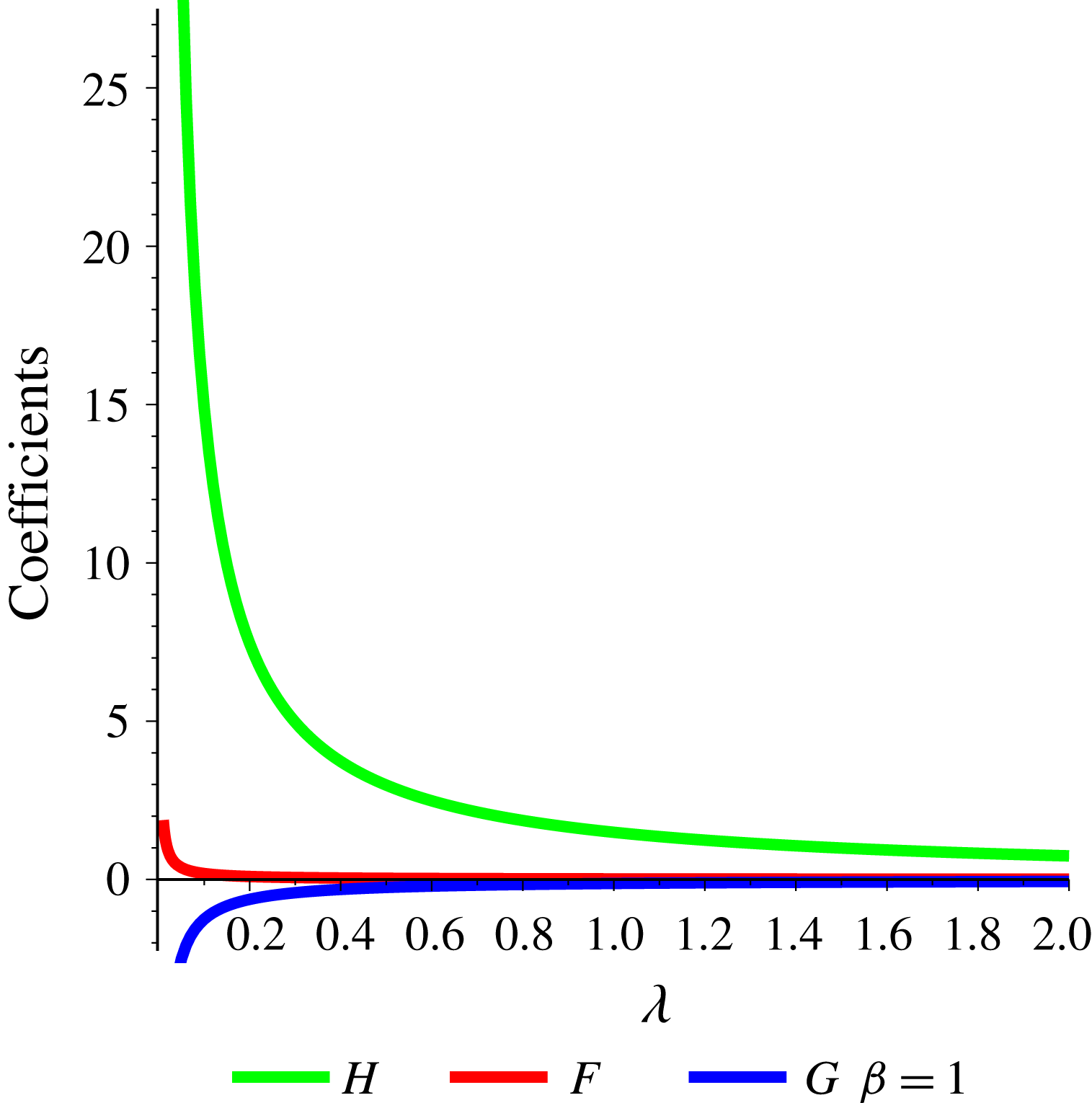
The plots in figure 2 depict the variation in these coefficients, as a function of the matrix viscosity
 $\unicode[STIX]{x1D702}$
, for a value of
 $\unicode[STIX]{x1D6FD}=\unicode[STIX]{x1D6FC}/\unicode[STIX]{x1D702}=1$
and
 $a=1$
. As the plot indicates, the magnitudes of the coefficients decrease, indicating a general reduction in the magnitude of the flow as the matrix becomes more viscous.
A plot of the coefficients
 $F$
,
 $G$
and
 $H$
for internal flow as a function of
 $\unicode[STIX]{x1D702}$
, during the passive melt injection problem. In this plot, we set
 $a=1$
and
 $\unicode[STIX]{x1D6FD}=\unicode[STIX]{x1D6FC}/\unicode[STIX]{x1D702}=1$
.

3.6 Coefficients for coupled flow
We next proceed to match the boundary conditions in (2.18). The solutions contain six unknown constants,
 $F,~G,~H,~M,~N$
and
 $L$
. To solve for these constants, we match the coefficients of the characteristic vectors arising from the far-field flow in the expression for tractions and velocities at the interface between the sphere and the substrate in (2.18), leading to the following four equations:
 $$\begin{eqnarray}\displaystyle & \displaystyle 0=2Fa^{2}+2G+2\frac{Hi_{2}(a)}{a^{2}}-6\frac{M}{a^{5}}-2\frac{Nk_{2}(a)}{a^{2}}-1, & \displaystyle\end{eqnarray}$$
 $$\begin{eqnarray}\displaystyle & \displaystyle 0=\frac{Hi_{3}(a)}{a^{3}}-4/5F-3\frac{L}{a^{5}}+15\frac{M}{a^{7}}+\frac{Nk_{3}(a)}{a^{3}}, & \displaystyle\end{eqnarray}$$
 $$\begin{eqnarray}\displaystyle & \displaystyle 0=\unicode[STIX]{x1D706}\left(-\frac{19F}{5}-4\frac{Hi_{3}(a)}{a^{3}}\right)+12\frac{L}{a^{5}}-60\frac{M}{a^{7}}-4\frac{Nk_{3}(a)}{a^{3}}, & \displaystyle\end{eqnarray}$$
 $$\begin{eqnarray}\displaystyle 0 & = & \displaystyle \unicode[STIX]{x1D706}\left(\frac{16Fa^{2}}{5}+2G+2H\left(\frac{i_{3}(a)}{a}+\frac{i_{2}(a)}{a^{2}}\right)\right)\nonumber\\ \displaystyle & & \displaystyle -\,3\frac{L}{a^{3}}+24\frac{M}{a^{5}}-2N\left(\frac{k_{2}(a)}{a^{2}}-\frac{k_{3}(a)}{a}\right)-1,\end{eqnarray}$$
where
 $\unicode[STIX]{x1D706}=\unicode[STIX]{x1D702}/\unicode[STIX]{x1D702}^{\prime }$
. Note that, since
 $r=a$
on
 $\unicode[STIX]{x2202}\unicode[STIX]{x1D6FA}$
, the equations derived from the boundary conditions are independent of
 $r$
. Also, as the terms in the equations above are coefficients of the characteristic vector and scalars derived from
 $\dot{\unicode[STIX]{x1D640}}$
in (3.19), (3.29), (3.21) and (3.31), they are also independent of
 $\dot{\unicode[STIX]{x1D640}}$
.
In order to uniquely determine all six coefficients, we need two additional equations. Continuity of interstitial fluid flux across the interface between the sphere and the substrate requires that the normal component of pressure gradient is continuous across the interface. Substituting the solutions into (3.22) and (3.32), we obtain the fifth equation:
 $$\begin{eqnarray}\unicode[STIX]{x1D706}\left[\frac{84}{5}F+(\unicode[STIX]{x1D6FD}+2)H\left(\frac{2i_{2}(a)}{a^{2}}+\frac{i_{3}(a)}{a}\right)\right]=-\frac{18}{a^{5}}L+(\unicode[STIX]{x1D6FD}+2)N\left(-\frac{k_{3}(a)}{a}+\frac{2k_{2}(a)}{a^{2}}\right).\end{eqnarray}$$
The final equation can be derived by setting compaction within and outside the sphere at
 $r=a$
in (3.18) and (3.28),
 $$\begin{eqnarray}\frac{i_{2}(a)}{a^{2}}H=\frac{k_{2}(a)}{a^{2}}N.\end{eqnarray}$$
The above six equations allow a unique solution for all six constants involved in the potential functions. Solving these equations, and setting
 $a=1$
, we get the following values for the constants as functions of
 $\unicode[STIX]{x1D706}$
and
 $\unicode[STIX]{x1D6FD}=\unicode[STIX]{x1D6FC}/\unicode[STIX]{x1D702}$
:
 $$\begin{eqnarray}\displaystyle & \displaystyle F=-15.55\frac{(\unicode[STIX]{x1D706}-1)^{2}}{f(\unicode[STIX]{x1D706},\unicode[STIX]{x1D6FD})}, & \displaystyle\end{eqnarray}$$
 $$\begin{eqnarray}\displaystyle & \displaystyle G=-\frac{2.5(7.50\unicode[STIX]{x1D6FD}-31.69)\unicode[STIX]{x1D706}^{2}-2.5(17.82\unicode[STIX]{x1D6FD}+40.71)\unicode[STIX]{x1D706}}{f(\unicode[STIX]{x1D706},\unicode[STIX]{x1D6FD})}-\frac{24.22\unicode[STIX]{x1D6FD}+152.45}{f(\unicode[STIX]{x1D706},\unicode[STIX]{x1D6FD})},\qquad & \displaystyle\end{eqnarray}$$
 $$\begin{eqnarray}\displaystyle & \displaystyle H=\frac{1468.0(\unicode[STIX]{x1D706}+0.8421)(\unicode[STIX]{x1D706}-1.0)}{f(\unicode[STIX]{x1D706},\unicode[STIX]{x1D6FD})}, & \displaystyle\end{eqnarray}$$
 $$\begin{eqnarray}\displaystyle L & = & \displaystyle -\frac{(12.49\unicode[STIX]{x1D6FD}+10.47)\unicode[STIX]{x1D706}^{3}+(17.20\unicode[STIX]{x1D6FD}+63.45)\unicode[STIX]{x1D706}^{2}}{f(\unicode[STIX]{x1D706},\unicode[STIX]{x1D6FD})}\nonumber\\ \displaystyle & & \displaystyle +\,\frac{(13.55\unicode[STIX]{x1D6FD}+41.63)\unicode[STIX]{x1D706}+16.15\unicode[STIX]{x1D6FD}+32.31}{f(\unicode[STIX]{x1D706},\unicode[STIX]{x1D6FD})},\end{eqnarray}$$
 $$\begin{eqnarray}\displaystyle M & = & \displaystyle -\frac{(2.09+2.50\unicode[STIX]{x1D6FD})\unicode[STIX]{x1D706}^{3}+(51.50+3.44\unicode[STIX]{x1D6FD})\unicode[STIX]{x1D706}^{2}}{f(\unicode[STIX]{x1D706},\unicode[STIX]{x1D6FD})}\nonumber\\ \displaystyle & & \displaystyle \times \,\frac{(15.98+2.71\unicode[STIX]{x1D6FD})\unicode[STIX]{x1D706}+37.63+3.23\unicode[STIX]{x1D6FD}}{f(\unicode[STIX]{x1D706},\unicode[STIX]{x1D6FD})},\end{eqnarray}$$
 $$\begin{eqnarray}\displaystyle N=\frac{40.79(\unicode[STIX]{x1D706}+0.8421)(\unicode[STIX]{x1D706}-1.0)}{f(\unicode[STIX]{x1D706},\unicode[STIX]{x1D6FD})}, & & \displaystyle\end{eqnarray}$$
where
 $f(\unicode[STIX]{x1D706},\unicode[STIX]{x1D6FD})$
is a polynomial of
 $\unicode[STIX]{x1D706}$
given by
 $$\begin{eqnarray}\displaystyle f(\unicode[STIX]{x1D706},\unicode[STIX]{x1D6FD}) & = & \displaystyle (14.99\unicode[STIX]{x1D6FD}+12.56)\unicode[STIX]{x1D706}^{3}+(58.12\unicode[STIX]{x1D6FD}+119.5)\unicode[STIX]{x1D706}^{2}\nonumber\\ \displaystyle & & \displaystyle +\,(72.83\unicode[STIX]{x1D6FD}+169.9)\unicode[STIX]{x1D706}+29.06\unicode[STIX]{x1D6FD}+48.02.\end{eqnarray}$$
Unlike solutions for coupled flow in single-phase domains and uncoupled flow in a multiphase domain, the coefficients shown above are functions of both
 $\unicode[STIX]{x1D706}$
and
 $\unicode[STIX]{x1D6FD}$
. This demonstrates the importance of the ratio of matrix shear viscosities in coupled multidomain, multiphase flow. Previous studies in magma dynamics, because they considered only a single domain, were unable to address this phenomenon. As the results in the following section demonstrate, the nature of matrix compaction and segregation of the interstitial fluid phase, at least in the limit of small time assumption, is reversed when the matrix within the sphere has a lower shear viscosity than the matrix of the substrate.
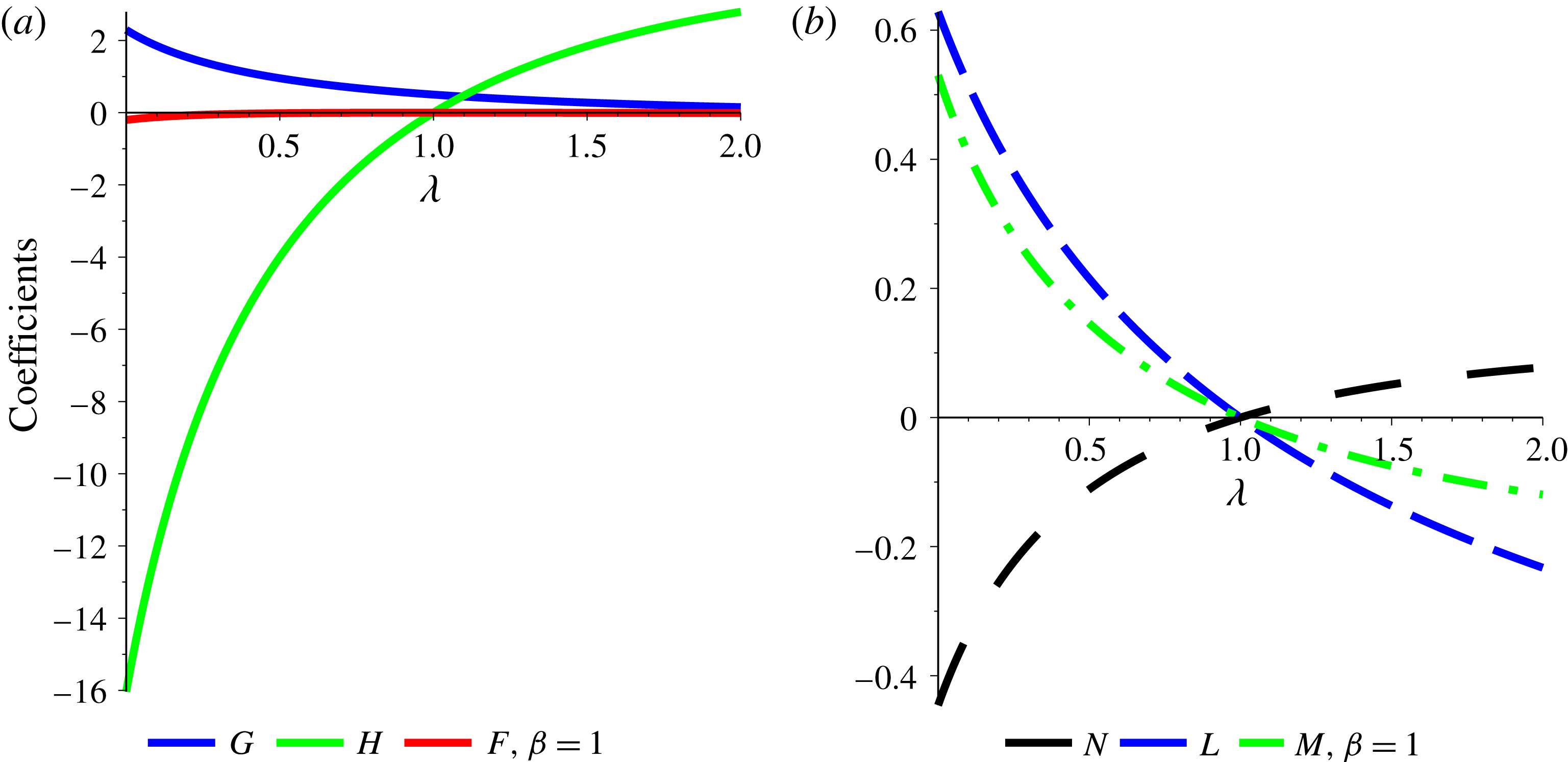
The plots in figure 3 illustrate the dependence of the coefficients on
 $\unicode[STIX]{x1D706}$
. The coefficients for the internal flow are plotted in figure 3(a), while figure 3(b) describes the coefficients for the outer flow. In both series of plots,
 $\unicode[STIX]{x1D6FC}=\unicode[STIX]{x1D702}(\unicode[STIX]{x1D6FD}=1)$
and
 $a=1$
. An important change in the coupled flow takes place at
 $\unicode[STIX]{x1D706}=1$
. All three coefficients for the outer flow become zero at
 $\unicode[STIX]{x1D706}=1$
, indicating that the external flow is described by the imposed infinite flow
 $\boldsymbol{u}^{\infty }=\dot{\unicode[STIX]{x1D640}}\boldsymbol{\cdot }\boldsymbol{r}$
. Such a behaviour in the coupled flow is expected, as the perturbation to the infinite flow is caused by the contrast in the matrix viscosities in the two domains. In the absence of viscosity contrast, the perturbation is removed and flow within both domains is governed by the infinite flow. This situation is similar to previous studies of zeroth-order two-phase flow, in the limit of small time and constant interstitial fluid volume fraction,
 $\unicode[STIX]{x1D719}$
.
Plot of the coefficients for (a) internal and (b) external flow, as a function of
 $\unicode[STIX]{x1D706}$
, the ratio of shear viscosities of the matrices in the sphere and the substrate. In these plots,
 $a=1$
and
 $\unicode[STIX]{x1D6FD}=1$
.

4 The influence of viscosity ratios on coupled flow
4.1 Field variables within both domains
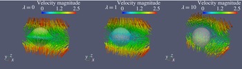
Velocity field within and outside the sphere for three different values of
 $\unicode[STIX]{x1D706}$
. In these visualizations with an imposed pure shear flow, the values of
 $\unicode[STIX]{x1D6FD}$
and
 $a$
are both unity. The colour and length of the vector arrows scale with the magnitude of velocity as shown in the colour bar.

The value of
 $\unicode[STIX]{x1D706}$
exerts a significant influence on the magnitude of velocity within the sphere. The velocity vectors both within and outside the sphere are displayed in figure 4. The colour and length of the vector arrows are proportional to the magnitude of the vectors. For all three visualizations,
 $\unicode[STIX]{x1D6FD}=1$
. The most remarkable feature is the rapid reduction in the magnitude of the internal flow as the value of
 $\unicode[STIX]{x1D706}$
increases from 0 to 10. This behaviour is principally guided by the influence of
 $\unicode[STIX]{x1D706}$
on the coefficients as discussed above. With an increase in the internal viscosity, the magnitude of the flow in the interior of the sphere diminishes. For the value of
 $\unicode[STIX]{x1D706}=1$
, the velocities within and outside the sphere are continuous and are equal to
 $\boldsymbol{u}^{\infty }$
.
(a) Map of pressure
 $p$
within and outside the sphere for
 $\unicode[STIX]{x1D6FD}=1$
,
 $\unicode[STIX]{x1D706}=0$
and
 $a=1$
. The surface of the sphere at the bottom shows the pressure drop at the interface. Only half of the pressure field in the substrate is shown to enable visualization of the sphere. (b) The same as in (a) for
 $\unicode[STIX]{x1D706}=10$
. The colour maps in all four visualizations are scaled according to the colour bars shown.

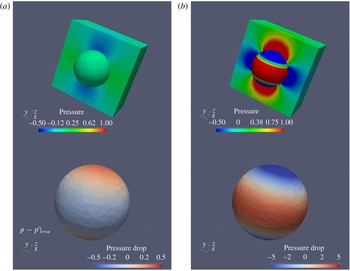
The pressures within and outside the sphere are also strongly modulated by the value of
 $\unicode[STIX]{x1D706}$
. The plots in figure 5 outline the pressure fields within both domains and the pressure difference at the interface. For all of these visualizations,
 $\unicode[STIX]{x1D6FD}=1$
. Two features of the solutions for pressure are evident from these visualizations. First, the magnitude of pressure within the sphere increases with an increase in
 $\unicode[STIX]{x1D706}$
. Second, as a consequence, the difference in pressures at the poles and the equator undergo substantial changes. The bottom panel in both figures illustrates this change, as
 $p-p^{\prime }$
at
 $r=a$
changes sign at both the pole and the equator, in response to an increase in
 $\unicode[STIX]{x1D706}$
. This observation is similar to the observations from the plot in figure 7, described later.
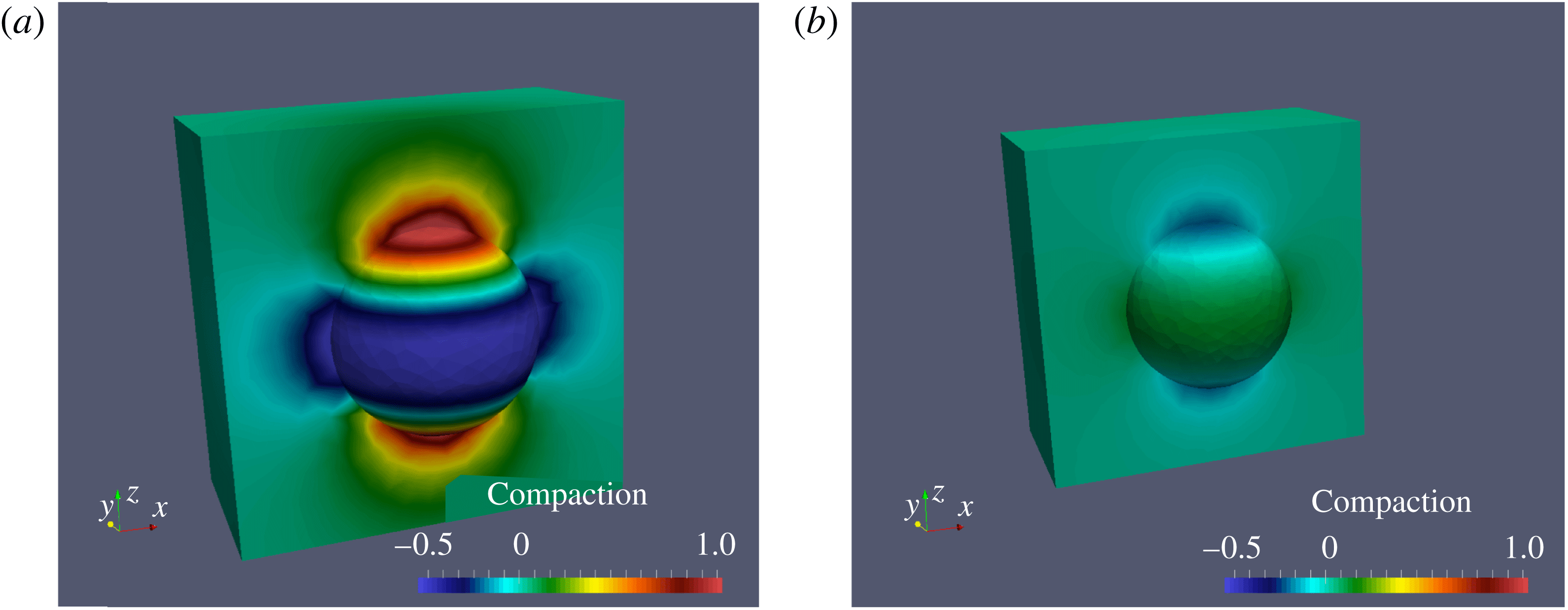
Compactions,
 ${\mathcal{C}}=\unicode[STIX]{x1D735}\boldsymbol{\cdot }\boldsymbol{u}$
, within and outside the sphere are closely related, as shown by the visualization in figure 6. Similar to pressure, compactions within the sphere and the substrate also undergo a change in sign as the value of
 $\unicode[STIX]{x1D706}$
increases from 0 to 1. In addition, the magnitude of the compaction within both domains decreases with an increase in
 $\unicode[STIX]{x1D706}$
, as demonstrated by the intensity of colours in both panels.
The map of compaction within the sphere can also help in understanding the flow of melt within each domain, at least initially. Recall from (3.7) that
 $\text{D}\unicode[STIX]{x1D719}/\text{D}t\approx {\mathcal{C}}$
for small values of
 $\unicode[STIX]{x1D719}$
. Such a zeroth-order approximation is valid only for a very short period of time after the inset of flow. This assumption becomes invalid as deformation progresses within both the sphere and the substrate. Keeping this limitation in mind, we note that the polarity of fluid segregation reverses with a change in the viscosity ratio. For an inviscid sphere matrix, the interstitial fluid collects near the pole of the sphere (
 $\text{D}\unicode[STIX]{x1D719}/\text{D}t>0$
at the pole), while the fluid drains away from the pole when
 $\unicode[STIX]{x1D706}=10$
(
 $\text{D}\unicode[STIX]{x1D719}/\text{D}t<0$
at the pole).
Map of compaction within and outside the sphere for (a)
 $\unicode[STIX]{x1D706}=0$
and (b)
 $\unicode[STIX]{x1D706}=10$
. For both visualizations,
 $\unicode[STIX]{x1D6FD}=1$
. As in figure 5, only half of the substrate is shown. The colour maps within and outside the sphere are scaled according to the colour bars shown.

4.2 The influence of bulk viscosity
The influence of
 $\unicode[STIX]{x1D6FC}=\unicode[STIX]{x1D6FD}\unicode[STIX]{x1D702}$
, the effective bulk viscosity, is unique to multiphase aggregates. As mentioned earlier, even if both the matrix and the interstitial fluid are incompressible, due to the presence of compaction, the two-phase aggregate has a non-zero effective bulk viscosity (McKenzie Reference McKenzie1984; Ricard et al.
Reference Ricard, Bercovici and Schubert2001; Simpson et al.
Reference Simpson, Spiegelman and Weinstein2010a
).
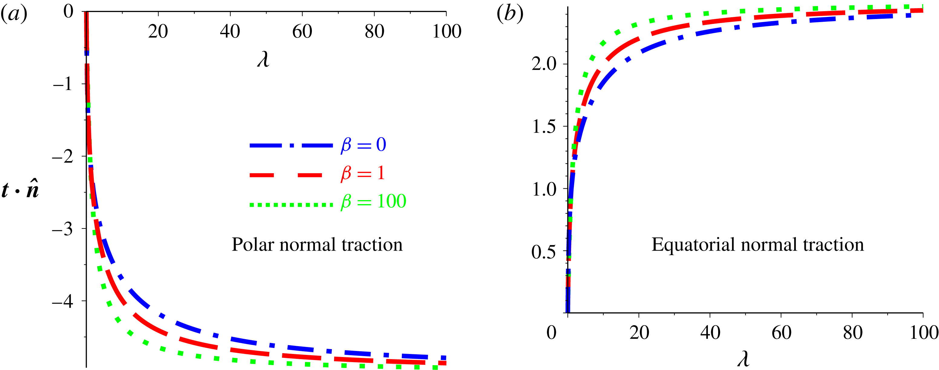
Plots of magnitude of (a) polar (evaluated at
 $x=0$
,
 $y=0$
,
 $z=a$
) and (b) equatorial (evaluated at
 $x=a$
,
 $y=0$
,
 $z=0$
) values of the normal traction as a function of the viscosity ratio,
 $\unicode[STIX]{x1D706}$
, for three different values of
 $\unicode[STIX]{x1D6FD}$
, the ratio between bulk and shear viscosities of the matrix.

The normal component of traction at the interface between the sphere and the substrate shows a nonlinear variation with
 $\unicode[STIX]{x1D706}$
in figure 7. This plot corresponds to the value of
 $\boldsymbol{t}\boldsymbol{\cdot }\hat{\boldsymbol{n}}$
evaluated at the north pole (
 $x=0$
,
 $y=0$
,
 $z=a$
) and at a point on the equator (
 $x=a$
,
 $y=0$
,
 $z=0$
). For a value of
 $\unicode[STIX]{x1D706}=0$
, the inviscid matrix of the inner domain does not support stress, rendering the normal traction zero in both domains. For higher values of
 $\unicode[STIX]{x1D706}$
, the signs of the normal components are opposite at the north pole and at the equator, which are under compression and extension, respectively. As the viscosity of the sphere increases, increasing the value of
 $\unicode[STIX]{x1D706}$
, the magnitudes of both components of the normal traction increase, eventually saturating near a value of
 $\unicode[STIX]{x1D706}=80$
. This observation implies that viscous coupling between the matrices within the sphere and the substrate (as our formulation considers that the fluid phase within each aggregate bears no stress) should saturate at these values of
 $\unicode[STIX]{x1D706}$
. In understanding the viscous coupling between structures in the deep Earth, this limit can be important (Hier-Majumder & Revenaugh Reference Hier-Majumder and Revenaugh2010; Hier-Majumder & Tauzin Reference Hier-Majumder and Tauzin2017). The curves for three different values of
 $\unicode[STIX]{x1D6FD}$
are shown in figure 7. For higher values of
 $\unicode[STIX]{x1D6FD}$
, the increase in the magnitude of normal traction is slightly higher. Compared with the influence of
 $\unicode[STIX]{x1D706}$
, however, the dependence of normal traction on
 $\unicode[STIX]{x1D6FD}$
is weaker.
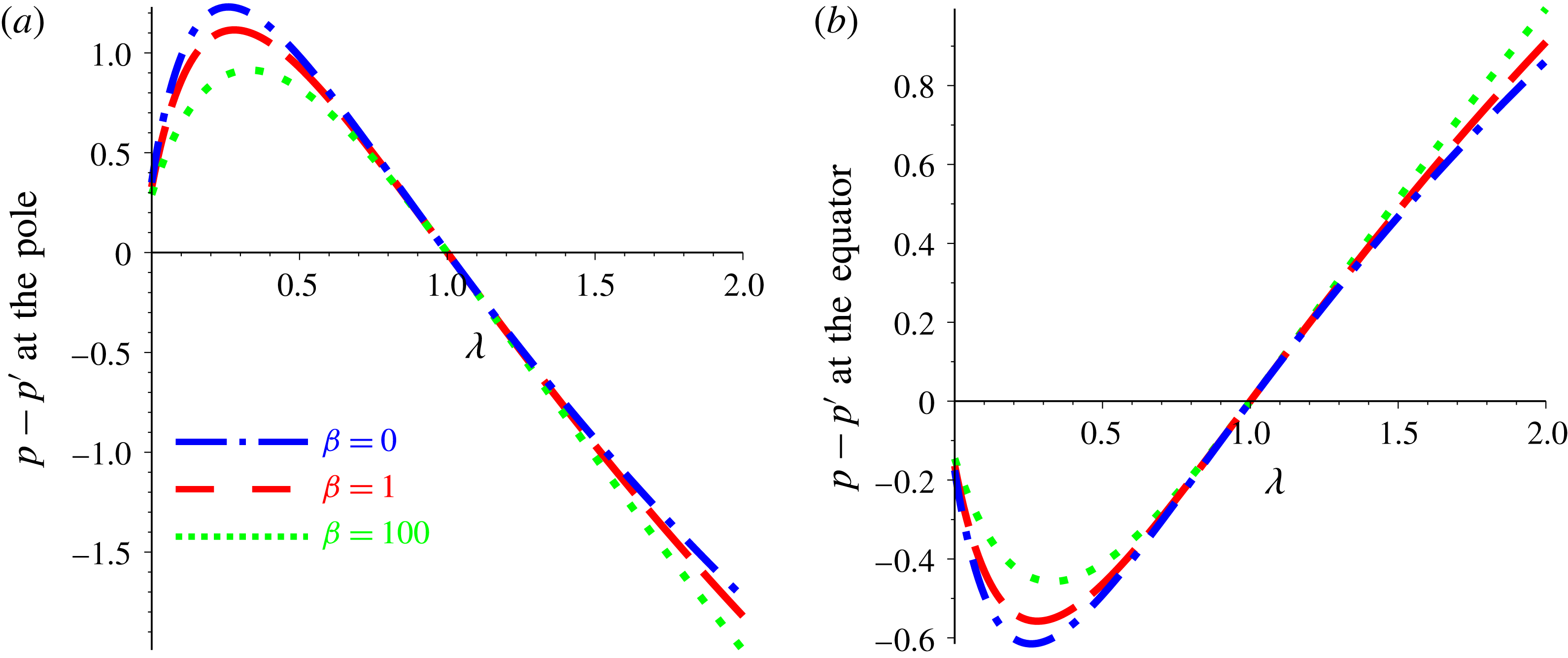
The plots in figure 8 illustrate the variation in
 $p-p^{\prime }$
at
 $r=a$
at the north pole and the equator. Two important features of these plots are the reversal in the sign of
 $p-p^{\prime }$
and the weak dependence on
 $\unicode[STIX]{x1D6FD}$
. For a weak sphere matrix (
 $0<\unicode[STIX]{x1D706}<1$
), the pressure drop displays a maximum and then changes sign as the value of
 $\unicode[STIX]{x1D706}$
increases above unity. When
 $\unicode[STIX]{x1D706}=1$
, flows in both the sphere and the substrate are the same as the imposed far-field flow. In the absence of the perturbation arising from the variations in matrix viscosity, the pressures within both domains are the same, rendering
 $p=p^{\prime }$
when
 $\unicode[STIX]{x1D706}=1$
. Similar to normal traction, the curves display a weak dependence on
 $\unicode[STIX]{x1D6FD}$
as the maximum shifts to a lower value and the position of the maximum shifts to a slightly higher value of
 $\unicode[STIX]{x1D706}$
, as
 $\unicode[STIX]{x1D6FD}$
increases.
Plots of magnitude of polar and equatorial pressure difference between the internal and external fluid (a) at the pole and (b) at the equator as a function of
 $\unicode[STIX]{x1D706}$
, the ratio between matrix viscosities of the sphere and the substrate. As in figure 7, the polar value of
 $p-p^{\prime }$
is evaluated at
 $x=0$
,
 $y=0$
,
 $z=a$
and the equatorial value of
 $p-p^{\prime }$
is evaluated at
 $x=a$
,
 $y=0$
,
 $z=0$
.

5 Discussion and conclusions
The analytical solutions in this article demonstrate the importance of coupling of multiphase flow between two interacting domains. The analytical solutions presented in this work bear important implications for flow magnitude and phase segregation for natural flows. In a recent numerical investigation of coupled flow within the ULVZ and LLSVP system, Hier-Majumder & Drombosky (Reference Hier-Majumder and Drombosky2016) posited that the lower-viscosity ULVZ is strongly deformed by straining flow in the surrounding LLSVP. Owing to the Stokes flow equation used within both domains, however, this work was unable to identify regions of compaction and phase segregation within the ULVZ. The results from the current work support their first conclusion, as the visualizations in figure 4 demonstrate. Additionally, the map of compaction within the spherical domain, shown in figure 6, is now able to provide a zeroth-order approximation of the spatial distribution of compaction and decompaction within the sphere, a first step in understanding the internal structure of the ULVZs. Future work on solution building for a generalized far-field flow will be extremely beneficial for further understanding of such coupled flow. In another recent study of compaction in a one-dimensional melt column within the ULVZ, Hier-Majumder (Reference Hier-Majumder2014) demonstrates that the interstitial melt segregates near the top of the ULVZ during pulsed compaction. The results from this article show that melt segregation will occur near the compressive, polar region of a low-viscosity ULVZ. To fully quantify the segregation of the interstitial fluid, however, it is important to study the coupled two-phase flow in three dimensions. In addition, the extent of fluid segregation will be strongly modulated by the ratio of the matrix shear viscosity of a ULVZ patch and the surrounding mantle.
The results presented in this article suffer from a few limitations resulting from the assumptions. The results focus primarily on the influence of the contrast in matrix shear viscosity within the two domains. In addition to the viscosity ratio,
 $\unicode[STIX]{x1D706}$
, the compaction length,
 $\unicode[STIX]{x1D6FF}$
, within the two domains should also play a significant role in coupling the flow. These solutions assume that the compaction length within domains is the same as the radius of the sphere. This assumption, however, can become invalidated by a number of naturally occurring phenomena. In addition, the mobility of the interstitial fluid can also vary between the two domains, a phenomenon not considered in this article, as we assume these values are the same in both domains. Variations in fluid mobility across the interface will influence the solutions through the boundary conditions for continuity of flux. Such variations will provide additional perturbations to the flow, and the reversal of sign in the pressure and compaction at
 $\unicode[STIX]{x1D706}=1$
may no longer be observed under such conditions. Finally, these analytical solutions are strictly valid for very small time scales following the onset of flow. To fully investigate the nature of the coupled nonlinear flow, future numerical simulations will be extremely helpful.
In conclusion, this article builds the solutions for coupled multiphase, multicomponent flow by decomposing the matrix velocity and reduced fluid pressure within each domain into two scalar functions,
 $\unicode[STIX]{x1D712}$
and
 ${\mathcal{C}}$
, and a vector function,
 $\unicode[STIX]{x1D753}$
. We study the behaviour of the solutions as a function of the ratio of matrix shear viscosities within and outside the sphere. Our results indicate that velocity within the sphere is highest when this ratio is zero, and the magnitude of this velocity drops sharply as the ratio increases. We also note that the magnitudes of the polar and equatorial normal tractions at the surface of the sphere increase from zero to a finite value around
 $\unicode[STIX]{x1D706}=80$
. This indicates that the effective rigidness of the spherical domain is achieved around this value of
 $\unicode[STIX]{x1D706}$
. Finally, we note that the sign of compaction and pressure at the interface between the sphere and the substrate undergoes a change in sign at the poles and the equator, as the viscosity ratio,
 $\unicode[STIX]{x1D706}$
, increases from 0 to 1.
Acknowledgements
The work in this paper was supported by an NSF grant EAR 1215800. The author is extremely grateful for constructive comments by three anonymous reviewers and editor J. Wettlaufer. Software associated with the analytical solution building and visualization is available for download at doi:10.5281/zenodo.838655.
Appendix A. Governing equations
The complete set of governing equations within each domain consists of a mass and momentum conservation equation for each phase supplemented by a set of constitutive equations arising from the conservation of entropy and Onsager’s principle (Bercovici et al. Reference Bercovici, Ricard and Schubert2001a ; Sramek, Ricard & Bercovici Reference Sramek, Ricard and Bercovici2006; Rudge et al. Reference Rudge, Bercovici and Spiegelman2011). For the sake of brevity, the reader is referred to these references for a detailed derivation of the governing equations. Here we present a short derivation of the equations in terms of matrix velocity and reduced fluid pressure. The resultant equations are similar to those obtained by Rudge (Reference Rudge2014).
In the absence of melting or freezing, the equation for conservation of mass of the matrix can be expressed as
 $$\begin{eqnarray}\frac{\unicode[STIX]{x2202}\unicode[STIX]{x1D719}}{\unicode[STIX]{x2202}t}=\unicode[STIX]{x1D735}\boldsymbol{\cdot }((1-\unicode[STIX]{x1D719})\boldsymbol{u}),\end{eqnarray}$$
where
 $\boldsymbol{u}$
is the velocity and
 $1-\unicode[STIX]{x1D719}$
is the volume fraction of the matrix. This equation can be also rewritten as
 $$\begin{eqnarray}\frac{\text{D}\unicode[STIX]{x1D719}}{\text{D}t}=\frac{\unicode[STIX]{x2202}\unicode[STIX]{x1D719}}{\unicode[STIX]{x2202}t}+\boldsymbol{u}\boldsymbol{\cdot }\unicode[STIX]{x1D735}\unicode[STIX]{x1D719}=(1-\unicode[STIX]{x1D719})\unicode[STIX]{x1D735}\boldsymbol{\cdot }\boldsymbol{u}.\end{eqnarray}$$
The material time derivative of the fluid volume fraction on the left-hand side of (A 2) represents the rate of fluid loss or gain from a unit volume of the multiphase aggregate. The unit volumes within each domain are shown in the schematic diagram in figure 1. Since the fluid volume fraction depends on time and space, this derivative is non-zero, rendering the matrix velocity divergent.
Since there are two phases, we need a second equation for conservation of mass of the interstitial fluid, given by
 $$\begin{eqnarray}\unicode[STIX]{x1D735}\boldsymbol{\cdot }(\boldsymbol{u}-\unicode[STIX]{x1D719}\unicode[STIX]{x0394}\boldsymbol{u})=0,\end{eqnarray}$$
where
 $\unicode[STIX]{x0394}\boldsymbol{u}$
is the velocity of segregation between the fluid and the matrix.
In both domains, the matrix acts as the load-bearing unit. As a result, the average normal traction across the sphere–substrate interface will be borne by the matrix on each domain. To evaluate this, we start with the definition of the stress tensor in the matrix,
 $\unicode[STIX]{x1D64F}$
, using the constitutive relation
 $$\begin{eqnarray}\unicode[STIX]{x1D64F}=-[{\textstyle \frac{2}{3}}\unicode[STIX]{x1D702}\unicode[STIX]{x1D735}\boldsymbol{\cdot }\boldsymbol{u}+P_{m}]\unicode[STIX]{x1D644}+\unicode[STIX]{x1D702}\unicode[STIX]{x1D73A}(\boldsymbol{u}),\end{eqnarray}$$
where
 $P_{m}$
is the pressure within the matrix. On the microscopic scale, the representative elementary volume of the partially molten aggregate is occupied by two fluids of distinct physical properties, separated by a clear phase boundary. Under hydrostatic conditions, in the absence of surface tension, the pressures in both phases are equilibrated, i.e.
 $P_{m}=P_{f}$
. Deformation of the viscous matrix, however, leads to a departure from this equilibrium state. Even if both fluid phases are incompressible with a constant density, the pressure difference between the two phases is balanced by the volumetric strain (compaction,
 ${\mathcal{C}}$
) in the matrix. This phenomenon leads to a non-zero bulk viscosity of the aggregate. Note that this bulk viscosity term applies to both phases in the representative elementary volume, not just to one of the constituent phases.
The constitutive equation linking the pressure difference between the matrix and the fluid has been discussed in a number of previous works (McKenzie Reference McKenzie1984; Bercovici et al. Reference Bercovici, Ricard and Schubert2001a ; Simpson et al. Reference Simpson, Spiegelman and Weinstein2010a ; Rudge et al. Reference Rudge, Bercovici and Spiegelman2011). We refer the interested reader to these articles for more information on various notation and techniques used to derive this constitutive equation and Ricard et al. (Reference Ricard, Bercovici and Schubert2001, § 2) for fluid segregation under different conditions of applied stress. Here, we use the constitutive equation proposed by Bercovici et al. (Reference Bercovici, Ricard and Schubert2001a ) and modified by Hier-Majumder et al. (Reference Hier-Majumder, Ricard and Bercovici2006). In the absence of surface tension, the pressure difference between the matrix and the interstitial fluid is balanced by compaction (Bercovici et al. Reference Bercovici, Ricard and Schubert2001a ):
 $$\begin{eqnarray}P_{m}-P_{f}=-\frac{4\unicode[STIX]{x1D702}}{3\unicode[STIX]{x1D719}(1-\unicode[STIX]{x1D719})}\frac{\text{D}\unicode[STIX]{x1D719}}{\text{D}t}=-\frac{4\unicode[STIX]{x1D702}}{3\unicode[STIX]{x1D719}}{\mathcal{C}}.\end{eqnarray}$$
Note that the above definition of the pressure difference between the two phases holds in the absence of mass exchange between the interstitial fluid and the matrix and zero surface tension (Takei & Hier-Majumder Reference Takei and Hier-Majumder2009).
The mass conservation equations are supplemented by two coupled PDEs for momentum conservation. First, the equation for momentum conservation in the matrix is given by
 $$\begin{eqnarray}\unicode[STIX]{x1D735}\left[\frac{4\unicode[STIX]{x1D702}}{3\unicode[STIX]{x1D719}}((1-\unicode[STIX]{x1D719})\unicode[STIX]{x1D735}\boldsymbol{\cdot }\boldsymbol{u})\right]+\unicode[STIX]{x1D735}\boldsymbol{\cdot }\left[\unicode[STIX]{x1D702}(1-\unicode[STIX]{x1D719})\left(\unicode[STIX]{x1D73A}(\boldsymbol{u})-\frac{2}{3}(\unicode[STIX]{x1D735}\boldsymbol{\cdot }\boldsymbol{u})\unicode[STIX]{x1D644}\right)\right]-\frac{1}{\unicode[STIX]{x1D719}}\unicode[STIX]{x1D63E}\boldsymbol{\cdot }\unicode[STIX]{x0394}\boldsymbol{u}=0,\end{eqnarray}$$
where
 $\unicode[STIX]{x1D702}$
is the shear viscosity of the matrix,
 $\unicode[STIX]{x1D644}$
is the unit tensor,
 $\unicode[STIX]{x1D63E}$
is the frictional resistance tensor,
 $\unicode[STIX]{x0394}\boldsymbol{u}$
is the segregation velocity of the interstitial fluid, and the symmetric gradient operator
 $\unicode[STIX]{x1D73A}(\boldsymbol{u})$
is defined as
 $$\begin{eqnarray}\unicode[STIX]{x1D73A}(\boldsymbol{u})=\unicode[STIX]{x1D735}\boldsymbol{u}+(\unicode[STIX]{x1D735}\boldsymbol{u})^{\text{T}}.\end{eqnarray}$$
The first term in (A 6) arises from compaction, the second term from viscous deformation of the matrix, and the last term from friction between the two phases at the phase boundaries within each domain. This force of friction is experienced by both phases in equal and opposite amount (Bercovici et al. Reference Bercovici, Ricard and Schubert2001a ).
Assuming the viscosity of the interstitial fluid is substantially lower than the matrix, we neglect viscous stresses within the fluid. The momentum conservation equation for the fluid then becomes
 $$\begin{eqnarray}-\unicode[STIX]{x1D735}P_{f}-\unicode[STIX]{x1D70C}_{f}\boldsymbol{g}+\frac{1}{\unicode[STIX]{x1D719}}\unicode[STIX]{x1D63E}\boldsymbol{\cdot }\unicode[STIX]{x0394}\boldsymbol{u}=0,\end{eqnarray}$$
where
 $P_{f}$
is the pressure of the interstitial fluid,
 $\unicode[STIX]{x1D70C}_{f}$
is its density and
 $\boldsymbol{g}$
is gravity. Note that (A 8) is a modified version of the Darcy flow equation.
We aim to reduce the system of governing equations to two PDEs in two unknown variables. To achieve this goal, we eliminate
 $\unicode[STIX]{x0394}\boldsymbol{u}$
between (A 3), (A 6) and (A 8). We also define the reduced pressure
 $p$
as
 $$\begin{eqnarray}p=P_{f}+\unicode[STIX]{x1D70C}_{f}gz,\end{eqnarray}$$
leading to the two PDEs in
 $\boldsymbol{u}$
and
 $p$
, within each domain
 $\unicode[STIX]{x1D6FA}_{i}~(i=1,2)$
. Combining (A 4), (A 5) and (A 9), in the absence of gravity, we arrive at the constitutive relation given in (2.6).