1 Introduction
A blast generated by a sudden release of a large amount of energy is a phenomenon of enormous complexity, which involves rapid chemical reactions (such as explosive detonation and afterburn of detonation products), shock waves, interface instability and turbulent mixing, among many others. In order to simplify the analysis, many model problems of blast waves have been proposed in the past, such as the piston approach (the spherical shock wave to be generated by a spherical piston) (Taylor Reference Taylor1946; Whitham Reference Whitham1950), the point-source approach (the blast wave to be induced by a massless point source of energy) (Taylor Reference Taylor1950b ; Sedov Reference Sedov1959) and the finite-source approach (the blast wave is generated by the burst of a high-pressure gas sphere) (Brode Reference Brode1955; Boyer Reference Boyer1960). A comprehensive review of previous research efforts on these blast models was given by Sachdev (Reference Sachdev2004). While the former two blast models are very useful in describing the behaviour of the spherical shock wave; the third one, i.e. the finite-source spherical blast, is the most complex and the closest to reality among the three models (although many simplifications are still made). The present study is focused on the finite-source spherical blast wave. In order to distinguish the present problem from the Taylor–Sedov point-source blast, we refer to it as a ‘finite-source’ spherical blast wave. The present problem has also been called the ‘spherical shock-tube blast’ (Brode Reference Brode1957) due to its similarity to the planar shock-tube problem and as the ‘bursting-sphere blast’ (Zarei & Frost Reference Zarei and Frost2011).
The earliest investigation of the sudden expansion of a sphere of high-pressure gas can be traced back to the analytical efforts of McFadden (Reference McFadden1952), in which he provided an asymptotic solution based on a series expansion about the planar counterpart. In this asymptotic analysis, McFadden only focused on the initial behaviour of the finite-source blast wave. The first attempt to study the overall temporal evolution of the spherical blast-wave structure was made by Brode (Reference Brode1955) through numerical simulation. Afterwards, extensive theoretical, numerical and experimental studies of the problem have been reported in the literature (Brode Reference Brode1959; Boyer Reference Boyer1960; Friedman Reference Friedman1961; Hayes Reference Hayes1968; Lutzky & Lehto Reference Lutzky and Lehto1970; Liu, Khoo & Yeo Reference Liu, Khoo and Yeo1999; Liang, Wang & Chen Reference Liang, Wang and Chen2002; Sachdev Reference Sachdev2004; Zarei & Frost Reference Zarei and Frost2011; Ling, Haselbacher & Balachandar Reference Ling, Haselbacher and Balachandar2011b ; Mankbadi & Balachandar Reference Mankbadi and Balachandar2012).
1.1 Far-field and near-field features
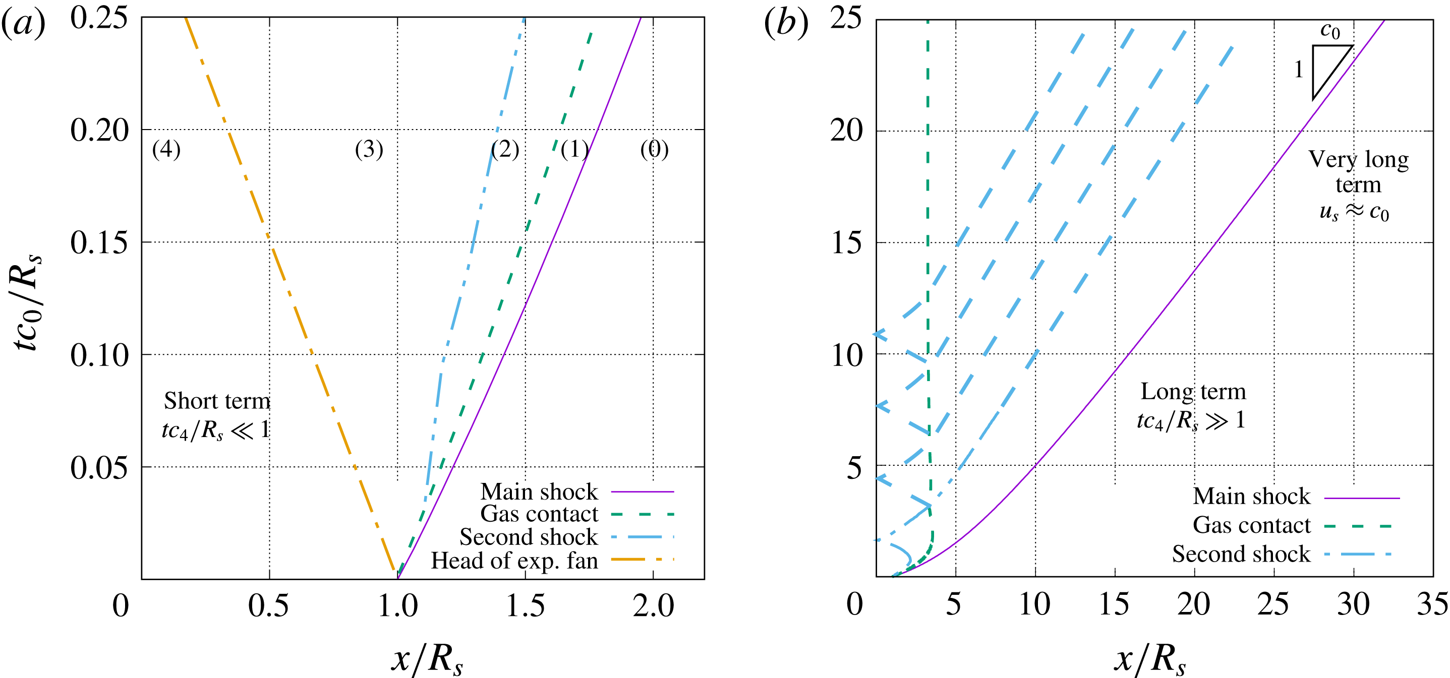
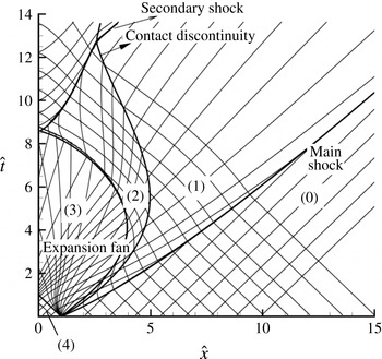
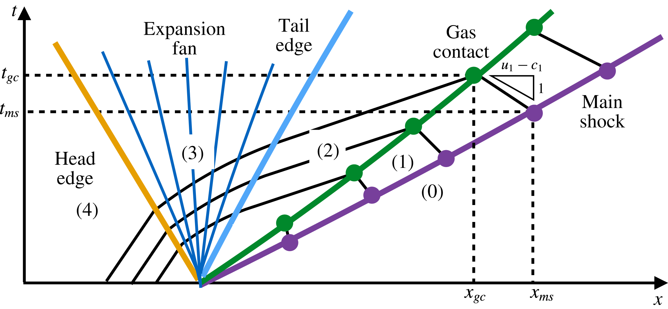
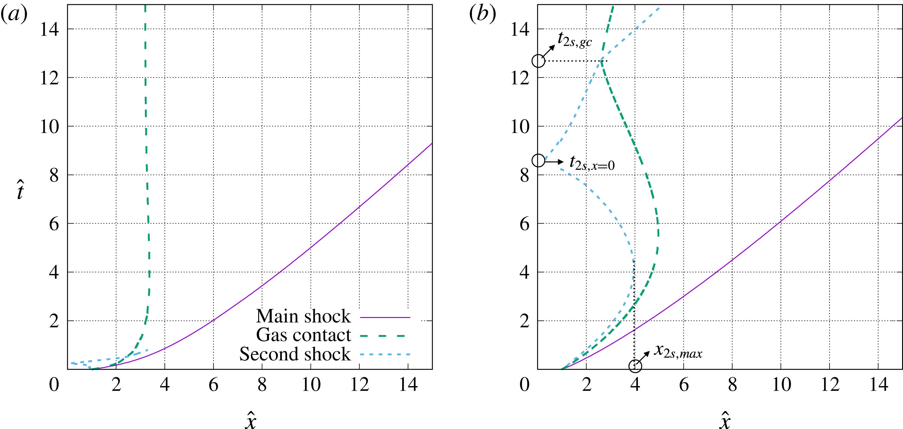
When the spherical blast is initiated, a spherical shock wave and a gas contact surface separating the compressed gas and the ambient air (hereafter referred to as the ‘main shock’ and ‘gas contact’) travel outward; while the head of the expansion fan moves inward into the compressed gas. Typically, the initial pressure inside the sphere is very high, so the gas flow becomes supersonic after passing through the expansion fan and the tail of the expansion fan initially moves outward. The trajectories of these waves are shown in
 $x$
–
 $t$
diagrams in figure 1. Here,
 $x$
is the radial coordinate, and
 $c_{0}$
and
 $R_{s}$
are the speed of sound of the ambient gas and the radius of the sphere (referred to as the ‘charge’), respectively.
The velocities of both the main shock and the gas contact decrease in time. The main shock speed eventually reaches the sound speed in ambiance (i.e. it becomes an acoustic wave), while the gas contact speed decreases to zero. As a result, the shock wave continues to move out and can reach large distances, while the gas contact (and the gas initially contained within the sphere) will remain close to the origin (see figure 1 b). The dynamics of the main shock is considered as the far-field feature (Tyas et al. Reference Tyas, Warren, Bennett and Fay2011) and the gas flow within the gas contact consists of the near field of the blast wave (Balakrishnan, Nance & Menon Reference Balakrishnan, Nance and Menon2010). Compared to the piston and point-source blast-wave models, which are intended to capture the far-field spherical shock dynamics, the finite-source model considered in the present study has the advantage of capturing both the near and far fields, and the formation of the different waves.
Representative
 $x$
–
 $t$
diagrams of the compressible flow induced by a spherical blast for (a) short term and (b) long term.

The near field of a spherical blast has a very complex structure due to multiple wave interactions. A secondary shock forms at the tail of the expansion fan due to the rapid radial expansion or the volumetric effect (Friedman Reference Friedman1961). The secondary shock wave is an imploding shock, but due to the high initial outward gas velocity, the secondary shock is first swept outward before eventually turning inward. The secondary shock is initially weak and its strength increases over time until it reaches the origin, where it is reflected and moves outward. The reflected secondary shock interacts with the gas contact, which generates a reflected tertiary shock and a transmitted secondary shock. Then, a similar cycle starts with the transmitted secondary shock playing the role of the main shock, and the reflected tertiary shock playing the role of the original inward propagating secondary shock. This interaction process continues to create a system of reflected and transmitted shocks that become weaker with each interaction. Through these interactions, the gas bounded by the gas contact continues to expand and compress until it asymptotically approaches a stationary state (Brode Reference Brode1959; Ling et al. Reference Ling, Haselbacher and Balachandar2011b ). These multiple wave interactions can be seen in figure 1(b).
1.2 Short-term and long-term behaviours
The short-term and long-term behaviours of the blast-wave structure are shown in
 $x$
–
 $t$
diagrams in figure 1(a) and 1(b), respectively. The overall domain in the short term is separated into five regions by the four different wave fronts. For convenience of discussion, we number these regions from right to left as shown in figure 1, following the notation of previous works (Friedman Reference Friedman1961; Ling et al.
Reference Ling, Haselbacher and Balachandar2011b
). The different time regimes of the blast-wave development are defined in an asymptotic sense. We define the time scale for the compressed gas within the sphere as
 $$\begin{eqnarray}\unicode[STIX]{x1D70F}_{g}=\frac{R_{s}}{c_{4}},\end{eqnarray}$$
where
 $c_{4}$
is the speed of sound in the compressed gas initially contained within the sphere. Based on this time scale, we present the following definitions of short term and long term and the corresponding flow characteristics:
(i) Short term (
 $t\ll \unicode[STIX]{x1D70F}_{g}$
): In this time regime, the head of the expansion has not yet reached the origin. As a result, the gas flow is not influenced by characteristics reflected from the origin and the speeds of the main shock and the gas contact decrease due to the radial effect only.
(ii) Long term (
$t\gg \unicode[STIX]{x1D70F}_{g}$
): In this time regime, in the near field the secondary shock has already been reflected off the origin and the effect of the finite source dominates the flow evolution. The velocity of the gas contact starts to oscillate as it approaches zero. In the far field, the evolution of the main shock becomes nearly independent of the near-field dynamics and the point-source model becomes appropriate.


1.3 Scaling laws and similarity solutions
As the viscous effect on the blast-wave structure is generally negligible until later stages, the gas motion is governed by the one-dimensional Euler equations in the spherical geometry. Despite the one-dimensional geometry, an analytical solution for the Euler equations is not possible in the spherical geometry. Therefore, a numerical solution, such as the work by Brode (Reference Brode1955), is generally required. With the current numerical techniques and computer power, the one-dimensional Euler equations in the spherical coordinate can be solved to obtain highly accurate numerical solutions (Lutzky & Lehto Reference Lutzky and Lehto1970; Plooster Reference Plooster1970; Igra, Elperin & Ben-Dor Reference Igra, Elperin and Ben-Dor1987; Liang et al.
Reference Liang, Wang and Chen2002; Kato et al.
Reference Kato, Aoki, Kubota and Yoshida2006; Zarei & Frost Reference Zarei and Frost2011; Ling et al.
Reference Ling, Haselbacher and Balachandar2011b
; Mankbadi & Balachandar Reference Mankbadi and Balachandar2012). The two key parameters that control the numerical solutions are the initial pressure ratio (
 $p_{4}/p_{0}$
) between the high-pressure gas and the ambience, and the sound-speed ratio (
 $c_{4}/c_{0}$
). The purpose of the present study is to obtain analytical reductions so that the near-field and far-field features of a finite-source spherical blast wave can be approximately predicted for all values of initial pressure ratio and sound-speed ratio (i.e. for the entire parametric space). Approximate scaling laws and similarity solutions will be presented for both the near-field and far-field features that are appropriate for the short-term and long-term evolution of these features. The significance of these results is that they will allow us to accurately predict quantities of interest such as (i) the time of arrival of the main shock at any point in the ambient air, (ii) the deceleration of the gas contact and the Atwood number of the density jump across the gas contact, both of which are important in obtaining the growth rate of Rayleigh–Taylor instability, (iii) the time of interaction between the contact and the secondary shock, which will initiate the Richtmyer–Meshkov instability of the gas contact.
1.4 Characteristic scales and dimensionless variables
Towards the above objective we introduce a long-term length scale
 ${\mathcal{L}}=R_{s}(p_{4}/p_{0})^{1/3}$
(details will be given later). While, the radius of the spherical charge
 $R_{s}$
is sufficient to characterize the evolution of the blast features in the short term, it is not appropriate for the long-term evolution. The long-term and short-term length scales are defined here as
 $$\begin{eqnarray}\displaystyle & \displaystyle L_{short}=R_{s}, & \displaystyle\end{eqnarray}$$
 $$\begin{eqnarray}\displaystyle & \displaystyle L_{long}={\mathcal{L}}=R_{s}\left(\frac{p_{4}}{p_{0}}\right)^{1/3} & \displaystyle\end{eqnarray}$$
respectively. The numerical results will be used to demonstrate that
 ${\mathcal{L}}$
is the appropriate length scale for both the near-field and far-field features of the spherical blast in the long term.
The temporal evolution of the near-field features (the gas contact and the second shock) are dictated by the sound speed of the compressed gas
 $c_{4}$
, while the velocity scale for the far-field main shock is characterized by the ambient sound speed
 $c_{0}$
, namely
 $$\begin{eqnarray}\displaystyle & \displaystyle V_{near}=c_{4}, & \displaystyle\end{eqnarray}$$
 $$\begin{eqnarray}\displaystyle & \displaystyle V_{far}=c_{0}. & \displaystyle\end{eqnarray}$$
As a result, the characteristic time scales are for different features in different time regimes, namely short-term far field, long-term far field, short-term near field and long-term far field, are different, and can be defined as
 $$\begin{eqnarray}\displaystyle & \displaystyle \unicode[STIX]{x1D70F}_{short-near}=L_{short}/V_{near}=R_{s}/c_{4}, & \displaystyle\end{eqnarray}$$
 $$\begin{eqnarray}\displaystyle & \displaystyle \unicode[STIX]{x1D70F}_{long-near}=L_{long}/V_{near}={\mathcal{L}}/c_{4}, & \displaystyle\end{eqnarray}$$
 $$\begin{eqnarray}\displaystyle & \displaystyle \unicode[STIX]{x1D70F}_{short-far}=L_{short}/V_{far}=R_{s}/c_{0}, & \displaystyle\end{eqnarray}$$
 $$\begin{eqnarray}\displaystyle & \displaystyle \unicode[STIX]{x1D70F}_{long-far}=L_{long}/V_{far}={\mathcal{L}}/c_{0}, & \displaystyle\end{eqnarray}$$
respectively.
The characteristic length, velocity and time scales used for proper scaling of the near-field and far-field blast features for both the short-term and long-term evolution are summarized in table 1. Based on these characteristic scales, different sets of dimensionless variables are defined, as summarized in table 2. As will be shown later in the results, these dimensionless variables are critical to collapsing the results of different cases and developing asymptotic similarity solutions. Here we did not define dimensionless variables for short-term near-field features since there exists no similarity solution. The short-term far-field dimensionless variables,
 $\hat{x},\hat{u} ,\hat{t}$
, will be used in the short-term analysis of near-field features, such as the gas contact.
Summary of characteristic scales in a finite-source spherical blast wave.

Summary of dimensionless variables defined.

1.5 Previous studies on similarity solutions of spherical blast waves
We will first obtain composite scaling laws and similarity solutions for the main shock (far-field feature) that span the entire time evolution taking into account the influence of the near field during the short-term evolution. One of the well-known analytical solutions for spherical blast waves is the Taylor–Sedov blast-wave theory developed in the 1950s by Taylor (Reference Taylor1950b ,Reference Taylor c ) and Sedov (Reference Sedov1959). For a spherical blast wave generated from a point source of energy, a similarity solution for the flow field behind the spherical shock was found. In the original work of Taylor (Reference Taylor1950b ), the spherical shock is considered to be very strong, so that the Rankine–Hugoniot jump conditions can be simplified. The temporal evolution of the spherical shock wave can then be obtained analytically. Extensions of the Taylor–Sedov scaling for moderate shock strength were made by Sakurai (Reference Sakurai1953).
It was shown by Brode (Reference Brode1955) that the main shock in a finite-source spherical blast will reconcile with the point-source solution when the main shock radius is significantly larger than the charge radius (
 $x_{ms}/R_{s}\gg 1$
). However, the short-term evolution of the main shock does not follow the point-source scaling (Brode Reference Brode1955). The physical reason for this discrepancy lies in the different mechanism that controls the short-term evolution of the main shock. In the point-source blast-wave theory, the shock strength decreases due to disturbances from behind the main shock. In the early stages of the finite-source blast, the decay of the spherical main shock is, however, due to the radial effect, or in other words, the increase of the shock surface area. When the shock motion is only dictated by the shock area, the relation between the shock speed and the shock area is governed by the shock-area relation introduced by Whitham (Reference Whitham1958) (also see Chester Reference Chester1954; Chisnell Reference Chisnell1955). The deceleration of the spherical shock due to the shock-area increase is more gradual than that predicted by point-source blast-wave theory (details of scale relations are to be shown later). It was shown by Friedman (Reference Friedman1961) that the shock-area relation well predicts the main shock trajectory in the short term when compared to the numerical results of Brode (Reference Brode1955).
Although the previous analytical works have provided useful scaling relations for the spherical main shock, they are often quite complex and restricted to specific time regimes. Therefore, a comprehensive analysis of the overall temporal evolution of the spherical main shock is desired. It is of present interest to establish a semi-analytical solution for the overall main shock dynamics based on the scaling laws and similarity solutions for the different time regimes.
Most of the previous research efforts have been dedicated to the far field, namely the main shock. Far less attention has been paid to the near-field features such as the gas contact and the secondary shock. Nevertheless, the dynamics of the near-field features and their interactions are often very important. The gas contact will undergo Rayleigh–Taylor (RT) instability (Bell Reference Bell1951; Plesset Reference Plesset1954; Epstein Reference Epstein2004; Mankbadi & Balachandar Reference Mankbadi and Balachandar2012, Reference Mankbadi and Balachandar2013, Reference Mankbadi and Balachandar2014). Also, when the reflected secondary shock overtakes the gas contact, Richtmyer–Meshkov (RM) instability arises (Brouillette Reference Brouillette2002). The development of these instabilities at the gas contact leads to turbulence and mixing between the detonation products and the ambient air, which in turn affects processes such as afterburn of the detonation products (Balakrishnan & Menon Reference Balakrishnan and Menon2010). In the past decade there has been an increasing interest in multiphase blasts where the high-pressure region either contains particles or is surrounded by a spherical bed of particle (Zhang et al. Reference Zhang, Frost, Thibault and Murray2001; Frost et al. Reference Frost, Ornthanalai, Zarei, Tanguay and Zhang2007; Balakrishnan & Menon Reference Balakrishnan and Menon2010; Balakrishnan et al. Reference Balakrishnan, Nance and Menon2010; Ling, Haselbacher & Balachandar Reference Ling, Haselbacher and Balachandar2011a ; Ling et al. Reference Ling, Haselbacher and Balachandar2011b , Reference Ling, Wagner, Beresh, Kearney and Balachandar2012, Reference Ling, Haselbacher, Balachandar, Najjar and Stewart2013; Xu et al. Reference Xu, Lien, Ji and Zhang2013). In the case of a multiphase blast, in addition to the gas contact one also has the particle front across which the density of the gas–particle mixture jumps (the latter is sometimes termed the ‘particle contact’) and therefore becomes unstable like the gas contact (Ukai, Balakrishnan & Menon Reference Ukai, Balakrishnan and Menon2010; Balakrishnan & Menon Reference Balakrishnan and Menon2011; Mankbadi & Balachandar Reference Mankbadi and Balachandar2014). Thus extending the scaling laws and similarity solutions to multiphase blasts is also of importance.
1.6 Goals of the study
In summary, the overarching goal of the present study is to establish asymptotic scaling laws and self-similarity solutions for a finite-source spherical blast wave. The key goals of the present work are to:
(i) Take advantage of the short-term and long-term, strong and weak shock scaling relations to construct an approximate analytical solution for the main shock over the entire time span.
(ii) Develop a simplified asymptotic analysis of the short-term behaviour of the gas contact, and obtain explicit expressions for the deceleration of the gas contact and the Atwood number that characterize the density change across the gas contact.
(iii) Investigate the long-term evolution of the gas contact and obtain appropriate expressions for the asymptotic behaviour.
(iv) Obtain scaling relations for the time of interaction between the secondary shock and the gas contact and investigate the strength of the secondary shock at the time of interaction.
In order to achieve these goals, asymptotic analysis and numerical simulations are performed. We will first present the governing equations and numerical methods in § 2. The simulations will cover a wide range of initial conditions. The results for the main shock, the gas contact and the secondary shock will be presented in sequence in §§ 3–5. In § 3, we will examine the short-term and long-term evolution of the main shock. A long-term length scale that incorporates the initial pressure ratio is introduced and an approximate similarity solution that is independent of the initial condition is presented for the long-term behaviour. With the assistance of the short-term and long-term scaling relations, an overall semi-analytic solution for the main shock dynamics is obtained. In § 4 we will perform an asymptotic analysis of the short-term behaviour of the gas contact, and obtain explicit expressions for the deceleration and the Atwood number of the gas contact. Then, we move on to investigate the long-term evolution and semi-similar behaviour of the gas contact. The time and length scales that characterize the dynamics of the secondary shock are studied and their scaling relations to the initial condition are established in § 5. Finally, we summarize the key findings in § 6.
2 Simulation approach
2.1 Governing equations and numerical methods
In the present study, the blast is considered to occur in an unbounded domain. The gravity effect is neglected. As a result, the gas motion is strictly spherically symmetric at all times. The gas both inside and outside of the sphere is considered to be air and is assumed to follow the ideal gas law. The gas can be treated as inviscid.
The compressible flow is governed by the Euler equations in the spherical geometry,
 $$\begin{eqnarray}\displaystyle & \displaystyle \frac{\unicode[STIX]{x2202}\unicode[STIX]{x1D70C}}{\unicode[STIX]{x2202}t}+\frac{\unicode[STIX]{x2202}\unicode[STIX]{x1D70C}u}{\unicode[STIX]{x2202}x}+2\frac{\unicode[STIX]{x1D70C}u}{x}=0, & \displaystyle\end{eqnarray}$$
 $$\begin{eqnarray}\displaystyle & \displaystyle \frac{\unicode[STIX]{x2202}\unicode[STIX]{x1D70C}u}{\unicode[STIX]{x2202}t}+\frac{\unicode[STIX]{x2202}\unicode[STIX]{x1D70C}u^{2}}{\unicode[STIX]{x2202}x}+2\frac{\unicode[STIX]{x1D70C}u^{2}}{x}=-\frac{\unicode[STIX]{x2202}p}{\unicode[STIX]{x2202}x}, & \displaystyle\end{eqnarray}$$
 $$\begin{eqnarray}\displaystyle & \displaystyle \frac{\unicode[STIX]{x2202}\unicode[STIX]{x1D70C}E}{\unicode[STIX]{x2202}t}+\frac{\unicode[STIX]{x2202}\unicode[STIX]{x1D70C}Hu}{\unicode[STIX]{x2202}x}+2\frac{\unicode[STIX]{x1D70C}Hu}{x}=0, & \displaystyle\end{eqnarray}$$
where
 $\unicode[STIX]{x1D70C}$
,
 $p$
and
 $u$
represent density, pressure and velocity; while
 $E=C_{v}T+u^{2}/2$
, and
 $H=C_{p}T+u^{2}/2$
denote the total energy and the total enthalpy of the gas, where
 $C_{v}$
and
 $C_{p}$
are the specific heat at constant volume and pressure, respectively. Both the compressed gas and air are assumed to obey the ideal gas law,
 $$\begin{eqnarray}p=\unicode[STIX]{x1D70C}RT.\end{eqnarray}$$
The numerical approach for the Euler equations is based on the cell-centred finite-volume methodology. The inviscid flux for the gas is calculated by the approximate Riemann solver of Roe (Reference Roe1981). The face states are obtained by a simplified second-order accurate weighted essentially non-oscillatory scheme, see, e.g. Jiang & Shu (Reference Jiang and Shu1996), which modifies the gradients computed using the least-squares reconstruction method of Barth (Reference Barth1991). The time integration is conducted with the fourth-order Runge–Kutta method. For more details, see Haselbacher (Reference Haselbacher2005), Haselbacher, Balachandar & Kieffer (Reference Haselbacher, Balachandar and Kieffer2007).
2.2 Key parameters
As an initial-value problem, the gas flow at any chosen location and time can be fully determined by the initial condition. The general solution of a quantity of interest,
 $q$
, can be expressed as
 $$\begin{eqnarray}q=q(p_{4},c_{4},\unicode[STIX]{x1D6FE}_{4},p_{0},c_{0},\unicode[STIX]{x1D6FE}_{0},R_{s},x,t),\end{eqnarray}$$
where
 $\unicode[STIX]{x1D6FE}$
represents the specific heat ratio. The subscripts denote the region, i.e.
 $(\,)_{0}$
and
 $(\,)_{4}$
represent properties in regions 0 and 4, as indicated in figure 1(a). If
 $p_{0},c_{0}$
and
 $R_{s}$
are chosen to be the reference variables, then the general solution of the gas flow given in (2.5) can be rewritten in dimensionless form as
 $$\begin{eqnarray}\hat{q}=\hat{q}\left(\frac{p_{4}}{p_{0}},\frac{c_{4}}{c_{0}},\unicode[STIX]{x1D6FE}_{4},\unicode[STIX]{x1D6FE}_{0},\hat{x},\hat{t}\right),\end{eqnarray}$$
where the symbol
 $\hat{()}$
denotes dimensionless variables defined as
 $$\begin{eqnarray}\hat{x}=\frac{x}{R_{s}},\quad \hat{u} =\frac{u}{c_{0}},\quad \hat{t}=\frac{tc_{0}}{R_{s}}.\end{eqnarray}$$
Since
 $R_{s}$
is the only available length scale from geometry, it is natural to use
 $R_{s}$
as the typical length scale, and
 $c_{0}$
, and
 $R_{s}/c_{0}$
are chosen as the characteristic velocity and time scales, respectively (McFadden Reference McFadden1952; Friedman Reference Friedman1961).
Since the specific heat ratios typically vary over a small range, the key dimensionless parameters that control the blast-wave structure are mainly
 $p_{4}/p_{0}$
and
 $c_{4}/c_{0}$
. Since the total energy contained within the compressed gas sphere is
 $$\begin{eqnarray}{\mathcal{E}}_{tot}=\frac{4\unicode[STIX]{x03C0}(R_{s})^{3}p_{4}}{3(\unicode[STIX]{x1D6FE}_{4}-1)},\end{eqnarray}$$
 $p_{4}/p_{0}$
is a measure of the energy released and generally
 $p_{4}/p_{0}\gg 1$
for a blast. The sound-speed ratio
 $c_{4}/c_{0}$
characterizes the difference between the speeds of sound inside and outside of the sphere. Furthermore, assuming the gas to obey the ideal gas equation of state,
 $\unicode[STIX]{x1D70C}=\unicode[STIX]{x1D6FE}p/c^{2}$
, we have
 $\unicode[STIX]{x1D70C}_{4}/\unicode[STIX]{x1D70C}_{0}=(\unicode[STIX]{x1D6FE}_{4}p_{4}/\unicode[STIX]{x1D6FE}_{0}p_{0})/(c_{4}/c_{0})^{2}$
. Therefore, for a given
 $p_{4}/p_{0}$
, the value of
 $c_{4}/c_{0}$
is related to the mass released in a blast. By varying
 $c_{4}/c_{0}$
(or
 $\unicode[STIX]{x1D70C}_{4}/\unicode[STIX]{x1D70C}_{0}$
) the finite-source spherical blast model can be used to approximate blast waves induced by conventional and nuclear explosions. When
 $c_{4}/c_{0}$
is small,
 $\unicode[STIX]{x1D70C}_{4}/\unicode[STIX]{x1D70C}_{0}$
is large, then the blast wave corresponds to a conventional explosion where a substantial mass of gas is released along with energy; while large values of
 $c_{4}/c_{0}$
indicate small
 $\unicode[STIX]{x1D70C}_{4}/\unicode[STIX]{x1D70C}_{0}$
, then the blast wave is similar to that of a nuclear explosion, in which only energy is released.
2.3 Simulation cases
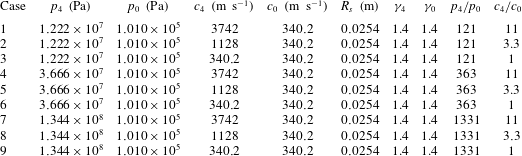
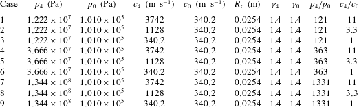
The parameters for different cases simulated are summarized in table 3. The parameters are chosen following the work of Brode (Reference Brode1955). The specific heat ratio
 $\unicode[STIX]{x1D6FE}_{4}=\unicode[STIX]{x1D6FE}_{0}=1.4$
. The ambient air pressure and temperature are taken to be
 $p_{0}=1.01\times 10^{5}$
Pa and
 $T_{0}=288$
K. The speed of sound in the air is then equal to
 $c_{0}=\sqrt{\unicode[STIX]{x1D6FE}_{0}RT_{0}}=340.2~\text{m}~\text{s}^{-1}$
. The pressure and speed of sound of the compressed gas, namely
 $p_{4}$
and
 $c_{4}$
, are varied. (The variation of the speed of sound is due to the change of temperature of the compressed gas.) Three pressure ratios and three sound-speed ratios are considered here. For all cases, the radius of the sphere is taken to be 0.0254 m. Nevertheless, the results in dimensionless variables are independent of the specific value of
 $R_{s}$
.
 $x$
–
 $t$
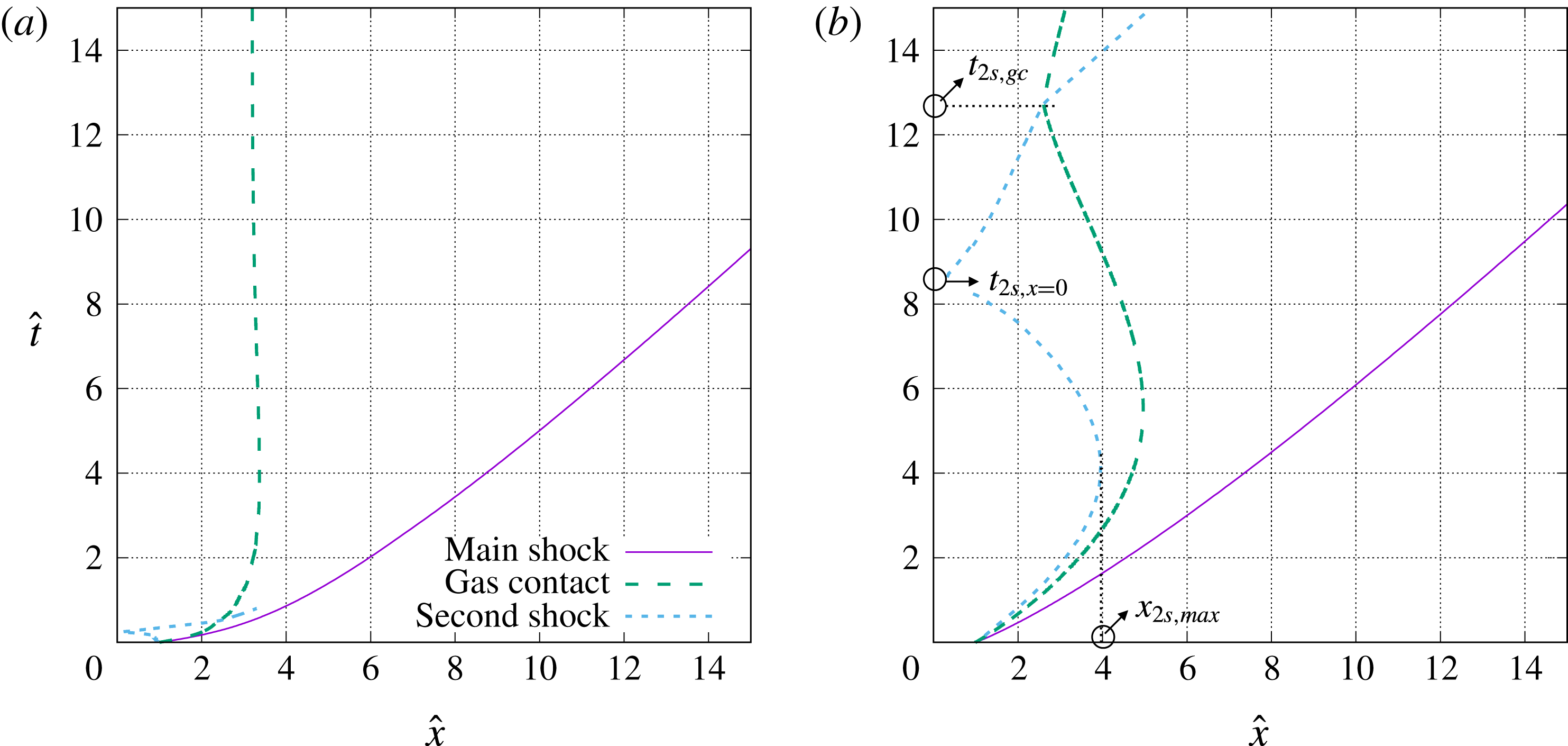
diagrams for cases (a) 1 and (b) 3.
Physical parameters of the gas phase for the cases simulated.
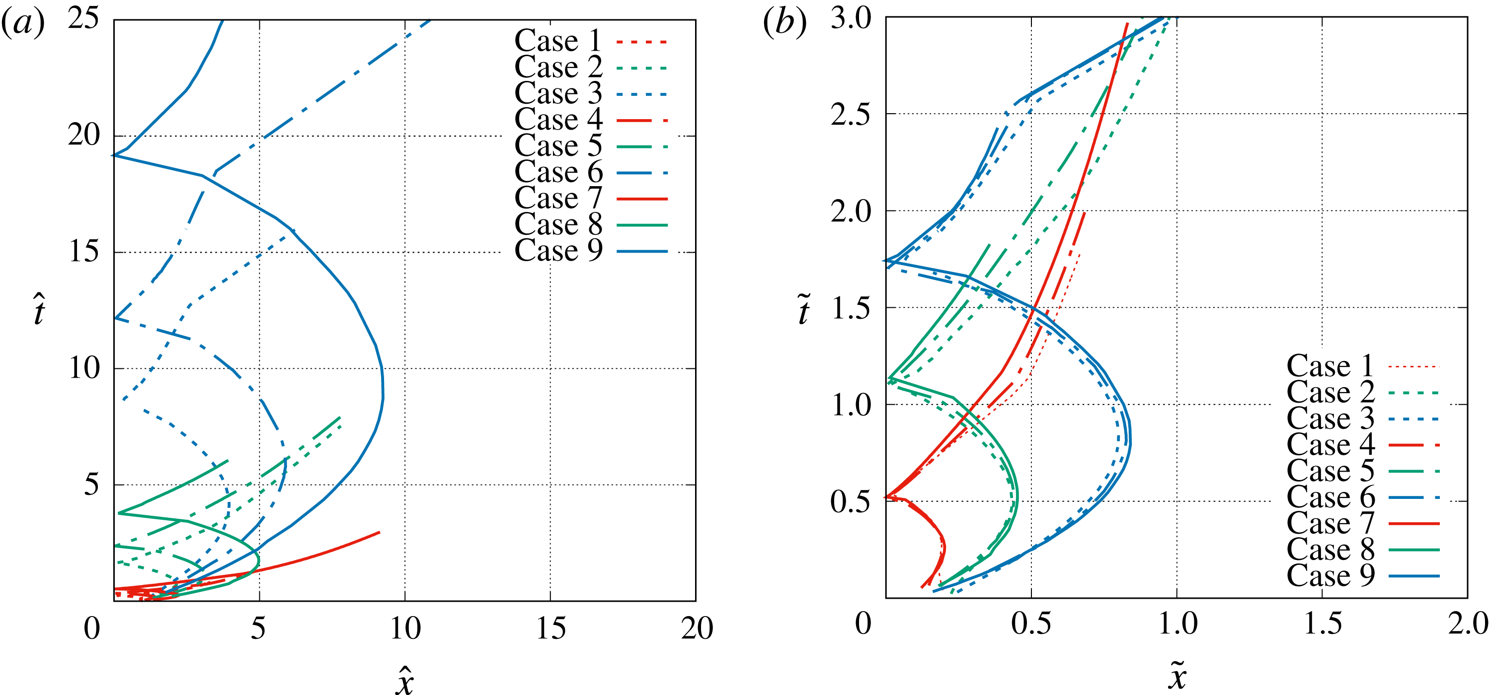
The cases 1 and 3 in table 3 are identical to the cases investigated by Brode (Reference Brode1955). The
 $x$
–
 $t$
diagrams of these two cases are shown in figure 2. While
 $p_{4}$
is the same for the two cases, the temperature ratio between the compressed gas and the ambient air for case 1 is equal to the pressure ratio while that for case 3 is equal to unity. (Brode referred to the cases 1 and 3 as ‘hot sphere’ and ‘cold sphere’). Assuming the air obeys the ideal gas law, the ratio of the speed of sound
 $c_{4}/c_{1}=\sqrt{T_{4}/T_{1}}$
, which can be shown to be higher for case 1 than for case 3. Similarly, the density ratio can also be computed as
 $\unicode[STIX]{x1D70C}_{4}/\unicode[STIX]{x1D70C}_{0}=(p_{4}/p_{0})/(c_{4}/c_{0})^{2}$
, which are equal to 1 and 121 for cases 1 and 3, respectively. Therefore, little gas is released for case 1; while a substantial amount of gas is released for case 3.
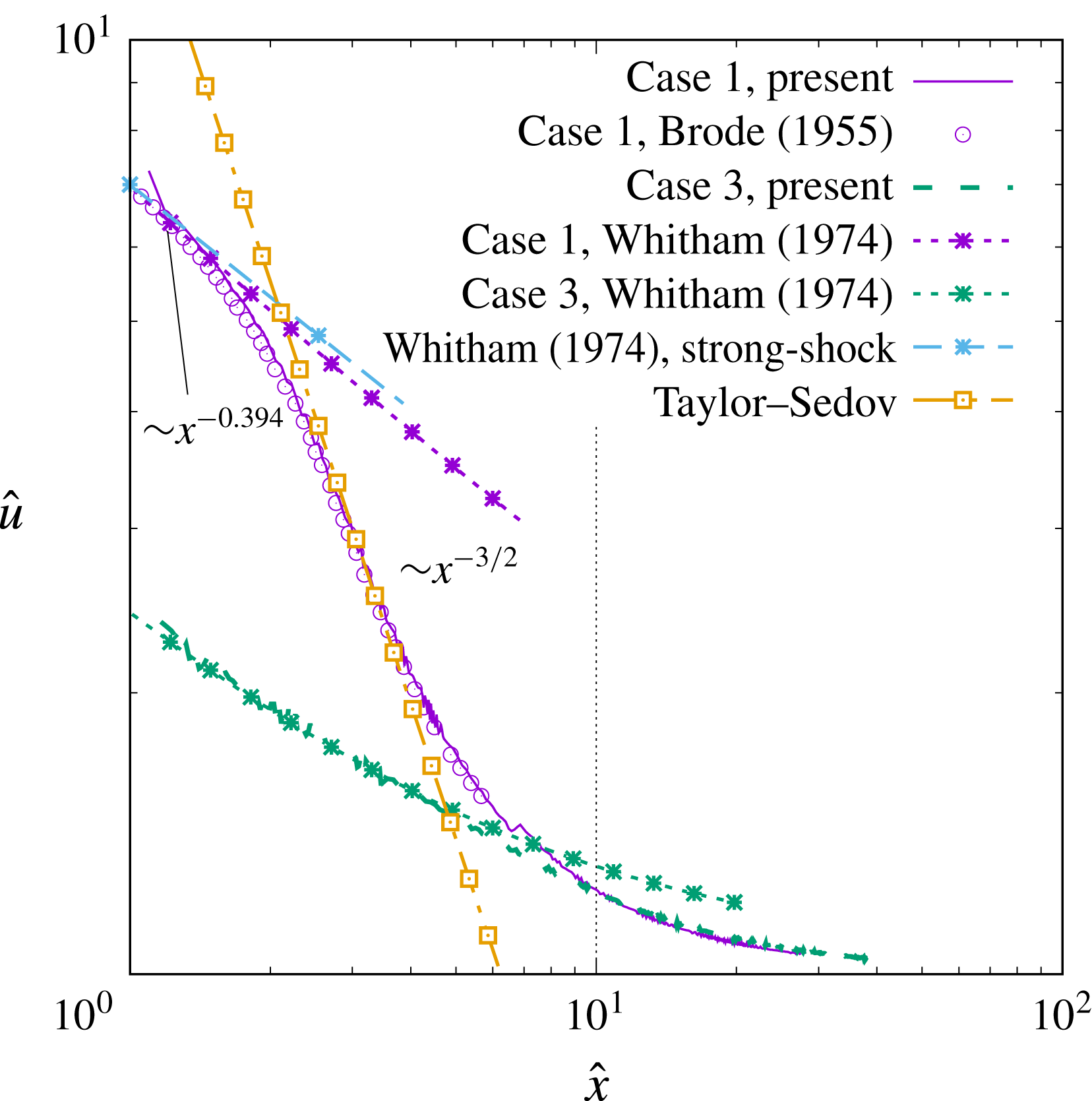
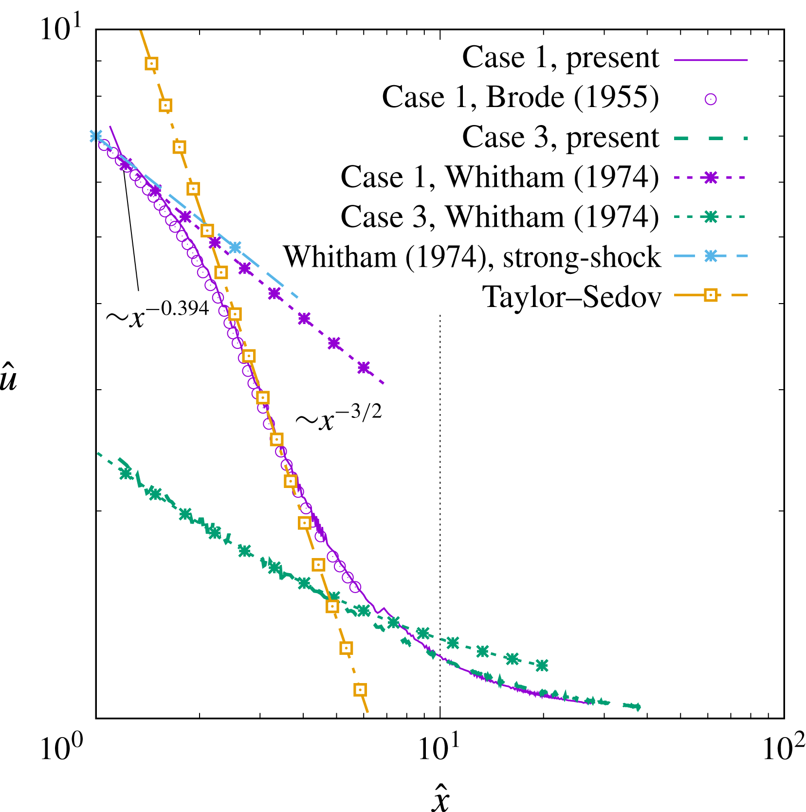
It can be observed that the main shock trajectories for the two cases are quite similar; while those of the gas contact and the secondary shock are very different. The secondary shock reaches the origin at a much earlier time for case 1 than for case 3. The gas contact for case 1 reaches the asymptotic radius monotonically while that for case 3 experiences large-amplitude oscillations. The discrepancy in the near-field solutions between these two cases is clearly due to the different initial speeds of sound within the sphere. Evolutions of the gas contact and the secondary shock are dictated by the positive characteristics from the origin. As information travels much slower in case 3, the velocities of the gas contact and the secondary shock decrease more slowly from their initial values. As a result, there is more time for the gas contact and the secondary shock to reach larger distances before they eventually reverse direction. A comparison of the present result of the speed of the main shock with that of Brode (Reference Brode1955) for the case 1 is shown in figure 3 and good agreement is observed.
Evolution of the speed of the main shock for the case 1 (
 $p_{4}/p_{0}=121$
and
 $c_{4}/c_{0}=11$
) and case 3 (
 $p_{4}/p_{0}=121$
and
 $c_{4}/c_{0}=1$
). The dimensionless variables,
 $\hat{x}$
,
 $\hat{u}$
and
 $\hat{t}$
, are defined in (2.7).
3 Main shock
A general expression for the location and speed of the main shock as a function of time can be expressed in dimensionless form as
 $$\begin{eqnarray}\displaystyle & \displaystyle \hat{x}_{ms}=\unicode[STIX]{x1D709}\left(\frac{p_{4}}{p_{0}},\frac{c_{4}}{c_{0}},\unicode[STIX]{x1D6FE}_{4},\unicode[STIX]{x1D6FE}_{0},\hat{t}\right), & \displaystyle\end{eqnarray}$$
 $$\begin{eqnarray}\displaystyle & \displaystyle \hat{u} _{ms}=\unicode[STIX]{x1D709}^{\prime }\left(\frac{p_{4}}{p_{0}},\frac{c_{4}}{c_{0}},\unicode[STIX]{x1D6FE}_{4},\unicode[STIX]{x1D6FE}_{0},\hat{t}\right). & \displaystyle\end{eqnarray}$$
Here we are interested in finding approximate semi-analytic similarity solutions for
 $\unicode[STIX]{x1D709}$
and
 $\unicode[STIX]{x1D709}^{\prime }$
that appropriately describe the short-term and long-term behaviours.
3.1 Short-term behaviour
The short-term evolution of the main shock follows the shock-area relation of Whitham (Reference Whitham1958). The fundamental idea behind the shock-area relation is that the gas flow properties along a characteristic going to the shock are identical to the properties behind the shock. The shock-area relation of Whitham (Reference Whitham1974) is widely used in the study of shock dynamics due to its ability to predict the behaviour of both diverging and converging shocks. Its limitations have been addressed by Hayes (Reference Hayes1968), who also provided an improved formulation.
As shown in figure 4, the characteristics reaching the main shock from the left are the positive ones and they follow the characteristic equation,
 $$\begin{eqnarray}\text{d}p+\unicode[STIX]{x1D70C}c\,\text{d}u=-\frac{2\unicode[STIX]{x1D70C}c^{2}u}{u+c}\frac{\text{d}x}{x}.\end{eqnarray}$$
Then, by applying the Hugoniot relations to the characteristic equation, the shock-area relation for the main shock can be obtained as
 $$\begin{eqnarray}-\frac{2\,\text{d}x_{ms}}{x_{ms}}=J(M_{ms})\,\text{d}M_{ms},\end{eqnarray}$$
where
 $x_{ms}$
is the radial location of the main shock and
 $M_{ms}$
is the Mach number of the main shock, and the function
 $J$
was given by Friedman (Reference Friedman1961) as
 $$\begin{eqnarray}\displaystyle J(M_{ms}) & = & \displaystyle \left[\frac{4M_{ms}}{2\unicode[STIX]{x1D6FE}_{0}M_{ms}-\unicode[STIX]{x1D6FE}_{0}+1}+\frac{2(M_{ms}^{2}+1)}{M_{ms}\sqrt{[2\unicode[STIX]{x1D6FE}_{0}M_{ms}^{2}-\unicode[STIX]{x1D6FE}_{0}+1][M_{ms}^{2}(\unicode[STIX]{x1D6FE}_{0}-1)+2]}}\right.\nonumber\\ \displaystyle & & \displaystyle \left.+\,\frac{2M_{ms}}{M_{ms}^{2}-1}\sqrt{\frac{(\unicode[STIX]{x1D6FE}_{0}-1)M_{ms}^{2}+2}{2\unicode[STIX]{x1D6FE}_{0}M_{ms}^{2}-\unicode[STIX]{x1D6FE}_{0}+1}}+\frac{M_{ms}^{2}+1}{M_{ms}(M_{ms}^{2}-1)}\right].\end{eqnarray}$$
Numerically generated characteristics of the flow field for case 3.

The initial condition for (3.4) is that
 $x_{ms}/R_{s}=1$
and
 $M_{ms}=M_{ms,pl}$
at
 $t=0$
, where
 $M_{ms,pl}$
is the Mach number of the main shock resulting in a one-dimensional planar shock tube with the same initial pressure and sound-speed ratios
 $p_{4}/p_{0}$
and
 $c_{4}/c_{0}$
, and can be calculated by solving the following implicit planar shock-tube equation,
 $$\begin{eqnarray}\frac{p_{4}}{p_{0}}=\frac{2\unicode[STIX]{x1D6FE}_{0}M_{ms,pl}^{2}-\unicode[STIX]{x1D6FE}_{0}+1}{\unicode[STIX]{x1D6FE}_{0}+1}\left[1-\frac{c_{0}}{c_{4}}\frac{\unicode[STIX]{x1D6FE}_{4}-1}{\unicode[STIX]{x1D6FE}_{0}-1}\frac{M_{ms,pl}^{2}-1}{M_{ms,pl}}\right]^{-(2\unicode[STIX]{x1D6FE}_{4}/\unicode[STIX]{x1D6FE}_{4}-1)}.\end{eqnarray}$$
Then (3.4) can be integrated in time and the results for cases 1 and 3 are shown in figure 3, and compared to the simulation results. It is seen that for the short-term evolution of the main shock, the shock-area theory agrees remarkably well with the numerical results for both cases 1 and 3. For the case 3, the difference between the computed shock speed and the theoretical prediction is almost invisible until
 $\hat{x}_{ms}=5$
(corresponding to
 $\hat{t}=2$
).
Under a strong-shock assumption, i.e.
 $M_{s}\rightarrow \infty$
, equation (3.4) can be simplified as (Whitham Reference Whitham1958)
 $$\begin{eqnarray}-\frac{\text{d}x_{ms}}{x_{ms}}=\frac{\text{d}M_{ms}}{M_{ms}K},\end{eqnarray}$$
which can then be integrated to yield
 $$\begin{eqnarray}M_{ms}=M_{ms,pl}\left(\frac{x_{ms}}{R_{s}}\right)^{-K},\end{eqnarray}$$
where
 $K$
is a function of
 $\unicode[STIX]{x1D6FE}_{0}$
, given as
 $$\begin{eqnarray}K=2\left[\left(1+\sqrt{\frac{2}{\unicode[STIX]{x1D6FE}_{0}(\unicode[STIX]{x1D6FE}_{0}+1)}}\right)\left(1+\sqrt{\frac{2(\unicode[STIX]{x1D6FE}_{0}-1)}{\unicode[STIX]{x1D6FE}_{0}}}\right)\right]^{-1}.\end{eqnarray}$$
Thus, in the limit of a strong shock (i.e.
 $M_{s}\rightarrow \infty$
) the above relation yields the following power law for the shock speed:
 $$\begin{eqnarray}u_{s}\sim x_{s}^{-K}.\end{eqnarray}$$
For
 $\unicode[STIX]{x1D6FE}_{0}=1.4$
,
 $K=0.394$
. This simplified shock-area relation is applied to the case 1 and the result is shown in figure 3. It can be observed that the simplified relation is a good approximation for the full relation for the short term and the agreement with the simulation result is quite good. Since the initial Mach number for the case 3 is small,
 $M_{ms,pl}=2.44$
, the strong-shock simplification is less appropriate for this case.
3.2 Long-term behaviour
3.2.1 Taylor–Sedov solution
As the main shock continues to propagate outward, the weakening effect of perturbations from behind the shock overcomes the effect of the shock-area increase, and as a result the main shock starts to deviate from the shock-area relation prediction and transit to the long-term scaling. The long-term evolution of the main shock was observed to follow well the Taylor–Sedov point-source blast-wave solution, as can be seen for case 1 in figure 3. The point-source blast-wave solution applied to the main shock will yield the following temporal evolution
 $$\begin{eqnarray}x_{s}=S({\mathcal{E}}_{tot}/\unicode[STIX]{x1D70C}_{0})^{1/5}t^{2/5},\end{eqnarray}$$
where
 ${\mathcal{E}}_{tot}$
is the total initial energy contained within the high-pressure sphere (see (2.8)) and
 $S$
is a constant coefficient that only depends on
 $\unicode[STIX]{x1D6FE}_{0}$
. For
 $\unicode[STIX]{x1D6FE}_{0}=1.4$
,
 $S=0.87$
. (The value of
 $S$
here is slightly smaller than the value, 1.03, given by Taylor (Reference Taylor1950c
) as the main shock here does not start from the origin.) The corresponding shock speed can be given as
 $$\begin{eqnarray}u_{s}\sim t^{-3/5}\quad \text{or}\quad u_{s}\sim x_{s}^{-3/2}.\end{eqnarray}$$
The result of the point-source blast-wave theory for case 1 is also shown in figure 3. It is observed that in the time duration when the shock radius
 $\hat{x}_{ms}$
increases from 2.5 to 4, the point-source blast theory agrees well with the simulation result.
Different from case 1, the speed of the main shock never shows a point-source decay rate of
 $x^{-3/2}$
for the case 3. This is due to the fact that the Taylor–Sedov point-source solution is obtained based on the strong-shock assumption, but the main shock for case 3 is relatively weak. In fact, when the Mach number of the main shock is lower than approximately 2, the main shock for case 1 also starts to deviate from the Taylor–Sedov solution and decays in a more gradual manner.
3.2.2 Characteristic length scale for long-term behaviour
For a spherical blast wave generated from a point source, there is no intrinsic length scale from the geometry of the problem. As a result, the only length scale that characterizes the motion of the spherical shock wave is dictated by
 ${\mathcal{E}}_{tot}$
and
 $p_{0}$
, namely,
 $$\begin{eqnarray}{\mathcal{L}}_{ps}\sim \left(\frac{{\mathcal{E}}_{tot}}{p_{0}}\right)^{1/3}.\end{eqnarray}$$
If we take
 ${\mathcal{L}}_{ps}$
as the length scale and continue using the ambient gas speed of sound
 $c_{0}$
as the velocity scale, the Taylor–Sedov solution (3.11) can be rewritten in a dimensionless form as
 $$\begin{eqnarray}\frac{x_{s}}{{\mathcal{L}}_{ps}}=(S\unicode[STIX]{x1D6FE}_{0}^{1/5})\left(\frac{tc_{0}}{{\mathcal{L}}_{ps}}\right)^{2/5}.\end{eqnarray}$$
For a spherical blast from a finite source, in the short term the characteristic length scale is
 $R_{s}$
, but for the long term, the length scale is characterized by the total energy release as in the point-source blast wave. It can be shown that
 $$\begin{eqnarray}\left(\frac{{\mathcal{E}}_{tot}}{p_{0}}\right)^{1/3}=CR_{s}\left(\frac{p_{4}}{p_{0}}\right)^{1/3},\end{eqnarray}$$
where
 $C$
is a constant that depends on
 $\unicode[STIX]{x1D6FE}_{4}$
as
 $$\begin{eqnarray}C=\left[\frac{4\unicode[STIX]{x03C0}}{3(\unicode[STIX]{x1D6FE}_{4}-1)}\right]^{1/3}.\end{eqnarray}$$
Suppressing this dependence on
 $\unicode[STIX]{x1D6FE}_{4}$
we can define a long-term characteristic length scale,
 $$\begin{eqnarray}{\mathcal{L}}=R_{s}\left(\frac{p_{4}}{p_{0}}\right)^{1/3},\end{eqnarray}$$
which incorporates both the charge radius
 $R_{s}$
and the initial pressure ratio
 $p_{4}/p_{0}$
.
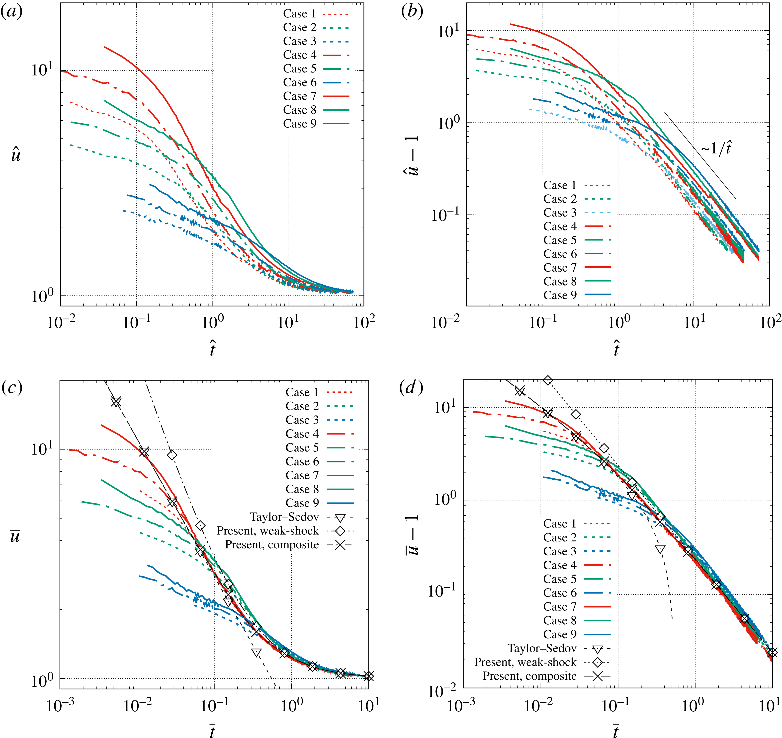
Temporal evolution of the speed of the main shock for different cases (see table 3) and different dimensionless variable: (a) and (b) use
 $\hat{t}=tc_{0}/R_{s}$
and
 $\hat{u} =u/c_{0}$
as the time and velocity scales, while (c) and (d) show the same results with
 $\bar{t}=tc_{0}/{\mathcal{L}}$
and
 $\bar{u}=u/c_{0}$
as the time and velocity scales.

3.2.3 Long-term similarity solution for strong shocks
The temporal evolution of the main shock for cases listed in table 3 are shown in figure 5. If we use
 $R_{s}$
as the characteristic length scale and plot
 $u_{ms}/c_{0}$
as a function of
 $tc_{0}/R_{s}$
, then, as shown in figure 5(a), the results are quite different from case to case. If we use the length scale
 ${\mathcal{L}}=R_{s}(p_{4}/p_{0})^{1/3}$
, (with the velocity scale
 $c_{0}$
remaining unchanged), then it is interesting to observe that the results for all cases collapse remarkably well after an early period of transition, see figure 5(c). This indicates that an asymptotic similarity solution exists for the main shock in the long term. Similar long-term self-similar behaviour has also been observed also by Brode (Reference Brode1955) and Lutzky & Lehto (Reference Lutzky and Lehto1970) for the overpressure of the main shock as a function of shock radius.
Assuming the effect of specific heat ratio is small, we can rewrite (3.1) and (3.2) in a self-similar form as
 $$\begin{eqnarray}\displaystyle & \displaystyle \bar{x}_{ms}=\unicode[STIX]{x1D709}_{sim}(\bar{t}), & \displaystyle\end{eqnarray}$$
 $$\begin{eqnarray}\displaystyle & \displaystyle \bar{u}_{ms}=\unicode[STIX]{x1D709}_{sim}^{\prime }(\bar{t})\quad \text{for }\bar{t}\,\gtrsim \,\bar{t}_{sim}, & \displaystyle\end{eqnarray}$$
where the dimensionless variables are defined as
 $$\begin{eqnarray}\bar{x}=\frac{x}{{\mathcal{L}}},\quad \bar{u}=\frac{u}{c_{0}},\quad \bar{t}=\frac{tc_{0}}{{\mathcal{L}}}.\end{eqnarray}$$
It can be observed that the time taken by the main shock to approach the similarity solution, i.e.
 $\bar{t}_{sim}$
, varies with the initial condition,
 $p_{4}/p_{0}$
and
 $c_{4}/c_{0}$
. However, the self-similar solution
 $\unicode[STIX]{x1D709}_{sim}^{\prime }$
itself does not depend on the initial pressure and sound-speed ratios. It is observed that
 $\bar{t}_{sim}$
decreases when
 $p_{4}/p_{0}$
or
 $c_{4}/c_{0}$
increases. A close examination of the transition time for the main shock to self-similarity solution shows that, for all the cases considered here,
 $t_{sim}$
is between approximately 1.5 and
 $2.5R_{s}/c_{4}$
, approximately twice the time for the head of the expansion fan to reach the origin.
For cases with a larger
 $c_{4}/c_{0}$
, the shock speed merges to the similarity solution earlier and then decays following the Taylor–Sedov scaling
 ${\sim}t^{-3/5}$
. By fitting the data, the multiplicative coefficient can be found to be 0.7, so the similarity solution when the shock remains strong can be expressed as
 $$\begin{eqnarray}\unicode[STIX]{x1D709}_{sim}^{\prime }(\bar{t})=0.7(\bar{t})^{-3/5}\quad \text{for }\bar{u}_{ms}\,\gtrsim \,2\text{ or }\bar{t}\lesssim 0.2.\end{eqnarray}$$
The main shock becomes weaker as it continues to propagate outward, the strong-shock assumption in the Taylor–Sedov solution is not valid and the shock speed deviates from (3.21), decaying more gradually. Sakurai (Reference Sakurai1953) has extended the Taylor–Sedov solution to lower shock strength. Yet the extension is only valid to moderate shock Mach number. For a very weak spherical shock, Whitham (Reference Whitham1950) obtained a solution for the temporal evolution of the main shock based on a correction to the linear theory.
3.2.4 Long-term similarity solution for weak shocks
In order to find the expression for
 $\unicode[STIX]{x1D709}_{sim}^{\prime }$
for the very long term when the main shock becomes weak, i.e. for
 $\bar{t}\,\gtrsim \,0.2$
or
 $\bar{u}_{ms}\lesssim 2$
, the evolution of
 $u_{ms}/c_{0}-1$
is shown in figure 5(b) and (d). As the main shock will eventually turn into a sound wave,
 $u_{ms}/c_{0}\rightarrow 1$
for
 $t\rightarrow \infty$
. It is observed that when the main shock is weak,
 $u_{ms}/c_{0}-1$
follows a
 $t^{-1}$
scaling for all cases. By fitting the data, it can be found that
 $$\begin{eqnarray}\unicode[STIX]{x1D709}_{sim}^{\prime }(\bar{t})=1+0.24(\bar{t})^{-1}\quad \text{for }\bar{u}_{ms}\lesssim 2\text{ or }\bar{t}\,\gtrsim \,0.2.\end{eqnarray}$$
3.3 A composite model for the main shock evolution
Using weighting functions we can connect the strong-shock and weak-shock expressions in (3.21) and (3.22) and build an approximate composite model for
 $\unicode[STIX]{x1D709}_{sim}^{\prime }$
as
 $$\begin{eqnarray}\bar{u}_{ms}=\unicode[STIX]{x1D709}_{sim}^{\prime }(\bar{t})=0.7(\bar{t})^{-3/5}w_{1}(\bar{t})+\left[1+0.24(\bar{\bar{t}})^{-1}\right]w_{2}(\bar{t})\quad \text{for }\bar{t}\,\gtrsim \,\bar{t}_{sim},\end{eqnarray}$$
where the weighting functions are defined as
 $$\begin{eqnarray}\displaystyle \left.\begin{array}{@{}c@{}}\displaystyle w_{1}(\bar{t})=\frac{\exp (-\bar{t}/0.2)}{\exp (-\bar{t}/0.2)+\exp (-0.2/\bar{t})},\\ \displaystyle w_{2}(\bar{t})=\frac{\exp (-0.2/\bar{t})}{\exp (-\bar{t}/0.2)+\exp (-0.2/\bar{t})}.\end{array}\right\} & & \displaystyle\end{eqnarray}$$
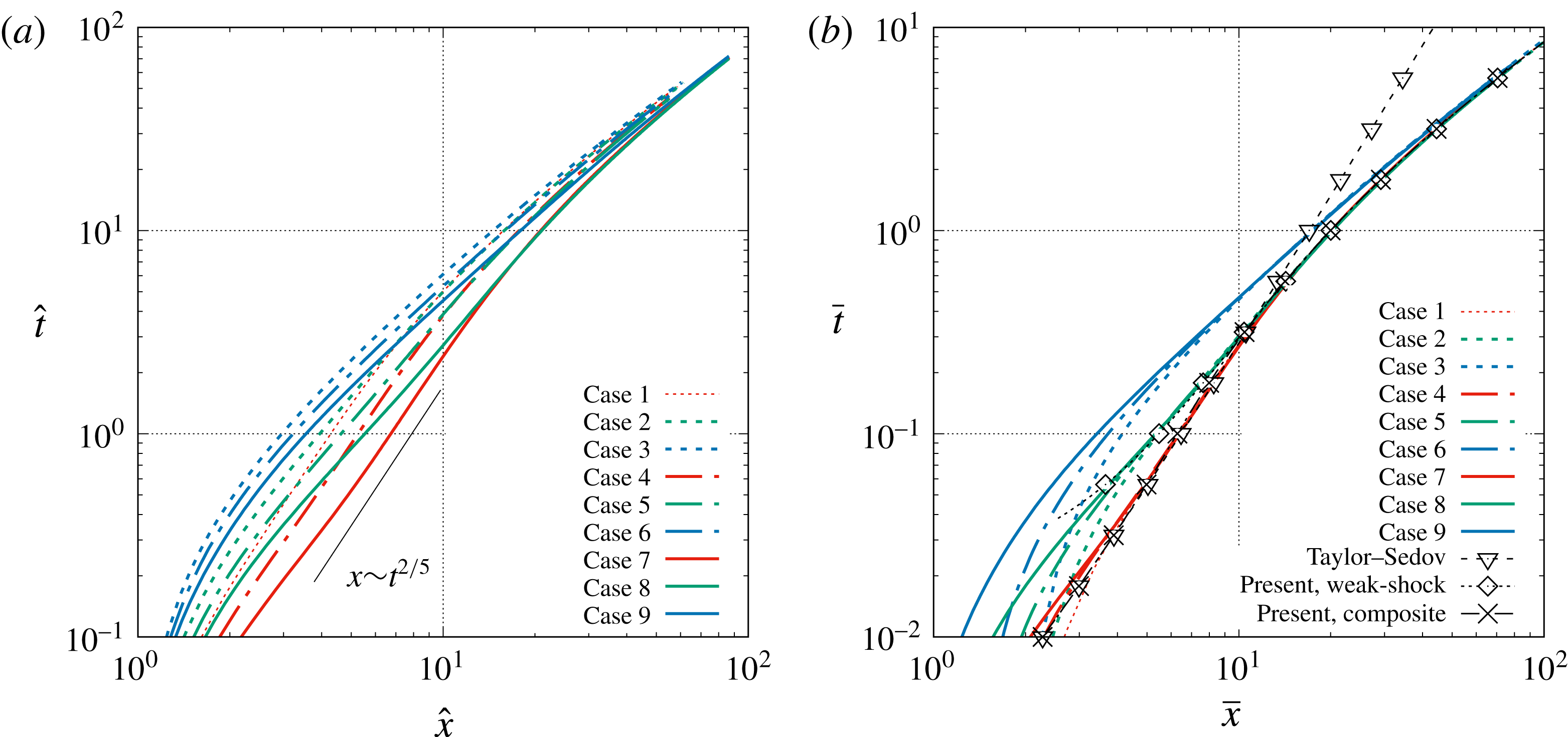
The result of the composite model is shown in figure 5(c,d) and a good agreement with the simulation results is achieved. With a similar procedure, a composite expression for
 $\bar{x}_{ms}$
can also be obtained as
 $$\begin{eqnarray}\bar{x}_{ms}=\unicode[STIX]{x1D709}_{sim}(\bar{t})=\left[1.75(\bar{t})^{2/5}-0.05\right]w_{1}(\bar{t})+\left[0.24\ln (\bar{t})+\bar{t}+1\right]w_{2}(\bar{t})\quad \text{for }\bar{t}\,\gtrsim \,\bar{t}_{sim},\end{eqnarray}$$
and the corresponding comparison with the simulation results are given in figure 6.
Trajectories of the main shock for different cases (a) with
 $\hat{x}=x/R_{s}$
and
 $\hat{t}=tc_{0}/R_{s}$
as the length and time scales and (b) with
 $\bar{x}=x/{\mathcal{L}}$
and
 $\bar{t}=tc_{0}/{\mathcal{L}}$
as the length and time scales.

With the similarity solution (3.23)–(3.25) and the shock-area relation of Whitham (3.4), one can describe the main shock velocity evolution semi-analytically. The steps are summarized here:
(i) With given initial pressure and sound-speed ratios (i.e.
$p_{4}/p_{0}$
and
$c_{4}/c_{0}$
) solve the planar shock-tube problem, namely (3.6), to get the initial velocity of the main shock,
$u_{ms}(t=0)=u_{ms,pl}$
.(ii) With this initial condition, integrate Whitham’s shock-area relation (3.4) and (3.5) to get the short-term evolution.
(iii) Use the similarity solution in (3.23) for long-term evolution of the main shock.
(iv) Connecting the short-term and long-term results obtained in steps (ii) and (iii) with weighting functions similar to those given (3.24).



One can scale the results back to dimensional form with the characteristic scales defined in (3.17) and (3.20). With the shock speed or shock Mach number, the shock overpressure and other post-shock gas properties can be obtained from the Rankine–Hugoniot conditions.
4 Gas contact
Similar to (3.1) and (3.2) for the main shock, the general solution for the location and speed of the gas contact can be written as
 $$\begin{eqnarray}\displaystyle & \displaystyle \hat{x}_{gc}=\unicode[STIX]{x1D701}\left(\frac{p_{4}}{p_{0}},\frac{c_{4}}{c_{0}},\unicode[STIX]{x1D6FE}_{4},\unicode[STIX]{x1D6FE}_{0},\hat{t}\right), & \displaystyle\end{eqnarray}$$
 $$\begin{eqnarray}\displaystyle & \displaystyle \hat{u} _{gc}=\unicode[STIX]{x1D701}^{\prime }\left(\frac{p_{4}}{p_{0}},\frac{c_{4}}{c_{0}},\unicode[STIX]{x1D6FE}_{4},\unicode[STIX]{x1D6FE}_{0},\hat{t}\right). & \displaystyle\end{eqnarray}$$
Before we investigate the long-term evolution of the gas contact we will first study the short-term behaviour when the gas contact decelerates from its initial velocity. Unlike the main shock, the gas contact reaches an asymptotic radius as
 $\hat{t}\rightarrow \infty$
. The dependence of the gas contact on initial pressure and sound-speed ratios will be studied.
4.1 Short-term behaviour
4.1.1 Asymptotic solution at
$t=0^{+}$

Immediately after the bursting of the diaphragm, the characteristic wave corresponding to the gas contact instantly forms. At time zero, the velocity of the gas contact and the Atwood number at the gas contact are the same as those for the corresponding planar shock-tube analogue (i.e. for the planar shock tube with the same initial pressure and density difference across the diaphragm). The Atwood number is defined as
 $$\begin{eqnarray}\mathit{At}_{gc}=\frac{\unicode[STIX]{x1D70C}_{gc,2}-\unicode[STIX]{x1D70C}_{gc,1}}{\unicode[STIX]{x1D70C}_{gc,2}+\unicode[STIX]{x1D70C}_{gc,1}}.\end{eqnarray}$$
In other words, at
 $t=0^{+}$
, the formation of different waves is independent of the planar, cylindrical or spherical geometry of the problem. Note that the gas contact is a material front and thus its velocity is the same as the gas velocity. Thus,
 $$\begin{eqnarray}\displaystyle \hat{u} _{gc,t=0^{+}}=\hat{u} _{gc,pl}=\hat{u} _{1,pl}, & & \displaystyle\end{eqnarray}$$
where
 $\hat{u} _{1,pl}$
is the uniform gas velocity in region 1 (see figure 1) as obtained for the planar shock tube (in the planar problem this velocity is the same as the uniform velocity in region 2, since there is no velocity jump across the gas contact). Similarly, every other gas property, such as gas density, speed of sound, etc., on either side of the gas contact at
 $\hat{t}=0^{+}$
can be obtained from the planar shock-tube solution. Then the Atwood number at
 $t=0^{+}$
can be expressed as
 $$\begin{eqnarray}\displaystyle \mathit{At}_{gc,t=0+}=\mathit{At}_{gc,pl}=\frac{\unicode[STIX]{x1D70C}_{2,pl}-\unicode[STIX]{x1D70C}_{1,pl}}{\unicode[STIX]{x1D70C}_{2,pl}+\unicode[STIX]{x1D70C}_{1,pl}}. & & \displaystyle\end{eqnarray}$$
However, unlike in the planar case where the gas contact moves with a constant speed, in the spherical geometry, as the gas contact moves radially out, its velocity decreases. This deceleration of the gas contact is similar to the short-term deceleration of the main shock that we discussed earlier. As a result, the deceleration of the gas contact at
 $t=0^{+}$
is non-zero and the deceleration cannot be obtained from the planar shock-tube theory (since gas contact moves at constant velocity in a planar shock tube). Similarly, other gas properties also show a slow short-term variation from their initial planar values. In particular, the strength of the density jump across the gas contact, as quantified by the Atwood number, changes in time and the value of
 $\text{d}\mathit{At}_{gc}/\text{d}t|_{t=0^{+}}$
can be evaluated by taking into account the radial effect. The deceleration of the heavy-to-light density front (
 $\mathit{At}_{gc}>0$
) at the gas contact results in the Rayleigh–Taylor (RT) instability (Rayleigh Reference Rayleigh1883; Taylor Reference Taylor1950a
), the growth rate of which depends on the magnitude of deceleration and the Atwood number. Here we will obtain approximate analytical solutions for both the deceleration and the Atwood number of the gas contact in the asymptotic limit of
 $t=0^{+}$
.
The full asymptotic solution for a spherical blast wave at
 $t=0^{+}$
was given by McFadden (Reference McFadden1952). Since the flow in the planar shock tube is self-similar, McFadden introduced the dimensionless variables
 $$\begin{eqnarray}\displaystyle q=\frac{\unicode[STIX]{x1D6FE}-1}{\unicode[STIX]{x1D6FE}+1}\left[\frac{2}{\unicode[STIX]{x1D6FE}-1}+\frac{1-\hat{x}}{{\hat{c}}_{4}\hat{t}}\right],\quad y={\hat{c}}_{4}\hat{t}, & & \displaystyle\end{eqnarray}$$
which are the self-similar variables for
 $\hat{x}$
and
 $\hat{t}$
. The planar shock-tube solution then only depends on
 $q$
, e.g.
 $\hat{u} _{pl}=\hat{u} _{pl}(q)$
. The velocity, speed of sound and density in the spherical blast wave can be expressed in a series expansion about the planar shock-tube solution
 $$\begin{eqnarray}\displaystyle & \displaystyle \hat{u} (q,y)=\hat{u} _{pl}(q)+\frac{\text{d}\hat{u} }{\text{d}y}y+O(y^{2}), & \displaystyle\end{eqnarray}$$
 $$\begin{eqnarray}\displaystyle & \displaystyle {\hat{c}}(q,y)={\hat{c}}_{pl}(q)+\frac{\text{d}{\hat{c}}}{\text{d}y}y+O(y^{2}), & \displaystyle\end{eqnarray}$$
 $$\begin{eqnarray}\displaystyle & \displaystyle \hat{\unicode[STIX]{x1D70C}}(q,y)=\hat{\unicode[STIX]{x1D70C}}_{pl}(q)+\frac{\text{d}\hat{\unicode[STIX]{x1D70C}}}{\text{d}y}y+O(y^{2}), & \displaystyle\end{eqnarray}$$
where
 ${\hat{c}}=c/c_{0}$
and
 $\hat{\unicode[STIX]{x1D70C}}=\unicode[STIX]{x1D70C}/(p_{0}/c_{0}^{2})$
. For small
 $\hat{t}$
or
 $y$
, higher-order terms are dropped. The first-order terms in different regions can be solved analytically using the flow conditions at the waves as boundary conditions to yield the first-order spherical correction to the planar solution. The coefficients of the first-order terms,
 $\text{d}\hat{u} /\text{d}y$
,
 $\text{d}{\hat{c}}/\text{d}y$
and
 $\text{d}\hat{\unicode[STIX]{x1D70C}}/\text{d}y$
, for case 1 (
 $p_{4}/p_{0}=121$
,
 $c_{4}/c=11$
) and case 3 (
 $p_{4}/p_{0}=121$
,
 $c_{4}/c_{0}=1$
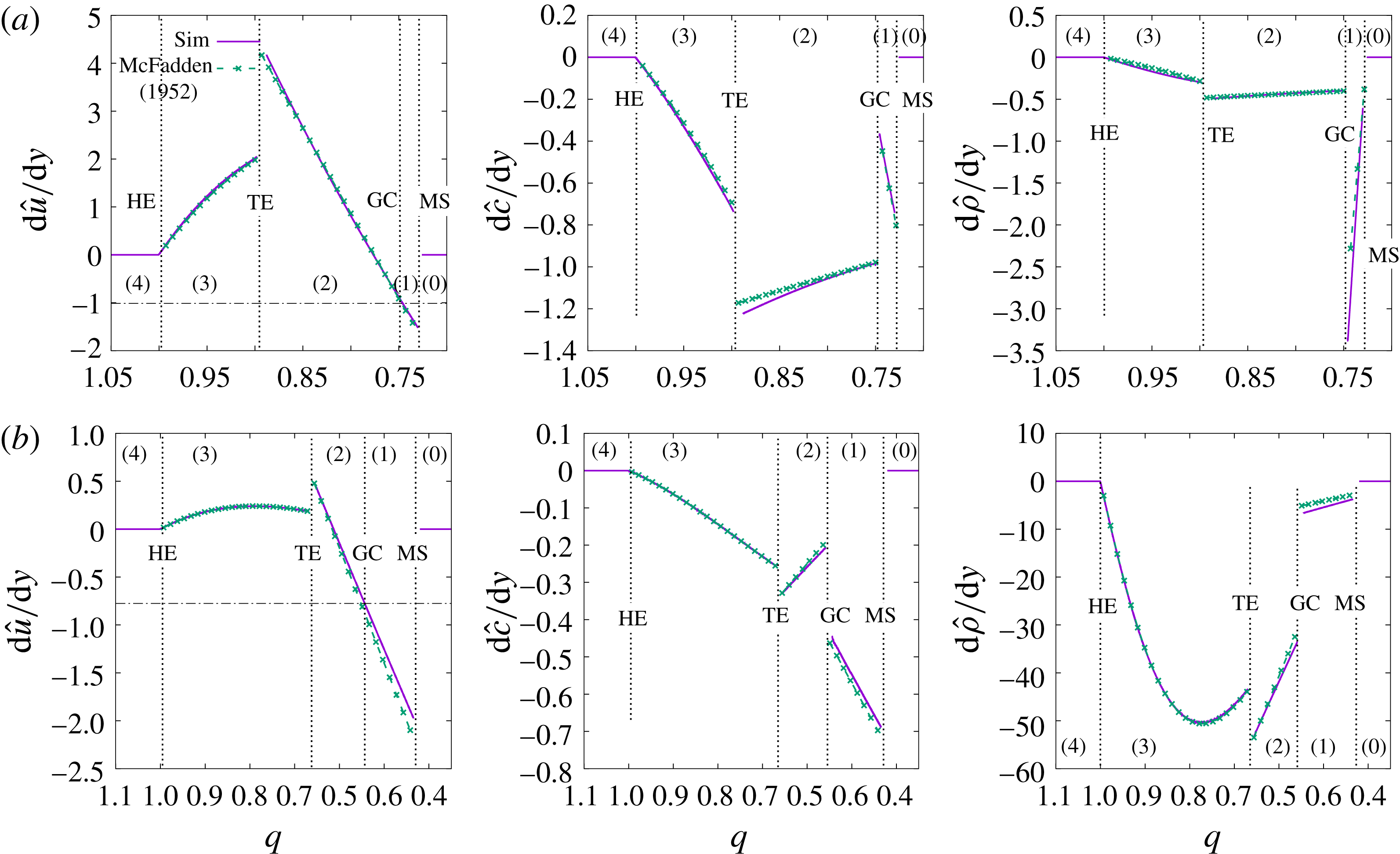
) are shown in figure 7. The results obtained by McFadden’s theory are compared with those obtained numerically and very good agreement is observed. The numerical results for
 $\text{d}\hat{u} /\text{d}y$
,
 $\text{d}{\hat{c}}/\text{d}y$
and
 $\text{d}\hat{\unicode[STIX]{x1D70C}}/\text{d}y$
are calculated based on the difference between the spherical and planar shock-tube results at
 $\hat{t}=0.0067$
.
First-order correction of the spherical blast-wave solution to the planar shock-tube solution for the velocity, the speed of sound and the density for (a) case 1 (
 $p_{4}/p_{0}=121$
,
 $c_{4}/c_{0}=11$
) and (b) case 3 (
 $p_{4}/p_{0}=121$
,
 $c_{4}/c_{0}=1$
) in the asymptotic limit of
 $t=0^{+}$
. The theoretical results of McFadden are compared to the simulation results. MS, GC, TE and HE denote the main shock, the gas contact, the tail and the head of the expansion fan and the regions between these waves are represented by numbers (0)–(4) as defined in figure 1.

The term
 $\text{d}\hat{u} /\text{d}y$
at the gas contact location (
 $\hat{x}=1$
or
 $q=q_{gc}=2/(\unicode[STIX]{x1D6FE}+1)$
) for
 $\unicode[STIX]{x1D6FE}=1.4$
was given by McFadden as
 $$\begin{eqnarray}\frac{\text{d}\hat{u} }{\text{d}y}\bigg|_{q=q_{gc}}=\frac{5}{36}\frac{9M_{ms,pl}^{4}+16M_{ms,pl}^{2}-1}{M_{ms,pl}^{2}(M_{ms,pl}^{2}-1)}\frac{(\text{d}M_{ms}/\text{d}\hat{t})_{t=0^{+}}}{{\hat{c}}_{4}}+\frac{5}{3}\frac{{\hat{c}}_{1,pl}^{2}}{{\hat{c}}_{4}},\end{eqnarray}$$
where
 $(\text{d}M_{ms}/\text{d}t)_{t=0^{+}}$
is the initial deceleration of the main shock. Then the initial deceleration of the gas contact can be obtained as
 $$\begin{eqnarray}\frac{\text{d}\hat{u} _{gc}}{\text{d}\hat{t}}\bigg|_{t=0^{+}}={\hat{c}}_{4}\frac{\text{d}\hat{u} }{\text{d}y}\bigg|_{q=q_{gc}}.\end{eqnarray}$$
The Atwood number at the gas contact can be expanded in a similar manner,
 $$\begin{eqnarray}\mathit{At}_{gc}(y)=\mathit{At}_{gc,pl}+\frac{\text{d}\mathit{At}_{gc}}{\text{d}y}y+O(y^{2}).\end{eqnarray}$$
The coefficient of the first-order term can be computed as
 $$\begin{eqnarray}\frac{\text{d}\mathit{At}_{gc}}{\text{d}y}=\frac{\text{d}\hat{\unicode[STIX]{x1D70C}}_{2}/\text{d}y|_{q=q_{gc}}-\text{d}\hat{\unicode[STIX]{x1D70C}}_{1}/\text{d}y|_{q=q_{gc}}}{\hat{\unicode[STIX]{x1D70C}}_{2,pl}+\hat{\unicode[STIX]{x1D70C}}_{1,pl}}.\end{eqnarray}$$
Since the time derivative of enstrophy is zero at the gas contact (McFadden Reference McFadden1952), i.e.
 $\text{d}{\hat{S}}_{gc}/\text{d}y=0$
, then
 $\text{d}\hat{\unicode[STIX]{x1D70C}}/\text{d}y$
at
 $q=q_{gc}$
can be related to
 $\text{d}c/\text{d}y$
as
 $$\begin{eqnarray}\frac{\text{d}\hat{\unicode[STIX]{x1D70C}}_{gc,2}}{\text{d}y}\bigg|_{q=q_{gc}^{+}}=\frac{5\hat{\unicode[STIX]{x1D70C}}_{2,pl}}{{\hat{c}}_{2,pl}}\frac{\text{d}{\hat{c}}_{gc,2}}{\text{d}y}\bigg|_{q=q_{gc}^{+}},\quad \text{and}\quad \frac{\text{d}\hat{\unicode[STIX]{x1D70C}}_{gc,1}}{\text{d}y}\bigg|_{q=q_{gc}^{-}}=\frac{5\hat{\unicode[STIX]{x1D70C}}_{1,pl}}{{\hat{c}}_{1,pl}}\frac{\text{d}{\hat{c}}_{gc,1}}{\text{d}y}\bigg|_{q=q_{gc}^{-}},\end{eqnarray}$$
for
 $\unicode[STIX]{x1D6FE}=1.4$
. The expressions for
 $\text{d}{\hat{c}}_{2}/\text{d}y$
and
 $\text{d}{\hat{c}}_{1}/\text{d}y$
were given by McFadden (Reference McFadden1952) and thus are not repeated here. The results of
 $\text{d}{\hat{c}}/\text{d}y$
and
 $\text{d}\hat{\unicode[STIX]{x1D70C}}/\text{d}y$
for cases 1 and 3 are shown in figure 7. From the above the initial acceleration of the gas contact Atwood number can be obtained
 $$\begin{eqnarray}\frac{\text{d}\mathit{At}_{gc}}{\text{d}\hat{t}}\bigg|_{t=0^{+}}=\frac{\text{d}\mathit{At}_{gc}}{\text{d}y}{\hat{c}}_{4}.\end{eqnarray}$$
4.1.2 An approximate model for short-term evolution of gas contact
Friedman (Reference Friedman1961) has also investigated the short-term dynamics of the gas contact, but with a different approach from McFadden (Reference McFadden1952). The method of characteristics was used, and the short-term gas contact trajectory was determined from the positive and negative characteristics as illustrated in figure 8. The negative characteristics from region 1 and the positive characteristics from region 2 meet at the gas contact. If both of these families of characteristics are known, then the temporal evolution of the gas contact can be calculated by matching the gas velocity and pressure (as both the gas velocity and pressure are continuous at the gas contact). Since in the short term the main shock follows the shock-area relation of Whitham (Reference Whitham1958), the negative characteristics starting from the main shock at region 1 can be computed. The positive characteristics passing through the expansion fan at region 3 are also known. Because the secondary shock is initially weak, Friedman considered that the positive characteristics do not change slopes when they pass through the secondary shock and thus the characteristics in region 3 can be readily applied to region 2. When the positive and negative characteristics meet at the gas contact, they have to satisfy the continuity of pressure and velocity, which yields the gas contact trajectory in the
 $x$
–
 $t$
diagram. The short-term evolution of the gas contact obtained by Friedman agreed reasonably well with the simulation results of Brode (Reference Brode1955).
Schematic for the simplified model to determine the gas contact trajectory in the short term.

Both the asymptotic expansion approach of McFadden (Reference McFadden1952) and the semi-analytical approach of Friedman (Reference Friedman1961) are somewhat complicated, yet both of them are valid only for a very short time. For the approach of Friedman, since the strength of the secondary shock increases rapidly over time, the approximation that the slope of the positive characteristics remains unchanged while crossing the secondary shock becomes increasingly inaccurate with time (this can be observed in figure 4). When this happens, the gas contact trajectory obtained by Friedman was shown to deviate from the exact results. Here, we propose a simpler model to obtain the initial deceleration of the gas contact by combining the approaches of Friedman and McFadden.
We first approximate the short-term evolution of the main shock with a series expansion
 $$\begin{eqnarray}\hat{x}_{ms}=1+M_{ms,pl}\hat{t}_{ms}+\frac{\unicode[STIX]{x1D6FC}}{2}\hat{t}_{ms}^{2}+O(\hat{t}_{ms}^{3}).\end{eqnarray}$$
The corresponding short-term evolution of the main shock velocity goes as
 $$\begin{eqnarray}\hat{u} _{ms}=M_{ms}=M_{ms,pl}+\unicode[STIX]{x1D6FC}\hat{t}_{ms}+O(\hat{t}_{ms}^{2}).\end{eqnarray}$$
Similar to McFadden (Reference McFadden1952), we only keep the first-order term in the velocity expansion. The coefficient
 $\unicode[STIX]{x1D6FC}$
only depends on the initial values of the high- and low-pressure regions and can be obtained from on the shock-area relation (3.4) as
 $$\begin{eqnarray}\unicode[STIX]{x1D6FC}=-\frac{2M_{ms,pl}}{J(M_{ms,pl})}.\end{eqnarray}$$
So the short-term shock acceleration is given as
 $$\begin{eqnarray}\frac{\text{d}\hat{u} _{ms}}{\text{d}\hat{t}_{ms}}=\frac{\text{d}M_{ms}}{\text{d}\hat{t}_{ms}}=\unicode[STIX]{x1D6FC}=-\frac{2M_{ms,pl}}{J(M_{ms,pl})}+O(\hat{t}_{ms}),\end{eqnarray}$$
which in the limit of
 $M_{ms}\rightarrow \infty$
can be further simplified as
 $\unicode[STIX]{x1D6FC}=-KM_{ms,pl}^{2}$
. Thus, the short-term deceleration of the main shock increases quadratically with shock strength.
As suggested by Friedman (Reference Friedman1961) and also schematically shown in figure 8, we consider that the negative characteristics are straight lines between the main shock and the gas contact. As a result, the points on the main shock trajectory (
 $\hat{x}_{ms},\hat{t}_{ms}$
) can be uniquely mapped to those on the trajectory of the gas contact (
 $\hat{x}_{gc},\hat{t}_{gc}$
) in the
 $x$
–
 $t$
diagram as
 $$\begin{eqnarray}\hat{x}_{gc}=\hat{x}_{ms}+(\hat{u} _{1}-{\hat{c}}_{1})(\hat{t}_{gc}-\hat{t}_{ms}),\end{eqnarray}$$
where
 $\hat{t}_{ms}$
is the time when the characteristic starts from the main shock,
 $\hat{t}_{gc}$
is the time when it reaches the gas contact and the slope of negative characteristic in region 1 is given by
 $\hat{u} _{1}-{\hat{c}}_{1}$
. In the original model of Friedman,
 $\hat{t}_{gc}$
as a function of
 $M_{ms}$
was obtained by matching the velocity and pressure for the negative and positive characteristics that meet at the gas contact. Here we simplify the analysis by assuming
 $\hat{t}_{gc}$
to vary linearly with
 $M_{ms}$
. Namely, we set
 $$\begin{eqnarray}\frac{\text{d}M_{ms}}{\text{d}\hat{t}_{gc}}=\unicode[STIX]{x1D6FD},\end{eqnarray}$$
where
 $\unicode[STIX]{x1D6FD}$
is a coefficient to be determined, which again depends only on the initial condition. Then it can be shown that
 $$\begin{eqnarray}\hat{t}_{gc}=\frac{\unicode[STIX]{x1D6FC}}{\unicode[STIX]{x1D6FD}}\hat{t}_{ms},\end{eqnarray}$$
and by substituting the above expression in (4.20), we get the series expansion of the gas contact trajectory as
 $$\begin{eqnarray}\hat{x}_{gc}=1+\left(M_{ms,pl}\frac{\unicode[STIX]{x1D6FD}}{\unicode[STIX]{x1D6FC}}+(\hat{u} _{1,pl}-{\hat{c}}_{1,pl})\left(1-\frac{\unicode[STIX]{x1D6FD}}{\unicode[STIX]{x1D6FC}}\right)\right)\hat{t}_{gc}+\frac{\unicode[STIX]{x1D6FD}^{2}}{2\unicode[STIX]{x1D6FC}}\hat{t}_{gc}^{2}+O(\hat{t}_{gc}^{3}).\end{eqnarray}$$
The corresponding gas contact velocity is given as
 $$\begin{eqnarray}\hat{u} _{gc}=\left(M_{ms,pl}\frac{\unicode[STIX]{x1D6FD}}{\unicode[STIX]{x1D6FC}}+(\hat{u} _{1,pl}-{\hat{c}}_{1,pl})\left(1-\frac{\unicode[STIX]{x1D6FD}}{\unicode[STIX]{x1D6FC}}\right)\right)+\frac{\unicode[STIX]{x1D6FD}^{2}}{\unicode[STIX]{x1D6FC}}\hat{t}_{gc}+O(\hat{t}_{gc}^{2}).\end{eqnarray}$$
The parameter
 $\unicode[STIX]{x1D6FD}$
can be obtained by matching the initial velocity of the gas contact with the planar shock-tube counterpart, i.e.
 $\hat{u} _{gc}(\hat{t}=0^{+})=\hat{u} _{1,pl}$
and we get
 $$\begin{eqnarray}\unicode[STIX]{x1D6FD}=\frac{\unicode[STIX]{x1D6FC}{\hat{c}}_{1,pl}}{M_{ms,pl}-\hat{u} _{1,pl}+{\hat{c}}_{1,pl}},\end{eqnarray}$$
where
 ${\hat{c}}_{1,pl}$
and
 $\hat{u} _{1,pl}$
are the non-dimensional speed of sound and gas velocity in region 1 as calculated for a planar shock tube. It is known from (4.24) that
 $$\begin{eqnarray}\frac{\text{d}\hat{u} _{gc}}{\text{d}\hat{t}}=\frac{\unicode[STIX]{x1D6FD}^{2}}{\unicode[STIX]{x1D6FC}},\end{eqnarray}$$
then combining (4.18), (4.25) and (4.26), we finally obtain
 $$\begin{eqnarray}\frac{\text{d}\hat{u} _{gc}}{\text{d}\hat{t}}=\,-\left(\frac{{\hat{c}}_{1,pl}}{M_{ms,pl}-\hat{u} _{1,pl}+{\hat{c}}_{1,pl}}\right)^{2}\frac{2M_{ms,pl}}{J(M_{ms,pl})}.\end{eqnarray}$$
The present approximate model yields an explicit prediction of the gas contact deceleration, based on quantities that can be obtained from the planar shock-tube theory and the shock-area relation of Whitham. The present approach does not require a fully asymptotic solution of the Euler equation or a numerical solution of ordinary differential equations (ODE) and thus is easier to use compared to the approaches of McFadden (Reference McFadden1952) and Friedman (Reference Friedman1961).
4.1.3 Comparison with simulation results
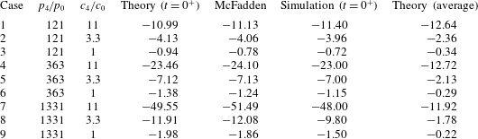
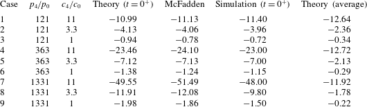
The comparison of the initial deceleration of the gas contact obtained from the present model (4.26), the full asymptotic solution of McFadden (Reference McFadden1952) and the numerical results are summarized in table 4. The difference between the present model and the asymptotic solution of McFadden (Reference McFadden1952) is within 10 % for most cases considered here (except for case 3 where the discrepancy is approximately 18 %). The simulation results generally agree well with the theoretical prediction, including both the present model and that of McFadden (Reference McFadden1952). Except for case 1, the simulations under-predict the magnitude of the deceleration. Considering that initiation of the spherical blast is a singularity in the Euler equations, the discrepancy between the simulation and theoretical results is mainly due to the numerical error near singularity.
It is observed that the magnitude of the gas contact deceleration generally increases with
 $p_{4}/p_{0}$
and
 $c_{4}/c_{0}$
, which is consistent with a previous study by Mankbadi & Balachandar (Reference Mankbadi and Balachandar2012). When
 $p_{4}/p_{0}$
and
 $c_{4}/c_{0}$
increase, the total energy released from the sphere increases correspondingly. As a consequence, the initial strength of the main shock is higher. Since the magnitude of shock deceleration due to the increase of shock area is larger for a stronger shock, see (4.17) (Whitham Reference Whitham1958), the main shock speed decreases faster for stronger shocks. Due to the fact that the deceleration of the gas contact is mainly dictated by that of the main shock (see figure 8), the former follows the same trend as the latter for varying
 $p_{4}/p_{0}$
and
 $c_{4}/c_{0}$
.
Results of the gas contact deceleration
 $\text{d}\hat{u} _{gc}/\text{d}\hat{t}=(\text{d}u_{gc}/\text{d}t)(R_{s}/c_{0}^{2})$
. Columns 4, 5 and 6 are for
 $\text{d}\hat{u} _{gc}/\text{d}\hat{t}$
at
 $t=0^{+}$
; while column 7 is for average
 $\text{d}\hat{u} _{gc}/\text{d}\hat{t}$
up to where the gas contact reaches zero or minimum velocity. The columns 4 and 7 correspond to the present predictions given in (4.26) and (4.29), respectively.
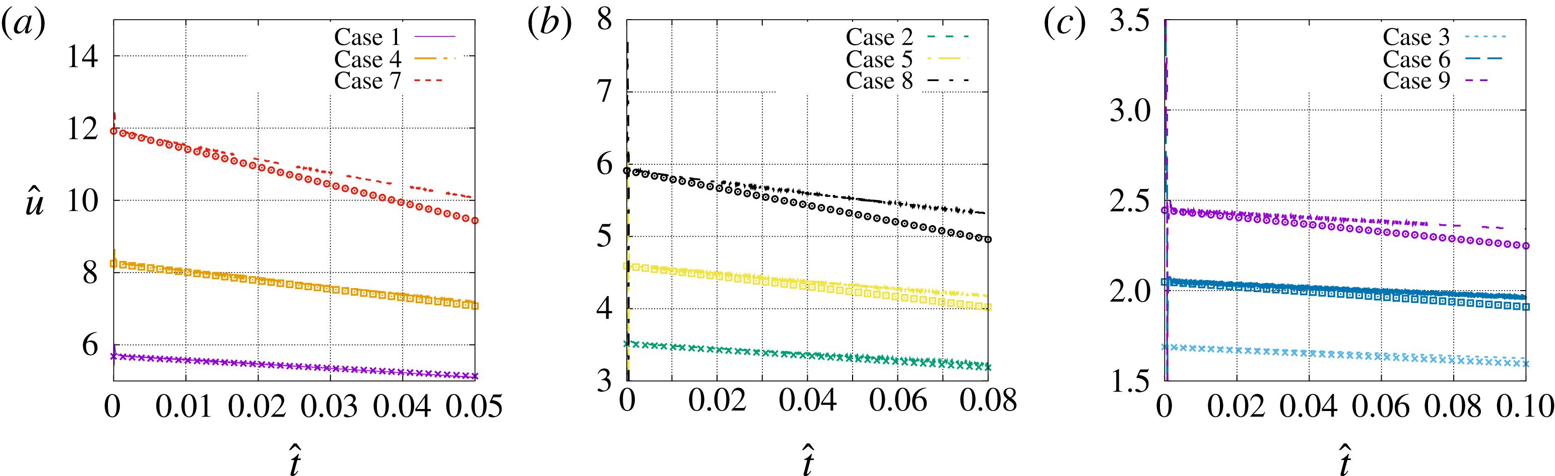
The asymptotic and numerical solutions for the short-term evolution of the gas contact velocity are shown in figure 9. The magnitude of gas contact deceleration decreases in time for all cases. As a result, the asymptotic values given in table 4 are only good estimates for a short period of time, i.e.
 $\hat{t}\lesssim 0.1$
.
Temporal evolution of the gas contact velocity in the short term for (a)
 $c_{4}/c_{0}=11$
, (b)
 $c_{4}/c_{0}=3.3$
and (c)
 $c_{4}/c_{0}=1$
. The symbols and lines represent the asymptotic and numerical solutions, respectively.

If the gas density on the left (in region 2),
 $\unicode[STIX]{x1D70C}_{gc,2}$
, is larger than that on the right (in region 1) of the gas contact,
 $\unicode[STIX]{x1D70C}_{gc,1}$
, namely
 $\mathit{At}_{gc}>0$
, the gas contact discontinuity is unstable based on the RT instability theory. The initial value of
 $\mathit{At}_{gc}$
is identical to that in the planar counterpart (
 $\mathit{At}_{gc,pl}$
), and the variation of which as a function of
 $p_{4}/p_{0}$
and
 $c_{4}/c_{0}$
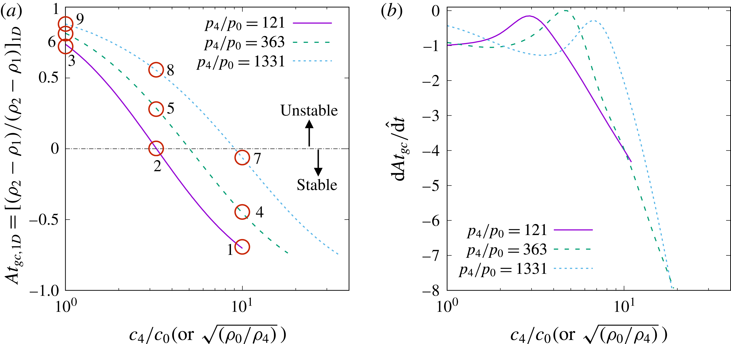
is shown in figure 10(a). In general,
 $\mathit{At}_{gc,pl}$
decreases with
 $c_{4}/c_{0}$
and increases with
 $p_{4}/p_{0}$
. For a given
 $p_{4}/p_{0}$
, there is a critical value of
 $(c_{4}/c_{0})_{crit}$
. For
 $c_{4}/c_{0}$
larger than the critical value,
 $\mathit{At}_{gc,pl}$
becomes negative. For such cases (i.e. cases 1, 4 and 7), the gas contact is initially stable.
(a) Initial value and (b) initial time derivative of the Atwood number at the gas contact, as functions of
 $p_{4}/p_{0}$
and
 $c_{4}/c_{0}$
. Open circles denote cases in table 3.

Temporal evolution of the gas contact velocity: (a) is plotted with
 $\hat{u} =u/c_{0}$
and
 $\hat{t}=tc_{0}/R_{s}$
as the velocity and time scales, while (b–h) are plotted with
 $\tilde{u} =u/c_{4}$
and
 $\tilde{t}=tc_{4}/{\mathcal{L}}$
as the velocity and time scales. For (c–e) the magnitude of
 $u_{gc}$
is plotted in a log–log scale, while for (f–h)
 $u_{gc}$
is plotted in a linear-log scale. The results in (b) are replotted in (c–e) for different
 $c_{4}/c_{0}$
for better visualization.

Temporal evolution of the gas contact radius for different cases (a) with
 $\hat{x}=x/R_{s}$
and
 $\hat{t}=tc_{0}/R_{s}$
as the length and time scales and (b) with
 $\tilde{x}=x/{\mathcal{L}}$
and
 $\tilde{t}=tc_{4}/{\mathcal{L}}$
as the length and time scales.

Finally, the initial time rate of change of the Atwood number at the gas contact, i.e.
 $\text{d}\mathit{At}_{gc}/\text{d}\hat{t}$
, is shown in figure 10(b). It is observed that
 $\text{d}\mathit{At}_{gc}/\text{d}\hat{t}$
is generally negative, so
 $\mathit{At}_{gc}$
will remain negative for
 $\mathit{At}_{gc,pl}<0$
. Therefore, the cases indicated in figure 10(a) as initially stable will remain stable in the short term. For the cases with a positive initial value of
 $\mathit{At}_{gc,pl}$
, as time evolves
 $\mathit{At}_{gc}$
may turn negative. Nevertheless, it can be observed from figure 10 that for the cases with small
 $\mathit{At}_{gc,pl}$
(like case 2), the magnitude of
 $\text{d}\mathit{At}_{gc}/\text{d}\hat{t}$
is also small. Therefore, the early decrease of
 $\mathit{At}_{gc}$
may not change the overall instability of the gas contact.
4.2 Long-term behaviour
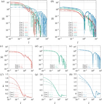
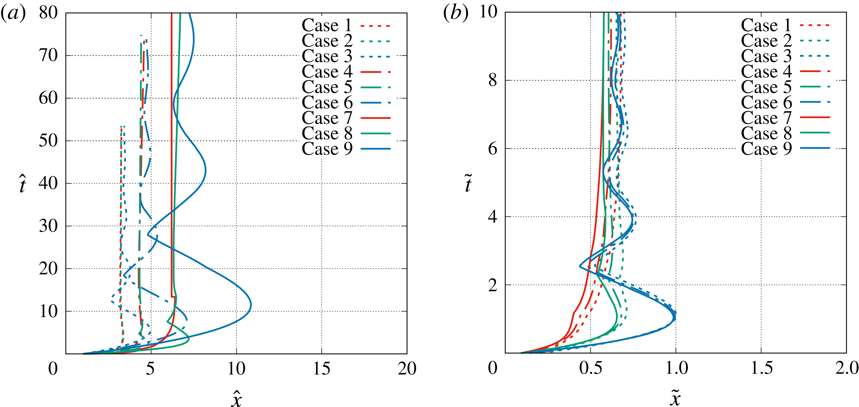
The long-term evolution of the gas contact velocity and location are shown in figures 11(a) and 12(a). As expected, the results for the different initial conditions are far separated when they are not appropriately scaled. In general, the velocity of the gas contact,
 $u_{gc}$
, decreases in time except after the gas contact encounters the secondary and subsequent shocks that reflect from the origin. When the gas contact interacts with these secondary-, tertiary- and higher-order outward propagating shock waves, its outward radial velocity increases. But after each interaction the gas contact starts to decelerate again, until its interaction with the next shock wave. In the three cases (1, 4 and 7) where the sound-speed ratio is 11 the shock–contact interactions occur before the velocity of the gas contact becomes negative. Whereas, in the other cases of lower sound-speed ratios the gas contact velocity becomes negative (i.e. the gas contact starts moving inward) before the interaction with the outward propagating shock, which changes the direction of gas contact motion from inward to outward. This difference can be clearly seen in the linear–log plots shown in figure 11(f–h
) and also manifests as large negative spikes in the log–log plots where the sign of the gas contact velocity changes. The net result is that the gas contact velocity approaches zero in an oscillatory manner. At
 $t\rightarrow \infty$
,
 $u_{gc}\rightarrow 0$
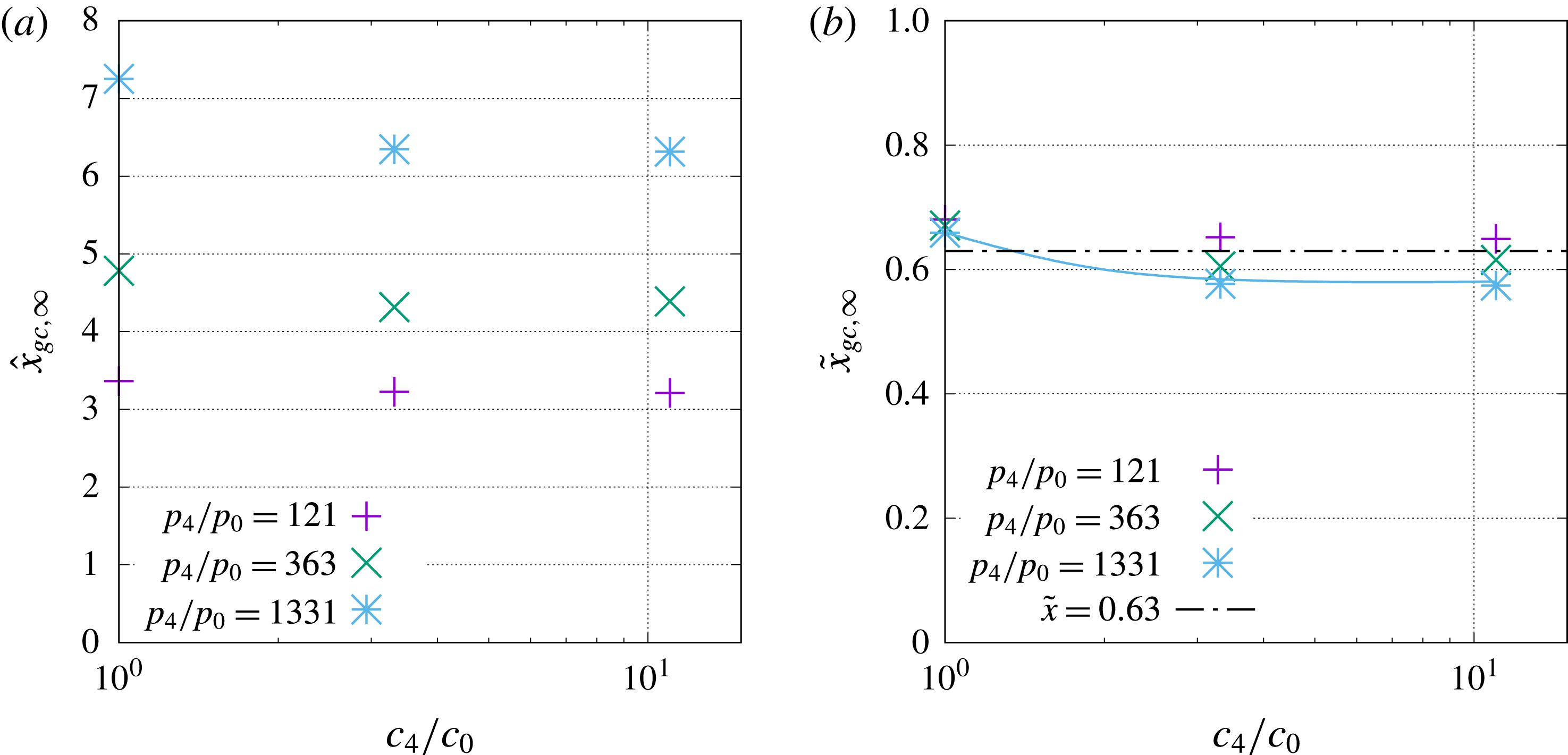
and the gas contact reaches its long-term asymptotic radius
 $x_{gc,\infty }$
.
Since the evolution of the main shock is well characterized by the length scale
 ${\mathcal{L}}$
, it is of interest to examine how well it applies for the gas contact. The temporal evolutions of the location and velocity of the gas contact in terms of dimensionless variables are defined as
 $$\begin{eqnarray}\tilde{x}=\frac{x}{{\mathcal{L}}},\quad \tilde{u} =\frac{u}{c_{4}},\quad \tilde{t}=\frac{tc_{4}}{{\mathcal{L}}},\end{eqnarray}$$
and are shown in figures 11(b–h) and 12(b). Compared to the characteristic velocity of the long-term solution of the main shock, the characteristic velocity chosen for the gas contact is
 $c_{4}$
, which better represents the information propagation speed in the near field (that is made up of the high-pressure gas initially inside the sphere of radius
 $R_{s}$
). It can be observed that the above characteristic scales work well in collapsing the gas contact location and velocity for different initial conditions after the short-term transition period. A close examination of figure 11(c–e) shows that when
 $c_{4}/c_{0}$
is fixed, the gas contact velocities for different
 $p_{4}/p_{0}$
nearly merge together after approximately
 $\tilde{t}=0.3$
. This observation is true for all the three sound-speed ratios considered here, namely
 $c_{4}/c_{0}=11$
, 3.3 and 1.
In particular, it can be seen that the gas contact reaches zero velocity at approximately
 $\tilde{t}\approx 1$
for
 $c_{4}/c_{0}=3.3$
and 1 (see figures 11(d,g) and 11(e,h), respectively). For
 $c_{4}/c_{0}=11$
, the gas contact is overtaken by the secondary shock, resulting in a rise of the gas contact velocity, so the gas contact reaches a local minimum value which is small but remains positive. This self-similar behaviour enables to us to obtain an estimate of the average deceleration of the gas contact for an intermediate time
 $\tilde{t}\lesssim 1$
(i.e. before interaction with the secondary shock) as
 $$\begin{eqnarray}\frac{\text{d}\tilde{u} _{gc}}{\text{d}\tilde{t}}\bigg|_{ave}=\tilde{u} _{gc,pl},\quad \text{or}\quad \frac{\text{d}u_{gc}}{\text{d}t}\bigg|_{ave}=\frac{u_{gc,pl}\,c_{4}}{{\mathcal{L}}}.\end{eqnarray}$$
Previous works have shown that for an intermediate time the deceleration and Atwood number of the gas contact are nearly time invariant (Mankbadi & Balachandar Reference Mankbadi and Balachandar2012), and as a result small perturbations of the gas contact grow exponentially following classical RT instability. Here, equation (4.29) provides an approximate estimate for the average deceleration of the gas contact in this intermediate time regime and the values for different cases are shown in table 4. Different from the initial deceleration of the gas contact, which increases significantly with
 $p_{4}/p_{0}$
, the average deceleration decreases only slightly with
 $p_{4}/p_{0}$
for the same
 $c_{4}/c_{0}$
. As a result, the average deceleration of the gas contact is mainly dictated by
 $c_{4}/c_{0}$
, and it is seen that
 $\text{d}u_{gc}/\text{d}t|_{ave}$
decreases with
 $c_{4}/c_{0}$
. Furthermore, it is also observed that the difference between the initial and average deceleration magnifies with
 $p_{4}/p_{0}$
.
Similar long-term self-similar behaviour is also observed in the temporal evolution of the gas contact radius in figure 12. In figure 12(a), the dimensionless variables
 $\hat{x}=x/R_{s}$
and
 $\hat{t}=tc_{0}/R_{s}$
are used and, as can be seen, the gas contact trajectories for different cases are all very different; while in figure 12(b), where we used
 $\tilde{x}=x/{\mathcal{L}}$
and
 $\tilde{t}=tc_{4}/{\mathcal{L}}$
, it is observed that the results for different
 $p_{4}/p_{0}$
and the same
 $c_{4}/c_{0}$
collapse. The difference between the two figures is not only due to the scaling of the different sound speeds but also the different length scales.
For the main shock there exists a general approximate similarity solution that is independent of both
 $p_{4}/p_{0}$
and
 $c_{4}/c_{0}$
; while for the gas contact we only observe a semi-similarity solution which does not depend on
 $p_{4}/p_{0}$
but varies with
 $c_{4}/c_{0}$
. Since the gas contact at all times remains in the near field, its motion is highly related to the speed of the secondary shock, which in turn is dictated by the sound speed in the pressurized gas. When
 $c_{4}/c_{0}$
varies, the pattern of interaction between the secondary shock and the gas contact changes significantly, as shown in figure 2.
As a result, the semi-similar solution for the gas contact can be written, similar to (3.18) and (3.19), as
 $$\begin{eqnarray}\displaystyle & \displaystyle \tilde{x}_{gc}=\unicode[STIX]{x1D701}_{sim}\left(\tilde{t},\frac{c_{4}}{c_{0}}\right), & \displaystyle\end{eqnarray}$$
 $$\begin{eqnarray}\displaystyle & \displaystyle \tilde{u} _{gc}=\unicode[STIX]{x1D701}_{sim}^{\prime }\left(\tilde{t},\frac{c_{4}}{c_{0}}\right)\quad \text{for }\tilde{t}\,\gtrsim \,\tilde{t}_{sim}. & \displaystyle\end{eqnarray}$$
The semi-similarity function
 $\unicode[STIX]{x1D701}_{sim}^{\prime }$
(or
 $\unicode[STIX]{x1D701}_{sim}$
) varies with
 $c_{4}/c_{0}$
as shown in figures 11(c–h) and 12(b).
4.3 Asymptotic radius of the gas contact at infinite time
Although the path of the gas contact towards its asymptotic radius
 $\tilde{x}_{gc,\infty }$
varies with
 $c_{4}/c_{0}$
(see figure 12), the value of
 $\tilde{x}_{gc,\infty }$
itself varies little with
 $c_{4}/c_{0}$
. Here we take the gas contact radius at
 $\tilde{t}=10$
as an approximation of
 $\tilde{x}_{gc,\infty }$
and the results for the different cases are shown in figure 13. If the asymptotic contact radius is normalized by
 $R_{s}$
,
 $\hat{x}_{gc,\infty }$
varies over a wide range for the different cases considered in this study, from approximately 3.2 to approximately 7.2. Instead, if we use the length scale
 ${\mathcal{L}}$
, it is shown in figure 13(b) that
 $\tilde{x}_{gc,\infty }=x_{gc,\infty }/{\mathcal{L}}$
for different
 $p_{4}/p_{0}$
collapse. It is observed that
 $\tilde{x}_{gc,\infty }$
decreases slightly with
 $c_{4}/c_{0}$
. For large
 $c_{4}/c_{0}$
 $\tilde{x}_{gc,\infty }$
becomes a constant.
In general
 $\tilde{x}_{gc,\infty }$
varies little with either
 $p_{4}/p_{0}$
or
 $c_{4}/c_{0}$
and is almost a constant for all cases considered here. The average value of
 $\tilde{x}_{gc,\infty }$
for all the nine cases is approximately 0.63 with a standard deviation of 0.04. The approximate asymptotic radius of the gas contact can thus be expressed as
 $$\begin{eqnarray}\tilde{x}_{gc,\infty }\approx 0.63\quad \text{or}\quad x_{gc,\infty }\approx 0.63R_{s}(p_{4}/p_{0})^{1/3}.\end{eqnarray}$$
Asymptotic radius of the gas contact. More cases are run for
 $p_{4}/p_{0}=1331$
to obtain the blue curve.

It is interesting to observe that the length scale
 ${\mathcal{L}}=R_{s}(p_{4}/p_{0})^{1/3}$
, which well characterizes the far-field feature of the main shock, also performs remarkably well for the asymptotic long-term evolution of the gas contact. It should be noted that the scaling
 $(p_{4}/p_{0})^{1/3}$
in the length scale
 ${\mathcal{L}}$
was dictated by the total energy initially contained in the pressurized gas sphere. As the main shock propagates much farther than the initial charge radius
 $R_{s}$
, it is reasonable to neglect the finite-size effect of the spherical energy source and to treat the finite source as a point source. Thus, the long-term evolution of the main shock in the far field is expected to be well characterized by
 ${\mathcal{L}}$
and follow the scaling
 $(p_{4}/p_{0})^{1/3}$
. However, this point-source argument for the main shock in the far field is not applicable to the gas contact since the latter stays in the near field all the time. In order to explain the observed scaling law for the asymptotic radius of the gas contact, a simple model is considered here following the previous study of bubble oscillation (Aref & Balachandar Reference Aref and Balachandar2017).
In this simple model, we ignore the compressibility effect (which is only appropriate for
 $\tilde{t}\gg 1$
when the compressibility effect becomes weak) so the flow outside the gas contact satisfies the continuity condition,
 $$\begin{eqnarray}ux^{2}=u_{gc}x_{gc}^{2}.\end{eqnarray}$$
Substituting the above into the momentum equation, equation (2.2), the latter becomes
 $$\begin{eqnarray}\frac{x_{gc}^{2}}{x^{2}}\frac{\text{d}^{2}x_{gc}}{\text{d}t^{2}}+\frac{2x_{gc}}{x^{2}}\left(\frac{\text{d}x_{gc}}{\text{d}t}\right)^{2}-\frac{2x_{gc}^{4}}{x^{5}}\frac{\text{d}x_{gc}}{\text{d}t}=-\frac{1}{\unicode[STIX]{x1D70C}_{0}}\frac{\unicode[STIX]{x2202}p}{\unicode[STIX]{x2202}x}.\end{eqnarray}$$
It is further assumed that the gas pressure inside the gas contact is uniform and follows a polytropic law as
 $$\begin{eqnarray}p(x_{gc})^{3\unicode[STIX]{x1D702}}=p_{4}(R_{s})^{3\unicode[STIX]{x1D702}},\end{eqnarray}$$
where
 $\unicode[STIX]{x1D702}=1$
and
 $\unicode[STIX]{x1D6FE}$
for isothermal and isentropic processes, respectively. Then (4.34) can be integrated from
 $x_{gc}$
to infinity to yield
 $$\begin{eqnarray}x_{gc}\frac{\text{d}^{2}x_{gc}}{\text{d}t^{2}}+\frac{3}{2}\left(\frac{\text{d}x_{gc}}{\text{d}t}\right)^{2}=-\frac{p_{0}-p_{4}(R_{s}/x_{gc})^{3\unicode[STIX]{x1D702}}}{\unicode[STIX]{x1D70C}_{0}}.\end{eqnarray}$$
The above equation governing the gas contact evolution is similar to the well-known Rayleigh equation for the dynamics of bubbles.
If we introduce a dimensionless variable
 $\unicode[STIX]{x1D712}=(x_{gc}/R_{s})^{5/2}$
, the above equation can be rewritten as
 $$\begin{eqnarray}\frac{\text{d}^{2}\unicode[STIX]{x1D712}}{\text{d}t^{2}}=\frac{5}{2}\frac{(p_{4}/p_{0})\unicode[STIX]{x1D712}^{-6\unicode[STIX]{x1D702}/5}-1}{p_{4}/p_{0}-1}\unicode[STIX]{x1D712}^{1/5}.\end{eqnarray}$$
When the gas contact reaches the asymptotic radius,
 $\text{d}^{2}\unicode[STIX]{x1D712}/\text{d}t^{2}=0$
. Then the numerator of the right-hand side has to be equal to zero, so we can obtain
 $$\begin{eqnarray}\unicode[STIX]{x1D712}_{\infty }=\left(\frac{x_{gc,\infty }}{R_{s}}\right)^{5/2}=\left(\frac{p_{4}}{p_{0}}\right)^{5/6\unicode[STIX]{x1D702}}\end{eqnarray}$$
or
 $$\begin{eqnarray}\frac{x_{gc,\infty }}{R_{s}}=\left(\frac{p_{4}}{p_{0}}\right)^{1/3\unicode[STIX]{x1D702}}.\end{eqnarray}$$
The asymptotic contact radius obtained from the model depends only on the initial pressure ratio
 $p_{4}/p_{0}$
. When
 $\unicode[STIX]{x1D702}=1$
, we recover the scaling law shown in (4.32) and the constant coefficient
 $0.63$
can be taken to account for all the approximations made in the above simple analysis.
5 Secondary shock wave
5.1 Short-term behaviour
The secondary shock forms at the tail of the expansion fan. The secondary shock is initially a weak compression wave, and its strength increases in time. The secondary shock initially moves outward and eventually reverses direction and moves inward.
The initial dynamics of the compression wave at the tail of the expansion fan (which has not yet become a shock) can be solved, following the asymptotic approach of McFadden (Reference McFadden1952). It is shown in figure 7 that initially
 $\text{d}u_{te}/\text{d}t=\text{d}^{2}x_{te}/\text{d}t^{2}>0$
. In other words, the tail of the expansion fan indeed accelerates initially and its trajectory bends outward as shown in figure 14 (see in particular cases 1, 2 and 4), and also shown schematically in figure 8. Nevertheless, the acceleration of the secondary shock decreases very fast and the secondary shock soon starts to decelerate. The acceleration of the secondary shock lasts for such a short time that it is sometimes not easy to observe.
The motion of the secondary shock at small but finite time can be approximately captured by the weak-shock approximation of Chisnell (Reference Chisnell1957), as discussed by Friedman (Reference Friedman1961). The shock speed is equal to the average of the slopes of the incoming characteristics at a given location in the
 $x$
–
 $t$
diagram (see figure 4). The initial evolution of the secondary shock wave was approximately solved by Friedman (Reference Friedman1961) semi-analytically. The negative characteristics from the main shock are needed. The characteristics will change when they pass through the gas contact, so the gas contact evolution need to be known a priori. As explained in the previous section, the gas contact motion can only be solved analytically when the secondary shock is considered as weak and its impact on the positive characteristics passing through is negligible. When the secondary shock strengthens, the dynamics of the secondary shock and the gas contact are coupled. Furthermore, when the secondary shock strengthens, the weak-shock approximation of Chisnell is no longer valid. Therefore, the approach of Friedman (Reference Friedman1961) remains a good approximate only for a short time. A numerical solution is in general required to calculate the evolution of the secondary shock.
5.2 Long-term behaviour
The temporal evolution of the secondary shock wave is shown in figure 14. Similar to the main shock and the gas contact, we examine the performance of the length scale
 ${\mathcal{L}}$
in characterizing the long-term evolution of the secondary shock. The secondary shock radius, if normalized by
 $R_{s}$
, is observed to be quite different from case to case. Instead if we use the length scale
 ${\mathcal{L}}$
, it is seen that the trajectories of the secondary shock (
 $\tilde{x}_{2s}=x_{2s}/{\mathcal{L}}$
) for the different pressure ratios
 $p_{4}/p_{0}$
approximately collapse, provided that the sound-speed ratio
 $c_{4}/c_{0}$
remains the same.
Temporal evolution of the secondary shock wave for different initial conditions, (a) with
 $\hat{x}=x/R_{s}$
and
 $\hat{t}=tc_{0}/R_{s}$
as the length and time scales and (b) with
 $\tilde{x}=x/{\mathcal{L}}$
and
 $\tilde{t}=tc_{4}/{\mathcal{L}}$
as the length and time scales.

Similar to (4.30) and (4.31), a semi-similar solution for the secondary shock can be expressed as
 $$\begin{eqnarray}\displaystyle & \displaystyle \tilde{x}_{2s}=\unicode[STIX]{x1D719}_{sim}\left(\tilde{t},\frac{c_{4}}{c_{0}}\right), & \displaystyle\end{eqnarray}$$
 $$\begin{eqnarray}\displaystyle & \displaystyle \tilde{u} _{2s}=\unicode[STIX]{x1D719}_{sim}^{\prime }\left(\tilde{t},\frac{c_{4}}{c_{0}}\right)\quad \text{for }\tilde{t}\,\gtrsim \,\tilde{t}_{sim}. & \displaystyle\end{eqnarray}$$
Again, the self-similar solutions
 $\unicode[STIX]{x1D719}$
and
 $\unicode[STIX]{x1D719}^{\prime }$
depend on the sound-speed ratio
 $c_{4}/c_{0}$
and can be obtained numerically.
Scaling results of the secondary shock wave. (a) The maximum radius the secondary shock reaches (
 $x_{2s,max}$
); (b) the time when the secondary shock reaches the origin (
 $t_{2s,x=0}$
); (c) the time when the secondary shock overtakes the gas contact (
 $t_{2s,gc}$
).

The long-term temporal evolution of the secondary shock can be characterized by the following quantities as indicated in figure 2(b):
(i)
$x_{2s,max}$
: the maximum radius the secondary shock reaches when it first reverses direction;(ii)
$t_{2s,x=0}$
: the time for the secondary shock to converge to the origin;(iii)
$t_{2s,gc}$
: the time for the reflected secondary shock to interact with the gas contact.


They are shown as functions of
 $p_{4}/p_{0}$
and
 $c_{4}/c_{0}$
in figure 15(a–c
), respectively. It is observed that these quantities in the conventional dimensionless form, namely
 $\hat{x}$
and
 $\hat{t}$
, vary with both
 $p_{4}/p_{0}$
and
 $c_{4}/c_{0}$
, see the first row of figure 15. Nevertheless, when the long-term length and time scales
 ${\mathcal{L}}$
and
 ${\mathcal{L}}/c_{4}$
are used to scale the results, then
 $\tilde{x}_{2s,max}$
,
 $\tilde{t}_{2s,x=0}$
and
 $\tilde{t}_{2s,gc}$
are all independent of
 $p_{4}/p_{0}$
. The variations of
 $\tilde{x}_{2s,max}$
,
 $\tilde{t}_{2s,x=0}$
and
 $\tilde{t}_{2s,gc}$
with
 $c_{4}/c_{0}$
are indicated by the blue curves in figure 15. More cases for different
 $c_{4}/c_{0}$
were run to generate a smooth curve for
 $p_{4}/p_{0}=1331$
.
When the secondary shock overtakes the gas contact, the RM instability will be triggered. From figure 15(c), it can be observed that the shock–contact interaction time for different pressure ratios collapse when scaled by the proposed time scale
 ${\mathcal{L}}/c_{4}$
. Therefore, the current scaling relation is useful to predict the initiation time (and radius) of the RM instability.
The initial growth of RM instability depends on the shock Mach number (
 $M_{2s,gc}$
) and the Atwood number of the gas contact (
 $\mathit{At}_{gc,2s}$
) at the time of shock–contact interaction (Brouillette Reference Brouillette2002). The values of
 $M_{2s,gc}$
and
 $\mathit{At}_{gc,2s}$
for the present cases are shown in table 5. It is seen that for a fixed
 $p_{4}/p_{0}$
, that
 $M_{2s,gc}$
and
 $\mathit{At}_{gc,2s}$
generally increase when
 $c_{4}/c_{0}$
decreases. For the same
 $c_{4}/c_{0}$
,
 $M_{2s,gc}$
increases only slightly with
 $p_{4}/p_{0}$
; while
 $\mathit{At}_{gc,2s}$
increases much faster with
 $p_{4}/p_{0}$
. Different from the RT instability, the RM instability will grow no matter whether the density gradient is positive or negative, so the absolute value of
 $\mathit{At}_{gc,2s}$
is of importance.
The Mach number of the secondary shock and the Atwood number of the gas contact when the secondary shock overtakes the gas contact.
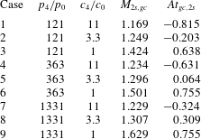
6 Conclusions
A spherical blast generated by suddenly releasing a sphere of compressed gas is investigated in the present study. The resulting spherical blast wave can be characterized by the evolution of the main shock wave, the gas contact discontinuity, the secondary shock wave and the interactions between these waves. The gas flow is mainly dictated by the initial condition, namely the initial pressure and sound-speed ratios between the compressed gas and the ambiance:
 $p_{4}/p_{0}$
and
 $c_{4}/c_{0}$
. Numerical simulations are performed for a wide range of
 $p_{4}/p_{0}$
and
 $c_{4}/c_{0}$
and the simulation results are used to establish scaling laws and self-similar solutions.
6.1 Conclusions on the main shock
While the main shock trajectory varies significantly with the initial condition, an approximate similarity solution exists for the long-term evolution of the main shock,
 $tc_{4}/R_{s}\gg 1$
. A long-term length scale
 ${\mathcal{L}}$
is proposed, which is shown to approximately collapse the computed shock trajectories for a wide range of
 $p_{4}/p_{0}$
and
 $c_{4}/c_{0}$
. The length scale
 ${\mathcal{L}}$
incorporates the sphere radius (
 $R_{s}$
) and the initial pressure ratio (
 $p_{4}/p_{0}$
), i.e.
 ${\mathcal{L}}=R_{s}(p_{4}/p_{0})^{1/3}$
. When the main shock is strong, this similarity solution is consistent with the Taylor–Sedov blast-wave theory and the speed of the main shock follows the scaling
 $u_{ms}\sim t^{-3/5}$
. When the main shock becomes weak, the shock speed is observed to obey a different scaling, i.e.
 $(u_{ms}-1)\sim t^{-1}$
. It is further observed that the short-term (
 $tc_{4}/R_{s}\ll 1$
) evolution of the main shock follows the shock-area relation. Combining the short-term shock-area relation and the long-term self-similarity solution, the evolution of the main shock over the entire time span has been obtained semi-analytically.
6.2 Conclusions on the gas contact
Due to the radial effect, the gas contact decelerates as it propagates outward. If the radial gradient of density is negative, then Rayleigh–Taylor (RT) instability will be triggered. In the present study the short-term deceleration and Atwood number of the contact are obtained analytically using the method of characteristics and asymptotic analysis.
Due to repeated interactions with the reflected secondary and subsequent shocks, the velocity of the gas contact decreases and approaches zero in an oscillatory manner. When
 ${\mathcal{L}}$
and the speed of sound of the initial high-pressure gas
 $c_{4}$
are used as the length and velocity scales, the long-term evolution of the gas contact for different
 $p_{4}/p_{0}$
approximately collapses. It is observed that the gas contact velocity for all the cases decreases to zero for the first time during its oscillatory evolution at approximately
 $t={\mathcal{L}}/c_{4}$
.
Different from the main shock, only a semi-similar solution exists for the gas contact, i.e. the similarity functions for gas contact radius and velocity do not depend on
 $p_{4}/p_{0}$
, but will vary with
 $c_{4}/c_{0}$
. Although the rate of change for the gas contact to reach its asymptotic terminal radius (
 $x_{gc,\infty }$
) varies with
 $c_{4}/c_{0}$
, the value of
 $x_{gc,\infty }$
depends mainly on
 $p_{4}/p_{0}$
and from the simulation results it is observed that
 $x_{gc,\infty }\approx 0.63R_{s}(p_{4}/p_{0})^{1/3}$
. A simple theoretical model is developed to explain this scaling relation.
6.3 Conclusions on the secondary shock
The radial effect on the short-term evolution of the secondary shock has been evaluated using an asymptotic analysis. It is shown that the secondary shock initially accelerates, but as time evolves the secondary shock soon starts to decelerate. The long-term evolution of the secondary shock is found to be well characterized by the length scale
 ${\mathcal{L}}$
and exhibits a semi-similar solution which depends on
 $c_{4}/c_{0}$
, similar to the gas contact. When the reflected secondary shock interacts with the gas contact, the resulting Richtmyer–Meshkov instability depends on the shock strength. Due to the semi-similar behaviour of both the gas contact and the secondary shock, the dimensionless time for the secondary shock to overtake the gas contact is observed to be independent of
 $p_{4}/p_{0}$
and varies only with
 $c_{4}/c_{0}$
.
Acknowledgements
The financial support of the Department of Mechanical Engineering at Baylor University for this project is gratefully acknowledged. This work was also supported by the US Department of Energy, National Nuclear Security Administration, Advanced Simulation and Computing Program, as a Cooperative Agreement under the Predictive Science Academic Alliance Program, under Contract no. DE-NA0002378. S.B. was also supported in part by the Defense Threat Reduction Agency, Basic Research Award no. HDTRA1-14-1-0028 to University of Florida. The authors would also acknowledge the support from the High Performance and Research Computing Services at Baylor University.