1 Introduction
The process of fragmentation of a bulk liquid mass into fine droplets is known as atomization. This topological transformation of liquid mass is either caused by the inherent instabilities associated with a liquid jet/sheet or realized by specific means to augment the destabilizing effects (Lefebvre & McDonell Reference Lefebvre and McDonell2017). One such method is atomization by jet impact. The most commonly used configuration of oblique impingement of two liquid jets, which is also known as impinging jet atomization, is often employed in liquid propellant rocket engines (Heidmann, Priem & Humphrey Reference Heidmann, Priem and Humphrey1957). The impingement of two coplanar liquid jets of the same momentum produces a leaf-like liquid sheet in a plane perpendicular to the plane of the jets (Taylor Reference Taylor1961). The liquid sheet expands radially from the impingement point while simultaneously thinning and ultimately breaking into drops (Bremond & Villermaux Reference Bremond and Villermaux2006).
The fundamental aspects of liquid sheet breakup in the context of the colliding jets configuration have been studied extensively so far, thereby developing understanding about the dominant mechanisms responsible for drop formation. Heidmann et al. (Reference Heidmann, Priem and Humphrey1957) observed that the sheet undergoes transition from a smooth to a fully developed regime through a stage of periodic breakup depending upon the operating conditions. Bush & Hasha (Reference Bush and Hasha2004) further detailed the transition pattern as oscillating streams, a sheet having a disintegrating rim, fluid chains, fishbones, spluttering chains, a disintegrating sheet and a violently flapping sheet. Attempts were also made to study the breakup of an axisymmetric liquid sheet essentially to capture the flow physics by reducing the complexity of the phenomenon to only the radial dimension (Huang Reference Huang1970; Clanet & Villermaux Reference Clanet and Villermaux2002; Villermaux & Clanet Reference Villermaux and Clanet2002). However, oblique jet impingement produces a leaf-like sheet in which the sheet thickness depends on the azimuthal coordinate also (Taylor Reference Taylor1961; Choo & Kang Reference Choo and Kang2002). Loss of axisymmetry significantly affects the breakup of the sheet in various regions with respect to the impingement point (Bremond & Villermaux Reference Bremond and Villermaux2006).
There are in general two major classes of instabilities that cause distinctive breakup of a liquid sheet under various operating conditions, like the jet velocity (Li & Ashgriz Reference Li and Ashgriz2006). At low jet velocities, the sheet is bounded by a thicker rim that collects the liquid coming through the sheet. The cylindrical rim breaks due to the capillary instability of Rayleigh–Plateau type (Rayleigh Reference Rayleigh1879; Bush & Hasha Reference Bush and Hasha2004). It was also argued that this breakup is also influenced by a centrifugal Raleigh–Taylor instability (Bush & Hasha Reference Bush and Hasha2004) due to the curvature of the rim. When the sheet velocity increases and becomes large enough with respect to the ambient gas, the sheet starts to behave like a flapping flag (Bush & Hasha Reference Bush and Hasha2004; Jung et al. Reference Jung, Hoath, Martin and Hutchings2010). This leads to sheet breakup by the shear instability of Kelvin–Helmholtz type (Lin Reference Lin2003; Li & Ashgriz Reference Li and Ashgriz2006), wherein the amplified waves reaching the bottom part of the sheet disrupt the sheet. However, the rim of the sheet still breaks up in a similar fashion as mentioned previously. This combined breakup often leads to segregated drop sizes, coarse drops being shed from the rim and fine drops from the wavy breakup of the sheet (Villermaux & Clanet Reference Villermaux and Clanet2002). Recent study also shows that it is the thinning effect of the sheet rather than the shear instability that describes the breakup of the flapping sheet better (Majumdar & Tirumkudulu Reference Majumdar and Tirumkudulu2018). The problem of liquid sheet breakup has also been tackled by many researchers using the linearized stability theory and good agreement has been found with experimental observations. A detailed review of this tool may be found in the book of Lin (Reference Lin2003).
The breakup of planar liquid sheets under the influence of external perturbations, either mechanical or acoustic, has been studied from applied as well as fundamental points of view. Crapper, Dombrowski & Pyott (Reference Crapper, Dombrowski and Pyott1975) reported flag-like flapping of a thin liquid sheet generated from a mechanically vibrated injector. Rhys (Reference Rhys1999) studied the influence of acoustics on the stability of a flat liquid sheet produced from a rectangular orifice. It was observed that, at a fixed decibel level, the sheet response was significant at lower frequencies. Also, at a fixed frequency, the amplitude of the sheet undulation/flapping increased with the sound intensity. Bremond, Clanet & Villermaux (Reference Bremond, Clanet and Villermaux2007) conducted experiments with the head-on collision of a liquid jet on a cylindrical rod that is oscillated axially to induce perturbations at the impact point in a controlled manner. The undulating circular sheet, thus formed, undergoes a secondary instability termed a wavy corridor that is responsible for ligament and drop ejection from preferential sites on the sheet edge.
Experiments on head-on jet impingement show that the sheet responds to the acoustic forcing at a certain minimum sound pressure level, and this minimum sound pressure level increases with increase in the excitation frequency (Mulmule, Tirumkudulu & Ramamurthi Reference Mulmule, Tirumkudulu and Ramamurthi2010). The sheet diameter and the drop size were also found to decrease in the presence of acoustic excitation (Mulmule et al. Reference Mulmule, Tirumkudulu and Ramamurthi2010). Similar observations were reported in the case of leaf-like sheets of water by Dighe & Gadgil (Reference Dighe and Gadgil2018). It was also shown that the droplet shedding frequency matches with the excitation frequency when the excitation frequency is below the natural droplet shedding frequency (Dighe & Gadgil Reference Dighe and Gadgil2018). In both studies, the water sheets are seen to respond at certain intermediate frequencies that are not integer multiples of each other, and hence the possibility of resonance was ruled out. However, the reason for this is not clearly understood. The stability of radially moving circular liquid sheets when only the impingement point is perturbed by the acoustics was assessed by Paramati, Tirumkudulu & Schmid (Reference Paramati, Tirumkudulu and Schmid2015). The existence of a critical Weber number was reported, below which the sheet thinning effect dominates the breakup irrespective of the excitation frequency. Further, Majumdar & Tirumkudulu (Reference Majumdar and Tirumkudulu2016) compared the growth rates predicted by the inviscid theory of Tirumkudulu & Paramati (Reference Tirumkudulu and Paramati2013), which takes into account the thinning effect, the surface tension and the inertia of the sheet, but ignores the surrounding gas interaction, with the measurements of Crapper et al. (Reference Crapper, Dombrowski and Pyott1975) and found good agreement.
Atomization from a liquid sheet formed by jet impact is a critical process particularly in the context of its application in liquid rocket engines. The high-energy-density combustors of liquid rocket engines are known to have a varying pressure field as a consequence of unsteady combustion phenomena. The acoustic field in the combustors may affect the process of atomization and form a closed-loop feedback cycle triggering the combustion instability. It has been noted that the impinging jet atomization forms a self-excited system (Bremond & Villermaux Reference Bremond and Villermaux2006) and is prone to sustain the combustion instability (Heidmann et al. Reference Heidmann, Priem and Humphrey1957; Oefelein & Yang Reference Oefelein and Yang1993; Anderson & Yang Reference Anderson and Yang1995; Anderson et al. Reference Anderson, Miller, Ryan, Pal, Santoro and Dressler1998). Moreover, there are certain flow conditions when the impinging jets show periodic atomization (Bush & Hasha Reference Bush and Hasha2004) that may couple with the acoustic field. In view of this, the effect of the acoustic field on the liquid sheet breakup needs attention. It will provide important insights into the behaviour of sheet instabilities triggered by infinitesimal perturbations in the pressure field.
In this paper, we address the influence of external acoustic waves on the breakup processes in a smooth laminar liquid sheet formed by the oblique impingement of two liquid jets. Although the existence of discrete frequencies affecting the sheet breakup has been reported for water sheets (Mulmule et al. Reference Mulmule, Tirumkudulu and Ramamurthi2010; Dighe & Gadgil Reference Dighe and Gadgil2018), Bremond et al. (Reference Bremond, Clanet and Villermaux2007) observed a clear transition between the stable and the unstable forcing frequencies for mechanical perturbations. The effect of acoustic excitation on the breakup of a smooth laminar liquid sheet is assessed in the context of the above contrasting observations. The details of the experimental set-up and the visualization methodologies are provided in § 2. Section 3 describes the experimental observations related to the effect of acoustic parameters on the sheet breakup and the sheet characteristics. Existing theoretical formulations are used in § 4 to predict the stability characteristics in the presence of acoustic forcing and compared with the experimental results. Section 5 gives the concluding remarks, followed by an appendix to discuss the effect of acoustic forcing on very-low-Weber-number sheets.
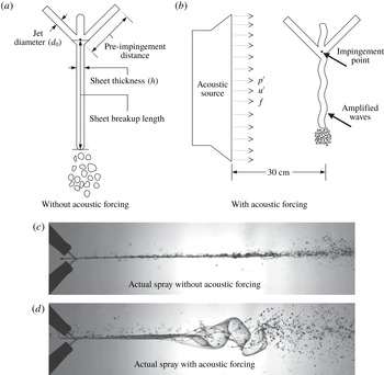
(a,b) Schematics of the liquid sheet with nomenclature of various parameters used (a) without and (b) with acoustic forcing. (c,d) Actual side views of the sheet (c) without and (d) with acoustic forcing.

2 Experimental set-up and methodology
2.1 Liquid sheet formation and acoustic forcing
Figure 1(a) shows the schematic of the side views of the liquid sheet formed by the oblique collision of two similar jets (for reference, the actual spray photograph is also shown in figure 1
c). The sheet parameters and the jet parameters are also shown in figure 1(a). The schematic of the acoustically forced liquid sheet is presented in figure 1(b) (the actual spray photograph is shown in figure 1
d). The liquid sheet is formed using a glycerol–water mixture (80 : 20 by volume) having surface tension
 $0.06487~\text{N}~\text{m}^{-1}$
(measured using a Wilhelmy plate surface tensiometer GBX CAP 26), viscosity 0.04986 Pa s (measured using Anton Paar rotational rheometer MCR-301) and density
 $1205~\text{kg}~\text{m}^{-3}$
. Two identical brass orifices with orifice diameter (
 $d_{0}$
) of 1 mm are used, which form the laminar jets prior to their impact. The impingement angle (
 $2\unicode[STIX]{x1D703}$
) between the jets is
 $90^{\circ }$
and it was kept constant throughout the present work. Experiments are conducted at various Weber numbers (
 $We=\unicode[STIX]{x1D70C}V^{2}d_{0}/\unicode[STIX]{x1D70E}$
, where
 $\unicode[STIX]{x1D70C}$
is the density of the liquid,
 $V$
is the jet velocity and
 $\unicode[STIX]{x1D70E}$
is the surface tension). The Reynolds number (
 $Re=\unicode[STIX]{x1D70C}Vd_{0}/\unicode[STIX]{x1D707}$
, where
 $\unicode[STIX]{x1D707}$
is the dynamic viscosity) for the chosen set of Weber numbers lies between 8 and 175, which ensures the laminar nature of the jets. The corresponding liquid sheet is also laminar and smooth. The sheet is exposed to travelling acoustic (sound) waves over a wide range of sound pressure levels (
 $SPL=50{-}110~\text{dB}\pm 3~\text{dB}$
) and frequencies (
 $f=100{-}1000~\text{Hz}\pm 5~\text{Hz}$
). The acoustic source (speaker) is placed at a distance of 30 cm from the sheet.
A stable liquid sheet is formed first and then it is subjected to the acoustic forcing in each experimental run. The acoustic waves are generated by the sinusoidal signal of varying frequencies in MATLAB audio library using a sine wave generator. The sinusoidal signal is then sent to an audio amplifier (Crown XLI 800) and then to a speaker (Ahuja VS 200). A sound wave is nothing but a longitudinal wave comprising compression and rarefaction of air and it causes the displacement of the air particles in an oscillatory manner. When the liquid sheet is forced with acoustic excitation, there is a transfer of momentum from a layer of air at the interface of the sheet to the liquid sheet. This momentum transfer perturbs and displaces the sheet in a direction normal to its plane, setting up the flapping motion as shown in figure 1(b) and 1(d). A typical perturbation experienced by the liquid sheet is thus proportional to the displacement of air particle in the vicinity.
We use a linear wave propagation formulation to get an estimate of this displacement. Acoustic waves freely propagating in still air displace an air particle with a velocity (
 $u^{\prime }$
) given by (Rienstra & Hirschberg Reference Rienstra and Hirschberg2004)
 $$\begin{eqnarray}\displaystyle & \displaystyle u^{\prime }=\frac{p^{\prime }}{\unicode[STIX]{x1D70C}_{0}c_{0}}, & \displaystyle\end{eqnarray}$$
 $$\begin{eqnarray}\displaystyle & \displaystyle SPL=20\log _{10}\left(\frac{p^{\prime }}{2\times 10^{-5}}\right). & \displaystyle\end{eqnarray}$$
Here,
 $p^{\prime }$
is the root mean square of the acoustic pressure,
 $\unicode[STIX]{x1D70C}_{0}$
is the air density,
 $c_{0}$
is the speed of sound in air and
 $SPL$
is the acoustic sound pressure level. The displacement of the air particle due to the acoustic wave is given by (Rienstra & Hirschberg Reference Rienstra and Hirschberg2004)
 $$\begin{eqnarray}\displaystyle a_{0}=\frac{|u^{\prime }|}{2\unicode[STIX]{x03C0}f}. & & \displaystyle\end{eqnarray}$$
Here,
 $u^{\prime }$
is the velocity perturbation due to the acoustic wave and
 $f$
is the frequency of the wave. The particle displacement is a function of acoustic frequency at constant sound pressure level.
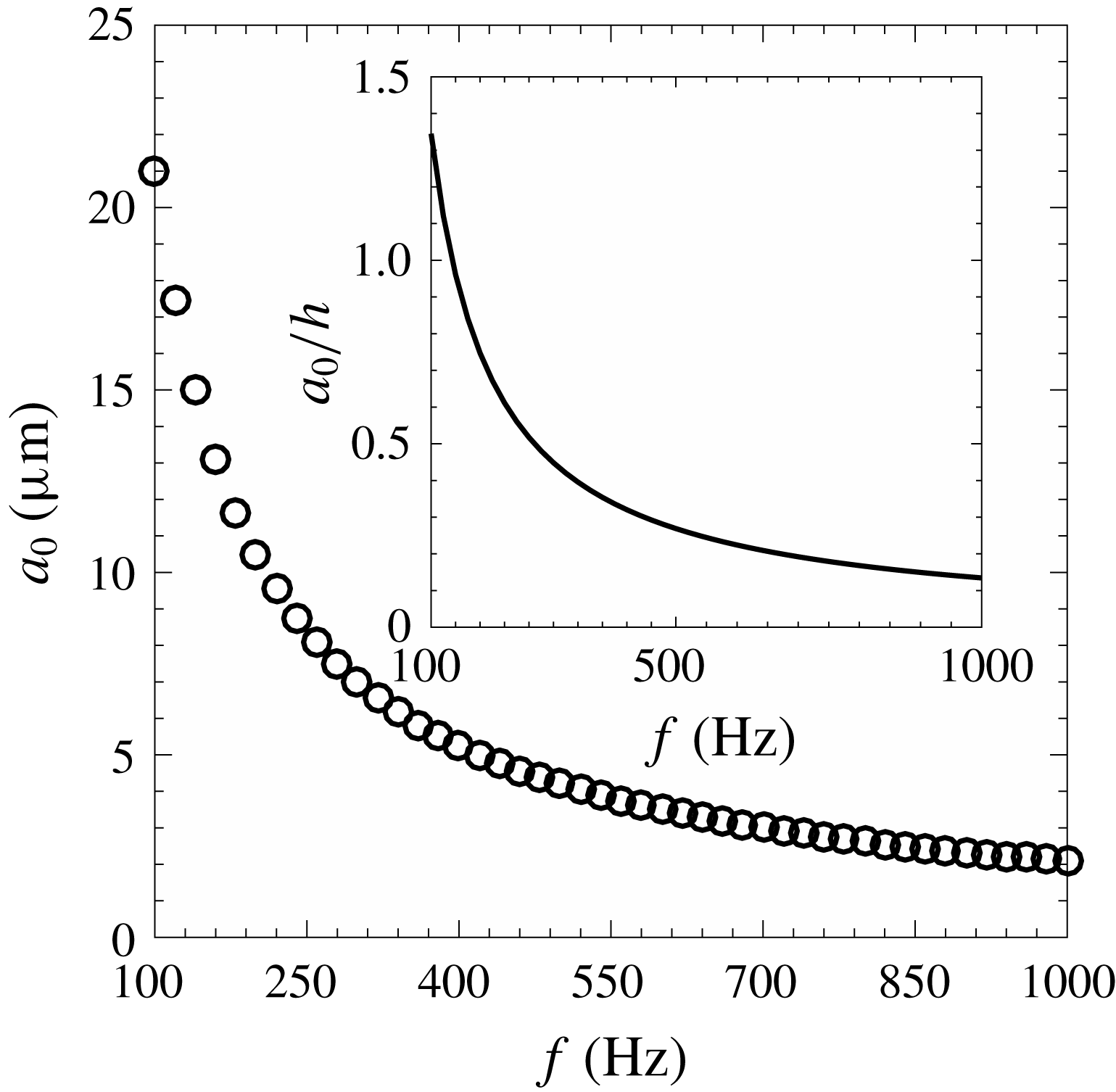
In the present case, we excited the sheet with different frequencies (100–1000 Hz with an interval of 20 Hz) and sound pressure levels (50–110 dB with an interval of 10 dB). Figure 2 shows the variation of the particle displacement or the perturbation amplitude (
 $a_{0}$
) with excitation frequency at 109 dB. For lower frequencies, the particle displacement is high and then decreases with increase in the frequency. The inset in figure 2 shows the particle displacement normalized by the average sheet thickness for
 $We=973$
, which shows that, for the present study, the particle displacement is of the order of the sheet thickness.
Amplitude of the particle displacement (
 $a_{0}$
) due to the propagation of a sound wave as a function of frequency for 109 dB. The inset shows the particle displacement normalized by the average sheet thickness for
 $We=973$
. The typical particle displacement is of the order of the sheet thickness.

2.2 Spray test facility
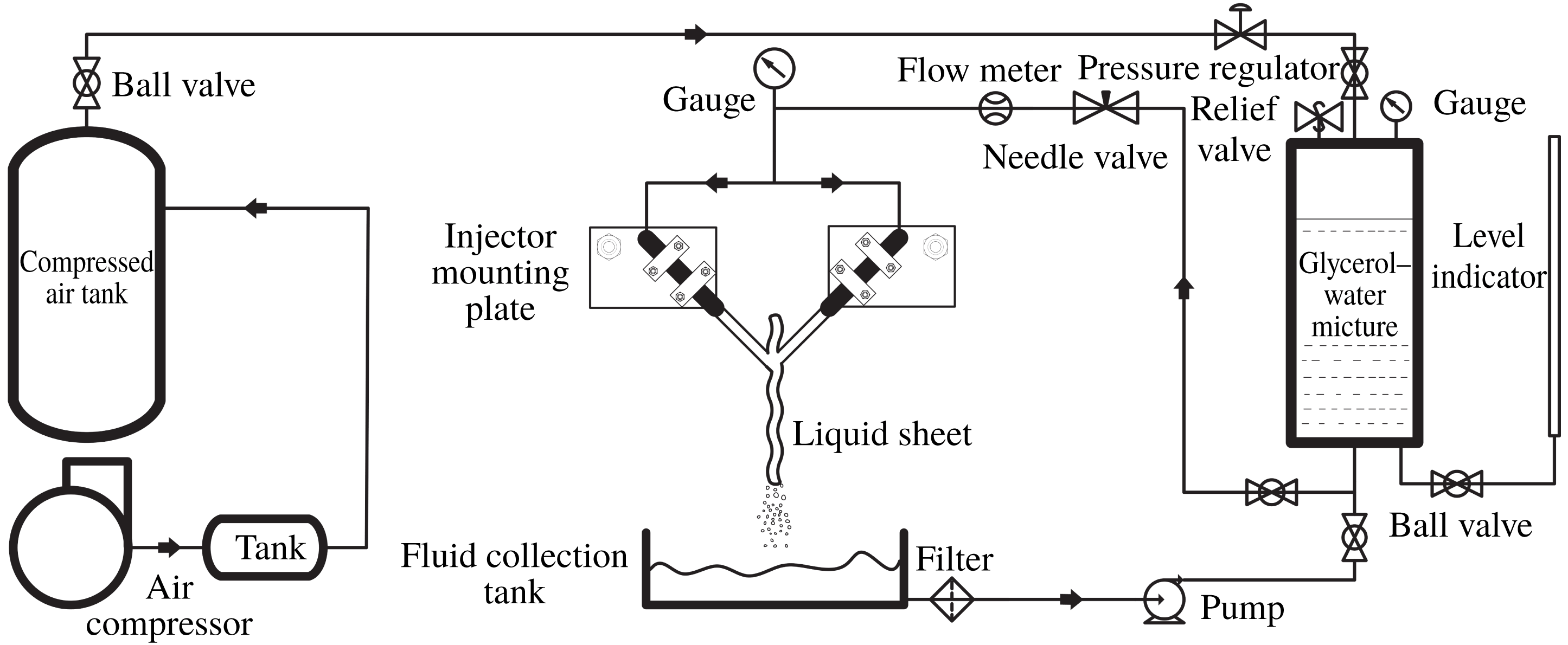
The schematic of the spray test facility is shown in figure 3. The main parts of the test facility are the injector mounting stands, the fluid storage and pressurization system, and the flow control and measurement devices. Two injectors are clamped to two aluminium plates on which the angle between the two jets can be adjusted. One of the plates is mounted on the microscopic traverse while the other is mounted on a stand that has two degrees of freedom in the horizontal plane. The fine adjustment required to form the sheet in a plane perpendicular to the plane containing the jet axes is done by microscopic traverse, which has an arrangement to move the jet in the vertical as well as horizontal plane. The glycerol–water mixture is stored and pressurized in a tank having a 25 litre capacity. Pressurized air is supplied from the air compressor; a pressure of
 $4\times 10^{5}~\text{N}~\text{m}^{-2}$
was maintained in the glycerol–water tank using a pressure regulator (Shavo SR20) during all the experiments. The sprayed fluid was collected in the fluid collection tank and supplied back to the tank using a pump. Flow to the injector was controlled by a needle valve. The volume flow rate of fluid is measured by the rotameter (
 $0.01{-}0.4~\text{l}~\text{min}^{-1}$
, 5 % uncertainty) and the pressure readings were obtained from the pressure gauge (
 $0{-}6.86\times 10^{5}~\text{N}~\text{m}^{-2}$
).
Schematic of the spray test facility.

2.3 Flow visualization and image processing
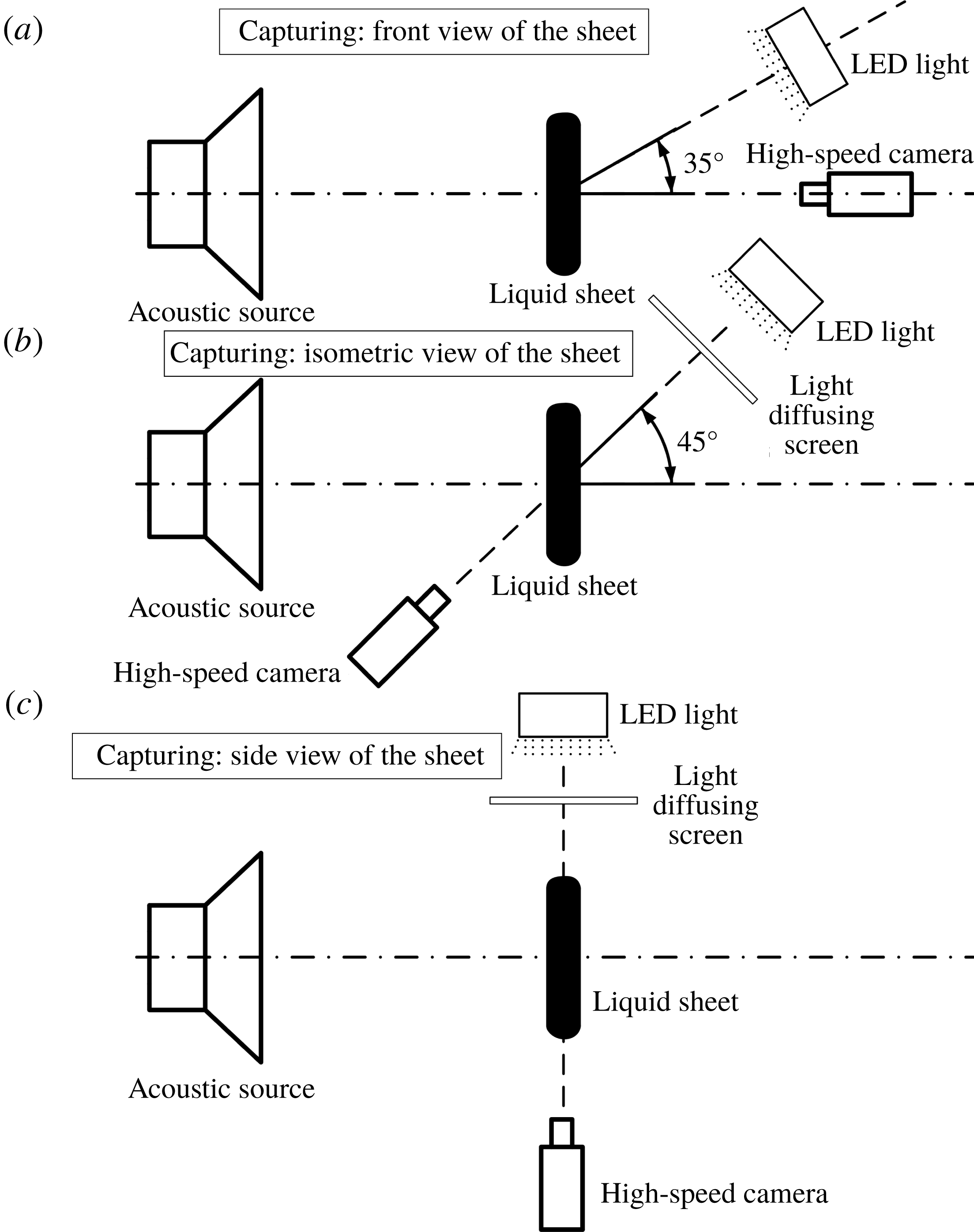
To study the qualitative changes in the sheet breakup process and to measure the effect of acoustic parameters on the sheet dimensions, the sheet visualization without and with acoustic forcing is carried out by a high-speed photography method as shown in figure 4(a). The sheet is illuminated with light from a 100 W light-emitting diode (LED) and the sheet images are captured using a high-speed camera (IDT Motion Xtra NX4S2). The speaker is placed on the central axis, which is perpendicular to the sheet plane, and the high-speed camera is placed on the same axis but opposite to the speaker. Owing to this constraint, the light source is placed at an angle (
 $35^{\circ }$
) to the central axis. The sheet breakup length without forcing (
 $L_{0}$
) and with forcing (
 $L$
) is measured from the front views of the sheet. The sheet breakup length measurement was carried out in the open-source image processing software ImageJ. For each condition, the breakup length is the average of a sequence of 100 sheet images.
Different optical arrangements for visualization of the front view of the liquid sheet (a), the isometric shadowgraphic view (b), and the shadowgraphic side view (c) for measurement of various parameters.

The observation of the front views of the sheet with excitation showed amplified waves on the sheet surface. To reveal the wave dynamics and to discover the origin of the generation of the amplified waves, we captured the isometric views of the sheet by the high-speed shadowgraphy method, as shown in figure 4(b). In figure 4(b), the acoustic source and the sheet position are unchanged (the same as shown in figure 4
a). Only the high-speed camera and the light source were placed at an angle (
 $45^{\circ }$
) to the central axis to capture the isometric views of the sheet. Further, the side views of the sheet are captured by the shadowgraphy method as shown in figure 4(c) mainly to investigate the wave frequency, the maximum wave amplitude and the spatial growth rate. The spatial growth in amplitude is measured from the sheet envelope. The sheet envelope is created using 500 sheet images, which are filtered and overlapped. The wave frequency is measured by tracking the successive wave crests at a fixed location. The drop size measurement is carried out over a fixed region below the sheet using the high-speed shadowgraphy method. The experimental arrangement for the measurement of the droplet size is similar to that of figure 4(b). A special type of long-distance microscopic lens (Questar QM 100) having a resolution of
 $175~\text{pixels}~\text{mm}^{-1}$
is used to capture the droplets. A large number of images (approximately 2000) for each case are used to measure the droplet size. These images are processed in the ImageJ batch processing unit to obtain the mean drop diameters.
Sheet produced by the oblique jet impingement for
 $We=973$
. (a,b) Natural sheet breakup in isometric view (a) and side view (b). (c,d) Acoustically forced sheet (
 $f=120~\text{Hz}$
,
 $SPL=109~\text{dB}$
) in isometric view (c) and side view (d). See also supplementary movie 1, available at https://doi.org/10.1017/jfm.2019.732.

3 Experimental observations
3.1 Interaction of liquid sheet with the acoustic field
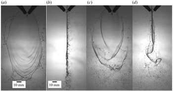
The first major realizable effect of the imposed acoustic field may easily be noted in figure 5. Figures 5(a) and 5(b) show two different views of a flat sheet produced by the oblique jet impingement. The sheet surface is smooth for most of the sheet region while the wave train appears at the bottom edge of the sheet. The ligaments are centrifuged from the thicker rim, leading to bigger drops, and fine droplets are observed at the bottom. Figure 5(b) shows that the sheet lies perfectly in a plane normal to the plane of the jets and so are the droplets at the bottom. This is a classic picture of how a typical flat sheet breaks up in a quiescent ambient. When this liquid sheet is exposed to the transverse acoustic waves, the sheet violently flaps about its mean position and breaks up early, as shown by the instantaneous images in figures 5(c) and 5(d). The acoustic waves hit one of the sheet surfaces facing the speaker, creating an oscillatory pressure differential between the two surfaces of the sheet. This pressure difference, however small it is, is sufficient to result in the acceleration of the sheet perpendicular to its plane. Small-amplitude perturbations are experienced by the sheet at the impingement point of the two jets. These perturbations grow faster and bigger as they move away from the impact point in comparison with a free liquid sheet and create notable differences in the breakup characteristics.
A free liquid sheet develops amplification of unstable waves due to the shear (Kelvin–Helmholtz type instability) when the velocity differential between the sheet and the ambient gas is sufficiently large. The flapping behaviour becomes intense if the sheet velocity with respect to the ambient gas increases. The acoustic forcing provides additional perturbations to the inherent instabilities associated with the liquid sheet breakup, resulting in violent flapping like a flag at much lower sheet velocities. Large-amplitude flapping results in further wrapping and stretching of the liquid sheet, centrifugal instabilities due to the curvature effects, random perforations prior to the breakup location, and shedding of the droplets out of the original sheet plane, as depicted in figures 5(c) and 5(d).
Evolution of the sheet breakup during the initial instants when exposed to the acoustic excitation for
 $We=608$
,
 $f=120~\text{Hz}$
and
 $SPL=109~\text{dB}$
. The first image (a) corresponds to the sheet in the unexcited condition. The time interval between successive images is 2 ms. See also supplementary movie 2.

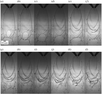
Figure 6 shows images of initial instants during the transition from the natural breakup mode to the forced breakup mode of a smooth sheet. In these images, the darkness of the waves on the sheet surface is proportional to the wave amplitude. The first image of the sequence (figure 6 a) is the natural or unforced breakup just prior to the application of the acoustic field. It shows a perfectly smooth sheet bounded by the rim and the wavy pattern only at the bottom. It may be noted that the whole sheet, although exposed to the acoustics, is not affected by it immediately (figure 6 b,c). The prominent wave pattern develops gradually from figure 6(d) onwards. Weak waves appear on the otherwise smooth sheet from figure 6(d) and the wave pattern establishes thereafter. It is also clear that the waves travel away from the impingement point. The perturbations imposed by the acoustic forcing create the oscillatory motion of the impingement point and these perturbations grow in amplitude spatially as the wave progresses (figure 6 d–g). This feature is very important and will be used in § 4 while applying the stability theory to this phenomenon.
As the waves reach near the edge of the sheet, the wavelength decreases, resulting in a decrease in the wave speed. A larger differential between the wave velocity and the velocity of the fluid particle leads to fragmentation via flapping that looks quite complex from figure 6(l). Holes/perforations may be observed in the sheet near to the rim and the lower half of the sheet. The phenomenon of the formation of holes is found to be intermittent and random. Further, the frequency of hole formation is also low and hence this phenomenon cannot be regarded as a consequence of the sheet instabilities. The possible causes for the formation of holes may be the local stretching as well as thinning of the sheet, chemical inhomogeneities (as a result of the working fluid being a mixture) and the hygroscopic nature of glycerol. As the wave train reaches the side edges of the sheet, which are fairly close to the impact point as compared to the bottom edge, one may note the sudden ejection of the rim in the form of a thread. This thread ultimately undergoes secondary breakup of Rayleigh type, as is evident in figure 6. The broken rim is re-established and the phenomenon repeats periodically. The presence of large-amplitude waves near the breakup location and shedding of liquid mass in the form of droplets retracts the sheet and the breakup length consequently decreases. This phenomenology will be helpful in analysing the physical processes and the changes in the sheet characteristics.
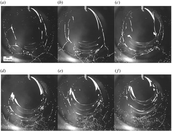
Instantaneous images showing the effect of acoustic frequency on the wave pattern and the sheet structure at 109 dB for
 $We=973$
: (a) unexcited, (b) 120 Hz, (c) 220 Hz, (d) 320 Hz, (e) 420 Hz and (f) 520 Hz. See also supplementary movies 3 and 4.

3.2 Effect of acoustic parameters
3.2.1 Effect of forcing frequency
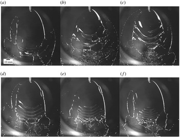
Figure 7 shows typical images of the liquid sheet surface subjected to acoustic excitation of varying forcing frequencies at a constant sound pressure level. The white bands on the sheet surface indicate the presence of waves; it is worth mentioning at this point that the intensity of the white bands signifies the amplitude of the waves. As such, the white bands appear only when the waves attain a certain amplitude. The first image represents the unexcited condition (figure 7 a) with all its characteristic features. The effect of the acoustic frequency on the sheet characteristics may be noted from figure 7(b–f), which is essentially due to the changes in the wave pattern. For lower sound frequency, the waves appear closer to the point of jet impingement and they seem to be much brighter (figure 7 b,c). This indicates that the wave amplitude grows rapidly at lower frequencies. Figure 7 also shows that the wavelength and amplitude of the wave train decrease for increasing forcing frequencies (discussed later in § 3.3). The first distinguishable effect of the acoustic forcing is reduction in the sheet breakup length. The reduction in the sheet breakup length is more pronounced at lower frequencies as compared with the higher frequencies (for example, compare figure 7 b and e). For lower frequencies, the sheet experiences violent flapping with large-amplitude waves relatively closer to the impingement point, leading to the early attainment of the critical sheet thickness at which breakup occurs. The variation in the breakup length with frequency provides a rational measure to determine the response of the sheet to the external acoustics.
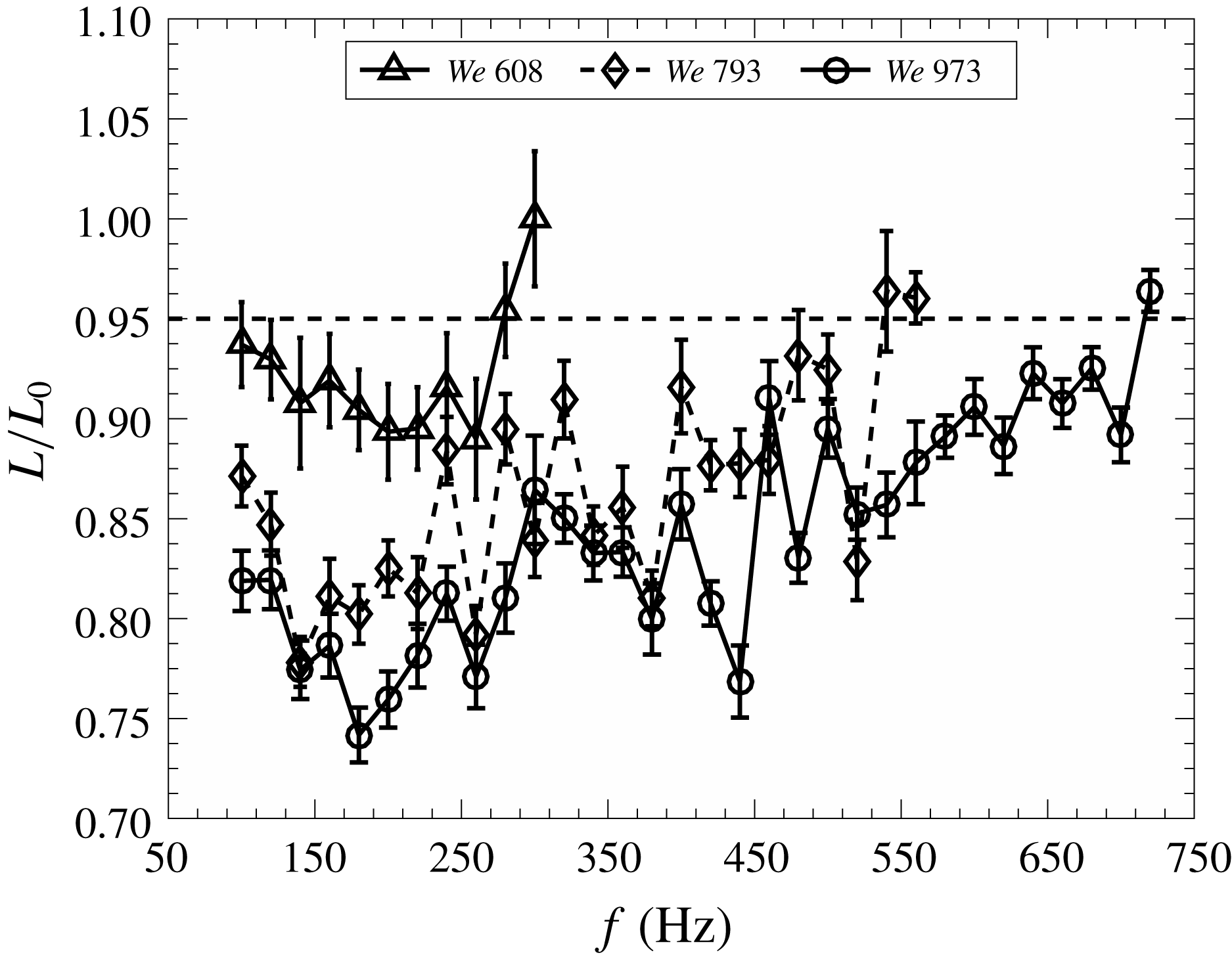
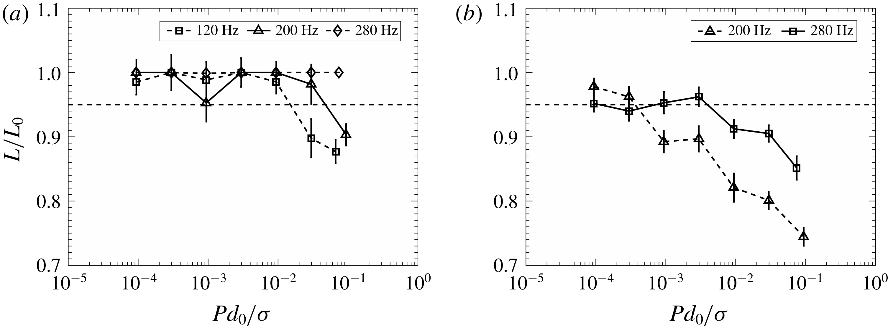
Effect of acoustic frequency on the sheet breakup length at 109 dB. The horizontal dashed line represents 5 % reduction in the mean breakup length of the free liquid sheet. Points below this line indicate the frequencies causing perceptible response from the sheet.

Figure 8 shows the variation of non-dimensional breakup length with excitation frequency for different Weber numbers. The non-dimensional breakup length is the ratio of the average breakup length (
 $L$
) in the presence of acoustic forcing and the average breakup length of a free sheet (
 $L_{0}$
). As pointed out earlier, figure 8 quantitatively shows a gradual increase, although non-monotonic, in the sheet breakup length with excitation frequency. The sheet is said to be responding to those frequencies when the breakup length of the excited sheet reduces by more than 5 % of the breakup length of the free sheet for similar flow conditions (this demarcation is shown by a dashed line in figure 8). We observe that the overall uncertainty in the measurement of sheet breakup length is nearly 3 %. Hence, a 5 % measure is chosen to represent the effect of acoustics, similar to Mulmule et al. (Reference Mulmule, Tirumkudulu and Ramamurthi2010). The most interesting feature of figure 8 is the existence of a continuous spectrum of acoustic frequencies which influences the breakup and the sheet characteristics. This observation is in contrast with the observation of discrete frequencies by Mulmule et al. (Reference Mulmule, Tirumkudulu and Ramamurthi2010) and Dighe & Gadgil (Reference Dighe and Gadgil2018) for water sheets. Water, being a relatively low-viscosity liquid, produces turbulent sheets for similar Weber numbers. It may possibly be that, due to the turbulent nature of the liquid sheet, the earlier works (Mulmule et al.
Reference Mulmule, Tirumkudulu and Ramamurthi2010; Dighe & Gadgil Reference Dighe and Gadgil2018) were unable to capture the subtle effect of acoustics on the sheet characteristics resulting in discreteness in the frequencies. Further, it is evident from figure 8 that the range of frequencies affecting the sheet breakup increases with increase in the Weber number. For example, the sheets respond up to frequencies of approximately 300 and 720 Hz for Weber numbers of 608 and 973, respectively. The reduction in the breakup length for a given frequency also increases with increase in the Weber number.
The acoustic pressure difference across the sheet displaces and accelerates the sheet normal to its plane. The force balance on the sheet may be expressed as
 $$\begin{eqnarray}\displaystyle P\cos (\unicode[STIX]{x1D714}t)A=Ah\unicode[STIX]{x1D70C}\frac{\text{d}^{2}x}{\text{d}t^{2}}. & & \displaystyle\end{eqnarray}$$
Here,
 $P$
is the pressure difference across the sheet,
 $\unicode[STIX]{x1D714}=2\unicode[STIX]{x03C0}f$
is the frequency,
 $A$
is the sheet area,
 $h$
is the sheet thickness,
 $\unicode[STIX]{x1D70C}$
is the liquid density and
 $h$
is the sheet displacement along the
 $x$
axis (perpendicular to the sheet plane). To get the characteristic sheet displacement
 $x$
, equation (3.1) is integrated:
 $$\begin{eqnarray}\displaystyle x\sim \frac{P\cos (\unicode[STIX]{x1D714}t)}{\unicode[STIX]{x1D70C}h\unicode[STIX]{x1D714}^{2}}. & & \displaystyle\end{eqnarray}$$
For a fixed sound pressure level, the relation between the sheet displacement and the frequency can be expressed as
 $$\begin{eqnarray}\displaystyle x\sim \frac{1}{\unicode[STIX]{x1D714}^{2}}. & & \displaystyle\end{eqnarray}$$
Equation (3.3) shows that the sheet displacement varies inversely with the square of the forcing frequency.
From figure 2 and equation (2.3), we note that the air particle displacement also varies inversely with the square of the frequency for a given sound pressure level. Consequently, the sheet displacement may be considered to be directly proportional to the displacement of the air particle due to the sound wave. From the linear wave propagation theory, we know how the pressure perturbations translate into particle displacement. There exists a resistance from the sheet when this particle displacement is transferred to the sheet. Since the sound pressure levels are very small, the sheet perturbations are also very small near the impingement point. We could not measure these sheet displacements (and the acoustic impedance) due to the limitation of the camera resolution. Hence, we consider the air particle displacement (
 $a_{0}$
) as the characteristic displacement for the rest of the analysis. As the forcing frequency increases, the characteristic sheet displacement or the perturbation magnitude at the impingement point decreases rapidly for a given sound intensity and hence the sheet stops responding to the acoustic excitation. This is the reason for the high reduction in the sheet breakup length at lower frequencies than at higher frequencies.
Cutoff frequencies based on the sheet breakup length reduction criterion at 109 dB.

The frequency at which the sheet stops responding to the acoustic field is named the cutoff frequency (
 $\unicode[STIX]{x1D714}_{c}$
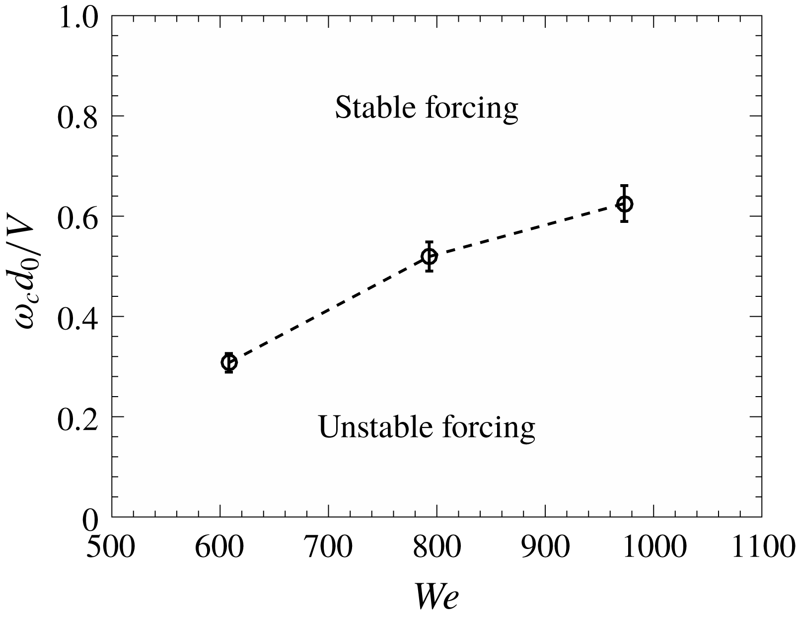
). The response of the sheet is characterized in terms of reduction in the sheet breakup length. If the reduction in the sheet breakup length is more than 5 %, it is said that the forcing is unstable and the sheet responds to the acoustic field. The forcing is said to be stable if the reduction in the breakup length is less than 5 %. Figure 9 shows that the cutoff frequency increases with the increase in the Weber number. It is known that with increase in the Weber number the sheet thickness decreases and the sheet displacement is inversely proportional to the sheet thickness at a fixed sound pressure level (3.2). Hence, for a liquid sheet with higher Weber number, a sheet displacement of relatively lower magnitude is also enough to extract a tangible response from the sheet. Thus, the range of frequencies over which the sheet responds is an increasing function of Weber number. The cutoff frequency with more fundamental criterion will be discussed in § 4 dedicated to the comparison with theoretical predictions.
Effect of sound pressure level on the sheet structure for
 $f=120~\text{Hz}$
and
 $We=973$
: (a) unexcited, (b) 70 dB, (c) 80 dB, (d) 90 dB, (e) 100 dB and (f) 109 dB.

3.2.2 Effect of sound pressure level
Increase in the sound pressure level (
 $SPL$
) essentially exerts more force, causing larger initial transverse perturbation of the sheet. Instantaneous images of the sheet with
 $We=973$
and subjected to varying acoustic pressures at a constant frequency are shown in figure 10. The effect of
 $SPL$
is exactly the reverse of that of frequency. It may be noted from figure 10 that large-amplitude waves due to sheet flapping become prominent as the
 $SPL$
increases. The spatial growth of waves is faster, resulting in large-amplitude waves closer to the impingement point at higher
 $SPL$
. Consequently, the sheet breakup length reduces significantly at higher sound pressure levels. Similar qualitative effects of frequency and perturbation amplitudes were observed by Crapper et al. (Reference Crapper, Dombrowski and Pyott1975) in the case of mechanically vibrated fan spray nozzles.
The non-dimensional breakup length is plotted against the non-dimensional sound pressure level at various frequencies in figure 11. The non-dimensional sound pressure is
 $Pd_{0}/\unicode[STIX]{x1D70E}$
, where
 $P$
is the root mean square pressure,
 $d_{0}$
is the nozzle diameter and
 $\unicode[STIX]{x1D70E}$
is the surface tension of the glycerol–water mixture. The results suggest that the sheet response at a particular sound pressure level depends on the forcing frequency. Figure 11 also shows that there exists a threshold sound pressure level below which the sheet is essentially unaffected. For low Weber number (
 $We=608$
, figure 11
a), the sheet shows significant reduction in the breakup length only at 120 Hz and 200 Hz. For other frequencies (280 Hz and more), the reduction in the sheet breakup length is not significant (less than 5 %) over the entire range of
 $SPL$
tested in the present work. However, the sheet responds to 280 Hz at certain
 $SPL$
when the Weber number increases to 973, as shown in figure 11(b).
If we assume that the sheet responds above a certain critical sound pressure level for a fixed flow condition, then this critical pressure varies directly with the square of the frequency, as observed in (3.2), that is,
 $$\begin{eqnarray}\displaystyle P\sim \unicode[STIX]{x1D714}^{2}. & & \displaystyle\end{eqnarray}$$
For example, for
 $We=608$
at 120 Hz (figure 11
a) the sheet shows significant response at non-dimensional sound pressure level of 0.03, but for 200 Hz the non-dimensional sound pressure level is 0.1. Similarly, for
 $We=973$
(figure 11
b), the sheet shows a significant reduction in the breakup length for 200 Hz and 280 Hz beyond non-dimensional sound pressure level of 0.001 and 0.01, respectively. This observation is consistent with the earlier work on turbulent sheets (Mulmule et al.
Reference Mulmule, Tirumkudulu and Ramamurthi2010; Dighe & Gadgil Reference Dighe and Gadgil2018). If the non-dimensional acoustic intensity is expressed as
 $a_{0}\unicode[STIX]{x1D714}/V$
, then it decreases with increase in the forcing frequency (
 $\unicode[STIX]{x1D714}$
). Increase in the acoustic intensity does not necessarily extract a response from the sheet because of its coupled nature with the forcing frequency. Hence, there exists a critical
 $SPL$
and cutoff frequency which limit the envelope of the sheet response.
Variation in the sheet breakup length with sound pressure level at a given forcing frequency for (a)
 $We=608$
and (b)
 $We=973$
.

3.3 Effect on the drop formation process
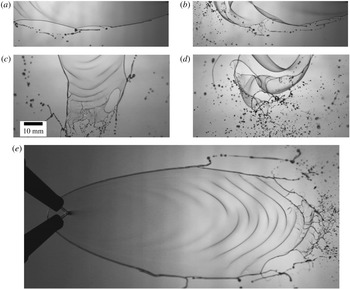
The ultimate interest lies in the fragmentation of a sheet in the form of ligaments and droplets and the effect of external perturbations on this process. Figure 12 is given to depict the characteristic features of sheet disintegration at the rim and at the bottom edge in the absence and presence of acoustic forcing. A thicker rim of the sheet (figure 12 a) develops cusps and the cylindrical ligaments stretch out from the cusps, which finally break into droplets by the classical capillary instability (Rayleigh–Plateau instability). At the bottom edge, waves are clearly visible (figure 12 c). The wavy nature of the sheet is a result of shear instability of the liquid sheet moving in the still air. The amplitude of these waves grows rapidly as they move towards the sheet edge. The sheet disintegrates into fine drops as the waves attain the critical amplitude and breaks as shown in figure 12(c). A closer observation of the bottom part of the sheet points out the presence of the corrugations of the wave crests. At the sheet bottom, due to the amplification of waves, the sheet is accelerated perpendicular to its surface and this acceleration leads to the Rayleigh–Taylor instability producing corrugations of the wave crests. This type of secondary sheet destabilization mechanism is described as the ‘wavy corridor’ by Bremond et al. (Reference Bremond, Clanet and Villermaux2007).
(a–d) Changes in the droplet formation mechanism in the presence of external acoustics. The sheet rim and sheet bottom edge breakup without forcing (a,c) for
 $We=608$
and with forcing (b,d) for
 $We=608$
,
 $f=120~\text{Hz}$
and
 $SPL=109~\text{dB}$
. Panel (e) shows the wavy corridor
 $We=608$
,
 $f=440~\text{Hz}$
and
 $SPL=109~\text{dB}$
. The scale shown in panel (c) is the same for all.

Figure 12(b) shows the breakup of the sheet rim in the presence of acoustic forcing. The amplified disturbance propagating from the impingement point arrives at the sheet rim and initiates the rim breakup. It can be clearly observed that the short and thin liquid columns separate directly from the rim and the cusp structure almost disappears. The sites of ligament detachment also increase as compared to the preferential cusp locations observed in the case of the free sheets. However, the ligaments further undergo breakup due to the capillary instability. Also, the curved rim structure is observed due to the amplification of the waves. The sheet flaps vigorously under the action of acoustics and the waves of high amplitude significantly affect the breakup at the bottom edge as shown in figure 12(d). Large-amplitude waves form the curvatures on the sheet surface that finally result in stretching and thinning of a liquid sheet. Figures 12(b) and 12(d) show the presence of fine droplet clusters formed due to the rupture of the liquid sheet in forced conditions. At lower forcing frequencies, the presence of the wavy corridor is not observed. However, at higher forcing frequencies near to the cutoff, the amplitude of the waves is relatively small and a large number of waves are observed on the sheet (as shown in figure 12 e). Also, the sheet disintegrates due to the secondary instability involving the lateral corrugations, which may be observed at the bottom part.
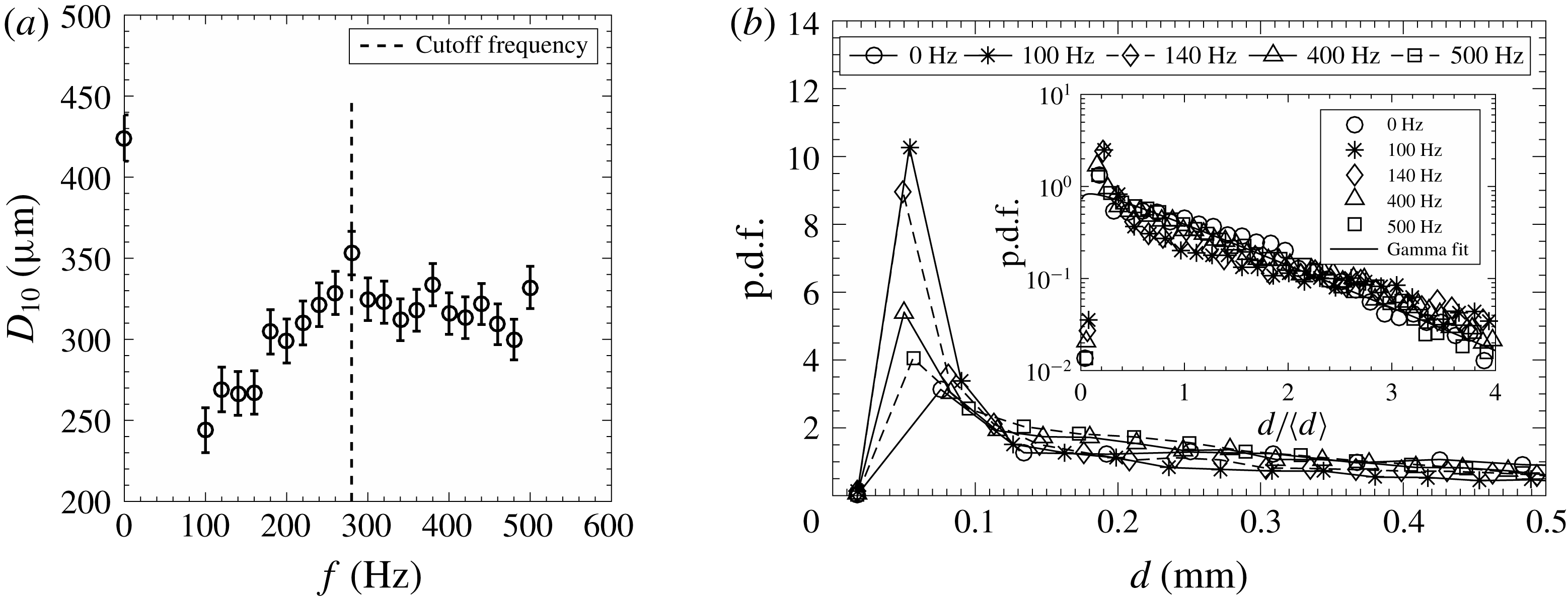
Effect of the forcing frequency on the mean droplet size (a) and the size distribution (b) for
 $We=608$
at a fixed
 $SPL$
level of 109 dB. The inset in (b) shows the non-dimensional drop size distribution, which is well represented by the Gamma distribution.

Flapping of the sheet due to the acoustic forcing essentially alters the mean drop size of the resulting spray. The mean droplet size (
 $D_{10}$
) and the drop size distribution for
 $We=608$
without and with forcing are shown in figure 13. The mean drop diameter reduces in the presence of excitation (figure 13
a) and a significant reduction is observed at frequencies lower than the cutoff frequency. The mean droplet size increases with increase in forcing frequency till the cutoff frequency is reached. After the cutoff frequency, the mean drop size, although much lower than that for the unforced condition, saturates with no significant variation with frequency. Interestingly, the peak of the drop size distribution shifts towards lower drop size under forcing conditions. This is an indication of significant increase in finer droplets due to the kind of sheet rupture seen in figure 12(d). The peak gradually approaches the free sheet condition with increase in frequency across the cutoff frequency, as shown clearly in figure 13(b). The sheet breakup at frequencies near the cutoff frequencies and higher is influenced by the secondary instability mechanism (wavy corridor) similar to the natural breakup (figure 12
c and e). This makes the dimensional drop size distribution (figure 13
b) less sensitive to the forcing frequencies and it approaches that observed for the unexcited sheet. However, at lower frequencies, the high amplitude of the peak shows the dominance of a different type of mechanism (figure 12
d) leading to very fine droplets and the dimensional drop size distribution is sensitive to the forcing.
The inset in figure 13(b) shows the probability density functions (p.d.f.s) of the drop size without acoustic forcing and for various forcing conditions. The droplet sizes are normalized by the mean diameter (
 $D_{10}$
). The drop size distribution is unaltered by the external forcing and can be well represented by the Gamma distribution curve. The Gamma distribution is given by
 $$\begin{eqnarray}\displaystyle P(X)=\frac{n^{n}X^{n-1}\text{e}^{-nX}}{\unicode[STIX]{x1D6E4}(n)}. & & \displaystyle\end{eqnarray}$$
Here,
 $X=d/\langle d\rangle$
,
 $P(X)$
is p.d.f. and
 $n$
is the order or index. This result is in line with the earlier studies on mechanically (Bremond et al.
Reference Bremond, Clanet and Villermaux2007) and acoustically (Mulmule et al.
Reference Mulmule, Tirumkudulu and Ramamurthi2010) excited circular sheets, except for the value of
 $n$
. The value of
 $n$
is sensitive to the injector configuration and corrugations on the liquid thread from which the droplets are formed. The value of
 $n$
in the present study is 1.1 as compared to 4–5 in Bremond et al. (Reference Bremond, Clanet and Villermaux2007) and 2.2 in Mulmule et al. (Reference Mulmule, Tirumkudulu and Ramamurthi2010). In the case of a circular sheet, the droplets are formed due to secondary instability alone, but in the present case the droplets are formed due to rim instability as well as the secondary instability. The lower value of
 $n$
suggests that the ligaments are highly corrugated and the size distribution is broader. Further, an
 $n$
value close to one (1.1) shows that the size distribution may also be approximated by an exponential function.
3.4 Wave characteristics
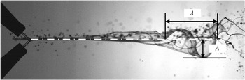
We measure various characteristics of the waves emanating and growing from the point of jet impact to understand the instability mechanisms. Typical wave measurements are shown in figure 14. It was shown earlier (§§ 3.3 and 3.4) that the forcing frequency has a critical role in terms of the resulting sheet characteristics. The forcing frequency is even more critical in the case of the acoustic perturbation, as the perturbation amplitude is directly linked to the frequency for a given dB level, unlike the independent control feasible in the mechanical vibrator (Bremond et al. Reference Bremond, Clanet and Villermaux2007). High-speed shadowgraphic images are used to measure the wave frequency. At a fixed location just before the wave breaks, the movement of the wave crest is monitored for the measurement of the wave frequency. The number of frames present between two successive wave crests passing a fixed location is measured and the time period of the wave is calculated from the average value of a number of frames. The frequency of the wave is measured from the average time period of the wave.
Representation of the wave amplitude (
 $A$
) and wavelength (
 $\unicode[STIX]{x1D706}$
).

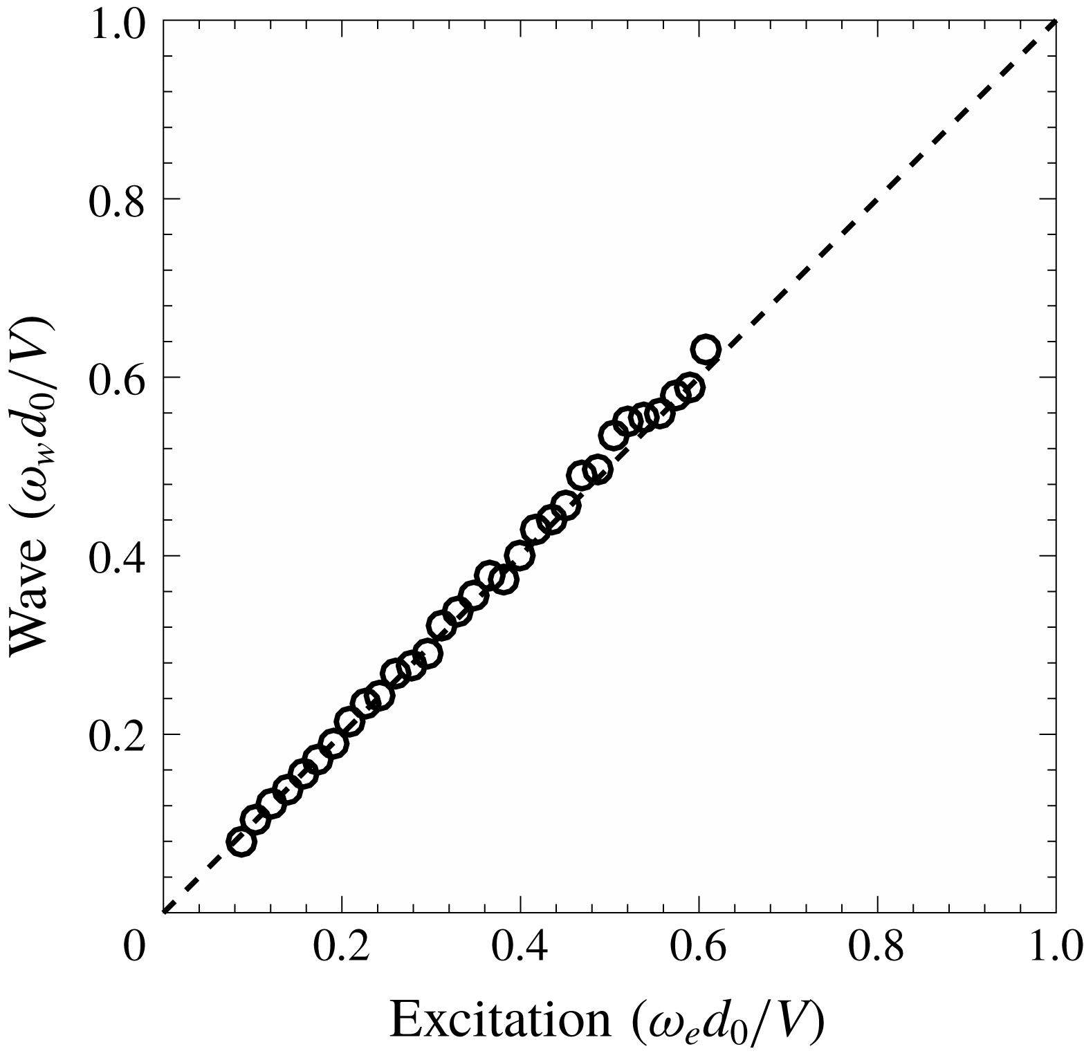
Figure 15 shows the typical variation in the non-dimensional sheet wave frequency (
 $\unicode[STIX]{x1D714}_{w}d_{0}/V$
) as a function of non-dimensional excitation frequency (
 $\unicode[STIX]{x1D714}_{e}d_{0}/V$
) for
 $We=973$
at 109 dB. The observed trend is linear, as shown by the dashed line in figure 15 with slope of
 $45^{\circ }$
. It is clear that the wave frequency, in the presence of the acoustic forcing, is controlled by the external excitation frequency, and is the same as that of the imposed frequency. The perturbations are received by the impingement point with the excitation frequency and correspondingly the sheet waves are forced to propagate with the imposed frequency on the sheet. We demonstrated this feature exclusively since it will be handy in assessing the spatial growth of instability waves in § 4.
Effect of the excitation frequency on the frequency of sheet flapping (
 $We=973$
and
 $SPL=109~\text{dB}$
). The unstable waves are forced to adapt to the forcing frequency.

Sheet envelopes for different Weber numbers depicting the effect on wave amplification at
 $SPL=109~\text{dB}$
(
 $a_{0}=11.7~\unicode[STIX]{x03BC}\text{m}$
) and
 $f=200~\text{Hz}$
:
 $We=608$
(a), 793 (b) and 973 (c).

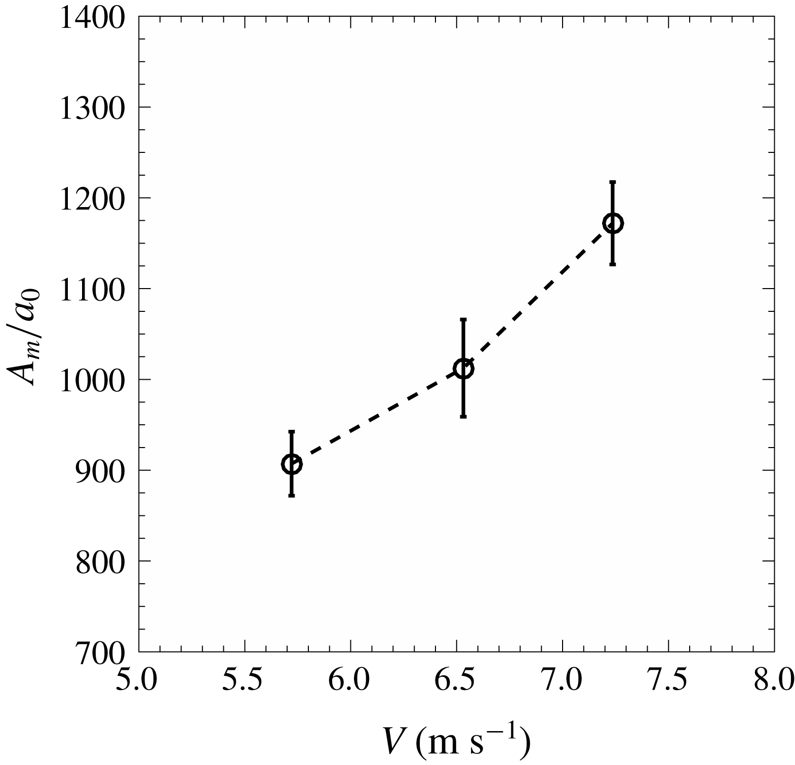
Maximum wave amplitude as a function of jet velocity at 120 Hz and 109 dB. The characteristic displacement of an air particle is used for normalizing the maximum amplitude.

The envelopes of sheet flapping for a given acoustic excitation are shown in figure 16 for different Weber numbers. Figure 16 essentially shows the effect of increasing liquid velocity in the sheet on the growth of imposed perturbations. The sheet envelope is obtained by overlapping a sequence of 500 sheet images. The amplitude of sheet flapping increases with the increase in the Weber number or the jet velocity. As discussed earlier, increase in the sheet velocity leads to greater velocity difference between the fluid and the wave as the waves approach the edge of the sheet. This leads to more intense flapping of the sheet, resulting in larger amplitude of the first antinode, as seen in figure 16. This observation is in line with the observation reported by Bremond et al. (Reference Bremond, Clanet and Villermaux2007) wherein they perturbed only the impact point. Such similarity between these two configurations indicates that the effect of acoustic disturbance on the sheet dynamics may be seen as the spatially developing instability originated from the perturbations at the impingement point.
A more quantitative effect of liquid velocity on the growth of amplitude with respect to the initial perturbation is shown in figure 17. Here, the initial perturbation is assumed to be the displacement of the air particle (
 $a_{0}$
) corresponding to the given acoustic parameters (refer figure 2). The maximum non-dimensional wave amplitude increases significantly with increase in the liquid velocity. It is shown later in § 4 that this maximum amplification is predictable using the linear theory.
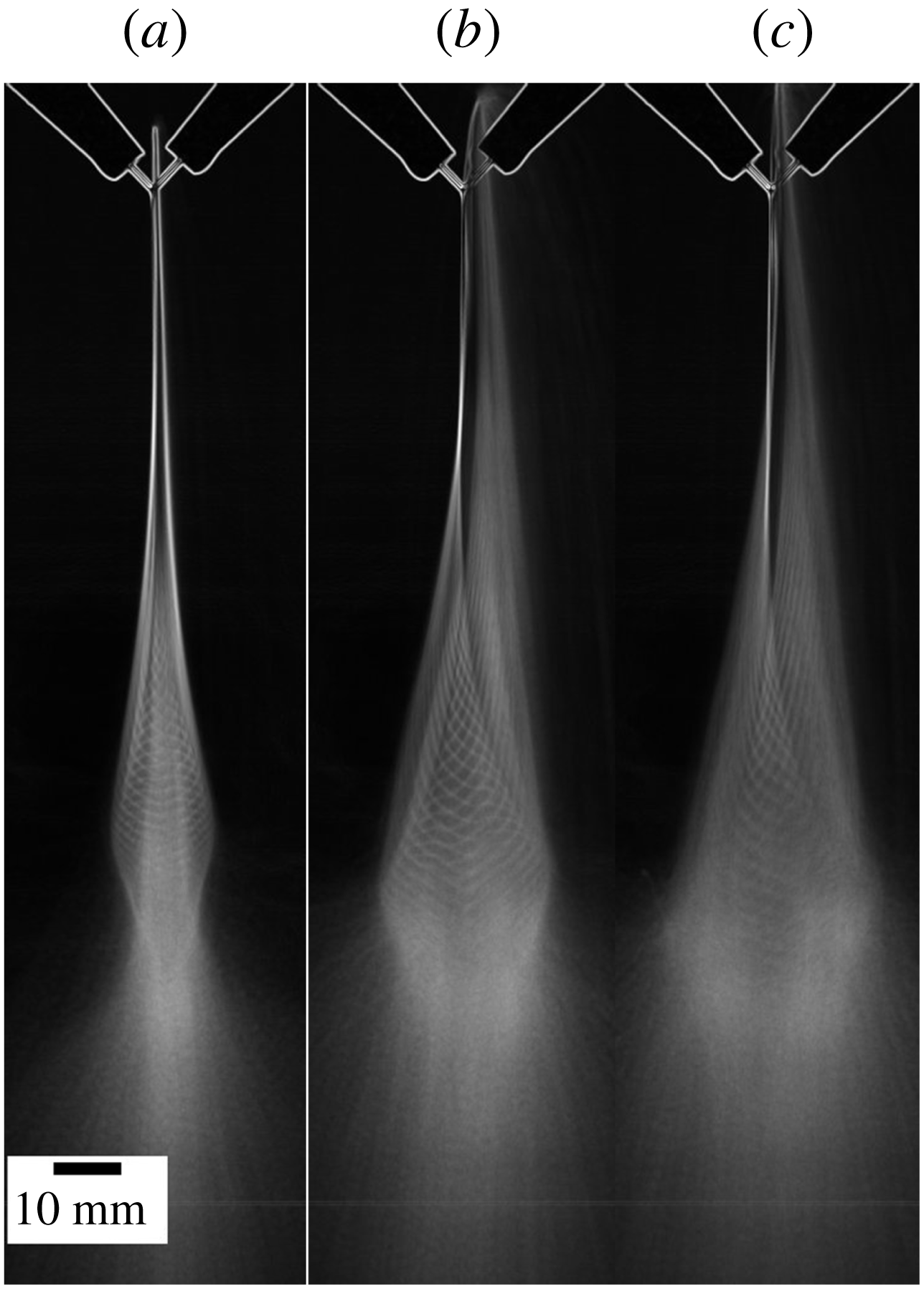
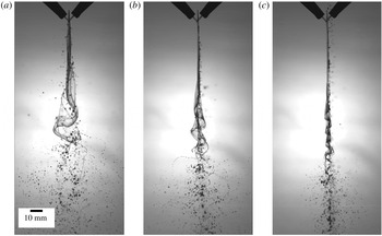
Qualitative effect of forcing frequency on wave amplitude for
 $We=608$
,
 $SPL=109~\text{dB}$
and
 $f=120~\text{Hz}$
(a), 220 Hz (b) and 320 Hz (c). See also supplementary movies 5 and 6.

The frequency of imposed acoustics has a critical role in dictating the wave dynamics and ultimately altering the sheet characteristics as observed in the previous section. Increase in the forcing frequency for a given sound intensity and Weber number suppresses the growth of the waves as depicted in figure 18. As the frequency is increased in figure 18, a violently flapping sheet with large amplitudes gradually turns into a vibrating membrane. The associated changes in the sheet length, the droplet size and their trajectories are also evident from figure 18.
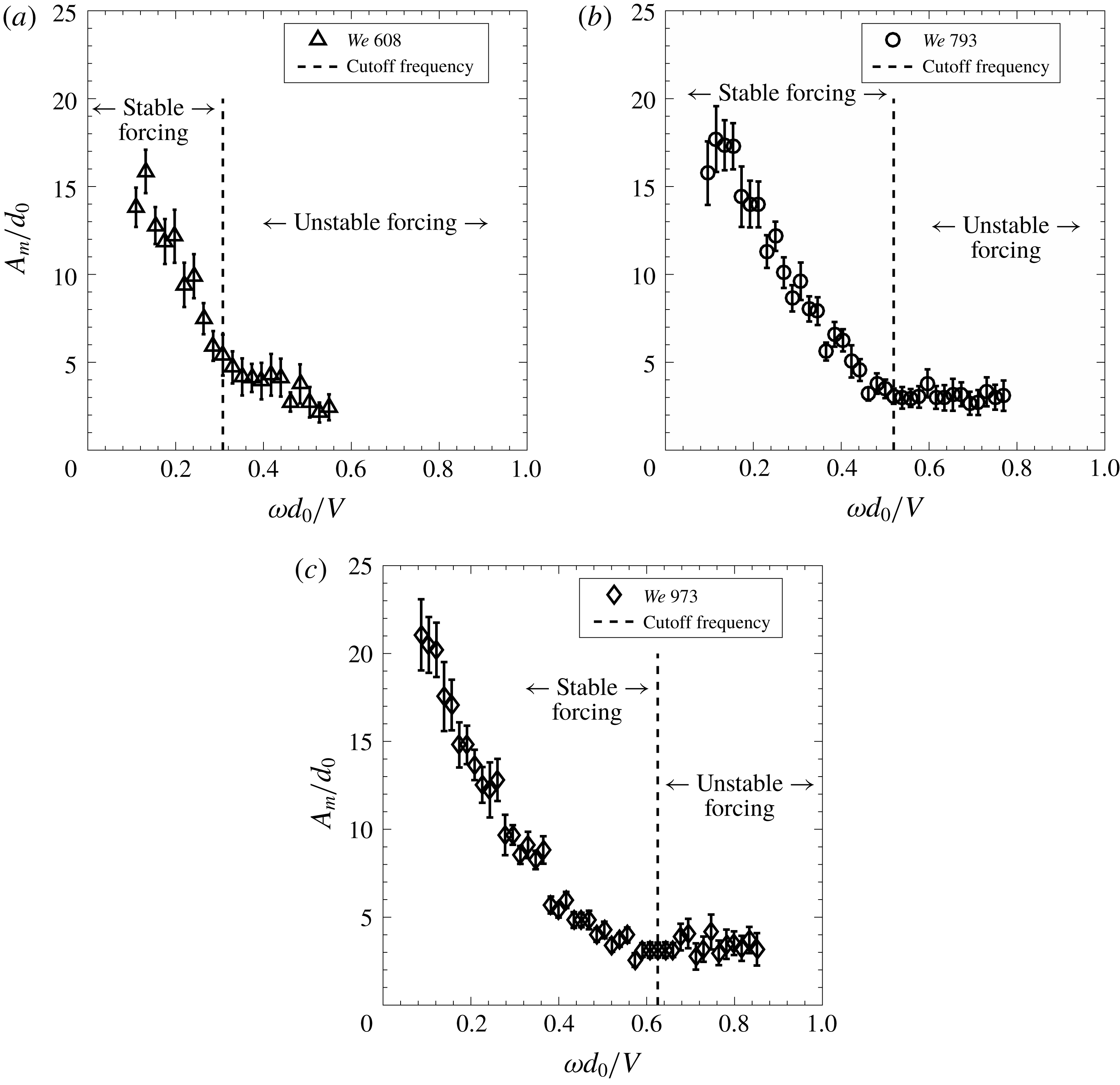
Maximum wave amplitude as a function of non-dimensional frequency at 109 dB: (a)
 $We=608$
, (b)
 $We=793$
and (c)
 $We=973$
.

In order to understand the frequency dependence of the sheet characteristics, we attempt to quantify the maximum wave amplification as a function of forcing frequency. The variation in non-dimensional maximum amplification of the waves (
 $A_{m}/d_{0}$
) with acoustic frequency is shown in figure 19 for various Weber numbers. Jet diameter is used for normalizing the maximum amplitude because the initial sheet perturbation (
 $a_{0}$
) is not a controllable parameter; rather, it varies inversely with the frequency itself. For all Weber numbers, the reduction in the maximum wave amplitude with excitation frequency is evident at lower frequencies from figure 19. After a certain forcing frequency, the maximum wave amplitude saturates with no further appreciable change in it. If we superimpose the cutoff frequency as defined based on the breakup length criterion in figure 19, one may notice that the maximum wave amplitude typically saturates after the cutoff frequency. The cutoff frequency is the frequency beyond which the external acoustics does not have much influence on the sheet characteristics, like breakup length and mean drop size. This means that the sheet characteristics depend on the absolute maximum amplitude and not on the growth of amplitude with respect to the initial perturbation. Another important feature from figure 19 is that the saturation value of the maximum amplitude at the cutoff frequency is approximately the same for different Weber numbers. This shows that the sheet ceases to show variations in its characteristics at a unique value of maximum wave amplitude for the present injector configuration. In this sense, the regions across the cutoff frequencies are defined as stable and unstable forcing as shown in figure 19 (and 9 as well). We shall revisit this concept in more detail in the following section.
4 Stability of the liquid sheet
The whole phenomenology of a liquid sheet exposed to an acoustic field suggests that the sheet breakup is affected by the growth of small perturbations at the impingement point through the sinuous waves. We employ the linear stability theory of Squire (Reference Squire1953). A similar approach was described by Bremond et al. (Reference Bremond, Clanet and Villermaux2007) by incorporating the thickness variation in the case of a Savart sheet where the impact point was perturbed mechanically. The whole objective of the present analysis is to assess the applicability of the linear theory in predicting the experimentally observed breakup characteristics. The complete mathematical formulation may be found in the work of Bremond et al. (Reference Bremond, Clanet and Villermaux2007). Only the relevant equations with suitable modifications for the present configuration are given here.
Since the wavelength of the waves is found to be large enough to invoke the long-wave assumption (
 $kh\ll 1$
), the dispersion relation for a sinuous mode may be written in non-dimensional form using the thickness variation given by Miller (Reference Miller1960) for the present configuration (
 $h=d^{2}/0.7r$
) as
 $$\begin{eqnarray}\displaystyle \tilde{\unicode[STIX]{x1D714}}=\frac{\tilde{k}}{1+{\displaystyle \frac{1.4\unicode[STIX]{x1D6FC}\tilde{x}}{\tilde{k}}}}\left\{1\pm \left[\frac{1.4\tilde{x}}{We}\left(1+\frac{1.4\unicode[STIX]{x1D6FC}\tilde{x}}{\tilde{k}}\right)-\frac{1.4\unicode[STIX]{x1D6FC}\tilde{x}}{\tilde{k}}\right]^{1/2}\right\}. & & \displaystyle\end{eqnarray}$$
Here,
 $u$
is the sheet velocity (
 $u=V$
, the jet velocity),
 $\tilde{x}=x/d_{0},~\tilde{\unicode[STIX]{x1D714}}=\unicode[STIX]{x1D714}d_{0}/u,~\tilde{k}=kd_{0}$
,
 $We=\unicode[STIX]{x1D70C}u^{2}d_{0}/\unicode[STIX]{x1D70E}$
,
 $\unicode[STIX]{x1D6FC}=\unicode[STIX]{x1D70C}_{g}/\unicode[STIX]{x1D70C}$
and
 $\unicode[STIX]{x1D70E}$
is the surface tension of the liquid.
Villermaux & Clanet (Reference Villermaux and Clanet2002) showed that the most amplified wavenumber for such a system is
 $\tilde{k}_{m}=0.2\unicode[STIX]{x1D6FC}We$
having a gain or amplification factor of
 $$\begin{eqnarray}\displaystyle \tilde{G}_{m}(\tilde{x})=C\unicode[STIX]{x1D6FC}We^{1/2}\tilde{x}^{3/2}. & & \displaystyle\end{eqnarray}$$
Here,
 $C$
is an arbitrary constant adjusted using the measurements of wave amplification.
The above generic analysis includes the perturbations with all possible frequencies and wavenumbers. Now we consider the present case where the sheet is excited by an acoustic field with known frequency and corresponding initial perturbation and we try to estimate the wave characteristics.
4.1 Cutoff frequency
In § 3.4, it is shown that the frequency of the sinuous waves on the sheet is the same as that of the external excitation frequency. Amplification or decay of this sinuous mode decides the response of the liquid sheet and it depends on the critical sheet length (Bremond et al. Reference Bremond, Clanet and Villermaux2007). For the present case, the critical length is given by
 $$\begin{eqnarray}\displaystyle \tilde{x}_{c}=\frac{We}{1.4}\left[1-\left(\frac{\tilde{\unicode[STIX]{x1D714}}_{e}}{\unicode[STIX]{x1D6FC}We}\right)^{1/2}\right]. & & \displaystyle\end{eqnarray}$$
Here,
 $\tilde{\unicode[STIX]{x1D714}}_{e}=2\unicode[STIX]{x03C0}fd_{0}/u$
is the non-dimensional excitation frequency. Beyond the critical sheet length, the sinuous mode ceases to grow and the wave amplitude either remains constant or decreases. Equation (4.3) suggests that the critical sheet length decreases with increase in forcing frequency. Physically, the critical sheet length is much larger than the breakup length when the forcing frequencies are smaller, and consequently we observe violent flapping of the sheet at lower frequencies. As the frequency increases, the critical sheet length decreases and so does the amplification of the waves. As the critical sheet length tends to a limiting value, we define the corresponding forcing frequency as the cutoff frequency beyond which the sheet remains stable. The limiting value of the critical sheet length is chosen to be the radius of the impingement point, which is the same as the radius of the liquid jets. Here, the impingement region is assumed to be circular for gaining insight into the phenomenon. Considering the jet radius to be the critical length (
 $\tilde{x}_{c}=\tilde{r}_{0}$
), the non-dimensional cutoff frequency is
 $$\begin{eqnarray}\displaystyle \tilde{\unicode[STIX]{x1D714}}_{cof}=\unicode[STIX]{x1D6FC}We\left(1-\frac{1.4\tilde{r}_{0}}{We}\right)^{2}. & & \displaystyle\end{eqnarray}$$
The cutoff frequency for a given Weber number is obtained experimentally by measuring the spatial variation of amplitude of the sheet envelope (for example, figure 16) for different frequencies, similar to Bremond et al. (Reference Bremond, Clanet and Villermaux2007). The frequency below which the wave amplitude (i.e. amplitude of the first antinode) starts rising is defined as the cutoff frequency (
 $\unicode[STIX]{x1D714}_{cof}$
) based on the wave amplitude growth. The sheet envelope is created in ImageJ by overlapping a sequence of 500 sheet images using average pixel intensity. Before overlapping the sheet images, edge detection is carried out using the Sobel edge detector and then the sheet boundaries are clearly identified by converting the image to binary format. Spatial evolution of the sheet envelope for different frequencies is shown in figure 20 for
 $We=973$
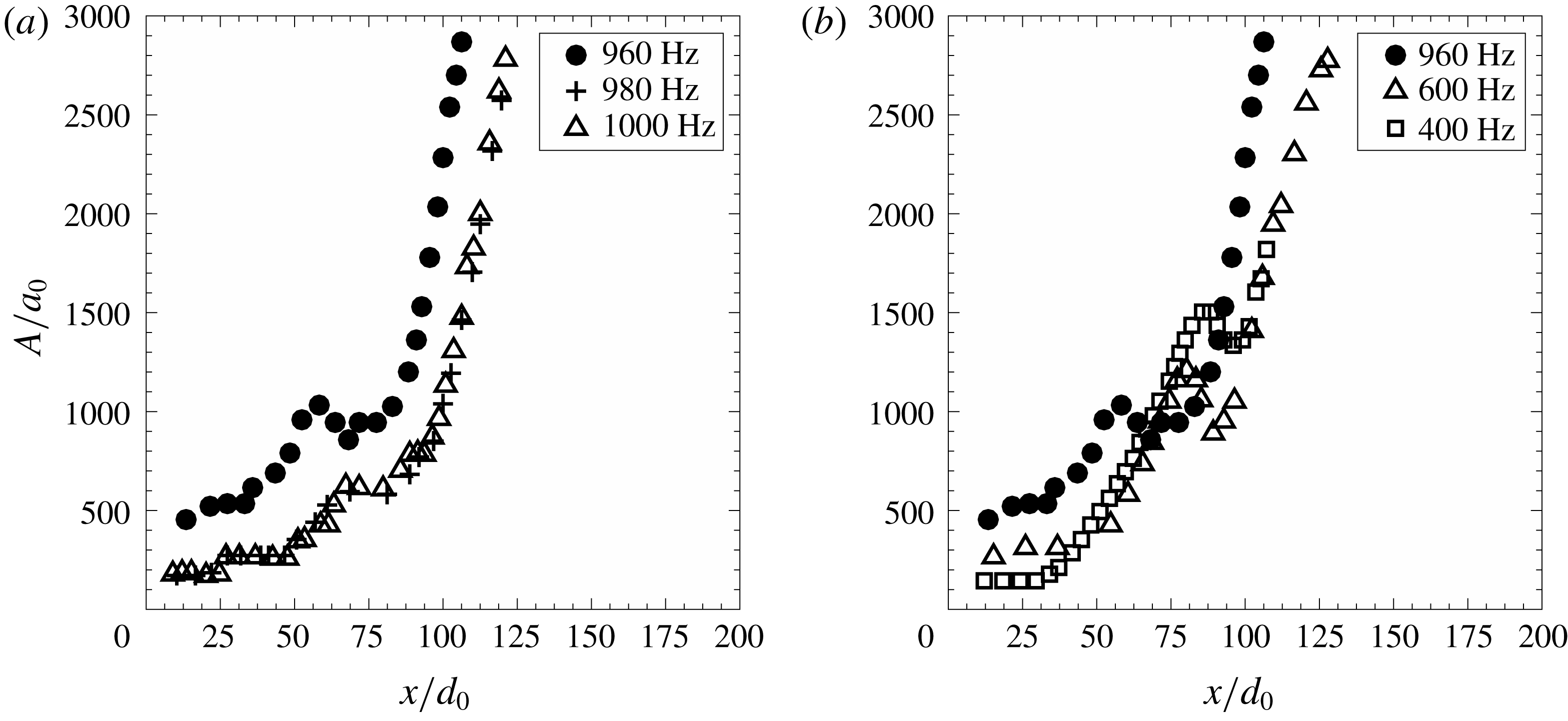
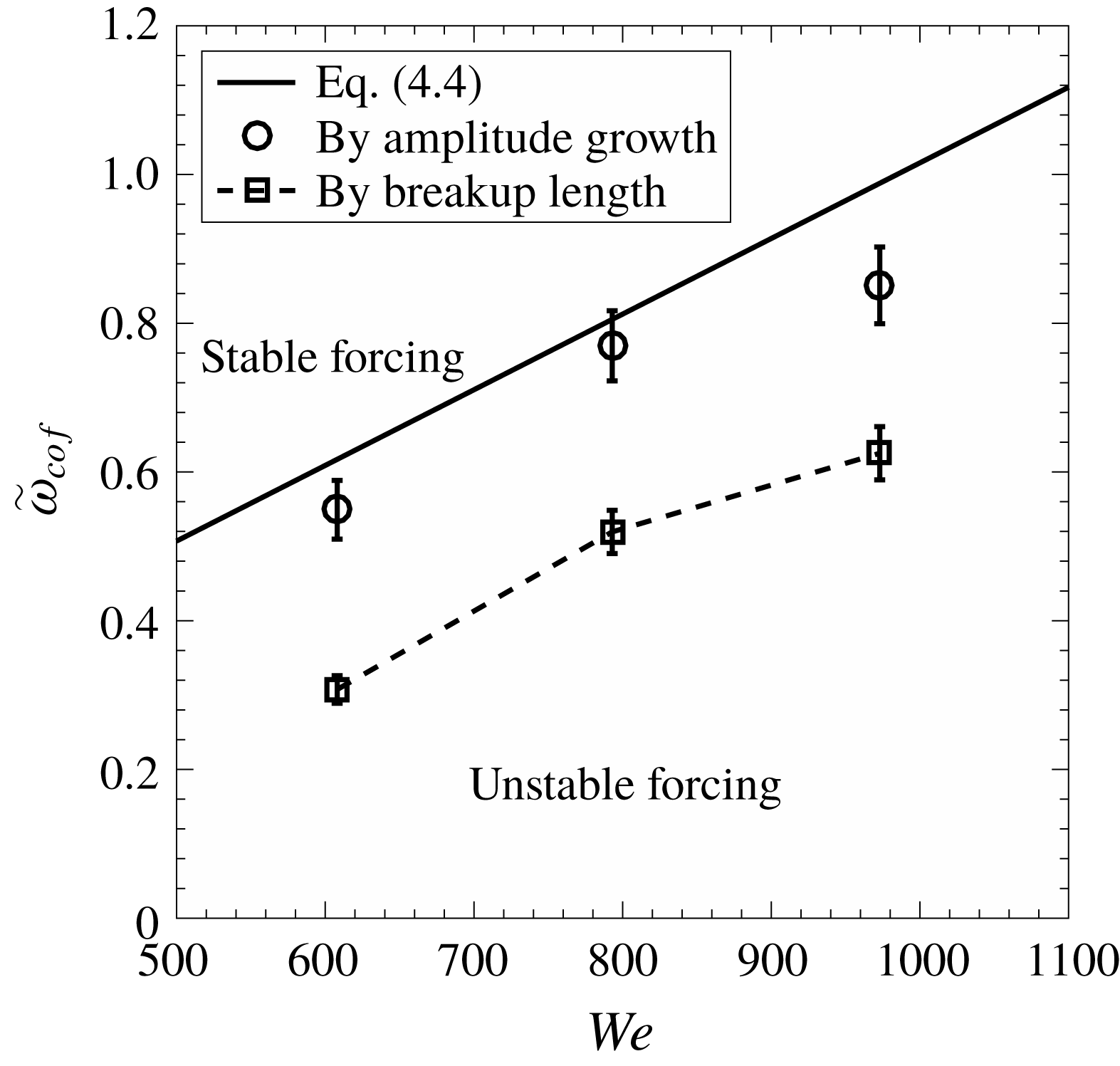
. Figure 20(a) shows the effect of higher frequencies and it may be noted that the sheet envelope is the same for frequencies of 980 and 1000 Hz. This means that the amplitude of the first antinode is almost the same for these frequencies and frequencies more than these. However, the rise in the amplitude may be noted for 960 Hz. The effect of forcing frequencies lower than 960 Hz is shown in figure 20(b). It may be observed that the amplitude of the first antinode increases successively as the frequency is reduced. This observation enables us to identify the cutoff frequency of 980 Hz corresponding to the Weber number of 973. The sheet is said to be stable for frequencies above 980 Hz, although the absolute amplitude increases spatially.
Experimental measurements of the sheet envelope at different forcing frequency used to find the cutoff frequency for
 $We=973$
. The onset of the instability of the sheet (unstable forcing) is when the amplitude of the first antinode starts increasing (in (a) for 960 Hz). (b) Forcing below the cutoff frequency.

Identification of the cutoff frequency essentially separates the regimes of stable and unstable forcing. Figure 21 shows the variation of the cutoff frequency in non-dimensional form with Weber number, and correspondingly the regions of stable and unstable forcing. It is interesting to note that the cutoff frequency predicted by linear theory (4.4) is in good agreement with the experimentally derived frequencies. A similar observation was reported by Bremond et al. (Reference Bremond, Clanet and Villermaux2007), where they perturbed the impingement point mechanically in a controlled manner to induce a pure sinuous mode on the sheet. The fact that a similar agreement is observed in the case of acoustic forcing imposed on the whole sheet emphasizes the importance of the linear theory. It is important at this point to draw attention to the cutoff frequency we have defined in the previous section based on the measurements of breakup length. It was defined as the frequency above which the breakup length does not show an appreciable (more than 5 %) variation. The cutoff frequencies based on the breakup length, also plotted in figure 21, show a similar trend qualitatively; however, they are lower than those predicted and the observed cutoff frequencies based on the amplitude growth. Physically, this means that, even though there is an increase in the peak amplitude, it is not sufficient enough to cause a significant change in the breakup length or the mean drop size (refer to figure 13). We may therefore define two cutoff frequencies associated with this phenomenon, viz. lower and higher. Above the lower cutoff frequency, the sheet characteristics saturate with no further significant change. The higher cutoff frequency saturates the wave growth in terms of the amplitude of the first antinode. Thus, there exists a region between the lower and higher cutoff frequencies where the forcing may be said to be metastable, which results in wave amplification without altering the atomization characteristics.
Variation of experimentally observed cutoff frequency and theoretical cutoff frequency based on wave amplitude with Weber number. The dashed line is the theoretical prediction of the cutoff frequency from (4.4). The circles and squares show the cutoff frequencies based on the amplitude growth and breakup length criteria, respectively.

4.2 Sheet envelope for stable and unstable forcing
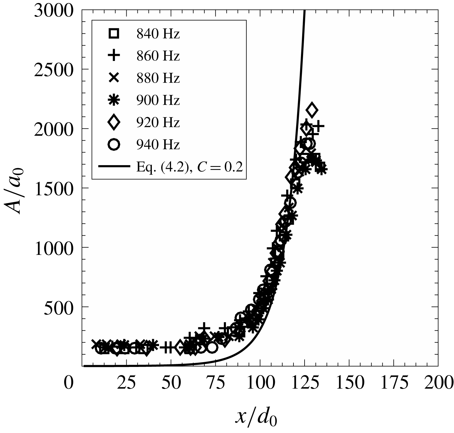
If the sheet is forced with a frequency that is greater than the cutoff frequency, then it is unaffected by such frequency and the amplification factor or gain will be the same as that of the unforced condition. To show this, we select
 $We=793$
, for which the cutoff frequency is 800 Hz. If the sheet is forced with frequencies greater than 800 Hz, then the amplification can be predicted by the exponent of maximum gain (4.2). Figure 22 shows the experimental sheet envelope for
 $We=793$
, for frequencies greater than the cutoff frequency and the gain or amplification factor for the natural mode (4.2) is shown by the solid line. Although the sheet is excited with the external frequency, it can be clearly observed that the gain (
 $A/a_{0}$
) is the same as that of the unforced condition. It can be concluded that, if the sheet is excited with a frequency greater than the cutoff frequency, then the natural mode only amplifies and the sheet is unaffected by the forcing.
Envelopes of an excited sheet for stable forcing frequencies (
 $We=793$
). The solid curve is the theoretical prediction of the maximum gain (4.2) in the unforced condition.

Now, we discuss the condition of unstable forcing, in which the sheet is excited with a frequency less than its cutoff frequency. As the sheet is excited with the external acoustic field with a certain frequency, we excite the spatially developing mode of the same frequency. The present problem is of spatial convective instability and hence the frequency is real and the wavenumber is imaginary. The spatial growth rate is given by the imaginary part of the wavenumber. For the long-wave approximation (
 $kh\ll 1$
), along with the thickness distribution given by
 $h=d^{2}/0.7r$
, equation (4.1) can be expressed as
 $$\begin{eqnarray}\displaystyle \left(1-\frac{1.4\tilde{x}}{We}\right)\tilde{k}^{3}-2\tilde{\unicode[STIX]{x1D714}}_{e}\tilde{k}^{2}+\tilde{\unicode[STIX]{x1D714}}_{e}^{2}\tilde{k}+1.4\unicode[STIX]{x1D6FC}\tilde{x}\tilde{\unicode[STIX]{x1D714}}_{e}^{2}=0. & & \displaystyle\end{eqnarray}$$
Here,
 $\tilde{\unicode[STIX]{x1D714}}_{e}$
is the non-dimensional excitation frequency. The gain or amplification factor increases spatially and after the critical sheet length it remains constant. The maximum gain is given by Bremond et al. (Reference Bremond, Clanet and Villermaux2007)
 $$\begin{eqnarray}\displaystyle G_{m}=\int _{\tilde{r}_{0}}^{\tilde{x}_{c}}\tilde{\unicode[STIX]{x1D714}}_{ei}\,\frac{\text{d}\tilde{x}}{\tilde{c}_{g}}. & & \displaystyle\end{eqnarray}$$
From the two solutions (positive and negative) of (4.1) and following a similar approach used for the mechanically vibrated liquid sheet by Bremond et al. (Reference Bremond, Clanet and Villermaux2007), the sheet surface deflection amplitude is given by
 $$\begin{eqnarray}\displaystyle a(\tilde{x},\tilde{t})=a_{1}\exp [G(\tilde{x})]+a_{2}\exp [-G(\tilde{x})]\sin (\tilde{\unicode[STIX]{x1D714}}_{e},\tilde{t}). & & \displaystyle\end{eqnarray}$$
Here,
 $a_{1}$
and
 $a_{2}$
are the initial amplitude of the two waves. The initial deflection is equal to the particle displacement (
 $a_{0}$
) given by (2.3). Therefore,
 $a_{2}=a_{0}-a_{1}$
. The wave amplitude normalized by
 $a_{0}$
is
 $$\begin{eqnarray}\displaystyle \frac{A(\tilde{x})}{a_{0}}=\frac{a_{1}}{a_{0}}\exp [G(\tilde{x})]+\left(1-\frac{a_{1}}{a_{0}}\right)\exp [-G(\tilde{x})]. & & \displaystyle\end{eqnarray}$$
The maximum amplitude defined by maximum gain (
 $G_{m}$
) is
 $$\begin{eqnarray}\displaystyle \frac{A_{m}}{a_{0}}=\frac{a_{1}}{a_{0}}\exp (G_{m})+\left(1-\frac{a_{1}}{a_{0}}\right)\exp (-G_{m}). & & \displaystyle\end{eqnarray}$$
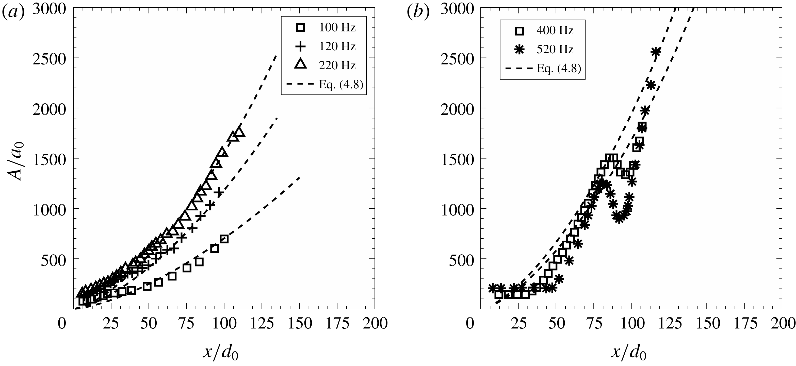
Now, the sheet is excited below its cutoff frequency. Figure 23 shows the experimentally measured sheet envelopes and those (dashed lines) predicted by (4.8). Depending on the excitation frequency, the unstable sheet disintegrates in two ways. Either the sheet envelope amplitude continuously diverges until the sheet breaks (figure 23 a) or the envelope amplitude grows in an oscillatory fashion, forming multiple antinodes. The sheet envelopes for both cases are shown in figure 23. The predicted envelope for different frequencies is obtained from (4.8) and is compared with experimental envelopes in figure 23. It may be seen from figure 23 that there is a good match between the experiments and the theory.
Envelopes of an excited sheet for unstable forcing frequencies (
 $We=973$
). The dashed curve is the theoretical prediction envelope from (4.8) for unstable forcing frequencies. At lower frequencies, the wave amplitude diverges (a) and for higher frequencies the amplitude of the first antinode increases before diverging (b).

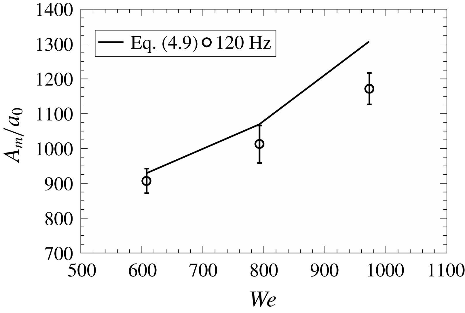
Maximum amplification shown for different Weber numbers at 120 Hz, 109 dB. The solid line shows the amplitude predicted by (4.9).

Figure 24 shows the comparison between the maximum wave amplitude for several Weber numbers at 120 Hz, 109 dB. The amplification is higher for higher Weber number for similar excitation condition. The high jet velocity leads to high and fast growth in amplitude. The experimentally measured maximum amplitude agrees satisfactorily with the predicted one for different Weber numbers. Thus, the present analysis shows that the external acoustic forcing essentially augments the growth of the sinuous waves responsible for the sheet breakup without affecting the primary instability mechanisms; and the whole phenomenon can be described with the help of the linear theory of Squire (Reference Squire1953).
5 Conclusion
The objective of the present study is to investigate the breakup of a smooth laminar liquid sheet formed by the oblique impact of two jets in the presence of external acoustic forcing. Though the effect of external perturbations, either mechanical or acoustic, on various sheet configurations has been studied so far in various contexts, the present investigations reveal a number of new insights in the theory of sheet breakup. The experimental observations show that a liquid sheet exposed to an acoustic field fragments in a similar fashion to an undulating liquid sheet under the influence of sinuous waves emanating from the impingement point. The wave growth makes the sheet flap like a flag at lower frequencies and the peak amplitude of flapping comes down with increase in the frequency. The sheet characteristics, like the breakup length and the mean drop size, reduce significantly for forcing frequencies below a certain critical frequency and this critical frequency increases with Weber number.
The application of linear theory (Squire’s theory) to the above problem provides a new critical frequency above which the growth of sinuous waves saturates and it is termed the higher cutoff frequency since its value is greater than the cutoff frequency based on the breakup length variation. The higher cutoff frequency derived from the linear theory matches well with experimentally obtained values. Interesting inferences can be deduced from the two cutoff frequencies. The variation in breakup characteristics ceases above the lower cutoff frequency and it is more critical for practical combustors. Between the lower and higher cutoff frequencies, the amplitude of waves shows growth without affecting the atomization characteristics. Beyond the upper cutoff frequency, the amplitude growth also ceases and the natural breakup is observed even in the presence of forcing. This shows that the atomization characteristics are sensitive to the absolute critical wave amplitude, which is independent of the Weber number. The droplet statistics is sensitive to forcing frequencies smaller than the lower cutoff frequency. However, it is remarkable to see that the drop size distribution is well described by the Gamma distribution when normalized by the mean drop diameter and it is insensitive to the forcing condition.
Supplementary movies
Supplementary movies are available at https://doi.org/10.1017/jfm.2019.732.
Appendix A. Effect of acoustic field at very low Weber number
A.1 Sheet regimes and characterization
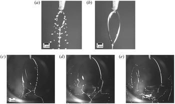
Figure 25 shows the different sheet regimes observed in the present study. For low jet velocity, the two jets just impinge on each other and form a tiny sheet. As the jet velocity is increased, the sheet starts spreading and grows in size. With increase in the jet velocity, the sheet rim becomes unstable, due to small perturbations, leading to the sheet rim breakup. The unstable rim sheds droplets periodically and hence such a sheet structure is called periodic atomization, as shown in figure 25(a). The droplet shedding due to the rim instability results in three droplet trails below the leaf-like sheet, which resemble fishbones, and hence the periodic sheet regime is also referred to as the fishbone structure. Further increase in the jet velocity leads to the disappearance of droplet trails and then the sheet suddenly converts into a smooth sheet with fluid chains as shown in figure 25(b). The smooth sheets are orthogonally connected to each other, forming a chain. Such a sheet regime is called the fluid chain regime. At higher flow rate, the sheet breaks at the bottom before the formation of the second sheet as shown in figure 25(c). The upper portion of the sheet remains smooth and laminar. We classified this sheet regime into smooth or laminar sheet regime.
Sheet regimes for glycerol–water mixture: (a) periodic atomization (fishbone),
 $We=2$
; (b) fluid chain,
 $We=10$
; and (c–e) smooth or laminar sheet regime,
 $We=608$
(c),
 $We=793$
(d) and
 $We=973$
(e).

A.2 Acoustic forcing on the liquid sheet at very low Weber number
We classify the periodic atomization (
 $We=2$
) regime and the fluid chain regime (
 $We=10$
) in the very-low-Weber-number range (
 $We<100$
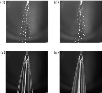
). Figure 26 shows the effect of acoustic excitation on the sheet structure for the periodic breakup regime. The sheet shape and size in the presence of excitation remain unaltered. Only the regular droplet trails below the sheet gets affected. From figure 26(a) and (b) it can be clearly observed that the droplets shedding from the sheet rim show irregular trails in the presence of acoustics. The time-averaged droplet trajectories created by overlapping the sheet images (sequence of 500) are shown in figure 26(c) and (d) without and with acoustic excitation, respectively. The droplet trajectories without excitation are well defined, but for the excited condition the irregular droplet movement leads to diffused droplet trajectories (figure 26
d). The acoustic excitation only affects the rim instability in the periodic atomization regime.
Effect of acoustic forcing on the periodic atomization regime (
 $We=2$
): (a) instantaneous image of unexcited sheet; (b) acoustically excited sheet (120 Hz 107 dB) (c,d) the sheet envelopes showing the droplet trajectories for unexcited (c) and excited (d) conditions.

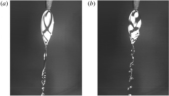
Effect of excitation on the fluid chain regime: (a)
 $We=10$
unexcited, and (b)
 $We=10$
, 120 Hz, 107 dB. See also supplementary movie 7.

Figure 27 shows the effect of acoustic field on the fluid chain regime. The position of the light source is adjusted in such a way that the sheet illumination shows the bright sheet surface. The acoustic excitation perturbs the liquid sheet, and the symmetric wave pattern (two standing waves crossing each other), which is a characteristic of such low-
 $We$
sheets, gets disordered (figure 27
b). The fluid chain structure below the sheet breaks due to the excitation. Apart from this, there are no significant changes in the sheet characteristics due to the acoustic excitation for the fluid chain regime. The acoustic excitation of the sheet regimes at low Weber number shows that there is no significant effect of acoustic field on the sheet characteristics (breakup length, width, etc.) as well as on the sheet disintegration. The main reason for this is that at lower Weber numbers the surface tension force dominates the inertia force and the acoustic perturbations. Hence, the studies at lower Weber numbers are not presented in detail.