1. Introduction
This research is driven by the study of boundary layer transition in converging–diverging sonic nozzles employed in industrial applications as flow meters. The application of a quasi-one-dimensional theory provides an accurate prediction of the total mass flow rate, with errors of the order of
 $0.5\,\%$
. Discrepancies are attributed to multidimensional effects, such as non-uniformity within the core flow and the formation of boundary layers. At the nozzle throat, the sonic boundary layer is influenced by a favourable pressure gradient and a centrifugal force resulting from the curvature of the nozzle wall. Although the boundary layer displacement thickness at the nozzle throat is minimal, it affects the mass flow rate by reducing the effective sonic area and is typically incorporated into mass-flow-rate models as a discharge coefficient (
 $C_d$
).
The pioneering theoretical studies of Hall (Reference Hall1959) and Stratford (Reference Stratford1964) demonstrated, using an integral method, that the discharge coefficient approaches unity as the Reynolds number increases, due to the thinning of the boundary layer. However, this trend is non-monotonic, and the discharge coefficient may notably decrease during transition, attributed to the formation of a thicker turbulent boundary layer. A representative nozzle geometry utilised in industrial settings, depicted in figure 1, maintains a ratio of convergent radius to throat diameter
 $R/D = 2$
, and was designed based on the recommendations of Stratford (Reference Stratford1964) to minimise variations in the discharge coefficient induced by transition. Subsequent experimental evaluations by Szaniszlo (Reference Szaniszlo1975), among others, revealed that, despite the recommended nozzle geometry, a decline in the discharge coefficient is discernible during calibration.
In an attempt to minimise the drop in discharge coefficient, Ishibashi (Reference Ishibashi2015) tested multiple nozzle geometries. The ratio
 $R/D$
was modified to obtain a smooth
 $C_d$
curve over the transitional regime and it was found that the transition Reynolds number
 ${\textit{Re}}_t^{tr}$
depends on the nozzle geometry. It is also found that modifying the upstream section of the nozzle by introducing an obstacle impacts
 ${\textit{Re}}_t^{tr}$
. The roughness effect on transition was investigated by Demetriades (Reference Demetriades1981) for a nozzle with large
 $R/D$
. It was found there that transition can be correlated to roughness with an appropriate Reynolds number on the basis of the roughness height and the boundary layer momentum thickness. That study also showed that below a given roughness height, transition occurs at a fixed
 ${\textit{Re}}_t^{tr}$
. In that case, it was suggested that transition is triggered by free stream disturbances present in the facility rather than the roughness of the nozzle. More recently, from a direct numerical simulation database for isolated roughness-induced transition, Bernardini et al. (Reference Bernardini, Pirozzoli, Orlandi and Lele2014) suggested values for critical Reynolds number with multiple roughness shapes on a flat-plate boundary layer that can be used as an approximate reference for the present case, considering that the very low curvature investigated should have small effects on the critical Reynolds number values.
A prevalent methodology for examining boundary layer transition involves the analysis of modal growth of infinitesimal disturbances within a linearised base flow. In the converging section of a nozzle, the boundary layer spans subsonic to transonic regimes. For a flat plate in a transonic regime, the transition is predominantly influenced by the Tollmien–Schlichting (TS) wave. At sonic velocities, planar two-dimensional (2-D) and three-dimensional waves are comparably unstable (Mack Reference Mack1984; Özgen & Kircali Reference Özgen and Kircali2008; Ren & Fu Reference Ren and Fu2014), although this instability is mitigated by the presence of a favourable pressure gradient (Mack Reference Mack1984; Masad & Zurigat Reference Masad and Zurigat1994), which is applicable to the present investigation. This phenomenon has been extensively studied on blunt cones at hypersonic speeds, where the region proximal to the stagnation point exhibits characteristics analogous to the current study: subsonic speed, curvature and pressure gradient. Despite the presence of a favourable pressure gradient, it has been observed that transition might still occur in the blunt region.
These insights have prompted further investigation into transient growth as a potential mechanism for transition. Research into compressible transient growth, conducted by Hanifi, Schmid & Henningson (Reference Hanifi, Schmid and Henningson1996) using a temporal framework for flat-plate boundary layers, revealed that streamwise vortices can induce the formation of streaks of high and low streamwise velocity through the lift-up mechanism articulated by Landahl (Reference Landahl1980) for incompressible shear flows. A parabolised spatial transient-growth formulation employed by Tumin & Reshotko (Reference Tumin and Reshotko2001) indicated that a favourable pressure gradient diminishes the maximum gain produced by steady streaks in flat-plate boundary layers. The effects of curvature were subsequently examined by Tumin & Reshotko (Reference Tumin and Reshotko2004) and Zuccher, Tumin & Reshotko (Reference Zuccher, Tumin and Reshotko2006), revealing that convex surfaces attenuate the maximum gain for steady disturbances. Moreover, the investigations of unsteady perturbations at a single frequency by Tumin & Reshotko (Reference Tumin and Reshotko2001) demonstrated that the gains of unsteady streaks are lesser than those of steady streaks. A spatial transient growth analysis concerning convex surfaces for incompressible boundary layers, as conducted in Karp & Hack (Reference Karp and Hack2018), reports that the optimal streaks are unsteady, with their frequencies dependent on the surface curvature and Reynolds number.
The combined experimental examination and linear stability analysis of unsteady disturbances in transonic nozzle flow, characterised by a concave curvature and compressibility, is scarcely addressed in the literature. To our knowledge, non-modal, linear-analysis methodologies have not been employed to tackle this issue. Consequently, this paper seeks to elucidate the transition mechanism in mass-flow nozzles both experimentally and theoretically. An experimental study is undertaken to discern the influence of (i) nozzle surface roughness, (ii) radius of curvature of the nozzle and (iii) the level of free stream turbulence on transition. The experimental observations are subsequently modelled using linear stability analysis. The structure of the work is as follows: the experimental set-up is described in § 2, and the results are analysed in § 3. The modal stability of the flow is examined in § 4, where an analysis of the eigenvalue spectrum is conducted in preparation for the spatial non-modal transient growth model discussed in § 5. Transient growth analysis is employed to model the transition using the N-factor and is compared with the experimental data in § 6. Further inquiry into the origins of disturbances is explored in § 7. The conclusions and future directions of the study are summarised in § 8.
The ISO 9300 toroidal nozzle standard for mass flow rate measurements.

2. Experimental set-up
2.1. Wind tunnel characteristics
The experimental investigations are conducted using the S150 blowdown facility at the PPRIME Institute in Poitiers, whose sketch is provided in figure 2. The facility operates at a total pressure ranging from 1 to 40 bar, with flow rates reaching up to 5 kg s−1. The working fluid, dry air, is initially stored in a 50 m
 $^{3}$
reservoir at 200 bar. It is subsequently expanded to a pressure between 1 and 40 bar via a dome regulator controlled by a proportional integral–derivative system, ensuring pressure stability. Due to the Joule–Thomson effect, the air experiences cooling during expansion and is subsequently reheated using a heat exchanger composed of eight tons of nickel spheres, preheated to the target total temperature. The heater temperature can be adjusted within the range of 295–330 K, with a temperature variation of less than 0.2 K over a 30 s test duration. Following passage through the test section, the air is directed into an outlet silencer at atmospheric pressure.
Sketch of the high-pressure blowdown wind tunnel.

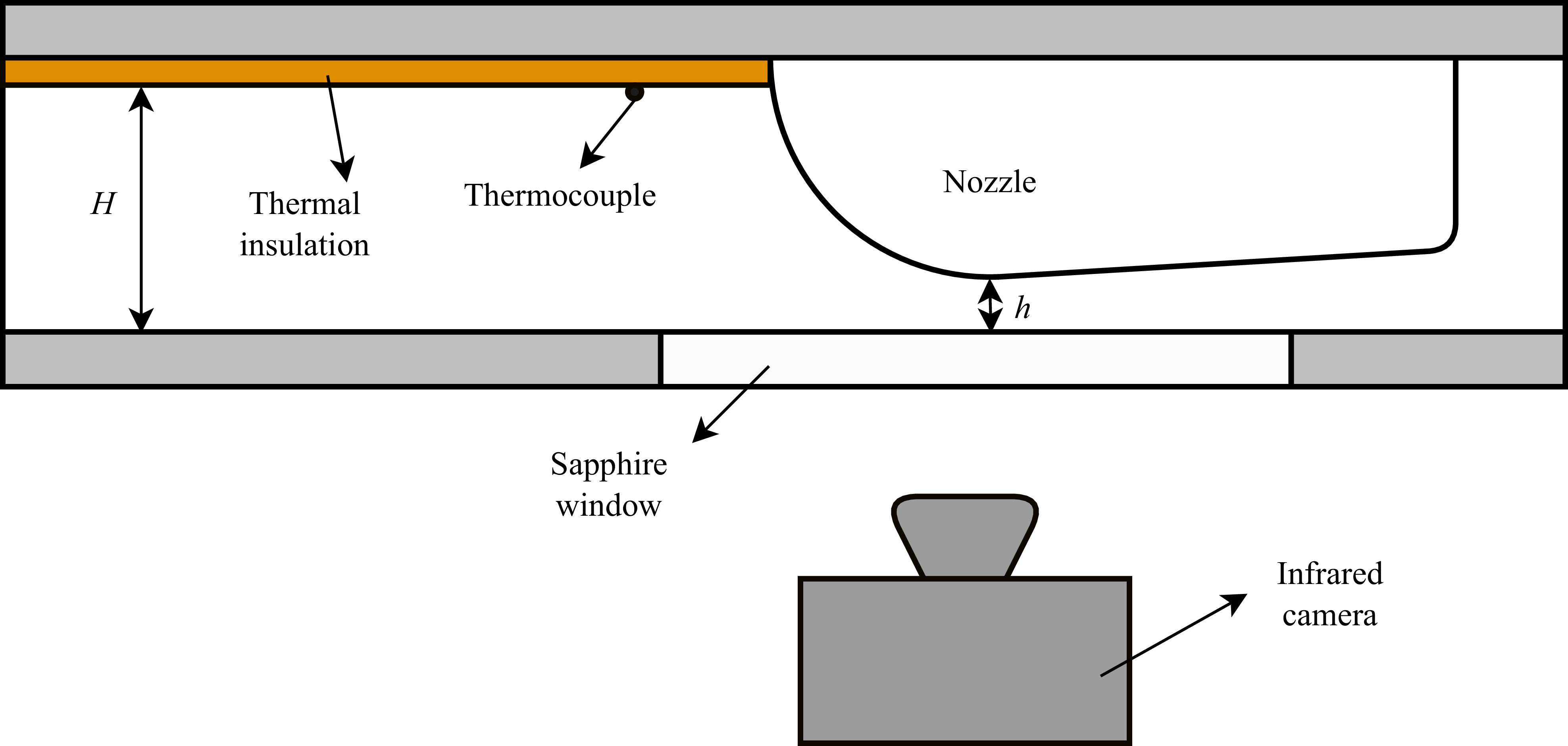
Due to accessibility constraints imposed by measurement techniques, the industrial configuration with axisymmetric nozzles (depicted in figure 1) was adapted to a planar nozzle configuration, as shown in figure 3. Since the boundary layer is extremely thin compared with any other geometrical dimension of the problem, it is conjectured that the planar nozzle remains a relevant case to study. It allows direct experimental investigation of the near-wall flow behaviour while allowing the reproduction of the dominant mechanisms that drive the transition process. To facilitate optical access, a sapphire window is flush-mounted with the wall on the plane of symmetry.
Sketch of the test section in planar configuration.

The total pressure in the settling chamber is measured using a Keller 33XX series pressure transducer with a measurement range of 0–60 bar, providing pressure data with an uncertainty of
 $\pm 60$
mbar. The temperature is recorded upstream of the nozzle using a
 $0.25$
mm-diameter thermocouple, calibrated against a PT100 probe, with an associated uncertainty of
 $\pm 0.2$
K. The rectangular section upstream of the nozzle has a width of
 $W = 60$
mm and a height of
 $H = 25$
mm. Three different nozzles were employed, featuring throat heights of
 $h = [2.1, 2.5, 5]$
mm. The variation in throat height enables modulation of the contraction ratio, defined as
 ${\textit{CR}} = H/h$
, thereby influencing the turbulence intensity at the nozzle throat. Ideally, the investigation of boundary layer transition should be conducted using Reynolds numbers based on the displacement thickness of the boundary layer. However, given that the boundary layer thickness is estimated to be of the order of
 $30\,{\unicode{x03BC}}\text{m}$
, direct measurement is impractical. Consequently, the Reynolds number is defined using a reference length based on the nozzle throat height
 $D$
,
 \begin{equation} {\textit{Re}}_t = \dfrac {\rho ^* u^* D}{\mu _0}, \end{equation}
where
 $\rho ^*$
is the density at the nozzle throat,
 $u^*$
is the velocity at the nozzle throat and
 $\mu _0$
is the stagnation viscosity obtained from Sutherland’s formula and the subscript
 $t$
stands for throat. To remain consistent with the literature, the Reynolds number is here calculated with the throat height
 $D = 2h$
, treating the wind tunnel floor containing the window as a plane of symmetry. The flow temperature at the nozzle wall being close to the total temperature, the stagnation viscosity is used rather than the free stream one to better represent the flow conditions within the boundary layer. The density and viscosity are estimated based on the pressure and temperature measurements. In the test section, the flow upstream of the nozzle is subsonic,
 $M=0.117$
and
 $M\leqslant 0.06$
for nozzles with a throat height
 $h=5\,\rm mm$
and
 $h\leqslant 2.5\,\rm mm$
, respectively. When passing through the nozzle, the flow accelerates to
 $M=1$
at the throat, producing a strong favourable pressure gradient. The flow continues to accelerate in the divergent section, until approximately
 $M = 2$
before being guided into the silencer.
2.2. Characteristics of investigated nozzles
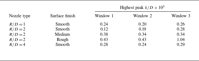
To study the boundary layer transition in the nozzles, the parameter space is made of three radii of curvature, three roughness levels and two contraction ratios. The parametric study was designed to independently investigate the effects of geometry, roughness and free stream turbulence intensity on the boundary layer transition. The characteristics of the nozzles are summarised in table 1.
Nozzles characteristics. The nozzle naming refers to R, inlet radius; C, contraction ratio; the final letters [S, M, R] stand for smooth, medium, rough surface finish.

In order to allow the investigation of several geometries and surface states, the nozzles are made of polylactic (PLA) and 3D-printed by a fusion deposit material process. This choice of material and manufacturing process is in line with the context of transition measurement: the low thermal conductivity of the plastic is suitable to approach the adiabatic conditions and the material allows the required surface finish to be obtained while keeping acceptable infrared thermal radiation properties (see § 2.4). The three-dimensional printing process induces surface waviness due to the layer-by-layer printing process. These ripples have a depth of approximately
 $75\,{\unicode{x03BC}}\textrm{m}$
. To obtain the desired surface finish, the parts are sanded with coarse sandpaper, and then finished with fine sandpaper according to the different surface finishes desired.
The surface roughness is characterised on a TalySurf CCI 6000 optical interferometer. The resolution of the wall-normal direction is
 $0.01 \; \rm nm$
and the lateral resolution is
 $0.35\, {\unicode{x03BC}} \rm m$
. To assess the nozzle roughness, each one is measured at the throat in three lateral positions, with a measurement area of
 $0.36 \times 0.36 \; \rm mm^2$
. The roughness shown in table 1 is the average of the three measurements. The roughness is defined using the arithmetic roughness criterion
 \begin{equation} \textit{Ra} = \dfrac {1}{l} \int _0^l |\zeta ^*(z^*)| {\rm d}z^*, \end{equation}
where
 $\zeta ^*(z^*)$
is the variation of the surface profile around its mean value and
 $l$
is the length of the measured segment. The reference roughness is dictated by the standard ISO 9300:2005 2005 (E), describing the characteristics of industrial flow meter which requires that nozzles have a surface finish better than
 ${\textit{Ra}} \lt 15 \times10^{-6} D$
. Within the group of nozzles studied, only nozzles with a ‘smooth’ finish with a
 $h =5\,\rm mm$
throat meet this criterion.
2.3. Turbulence level
The wind tunnel turbulence intensity is measured by placing a single
 $5\,{\unicode{x03BC}} \rm m$
hot wire in the centre of test section upstream of the nozzle, in a region with no pressure gradient. The presence of the hot wire and its support introduces disturbances downstream of the flow, so the turbulence intensity and transition measurements are performed separately to avoid any contamination in the transition data. The velocity samples are obtained using a Constant Temperature Anemometry unit, clocked at a frequency of
 $40 \; \rm kHz$
for an acquisition time of
 $30 \; \rm s$
.
The hot wire calibration is performed in situ by recording the output voltage for varying total pressure of the wind tunnel. For each total pressure step, the density is indirectly measured using pressure and temperature sensors. The velocity is calculated from temperature measurements and the contraction ratio
 $H/h$
, via the isentropic relations of compressible flow. The signal recorded over all pressure steps is giving the calibration curve
 \begin{equation} \bar {V} = f_{\textit{cal}}(\bar {\rho } \bar {U}), \end{equation}
where
 $V$
is the tension,
 $U$
is the velocity,
 $\rho$
is the density and the overbar denotes the time average at constant total pressure. Since the flow at the hot wire location is at low Mach numbers, typically
 $M \approx 0.1$
, it is considered incompressible for all total pressures. Velocity samples are obtained using the following formulae:
 \begin{equation} U'(t) = \dfrac {f_{\textit{cal}}^{-1}(V(t))}{\bar {\rho }}-\bar {U}, \end{equation}
where
 $U'$
is the fluctuating velocity. Finally, the turbulence intensity is obtained with
 \begin{equation} \textit{Tu} = \dfrac {\sqrt {\overline {U^{{\prime }^2}}}}{\bar {U}}, \end{equation}
and is calculated for each total pressure set. The evolution of the turbulence intensity as a function of Reynolds number for the two contraction ratios studied is shown in figure 4. The turbulence intensity increases with the Reynolds number in both cases, but that of the
 ${\textit{CR}} = 10$
increases more rapidly, from
 ${\textit{Tu}} \approx 0.4\,\%$
to
 ${\textit{Tu}} \approx 1\,\%$
over the range
 ${\textit{Re}}_t \approx [0.1 {-} 2]\times10^6$
. This variation of
 ${\textit{Tu}}$
can influence the transition and should be kept in mind when analysing the experimental results.
Turbulence intensity as function of Reynolds number for the two contraction ratios
 ${\textit{CR}} = 10$
and
 ${\textit{CR}} = 5$
.

However, one must note that these turbulence intensity values are not representative of the free stream turbulence at the nozzle throat. Indeed, when the flow is accelerated to sonic velocities, the turbulence level will change. In general, a higher contraction ratio tends to decrease the turbulence intensity more strongly (Tsugé Reference Tsugé1984). Thus, it is possible that the turbulence level at the nozzle throat is lower for higher contraction ratios, contrary to what the figure 4 suggests. Although it does not provide quantitative information about the
 ${\textit{Tu}}$
at the throat, this data is useful to examine qualitatively the effect of
 ${\textit{Tu}}$
on the transition.
2.4. Transition detection methodology
One of the characteristic features of flow metering nozzles is the strong acceleration of the flow along the wall. This favourable pressure gradient leads to a thin boundary layer. Based on the observation of Ishibashi (Reference Ishibashi2015) and an adapted model (see § 4.1), the boundary layer thickness is estimated at
 $\delta \approx 33\,{\unicode{x03BC}} \rm m$
when the transition occurs for the
 $R/D =2$
and
 $h = 5 \; \rm mm$
nozzle. In the most extreme case, i.e.
 $R/D =2.4$
and
 $h=2.1 \; \rm mm$
, the boundary layer thickness is estimated to be
 $\delta \approx 20\,{\unicode{x03BC}} \rm m$
just before the transition. In addition to the small size of boundary layer, the measurement is made difficult due to the wall curvature and the transonic flow regime, which is sensitive to small geometry variations.
To perform the measurement in a non-intrusive manner, the boundary layer transition is detected by measurement of the nozzle wall temperature through infrared imaging. When the flow is accelerated to sonic velocities, the adiabatic recovery temperature at the wall
 $T_w^{ad}$
is given by
 \begin{equation} T_w^{ad} = T_\infty \left(1+{\Re}\dfrac {\gamma -1}{2} M_\infty ^2\right)\!, \end{equation}
where
 $M_\infty$
is the free stream Mach number and
 ${\Re}$
is the recovery coefficient. During the tests, the temperature is kept constant and the Mach number is fixed by the nozzle geometry. The recovery coefficient can vary depending on the state of the boundary layer,
 $\Re \approx 0.84$
for laminar boundary layers and
 $\Re \approx 0.90$
for turbulent ones are commonly reported values (Tropea, Yarin & Foss Reference Tropea, Yarin and Foss2007, p. 545–546). Under our experimental conditions with a total temperature
 $T_0 = 300 \; K$
and
 $M=1$
at the nozzle throat, a maximal difference
 $\Delta T$
of
 $3\,\rm K$
can be expected between a laminar and a turbulent boundary layer. Due to unperfect thermal insulation and progressive wall cooling during the experiment, this variation will be even lower in practice. To measure this temperature variation, a FLIR SC7200 thermal camera is used for its low noise equivalent temperature difference of
 $25 \; \rm mK$
.
The detection of the transition by infrared measurement constrains the choice of wall materials. The thermal radiation
 $\dot {f}$
used to measure the temperature is expressed as
 \begin{equation} \dot {f} = \sigma \varepsilon T^4, \end{equation}
where
 $\sigma = 5.670 \times10^{-8} \;\rm W\,m^{-2}\,K^{-4}$
is the Stefan–Boltzmann constant,
 $\varepsilon$
is the emissivity of the surface and
 $T$
its temperature. The emissivity
 $\varepsilon$
varies between 0 and 1 depending on the material, the surface roughness and viewing angle. In general, metallic surfaces have a low emissivity, of the order of
 $\varepsilon \approx 0.1$
, and smoother surfaces have lower emissivities than rougher ones. In addition, the emissivity of a surface decreases sharply for high viewing angles. For these reasons we machined our nozzles using PLA, which, having high emissivity, allows for thermal measurements of smooth surfaces. Optical measurements of the nozzle surface are made through a window on the opposite side of the nozzle (see figure 3). A sapphire window was used as to maximise the transmittance in the infrared wavelengths.
2.5. Data acquisition and processing procedure
The infrared image of the nozzle surface shows reflections due to the sapphire window and the polished nozzle surface, that are removed by subtracting a reference image, taken at rest, before each test.
Data for different Reynolds numbers are acquired by varying the wind tunnel total pressure in increments of
 $0.5$
bar. For each pressure step, 10 infrared images, synchronised with stagnation temperature and pressure measurements, are acquired. The data are then time-averaged and used to determine the Reynolds number and the boundary layer state.
3. Experimental results
3.1. Transition criterion
In order to describe the experimental evaluation of the transition Reynolds number, a representative wall temperature at the nozzle throat is plotted as a function of
 ${\textit{Re}}_t$
in figure 5. The temperature values correspond to spanwise-averaged measurements taken at the streamwise location of the nozzle throat. As observed, the temperature exhibits a non-monotonic dependence on
 ${\textit{Re}}_t$
. Initially, the temperature decreases to a minimum value, followed by an increase to a maximum, after which it decreases again.
In an ideal adiabatic framework, the wall temperature is not expected to vary with Reynolds number, except during the transition from a laminar to a turbulent boundary layer. In perfectly adiabatic conditions, this local average temperature profile would rather exhibit some plateau levels before and after the transition
 ${\textit{Re}}_t$
. Therefore, the observed temperature variations before the minimum and after the maximum are attributed to the imperfect adiabatic nature of the experimental walls. This imperfection introduces
 ${\textit{Re}}_t$
-dependent heat transfer effects, as higher
 ${\textit{Re}}_t$
leads to a thinner boundary layer, increased temperature gradients near the wall, and consequently, greater heat loss.
Despite these non-ideal adiabatic conditions, the significant temperature rise observed in the temperature profile can only be associated with the transition to turbulence. This confirms that the experimental set-up effectively captures the boundary layer transition process.
Wall temperature at the nozzle throat as function of Reynolds number for the
 $R/D = 2$
,
 ${\textit{CR}}=5$
, smooth finish nozzle.

In the Reynolds number range with a transitional boundary layer, between
 ${\textit{Re}}_t \approx 0.4 \times 10^6$
and
 ${\textit{Re}}_t \approx 1 \times 10^6$
, the temperature is between that of a laminar and that of a turbulent flow. As the Reynolds number increases, the increase in temperature reflects the increased occurrence of the turbulent events, until a completely turbulent boundary layer is reached. It was checked that the fully turbulent Re is independent of the spanwise location considered in the nozzle and that it is not affected by remaining optical disturbances (reflection of the camera lens, illumination defaults, etc.).
In the following, we retain the Reynolds numbers at which the minimum and the maximum temperatures are observed, corresponding to the beginning and to the end of the transition, respectively.
3.2. Effect of surface roughness
The surface roughness effect is studied by comparing the results from nozzles of various wall surface roughness R2C5S, R2C5M and R2C5R, whose contour is shown in figure 6. The infrared measurements were performed between
 ${\textit{Re}}_t = 0.15\times 10^6$
and
 ${\textit{Re}}_t = 1.7\times 10^6$
. As already mentioned, the temperature fields were averaged in the transverse direction and the temperature minima and maxima were extracted for various longitudinal positions.
Normalised contour of the R2C5 nozzle.

The transition results for the different positions are presented in figure 7. In the region under consideration, between
 $x/D = -1$
and
 $x/D = 0.9$
, it is observed that the boundary layer is initially laminar up to
 ${\textit{Re}}_t \approx 0.4 \times 10^6$
, then becomes transitional almost simultaneously throughout the entire region. In the divergent section of the nozzle (
 $x/D \gt 0$
), the transition starts at slightly lower Reynolds numbers, around
 ${\textit{Re}}_t \approx 0.35 \times 10^6$
. The Reynolds number at which the boundary layer becomes fully turbulent varies depending on the position within the nozzle. The boundary layer first becomes turbulent at the nozzle exit, and then the transition front gradually moves upstream as the Reynolds number increases.
Transition map in R2C5 nozzles for different roughness levels: circles (
 $\bigcirc$
), R2C5S; cross (
 $\times$
), R2C5M; diamonds (
 $\diamondsuit$
), R2C5R; green, yellow and oranges zones correspond to laminar, transitional and turbulent boundary layer states, respectively; solid/dashed lines indicate the locations where the flow starts/completes transition.

Overall, the transition dynamics are similar for the three levels of roughness, yielding very comparable results in terms of transition behaviour. The only notable difference arises from the roughest nozzle, R2C5R, for which the fully turbulent regime appears to be reached significantly earlier than for the other nozzles in the divergent section. When examining the infrared images for this nozzle in figure 8, at Reynolds numbers corresponding to transitional boundary layer regimes, bright regions can be observed for the first time in the divergent part. These regions are triangular in shape, strongly elongated in the flow direction, and originate from a single point – a turbulent spot. This indicates stationary and localised transition points, which are characteristic of transition induced by the wake of isolated roughness elements on the wall (Fischer Reference Fischer1972). The development of these turbulent wakes may partly explain the premature onset of transition in the divergent section for this rougher nozzle.
It is also noted that the transition induced by isolated roughness elements occurs in the convergent and at the throat of the nozzle, but this information is not reproduced in figure 7. At the throat of the nozzle, no difference in the transition Reynolds numbers is observed between the different levels of roughness, even though turbulent spots are visible on the roughest nozzle. Indeed, even if turbulent spots appear, the maximum temperature – which determines the end of the transition to a fully turbulent boundary layer – is only reached when the flow is turbulent across the entire width of the nozzle at a given position
 $x/D$
.
Infrared image of nozzle R2C5R at
 ${\textit{Re}}_t = 0.654 \times 10^6$
: (a) original infrared image; (b) infrared image with postprocessing to highlight the transition zones. Bright areas correspond to turbulent events.

These results highlight two transition mechanisms in industrial flow metering nozzles:
-
(i) a mechanism that is not localised and develops throughout the nozzle, probably related to the growth of disturbances excited by the natural noise of the flow outside the boundary layer, as in a modal or non-modal growth mechanism (see figure 1.9 based on the work of Fedorov Reference Fedorov1982 and Morkovin Reference Morkovin1994);
-
(ii) a mechanism associated with isolated roughness elements, which can develop a turbulent wake under certain conditions (Bernardini et al. Reference Bernardini, Pirozzoli, Orlandi and Lele2014).
For the three nozzles presented, the transition is not dominated by wall roughness and it is hence suspected that the transition is associated with modal or non-modal perturbation growth mechanisms.
3.3. Effect of inlet radius and free stream turbulence
The effect of the nozzle geometry is investigated by comparing the nozzles R1C5S, R2C5S and R4C5S, which have the same contraction ratio and surface finish. The effect of the free stream turbulence level is investigated through the variation of the contraction ratio by comparing the nozzles R4C10S and R2.4C11.8S with the other nozzles that have a smaller contraction ratio.
Transition Reynolds number as function of inlet radius of curvature. The black dots are starting and ending point of transition; the lines represent the transitional regime; smooth surface finish.

Figure 9 presents the Reynolds number transition ranges observed at the nozzle throat. As one can see, both Reynolds numbers at which the transition starts and ends increase with decreasing radius of curvature. Moreover, the transitional Reynolds number range also increases with decreasing radius of curvature, leading to the extension of the transitional boundary layer state.
Despite the fact that a higher upstream
 ${\textit{Tu}}$
was measured for the nozzle with a
 ${\textit{CR}} \geqslant 10$
, which is usually associated with earlier transition, transition incipience is observed to be delayed towards higher
 ${\textit{Re}}$
when the nozzle contraction ratio is increased. This actually shows that, as expected, the
 ${\textit{Tu}}$
measured upstream of the nozzle is not representative about the real free stream
 ${\textit{Tu}}$
in the nozzle where the transition occurs.
Since the transition does not seem to be related to roughness effects for the roughness levels considered here, other mechanisms must be considered to explain the origin of transition in our configuration. For this purpose, we propose to evaluate the stability properties of the flow.
4. Modal stability
4.1. Base flow
The boundary layer characteristics and profiles are obtained using the analytic solution proposed by Geropp (Reference Geropp1971). This model is based on the compressible flat-plate boundary layer equations with pressure gradient over an adiabatic wall. The equations are simplified by assuming a unitary Prandtl number,
 $Pr$
, and a linear relation between viscosity and temperature, instead of the classical Sutherland formula. This last assumption is limited to small temperature variation within the boundary layer, which is valid in the throat section of the nozzle, where the Mach number is near unity, and the temperature near the wall varies by
 $17\,\%$
. The equations are worked out by introducing self-similar velocity profiles that can be set for any given nozzle geometry by evaluating the streamwise pressure gradient at the nozzle throat. Providing the dimensionless velocity, the corresponding wall normal location
 $y$
in the boundary layer, developed by Geropp (Reference Geropp1971), is given by
 \begin{align} y &= \dfrac {D\left ( \dfrac {\gamma - 1}{2}\right )^{\frac {\gamma -1}{4(\gamma -1)}}}{\sqrt {R_0 m} M_\delta \left ( 1-\dfrac {\gamma -1}{\gamma +1} M_\delta ^2\right )^{\frac {1}{\gamma -1}}} \left [\vphantom{+\, \dfrac {\dfrac {\gamma -1}{\gamma +1}M_\delta ^2}{1-\dfrac {\gamma -1}{\gamma +1}M_\delta ^2}} \sqrt {2} \textrm {atanh} \sqrt {\frac {2+u/u_\delta }{3}} - \sqrt {2}\textrm {atanh} \sqrt {\frac {2}{3}}\right .\nonumber \\&\quad\left . +\, \dfrac {\dfrac {\gamma -1}{\gamma +1}M_\delta ^2}{1-\dfrac {\gamma -1}{\gamma +1}M_\delta ^2} \left [ \frac {2}{\sqrt {3}}-\sqrt {\frac {2}{3}} \left(1-\frac {u}{u_\delta }\right)\sqrt {\frac {u}{u_\delta }+2} \right ] \right ]\!, \end{align}
where
 $u/u_{\delta } \in [0,1]$
is the normalised velocity,
 $R_0 = a_0D/\nu _0$
is a stagnation-based Reynolds number with
 $a_0$
the stagnation speed of sound,
 $D$
the nozzle throat dimension,
 $\nu _0$
the kinematic viscosity at rest,
 $M$
the Mach number,
 $\gamma$
is the isentropic exponent and the subscript
 $(\boldsymbol{\cdot })_\delta$
denotes the value at the boundary layer edge. The parameter
 $m$
is related to the flow acceleration, chosen here so that the pressure gradient at the throat is the same as for a nozzle with a circular-arc convergent
 \begin{equation} m = \dfrac {\sqrt {\dfrac {4}{\gamma +1} \dfrac {D}{R}}}{\left (\dfrac {\gamma +1}{2} \right )^{\frac {1-2\gamma }{\gamma -1}} }, \end{equation}
where
 $R$
is the curvature of the nozzle profile at the throat. The temperature is then given by the Crocco–Busemann relation
 \begin{equation} \dfrac {T(y)}{T_\delta } = 1 + \dfrac {\gamma -1}{2}M_\delta ^2\left ( 1-\left (\dfrac {u(y)}{u_\delta }\right )^2\right )\!, \end{equation}
and the density and viscosity fields are recovered as
 \begin{equation} \rho (y) = \dfrac {T_\delta }{T(y)}\rho _\delta \quad \mathrm{and}\quad \mu (y) = \dfrac {T(y)}{T_\delta }\mu _\delta . \end{equation}
Comparison of
 $R/D = 2$
and corresponding Geropp nozzle contour (a). Comparison of associated pressure gradient obtained from quasi-1-D isentropic relations (b). Flow is from left to right; the position
 $x/D = 0$
indicates the nozzle throat. The pressure is made non-dimensional with the stagnation pressure
 $P_t$
.

It is important to mention that the parameter
 $m$
defines an idealised nozzle geometry, with a pressure distribution that allows analytical solution of the boundary layer equations. As can be seen in figure 10, the investigated geometry has a circular arc with radius of curvature
 $R/D =2$
which differs from the corresponding analytical approximation except in the vicinity of the throat section. Nevertheless the pressure gradient is similar for both nozzles and is the same at
 $x/D = 0$
, as prescribed by the choice of
 $m$
. The pressure gradient similarity is important as it determines the velocity distribution in the boundary layer and, therefore, its stability characteristics. As the boundary layer is very thin, typically
 $\delta / D \lt 10^{-2}$
, no memory effects are expected to be observed, i.e. the boundary layer profile is only a function of the local pressure gradient at the throat and does not rely on the upstream characteristics of the flow.
The choice of the Mach number in (4.1) relates to the position in the nozzle:
 $M_\delta \lt 1$
,
 $M_\delta =1$
and
 $M_\delta \gt 1$
corresponding to the convergent, throat and diverging sections, respectively. In the following analysis, the boundary layer is considered at nozzle throat, i.e.
 $M_\delta = 1$
.
This analytic model is preferred over a Falkner–Skan solution for two reasons: first, it provides a boundary layer profile under a pressure gradient imposed by the nozzle geometry, instead of having it in the form of a free selectable parameter; second, the model is associated with the geometric parameter, R/D, and allows the computation of the boundary layer thickness parameters. The Reynolds numbers used in the stability calculation can thus be directly related to experimental data.
Comparison of boundary layer velocity profiles in nozzle (Geropp) and flat plate (Blasius).

It is interesting to note that in (4.1), the boundary layer scales with the Reynolds number
 $R_0$
and the acceleration parameter
 $m$
. As a result, the velocity profile shown in figure 11 is self-similar and holds for any ratio
 $R/D$
. Note that following the derivations of compressible boundary layer theory (in canonical flat plate situation), the thinness of the boundary layer
 $\delta / L \lt \lt 1$
involves a scaling of the wall-normal component of the mean velocity as
 $v \simeq U_{\infty } \delta / L$
, i.e. that this component remains negligible with respect to the streamwise component. This scaling argument still holds in the case of nozzles. This streamwise velocity profile and an appropriate Reynolds number based on the boundary-layer displacement thickness
 $\delta ^*$
,
 \begin{equation} {\textit{Re}}_{\delta ^*} = \dfrac {\rho _\delta u_\delta \delta ^*}{\mu _\delta }, \end{equation}
where
 $\rho _\delta$
and
 $u_\delta$
are the density and velocity evaluated using the isentropic relation at Mach
 $M=1$
, are therefore enough to define the base flow characteristics at the nozzle throat for any given nozzle curvature
 $R/D$
. This model allows then to estimate the boundary layer thickness: for a
 $R/D = 2$
nozzle with a
 $h=5\,\rm mm$
throat, at the Reynolds number where the transition is experimentally observed
 ${\textit{Re}}_t \approx 0.7 \times 10^6$
, the boundary layer has an estimated thickness of
 $\delta = 44.7\,{\unicode{x03BC}} \rm m$
.
As the boundary layer thickness is very thin at the throat, of the order of micrometres, the model is hard to verify experimentally using current experimental techniques. On the other hand, it is possible to measure the nozzle discharge coefficient, which can be decomposed into a viscous contribution
 $C_d^v$
, related to the displacement thickness, and an inviscid contribution
 $C_d^i$
, related to the 2-D nature of the flow in the vicinity of the nozzle throat
 \begin{equation} C_d = C_d^v + C_d^i. \end{equation}
Ishibashi (Reference Ishibashi2015) was able to compare experimental
 $C_d$
measurements to the theoretical predictions of Hall (Reference Hall1962) and Geropp (Reference Geropp1971), for both the viscous and inviscid contributions. A good agreement was found between measurements and modelled discharge coefficient that reinforces the confidence in the use of this boundary layer model for its stability analysis.
4.2. Locally parallel formulation
The Navier–Stokes equations are expressed in a cylindrical coordinate system with the main flow direction along the
 $\theta$
-axis to account for the nozzle curvature, as shown in figure 12.
Sketch of the boundary layer on the nozzle wall.

The equations are then linearised by introducing the decomposition
 $\boldsymbol{q} = \bar {\boldsymbol{q}} + \boldsymbol{q'}$
, where
 $\boldsymbol{q}=[\rho ,u,v,w,T]^t$
is the state vector containing the density
 $\rho$
, the three velocity components
 $u$
,
 $v$
,
 $w$
and the temperature
 $T$
,
 $\boldsymbol{q}'$
is the state vector of fluctuating quantities and
 $\bar {\boldsymbol{q}}$
the base state. Under the infinitesimal perturbations assumption, the quadratic terms of fluctuating quantities vanish and we obtain the linearised Navier–Stokes equations
 \begin{equation} \dfrac {\partial }{\partial t} \boldsymbol{q}' = \boldsymbol{L} \boldsymbol{q}', \end{equation}
where
 $\boldsymbol{L}$
is the linearised Navier–Stokes operator. We first perform the modal stability investigation by introducing the normal mode ansatz,
 \begin{equation} \boldsymbol{q}' = \hat {\boldsymbol{q}}(y)\mathrm{e}^{i (\alpha x + \beta z - \omega t) }, \end{equation}
where
 $\alpha$
and
 $\beta$
are, respectively, the streamwise and spanwise wavenumbers and
 $\omega$
the pulsation. Equation (4.7) is made non-dimensional by the quantities at the boundary layer edge
 $\bar {\rho }_\delta$
,
 $\bar {T}_\delta$
, the velocities by the speed of sound
 $c_\delta$
and the reference length is the boundary layer displacement thickness
 $\delta ^*$
. The boundary layer curvature
 $\varGamma = \delta ^*/R$
, where
 $\delta ^*$
is the boundary layer displacement thickness, is of the order of
 $\varGamma \approx 10^{-4}$
. Hence, a small curvature approximation can be done in the cylindrical Navier–Stokes equations, where
 \begin{equation} \dfrac {\partial \boldsymbol{\cdot }}{\partial r} \rightarrow \dfrac {\partial \boldsymbol{\cdot }}{\partial y}\quad \text{and}\quad \dfrac {\partial \boldsymbol{\cdot }}{\partial \theta } \rightarrow \dfrac {1}{\varGamma }\dfrac {\partial \boldsymbol{\cdot }}{\partial x}, \end{equation}
and the equations can be written in a Cartesian coordinate system without loss of physical meaning.
The spatial modal stability of the boundary layer is addressed by providing
 $\beta ,\omega \in \mathbb{R}$
and solving for
 $\alpha \in \mathbb{C}$
. Introducing the normal-mode ansatz into the linearised equations gives the following polynomial eigenvalue problem:
 \begin{equation} -i\omega \hat {\boldsymbol{q}} = \boldsymbol{L_x} \hat {\boldsymbol{q}} = \big ( \boldsymbol{A_0} + \boldsymbol{A_1} \alpha + \boldsymbol{A_2} \alpha ^2 \big ) \hat {\boldsymbol{q}}, \end{equation}
where
 $\boldsymbol{A_0}$
,
 $\boldsymbol{A_1}$
and
 $\boldsymbol{A_2}$
are matrices of the linearised Navier–Stokes operator, which contains the curvature and spanwise wavenumber information. Equation (4.10) is discretised using
 $N_c$
Chebychev collocation points, concentrated within the boundary layer using the mapping proposed by Hanifi et al. (Reference Hanifi, Schmid and Henningson1996). The upper edge of the domain is located at
 $300 \delta ^*$
and half the grid points are placed between the wall and the boundary layer edge.
At
 ${\textit{Re}}_{\delta ^*} = 1000$
, The TS wave is converged using
 $N_c \geqslant 80$
collocation points. In the following, we use
 $N_c = 250$
to discuss the content of the eigenspectrum.
4.3. Spatial eigenvalue spectrum at zero curvature
The spatial eigenvalue problem for
 $\delta ^*/R \rightarrow 0$
,
 $\beta = 0$
,
 $\omega = 0.5$
and
 ${\textit{Re}}_{\delta ^*} = 1057$
is presented in figure 13. It can be divided into two categories: (i) the continuous branches formed by eigenmodes whose eigenvectors are supported in the free stream region, above the boundary-layer edge, shown in plain circles; and (ii) the discrete boundary-layer eigenmodes, whose eigenvectors are supported in the boundary layer region, marked with crosses. The eigenspectrum shows six continuous branches with free stream support, three of them being acoustic branches. One would expect the upper-right and lower-left acoustic branches, shown with a grey circle in figure 13, to sit on the real axis. Here they have an unusual location due to the sonic free stream velocity. A more precise discussion on the content of the eigenspectrum can be found in Appendix A.1.
Spatial eigenvalue spectrum for
 $\omega = 0.5$
,
 $\beta = 0$
,
 ${\textit{Re}}_{\delta ^*} = 1057$
and
 $\varGamma = 0$
. Crosses refer to boundary layer modes and dots to free stream modes. Panel (b) is a close-up version of the same spectrum. Here grey, acoustic modes; green, stable Mack modes; red, entropy modes; blue, vorticity modes; black, pure transverse modes.

Three other continuous branches containing vorticity, entropy and pure transverse
 $\hat {w}$
velocity modes can be observed in the eigenspectrum. The pure transverse
 $\hat {w}$
fluctuation branch arises due to the decoupling of the
 $w$
momentum equation when
 $\beta =0$
. When
 $\beta \neq 0$
, the coupling with other equations is restored and the pure
 $\hat {w}$
mode branch merges with the vorticity one. In the literature, the difference between the vorticity and pure
 $w$
branch is usually not made and these are considered together as a unique branch. These three continuous branches originate at
 $\alpha _r = \omega$
, which means that they have a phase speed equal to
 $ c_{\delta ^*}$
, i.e. the free stream velocity, and are therefore convected by the free stream flow. For further details on continuous branches of compressible boundary-layers’ eigenspectrum, the reader is referred to Balakumar & Malik (Reference Balakumar and Malik1992).
In addition to the continuous branches, there exists multiple discrete boundary layer modes in the
 $\alpha _r \lt 0$
plane (green cross in figure 13), that we can separate two in types with positive and negative
 $\alpha _i$
. We note that each type finds its origin near the
 $\alpha _i =0$
axis. At lower Mach number, these modes merge with the acoustic branches. As Mack modes (Mack Reference Mack1984), these are acoustic disturbances with support inside the boundary layer. We hence label them as stable Mack modes, and some of them will become unstable at
 $M\gt 2$
(Mack Reference Mack1984). These modes form a discrete branch with increasing radial order of their eigenfunctions’ support in the boundary layer with increasing
 $|\alpha _i|$
.
Finally, the boundary layer modes are clustered to the right-hand side of the continuous free stream branches. These are discrete modes, and we find, again, three types of modes: vorticity, entropy and pure
 $\hat {w}$
disturbances.
Now that we have discussed in detail the composition of a typical sonic boundary layer eigenvalue spectrum, we can look for the direction of propagation of each mode using the Briggs–Bers criterion (Briggs Reference Briggs1964, Reference Bers1983), computing the spatial spectrum for increasing value of
 $\omega _i$
. In the limit of
 $\omega _i \rightarrow +\infty$
, the imaginary part of the eigenvalues
 $\alpha _i$
tends to
 $\pm \infty$
and a mode is downstream travelling if
 \begin{equation} \lim _{\omega _i \rightarrow \infty } \alpha _i = + \infty , \end{equation}
and upstream travelling if
 \begin{equation} \lim _{\omega _i \rightarrow \infty } \alpha _i = -\infty . \end{equation}
This allows us to clearly state about the stability of each mode: a downstream travelling mode is stable if
 $\alpha _i$
is positive and unstable if
 $\alpha _i$
is negative. The contrary applies to upstream travelling modes.
Using this criterion on the current boundary layer, we found that all modes in the upper half-plane
 $\alpha _i \gt 0$
are downstream-travelling and the modes in the
 $\alpha _i\lt 0$
plane are upstream-travelling. This means that there is no unstable mode in the spectrum. The calculation has been repeated for higher Reynolds numbers (up to
 ${{\textit{Re}}_t} = 10^7$
) and the same conclusions were drawn.
At
 $M = 1$
, the only unstable mode for a boundary layer without pressure gradient is the TS wave and it is least stable for
 $\beta = 0$
(see Özgen & Kircali Reference Özgen and Kircali2008). However, it can be seen in figure 14 that the TS wave, unstable in the Blasius case, is stabilised by the favourable pressure gradient present in the circular-arc nozzle. In short, no unstable mode has been found for the nozzle boundary layer studied in this article.
4.4. Spatial eigenvalue spectrum with curvature
Most of the curvature effects on the spectrum are encountered at low frequency. Figure 15 presents eigenvalue spectra computed for a boundary layer with pressure gradient at
 $\omega =0$
and
 $\beta = 1$
for the three curvatures
 $\varGamma = 0$
,
 $\varGamma = 10^{-3}$
and
 $\varGamma = 10^{-4}$
. For the zero-curvature case, the eigenvalues span the imaginary axis. What appears to be a single branch in figure 15(
a) is in fact composed of three branches: two of vorticity modes and one of entropy modes. When the curvature is added, the two branches of vorticity modes extend on both sides of the spectrum while the entropy modes stay on the imaginary axis. Increasing curvature further separates these branches. The spectra computed with curvature, in figure 15(
b), show new stable discrete boundary-layer modes in pairs of
 $\pm \alpha _r$
. As first noted by Karp & Hack (Reference Karp and Hack2018) for incompressible boundary layers, these discrete modes move away from the imaginary axis as the curvature is increased and new pairs of discrete modes emanate from the two branches of vorticity as the curvature is increased. Such emanation is visible in figure 15(
b), at
 $\alpha \approx \pm 0.0013 + 0.0054i$
near by the kink visible in the branch.
Spatial eigenvalue spectrum for a Blasius flat plate (a) and nozzle throat Geropp boundary layer (b) for
 $\omega = 0.1$
,
 $\beta = 0$
,
 ${\textit{Re}}_{\delta ^*} = 1000$
and
 $M = 1$
. Acoustic modes are not shown.

Spatial eigenvalue spectra for nozzle boundary layer for
 $\omega = 0$
,
 $\beta = 1$
,
 ${\textit{Re}}_{\delta ^*} = 1000$
and
 $M = 1$
: (a) without curvature; (b) with curvature.

The curvature encountered in the industrial problem, of the order of
 $\varGamma = 10^{-4}$
, does not change the stability of the circular-arc nozzle boundary layer. As expected, there is no new unstable mode, or any mode moving towards the unstable half-plane due to curvature. Since the circular arc nozzle boundary layer is modally stable, we therefore conclude that the transition must be realised by non-modal mechanisms, that will be the focus of the next section.
5. Non-modal stability
5.1. Parabolised spatial-transient growth formulation
The transient growth analysis is performed using the eigendecomposition suggested by Reddy & Henningson (Reference Reddy and Henningson1993), where the disturbance vector is decomposed in an eigenvector expansion
 \begin{equation} \boldsymbol{\tilde {q}}(x,y) = \sum _{n=1}^N\kappa _n(x) \hat {\boldsymbol{q}}_n, \end{equation}
where
 $\hat {\boldsymbol{q}}_n$
are the eigenfunctions obtained from (4.10), N is a subspace of downstream travelling and selected modes and with
 \begin{equation} \boldsymbol \kappa (x) = \mathrm{e}^{-i\boldsymbol \varLambda x}\boldsymbol \kappa (0), \end{equation}
where
 $\boldsymbol \varLambda$
is an
 $N\times N$
diagonal matrix containing the downstream travelling eigenvalues
 $\boldsymbol \alpha$
and
 $\boldsymbol \kappa (0)$
is the initial condition.
The norm associated with the inner product of a disturbance vector
 $\langle {\boldsymbol {q}},{\boldsymbol {q}}\rangle _E = {\boldsymbol {q}}^H {\boldsymbol {W}}_e {\boldsymbol {q}}$
is chosen following the works of Chu (Reference Chu1965), Mack (Reference Mack1984) and Hanifi et al. (Reference Hanifi, Schmid and Henningson1996), that is the energy norm for compressible fluids
 \begin{equation} {\boldsymbol {W}}_e = \mathrm{Diag} \left ( \dfrac {\bar {T}}{\bar {\rho } \gamma }, \bar {\rho } ,\bar {\rho } ,\bar {\rho }, \dfrac {\bar {\rho }}{\bar {T} \gamma (\gamma -1)} \right )\!, \end{equation}
where
 $T$
,
 $\rho$
and
 $\gamma$
are, respectively, temperature, density and specific heat ratio and the overbar denote base state quantity. Using (5.1), we find that
 \begin{equation} \langle \boldsymbol{\tilde {q}},\boldsymbol{\tilde {q}}\rangle _E = \langle \boldsymbol{\hat {q}}\boldsymbol \kappa ,\boldsymbol{\hat {q}}\boldsymbol \kappa \rangle _E = \boldsymbol \kappa ^H\! {\boldsymbol {M}}\boldsymbol \kappa \end{equation}
where
 ${\boldsymbol {M}}$
is a matrix whose coefficients are given by
 \begin{equation} {M}_{\textit{ij}} = \hat {\boldsymbol{q}}_i^H {\boldsymbol {W}}_e \hat {\boldsymbol{q}}_{\!j}, \end{equation}
and has the Cholesky decomposition
 \begin{equation} {\boldsymbol {M}} = \boldsymbol{F}^H\! \boldsymbol{F}. \end{equation}
According to Schmid & Henningson (Reference Schmid and Henningson1994), the maximum energy amplification
 ${G}(x)$
of initial disturbance vector is
 \begin{align} {G}(x) &= \max _{\boldsymbol{\tilde {q}}(0)}\dfrac {\| \boldsymbol{\tilde {q}}(x)\|_E^2}{\|\boldsymbol{\tilde {q}}(0)\|_E^2} \end{align}
 \begin{align} &= \max \dfrac {\| {\boldsymbol {F}} \boldsymbol \kappa (x)\|_2^2}{\| {\boldsymbol {F}}\boldsymbol \kappa (0)\|_2^2} \end{align}
 \begin{align} &= \max \dfrac {\| {\boldsymbol {F}} \mathrm{e}^{-i\boldsymbol \varLambda x} {\boldsymbol {F}}^{-1}\! {\boldsymbol {F}} \kappa (0) \|_2^2}{\|{\boldsymbol {F} \boldsymbol \kappa }(0)\|_2^2} \end{align}
 \begin{align} &= \max \| {\boldsymbol {F}} \mathrm{e}^{-i\boldsymbol \varLambda x} {\boldsymbol {F}}^{-1} \|_2^2. \end{align}
The maxima is then obtained using the singular value decomposition
 \begin{equation} {\boldsymbol {F}} \mathrm{e}^{-i\boldsymbol \varLambda x} {\boldsymbol {F}}^{-1} = \boldsymbol{U\!\varSigma V^H}, \end{equation}
where the first singular value of
 $\boldsymbol \varSigma$
is the optimal amplification
 ${G}(x) = \sigma _1^2$
. The initial optimal disturbance vector is reconstructed using the right singular vector
 ${\boldsymbol{v}}_1$
associated with the first singular value
 $\sigma _1$
 \begin{equation} \boldsymbol \kappa (0)= {\boldsymbol {F}}^{-1} { {v}}_1, \end{equation}
and the associated optimal response is computed using (5.2),
 \begin{equation} \boldsymbol \kappa (x) = \mathrm{e}^{-i\boldsymbol \varLambda x}{\boldsymbol {F}}^{-1} { {v}}_1. \end{equation}
The spatial evolution of the associated optimal disturbance
 $\boldsymbol{\tilde {q}}(x,y)$
is tracked using the eigenexpansion (5.1).
5.2. Mode selection and convergence
In order to perform the transient growth analysis in the downstream direction, upstream travelling modes are discarded for consistency as well as acoustic branches, which are not relevant for this computation (Hanifi et al. Reference Hanifi, Schmid and Henningson1996) and can be difficult to converge. Hence, we only keep the discrete boundary layer modes and the converged part of the three continuous branches that are convected by the free stream velocity. Acoustic modes are selected by integrating the absolute value of the pressure eigenfunctions in the free stream region. If the free stream support is beyond a threshold value, the mode is filtered out.
For all pairs of wavenumbers
 $[\omega , \beta ]$
, the computed gain is converged with respect to the number of collocation points for
 $N\geqslant 70$
. Therefore, the following calculations are made with
 $N=70$
to minimise computational cost.
5.3. Effect of pressure gradient on optimal disturbances
To illustrate the effect of the pressure gradient on transient growth, we once again compare a Blasius boundary layer with the nozzle boundary layer at
 $M=1$
and
 $\varGamma = 0$
. To compute the gain, the eigenvalue problem is first solved. The spectrum is then filtered by removing the acoustic modes (shown in grey and green in figure 13). The remaining modes, illustrated in figure 14, all propagate in the direction of the flow and are therefore used in the gain computation.
To compare the gains over a wide range of wavenumbers, we retain only the maximum gain value obtained for each pair of wavenumbers
 $[\beta , \omega ]$
,
 \begin{equation} {G}_{{\textit{max}}}(\omega , \beta ) = \max _{x} {G}(\omega , \beta , x), \end{equation}
ensuring that the interval of
 $x$
values is sufficiently large for the maximum gain to be reached. The streamwise distance at which the maximum gain is attained is referred to as
 $x_{{\textit{opt}}}(\omega , \beta )$
. The maximum gain is computed for
 $\omega \in [0, 0.3]$
and
 $\beta \in [0, 2]$
, resulting in a total of 900 wavenumber pairs.
Gain map
 $G_{max }/{\textit{Re}}_{\delta _1}^2$
: (a) Blasius boundary layer; (b) nozzle boundary layer with pressure gradient at
 $M = 1$
and
 $\varGamma = 0$
. The shaded area corresponds to frequencies for which the TS wave is unstable.

Figure 16 compares the gain maps obtained for the two types of boundary layers. The shaded region visible in figure 16(
a) corresponds to the wavenumbers for which the TS wave is unstable. When a wave is unstable, the gain increases exponentially with
 $x$
and never decreases, and is therefore not represented.
Base flow and optimal initial perturbation for
 $\omega = 0$
and
 $\beta = 0.7$
at
 $x_{\textit{opt}}$
for a Blasius boundary layer profile (a) and a nozzle boundary layer profile (b). The grey line represents the boundary layer thickness
 $\delta$
.

In general, high gains are confined to low frequencies. The maximum gain is achieved for steady perturbations, at
 $\omega = 0$
. These gains result from initial disturbances that take the form of disc-type counter-rotating vortices in the flow cross-cut without longitudinal velocity disturbance at first within the boundary layer. These initial perturbations are illustrated in figure 17. Their optimal spanwise wavenumber is
 $\beta \approx 0.7$
, corresponding to vortices spaced approximately four boundary-layer displacement thicknesses apart. These vortices induce high-speed free stream fluid into the boundary layer and lift low-speed near-wall fluid higher into the boundary layer. This mechanism was first described by Landahl (Reference Landahl1980) and is known as the lift-up effect. It is recognised as the primary mechanism for transient growth in boundary layers, and more broadly in shear flows. The action of counter-rotating vortices generates alternating regions of high and low longitudinal velocity within the boundary layer, commonly referred to as streaks in the literature. It is the amplification of these streamwise streaks that is responsible for the transient gain observed.
The presence of a favourable pressure gradient slightly alters the distribution of maximum gain as a function of spanwise wavenumber
 $\beta$
and frequency
 $\omega$
, but the optimal streaks still occur at zero frequency. However, the favourable pressure gradient reduces the maximum gain by approximately 30 % thus stabilising the transient growth of perturbations.
Base flow and optimal final perturbation for
 $\omega = 0$
and
 $\beta = 0.7$
at
 $x_{\textit{opt}}$
for a Blasius boundary layer profile (a) and a nozzle boundary layer profile (b). The grey line represents the boundary layer thickness
 $\delta$
.

The reason behind the stabilising effect of the pressure gradient lies in the velocity profile of the boundary layer. Figure 17 shows side-by-side the velocity field of the optimal disturbance at
 $x = 0$
in the plane normal to the flow
 $(y,z)$
and the associated boundary layer profile, first for a Blasius boundary layer without a pressure gradient (figure 17
a), and then for a nozzle boundary layer with a favourable pressure gradient (figure 17
b). It can be observed that the initial disturbance field is similar for both boundary layers, but the mixing potential is lower in the nozzle boundary layer. Indeed, if one examines the wall-normal position of the vorticity centre in the boundary layer profiles, it becomes evident that the velocity gradient is weaker at the location of maximum streamwise vorticity when the boundary layer is subjected to a pressure gradient. This reduces the displacement of high/low-speed fluid into or away from the boundary layer, and hence the lift-up mechanism. Figure 18 presents the velocity fields of the optimal disturbance at
 $x = x_{{\textit{opt}}}$
in the plane normal to the flow
 $(y,z)$
with and without a pressure gradient. It is evident that the amplitude of the streamwise velocity
 $u$
at the centre of the streak is lower in a boundary layer subjected to a pressure gradient.
5.4. Effect of curvature on optimal disturbances
To observe the effect of curvature on transient growth, gain maps are computed at a fixed Reynolds number
 ${\textit{Re}}_{\delta _1} = 1000$
at
 $M=1$
, for
 $\beta \in [0,2]$
and
 $\omega \in [0,0.3]$
, which are the spanwise wavenumbers and frequencies for which significant transient growth effects are observed. Figure 19 presents four maximum gain maps, obtained for increasing curvature values:
 $\varGamma = 0$
,
 $\varGamma = 10^{-4}$
,
 $\varGamma = 10^{-3}$
and
 $\varGamma = 10^{-2}$
.
Here
 $G_{max }$
maps for a nozzle boundary layer at
 ${\textit{Re}}_{\delta _1} = 1000$
and
 $M = 1$
; (a)
 $\varGamma = 0$
; (b)
 $\varGamma = 10^{-4}$
; (c)
 $\varGamma = 10^{-3}$
; (d)
 $\varGamma = 10^{-2}$
.

In the case of zero curvature, the maximum gain is reached at
 $\beta \sim 0.61$
and
 $\omega = 0$
. The optimal disturbance field consists of counter-rotating vortices aligned with the flow direction, as presented earlier, leading to high- and low-speed streamwise streaks. When curvature is introduced, the gain associated with stationary streaks is significantly reduced. When present, streaks generate, via the centrifugal forces, counter-rotating vortices that counteract the streamwise vortices that created the streaks in the first place. Centrifugal forces thus considerably reduce the efficiency of the lift -up mechanism for stationary modes. This mechanism was already discussed by Karp & Hack (Reference Karp and Hack2018) for incompressible flows over convex geometries.
For non-zero frequencies, the destructive interference of streamwise vortices created via the streaks observed for the zero-frequency case, is partially compensated by an overall phase shift of the whole mode, due to the non-zero frequency. This mechanism explains the shift of the maximum gain to non-zero frequencies. Note that, although this frequency shift reduces the destructive interference between the ‘original’ and ‘centrifugal force generated’ vortices, some cancellation is still present, leading to the lower value of maximum gain observed in figure 19(
b) when compared with figure 19(
a). The optimal frequency for unsteady perturbations represents a balance between the lift-up mechanism and the centrifugal effect, which reduces gain at low frequencies. As the flow curvature increases, centrifugal forces become more pronounced, leading to an overall reduction in gain levels and a shift of the optimal gain towards higher frequencies
 $\omega$
. The optimal spanwise wavenumber shifts from
 $\beta \sim 0.61$
for a flow without curvature to
 $\beta \sim 0.95$
with curvature. This indicates a closer spacing of the counter-rotating vortices and appears to be only weakly dependent on the level of curvature.
Optimum steady streak evolution in the streamwise direction
 $x$
for varying curvature:
 $M=1$
,
 $\omega = 0$
,
 $\beta = 1$
and
 ${\textit{Re}}_{\delta _1} = 1000$
; (a)
 $\varGamma = 0$
; (b)
 $\varGamma = 10^{-4}$
; (c)
 $\varGamma = 10^{-3}$
; (d)
 $\varGamma = 10^{-2}$
.

The effects of the centrifugal force are clearly visible when the streamwise velocity field
 $u$
is shown in a longitudinal cross-section of the steady
 $\omega = 0$
streak. Figures 20(
a), 20(b), 20(c) and 20(d) illustrate the evolution of the optimal steady perturbation in the streamwise direction
 $x$
for curvatures
 $\varGamma = 0$
,
 $\varGamma = 10^{-4}$
,
 $\varGamma = 10^{-3}$
and
 $\varGamma = 10^{-2}$
, respectively. In the absence of curvature, the high-speed streak develops in a single stage, reaches a maximum streamwise velocity, and then decays. When curvature is introduced, the streak initially develops in a similar fashion but eventually gives way to a low-speed streak, with a reduced peak streamwise velocity
 $|u|$
. As curvature increases, this transition occurs at a higher spatial frequency, resulting from a stronger action of the centrifugal force.
Explanatory diagram of the alternating streak phenomenon.

Figure 21 illustrates the four-step mechanism associated with the alternation of high- and low-speed streaks.
In Step 1, the optimal flow perturbation consists of counter-rotating vortices. The associated vorticity induces the lift-up effect, generating primary high- and low-speed streaks by transporting high-speed free stream fluid into the boundary layer and uplifting low-speed near-wall fluid towards the centre of the boundary layer.
Once the streaks are formed (Step 2), they are subjected to centrifugal forces. The low-speed streaks experience a centrifugal force directed towards the wall, whereas the high-speed streaks are subjected to a centrifugal force pushing them outward, away from the boundary layer.
In Step 3, the forcing induced by centrifugal effects leads to the formation of counter-rotating vortices in the direction opposite to the initial ones (Step 1). This newly generated vorticity weakens the streak intensity and initiates the velocity reversal of the streaks. This inversion occurs more rapidly near the wall, where the velocity gradient is stronger.
By Step 4, the reversal of the streak velocities is complete. These secondary streaks exhibit lower absolute velocities compared with the initial primary streaks, indicating damping throughout the process. The cycle (Steps 2–4) repeats until the streaks are fully attenuated.
We illustrate the streak alternation phenomenon using the case
 $\varGamma = 10^{-3}$
, as shown in figure 22. The images in the
 $(z, y)$
plane depict the streamwise velocity
 $u$
, with vector fields representing the in-plane velocity components
 $(v, w)$
at a given streamwise position
 $x$
. At
 $x=0$
, the velocity field consists of the optimal initial perturbation made up of counter-rotating vortices. Through the lift-up mechanism, this vorticity generates streaks that reach their maximum amplitude at
 $x=50$
. Due to the action of centrifugal forces, the vorticity reverses between
 $x=50$
and
 $x=100$
. At
 $x=150$
, this reversal of vorticity leads to an inversion of the previously formed high- and low-speed streaks. By
 $x=200$
, the streak inversion is complete, and the newly formed streaks exhibit a reduced amplitude. This process continues, with successive cycles of streak inversion and attenuation, until the perturbation is entirely damped out.
Development of a streak for
 $\varGamma = 10^{-3}$
:
 $M=1$
,
 $\omega = 0$
,
 $\beta = 0.9$
and
 ${\textit{Re}}_{\delta _1} = 1000$
.

Gain for optimal perturbations associated with different curvature levels:
 $M=1$
,
 $\omega = 0$
,
 $\beta = 0.9$
and
 ${\textit{Re}}_{\delta _1} = 1000$
.

Figure 23 shows the evolution of the gain associated with the development of the optimal perturbations presented in figure 20. As already observed in the gain maps in figure 19, the maximum gain decreases with increasing curvature. We also note that once curvature is introduced, the gain begins to oscillate along the streamwise direction
 $x$
. These oscillations, from one local maximum to another, correspond to the successive alternation of streaks: referring back to the example illustrated in figure 21, the gain reaches local maxima at Steps 2 and 4, and a local minimum occurs during the inversion of the streaks at Step 3. This behaviour arises because the gain, being proportional to the streamwise streak velocity magnitude
 $|u|$
, fluctuates as the streaks evolve. It reaches a maximum at the peak of
 $|u|$
and a local minimum between alternating high- and low-speed streaks. It is also noticeable that the global maximum is consistently reached during the formation of the first streak, regardless of the curvature. However, this maximum occurs at increasingly shorter streamwise distances as the curvature increases – spanning over two orders of magnitude between the cases
 $\varGamma = 0$
and
 $\varGamma = 10^{-2}$
. Additionally, the dissipation of streaks occurs more rapidly with higher curvature. Overall, streaks developing over a curved wall have less spatial extent to grow before inversion takes place, resulting in a lower amplitude and thus a lower associated gain for stronger curvatures.
As seen in the gain maps shown in figure 19, in the presence of curvature, the maximum gain is achieved for unsteady perturbations. We therefore now compute the optimal-frequency perturbations corresponding to each curvature level. Since these perturbations are associated with non-zero frequencies, they are inclined with respect to the main flow direction. The real parts of the disturbances, which provide information about the structure of the perturbations, and their absolute values, which reveal the spatial support, are presented in figure 24. It can be observed that at each curvature, a wave packet develops in the downstream direction. As the curvature increases, the spatial support of the wave packet shortens, and its wavenumber increases. Interestingly, for each curvature, the spatial support of the wave packet approximately corresponds to the spatial support of the first occurrence of the steady streaks shown in figure 20. Since the gain is proportional to
 $\lvert u \rvert$
, we observe that the maximum gain is achieved at the same streamwise location
 $x$
for both steady and unsteady streaks.
Evolution of an optimum unsteady streak in the streamwise direction
 $x$
for different curvature:
 $M=1$
,
 $\beta = 1$
and
 ${\textit{Re}}_{\delta _1} = 1000$
at
 $t=0$
; (a)
 $\varGamma = 10^{-4}$
and
 $\omega = 0.02$
; (b)
 $\varGamma = 10^{-3}$
and
 $\omega = 0.1$
; (c)
 $\varGamma = 10^{-2}$
and
 $\omega = 0.22$
.

5.5. Reynolds number effect
The transient growth gain is a function of the Reynolds number. Figure 25 shows the evolution of the gain map as a function of the Reynolds number at constant curvature. It is observed that there is a continuous increase in the gain level with the Reynolds number. On a flat plate the gain scales with
 ${\textit{Re}}^2$
and that no longer holds here. Indeed, increasing
 ${\textit{Re}}$
significantly enhances the gain for frequencies concentrated around the optimal frequency; other frequencies also experience an increase, though to a lesser extent. The optimal frequency slightly decreases with increasing Reynolds number, shifting in our example from
 $\omega \approx 0.093$
at
 ${\textit{Re}}_{\delta _1} = 1000$
to
 $\omega \approx 0.062$
at
 ${\textit{Re}}_{\delta _1} = 5000$
. The increase in Reynolds number has a negligible effect on the gain distribution with respect to the transverse wavenumber.
The centrifugal mechanism, being dependent on both the Reynolds number and the curvature, results in a frequency that maximises the gain varying with each combination of
 ${\textit{Re}}$
and
 $\varGamma$
. Therefore, it is necessary to compute a gain map for each Reynolds number and for each nozzle geometry considered for a transition model to be constructed.
6. Transition modelling
6.1. Length scale of the transition
In order for the discharge coefficient to be affected by the boundary layer state, the transition must occur upstream of the nozzle sonic throat and the maximum gain should occur at the throat at latest. It is therefore important to control the impact of the initial location of the transient growth computation on the optimal gain. To this aim, we use a first-order approach: first, an optimal gain map is computed for the nozzle throat conditions. The development length
 $x_{\textit{opt}}$
associated with the maximum gain is taken, then a second gain map calculation is performed, with new conditions
 $M$
,
 ${\textit{Re}}_{\delta ^*}$
and
 $\varGamma$
corresponding to the flow conditions at a distance of
 $x_{\textit{opt}}$
upstream of the throat.
This procedure is applied for the three nozzle geometries
 $R/D = 1$
,
 $2$
and
 $4$
, respectively, at
 ${\textit{Re}}_t = 0.4\times 10^6$
,
 $0.7\times 10^6$
and
 $0.9\times 10^6$
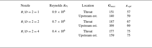
, corresponding to a Reynolds number in the transitional regimes experimentally observed for each nozzle. Table 2 summarises the results found.
Difference between the transient growth calculation performed at nozzle throat and upstream of nozzle throat.

Gain
 $G_{\textit{max}}$
maps of the nozzle boundary layer computed with
 $\varGamma = 10^{-3}$
and
 $M = 1$
: (a)
 ${\textit{Re}}_{\delta _1} = 1000$
; (b)
 ${\textit{Re}}_{\delta _1} = 2000$
; (c)
 ${\textit{Re}}_{\delta _1} = 3000$
; (d)
 ${\textit{Re}}_{\delta _1} = 5000$
.

The difference between the estimation at the nozzle throat and upstream of the nozzle throat is rather small: the gain is lower by a few per cent, and the optimal distance associated with the gain is practically the same. This is due to the boundary layer being small compared the nozzle radius and the increase in boundary layer thickness negligible. Hence the distance required to reach maximum gain is small compared with the nozzle size. In the case
 $R/D = 2$
at
 ${\textit{Re}}_t = 0.7\times 10^6$
, the optimal distance
 $x_{\textit{opt}} = 69$
corresponds to approximately
 $4\,\%$
of the inlet radius. In this condition, performing the computation at the nozzle throat is thus a good approximation. The short development of unsteady streaks also strengthen the relevance of the locally parallel approach, as non-parallel flow effects can be neglected.
6.2. Free stream perturbation transition model
To compare the experimental results with the theoretical ones, gain maps as a function of
 $\omega$
and
 $\beta$
are computed for each nozzle at Reynolds numbers ranging from
 ${\textit{Re}}_t = 0.1\times 10^6$
to
 ${\textit{Re}}_t = 2\times 10^6$
. For each nozzle and each Reynolds number, the maximum gain
 \begin{equation} {G}_{{\textit{max}}}(R/D, {\textit{Re}}_t) = \max _{x,\omega ,\beta } \textit{G}(\omega , \beta ,x,R/D,{\textit{Re}}_t), \end{equation}
is used for the comparison with the experiments. Following the observations of the previous section, the stability computations are performed at the nozzle geometrical throat.
The amplitude growth N-factor,
 $N = \ln ( \sqrt { G_{\textit{max}}} )$
, is used to estimate the transition
 ${\textit{Re}}$
number. The evolution of the N-factor as a function of
 $R_e$
for each nozzle geometry is shown in figure 26. As expected,
 $N$
increases with the Reynolds number for each nozzle. One should bear in mind that
 $G_{\textit{max}}$
is not typically achievable under practical conditions, since it requires optimal perturbations at the inlet to be realised. Nevertheless, it represents a worst-case scenario for transition that can serve to tune a simple model in the present case.
The N-factor as function of Reynolds number
 ${\textit{Re}}_t$
from the transient growth formulation.

At a given Reynolds number
 ${\textit{Re}}_t$
, the value of N decreases as the ratio
 $R/D$
decreases. This is due to the higher flow acceleration obtained through the smaller throat radius, resulting in a thinner boundary layer at the nozzle throat, a smaller boundary-layer based Reynolds number and therefore a lower gain.
The thinning of the boundary layer with increasing
 ${\textit{Re}}_t$
also reduces the relative curvature
 $\varGamma = \delta ^*/R$
, reducing its lift-up effect on low frequency streaks. As seen before, the frequency on which the maximum gain is found increases monotonically with
 $\varGamma$
. In the limit
 $\varGamma \rightarrow 0$
, we find a maximum gain at
 $\omega = 0$
. On the contrary, when the Reynolds number is low, with a thicker boundary layer, the curvature effects are important and result in an increase in the frequency of the optimal unsteady streaks. Each nozzle thus has a different optimal perturbation frequency, depending on the relative curvature, which evolves with the Reynolds number.
The N-factor curves alone do not allow the determination of the transition Reynolds number. In order to obtain the transition Reynolds number, empirical relationships determined by experience must be used. For flat-plate boundary layers, where the TS wave is unstable, the N-factor at which transition happens is usually around 9 for low turbulence intensity wind tunnel. This value is subject to variation depending on the turbulence intensity of the incoming flow (see van Ingen Reference van Ingen2008). In the present case, the N-factor cannot be directly compared with flat plate boundary layers, as the transition mechanism is not related to the modal growth of the unstable TS wave. Furthermore, due to experimental constraints, the nozzle considered is confined on one side by a flat wall, in lieu of a symmetric convergent section. An impact on the transition Reynolds number cannot be excluded. The observed trends are, however, well reproduced by the theoretical model, which suggests that curvature and acceleration on the nozzle side have a larger impact on transition than the flat-wall wall boundary layer.
In order to evaluate the transition N-factor of our current nozzle flow, we propose to use the experimental observations. The nozzle data obtained at
 $R/D = 4$
and
 ${\textit{CR}}=5$
are used to calibrate the model by selecting the Reynolds number
 ${\textit{Re}}_t^i$
associated with the incipient transition and
 ${\textit{Re}}_t^f$
associated with the fully transitioned boundary layer, resulting in an initial and final
 $N$
-factors given by
 \begin{equation} {\textit{Re}}_t^i = 0.25 \times 10^6 \rightarrow N^i = 2.4 \,\,\,\,\text{and} \,\,\,\, {\textit{Re}}_t^f = 0.61 \times 10^6 \rightarrow N^f = 2.75. \end{equation}
Assuming that
 $N^i$
and
 $N^f$
are independent of the tested nozzle geometry for the same contraction ratio, the latter
 $N$
-factor values are used to estimate the transition Reynolds numbers for the two other nozzles geometries:
 $R/D = 2$
and
 $R/D = 1$
. The results are shown in figure 27 and compared with the experimental measurements.
Reynolds number of transition for the tested nozzles. Comparison between experimental observation (
 ${\textit{CR}}=5$
) and transition model. The transition begins on the left-hand marker, the transition ends on the right-hand marker. The line represents the transitional regime.

The model describes a behaviour similar to that of the experiments: a decreasing radius of curvature increases the Reynolds number at which the transition occurs, which is associated with the reduction in the size of the boundary layer when the radius of curvature is smaller. The model also predicts the widening of the transitional zone as
 $R/D$
decreases.
For the case
 $R/D = 1$
, the width of the transition zone is correctly captured, but there is a mismatch between the model and the experimental results on the Reynolds number at which the transition first occurs. This discrepancy is most likely due to the limitations of the boundary layer model used as a base flow for the transient growth calculation. Indeed, the boundary layer model uses a quasi-one-dimensional approach for the calculation of the pressure gradient and the Mach number at the throat is set at
 $M=1$
. However, it has been shown and calculated by Hall (Reference Hall1962) that small
 $R/D$
ratios in nozzles cause important 2-D effects, such as a non-negligible centrifugal force which modifies the pressure gradient along the wall and the emergence of a supersonic pocket near the wall at the nozzle throat. For small
 $R/D$
ratios, a boundary layer model taking into account these effects should be used. Moreover, the reader must also note that the effect of free stream turbulence intensity is not taken into account in the calibration procedure. For example, for the
 $R/D = 4$
nozzle, the turbulence intensities are
 \begin{align} {\textit{Re}}_t^i = 0.25 \times 10^6 \rightarrow {\textit{Tu}}^i = 0.38 \,\% \,\,\, \text{and} \,\,\, {\textit{Re}}_t^f = 0.61 \times 10^6 \rightarrow {\textit{Tu}}^i = 0.48 \,\%, \end{align}
while the
 $R/D = 1$
nozzle has transition points and turbulence intensity corresponding to
 \begin{align} {\textit{Re}}_t^i = 0.46 \times 10^6 \rightarrow {\textit{Tu}}^i = 0.48 \,\% \,\,\,\text{and} \,\,\, {\textit{Re}}_t^f = 1.42 \times 10^6 \rightarrow {\textit{Tu}}^i = 0.57 \,\%. \end{align}
A higher turbulence intensity is likely to cause an earlier transition, which may also partly explain the discrepancy observed between the model and the measurement.
7. Discussion on the disturbances’ origins
The spatial transient growth analysis is based on the optimal disturbance theory, where we have selected the optimal perturbation in order to maximise energy growth. In experimental configurations, there are two main candidates to introduce disturbances into the boundary layer: the first is free stream forcing due to external disturbances, such as free stream turbulence level or acoustic waves; the second is wall roughness, where distributed or isolated roughness elements can introduce disturbances in their wake.
7.1. Disturbances from distributed roughness elements
The presence of distributed roughness is one of the possible factors leading to the transition. In order to evaluate the possible impact of the wall roughness onto the optimal perturbations, the measured wall roughness size of our nozzles is compared with the velocity field of the steady optimal perturbation, i.e. at
 $\omega = 0$
, in figure 28. To aid the comparison, an idealised sinusoidal roughness, at the optimal perturbation wavelength, of the same arithmetic roughness
 ${\textit{Ra}}$
is plotted with the real-measured surface.
Steady optimal disturbance flow field
 $\omega = 0$
,
 $\beta =0.95$
at
 ${\textit{Re}}_t = 10^6$
,
 $R/D = 2$
and
 ${\textit{CR}} =5$
. The dashed grey line represents the boundary layer edge. Near
 $y=0$
, the plain straight line is the ideal flat wall. The plain curve is the measured rough wall
 ${\textit{Ra}}/D = 65.6 \times 10^{-6}$
. The dashed line is an ideal sinusoidal wall that has the same
 ${\textit{Ra}}/D$
as the measured wall and a wavenumber corresponding to the optimal disturbance
 $\beta = 0.95$
.

Although the roughness used here for comparison is the largest
 ${\textit{Ra}}$
that we tested, it can be noticed qualitatively that the heights of the ideal and measured roughness are an order of magnitude smaller than the optimal stationary disturbance leading to streaks and transition. The lowest surface roughness of our nozzle in this study is two orders of magnitude smaller than the optimal perturbation.
Power spectral density of the surface roughness. The shaded area corresponds to the optimal gain
 $G_{\textit{max}}$
obtained from the transient growth formulation at the corresponding wavenumber
 $\beta$
for steady disturbances
 $\omega = 0$
for the nozzle
 $R/D=2$
at
 ${\textit{Re}}_t = 10^6$
. Darker correspond to higher gains.

The figure 29 shows the power spectral density
 $S_{xx}$
of the wall roughness profile for each roughness level, scaled by the displacement thickness of the boundary layer
 $\delta ^*$
at
 ${\textit{Re}}_t = 10^6$
. As expected, we notice that the roughness over spectral density amplitudes increase with the overall roughness level. For each roughness, the power distribution in the spectrum is as follows: it starts with a flat distribution in the lowest wavenumber range, as white noise would produce, and, at a threshold wavenumber, consistently decreases. The threshold wavenumber at which the cascade starts depends on the surface roughness: the lower the roughness, the higher the threshold. The grey shaded area indicates that high streaks gain is likely to occur in the range
 $\beta \approx [0.5 {-} 2]$
. We can see that the wall surface actually contains roughness of similar wavelength that could initiate the perturbation in the flow. However, the reader must notice that the amplitude of the associated roughnesses is 3–5 orders of magnitude smaller than the boundary layer displacement thickness, and therefore smaller than the actual extent of the optimal perturbation into the boundary layer. Hence, in the experiments carried out, the roughness did not reach the level necessary to affect the transition Reynolds numbers.
7.2. Disturbances from isolated roughness elements
Isolated-roughness elements are known to cause transition to turbulence provided they are sufficiently large compared with the thickness of the boundary layer. In a numerical investigation, Bernardini et al. (Reference Bernardini, Pirozzoli, Orlandi and Lele2014) performed a parametric study of boundary layer transition induced by an isolated roughness element. They varied the shape, the height, the Reynolds number and the Mach number and found that a Reynolds number
 ${\textit{Re}}_{2k}$
based on the height of the roughness elements
 $k$
, the velocity
 $u_k$
and density
 $\rho _k$
evaluated in the undisturbed boundary layer at the height
 $k$
and the viscosity evaluated at the wall
 $\mu _k$
,
 \begin{equation} {\textit{Re}}_{2k} = \dfrac {\rho _k u_k k}{\mu _k}, \end{equation}
is convenient to describe the critical roughness height that will cause the transition to turbulence. Depending on the roughness shape, the wake introduced behind the obstacle would breakdown to turbulence if
 ${\textit{Re}}_{2k} \gt [400 {-} 700]$
. Using the analytical formulation of the boundary layer we consider, it is possible to calculate this Reynolds number as a function of the roughness height, and thus to determine the critical roughness height, that would lead to transition, as a function of
 ${\textit{Re}}_t$
. Figure 30 presents the evolution of the critical height of a roughness element
 $k/D$
that would cause transition at the nozzle throat as a function of
 ${\textit{Re}}_t$
for the three-nozzle geometry
 $R/D =[1,2,4]$
. As can be seen, the critical roughness height diminishes for increasing
 ${\textit{Re}}_t$
, as a result of boundary layer thinning. One can see that the nozzle inlet radius has a small effect on the critical roughness height.
Evolution of the critical roughness height based on the Reynolds number
 ${\textit{Re}}_{2k}$
as a function of
 ${\textit{Re}}_t$
. The dashed and full lines correspond to
 ${\textit{Re}}_{2k} = 400$
and
 ${\textit{Re}}_{2k} = 700$
, respectively, for the three nozzle
 $R/D = [1,2,4]$
. Lighter shades correspond to bigger
 $R/D$
.

We now compare this theoretical result with the experimental nozzle investigated. Each nozzle wall profile has been measured at three spanwise locations at the nozzle throat and the highest peak measured for each measurement area is reported in table 3. The maximum observed peaks heights stand between
 $k/D \approx [0.1 {-} 0.3] \times 10^{-3}$
,
 $k/D \approx [0.3 {-} 0.4] \times 10^{-3}$
and
 $k/D \approx [0.4 {-} 1] \times 10^{-3}$
for smooth, medium and rough surface finish, respectively. For the medium and smooth surface finish, the peak value stand below the threshold value for roughness-induced transition, according to figure 30. However, the rough surface finish of the nozzle
 $R/D =2$
is less even and shows peaks up to
 $k/D = 1.04 \times 10^{-3}$
, which become critical in the transitional
 ${\textit{Re}}$
range for that nozzle. Transition spots due to isolated roughness are actually visible on the infrared images presented figure 31: the temperature field presents elongated bright triangular spots, indicating roughness-induced turbulence, which is absent on the infrared image of the medium surface finished nozzle at the same Reynolds number. As one can see, the rough surface finish nozzle presents both a diffuse bright shade, expected from an even transition due to non-modal growth of perturbation, and triangular shaped bright spots superimposed, indicating isolated roughness transition mechanisms competing for the transition. In figure 7, where we have compared the transition occurrence as a function of surface finish, the occurrence of isolated roughness-induced transition was not apparent. The transition started first because of free stream turbulence and non-modal growth, before the boundary layer became small enough (due to the increase in Reynolds number) to show the influence of isolated roughness elements. Slightly higher roughness peaks would have probably caused an even earlier transition.
Isolated roughness peaks measured on each nozzle wall, at throat.

Enhanced infrared images of
 $R/D =2$
nozzle’s wall:
 ${\textit{Re}}_t = 0.79 \times 10^6$
; (a) medium surface finish; (b) rough surface finish. The position
 $x/D = 0$
correspond to the throat location, the thin vertical line near
 $x/D= -1.8$
is where the nozzle starts to converge. Flow is from left to right.

8. Conclusion
The experimental study of the boundary layer transition in planar nozzles allowed to highlight the impact of different parameters on the transition process. The roughness, at the scales studied, did not have a determining role on the transition. The transition from the boundary layer to the nozzle throat is complete before roughness effects can appear. On the contrary, the curvature of the nozzle has an important impact on the transition point: the smaller the radius of curvature, the higher the Reynolds number of transition. The range over which the intermittency between laminar and turbulent boundary layer is observed is larger for small radii of curvature. These observations point towards transition being most likely caused by perturbations present in the free stream and non-modal growth mechanism.
This path to turbulence is typically modelled using the linear stability theory. For the nozzle flow considered in this study, the favourable pressure gradient at the throat stabilises the familiar TS wave and the transition is likely due to a transient growth mechanism forming streaks in the downstream direction at non-zero frequencies. Centrifugal forces, due to curvature of the nozzle, tend to reduce the overall gain of the process and a mechanism explaining how streaks lose their strength has been proposed. The development length of these streaks is short, of the order of
 $4\,\%$
of the nozzle radius, making the transient growth mechanism a credible model for the transition inside the nozzles. The Reynolds number at which the transition occurs is predicted using a dedicated
 $N$
-factor, and shows similar trends with the experimental observations. Non-modal transition occurs at values of
 $N \approx 2.5$
in the present experiment. Although, this value is low compared with classical
 $N = 9$
for modal growth, it nonetheless represents an amplitude growth of an order of magnitude. Further work is, however, necessary to determine if the lower value of
 $N$
is associated with the streak’s unsteadiness or an increase of turbulence intensity in the nozzle.
Another important parameter when considering the transition Reynolds number is the streak breakdown mechanism. The studies of Andersson et al. (Reference Andersson, Brandt, Bottaro and Henningson2001) and Paredes, Choudhari & Li (Reference Paredes, Choudhari and Li2017) about steady streaks shows that there exist secondary modal instabilities that have consequent growth rates. Unsteady streaky base flows were investigated in Vaughan & Zaki (Reference Vaughan and Zaki2011) and it is found that unsteady streaks become unstable at lower amplitudes than steady ones. Further investigation with 2-D streaky baseflow could provide more insights on the transition mechanism in the present case, providing more precise transition N factors.
Finally, the wall roughness was studied in detail and was found too small compared with the size of the optimal perturbation to have an influence on the transition. However, the statistical nature of the wall roughness quantification allows for isolated roughness elements, considerably larger than the average ones, to potentially cause transition in the roughness wake. When the surface finish is coarsened, it has been experimentally observed that there is competition between a free stream disturbance associated transition and isolated-roughness-induced transition. However, for the roughness levels required by industry standards for the manufacture of gas flow metering nozzles, the isolated-roughness transition is unlikely to occur and transition should only be associated with free stream disturbances, for which the transient growth mechanism seems to be a correct representation of the mechanism at play.
Acknowledgements
B.Z. would like to thank I. Padilla from The von Kármán Institute for kindly providing data for code validation.
Funding
We gratefully acknowledge the financial support provided by CESAME-EXADEBIT. We are grateful to the Region Nouvelle-Aquitaine for their financial support through the funding of the transonic transition project. The CPER-FEDER is also thanked for their support via the Transport program.
Declaration of interests
The authors report no conflict of interest.
Appendix A. Transonic spectra
A.1. Transonic eigenvalue spectrum
To the authors’ knowledge, the spectra of transonic boundary layers are scarcely, if at all, studied in the literature. To assess the stability of the boundary layer and to carry out the transient growth study, it is important to understand the origin and role of each eigenmode. Therefore, to facilitate the discussion, we recall in figure 32 the composition of the spectra of subsonic and supersonic boundary layers, where we identify the different branches composing the eigenspectrum as follows:
-
(i)
 ${\textit{BA}}_e$
, evanescent acoustic branches;
-
(ii)
${\textit{BA}}_p$
, propagative acoustic branches; -
(iii)
$A_n$
, evanescent boundary layer acoustic modes; -
(iv)
$BC$
, free stream convected branch modes; -
(v) Discrete modes, discrete modes of the boundary layer.


Boundary layer typical eigenspectra for a subsonic flow (a) and a supersonic one (b).

The superscript indicates the propagation direction of the corresponding modes:
 $^+$
for modes propagating downstream and
 $^-$
for modes propagating upstream.
The supersonic eigenvalue spectrum exhibits two interesting features: the boundary layer modes
 $A_n$
, which are stable, and the displacement of the acoustic branches onto the real axis. It is important to identify these characteristics in order to assess the modal stability of the boundary layer, but also for the formulation of transient growth, which requires the use of a reduced basis composed of eigenvectors propagating in the
 $x^+$
direction.
In order to have a clearer understanding of the spectra of transonic boundary layers, the eigenvalue spectra are presented in figure 33 for a flow with Mach number varying from
 $M=0.95$
to
 $M=1.05$
. Initially, at
 $M=0.95$
, the modes are arranged in the spectrum similarly to the subsonic case. As the Mach number approaches unity, the modes from the subsonic
 ${\textit{BA}}_e^+$
branch gradually transition from vertical to horizontal alignment, aligning with the neutral axis
 $\alpha _i = 0$
to become the
 ${\textit{BA}}_p^+$
branch of the supersonic boundary layer spectrum. The slow acoustic branches
 ${\textit{BA}}_p^-$
and
 ${\textit{BA}}_e^-$
from the subsonic spectrum progressively degenerate towards negative
 $\alpha _i$
values. The displacement of the evanescent acoustic branches
 ${\textit{BA}}_e^+$
and
 ${\textit{BA}}_e^-$
reveals the boundary layer modes
 $A_n^+$
and
 $A_n^-$
. These modes visibly originate from the acoustic branches, reinforcing the idea that they are acoustic modes evolving within the boundary layer.
With increasing Mach number, the slow acoustic branch
 ${\textit{BA}}_p^-$
of the supersonic spectrum appears with positive values of both
 $\alpha _i$
and
 $\alpha _r$
. In the supersonic regime, this branch approaches the neutral axis and becomes predominantly propagative (
 $\alpha _i = 0$
) at
 $M=1.05$
. At
 $M=1$
, multiple acoustic branches coexist in the spectrum: the supersonic branches
 ${\textit{BA}}_p^-$
(denoted by
 $\unicode{x2461}$
in the
 $M=1$
spectrum) and
 ${\textit{BA}}_p^+$
(denoted by
 $\unicode{x2460}$
), as well as the subsonic acoustic branches
 ${\textit{BA}}_p^-$
and
 ${\textit{BA}}_e^-$
(denoted by
 $\unicode{x2462}$
). The positioning of the two slow acoustic branches (
 $\unicode{x2461}$
and
 $\unicode{x2462}$
) is exceptional, as their imaginary parts are non-zero. This phenomenon occurs only for transonic flow conditions. At
 $M=1$
, no propagative modes exist for these two acoustic branches; all of their modes are evanescent.
Blasius boundary layer eigenspectrum for Mach numbers in between
 $M=0.95$
and
 $M=1.05$
, and for
 $\beta =0$
,
 $\omega = 0.15$
,
 ${\textit{Re}} = 1000$
.

The free stream convected modes are, for their part, only marginally affected by the transonic transition. Their position in the spectrum is only slightly modified as the flow transitions from subsonic to supersonic.