1 Introduction
A displacement flow occurs when one fluid pushes another one, usually within a confined geometry. Displacement flows are studied from various perspectives as they appear in a variety of natural phenomena and industrial applications. Examples of relevant industrial applications may include oil/gas well construction or production (pipelining) in the petroleum industry (see e.g. Nelson & Guillot Reference Nelson and Guillot2006) and coating and co-extrusion flows in manufacturing (see e.g. Schweizer & Kistler Reference Schweizer and Kistler2012), to name a few. Miscible flows are widespread and density and viscosity ratios between the phases are quite common. These flows frequently occur in pipes, but also in annuli, rectangular ducts and other flow geometries. Although miscible displacement flows in pipes and two-dimensional (2-D) channels have been recently studied in depth (e.g. Taghavi et al. Reference Taghavi, Alba, Seon, Wielage-Burchard, Martinez and Frigaard2012b and Alba, Taghavi & Frigaard Reference Alba, Taghavi and Frigaard2013a ), our knowledge of the effects of the flow geometry on these flows is limited, perhaps since these are fairly complex flows and a large number of parameters are involved. In this study, which combines theory and experiments, our goal is to provide basic understanding of displacement flows occurring in rectangular ducts.
In the current work, we consider buoyant displacement flows in a rectangular channel oriented at near-horizontal inclinations. The two fluids are miscible. We consider a case where the ratio of the length to the hydraulic diameter of the channel is large. The configuration of our interest is density unstable, where one fluid displaces a slightly lighter fluid downwards. In near-horizontal inclinations, strong transverse buoyancy forces help to segregate the phases, leading to stratified fluid layers. Thus, we may expect the displacement flow to be structured/laminar for certain ranges of the relevant dimensionless flow parameters. We also concentrate on the condition where the density difference is small so that the Boussinesq approximation becomes applicable. Moreover, in addition to the density ratio and the channel cross-section aspect ratio, in general we consider that a viscosity ratio between the two fluids may be also present, as a third flow parameter. Finally, although we are dealing with miscible fluids, we assume the corresponding Péclet number of the displacement flow to be sufficiently large, the significance of which is that, within the time scales of our interest, the fluids do not mix unless due to hydrodynamic effects. In other words, we are away from dispersive flow regimes.
In the absence of buoyancy, miscible displacement flows at high Péclet numbers have been studied extensively; see e.g. Chen & Meiburg (Reference Chen and Meiburg1996), Petitjeans & Maxworthy (Reference Petitjeans and Maxworthy1996), Rakotomalala, Salin & Watzky (Reference Rakotomalala, Salin and Watzky1997), Yang & Yortsos (Reference Yang and Yortsos1997). These analytical, computational and experimental studies demonstrate that sharp interfaces between the fluids may be found for a wide range of flow parameters. Therefore, these flows approach their immiscible limit at zero surface tension. When a density difference is present, miscible displacement flows at high Péclet numbers have been studied in vertical ducts; see e.g. Joseph & Renardy (Reference Joseph and Renardy1993), Lajeunesse et al. (Reference Lajeunesse, Martin, Rakotomalala and Salin1997, Reference Lajeunesse, Martin, Rakotomalala, Salin and Yortsos1999), Sahu et al. (Reference Sahu, Ding, Valluri and Matar2009b ).
At zero imposed displacement flow velocities, our buoyant flows are equivalent to exchange flows, for which the literature is extensive and fairly well developed. For example, the case of exchange flows in inclined pipes was studied experimentally in depth by Seon et al. (Reference Seon, Hulin, Salin, Perrin and Hinch2004, Reference Seon, Hulin, Salin, Perrin and Hinch2005, Reference Seon, Hulin, Salin, Perrin and Hinch2006, Reference Seon, Znaien, Salin, Hulin, Hinch and Perrin2007a ,Reference Seon, Znaien, Salin, Hulin, Hinch and Perrin b ). Their work concentrated on iso-viscous fluid flows at small density differences. However, buoyancy forces were still relatively strong and therefore the inclination angle was an important factor in characterizing various flow regimes. They found that the flow was in a viscous state in near-horizontal angles while it transitioned to an inertial state at higher inclinations. Hallez & Magnaudet (Reference Hallez and Magnaudet2008) performed numerical simulations and confirmed the qualitative picture of Seon et al. (Reference Seon, Hulin, Salin, Perrin and Hinch2005, Reference Seon, Hulin, Salin, Perrin and Hinch2006), although their focus was primarily on inertial flows. They pointed out striking differences between the flows in 2-D channels and those in 3-D pipes and square channels. For example, they discovered that coherence and persistence of vortices in two dimensions result in a periodic cut of the pure fluid channels that feed the front. It is also relevant to mention a number of exchange flow studies with significant buoyancy and inertia, concerning vertical pipe flows, e.g. Debacq et al. (Reference Debacq, Hulin, Salin, Perrin and Hinch2003), low Reynolds number flows, e.g. Huppert & Hallworth (Reference Huppert and Hallworth2007) and Beckett et al. (Reference Beckett, Mader, Phillips, Rust and Witham2011), as well as buoyancy-driven miscible fluid flows over near-horizontal surfaces in geophysical contexts, e.g. Benjamin (Reference Benjamin1968), Shin, Dalziel & Linden (Reference Shin, Dalziel and Linden2004) and Birman et al. (Reference Birman, Battandier, Meiburg and Linden2007).
Buoyant miscible displacement flows in pipes and 2-D channels have been recently studied in depth, both for near horizontal (e.g. Taghavi et al.
Reference Taghavi, Seon, Martinez and Frigaard2010, Reference Taghavi, Seon, Wielage-Burchard, Martinez and Frigaard2011, Reference Taghavi, Alba, Seon, Wielage-Burchard, Martinez and Frigaard2012b
) and away from horizontal inclinations (see, e.g. Alba et al.
Reference Alba, Taghavi and Frigaard2013a
). For progressively increasing imposed flow velocities added to a pipe exchange flow, Taghavi et al. (Reference Taghavi, Seon, Martinez and Frigaard2010) classified three displacement flow regimes based on global displacement flow behaviours, i.e. an exchange flow dominated regime, an imposed flow dominated regime and a fully mixed regime. They found that the first regime is associated with counter-current streams of light and heavy fluids whereas the second regime is linked to a stabilization effect due to the presence of an imposed flow. The last regime is about turbulent mixing between the displacing and displaced fluids when the imposed flow is itself turbulent. An interesting and counterintuitive aspect in their findings is that the stabilization effect of the imposed flow is observed even when the corresponding exchange flow is highly inertial. Taghavi et al. (Reference Taghavi, Seon, Wielage-Burchard, Martinez and Frigaard2011) found that the transition between the exchange and imposed flow dominated regimes occurs at a marginal state where the light displaced fluid remains in a stationary layer form, on the upper side of the pipe. Although the fluid within the displaced layer is in counter-current motion, its net flux is zero and consequently the layer is stationary for long experimental times, e.g.
 ${\sim}O(10^{3})\times \bar{t}$
, where
 $\bar{t}$
is the characteristic flow time. Experiments and simulations of Taghavi et al. (Reference Taghavi, Seon, Wielage-Burchard, Martinez and Frigaard2011, Reference Taghavi, Alba, Seon, Wielage-Burchard, Martinez and Frigaard2012b
) showed that there are similarities and differences between pipe and 2-D channel displacement flows. In terms of similarities, they found that the overall experimental regime classification is valid in 2-D simulations. This, in particular, includes the marginal stationary layer state. In terms of differences, the laminarization effect of the imposed flow is not significant for 2-D channel flows. Another difference is that the imposed flow dominated regime in two dimensions is not slump-type (i.e. two-layer); instead, the displacing fluid advances more or less in the middle of the 2-D channel so that a three-layer flow model is accordingly more appropriate. Taghavi et al. (Reference Taghavi, Seon, Wielage-Burchard, Martinez and Frigaard2011, Reference Taghavi, Alba, Seon, Wielage-Burchard, Martinez and Frigaard2012b
) also presented a comprehensive classification of displacement flows, based on studying the behaviours of the displacement trailing front, when the mean imposed flow velocity is gradually increased from zero. They found that for certain flow parameters, it is possible for there to exist a sustained-backflow regime, where buoyancy is sufficiently strong to maintain an upward motion of the trailing front. For larger imposed flows, there exists a marginal stationary interface flow state, where the trailing front initially advances upward but stops for the duration of the experiment. For even larger imposed flows, they discovered that a temporary backflow occurs when the trailing front moves upstream only for a finite time, but it eventually reverses and becomes displaced downstream. Finally, at very large imposed flows, they observed an instantaneous displacement, for which the trailing front moves directly downstream.
Concerning the flow geometry of the current wok, i.e. a rectangular channel, there exist only a few relevant studies in the literature. For example, Martin et al. (Reference Martin, Rakotomalala, Talon and Salin2011) have studied, both theoretically and experimentally, iso-viscous exchange flows in a horizontal channel with a rectangular cross-section, for a wide range of aspect ratios. Their work has provided validated predictions to the time evolution of the interface between the two interpenetrating fluids, in the regime where buoyancy (as a driving force) is balanced by viscosity (as a dissipative force). Through a lattice Boltzmann approach, Redapangu, Sahu & Vanka (Reference Redapangu, Sahu and Vanka2013) have studied buoyant displacement flows of two immiscible fluids in a square duct. They have explored a range of density and viscosity ratios for different values of the duct inclination angle, concluding that the flow dynamics in square and 2-D channels are completely different. For example, they have reported that the displacement is relatively more coherent in a square channel than in a 2-D channel. It is also relevant to mention the experimental study of Malham et al. (Reference Malham, Jarrige, Martin, Rakotomalala, Talon and Salin2010) on the lock-exchange flow with an autocatalytic reaction front, which concerns the front propagation in horizontal rectangular channels, for a wide range of aspect ratios. Finally, Matson & Hogg (Reference Matson and Hogg2012) have studied gravitationally driven exchange flows of viscous fluids with different densities in horizontal channels, using theoretical and experimental approaches. For certain cases of exchange flows in a rectangular cross-section channel, they have found similarity forms for the shape of the evolving interface between the two fluids.
There exist two obvious limiting cases for rectangular channel displacements: (i) flow in a channel of very small aspect ratio (porous media or vertical Hele-Shaw cell); (ii) flow in a channel of very large aspect ratio (horizontal Hele-Shaw cell). In an appealing study, Martin et al. (Reference Martin, Rakotomalala, Talon and Salin2011) have derived and collected several spreading diffusion coefficients for the exchange flow configuration in these limiting cases. For displacement flows, Zheng et al. (Reference Zheng, Guo, Christov, Celia and Stone2015a ) have recently extended the work of Bear (Reference Bear1972) and Huppert & Woods (Reference Huppert and Woods1995) to consider the flow in the porous media limiting case, in the presence of density and viscosity ratios. They have shown that in the early time period the fluid motion is mainly driven by buoyancy, while in the late time period it is determined by the imposed displacement flow velocity. The other limiting case, i.e. a two-dimensional viscous flow between two parallel horizontal boundaries, has been investigated by Taghavi et al. (Reference Taghavi, Seon, Martinez and Frigaard2009) and Zheng, Rongy & Stone (Reference Zheng, Rongy and Stone2015b ). In this body of work, the reduced model equations are relatively simple; therefore, it is possible to find simple expressions (e.g. analytical, similarity and asymptotic forms) for the flux functions and the interface evolution.
Some of the contributions of the current work are as follows. First, we develop for the first time a semi-analytical model for displacement flows in rectangular channels of arbitrary cross-section aspect ratios, in the presence of viscosity and density contrasts. Second, we perform a large number of displacement flow experiments to draw meaningful comparisons with the model. Third, based on the model and experimental results, we present a complete classification of various displacement regimes and provide leading-order predictions to flow behaviours in each regime. Our work can be regarded as a step forward to better understand rectangular channel displacements, which are studied much less compared to their pipe counterparts, and eventually aid in quantifying the flow geometry effects on buoyant displacement flows.
The paper is structured as follows. In § 2, we present the problem of our study as well as the flow governing equations. In § 3, we develop a semi-analytical model for Newtonian displacements flows in rectangular ducts. In § 4, we discuss the model results concerning various interfacial behaviours. In § 5, we present our iso-viscous displacement flow experiments performed in a long duct with a nearly square cross-section. The paper ends in § 6 with a summary and conclusions.
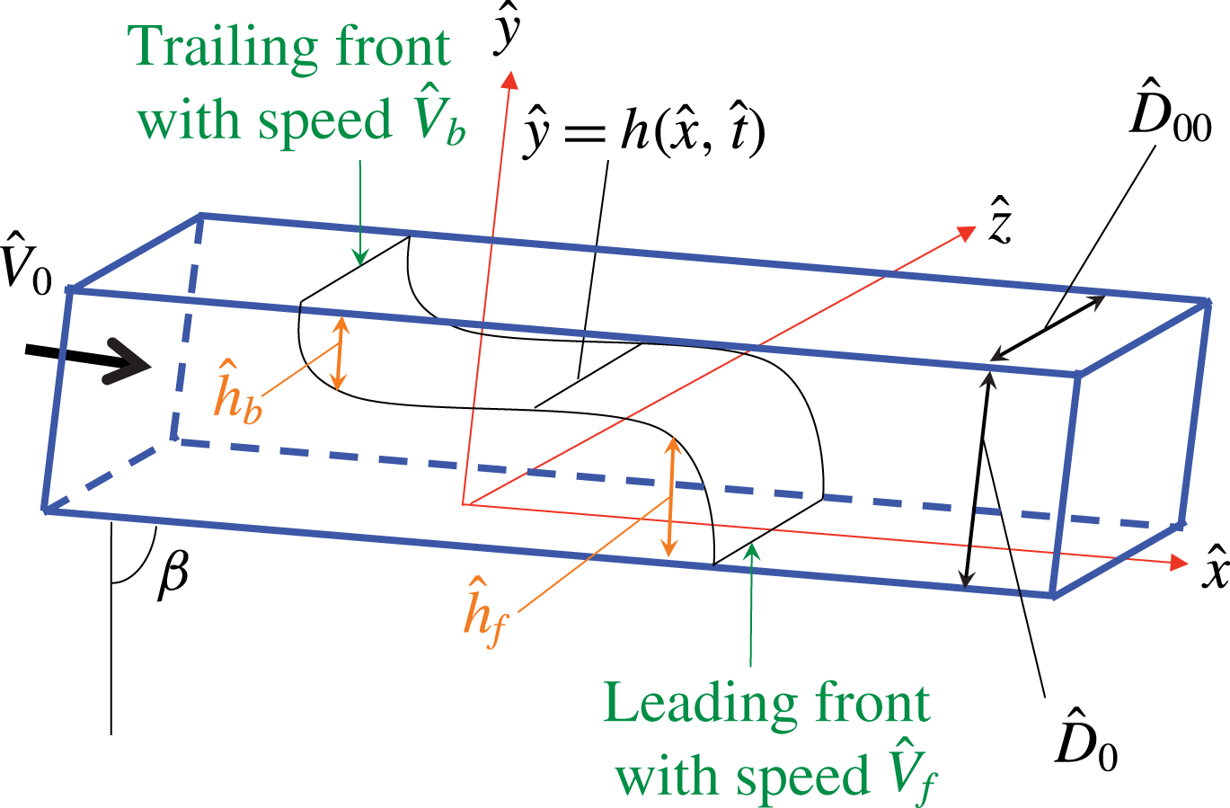
Schematic of the displacement flow geometry considered.

2 Problem setting and governing equations
We consider a displacement flow in a long rectangular duct, for which the cross-section has height
 $\hat{D}_{0}$
and depth
 $\hat{D}_{00}$
, as illustrated in figure 1. The lower wall of the rectangular duct is oriented at an angle
 $\unicode[STIX]{x1D6FD}\approx \unicode[STIX]{x03C0}/2$
with respect to the duct vertical position. The lower part of the duct is filled with a lighter fluid (fluid
 $L$
), which is later displaced by a heavier fluid (fluid
 $H$
). As time grows, we take into account only mechanically stable displacement flows: fluid
 $H$
propagates at the bottom of the duct and fluid
 $L$
at the top so that fluid
 $H$
lies beneath fluid
 $L$
. The heavy displacing fluid is injected into the duct at a distance far away from the initial sharp interface (localized to
 $\hat{x}=0$
). The mean injection imposed velocity is
 $\hat{V}_{0}$
. Figure 1 depicts the Cartesian coordinates
 $(\hat{x},{\hat{y}},\hat{z})$
and the geometrical parameters of the flow. We assume that the fluids are both Newtonian but they may have different dynamic viscosities, i.e.
 $\hat{\unicode[STIX]{x1D707}}_{H}$
and
 $\hat{\unicode[STIX]{x1D707}}_{L}$
for the heavy and light fluids, respectively. Although the fluids of our interest are miscible, we consider the large Péclet number limit (
 $Pe\equiv \hat{V}_{0}\hat{D}_{0}/\hat{D}_{m}$
with
 $\hat{D}_{m}$
being the molecular diffusion coefficient), which implies that no significant mixing occurs between the two fluids over the time scales of interest. Therefore, from a modelling perspective, the boundary between two fluids can be seen as a pseudo-interface between two miscible phases where molecular diffusion is neglected. Equally, the boundary can be considered as the interface between two immiscible phases where interfacial tension is neglected; see also Martin et al. (Reference Martin, Rakotomalala, Talon and Salin2011). To render the Navier–Stokes equations dimensionless, we use
 $\hat{D}_{0}$
as length scale and
 $\hat{V}_{0}$
as velocity scale. In addition, we scale time with
 $\hat{D}_{0}/\hat{V}_{0}$
and pressure and stresses with
 $\hat{\unicode[STIX]{x1D707}}_{H}\hat{V}_{0}/\hat{D}_{0}$
. These allow to write the governing equations as
 $$\begin{eqnarray}\displaystyle & \displaystyle [1\pm At]Re[\boldsymbol{u}_{t}+\boldsymbol{u}\boldsymbol{\cdot }\unicode[STIX]{x1D735}\boldsymbol{u}]=-\unicode[STIX]{x1D735}p+\unicode[STIX]{x1D735}\boldsymbol{\cdot }\unicode[STIX]{x1D749}\pm {\displaystyle \frac{Re}{Fr^{2}}}\boldsymbol{e}_{g}, & \displaystyle\end{eqnarray}$$
 $$\begin{eqnarray}\displaystyle & \displaystyle \unicode[STIX]{x1D735}\boldsymbol{\cdot }\boldsymbol{u}=0. & \displaystyle\end{eqnarray}$$
In the equations above,
 $\boldsymbol{u}=(u,v,w)$
represents the velocity,
 $p$
the pressure and
 $\unicode[STIX]{x1D70F}$
the deviatoric stress. In addition,
 $\boldsymbol{e}_{g}=(\cos \unicode[STIX]{x1D6FD},-\text{sin}\,\unicode[STIX]{x1D6FD},0)$
is in directions
 $(x,y,z)$
and the
 $\pm$
refers to the heavy and light fluid layers, respectively. Note that before scaling we have subtracted the mean static pressure gradient from the pressure. In general, there are six dimensionless parameters that govern the problem, four of which appear in (2.1). These four parameters are the inclination angle
 $\unicode[STIX]{x1D6FD}$
, the Atwood number defined as
 $At=(\hat{\unicode[STIX]{x1D70C}}_{H}-\hat{\unicode[STIX]{x1D70C}}_{L})/(\hat{\unicode[STIX]{x1D70C}}_{H}+\hat{\unicode[STIX]{x1D70C}}_{L})$
, the Reynolds number,
 $Re$
, and the densimetric Froude number,
 $Fr$
. The two latter dimensionless numbers are defined as
 $$\begin{eqnarray}Re\equiv {\displaystyle \frac{\hat{V}_{0}\hat{D}_{0}}{\hat{\unicode[STIX]{x1D708}}}},\quad Fr\equiv {\displaystyle \frac{\hat{V}_{0}}{\sqrt{At{\hat{g}}\hat{D}_{0}}}},\end{eqnarray}$$
where
 $\hat{\unicode[STIX]{x1D708}}=\hat{\unicode[STIX]{x1D707}}_{H}/\hat{\unicode[STIX]{x1D70C}}$
is the heavy fluid kinematic viscosity, with
 $\hat{\unicode[STIX]{x1D70C}}$
being the mean density
 $\hat{\unicode[STIX]{x1D70C}}=(\hat{\unicode[STIX]{x1D70C}}_{H}+\hat{\unicode[STIX]{x1D70C}}_{L})/2$
. The two other dimensionless parameters, which do not explicitly appear in (2.1), are the viscosity ratio and the cross-section aspect ratio defined respectively as
 $$\begin{eqnarray}m\equiv {\displaystyle \frac{\hat{\unicode[STIX]{x1D707}}_{L}}{\hat{\unicode[STIX]{x1D707}}_{H}}},\quad \unicode[STIX]{x1D6EC}\equiv {\displaystyle \frac{\hat{D}_{00}}{\hat{D}_{0}}}.\end{eqnarray}$$
Let us limit our attention to flows with relatively small density differences, leading to the consideration of small
 $At$
; thus, the Atwood number itself is not a dimensionless parameter to govern the flow. Instead, a combination of
 $\unicode[STIX]{x1D6FD}$
,
 $Re$
and
 $Fr$
, to represent the balance of axial buoyancy and viscous stresses, becomes relevant:
 $$\begin{eqnarray}\unicode[STIX]{x1D712}={\displaystyle \frac{2Re\cos \unicode[STIX]{x1D6FD}}{Fr^{2}}}.\end{eqnarray}$$
As a result of our scaling, in each cross-section of the duct (assumed to be sufficiently long in direction
 $x$
), we can have
 $$\begin{eqnarray}\int _{0}^{1}\int _{-\unicode[STIX]{x1D6EC}/2}^{+\unicode[STIX]{x1D6EC}/2}u~\text{d}z\,\text{d}y=\unicode[STIX]{x1D6EC}.\end{eqnarray}$$
We assume that a single-valued interface, denoted by
 $y=h(x,t)$
, separates the two pure fluids. In general, we may expect displacement fronts to appear in our flows. As figure 1 shows, we define a leading front with velocity
 $\hat{V}_{f}$
and height
 ${\hat{h}}_{f}$
, and a trailing front with velocity
 $\hat{V}_{b}$
and height
 ${\hat{h}}_{b}$
. The leading and trailing front heights are measured from the bottom and top walls, respectively.
3 Lubrication model
In this section we develop a lubrication model, valid for ‘arbitrary’ values of the buoyancy number (
 $\unicode[STIX]{x1D712}$
), the cross-section aspect ratio (
 $\unicode[STIX]{x1D6EC}$
) and the viscosity ratio (
 $m$
). We assume that the interface between the two fluids is fairly elongated and that inertial effects are not dominant. Note that the latter does not necessarily mean that
 $Re$
is small. In fact, for typical conditions at moderate
 $Re$
, it is possible for the model to be relevant/valid in near-horizontal duct inclinations, in line with the previous studies finding nearly viscous regimes at these angles; see, e.g. Taghavi et al. (Reference Taghavi, Seon, Martinez and Frigaard2010, Reference Taghavi, Seon, Wielage-Burchard, Martinez and Frigaard2011), Taghavi, Alba & Frigaard (Reference Taghavi, Alba and Frigaard2012a
), Taghavi et al. (Reference Taghavi, Alba, Seon, Wielage-Burchard, Martinez and Frigaard2012b
).
To develop our model, we assume that velocities and stresses are continuous across the interface. The interface needs to satisfy a kinematic condition as it is simply advected with the flow. The next step is scaling our equations, using a dimensionless length scale,
 $\unicode[STIX]{x1D6FF}^{-1}\gg 1$
, over which the interface elongates. We assume that
 $\unicode[STIX]{x1D6FF}$
has size
 $\hat{D}_{0}/\hat{L}$
, in which
 $\hat{L}$
denotes the characteristic spreading length of the interface. Defining
 $\unicode[STIX]{x1D6FF}x=X$
,
 $\unicode[STIX]{x1D6FF}t=T$
,
 $\unicode[STIX]{x1D6FF}p=P$
,
 $v=\unicode[STIX]{x1D6FF}V$
, and
 $w=\unicode[STIX]{x1D6FF}W$
and following standard methods (e.g. see Leal Reference Leal2007), we can now rescale our equations to arrive at
 $$\begin{eqnarray}\displaystyle & \hspace{-6.0pt}\unicode[STIX]{x1D6FF}[1\pm At]Re\left[{\displaystyle \frac{\unicode[STIX]{x2202}u}{\unicode[STIX]{x2202}T}}+u{\displaystyle \frac{\unicode[STIX]{x2202}u}{\unicode[STIX]{x2202}X}}+V{\displaystyle \frac{\unicode[STIX]{x2202}u}{\unicode[STIX]{x2202}y}}+W{\displaystyle \frac{\unicode[STIX]{x2202}u}{\unicode[STIX]{x2202}z}}\right]=-{\displaystyle \frac{\unicode[STIX]{x2202}P}{\unicode[STIX]{x2202}X}}+{\displaystyle \frac{\unicode[STIX]{x2202}\unicode[STIX]{x1D70F}_{Xy}}{\unicode[STIX]{x2202}y}}+{\displaystyle \frac{\unicode[STIX]{x2202}\unicode[STIX]{x1D70F}_{Xz}}{\unicode[STIX]{x2202}z}}\pm {\displaystyle \frac{\unicode[STIX]{x1D712}}{2}}+\unicode[STIX]{x1D6FF}^{2}{\displaystyle \frac{\unicode[STIX]{x2202}\unicode[STIX]{x1D70F}_{XX}}{\unicode[STIX]{x2202}X}},\qquad & \displaystyle\end{eqnarray}$$
 $$\begin{eqnarray}\displaystyle & \unicode[STIX]{x1D6FF}^{3}[1\pm At]Re\left[{\displaystyle \frac{\unicode[STIX]{x2202}V}{\unicode[STIX]{x2202}T}}+u{\displaystyle \frac{\unicode[STIX]{x2202}V}{\unicode[STIX]{x2202}X}}+V{\displaystyle \frac{\unicode[STIX]{x2202}V}{\unicode[STIX]{x2202}y}}+W{\displaystyle \frac{\unicode[STIX]{x2202}V}{\unicode[STIX]{x2202}z}}\right] & \displaystyle \nonumber\\ \displaystyle & \qquad \qquad \qquad =-{\displaystyle \frac{\unicode[STIX]{x2202}P}{\unicode[STIX]{x2202}y}}\mp \unicode[STIX]{x1D6FF}{\displaystyle \frac{\unicode[STIX]{x1D712}}{2}}\tan \unicode[STIX]{x1D6FD}+\unicode[STIX]{x1D6FF}^{2}\left({\displaystyle \frac{\unicode[STIX]{x2202}\unicode[STIX]{x1D70F}_{yX}}{\unicode[STIX]{x2202}X}}+{\displaystyle \frac{\unicode[STIX]{x2202}\unicode[STIX]{x1D70F}_{yy}}{\unicode[STIX]{x2202}y}}+{\displaystyle \frac{\unicode[STIX]{x2202}\unicode[STIX]{x1D70F}_{yz}}{\unicode[STIX]{x2202}z}}\right), & \displaystyle\end{eqnarray}$$
 $$\begin{eqnarray}\displaystyle & \unicode[STIX]{x1D6FF}^{3}[1\pm At]Re\left[{\displaystyle \frac{\unicode[STIX]{x2202}W}{\unicode[STIX]{x2202}T}}+u{\displaystyle \frac{\unicode[STIX]{x2202}W}{\unicode[STIX]{x2202}X}}+V{\displaystyle \frac{\unicode[STIX]{x2202}W}{\unicode[STIX]{x2202}y}}+W{\displaystyle \frac{\unicode[STIX]{x2202}W}{\unicode[STIX]{x2202}z}}\right]=-{\displaystyle \frac{\unicode[STIX]{x2202}P}{\unicode[STIX]{x2202}z}}+\unicode[STIX]{x1D6FF}^{2}\left({\displaystyle \frac{\unicode[STIX]{x2202}\unicode[STIX]{x1D70F}_{zX}}{\unicode[STIX]{x2202}X}}+{\displaystyle \frac{\unicode[STIX]{x2202}\unicode[STIX]{x1D70F}_{zy}}{\unicode[STIX]{x2202}y}}+{\displaystyle \frac{\unicode[STIX]{x2202}\unicode[STIX]{x1D70F}_{zz}}{\unicode[STIX]{x2202}z}}\right), & \displaystyle \nonumber\\ \displaystyle & & \displaystyle\end{eqnarray}$$
 $$\begin{eqnarray}\displaystyle & {\displaystyle \frac{\unicode[STIX]{x2202}u}{\unicode[STIX]{x2202}X}}+{\displaystyle \frac{\unicode[STIX]{x2202}V}{\unicode[STIX]{x2202}y}}+{\displaystyle \frac{\unicode[STIX]{x2202}W}{\unicode[STIX]{x2202}z}}=0. & \displaystyle\end{eqnarray}$$
We assume that
 $\unicode[STIX]{x1D6FF}\rightarrow 0$
with
 $Re$
fixed to find
 $$\begin{eqnarray}\displaystyle & \displaystyle 0=-{\displaystyle \frac{\unicode[STIX]{x2202}P}{\unicode[STIX]{x2202}X}}+{\displaystyle \frac{\unicode[STIX]{x2202}}{\unicode[STIX]{x2202}y}}\unicode[STIX]{x1D70F}_{k,Xy}+{\displaystyle \frac{\unicode[STIX]{x2202}}{\unicode[STIX]{x2202}z}}\unicode[STIX]{x1D70F}_{k,Xz}\pm {\displaystyle \frac{\unicode[STIX]{x1D712}}{2}}, & \displaystyle\end{eqnarray}$$
 $$\begin{eqnarray}\displaystyle & \displaystyle 0=-{\displaystyle \frac{\unicode[STIX]{x2202}P}{\unicode[STIX]{x2202}y}}\mp \unicode[STIX]{x1D6FF}{\displaystyle \frac{\unicode[STIX]{x1D712}}{2}}\tan \unicode[STIX]{x1D6FD}, & \displaystyle\end{eqnarray}$$
 $$\begin{eqnarray}\displaystyle & \displaystyle 0=-{\displaystyle \frac{\unicode[STIX]{x2202}P}{\unicode[STIX]{x2202}z}}. & \displaystyle\end{eqnarray}$$
Assuming that the buoyancy-driven interface spreading is balanced by viscous stresses, we can find that
 $\unicode[STIX]{x1D6FF}\unicode[STIX]{x1D712}=\cot \unicode[STIX]{x1D6FD}$
, meaning that
 $\unicode[STIX]{x1D6FF}(\unicode[STIX]{x1D712}/2)\tan \unicode[STIX]{x1D6FD}$
in (3.6) simplifies to
 $1/2$
.
Equation (3.7) indicates that pressure is not a function of
 $z$
; thus,
 $P(X,y,z,T)=P(X,y,T)$
. Integrating (3.6) across the fluid layers furnishes the pressure:
 $$\begin{eqnarray}P(X,y,T)=\left\{\begin{array}{@{}ll@{}}\displaystyle P_{0}(X,T)+X{\displaystyle \frac{\unicode[STIX]{x1D712}}{2}}-{\displaystyle \frac{y}{2}}, & y\in [0,h],\\ \displaystyle P_{0}(X,T)+X{\displaystyle \frac{\unicode[STIX]{x1D712}}{2}}+{\displaystyle \frac{(y-2h)}{2}}, & y\in [h,1],\end{array}\right.\end{eqnarray}$$
in which
 $P_{0}(X,T)$
is defined through
 $P_{0}(X,T)=P(X,0,T)-X\unicode[STIX]{x1D712}/2$
. On substituting into (3.5), we arrive at
 $$\begin{eqnarray}\displaystyle & \displaystyle 0=-{\displaystyle \frac{\unicode[STIX]{x2202}P_{0}}{\unicode[STIX]{x2202}X}}+{\displaystyle \frac{\unicode[STIX]{x2202}}{\unicode[STIX]{x2202}y}}\unicode[STIX]{x1D70F}_{H,Xy}+{\displaystyle \frac{\unicode[STIX]{x2202}}{\unicode[STIX]{x2202}z}}\unicode[STIX]{x1D70F}_{H,Xz},\quad y\in (0,h), & \displaystyle\end{eqnarray}$$
 $$\begin{eqnarray}\displaystyle & \displaystyle 0=-{\displaystyle \frac{\unicode[STIX]{x2202}P_{0}}{\unicode[STIX]{x2202}X}}+{\displaystyle \frac{\unicode[STIX]{x2202}}{\unicode[STIX]{x2202}y}}\unicode[STIX]{x1D70F}_{L,Xy}+{\displaystyle \frac{\unicode[STIX]{x2202}}{\unicode[STIX]{x2202}z}}\unicode[STIX]{x1D70F}_{L,Xz}-\unicode[STIX]{x1D712}+{\displaystyle \frac{\unicode[STIX]{x2202}h}{\unicode[STIX]{x2202}X}},\quad y\in (h,1). & \displaystyle\end{eqnarray}$$
In our lubrication approximation, the leading-order strain rate components are
 $\dot{\unicode[STIX]{x1D6FE}}_{Xy}=\unicode[STIX]{x2202}u/\unicode[STIX]{x2202}y$
and
 $\dot{\unicode[STIX]{x1D6FE}}_{Xz}=\unicode[STIX]{x2202}u/\unicode[STIX]{x2202}z$
. Therefore, using the Newton’s law of viscosity, we arrive at
 $$\begin{eqnarray}\displaystyle & \displaystyle -f_{H}={\displaystyle \frac{\unicode[STIX]{x2202}^{2}u}{\unicode[STIX]{x2202}y^{2}}}+{\displaystyle \frac{\unicode[STIX]{x2202}u^{2}}{\unicode[STIX]{x2202}z^{2}}},\quad y\in (0,h), & \displaystyle\end{eqnarray}$$
 $$\begin{eqnarray}\displaystyle & \displaystyle -f_{L}={\displaystyle \frac{\unicode[STIX]{x2202}^{2}u}{\unicode[STIX]{x2202}y^{2}}}+{\displaystyle \frac{\unicode[STIX]{x2202}u^{2}}{\unicode[STIX]{x2202}z^{2}}},\quad y\in (h,1), & \displaystyle\end{eqnarray}$$
where
 $f_{H}=-(\unicode[STIX]{x2202}P_{0}/\unicode[STIX]{x2202}X)$
and
 $f_{L}=((-\unicode[STIX]{x2202}P_{0}/\unicode[STIX]{x2202}X)-\unicode[STIX]{x1D712}+(\unicode[STIX]{x2202}h/\unicode[STIX]{x2202}X))/m$
. Equations (3.11) and (3.12) define an elliptic problem for
 $u(y,z)$
, for given
 $h$
and
 $\unicode[STIX]{x2202}h/\unicode[STIX]{x2202}X$
. For
 $u(y,z)$
, boundary conditions are the no-slip boundary condition at the four walls and the continuity of the velocity and shear stress at the interface:
 $$\begin{eqnarray}\displaystyle & \displaystyle u\left(y,z=\pm {\displaystyle \frac{\unicode[STIX]{x1D6EC}}{2}}\right)=0,\quad y\in (0,h),\, & \displaystyle\end{eqnarray}$$
 $$\begin{eqnarray}\displaystyle & \displaystyle u\left(y,z=\pm {\displaystyle \frac{\unicode[STIX]{x1D6EC}}{2}}\right)=0,\quad y\in (h,1),\, & \displaystyle\end{eqnarray}$$
 $$\begin{eqnarray}\displaystyle & \displaystyle u(y=0,z)=0,\quad z\in \left(-{\displaystyle \frac{\unicode[STIX]{x1D6EC}}{2}},{\displaystyle \frac{\unicode[STIX]{x1D6EC}}{2}}\right),\, & \displaystyle\end{eqnarray}$$
 $$\begin{eqnarray}\displaystyle & \displaystyle u(y=1,z)=0,\,\,\,\,z\in \left(-{\displaystyle \frac{\unicode[STIX]{x1D6EC}}{2}},{\displaystyle \frac{\unicode[STIX]{x1D6EC}}{2}}\right),\, & \displaystyle\end{eqnarray}$$
 $$\begin{eqnarray}\displaystyle & \displaystyle u(y\rightarrow h^{-},z)=u(y\rightarrow h^{+},z),\quad z\in \left(-{\displaystyle \frac{\unicode[STIX]{x1D6EC}}{2}},{\displaystyle \frac{\unicode[STIX]{x1D6EC}}{2}}\right),\, & \displaystyle\end{eqnarray}$$
 $$\begin{eqnarray}\displaystyle & \displaystyle {\displaystyle \frac{\unicode[STIX]{x2202}}{\unicode[STIX]{x2202}y}}u(y\rightarrow h^{-},z)=m{\displaystyle \frac{\unicode[STIX]{x2202}}{\unicode[STIX]{x2202}y}}u(y\rightarrow h^{+},z),\quad z\in \left(-{\displaystyle \frac{\unicode[STIX]{x1D6EC}}{2}},{\displaystyle \frac{\unicode[STIX]{x1D6EC}}{2}}\right). & \displaystyle\end{eqnarray}$$
The conditions stated allow for the determination of
 $u$
for given
 $\unicode[STIX]{x2202}P_{0}/\unicode[STIX]{x2202}X$
,
 $m$
,
 $\unicode[STIX]{x1D6EC}$
,
 $\unicode[STIX]{x1D712}$
,
 $h$
and
 $\unicode[STIX]{x2202}h/\unicode[STIX]{x2202}X$
. In addition, equation (2.6) has to be also satisfied as an additional constraint to determine the pressure gradient. In order to solve the equations above, following Charles & Lilleleht (Reference Charles and Lilleleht1965), Gondret et al. (Reference Gondret, Rakotomalala, Rabaud, Salin and Watzky1997) and Martin et al. (Reference Martin, Rakotomalala, Talon and Salin2011), we split the velocity into two terms:
 $$\begin{eqnarray}u_{i}(z,y)={u_{i}}^{\text{I}}(z)+{u_{i}}^{\text{II}}(y,z),\end{eqnarray}$$
where
 $i=H,L$
represents the heavy and light fluids, receptively. Using the boundary conditions stated, the first term can be found as
 $$\begin{eqnarray}u_{i}^{\text{I}}={\displaystyle \frac{\unicode[STIX]{x1D6EC}^{2}f_{i}}{8}}\left[1-\left({\displaystyle \frac{2z}{\unicode[STIX]{x1D6EC}}}\right)^{2}\right],\end{eqnarray}$$
which is the unperturbed velocity profile, found intuitively away from the interface of the two fluids. The second term can be found through the solution of the corresponding Laplace equation and finally the velocity can be written in terms of sum of hyperbolic functions:
 $$\begin{eqnarray}u_{i}={\displaystyle \frac{\unicode[STIX]{x1D6EC}^{2}f_{i}}{8}}\!\left(1-\left(\!{\displaystyle \frac{2z}{\unicode[STIX]{x1D6EC}}}\right)^{2}\!+\!\mathop{\sum }_{n=1}^{\infty }{\displaystyle \frac{32(-1)^{n}}{\unicode[STIX]{x1D6F1}^{3}}}\!\left[A_{i}\sinh {\displaystyle \frac{\unicode[STIX]{x1D6F1}(y-h)}{\unicode[STIX]{x1D6EC}}}+B_{i}\cosh {\displaystyle \frac{\unicode[STIX]{x1D6F1}(y-h)}{\unicode[STIX]{x1D6EC}}}\right]\!\cos {\displaystyle \frac{\unicode[STIX]{x1D6F1}z}{\unicode[STIX]{x1D6EC}}}\right)\!,\end{eqnarray}$$
where
 $\unicode[STIX]{x1D6F1}=(2n-1)\unicode[STIX]{x03C0}$
. Each mode consists of two constants for the light and heavy fluids, which can be determined through applying the boundary conditions. These constants, which depend on
 $h$
,
 $\unicode[STIX]{x1D6EC}$
,
 $m$
,
 $f_{H}$
,
 $f_{L}$
and
 $n$
, are given in appendix A.
The interface is advected via a kinematic condition furnishing
 $$\begin{eqnarray}{\displaystyle \frac{\unicode[STIX]{x2202}h}{\unicode[STIX]{x2202}T}}+u{\displaystyle \frac{\unicode[STIX]{x2202}h}{\unicode[STIX]{x2202}X}}=V.\end{eqnarray}$$
Combining the incompressibility condition with the kinematic condition results in
 $$\begin{eqnarray}{\displaystyle \frac{\unicode[STIX]{x2202}h}{\unicode[STIX]{x2202}T}}+{\displaystyle \frac{1}{\unicode[STIX]{x1D6EC}}}{\displaystyle \frac{\unicode[STIX]{x2202}q_{H}}{\unicode[STIX]{x2202}X}}=0,\end{eqnarray}$$
where the flux of the heavy layer,
 $q_{H}$
, is defined through
 $$\begin{eqnarray}q_{H}=\int _{0}^{h}\int _{-\unicode[STIX]{x1D6EC}/2}^{+\unicode[STIX]{x1D6EC}/2}u~\text{d}z\,\text{d}y.\end{eqnarray}$$
We concentrate the rest of our paper on providing the solutions to the system (3.23) and (3.24).
3.1 Computing the flux function
We assume that for physically reasonable dimensionless parameters, there exists a velocity field solution, from which the fluxes in each layer can be computed as follows:
 $$\begin{eqnarray}\displaystyle q_{H} & = & \displaystyle \int _{0}^{h}\int _{-\unicode[STIX]{x1D6EC}/2}^{+\unicode[STIX]{x1D6EC}/2}u~\text{d}z\,\text{d}y={\displaystyle \frac{\unicode[STIX]{x1D6EC}^{4}f_{H}}{8}}\left(\left[{\displaystyle \frac{2}{3}}{\displaystyle \frac{h}{\unicode[STIX]{x1D6EC}}}\right]\right.\nonumber\\ \displaystyle & & \displaystyle \left.-\,\mathop{\sum }_{n=1}^{\infty }{\displaystyle \frac{64}{(2n-1)^{5}\unicode[STIX]{x03C0}^{5}}}\left[A_{H}\left(1-\cosh {\displaystyle \frac{\unicode[STIX]{x1D6F1}h}{\unicode[STIX]{x1D6EC}}}\right)+B_{H}\sinh {\displaystyle \frac{\unicode[STIX]{x1D6F1}h}{\unicode[STIX]{x1D6EC}}}\right]\right),\end{eqnarray}$$
 $$\begin{eqnarray}\displaystyle q_{L} & = & \displaystyle \int _{h}^{1}\int _{-\unicode[STIX]{x1D6EC}/2}^{+\unicode[STIX]{x1D6EC}/2}u~\text{d}z\,\text{d}y={\displaystyle \frac{\unicode[STIX]{x1D6EC}^{4}f_{L}}{8}}\left(\left[{\displaystyle \frac{2}{3}}{\displaystyle \frac{(1-h)}{\unicode[STIX]{x1D6EC}}}\right]\right.\nonumber\\ \displaystyle & & \displaystyle \left.-\,\mathop{\sum }_{n=1}^{\infty }{\displaystyle \frac{64}{(2n-1)^{5}\unicode[STIX]{x03C0}^{5}}}\left[A_{L}\left(\cosh {\displaystyle \frac{\unicode[STIX]{x1D6F1}(1-h)}{\unicode[STIX]{x1D6EC}}}-1\right)+B_{L}\sinh {\displaystyle \frac{\unicode[STIX]{x1D6F1}(1-h)}{\unicode[STIX]{x1D6EC}}}\right]\right).\qquad\end{eqnarray}$$
In the relations above,
 $f_{H}$
and
 $f_{L}$
can be found through the flow constraint, i.e.
 $$\begin{eqnarray}q_{H}+q_{L}=\unicode[STIX]{x1D6EC}.\end{eqnarray}$$
For a given parameter set (
 $m$
,
 $\unicode[STIX]{x1D712}$
,
 $\unicode[STIX]{x1D6EC}$
,
 $h$
and
 $\unicode[STIX]{x2202}h/\unicode[STIX]{x2202}X$
), we employ a bisection method and simply iterate on
 $f_{H}$
(initially between
 $10^{-12}$
and
 $10^{12}$
) until the constraint (3.27) is satisfied within a small tolerance, typically
 ${<}10^{-6}$
. Since the variations of the fluxes are monotonic with
 $f_{L}$
and
 $f_{H}$
, it is always possible for the iterative approach to converge with the desired tolerance.
For the particular case of
 $\unicode[STIX]{x1D6EC}\ll 1$
, an analytical solution for the heavy fluid flux function can be found trivially:
 $$\begin{eqnarray}{q_{H}|}_{\unicode[STIX]{x1D6EC}\ll 1}\approx {\displaystyle \frac{\unicode[STIX]{x1D6EC}h\left(12m-\unicode[STIX]{x1D6EC}^{2}\unicode[STIX]{x1D712}(h-1)+\unicode[STIX]{x1D6EC}^{2}{\displaystyle \frac{\unicode[STIX]{x2202}h}{\unicode[STIX]{x2202}X}}(h-1)\right)}{12(h(m-1)+1)}},\end{eqnarray}$$
and, similarly, for the particular case of
 $\unicode[STIX]{x1D6EC}\gg 1$
, the heavy fluid flux function is
 $$\begin{eqnarray}{q_{H}|}_{\unicode[STIX]{x1D6EC}\gg 1}\approx {\displaystyle \frac{\unicode[STIX]{x1D6EC}}{3}}{\displaystyle \frac{h^{3}(1-h)^{3}(hm-h+1)\left(\unicode[STIX]{x1D712}-{\displaystyle \frac{\unicode[STIX]{x2202}h}{\unicode[STIX]{x2202}X}}\right)+3h^{2}m(h^{2}m-h^{2}-2h+3)}{h^{4}m^{2}+4h^{3}m-6h^{2}m-2h^{4}m+4hm-4h+6h^{2}+1-4h^{3}+h^{4}}}.\end{eqnarray}$$
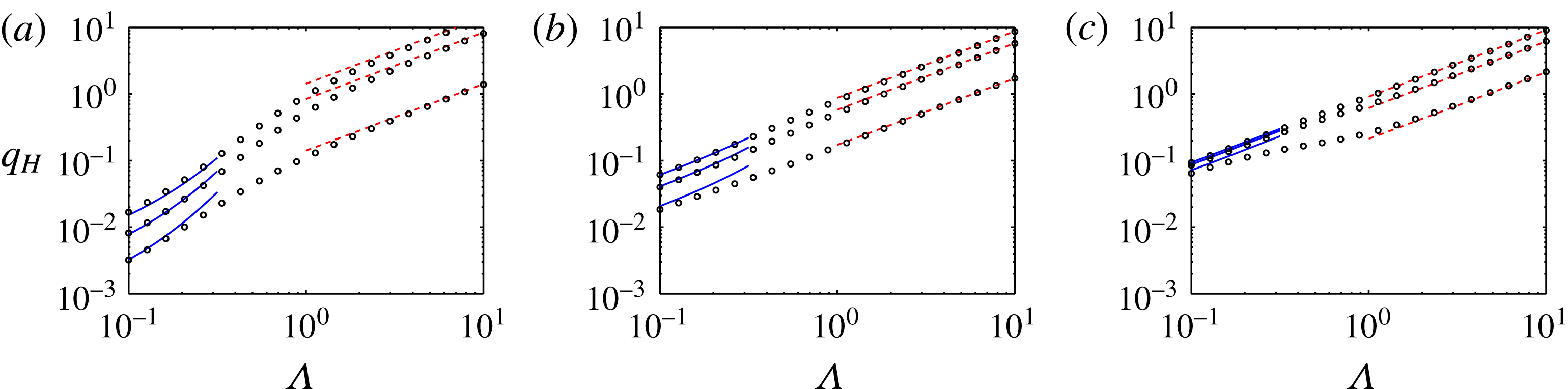
Figure 2 compares some examples of the variation of
 $q_{H}$
versus
 $\unicode[STIX]{x1D6EC}$
from the full model with the limiting cases obtained above. As the figure shows, typically as
 $\unicode[STIX]{x1D6EC}\rightarrow 10$
or
 $\unicode[STIX]{x1D6EC}\rightarrow 1/10$
, the flux functions from the full model and the limiting cases are in good agreement, implying that, as the aspect ratio approaches (or exceeds) these values, the interface general behaviours may be predicted through simple expressions, in place of heavy computations through the full model.
3.2 Flux functions and velocity fields
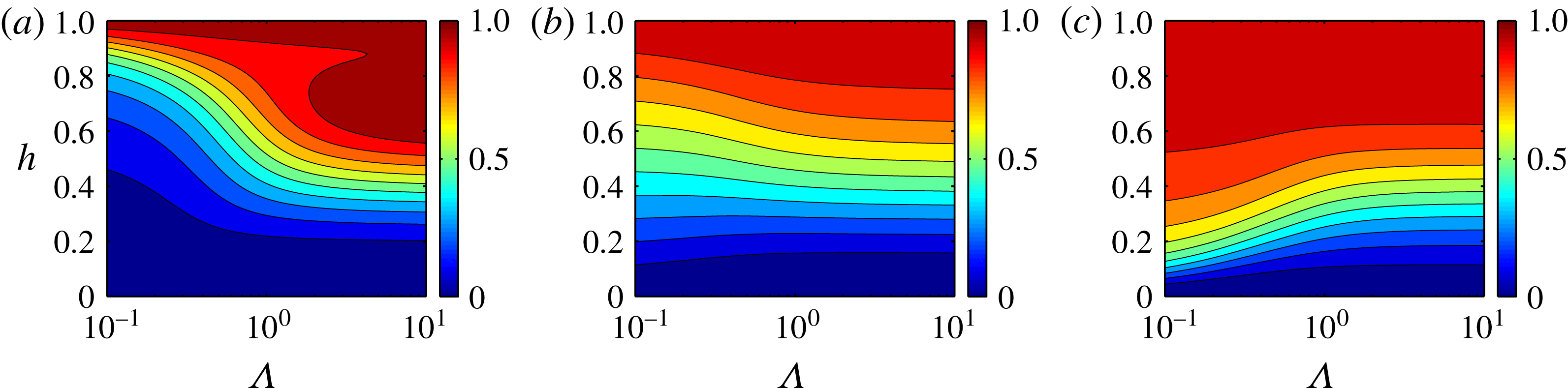
For a given set of parameters, the flux functions as well as the velocity profiles can be computed using the formulations presented. Examples of computed contours of
 $q_{H}/\unicode[STIX]{x1D6EC}$
versus
 $h$
and
 $\unicode[STIX]{x1D6EC}$
are given in figure 3. In different panels, the viscosity ratio varies. It can be seen that, for a fixed
 $\unicode[STIX]{x1D712}$
, the value of
 $q_{H}/\unicode[STIX]{x1D6EC}$
highly depends on
 $h$
,
 $m$
and
 $\unicode[STIX]{x1D6EC}$
. In particular, the viscosity ratio seems to have a strong effect on the variation of
 $q_{H}/\unicode[STIX]{x1D6EC}$
versus
 $\unicode[STIX]{x1D6EC}$
. It is also interesting to note that, for
 $m=0.1$
at moderate values of
 $\unicode[STIX]{x1D6EC}$
, the flux non-monotonically varies with
 $h$
, a feature that is not observed at small or large values of
 $\unicode[STIX]{x1D6EC}$
. Our inspection of the flux variations versus the flow parameters (not shown for brevity) also confirms that in general
 $\unicode[STIX]{x1D6EC}$
is most influential on the flux when
 $\unicode[STIX]{x1D6EC}\sim O(1)$
.
Variation of
 $q_{H}$
versus
 $\unicode[STIX]{x1D6EC}$
for
 $h_{X}=0$
(note that
 $h_{X}=\unicode[STIX]{x2202}h/\unicode[STIX]{x2202}X$
) and
 $\unicode[STIX]{x1D712}=50$
, from the full model (circles), in comparison with the limiting cases:
 $q_{H}^{\unicode[STIX]{x1D6EC}\ll 1}$
(lines) and
 $q_{H}^{\unicode[STIX]{x1D6EC}\gg 1}$
(dashed lines). From (a–c)
 $m=0.1$
,
 $m=1$
and
 $m=10$
. In each graph,
 $h=0.2$
,
 $h=0.4$
and
 $h=0.6$
from bottom to top.

Examples of contours of
 $q_{H}/\unicode[STIX]{x1D6EC}$
, versus
 $h$
and
 $\unicode[STIX]{x1D6EC}$
, for
 $\unicode[STIX]{x1D712}=30$
and
 $h_{X}=0$
. From (a–c)
 $m=0.1$
,
 $m=1$
and
 $m=10$
.

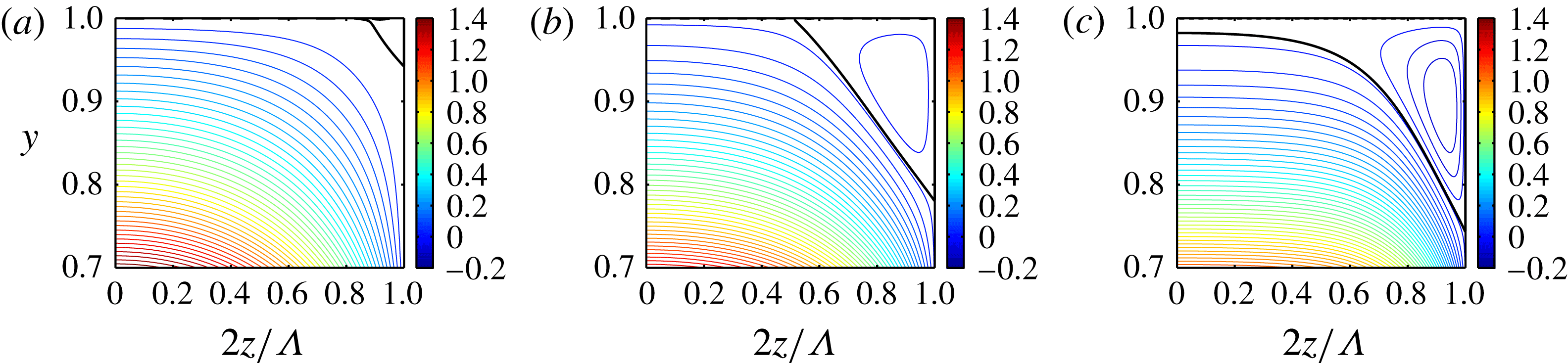
The model can be exploited to obtain the flux and velocity profiles for various ranges of the dimensionless numbers, to extract interesting information about the flow. As an example, figure 4 shows a unique feature of the rectangular channel displacement flow, which could not exist in this form in 2-D channel geometry. The velocity field contours are plotted within the rectangular channel cross-section. Note that here
 $h$
is treated as a fixed parameter and
 $\unicode[STIX]{x2202}h/\unicode[STIX]{x2202}X$
is set to zero, which are both consistent with the long-time behaviour of the interface (see § 4.2). The values above the interface are shown, meaning that they are within the displaced lighter layer. The displacement flow considered is iso-viscous. Three values of the cross-section aspect ratio are chosen along with a fixed intermediate value of the buoyancy number (i.e.
 $\unicode[STIX]{x1D712}=50$
). The thick black line in each panel corresponds to the contour line of zero velocity. In the lower side of the thick line, the velocity profiles have positive values while in the upper side of the thick line (close to the rectangle corner) the velocity profiles have negative values. This means that within the light displaced fluid and below the thick line, the displaced fluid moves forward in the direction of the mean flow while above the thick line it moves backward against the injection flow direction. It is clear from the figure that the form and the extent of the local flow reversal region depends on the value of
 $\unicode[STIX]{x1D6EC}$
.
Local flow reversal within the light fluid. Steady state velocity contours
 $u(y,z)$
versus
 $y$
and
 $2z/\unicode[STIX]{x1D6EC}$
, plotted within the light fluid within half of the duct for
 $h=0.7$
,
 $h_{X}=0$
,
 $m=1$
,
 $\unicode[STIX]{x1D712}=50$
and
 $\unicode[STIX]{x1D6EC}=1,~2,~4$
from (a–c). In each panel, the thick black line shows the zero contour line, where the light fluid velocity is zero. Below the thick line, the light fluid moves forward and above the thick line it moves backward against the mean imposed flow direction.

3.3 Numerical procedure for displacement flows
In order to obtain the motion of the interface, we need to use the kinematic condition. With regard to boundary and initial conditions, our assumptions are that the long duct is full of pure fluids
 $H$
and
 $L$
(fully developed) at the two ends of the rectangular channel and that an initially sharp profile (compatible with the far-field conditions) separates fluids
 $H$
and
 $L$
. Our simulations revealed that the propagation of the interface at longer times was not sensitive to sufficiently sharp initial interface conditions, for which a linear function in the form of
 $h(X,T=0)=-X+0.5$
was conventionally chosen. The numerical procedure was as follows. For a given set of
 $m$
,
 $\unicode[STIX]{x1D6EC}$
and
 $\unicode[STIX]{x1D712}$
, in the first time step
 $f_{H}$
and
 $f_{L}$
were calculated using the iterative method mentioned earlier and then
 $q_{H}$
was calculated through relation (3.25), subject to the initial condition. The interface evolution was then obtained using relation (3.23). In the following time steps,
 $f_{H}$
,
 $f_{L}$
and subsequently
 $q_{H}$
were calculated using
 $h$
and
 $\unicode[STIX]{x2202}h/\unicode[STIX]{x2202}X$
found in the previous time step. Regarding the discretization approach, the kinematic condition was discretized in conservative form, first order explicitly in time and second order in space, and it was integrated using on a Van Leer flux limiter scheme (Yee, Warming & Harten Reference Yee, Warming and Harten1985) for shock capturing. The convergence of the results was tested with several small spatial mesh steps (e.g.
 $\text{d}X=0.05$
, 0.1, 0.25), the choice of which showed only little effects on the interface propagation; thus,
 $\text{d}X=0.1$
was typically chosen as the mesh step. Depending on the numerical stiffness, the time step was set in the range of 0.01–0.05. Simulation results showed that the interface is always stretched out between the trailing and leading fronts. When
 $\unicode[STIX]{x1D6EC}\rightarrow \infty$
, it is expected that the results approach their 2-D channel flow counterparts. Therefore, our model results were benchmarked against those of Taghavi et al. (Reference Taghavi, Seon, Martinez and Frigaard2009) for 2-D channel displacements, finding excellent agreement.
4 Model results
Here, we present the main model results. This includes exploring the effects of the various dimensionless groups on the interface motion and the overall displacement flow.
4.1 General displacement flow behaviours based on the model
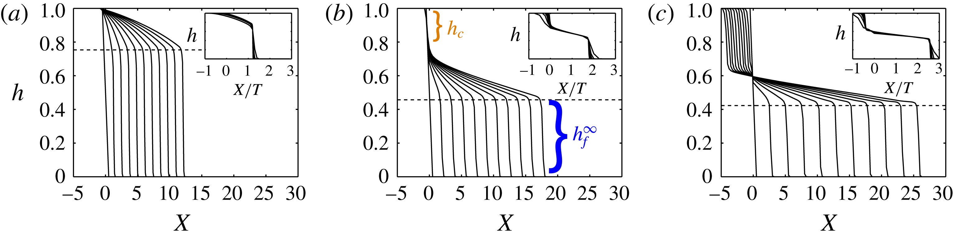
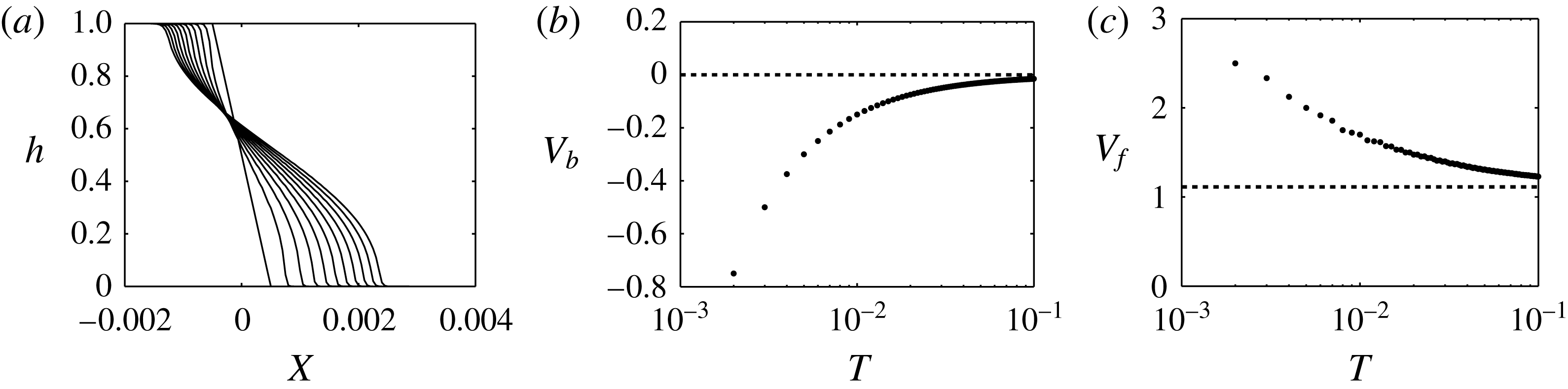
For various flow parameters, examples of displacements are plotted in figure 5. Let us first focus on figure 5(a), where a typical interface evolution with time and space is observed. The kinematic equation is solved using the sharp interface at
 $T=0$
and the interface evolution results are then plotted for ten consecutive times. For this case,
 $\unicode[STIX]{x1D6EC}=m=1$
meaning that an iso-viscous displacement occurs in a square channel geometry. In addition,
 $\unicode[STIX]{x1D712}=0$
implying that the viscous forces completely dominate the buoyancy forces that are driven by the duct slope. For the case illustrated at long times, the interface solution has two main segments, i.e. a leading front with a significant height and an interfacial segment stretched between the leading front and a trailing point, apparently pinned to the upper wall. The spatial intervals between the fronts at different times seem to be equal, implying that the front velocity must become approximately constant. The inset in figure 5(a) shows the interface height,
 $h$
, conveniently plotted against
 $X/T$
, where the interface profiles collapse onto a single similarity profile at longer times.
Examples of displacements for
 $\unicode[STIX]{x1D6EC}=m=1$
at
 $T=0,1,\ldots ,9,10$
, with
 $\unicode[STIX]{x1D712}=0,100,200$
from (a) to (c). The dashed lines illustrate the front height predictions obtained from equation (4.3) for long times. The insets show the superimposition of the interface heights at long times when plotted versus
 $X/T$
.

Comparison among the panels in figure 5 reveals the effects of increasing
 $\unicode[STIX]{x1D712}$
on the variation of the interface profiles with time. Various features can be seen. For example, due to the presence of a large buoyancy force, in figure 5(c), a trailing front with a finite (non-zero) height forms, which moves backward against the mean imposed flow direction. A comparison between figures 5(a) and 5(c) reveals the difference between a pinned trailing front (i.e. attached to the upper wall) and a moving trailing front, which usually has a considerable height. Regarding the leading front, again compared to figure 5(a), in figure 5(c) the leading front moves faster within the same time. This is simply because there exists a backflow so that the leading front needs to move relatively faster to respect the flux constraint. For an intermediate value of
 $\unicode[STIX]{x1D712}$
(carefully chosen), figure 5(b) shows a stationary interface flow state. In fact, it can be shown that for any sets of
 $\unicode[STIX]{x1D6EC}$
and
 $m$
, there exists a critical value of the buoyancy number (
 $\unicode[STIX]{x1D712}_{c}$
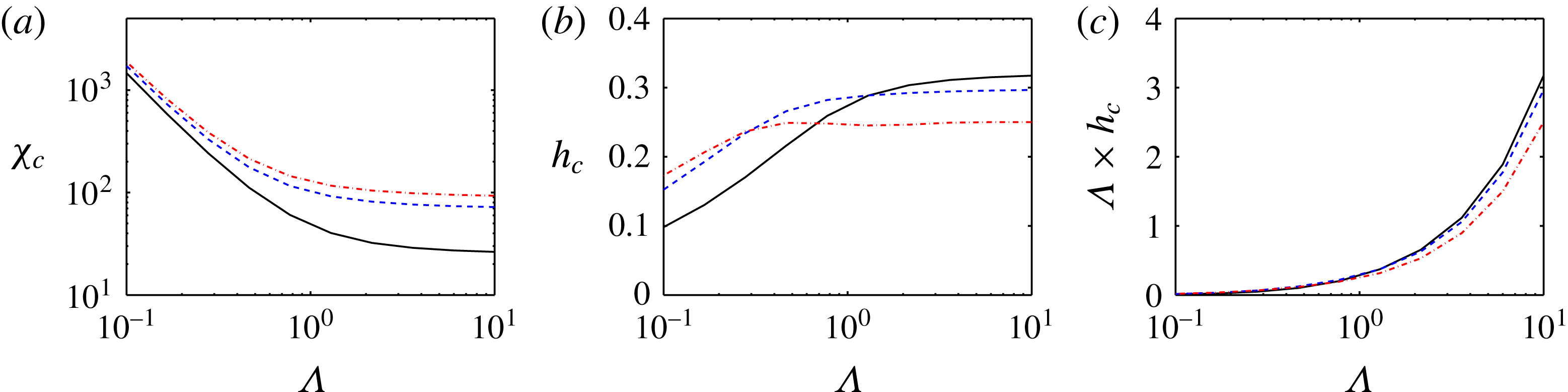
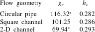
) for which there is a marginal displacement flow state with the following characteristics: (i) while the leading front is advecting from the domain, there is a significant residual layer of the light fluid that is apparently stationary; (ii) there is a critical interface height with respect to the upper wall (e.g.
 $h_{c}$
in figure 5
b) that corresponds to the thickness of a stationary layer of the displaced fluid at long times; and (iii) the trailing front is on the verge of moving upstream.
Finally, as the insets in figure 5 illustrate, the collapse of the interface profiles on a single similarity form is observed. Thus, it may be expected that the longer-time interface behaviours can be predicted more easily. Note that there is always a stretched interface segment (continuously extended as time grows), the slope of which approaches zero (in other words the interface lies parallel to the upper & lower walls). In the section below, we make use of this observation to simplify the analysis and compute the interface long-time behaviours directly, in lieu of performing simulations. This direct approach delivers, for instance, predictions to the interface height at long times (
 $h_{f}^{\infty }$
), an example of which is superimposed on figure 5(b), showing very good agreement with the simulation outcome.
We end this subsection with a flow regime classification based on the general interface characteristics observed, as
 $\unicode[STIX]{x1D712}$
decreases from a large value. Since the leading front always moves downstream regardless of the flow parameters, it is the trailing front behaviour that governs the flow regime at long times. For large values of
 $\unicode[STIX]{x1D712}$
we observe a sustained backflow where the trailing front moves continuously upward. For a critical value of
 $\unicode[STIX]{x1D712}$
, we find a stationary interface flow with the trailing front on the verge of moving upstream. Finally, for smaller values of
 $\unicode[STIX]{x1D712}$
, we encounter a no sustained backflow, where the trailing front does not move upward at long times.
4.2 Interface behaviour at long times
So far, our numerical simulations have shown that interface profiles approach a similarity form at long times. Therefore, it is appropriate to attempt to find the long-time behaviours of the interface directly, based on a few assumptions described below.
We have found that the stretched region in the interface profiles has a slope (
 $h_{X}$
) that continuously decreases as the interface elongates; accordingly, we can assume
 $h_{X}\rightarrow 0$
as
 $T\rightarrow \infty$
. Consequently, we may consider that the interface evolution at long times is governed by
 $$\begin{eqnarray}{\displaystyle \frac{\unicode[STIX]{x2202}h}{\unicode[STIX]{x2202}T}}+{\displaystyle \frac{1}{\unicode[STIX]{x1D6EC}}}{\displaystyle \frac{\unicode[STIX]{x2202}\tilde{q}_{H}}{\unicode[STIX]{x2202}X}}=0,\end{eqnarray}$$
in which
 $\tilde{q}_{H}={q_{H}|}_{h_{X}=0}$
. Meanwhile, the mass conservation of the total volume behind the interface leads to
 $\int _{0}^{1}(\unicode[STIX]{x2202}\tilde{q}_{H}/\unicode[STIX]{x2202}h)\,\text{d}h=\unicode[STIX]{x1D6EC}$
, which we use to write
 $$\begin{eqnarray}\int _{0}^{1}{\displaystyle \frac{\unicode[STIX]{x2202}\tilde{q}_{H}}{\unicode[STIX]{x2202}h}}\,\text{d}h=\unicode[STIX]{x1D6EC}V_{f}^{\infty }h_{f}^{\infty }+\int _{h_{f}^{\infty }}^{1}{\displaystyle \frac{\unicode[STIX]{x2202}\tilde{q}_{H}}{\unicode[STIX]{x2202}h}}\,\text{d}h=\unicode[STIX]{x1D6EC}\Rightarrow V_{f}^{\infty }h_{f}^{\infty }={\displaystyle \frac{\tilde{q}_{H}}{\unicode[STIX]{x1D6EC}}},\end{eqnarray}$$
in which the we can replace
 $V_{f}^{\infty }\approx 1/\unicode[STIX]{x1D6EC}(\unicode[STIX]{x2202}\tilde{q}_{H}/\unicode[STIX]{x2202}h)$
to arrive at
 $$\begin{eqnarray}{\displaystyle \frac{\unicode[STIX]{x2202}\tilde{q}_{H}}{\unicode[STIX]{x2202}h}}h_{f}^{\infty }\approx \tilde{q}_{H},\end{eqnarray}$$
where the superscript
 $\infty$
denotes the value at long times (i.e.
 $T\rightarrow \infty$
), here and elsewhere. Using the equation above, which is the underlying hyperbolic conservation law for the original parabolic problem,
 $h_{f}^{\infty }$
can be calculated using the conventional equal areas rule. The front velocity at long times,
 $V_{f}^{\infty }$
, can be then calculated straightforwardly. A similar relation can developed to predict the trailing front interface height and velocity, which we do not explain for brevity.
For the limiting case of
 $\unicode[STIX]{x1D6EC}\gg 1$
, the equations can be analytically solved to find
 $$\begin{eqnarray}{V_{f}^{\infty }|}_{\unicode[STIX]{x1D6EC}\gg 1}\approx \mathop{\sum }_{i=0}^{3}a_{i}m^{i}/\mathop{\sum }_{i=0}^{2}b_{i}m^{i},\end{eqnarray}$$
in which
 $a_{i}$
and
 $b_{i}$
, given in appendix B, are simple functions of
 $\unicode[STIX]{x1D712}$
and
 ${h_{f}^{\infty }|}_{\unicode[STIX]{x1D6EC}\gg 1}$
, which themselves are linked through
 $$\begin{eqnarray}\unicode[STIX]{x1D712}=\mathop{\sum }_{i=0}^{3}c_{i}m^{i+1}\bigg/\mathop{\sum }_{i=0}^{3}d_{i}m^{i},\end{eqnarray}$$
where
 $c_{i}$
and
 $d_{i}$
, also given in appendix B, are functions of
 ${h_{f}^{\infty }|}_{\unicode[STIX]{x1D6EC}\gg 1}$
only. For a given set of
 $(\unicode[STIX]{x1D712},m)$
,
 ${h_{f}^{\infty }|}_{\unicode[STIX]{x1D6EC}\gg 1}$
can be simply obtained through the algebraic relation (4.5) and, subsequently,
 ${V_{f}^{\infty }|}_{\unicode[STIX]{x1D6EC}\gg 1}$
can be obtained through the algebraic relation (4.4). Similar, lengthy algebraic relations can be derived for the trailing front height and velocity, which we leave for brevity.
For the limiting case of
 $\unicode[STIX]{x1D6EC}\ll 1$
, different situations may occur. First, for
 $m<1$
, there is a shock wave that can be approximated through the Rankine–Hugoniot condition (LeVeque Reference Leveque2002), revealing that
 $$\begin{eqnarray}\displaystyle & \displaystyle V_{f}^{\infty }|_{\unicode[STIX]{x1D6EC}\ll 1}^{m<1}\approx 1, & \displaystyle\end{eqnarray}$$
 $$\begin{eqnarray}\displaystyle & \displaystyle h_{f}^{\infty }|_{\unicode[STIX]{x1D6EC}\ll 1}^{m<1}\approx 1, & \displaystyle\end{eqnarray}$$
which is also approximately valid for the case of
 $m=1$
(see Zheng et al. (Reference Zheng, Guo, Christov, Celia and Stone2015a
) for the exact solution). Regarding the trailing front, as long as the effects of the channel upper wall are not neglected, the trailing front height and velocity are nearly zero. However, since
 $V_{f}^{\infty }|_{\unicode[STIX]{x1D6EC}\ll 1}^{m<1}\rightarrow 1$
and
 $h_{f}^{\infty }|_{\unicode[STIX]{x1D6EC}\ll 1}^{m<1}\rightarrow 1$
, the light fluid is effectively removed from the upper wall, implying that the flow approaches a steady travelling wave displacement for
 $m<1$
and
 $\unicode[STIX]{x1D6EC}\rightarrow 0$
.
For
 $m>1$
, the interface behaviour can be approximated by a rarefaction wave, with the interface speed in the form of
 $$\begin{eqnarray}V_{int}|_{\unicode[STIX]{x1D6EC}\ll 1}^{m>1}={\displaystyle \frac{1}{12}}{\displaystyle \frac{12m+\unicode[STIX]{x1D6EC}^{2}\unicode[STIX]{x1D712}-\unicode[STIX]{x1D6EC}^{2}\unicode[STIX]{x1D712}(m-1)h^{2}-2\unicode[STIX]{x1D6EC}^{2}\unicode[STIX]{x1D712}h}{(1+(m-1)h)^{2}}},\end{eqnarray}$$
which in the limit of
 $\unicode[STIX]{x1D6EC}\rightarrow 0$
furnishes
 $$\begin{eqnarray}\displaystyle & \displaystyle V_{f}^{\infty }|_{\unicode[STIX]{x1D6EC}\ll 1}^{m>1}\approx m, & \displaystyle\end{eqnarray}$$
 $$\begin{eqnarray}\displaystyle & \displaystyle h_{f}^{\infty }|_{\unicode[STIX]{x1D6EC}\ll 1}^{m>1}\approx 0. & \displaystyle\end{eqnarray}$$
 $$\begin{eqnarray}\displaystyle & \displaystyle V_{b}^{\infty }|_{\unicode[STIX]{x1D6EC}\ll 1}^{m>1}\approx 1/m, & \displaystyle\end{eqnarray}$$
 $$\begin{eqnarray}\displaystyle & \displaystyle h_{b}^{\infty }|_{\unicode[STIX]{x1D6EC}\ll 1}^{m>1}\approx 0. & \displaystyle\end{eqnarray}$$
For the limiting cases of
 $\unicode[STIX]{x1D6EC}\gg 1$
and
 $\unicode[STIX]{x1D6EC}\ll 1$
, the approximate solutions are provided above for the sake of comparison and completeness. A deeper analysis would fall outside the scope of the current work but an interested reader may refer to Taghavi et al. (Reference Taghavi, Seon, Martinez and Frigaard2009) and Zheng et al. (Reference Zheng, Guo, Christov, Celia and Stone2015a
,Reference Zheng, Rongy and Stone
b
) for detailed solutions of both short- and long-time flow regimes in these cases.
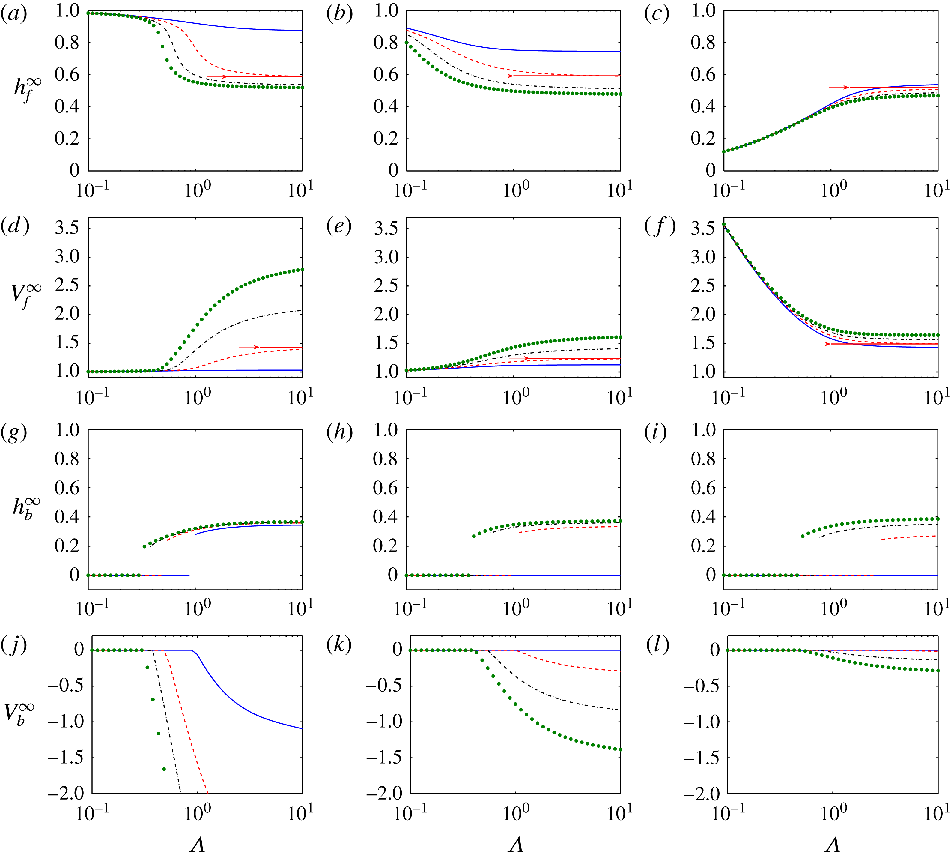
Figure 6(a–f) shows the variation of
 $h_{f}^{\infty }$
and
 $V_{f}^{\infty }$
versus
 $\unicode[STIX]{x1D6EC}$
for four typical values of the buoyancy number (within each panel) and three typical values of the viscosity ratio (in different panels within the same row). Let us first concentrate on the top row. Figure 6(a) shows that for
 $m=0.1$
, while
 $h_{f}^{\infty }$
is nearly equal to the channel height at small
 $\unicode[STIX]{x1D6EC}$
,
 $h_{f}^{\infty }$
generally decreases with increasing
 $\unicode[STIX]{x1D6EC}$
. However, it is evident that most of the front height variation occurs at the intermediate values of
 $\unicode[STIX]{x1D6EC}$
(as the cross-section aspect ratio approaches unity). For larger
 $\unicode[STIX]{x1D712}$
, the drop in
 $h_{f}^{\infty }$
is relatively more significant. Figure 6(b) for
 $m=1$
shows more or less the same trend as in figure 6(a), although the front heights are generally smaller. In contrast, figure 6(c) for
 $m=10$
shows that the front height is very small at lower values of
 $\unicode[STIX]{x1D6EC}$
but it increases rapidly with
 $\unicode[STIX]{x1D6EC}$
until
 $\unicode[STIX]{x1D6EC}\approx 1$
, after which the front height remains almost constant. The other aspect to note is that the effect of
 $\unicode[STIX]{x1D712}$
is minor for displacement flows at
 $m=10$
. Now, let us look at figure 6(d–f), showing the final front velocities that correspond to the front heights in the top row. Knowing the effects of the dimensionless parameters on the front height, their effects on the front velocity are rather expected: in general, a smaller (larger) front height implies a larger (smaller) front velocity and vice versa.
Heights and speeds of the
 $\text{leading}\backslash \text{trailing}$
fronts at long times for
 $\unicode[STIX]{x1D712}=0\backslash 50$
(solid line),
 $\unicode[STIX]{x1D712}=20\backslash 100$
(dashed line),
 $\unicode[STIX]{x1D712}=40\backslash 150$
(dash–dot line) and
 $\unicode[STIX]{x1D712}=60\backslash 200$
(dots); in each column,
 $m$
is fixed (
 $m=0.1,1,10$
from left to right). For the case of
 $\unicode[STIX]{x1D712}=20$
,
 ${V_{f}^{\infty }|}_{\unicode[STIX]{x1D6EC}\gg 1}$
and
 ${h_{f}^{\infty }|}_{\unicode[STIX]{x1D6EC}\gg 1}$
are superposed as horizontal lines (also marked by arrows).

It is logical to compare the predictions of
 $h_{f}^{\infty }$
and
 $V_{f}^{\infty }$
for the rectangular channel with those for the limiting cases discussed above. For a few cases in figure 6, the front height and velocities are compared with the corresponding values for
 $\unicode[STIX]{x1D6EC}\gg 1$
. The results show that
 $h_{f}^{\infty }$
and
 $V_{f}^{\infty }$
approach the limiting case solutions as
 $\unicode[STIX]{x1D6EC}$
increases. Several other comparisons (not shown) also confirm that the simple relations given for the limiting cases are in good agreement with the simulation results at the extreme values of
 $\unicode[STIX]{x1D6EC}$
.
Figure 6(g–i) shows the variation of the trailing front heights at long times versus
 $\unicode[STIX]{x1D6EC}$
for different values of
 $\unicode[STIX]{x1D712}$
and
 $m$
. The trailing front height is zero for small
 $\unicode[STIX]{x1D6EC}$
, but for most of the variables it goes through a significant jump as
 $\unicode[STIX]{x1D6EC}$
increases. Indeed, it is interesting to see that the trailing front, which is pinned to the upper wall for small
 $\unicode[STIX]{x1D6EC}$
, suddenly attains a significant finite height as
 $\unicode[STIX]{x1D6EC}$
approaches unity. After the jump, the variation of
 $h_{b}^{\infty }$
versus
 $\unicode[STIX]{x1D6EC}$
is not much notable, as it approaches a plateau for
 $\unicode[STIX]{x1D6EC}\gtrsim 1$
. At
 $m=10$
, for a certain value of the buoyancy number, i.e.
 $\unicode[STIX]{x1D712}=50$
, the trailing front has a height of zero (and consequently the trailing front is completely pinned to the upper wall and it neither moves upstream nor downstream) for all
 $\unicode[STIX]{x1D6EC}$
. In fact, our analysis demonstrates that the trailing front in this case is motionless for any
 $\unicode[STIX]{x1D712}\leqslant 50$
. Another aspect observed is that for larger
 $\unicode[STIX]{x1D712}$
the height of the backflow is slightly larger, although one should also consider that the ceiling value of
 $h_{b}^{\infty }$
would be
 $0.5$
, achieved at
 $\unicode[STIX]{x1D712}\rightarrow \infty$
(i.e. the exchange flow limit). Finally, if the trailing front moves upstream for a given
 $\unicode[STIX]{x1D6EC}$
, the value of the trailing front height slightly depends on
 $m$
.
Figure 6(j–l) illustrates the variation of
 $V_{b}^{\infty }$
versus
 $\unicode[STIX]{x1D6EC}$
, for different
 $\unicode[STIX]{x1D712}$
(within the same panel) and different
 $m$
(in different panels within the same row). One point to mention is that these velocities satisfy the condition
 $V_{b}^{\infty }\leqslant 0$
, implying that, if moving, the trailing front can advance only upstream against the mean imposed flow. We emphasize that no forward motion of the trailing is observed in our model simulations (unless
 $\unicode[STIX]{x1D6EC}\rightarrow 0$
). Our experiments on the other hand will show that ‘in reality’ the trailing front can move backward but also forward in some cases, perhaps due to hydrodynamic effects that are absent in our model. We will further discuss this feature in the experimental section of the current work.
Returning to analysing the behaviours of
 $V_{b}^{\infty }$
in figure 6, the trailing front velocities are zero at small
 $\unicode[STIX]{x1D6EC}$
but their absolute values start to increase when
 $\unicode[STIX]{x1D6EC}$
approaches unity. Provided that
 $h_{b}^{\infty }\neq 0$
, the trailing front becomes unpinned and it moves upstream. However, comparing the third and bottom rows, it is fairly interesting to note that
 $V_{b}^{\infty }$
does not exhibit a jump as
 $\unicode[STIX]{x1D6EC}$
increases. Instead,
 $V_{b}^{\infty }$
seems to be a continuous function of
 $\unicode[STIX]{x1D6EC}$
. Another aspect to notice is that, in contrast to the leading front, larger
 $|V_{b}^{\infty }|$
values correspond to larger
 $h_{b}^{\infty }$
values, and vice versa. This is understandable when we are reminded that the trailing front’s upward motion occurs in the act of a significant buoyancy stress to locally overcome the viscous stress induced by the imposed flow; thus, a larger buoyancy stress suggests larger
 $h_{b}^{\infty }$
and
 $V_{b}^{\infty }$
. Moreover, it is worth mentioning that, unlike the trailing front height, the trailing front velocity does not have a ceiling absolute value: relatively stronger buoyancy stresses always result in larger
 $V_{b}^{\infty }$
. Finally, as
 $m$
increases, the trailing front moves much more slowly.
 $|V_{b}^{\infty }|$
monotonically increases with
 $\unicode[STIX]{x1D6EC}$
for all
 $m$
, which was not the case for
 $V_{f}^{\infty }$
.
4.3 Multiple fronts with finite heights
Displacement flow models can be exploited to extract many displacement flow features, an example of which is the delineation of the regime boundary for multiple fronts with non-zero (finite) heights. In this context, there could be at least two types of multiple front scenarios. One is that, for a strongly buoyant flow, in addition to a leading front with a finite height (which always forms), a backflow (which is a trailing front with a finite height) may also appear. In this case, one front is moving forward (i.e. the leading front) and the other front is moving backward (i.e. the trailing front). The second scenario for the existence of multiple fronts with finite height is that for certain flow parameter sets, the interface between the two fluids may have multiple forward-moving or backward-moving fronts, appearing due to opposing effects. For instance, for a given
 $\unicode[STIX]{x1D6EC}$
, the buoyancy component driven by the duct downhill slope competes with the viscosity ratio effects between the two fluids. While the former acts to spread the interface, the latter acts to sharpen the front. Thus, when these two features are opposing each other, there is a chance for multiple forward-moving fronts to form. A second forward-moving front with a smaller speed follows the first leading front.
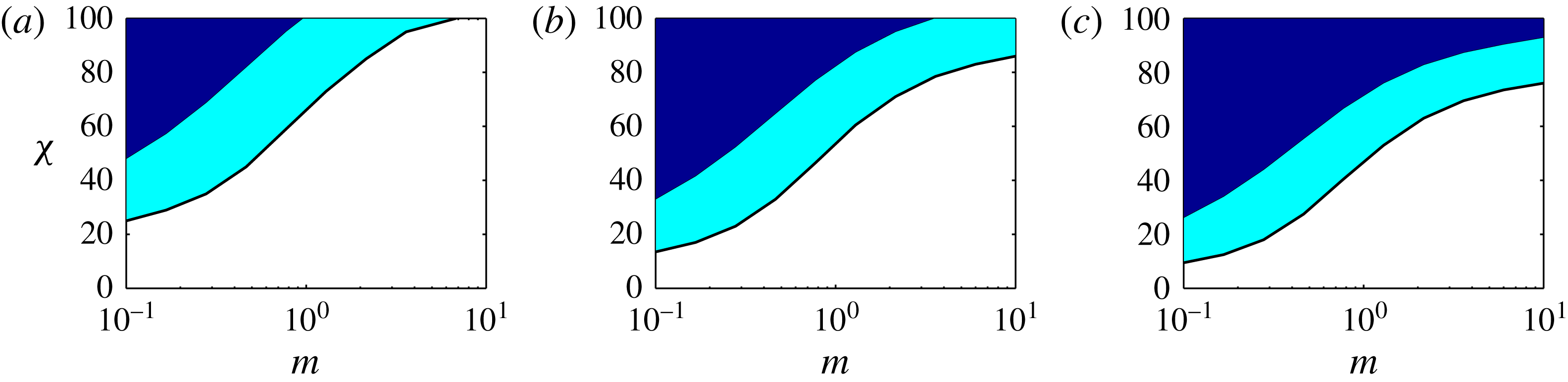
Parameter regime in the
 $(m-\unicode[STIX]{x1D712})$
-plane where multiple fronts with finite heights are marked by shaded areas. Elsewhere there is only a single leading front with a finite height and a trailing front that is pinned to the upper wall. The cross-section aspect ratio increases from (a–c)
 $\unicode[STIX]{x1D6EC}=1,2,10$
. The middle shaded area is where there exist forward-moving multiple fronts. The upper shaded area contains multiple fronts, among which at least one is a backward-moving trailing front.

Through repeated computation of
 $\tilde{q}_{H}$
for different flow parameters (
 $\unicode[STIX]{x1D6EC}$
,
 $m$
and
 $\unicode[STIX]{x1D712}$
), we can approximate the regime where multiple fronts exist, e.g. as done in figure 7, where multiple front regions are marked by the shaded areas in the plane of
 $(m-\unicode[STIX]{x1D712})$
for three different values of
 $\unicode[STIX]{x1D6EC}$
. In each panel, the non-shaded area illustrates the regime where only a single leading front with a finite height can exist. The trailing front in this case is completely pinned to the upper wall. The shaded area in the middle represents the region where there are two forward-moving leading fronts and no backward-moving trailing front. Finally, the upper shaded area marks the regime where one or more forward-moving fronts and one or more backward-moving fronts can co-exist.
4.4 Front shape
As the front propagates in a shock-like form, the frontal region itself is not a shock, but has a curved shape since diffusive effects are always present throughout the interface. In this subsection, we develop a simple approach to calculate the shape of the leading front (and similarly the trailing front) at long times. In order to do so, we first need to calculate
 $h_{f}^{\infty }$
and
 $V_{f}^{\infty }$
, using the method explained in § 4.2. Following Taghavi et al. (Reference Taghavi, Seon, Martinez and Frigaard2009) and Mollaabbasi & Taghavi (Reference Mollaabbasi and Taghavi2016) and shifting to a frame of reference that moves with the front velocity at long times,
 $\unicode[STIX]{x1D701}=X-V_{f}^{\infty }T$
, we can find a steadily travelling solution to the kinematic condition equation, which simply leads to
 $$\begin{eqnarray}{\displaystyle \frac{\text{d}}{\text{d}\unicode[STIX]{x1D701}}}\left[hV_{f}^{\infty }-{\displaystyle \frac{1}{\unicode[STIX]{x1D6EC}}}q_{H}(h,\unicode[STIX]{x1D712},h_{\unicode[STIX]{x1D701}},m,\unicode[STIX]{x1D6EC})\right]=0,\quad \Rightarrow \quad q_{H}(h,\unicode[STIX]{x1D712},h_{\unicode[STIX]{x1D701}},m,\unicode[STIX]{x1D6EC})=\unicode[STIX]{x1D6EC}hV_{f}^{\infty }.\end{eqnarray}$$
We can then solve the equation above for the interface heights that are within the interval of (
 $0,h_{f}^{\infty }$
). This in return delivers the shape of the diffusive leading front. A similar approach can be developed to obtain the shape of the diffusive trailing front, which we leave for brevity.
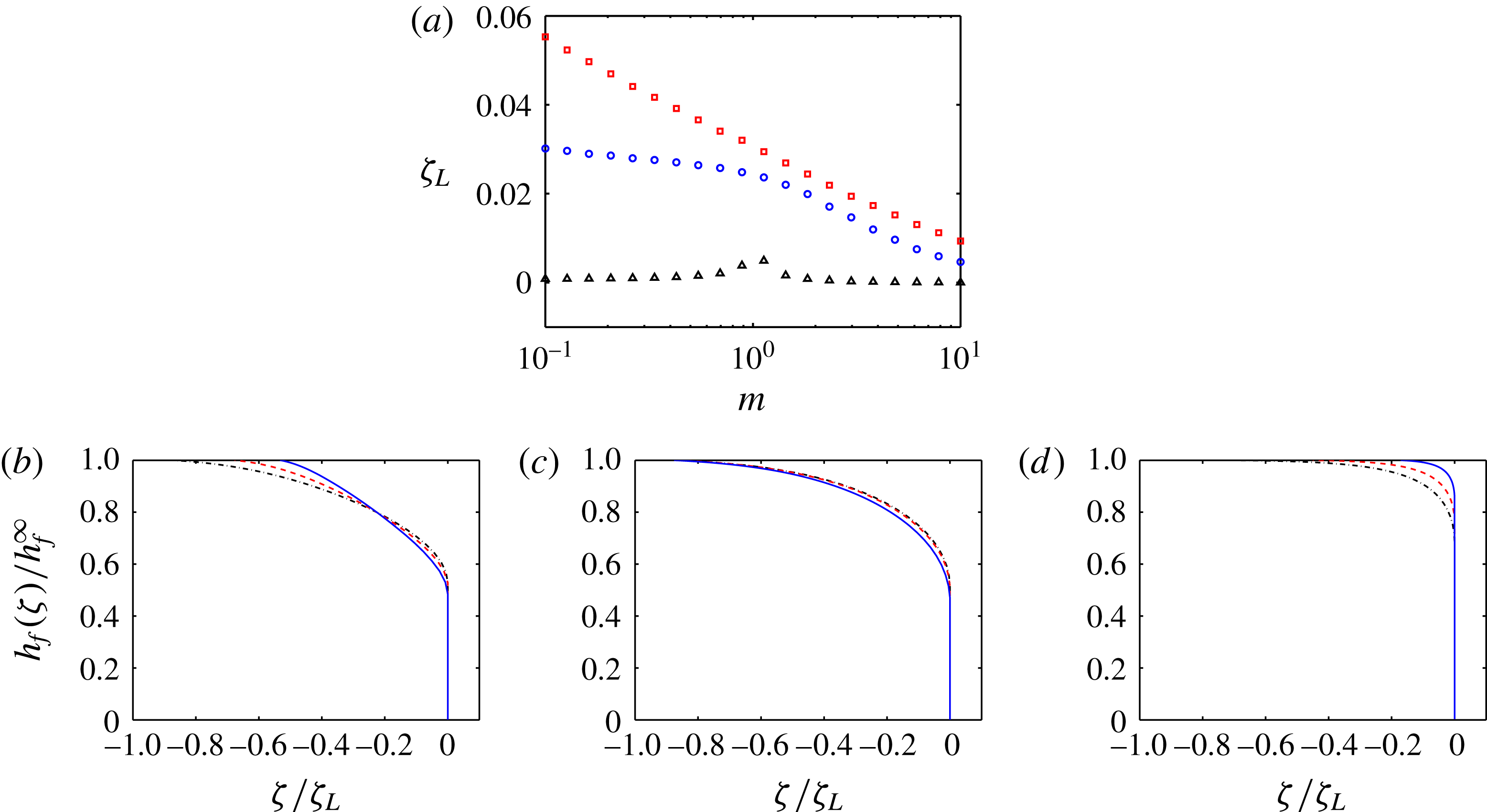
(a) Front length scale,
 $\unicode[STIX]{x1D701}_{L}$
, versus the viscosity ratio,
 $m$
, for
 $\unicode[STIX]{x1D6EC}=10$
(▫),
 $\unicode[STIX]{x1D6EC}=1$
(
 $\circ$
) and
 $\unicode[STIX]{x1D6EC}=0.1$
(▵). (b–d) Examples of the leading front shapes in the moving frame of reference at
 $\unicode[STIX]{x1D712}=0$
for
 $\unicode[STIX]{x1D6EC}=0.5$
(solid line),
 $\unicode[STIX]{x1D6EC}=1$
(dashed line) and
 $\unicode[STIX]{x1D6EC}=2$
(dash–dot line). The value of the viscosity ratio is changed in each panel:
 $m=0.1,1,10$
from left to right.

It is possible to crudely define a length scale,
 $\unicode[STIX]{x1D701}_{L}$
, over which the leading front shape varies. In order to find this length scale, we can assume that the frontal region linearly varies over
 $\unicode[STIX]{x1D701}_{L}$
, in the interval of (
 $0,h_{f}^{\infty }$
). Therefore, we can simply replace the interface slope in relation (4.13) by
 $-h_{f}^{\infty }/\unicode[STIX]{x1D701}_{L}$
and integrate to arrive at
 $$\begin{eqnarray}\displaystyle & & \displaystyle \int _{0}^{h_{f}^{\infty }}q_{H}\left(h,\unicode[STIX]{x1D712},-{\displaystyle \frac{h_{f}^{\infty }}{\unicode[STIX]{x1D701}_{L}}},m,\unicode[STIX]{x1D6EC}\right)\text{d}h\approx \int _{0}^{h_{f}^{\infty }}\unicode[STIX]{x1D6EC}hV_{f}^{\infty }\,\text{d}h={\displaystyle \frac{\unicode[STIX]{x1D6EC}V_{f}^{\infty }(h_{f}^{\infty })^{2}}{2}},\nonumber\\ \displaystyle & & \displaystyle \quad \Rightarrow \int _{0}^{h_{f}^{\infty }}q_{H}\left(h,\unicode[STIX]{x1D712},-{\displaystyle \frac{h_{f}^{\infty }}{\unicode[STIX]{x1D701}_{L}}},m,\unicode[STIX]{x1D6EC}\right)\text{d}h\approx {\displaystyle \frac{(h_{f}^{\infty })^{2}}{2}}\left.{\displaystyle \frac{\unicode[STIX]{x2202}\tilde{q}_{H}(h,\unicode[STIX]{x1D712},m,\unicode[STIX]{x1D6EC})}{\unicode[STIX]{x2202}h}}\right|_{h=h_{f}^{\infty }}.\end{eqnarray}$$
For a given parameter set (
 $\unicode[STIX]{x1D712},m,\unicode[STIX]{x1D6EC}$
), we first find
 $h_{f}^{\infty }$
through equation (4.3) and then use an iterative technique to estimate the value of
 $\unicode[STIX]{x1D701}_{L}$
that satisfies (4.14). Figure 8(a) shows the variation of
 $\unicode[STIX]{x1D701}_{L}$
versus
 $m$
, for various values of
 $\unicode[STIX]{x1D6EC}$
. We observe that
 $\unicode[STIX]{x1D701}_{L}$
significantly drops with decreasing
 $\unicode[STIX]{x1D6EC}$
. For example, at
 $\unicode[STIX]{x1D6EC}=0.1$
, the values of
 $\unicode[STIX]{x1D701}_{L}$
are quite small for different
 $m$
. In addition, for larger values of
 $\unicode[STIX]{x1D6EC}$
,
 $\unicode[STIX]{x1D701}_{L}$
gradually decreases with increasing
 $m$
.
Examples of the leading front shapes in the moving frame of reference for three values of
 $\unicode[STIX]{x1D6EC}$
and three values of
 $m$
are depicted in figure 8(b–d). For
 $m=0.1$
and
 $m=10$
, increasing
 $\unicode[STIX]{x1D6EC}$
results in the extension of the diffusive front. For
 $m=1$
, this effect is not observed. For
 $m=10$
, sharp variations in the front shape occur only when the interface height approaches
 $h_{f}^{\infty }$
.
4.5 Short-time behaviours
Since in our problem we assume that at
 $T=0$
the two fluids are put into a sudden encounter, the short-time behaviours of the interface are linked to a sharp initial interface, implying that very strong buoyancy forces are relevant. The two fluids, which are at rest initially, accelerate due to the large buoyancy while the effects of the imposed flow are not yet fully ‘felt’ by the interface. In other words, at short times, a large interface slope suggests that interface gravitational spreading dominates the imposed flow. Therefore, regardless of the flow parameters we expect that at
 $T\ll 1$
the light fluid accelerates and advances backward (against the mean imposed flow direction) and the heavy fluid accelerates and moves rapidly forward.
From the model perspective, although we are aware that at the limit of
 $T\rightarrow 0$
the model’s underlying assumptions may break down, the problem for
 $T\ll 1$
is mathematically well defined, for which the solution is worth exploring. In addition, the solution of the model at short times can deliver certain results to help gain physical insight into our flow. Moreover, our experiments will divulge that some of the real interfacial behaviours at short times are at least qualitatively in agreement with the model predictions.
Numerical solution of the short-time behaviours for
 $\unicode[STIX]{x1D6EC}=1$
,
 $\unicode[STIX]{x1D712}=0$
and
 $m=1$
. (a) Interface evolution versus time for a very sharp initial slope of the interface (
 $h_{X}=-10^{3}$
) for very short times, i.e.
 $T=[0,1,\ldots ,9,10]\times 5\times 10^{-5}$
. (b) Variation of the trailing front velocity versus time. (c) Variation of the leading front velocity versus time. The dashed lines in panels (b) and (c) show respectively the long-time leading and trailing velocities, predicted by the method explained in § 4.2.

Figure 9 shows several short-time behaviours of the interface. In order to study the early time evolution of the interface, the initial interface profile was significantly steeped. Focusing on very short times,
 $T\leqslant 5\times 10^{-4}$
, figure 9(a) shows the evolution of the interface with time. Due to the steepness of the initial interface, the buoyancy stress is locally large, which leads to a momentarily backflow behaviour: the trailing front moves backward, but it eventually stops (and becomes nearly pinned). Figure 9(b) shows that the absolute value of the trailing front velocity decreases as time grows and
 $V_{b}$
asymptotically approaches
 $V_{b}^{\infty }$
, i.e. zero in this case (thus, a no-sustained-backflow regime is observed at long times). The decrease in
 $|V_{b}^{\infty }|$
is due to the fact that the interface is stretched and its ‘average’ slope deceases, implying that the overall buoyancy force decreases. In this case, at long times, the buoyancy component induced by the downhill slope is zero (
 $\unicode[STIX]{x1D712}=0$
, e.g. the duct can be considered horizontal) and therefore the trailing front eventually stops close to its initial encounter position. Similarly, the large buoyancy force causes the leading front to move faster so that
 $V_{f}$
is initially larger, as shown in figure 9(c). However,
 $V_{f}$
gradually decreases. Similar to the trailing front, the leading front velocity quickly approaches
 $V_{f}^{\infty }$
.
Before we proceed, it is worth further emphasizing the transition between exchange-like to displacement-like flows. First, in the limiting case of
 $\unicode[STIX]{x1D712}\gg 1$
, one may expect to recover the diffusive spreading of the interface, similar to classical exchange flows. In our case, as the interface spreads, the pressure gradient due to the imposed flow rate and the buoyancy term coming from the inclination angle are constant, while the buoyancy force due to the interface slope decreases rapidly and becomes negligible. In other words, there is a rapid transition from a ‘diffusive’ to a ‘convective’ regime. For the case of a 2-D channel displacement flow, this transition has been thoroughly discussed and quantified in Taghavi et al. (Reference Taghavi, Seon, Martinez and Frigaard2009).
4.6 Critical stationary interface flows
We have observed from our numerical simulations that for a critical value of
 $\unicode[STIX]{x1D712}$
, we find a marginal stationary interface flow state. In this subsection, we provide a method to predict this critical state, which is of great physical and practical interest since the stationary interface state characterizes the transition between the sustained-backflow and no-sustained-backflow regimes.
In the view of our model, a few considerations can help identify stationary interface flows. First of all, these flows are observed at long times when the interface is elongated. Second, the thickness of the displaced layer is finite (non-zero) and typically significant with respect to the channel height. Third, the flow rate of the heavy displacing fluid is constant. Therefore, from our model perspective, a stationary residual layer of the displacement fluid is equivalent to an interfacial speed of zero and the flux equal to
 $\unicode[STIX]{x1D6EC}$
at the interface. As observed earlier in our simulations, the interfacial slope is negligible throughout the elongated region of the interface, so that
 $h_{X}$
can be simply set to zero. Therefore, to obtain the stationary interface state, we can write
 $$\begin{eqnarray}\displaystyle & \displaystyle \tilde{q}_{H}(1-h_{c},\unicode[STIX]{x1D712}_{c},m,\unicode[STIX]{x1D6EC})=\unicode[STIX]{x1D6EC}, & \displaystyle\end{eqnarray}$$
 $$\begin{eqnarray}\displaystyle & \displaystyle \left.{\displaystyle \frac{\unicode[STIX]{x2202}\tilde{q}_{H}(h,\unicode[STIX]{x1D712}_{c},m,\unicode[STIX]{x1D6EC})}{\unicode[STIX]{x2202}h}}\right|_{h=1-h_{c}}=0, & \displaystyle\end{eqnarray}$$
where
 $\unicode[STIX]{x1D712}_{c}$
denotes the critical value of the buoyancy number and
 $h_{c}$
denotes the critical height (thickness) of the residual layer, measured from the upper wall. Solving the coupled equations above, we can find the values of
 $h_{c}$
and
 $\unicode[STIX]{x1D712}_{c}$
for a given set of
 $\unicode[STIX]{x1D6EC}$
and
 $m$
. Note that the leading front height can also be calculated for stationary interface flows; however, its value would be of much less interest since for a sufficiently elongated interface the effect of the front height on the stationary layer is insignificant.
Figure 10(a) shows the variation of
 $\unicode[STIX]{x1D712}_{c}$
versus
 $\unicode[STIX]{x1D6EC}$
, for various
 $m$
. First of all,
 $\unicode[STIX]{x1D712}_{c}$
decreases with
 $\unicode[STIX]{x1D6EC}$
, which may be intuitive since by increasing
 $\unicode[STIX]{x1D6EC}$
the total buoyancy force in the cross-section increases and therefore the critical value of
 $\unicode[STIX]{x1D712}$
required for the stationary interface condition decreases. However, for
 $\unicode[STIX]{x1D6EC}>1$
a plateau is reached. Moreover, by increasing the viscosity ratio,
 $\unicode[STIX]{x1D712}_{c}$
monotonically increases. Figure 10(b) plots the variation of
 $h_{c}$
versus
 $\unicode[STIX]{x1D6EC}$
, where
 $h_{c}$
increases rapidly but it reaches almost a plateau for
 $\unicode[STIX]{x1D6EC}>1$
. Although a monotonic behaviour may be expected beforehand for the effect of
 $\unicode[STIX]{x1D6EC}$
on
 $h_{c}$
, the effect of
 $m$
is not a priori known. In fact, the variation of
 $h_{c}$
with
 $m$
is non-monotonic: at small
 $\unicode[STIX]{x1D6EC}$
, increasing
 $m$
results in a larger
 $h_{c}$
, while at large
 $\unicode[STIX]{x1D6EC}$
increasing
 $m$
results in a smaller
 $h_{c}$
. As
 $\unicode[STIX]{x1D6EC}$
increases, figure 10(c) shows the variation of
 $\unicode[STIX]{x1D6EC}\times h_{c}$
, which is the transverse area left stationary. The new parameter used, i.e.
 $\unicode[STIX]{x1D6EC}\times h_{c}$
, can be also interpreted as the stationary layer volume per unit length of the duct. In general, the displaced fluid volume that is left behind stationary increases with
 $\unicode[STIX]{x1D6EC}$
and
 $m$
.
Variation of critical values versus
 $\unicode[STIX]{x1D6EC}$
, for the stationary flow state, for
 $m=0.1$
(solid line),
 $m=1$
(dashed line) and
 $m=10$
(dash–dot line).

Comparison of the critical values for the stationary interface condition, for two-layer displacements in typical flow geometries. The values of the critical buoyancy number (
 $\unicode[STIX]{x1D712}_{c}$
) and the stationary layer thickness (
 $h_{c}$
) are given for iso-viscous displacement flows (
 $m=1$
) in near-horizontal inclinations. The values marked by ‘
 $\ast$
’ are taken from Taghavi et al. (Reference Taghavi, Seon, Wielage-Burchard, Martinez and Frigaard2011). In the definition of
 $\unicode[STIX]{x1D712}$
for different geometries, the pipe diameter or channel height has been used as the characteristic length scale.

One of the contributions of the current study could be shedding light on the effects of rectangular channel flow geometry on various displacement flow features, compared to other flow geometries, for which we present an example here. Table 1 shows the values of
 $\unicode[STIX]{x1D712}_{c}$
and
 $h_{c}$
for various typical displacement flow geometries. It is curious to see that while the thickness of the critical stationary layers are very close to each other for these flow geometries, the values of
 $\unicode[STIX]{x1D712}_{c}$
are fairly different. The highest
 $\unicode[STIX]{x1D712}_{c}$
belongs to the circular pipe, whereas the lowest
 $\unicode[STIX]{x1D712}_{c}$
belongs to the 2-D channel. The critical buoyancy number of the square channel flow is in the middle. For fixed fluid properties, as the buoyancy number increases, a smaller
 $\unicode[STIX]{x1D712}_{c}$
value suggests that a larger imposed flow is needed to achieve the stationary interface condition. Therefore, the trend observed may be justifiable. Loosely speaking, for a 2-D channel flow, there are less restrictive walls compared to the square and circular pipe flows; thus, for the same parameters the viscous resistance is weaker and the buoyancy force is relatively stronger in the 2-D channel, resulting in the smallest
 $\unicode[STIX]{x1D712}_{c}$
required to achieve the stationary interface condition. Note that table 1 provides just one example of an insightful comparison that can be made. Several similar comparisons can be also carried out, e.g. to obtain
 $\unicode[STIX]{x1D712}_{c}$
and
 $h_{c}$
in different flow geometries for displacements with various viscosity ratios.
Due to its practical importance, quantifying
 $\unicode[STIX]{x1D712}_{c}$
for various flows has received recent attention. For example, using a lattice Boltzmann method, Redapangu, Sahu & Vanka (Reference Redapangu, Sahu and Vanka2012) performed displacement flow simulations of two immiscible fluids in an inclined channel while considering the effects of viscosity and density contrasts. Among several relevant results (e.g. quantifying the leading/trailing front velocities), their simulations also revealed that the value of the critical buoyancy number of their case was
 $\unicode[STIX]{x1D712}_{c}=193.6$
, which is larger than the value reported by Taghavi et al. (Reference Taghavi, Seon, Wielage-Burchard, Martinez and Frigaard2011) (i.e.
 $\unicode[STIX]{x1D712}_{c}=69.94$
) for the miscible counterpart.
5 Experiment
In order to complement our theoretical work, we have performed a large number of displacement flow experiments, which we analyse in this section. Our main goal is to draw a comparison between the model and experiments, in order to understand the domains of the validity of the model and delineate its strengths and limits in capturing various physical phenomena. The model developed included three key dimensionless parameters, i.e. a buoyancy number, the viscosity ratio and the cross-section aspect ratio. However, since covering all the parametric regimes is evidently not feasible in a single experimental study, we will treat
 $m$
and
 $\unicode[STIX]{x1D6EC}$
as constant parameters in our experiments.
5.1 Experimental descriptions
Our experiments were performed in a
 $2450$
mm long, transparent duct (acrylic with
 ${\sim}1.5$
mm thickness) with a nearly square shape cross-section (
 $\hat{D}_{0}=$
15.65 mm and
 $\hat{D}_{00}=$
15.85 mm
 $\Rightarrow$
 $\unicode[STIX]{x1D6EC}\approx 1.013$
), as depicted schematically in figure 11(a). The duct was mounted on a robust frame that could be tilted at a desired angle. An automated, pneumatic mini gate valve (VAT, Inc.) located 716 mm from the duct inlet was included in the flow loop. The gate valve role was to initially separate the two parts of the duct, to completely segregate the displacing and displaced fluids. The valve system was designed in a way that it could be instantaneously opened at the beginning of each experiment.
Initially, the duct section above the gate valve was filled with a denser fluid (i.e. sodium chloride–water solution), while the lower section was filled with a less dense fluid (i.e. pure water). For visualization purposes, the light fluid was coloured with a small amount of ink (Fountain Pen India black ink). Fluid densities were measured by a high-precision density meter (Anton Paar DMA 35). Fluid viscosities were measured using a digital controlled shear stress-shear rate rheometer (AR-G2 TA Instrument), revealing that at the salt concentrations of our interest the fluids were Newtonian and that their viscosities remained very close to that of pure water. Thus, any small variation of the viscosity due to the salt presence was neglected and a common, constant kinematic viscosity was considered for both displaced and displacing fluids, i.e.
 $\unicode[STIX]{x1D708}=10^{-6}~\text{m}^{2}~\text{s}^{-1}$
. Ambient temperature was kept at
 $24\pm 1$
 $^{\circ }\text{C}$
for all the experiments.
In order to avoid pump disturbances, the displacing heavier fluid was fed by gravity from a large elevated tank. This allowed to ensure smooth, steady inflow and also avoid any bubble formations in the duct, which would have distorted the experimental data. The imposed flow rate for each experiment was controlled by a needle valve and measured with a turbine flowmeter (FTB-420, Omega), with an accuracy of
 $\pm 3\,\%$
. The flow rate along with the other measurements were transferred to a computer through an acquisition card (model USB-6002, National Instruments).
Panel (a) shows a schematic view of our experimental apparatus. Panels (b–f) show the results for experiment
 $VI$
. (b) Image sequence showing the evolution of a typical displacement. From top to bottom are shown images for
 $\hat{t}=1.8,3.6,\ldots ,16.2,18$
s. The field of view is
 $2450\times 12.5~\text{mm}^{2}$
. (c) The extracted experimental interface evolution, for the same times as in panel (b). The inset shows the collapse of
 $h$
when plotted versus
 $x/t$
. Horizontal dashed lines mark the front height at long times. (d) Variation of the leading front velocity with time. Dashed line shows
 $\hat{V}_{f}^{\infty }=93~\text{mm}~\text{s}^{-1}$
. (e) Velocity contour results
 $(\text{mm}~\text{s}^{-1})$
at the UDV probe positions in line with the
 $\hat{z}$
-axis fixed at
 $(\hat{x},{\hat{y}})\approx (894,16)$
(mm). From top to bottom the velocity contours correspond to
 $\hat{z}\approx -4,~0,+4$
(mm). (f) Velocity contour results (
 $\text{mm}~\text{s}^{-1}$
) at the UDV probe positions in line with the
 ${\hat{y}}$
-axis fixed at
 $(\hat{x},\hat{z})\approx (894,8)$
(mm). From top to bottom the velocity contours correspond to
 ${\hat{y}}\approx 4,~8,~12$
mm. Velocity contours are averaged in time over several consecutive velocity profiles.

The images were taken using a monochromatic camera (Basler acA2040, with 4096 grey scale levels), covering almost the entire length of the duct. Depending on the mean imposed flow velocity value, the images were recorded at a frame rate varying between 2 f.p.s. and 10 f.p.s. After post-processing using in-house Matlab codes, these series of images allowed to produce spatio-temporal representations for each experiment and study the flow large-scale features, e.g. interfacial behaviours. To have a uniform lighting across the duct, light-emitting diodes were placed behind the duct and diffusive panels were placed in between. Light absorption calibrations were performed in usual fashion. For instance, before each experiment, an image of the duct containing the transparent, heavier solution and an image of the duct containing the darker, lighter solution were recorded, which served as references of light intensities for the Beer–Lambert law.
For certain experiments, we used an ultrasonic Doppler velocimeter (UDV) (DOP4000, Signal-Processing) to measure the velocity profiles within the displacing and displaced fluids. Polyacrylamide powder with concentration equal to
 $0.2~\text{g}~\text{l}^{-1}$
was added to both solutions to amplify the measurements of the profiles. The velocity profiles (projections) were usually measured at 849 mm below the gate valve, which is nearly in the middle of duct section downstream.
Dimensional and dimensionless experimental parameters (
 $\unicode[STIX]{x1D712}$
varies in the range 0–7082). The two fluids are (nearly) iso-viscous with
 $\hat{\unicode[STIX]{x1D708}}\approx 1~\text{mm}^{2}~\text{s}^{-1}$
as the common kinematic viscosity; therefore,
 $m\approx 1$
. All the experiments are performed in a nearly square duct, with the cross-section area of
 $15.65\times 15.85$
mm
 $^{2}$
; therefore,
 $\unicode[STIX]{x1D6EC}\approx 1.013$
is fixed in our experiments. Certain experiments labelled by Roman numerals will be referenced in the following figures.

More than 220 iso-viscous displacement experiments were performed in the nearly square duct, for a wide range of imposed flow velocities and density differences. Table 2 shows the ranges over which the experiments were conducted. As can be seen, the duct inclination angles were kept close to horizontal (i.e.
 $\unicode[STIX]{x1D6FD}\geqslant 82^{\circ }$
) while the densities were also close to each other, to respect the Boussinesq approximation. The ranges of the dimensionless parameters are also given in the table, from which it is clear that our experiments cover a wide range.
5.2 General displacement flow observations
In our experiments, the displacement always starts with both fluids at rest. Therefore, when the gate valve is opened, the two fluids accelerate quickly over a few seconds. The static head pushes the fluids towards the duct outlet, generating a mean imposed velocity. Meanwhile the buoyancy force, caused by the density difference between the two fluids, accelerates the displacing and displaced fluid in the opposite directions.
Similar to our model, the initial interface (at time equal to zero) is transverse to the duct longitudinal axis. However, unlike our model where inertia is absent, in our experiment inertia remains a key force to balance the buoyancy force at very short times. As the displacement evolves and the interface stretches, at some point of time, the overall slope of the interface relative to the slope of the ducts becomes sufficiently reduced in a manner that the viscous force can become the principal player in balancing the buoyancy force. Although the extremely short-time behaviours could be of interest, in this paper we will take no further notice of the initial phase and concentrate on analysing the displacement flow longer-time dynamics.
At longer times, the general qualitative flow behaviours are similar to our model observations. As the displacement develops, typically two fronts appear: a leading front that is towards the bottom of the duct and a trailing front that is towards to its top. The interface between these fronts is stretched axially along the duct. In the following sections, we will study the characteristics of the leading/trailing fronts in our experiments, and analyse their similarities & differences in comparison with those predicted by the model.
Figure 11 shows an ensemble of panels to clarify our experimental approach and typical results. Figure 11(a) shows a schematic view of the experimental apparatus, i.e. a long duct, as discussed earlier. The position of the gate valve (in close and open conditions) is depicted. The camera is parallel to the
 $\hat{z}$
-axis so that it delivers 2-D images of the ducts in the
 $\hat{x}$
–
 ${\hat{y}}$
plane. Six UDV probe positions typically used in our experiments are also depicted in the schematic. These UDV probes provide the velocity profiles (projections) along different vertical or horizontal imaginary lines that pass perpendicularly through the duct cross-section.
Figure 11(b) shows the image sequence for a typical experiment. Figure 11(c) illustrates the interface evolution with time and space, showing that it evolves smoothly and stably. The inset of figure 11(c) shows that at long times the interfaces are superposed if
 $h$
is plotted against
 $x/t$
, suggesting that the interfaces become almost self-similar and that the front speed becomes nearly constant at longer times. These two features were also observed in the model results. Figure 11(d) shows an example where the variation of the leading front speed (accumulative) is plotted against time. Note that in order to reduce the near-wall noises in analysing front velocities, the interfacial leading and trailing front velocities were estimated at
 $h=0.1$
and
 $h=0.9$
, respectively. Figure 11(d) shows that the leading front velocity rapidly increases and reaches its nearly steady limit at long times, i.e.
 $\hat{V}_{f}^{\infty }$
. It is possible to further analyse the variation of
 $\hat{V}_{f}$
versus
 $\hat{t}$
to obtain the characteristic time over which the leading front accelerates, which we leave to future works.
Figure 11(e,f) shows the velocity contours versus
 ${\hat{y}}$
–
 $\hat{t}$
and
 $\hat{z}$
–
 $\hat{t}$
, respectively. Note that in figure 11(e,f) each panel contains three different contour plots. These panels suggest that more or less at
 $\hat{t}\approx 10$
(s) the leading front reaches the vicinity of the probes. Figure 11(e) shows that the displacing layer velocity close to the middle/sides of the duct (in the
 $\hat{x}$
–
 ${\hat{y}}$
plane) is expectedly larger/smaller. Figure 11(e) also shows that the displaced layer initially has a larger velocity, which decreases as the leading front passes by the probe positions. The explanation for this behaviour is simple: in a single-layer fluid there is no buoyancy effect, whereas buoyancy in a two-layer flow acts on the displaced layer to resist against the mean imposed flow, reducing its velocity. Figure 11(f) illustrates that, intuitively, the flow velocity close to the middle of the duct (
 $\hat{x}$
–
 $\hat{z}$
plane) is relatively larger. Finally, although the generally smooth contours in figure 11(e) imply that the overall flow must be laminar, there are small fluctuations observed in the flow velocity contours of figure 11(f), suggesting that there are still non-negligible inertial effects in our displacement flows. As will be seen, inertial effects can modify certain interfacial behaviours, including front velocities.
Before proceeding, we note that many of our general observations are in qualitative agreement with the literature considering relevant flows. In particular, we have compared our results with those of Taghavi et al. (Reference Taghavi, Alba, Seon, Wielage-Burchard, Martinez and Frigaard2012b ), who have experimentally studied buoyant displacement flows in pipes, finding that, for comparable flow parameters, the overall flow behaviours (e.g. interface evolution, formation of leading/trailing fronts, etc.) are quite similar. In addition, we have carried out qualitative comparisons with the results of Sahu et al. (Reference Sahu, Ding, Valluri and Matar2009a ,Reference Sahu, Ding, Valluri and Matar b ), who have studied buoyant displacement flows of two miscible fluids in 2-D inclined channels via direct numerical simulations of the Navier–Stokes equations. Analogous to our observations, Sahu et al. (Reference Sahu, Ding, Valluri and Matar2009a ) have found that in close to horizontal inclinations the fluids are clearly segregated, even at significant inertia and buoyancy. Another agreement with the findings of Sahu et al. (Reference Sahu, Ding, Valluri and Matar2009a ) is that by increasing the inclination angle or the density ratio the leading front velocity increases. Another common observation is that by increasing the inclination angle, inertial effects become stronger and instabilities may grow.
5.3 Viscous and inertial flows
As expected, at near-horizontal inclinations we observe that the displacement in the majority of our experiments remains viscous with no sign of instability or interfacial waves at long times. However, in some cases (e.g. the largest inclination from horizontal and the largest
 $At$
), there exist flow instabilities, interfacial waves and partial mixing between the two fluids. Our aim in this work is neither to study inertial flows nor to exactly delineate the transition between viscous and inertial flows. However, before we proceed, it is favourable to emphasize that for inclinations and density differences larger than those presented in our study, inertial effects can become dominant. This in return justifies the reason for the experimental parameter ranges chosen and also imposes an obvious boundary to the range of the relevance of the theoretical model.
It is expected that, as the inclination and/or the density difference between the two fluids increase, the inertial effects become progressively more present. Based on the image sequences and spatio-temporal diagrams, it is possible to crudely distinguish between inertial and viscous flow regimes based on the following criteria: we define viscous fluids as those that remain primarily laminarized and unidirectional, with a clean interface and no evidence of instability (on the image sequences or spatio-temporal diagrams). On the other hand, we refer to inertial flows when there is evidence of two- and three-dimensional flows, typically associated with instability and localized mixing close to the interface.
Experimental datapoints marking viscous flows (●) and inertial flows (▫). Examples of spatio-temporal diagrams obtained for experiments
 $V$
and
 $VII$
are plotted as lower and upper insets, respectively. Dashed line marks the transition boundary using equation (5.1) for
 $h_{s}=0.6$
.

Based on the definitions presented, figure 12 shows datapoints belonging to viscous and inertial flows. As can be seen, the majority of the datapoints belong to viscous displacement flows. However, there exist a number of experiments showing significant inertial effects. Two insets are added to the figure, which depict the spatio-temporal diagrams of the averaged concentration profiles along the length of the duct. The leading front can be recognized on each diagram through a sharp boundary between the different relative concentrations of the heavy and light fluids. In addition, the behaviours of the interface, such as appearance of waves and instabilities (if any), can be clearly observed on these types of diagrams. The lower inset refers to an inertial datapoint, where waves appear at the interface between the two fluids. The speed of these waves can be extracted through the slope of the contrasts in the diagram. On the other hand, the upper inset shows a viscous datapoint (marked by the arrow). With respect to the inertial datapoint, the only difference is that the mean imposed velocity has increased, which stabilizes the flow and results in a ‘clean’ spatio-temporal diagram with no evidence of interfacial wave/instability. This counter-intuitive effect, i.e. stabilizing a confined buoyant flow by increasing the mean imposed flow velocity, has been extensively studied in recent years, e.g. in Taghavi et al. (Reference Taghavi, Seon, Wielage-Burchard, Martinez and Frigaard2011) and Amiri, Larachi & Taghavi (Reference Amiri, Larachi and Taghavi2016).
Experimentally,
 $\unicode[STIX]{x1D712}$
and
 $\unicode[STIX]{x1D6FF}Re$
are the main dimensionless parameters of the flow and one may expect that plotting the datapoints using these dimensionless groups may separate inertial and viscous flows, which is approximately the case in figure 12. However, even the large number of our experimental datapoints is not sufficient to allow to exactly delineate the transition boundary between the two flow regimes. Perhaps in a future work, the stability analysis of displacement flows in rectangular channels can be performed to deliver the critical boundary that separates the viscous and inertial regimes. To motivate such future study and demonstrate that such analysis may be useful, on this graph we have superimposed the transition boundary for an inclined 2-D channel displacement, found through a long wavelength stability analysis (Taghavi et al.
Reference Taghavi, Alba, Seon, Wielage-Burchard, Martinez and Frigaard2012b
):
 $$\begin{eqnarray}\unicode[STIX]{x1D6FF}Re={\displaystyle \frac{140}{\unicode[STIX]{x1D712}[3(2h_{s}-1)(33h_{s}^{2}-33+2)-\unicode[STIX]{x1D712}h_{s}^{2}(1-h_{s})(73h_{s}^{3}-146h_{s}^{2}+92h_{s}-19)]}}.\end{eqnarray}$$
The dashed line in figure 12 shows the critical
 $\unicode[STIX]{x1D6FF}Re$
as a function of
 $\unicode[STIX]{x1D712}$
for a given steady interface height (
 $h_{s}$
). A fixed value of
 $h_{s}=0.6$
, as a representative average interface height, has been used to draw the dashed line. As expected, the critical transition dashed line (i.e. appropriate for 2-D channel flows) does not completely match our case, which is expected as here we deal with a square channel flow rather than a 2-D channel flow. Nevertheless, the trend seems quite reasonable, which may motivate the development of a rigorous stability analysis, e.g. through long wavelength weighted residual approaches (e.g. Amaouche, Mehidi & Amatousse Reference Amaouche, Mehidi and Amatousse2007; Alba, Taghavi & Frigaard Reference Alba, Taghavi and Frigaard2013b
). In fact, since the stability of the flows of our interest cannot generally be determined beforehand, model simplifications such as the one presented in this work can be utilized so that the study of the stability problem becomes possible in future.
Before we proceed, it is reasonable to make a link between the instabilities arising in our flows and those extensively studied in the literature (see Govindarajan & Sahu (Reference Govindarajan and Sahu2014) for an appealing review). Among several types of instabilities in the context of miscible multi-layer flows, those studied by Sahu et al. (Reference Sahu, Ding, Valluri and Matar2009a ) seem pertinent to our work. For plane channel geometry and miscible fluids, their linear stability analysis and numerical simulations demonstrated that, in the presence of a density difference, the instabilities are of Kelvin–Helmholtz type, leading to ‘roll-up’ structures. For buoyant displacement flows in pipes, Taghavi et al. (Reference Taghavi, Alba, Seon, Wielage-Burchard, Martinez and Frigaard2012b ) confirmed this picture experimentally. To the best of our knowledge, the stability of buoyant miscible displacement flows in rectangular channels has not been analysed, although there are relevant works for the immiscible counterparts, e.g. Redapangu et al. (Reference Redapangu, Sahu and Vanka2013) who found screw type instabilities, exclusively observed in 3-D channels.
5.4 Leading front behaviours
Comparison between the leading front velocities obtained from the model and experiments. Datapoints correspond to experiments performed at
 $At=10^{-3}$
with
 $\unicode[STIX]{x1D6FD}=90^{\circ }$
(▪),
 $\unicode[STIX]{x1D6FD}=88^{\circ }$
(▴),
 $\unicode[STIX]{x1D6FD}=85^{\circ }$
(●) and
 $\unicode[STIX]{x1D6FD}=88^{\circ }$
(
 $\star$
);
 $At=5\times 10^{-3}$
with
 $\unicode[STIX]{x1D6FD}=90^{\circ }$
(
 $\times$
),
 $\unicode[STIX]{x1D6FD}=88^{\circ }$
(
 $+$
),
 $\unicode[STIX]{x1D6FD}=85^{\circ }$
(
 $\ast$
) and
 $\unicode[STIX]{x1D6FD}=82^{\circ }$
(

 $At=10^{-2}$
with
 $\unicode[STIX]{x1D6FD}=90^{\circ }$
(▾),
 $\unicode[STIX]{x1D6FD}=88^{\circ }$
(◂),
 $\unicode[STIX]{x1D6FD}=85^{\circ }$
(▸) and
 $\unicode[STIX]{x1D6FD}=82^{\circ }$
(♦). The dashed line indicates
 $Fr\times V_{f,model}^{\infty }=Fr\times V_{f,exp}^{\infty }$
. The arrow marks
 $Fr\times V_{f,\exp }^{\infty }\approx 3.4$
, which on average corresponds to
 $Fr\approx 2$
.

Now, we turn to analysing the leading front behaviours. Figure 13 compares the experimental leading front velocities at long times versus their model counterparts, for a wide range of experimental parameters. It can be seen that the theoretical and experimental results reasonably match at smaller values of
 $Fr$
(e.g.
 $Fr<2$
). However, at higher
 $Fr$
(i.e. higher imposed flow velocities) the experimental values are systematically larger than the theoretical ones and their difference grows as
 $Fr$
increases further. The deviation between the theoretical and experimental results can be explained. It can be simply shown that
 $Fr\approx \sqrt{2\unicode[STIX]{x1D6FF}Re}$
(assuming
 $\sin \unicode[STIX]{x1D6FD}\approx 1$
for near horizontal inclinations). It is a priori known that as
 $\unicode[STIX]{x1D6FF}Re$
increases the model assumptions become less valid due to the presence of progressively increasing inertial effects. For displacement flows in other geometries, previous studies have shown that the discrepancy between the lubrication model and experiments may be due to weak inertial effects at higher
 $\unicode[STIX]{x1D6FF}Re$
. These displacement flows exhibit non-negligible inertial effects, simply due to the largeness of the imposed flow velocity. In simple words, even for the flows that seem stable, inertial effects can affect the interface motion. For example, Taghavi et al. (Reference Taghavi, Alba, Seon, Wielage-Burchard, Martinez and Frigaard2012b
) have developed a weak inertial model for 2-D displacements, demonstrating that the leading frontal region enlarges as the mean imposed flow velocity increases, leading to a further increase in the experimental front velocity compared to the lubrication model. We may hypothesize that the same mechanism is responsible for the deviation observed.
Comparison between
 $h_{f}^{\infty }$
obtained from the model and experiments.

The model and experimental results can be also compared in terms of the leading front heights. Although finding
 $h_{f}$
through the model is straightforward, for experiments no single definition or measure is universal. In our method, we have consistently chosen the interface when the leading front reaches the duct end and we have calculated the average value for the interface heights between the gate valve and the duct end. We have found that this method can provide a reasonable approximation to the experimental leading front height at long times, which we have defined as the height at which
 $h$
starts to significantly deviate from its value in the stretched region. This definition is more or less consistent with our model. Using the method explained, we have calculated all the experimental leading front heights and compared them with their model counterparts. Figure 14 shows such comparison in parity plots. Two panels are shown, where the contour values (as well as the symbol sizes) show the Froude number and the Reynolds number in figures 14(a) and 14(b), respectively. As can be seen the front heights from the model and experiments are in more or less reasonable agreement.
5.5 Trailing front behaviours
Our experimental observations confirm the findings of our model in that the behaviour of the trailing front dictates the flow regime classification at long times. They also reveal that some of the behaviours of the experimental trailing front are in good agreement with their model counterparts. For example, for very small mean imposed flow velocities, there is always a sustained backflow of the trailing front in our experiments. For a critical value of the mean imposed flow velocity (which depends on the inclination and the density difference), a stationary interface flow can be achieved. For higher mean imposed flow velocities, there exists a no-sustained-backflow regime. However, there are also differences between the model and experimental results, as explained below.
(a,c,e,g) Image sequences for various trailing front behaviours, where the red arrows mark the approximate position of the trailing front. The field of view is
 $2250\times 12.5$
mm
 $^{2}$
. (b,d,f,h) Plots of the variation of the trailing front velocity versus time for the same flow parameters as in (a,c,e,g). (a) Sustained backflow in experiment
 $III$
for
 $\hat{t}=18$
,
 $36,\ldots ,162$
,
 $180$
s. (c) Stationary interface flow in experiment
 $IV$
for
 $\hat{t}=84$
,
 $168,\ldots ,756$
,
 $840$
s. (e) No sustained backflow (here a temporary backflow) in experiment
 $II$
for
 $\hat{t}=9.9$
,
 $19.8,\ldots ,89.1$
,
 $99$
s. (g) No sustained backflow (here an instantaneous displacement) in experiment
 $I$
for
 $\hat{t}=5.9$
,
 $11.8,\ldots ,53.1$
,
 $59$
s. Dashed lines represent
 $\hat{V}_{b}^{\infty }$
predicted by the model.

Figure 15 depicts typical trailing front behaviours. Figure 15(a) shows a sustained-backflow regime. While the leading front moves forward advecting from the duct, the trailing front moves backward, with an absolute speed relatively much lower than that of the leading front. This is intuitive since the trailing front moves backward against the mean imposed flow direction. Figure 15(b) plots the trailing front velocity versus time, showing that the trailing front initially accelerates and that the absolute trailing front velocity increases until it reaches a nearly constant value. Thanks to this constant velocity, the upward motion of the trailing front can be sustained. The model prediction for the long-time front velocity is superimposed on the graph using a dashed line, showing an overestimation of
 $|\hat{V}_{b}^{\infty }|$
by the lubrication model.
Figure 15(c) illustrates a case for the critical stationary interface flow. Initially, the trailing front moves very slowly backward, but it finally stops. The leading front advects from the duct and a stationary layer of the displaced fluid is formed at long times. Figure 15(d) shows the trailing front velocity versus time. Initially,
 $|\hat{V}_{b}|$
grows gently but it eventually slows down. Then,
 $|\hat{V}_{b}|$
gradually decreases, a feature which qualitatively resembles the model findings (cf. figure 9
b), and it approaches zero, which is the value of
 $|\hat{V}_{b}^{\infty }|$
also predicted by the model. At longer times the trailing front is practically stationary, although there seems to be a very small backflow velocity, perhaps due to molecular diffusion or other factors (e.g. imposed flow velocity fluctuations).
Figure 15(e,f) belongs to the no-sustained-backflow regime. In the view of our model, this regime was associated with a trailing front that became pinned to the upper wall at long times. No forward motion of the trailing front was seen in our model, in contrast to our experimental observations. The no-sustained-backflow regime in our experiments can be divided into two subgroups: a temporary backflow and an instantaneous displacement. Figure 15(e) shows a temporary backflow where the trailing front initially moves slightly backward up to a point where it stops briefly and then it moves downstream. Figure 15(f) shows the trailing front velocity corresponding to the panel on the left. First,
 $|\hat{V}_{b}|$
increases, it reaches a maximum and then it decreases to zero where the trailing front stops. Next, the trailing front velocity increases in the positive direction, meaning that the trailing front progressively moves downstream.
Comparison between
 $h_{b}^{\infty }$
and
 $V_{b}^{\infty }$
from the model and experiments, in the sustained-backflow regime.

Figure 15(g) shows an instantaneous displacement, where the trailing front moves downstream from the very beginning of the experiment. Figure 15(h) shows that the velocity of the trailing front increases until it reaches a nearly constant, positive value.
Regarding sustained backflows, it is possible to a draw comparisons between
 $h_{b}^{\infty }$
and
 $V_{b}^{\infty }$
obtained through the model and experiments. Figure 16 shows that, in general, the model well predicts the experimental trailing front heights but overestimates the trailing front velocities for various values of
 $Re$
and
 $Fr$
. Note that since sustained backflows occur at low mean imposed flow velocities, even a small error in
 $\hat{V}_{0}$
results in large uncertainty in
 $V_{b}^{\infty }\equiv \hat{V}_{b}^{\infty }/\hat{V}_{0}$
, which is the case in figure 16(c,d).
Although the majority of the trailing front behaviours observed are in agreement with the model, one feature is completely absent in the lubrication approximation solutions: in the no-sustained-backflow regime the trailing front in our experiments moves downstream at long times whereas in the model it becomes pinned to the upper wall. Nevertheless, the model may still provide insights into the initial phase of a temporary backflow where the trailing front moves upward but slows down and finally stops. The model correctly predicts that this feature is attributed to the local buoyancy force becoming weaker as the interface slope decreases (cf. figure 9 a).
5.6 Stationary interface flows
In terms of practical interest, the stationary interface flow state deserves special attention, as it marks the boundary between the flows where the displaced fluid is eventually removable at long times and those where the displaced fluid in non-removable at long times. Thus, it is useful to take a more in-depth look into this marginal flow state. Figure 17(a) shows the experimental evolution of the interface height with time for a displacement flow where a stationary displacement flow is obtained. The interface height and the axial position are both made dimensionless. The horizontal dashed line for
 $x\geqslant 0$
shows the critical interface height for a stationary interface flow (
 $h_{c}$
) obtained through the lubrication model. As the displacement flow progresses, the interface height increases and it seems to approach the result of the lubrication model at very long times. The experimental trailing front positions and interface heights before the gate valve (
 $x<0$
) are also shown in the graph. It is evident that the trailing front initially moves upward, but eventually stops and thereafter remains nearly stationary for the duration of the experiment. The dashed line for
 $x<0$
is also a result from the lubrication model where the shape of the stationary trailing front (which is not a shock) is plotted within
 $h\in (h_{c},1)$
. To obtain this, the method explained in § 4.4 is used. The numerical integration is conveniently stopped when
 $|\text{d}h/\text{d}x|<0.005$
. In the trailing frontal region, buoyancy stress driving the light fluid upward the inclined duct is perfectly balanced by buoyancy driven by the interface slope, which acts to smooth the interface. The comparison between the general shape of the interface from the lubrication model and the experiment seems reasonable.
Comparison between the lubrication predictions and the experimental results for the stationary interface flow condition. (a) Lines show the results in experiment
 $IV$
for
 $\hat{t}=$
84, 168, 252, 336, 420, 504, 588, 672, 756, 840 s. Dashed line shows the lubrication model for
 $\unicode[STIX]{x1D712}_{c}=100.67$
,
 $\unicode[STIX]{x1D6EC}=1.013$
and
 $m=1$
. (b) Experimental results showing no sustained backflows (including instantaneous displacements (
 $+$
), temporary backflows (
 $\ast$
)), stationary interface flows (●) and sustained backflows (
 $\times$
). The thick solid line shows
 $\unicode[STIX]{x1D712}_{c}=2Re\cos \unicode[STIX]{x1D6FD}/Fr^{2}=100.67$
, which is the critical value obtained from the model for
 $\unicode[STIX]{x1D6EC}=1.013$
and
 $m=1$
. Inertial flows are marked by the superposed rectangles. The horizontal dashed line (also highlighted by the arrow) marks
 $Re\cos \unicode[STIX]{x1D6FD}/Fr=50$
.

One important output of the model is the prediction of the condition of the critical stationary interface flow, which can be compared with the experimental observations. Figure 17(b) shows the experimental data for sustained backflows, stationary interface flows and no sustained backflows (including temporary backflows and instantaneous displacements) in the plane of
 $Re\cos \unicode[STIX]{x1D6FD}/Fr$
and
 $Fr$
. The prediction of
 $\unicode[STIX]{x1D712}_{c}$
is also plotted, showing reasonable agreement with the experimental results. In fact, the agreement is very satisfactory for smaller values of
 $Re\cos \unicode[STIX]{x1D6FD}/Fr$
. Experiments corresponding to larger
 $Re\cos \unicode[STIX]{x1D6FD}/Fr$
do not show a great match, which may be due the presence of progressively increasing inertial forces that balance significant buoyant forces.
In figure 17(b), inertial flow datapoints are marked with superposed rectangles and viscous flow datapoints without. For
 $\unicode[STIX]{x1D712}>\unicode[STIX]{x1D712}_{c}$
, a frontier at
 $Re\cos \unicode[STIX]{x1D6FD}/Fr=50$
is superimposed on the graph to separate the viscous and inertial regimes. This frontier is proposed by Taghavi et al. (Reference Taghavi, Alba, Seon, Wielage-Burchard, Martinez and Frigaard2012b
) for buoyant displacement flows in pipes in near horizontal angles. It can be seen that the critical value of
 $Re\cos \unicode[STIX]{x1D6FD}/Fr=50$
, extrapolated from the case of a pipe, may serve as a leading-order approximation to delineate the boundary between viscous and inertial flows in a square channel, despite a number of datapoints that obviously do not agree with this prediction.
6 Summary and conclusions
In this study, we have considered buoyant displacement flows of miscible fluids along a long duct with a rectangular cross-section. We have centred our attention on the flows where buoyancy and viscous forces are important balancing entities, which is typically the case in near-horizontal inclinations. In addition, we have focused on the high-
 $Pe$
limit where no significant mixing occurs unless due to hydrodynamic effects. Furthermore, we have concentrated on the Boussinesq approximation limit of our flows. We have employed analytical and experimental approaches to study this problem.
In the analytical ground, we have developed a lubrication-type approximation model, in which three main flow parameters appear to control the flow: a buoyancy number (
 $\unicode[STIX]{x1D712}$
), the cross-section aspect ratio (
 $\unicode[STIX]{x1D6EC}$
) and the viscosity ratio (
 $m$
). The solution of the model equations delivers the following typical outputs for a given set of
 $\unicode[STIX]{x1D712}$
,
 $\unicode[STIX]{x1D6EC}$
and
 $m$
: the flux functions, cross-section velocity fields, and the interface evolution with time by performing simulations.
Through numerically solving the kinematic condition, we have also exploited the model to provide predictions to a variety of flow behaviours. The evolution of the interface shows that the interface stretches at longer times where two fronts appear: a leading front and a trailing front. With a few simplifications applied to the model equations, the leading and trailing front velocities and heights at long times can be directly obtained for given flow parameters. In addition, the main features of the displacement flow, including the multiple front phenomenon, the leading/trailing front shape, the short time behaviours and the critical stationary interface condition can be fully characterized. Finally, the model divulges that there exit three main displacement flow regimes at long times: a sustained-backflow regime (for large
 $\unicode[STIX]{x1D712}$
), a stationary interface flow regime (for a critical value of
 $\unicode[STIX]{x1D712}$
) and a no-sustained-backflow regime (for small
 $\unicode[STIX]{x1D712}$
).
Numerous experiments have been performed to draw comparisons between the model and experimental results, for a fixed value of
 $\unicode[STIX]{x1D6EC}$
(nearly square) and a fixed value of
 $m$
(nearly iso-viscous). A second objective has been to delineate the range of the validity/relevance of the model. Qualitative interfacial behaviours observed in the two methodologies are very similar, especially in terms of the motion of the fronts. Comparisons between the experimental and model leading front velocities reveal similar trends and good agreement at smaller imposed flow rates. However, at higher mean imposed flow velocities (i.e. higher
 $\unicode[STIX]{x1D6FF}Re$
), the model predictions deviate from the experimental results. In particular, the leading front velocities are underestimated by the model, which is a feature attributed to the presence of non-negligible inertial effects. The comparison between the average leading front heights from the experiments and the model is reasonable. With regard to the trailing front heights, the agreement is also satisfactory.
Concerning the overall regime classification, the comparison between the experiment and model results leads to the following findings. The characteristics of the sustained-backflow regime are well predicted by the model, although the trailing front velocity at long times is overestimated. The stationary interface behaviours are nearly perfectly predicted by the model, which is a crucial achievement since this flow state defines the critical transition between the displaced fluids that are either removable or non-removal at long times. Finally, some of the aspects of the no-sustained-backflow regime can be predicted by the model. However, in this regime the trailing front in our experiments moves eventually downstream, a feature that is completely absent in the model.
It is worth noting that a strong limitation of our lubrication model is perhaps the two-layer assumption, which may be reasonable far from the leading edge, but it eventually breaks down sufficiently close to the fronts (especially the leading front). Exchange flow experiments in rectangular channels (Matson & Hogg Reference Matson and Hogg2012) have shown that, due to the wall no-slip condition, the light fluid is overridden by the advancing heavy fluid at the lower boundary (as well as at the lower corners), a feature that is also present in our experiments. In addition, the light fluid adjacent to the channel corners may remain as a residual layer long after the passage of the leading front, a flow characteristic that cannot be captured/studied by our model.
In the current work, we employed a combination of analytical and experimental approaches to study displacement flows. Thanks to recent improvements in computation speeds, direct numerical simulation can be also employed as a useful tool to study various features of these flows. Some examples include the simulations of Hallez & Magnaudet (Reference Hallez and Magnaudet2008, Reference Hallez and Magnaudet2009), Sahu et al. (Reference Sahu, Ding, Valluri and Matar2009a ,Reference Sahu, Ding, Valluri and Matar b ), Redapangu et al. (Reference Redapangu, Sahu and Vanka2012, Reference Redapangu, Sahu and Vanka2013), Taghavi et al. (Reference Taghavi, Alba and Frigaard2012a ,Reference Taghavi, Alba, Seon, Wielage-Burchard, Martinez and Frigaard b ), etc. In comparison with lubrication-type models, one advantage of DNS is that inertial terms are retained in the model equations. Considering this, an immediate contribution of using DNS to study buoyant displacement flows in rectangular channels would be shedding further light on the effects of inertia on the leading/trailing front motion as well as the mechanism behind the trailing front movement on the upper wall.
Some of the possible future research directions can be the inclusion of weak inertial effects into the lubrication model, studying the immiscible version of the problem, and analysing the stability of displacement flows in rectangular ducts.
Acknowledgements
We greatly appreciate the financial support of the NSERC Discovery Grant and the CFI John R. Evans Leaders Fund. Y.S.-H. also acknowledges additional financial support through the Canada Summer Jobs program. We also greatly appreciate the participation of J. Noël, J. N. Ouellet and M. Lavoie (our department technicians) in the construction of the experimental apparatus as well as highly useful technical discussions. Finally, we thank the reviewers for their very constructive comments.
Appendix A. Model constants
The constants that appear in the velocity and flux functions, i.e. equations (3.21), (3.25) and (3.26), are
 $$\begin{eqnarray}\displaystyle & \displaystyle A_{H}={\displaystyle \frac{m\!\left(f_{H}\cosh {\displaystyle \frac{\unicode[STIX]{x1D6F1}(1-h)}{\unicode[STIX]{x1D6EC}}}\left(\cosh {\displaystyle \frac{\unicode[STIX]{x1D6F1}h}{\unicode[STIX]{x1D6EC}}}-1\!\right)+f_{L}\cosh {\displaystyle \frac{\unicode[STIX]{x1D6F1}h}{\unicode[STIX]{x1D6EC}}}\left(\!1-\cosh {\displaystyle \frac{\unicode[STIX]{x1D6F1}(1-h)}{\unicode[STIX]{x1D6EC}}}\right)\!\right)}{f_{H}\left(m\cosh {\displaystyle \frac{\unicode[STIX]{x1D6F1}(1-h)}{\unicode[STIX]{x1D6EC}}}\sinh {\displaystyle \frac{\unicode[STIX]{x1D6F1}h}{\unicode[STIX]{x1D6EC}}}+\sinh {\displaystyle \frac{\unicode[STIX]{x1D6F1}(1-h)}{\unicode[STIX]{x1D6EC}}}\cosh {\displaystyle \frac{\unicode[STIX]{x1D6F1}h}{\unicode[STIX]{x1D6EC}}}\right)}}, & \displaystyle \nonumber\\ \displaystyle & & \displaystyle\end{eqnarray}$$
 $$\begin{eqnarray}\displaystyle & \displaystyle B_{H}={\displaystyle \frac{m\sinh {\displaystyle \frac{\unicode[STIX]{x1D6F1}h}{\unicode[STIX]{x1D6EC}}}\cosh {\displaystyle \frac{\unicode[STIX]{x1D6F1}(1-h)}{\unicode[STIX]{x1D6EC}}}(f_{H}-f_{L})+mf_{L}\sinh {\displaystyle \frac{\unicode[STIX]{x1D6F1}h}{\unicode[STIX]{x1D6EC}}}+f_{H}\sinh {\displaystyle \frac{\unicode[STIX]{x1D6F1}(1-h)}{\unicode[STIX]{x1D6EC}}}}{f_{H}\left(m\cosh {\displaystyle \frac{\unicode[STIX]{x1D6F1}(1-h)}{\unicode[STIX]{x1D6EC}}}\sinh {\displaystyle \frac{\unicode[STIX]{x1D6F1}h}{\unicode[STIX]{x1D6EC}}}+\sinh {\displaystyle \frac{\unicode[STIX]{x1D6F1}(1-h)}{\unicode[STIX]{x1D6EC}}}\cosh {\displaystyle \frac{\unicode[STIX]{x1D6F1}h}{\unicode[STIX]{x1D6EC}}}\right)}}, & \displaystyle \nonumber\\ \displaystyle & & \displaystyle\end{eqnarray}$$
 $$\begin{eqnarray}\displaystyle & \displaystyle A_{L}={\displaystyle \frac{\cosh {\displaystyle \frac{\unicode[STIX]{x1D6F1}h}{\unicode[STIX]{x1D6EC}}}\cosh {\displaystyle \frac{\unicode[STIX]{x1D6F1}(1-h)}{\unicode[STIX]{x1D6EC}}}\left(f_{H}-f_{L}\right)+f_{L}\cosh {\displaystyle \frac{\unicode[STIX]{x1D6F1}h}{\unicode[STIX]{x1D6EC}}}-f_{H}\cosh {\displaystyle \frac{\unicode[STIX]{x1D6F1}(1-h)}{\unicode[STIX]{x1D6EC}}}}{f_{L}\left(m\cosh {\displaystyle \frac{\unicode[STIX]{x1D6F1}(1-h)}{\unicode[STIX]{x1D6EC}}}\sinh {\displaystyle \frac{\unicode[STIX]{x1D6F1}h}{\unicode[STIX]{x1D6EC}}}+\sinh {\displaystyle \frac{\unicode[STIX]{x1D6F1}(1-h)}{\unicode[STIX]{x1D6EC}}}\cosh {\displaystyle \frac{\unicode[STIX]{x1D6F1}h}{\unicode[STIX]{x1D6EC}}}\right)}},\qquad & \displaystyle\end{eqnarray}$$
 $$\begin{eqnarray}\displaystyle & \displaystyle B_{L}={\displaystyle \frac{\sinh {\displaystyle \frac{\unicode[STIX]{x1D6F1}(1-h)}{\unicode[STIX]{x1D6EC}}}\cosh {\displaystyle \frac{\unicode[STIX]{x1D6F1}h}{\unicode[STIX]{x1D6EC}}}\left(f_{L}-f_{H}\right)+mf_{L}\sinh {\displaystyle \frac{\unicode[STIX]{x1D6F1}h}{\unicode[STIX]{x1D6EC}}}+f_{H}\sinh {\displaystyle \frac{\unicode[STIX]{x1D6F1}(1-h)}{\unicode[STIX]{x1D6EC}}}}{f_{L}\left(m\cosh {\displaystyle \frac{\unicode[STIX]{x1D6F1}(1-h)}{\unicode[STIX]{x1D6EC}}}\sinh {\displaystyle \frac{\unicode[STIX]{x1D6F1}h}{\unicode[STIX]{x1D6EC}}}+\sinh {\displaystyle \frac{\unicode[STIX]{x1D6F1}(1-h)}{\unicode[STIX]{x1D6EC}}}\cosh {\displaystyle \frac{\unicode[STIX]{x1D6F1}h}{\unicode[STIX]{x1D6EC}}}\right)}}.\qquad & \displaystyle\end{eqnarray}$$
Appendix B. Leading front velocity coefficients for
 $\unicode[STIX]{x1D6EC}\gg 1$

The functions
 $a_{i}$
and
 $b_{i}$
introduced in (4.4) are
 $$\begin{eqnarray}\displaystyle \left.\begin{array}{@{}ll@{}}\displaystyle a_{0}=h^{2}\unicode[STIX]{x1D712}(1-h)^{8}, & b_{0}=(1-h)^{4},\\ \displaystyle a_{1}=h(1-h)^{4} ((3h^{3}-6h^{2}+11h-4)h^{2}\unicode[STIX]{x1D712} & \\ \qquad -\,6h-6\!), & b_{1}=2h(1-h)(h^{2}-h+2),\\ \displaystyle a_{2}=h^{3}(1-h)^{3}(3h^{3}-3h^{2}+8h-4)\unicode[STIX]{x1D712} & \\ \qquad +\,12h(h-1)^{2}(h^{2}-h-1), & b_{2}=h^{4},\\ \displaystyle a_{3}=h^{4}(1-h)(h^{5}\unicode[STIX]{x1D712}-\unicode[STIX]{x1D712}h^{4}-6h+12).\end{array}\right\} & & \displaystyle\end{eqnarray}$$
The functions
 $c_{i}$
and
 $d_{i}$
introduced in (4.5) are
 $$\begin{eqnarray}\displaystyle \left.\begin{array}{@{}ll@{}}\displaystyle c_{0}=3(h^{2}+8h+3)(1-h)^{4}, & \displaystyle d_{0}=-2h(1-h)^{8},\\ \displaystyle c_{1}=-3h^{2}(3h^{2}+14h-13)(1-h)^{2}, & \displaystyle d_{1}=h^{2}(3h-1)(2h^{2}-3h+7)(1-h)^{4},\\ \displaystyle c_{2}=-3h^{3}(1-h)(3h^{2}+7h-8), & \displaystyle d_{2}=2h^{3}(3h^{3}-2h^{2}+9h-4)(1-h)^{3},\\ \displaystyle c_{3}=-3h^{6}, & \displaystyle d_{3}=h^{6}(2h+1)(1-h)^{2}.\end{array}\right\} & & \displaystyle\end{eqnarray}$$
In all the relations above,
 ${h_{f}^{\infty }|}_{\unicode[STIX]{x1D6EC}\gg 1}$
is shown by
 $h$
for convenience.