
1. Introduction
Most local descriptions of coherent vortices seek swirling behaviour around trajectories generated by a fluid velocity field  $\boldsymbol {v}(\boldsymbol {x},t)$ (see Epps (Reference Epps2017) and Günther & Theisel (Reference Günther and Theisel2018) for recent reviews). This requires studying the evolution of infinitesimally small perturbations
 $\boldsymbol {\xi }(t)$ to the trajectories
 $\boldsymbol {x}(t)$. Such perturbations evolve under the equation of variations (Arnold Reference Arnold1978), given by
 \begin{equation} \dot{\boldsymbol{\xi}}=\boldsymbol{\nabla}\boldsymbol{v}(\boldsymbol{x}(t),t)\boldsymbol{\xi}, \end{equation}
which is a non-autonomous linear differential equation even for steady flows. The fundamental matrix solution of this system is generally not a matrix exponential and hence the time-dependent eigenvalues of  $\boldsymbol {\nabla }\boldsymbol {v}(\boldsymbol {x}(t),t)$ have generally no relevance for the solutions of (1.1) or the stability of its fixed point at
 $\boldsymbol {\xi }\equiv \boldsymbol {0}$ (see Pedergnana, Oettinger & Haller Reference Pedergnana, Oettinger and Haller2020 for examples).
Yet virtually all local vortex criteria propose to identify local trajectory behaviour from the eigenvalue configuration of  $\boldsymbol {\nabla }\boldsymbol {v}(\boldsymbol {x}(t),t)$. In an incompressible flow (
 $\boldsymbol {\nabla }\boldsymbol {\cdot }\boldsymbol {v}\equiv \boldsymbol {0}$), these eigenvalues satisfy the characteristic equation
 \begin{equation} \lambda^{3}+Q\lambda-R=0,\quad Q:=\tfrac{1}{2}[|\boldsymbol{W}|^2-|\boldsymbol{S}|^2],\quad R:=\det\left[\boldsymbol{W}+\boldsymbol{S}\right], \end{equation}
with the rate-of-strain tensor  $\boldsymbol {S}$ and the spin tensor
 $\boldsymbol {W}$ defined as
 \begin{equation} \boldsymbol{S}=\tfrac{1}{2}[\boldsymbol{\nabla}\boldsymbol{v}+(\boldsymbol{\nabla}\boldsymbol{v})^{\textrm{T}}], \quad \boldsymbol{W}=\tfrac{1}{2}[\boldsymbol{\nabla}\boldsymbol{v}-(\boldsymbol{\nabla}\boldsymbol{v})^{\textrm{T}}]. \end{equation}
For instance, Hunt, Wray & Moin (Reference Hunt, Wray and Moin1988) formulate their  $Q$-criterion for coherent vortices by requiring
 $Q(\boldsymbol {x},t)>Q_{0}>0$ for some small threshold value
 $Q_{0}$. This principle for the local existence of vortical trajectory motion is justified if
 $\boldsymbol {\nabla }\boldsymbol {v}(\boldsymbol {x}(t),t)$ is a constant matrix, but that is only the case if
 $\boldsymbol {x}(t)\equiv \boldsymbol {x}_{0}$ is the fixed point of a steady flow. This limitation was already pointed out by Basdevant & Philopovitch (Reference Basdevant and Philopovitch1994) for the two-dimensional version of the
 $Q$-criterion, known as the Okubo–Weiss criterion (Okubo Reference Okubo1970; Weiss Reference Weiss1991).
Similarly, the  $\varDelta$-criterion of Chong, Perry & Cantwell (Reference Chong, Perry and Cantwell1990) asserts that the spatial region in which
 $\varDelta :=Q^{3}/27-R^{2}/4>0$ holds is a vortex, because the characteristic (1.2a–c) has a pair of complex eigenvalues in that region. Again, at a general point of an unsteady flow, no such inference is supported mathematically. Nevertheless, Chakraborty, Balachandar & Adrian (Reference Chakraborty, Balachandar and Adrian2005) assume such a complex eigenvalue pair
 $\lambda _{cr}(Q,R)\pm i\lambda _{ci}(Q,R)$ and postulate that their
 $\lambda _{ci}$-criterion,
 \begin{equation} \lambda_{ci}\geq\epsilon,\quad\lambda_{cr}/\lambda_{ci}\leq\delta, \end{equation}
must hold in a vortex for some empirically established thresholds  $\epsilon ,\delta >0$.
Based on work by Liu et al. (Reference Liu, Gao, Tian and Dong2018) and Gao & Liu (Reference Gao and Liu2018), the rortex (or rotation strength) criterion of Tian et al. (Reference Tian, Gao, Dong and Liu2018) also asserts that vortical motion can only take place in spatial regions where (1.2a–c) has a pair of complex eigenvalues. This criterion describes the strength of the envisioned trajectory swirling by the minimal off-diagonal element  $r_{min}$ of
 $\boldsymbol {\nabla }\boldsymbol {v}$, with the minimum taken over all choices of local orthonormal bases that contain the real eigenvector of
 $\boldsymbol {\nabla }\boldsymbol {v}$. This criterion is conceptually equivalent to the
 $\varDelta$-criterion, but uses the scalar measure
 $r_{min}(\boldsymbol {S},\boldsymbol {\varOmega })$ to characterize vortices.
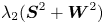
Finally, the  $\lambda _{2}$-criterion of Jeong & Hussain (Reference Jeong and Hussain1995) asserts that a vortex is a collection of points at which the pressure has a local minimum in an appropriate two-dimensional plane. Working with the Navier–Stokes equations and ignoring the acceleration and the viscous terms, Jeong & Hussain (Reference Jeong and Hussain1995) obtain that the intermediate eigenvalue
 $\lambda _{2}(\boldsymbol {S}^{2}+\boldsymbol {W}^{2})$ of the symmetric tensor
 $\boldsymbol {S}^{2}+\boldsymbol {W}^{2}$ should be negative inside such a vortex.
While all these local vortex criteria involve plausible physical arguments in their derivations, their connection to vortical trajectory motion can only be established close enough to steady or slowly varying stagnation points (Haller Reference Haller2000). Due to inconsistencies and inaccuracies in their predictions away from such points, the actual criteria are rarely implemented in their original form. Instead, it has become customary to plot heuristically chosen, instantaneous level surfaces of  $Q$,
 $\varDelta ,$
 $\lambda _{ci},$
 $r_{min}$ and
 $\lambda _{2}$, and view these as coherent structures rendered by the criteria (see, e.g., Dubief & Delcayre Reference Dubief and Delcayre2000; McMullan & Page Reference McMullan and Page2012; Jantzen et al. Reference Jantzen, Taira, Granlund and Ol2014; Gao et al. Reference Gao, Ma, Zambonini, Boudet, Ottavy, Lu and Shao2015; Anghan et al. Reference Anghan, Dave, Saincher and Banerjee2019). These level-surface plots undoubtedly offer quick and often spectacular visualizations. Appropriate tweaking of their (rather sensitive) threshold values will yield similarities across different criteria and consistency with prior analyses of the same flows.
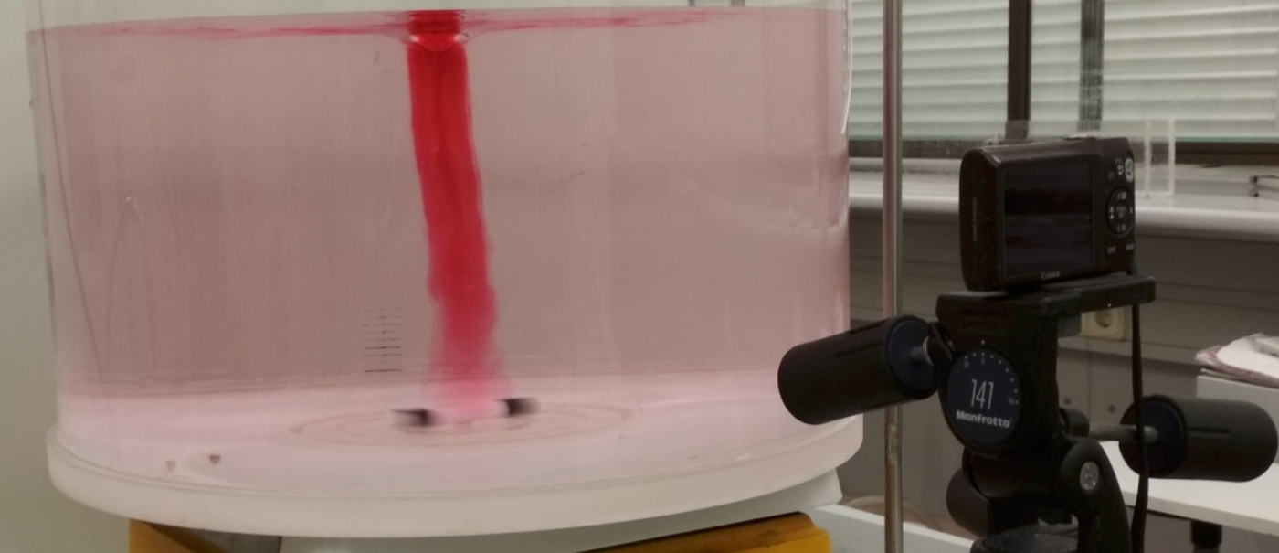
The question, however, remains: do these visually appealing level-surface plots necessarily describe observable flow structures highlighted by passive tracers? The answer to this question turns out to be ‘no’ even for simple, laminar, two-dimensional Navier–Stokes flows (see, e.g., Pedergnana et al. Reference Pedergnana, Oettinger and Haller2020). For more complex flows, a definitive answer is only possible from comparisons with flow visualization experiments, which invariably involve material tracers or weakly diffusive dye, just as the experiment of Tél et al. (Reference Tél, Kadi, Jánosi and Vincze2018) shown in figure 1 does. If one accepts the results of such experiments as the ground truth for coherent vortices, then one accepts that vortices are part of the material deformation field of the fluid.
A coherent material vortex visualized experimentally by dye. Image: courtesy of M. Vincze and T. Tél. See Tél et al. (Reference Tél, Kadi, Jánosi and Vincze2018) for details on the experiment.

Material deformation, however, is frame indifferent (or objective) by one of the main axioms of continuum mechanics Gurtin (Reference Gurtin1981). Indeed, any person or camera moving and turning around in the laboratory shown in figure 1 would visually identify exactly the same physical region as the vortex, even though points in that region would be moving along different trajectories in each observer's frame. Accordingly, any self-consistent criterion for experimentally observable vortices, or more broadly, for experimentally observable coherent structures, should be objective: it should only involve observer-indifferent scalar, vector and tensor fields. This minimal requirement for flow-feature identification was already pointed out in the 1970s by Drouot (Reference Drouot1976), Drouot & Lucius (Reference Drouot and Lucius1976), Astarita (Reference Astarita1979) and Lugt (Reference Lugt1979). More recent reviews by Haller (Reference Haller2005, Reference Haller2015), Peacock, Froyland & Haller (Reference Peacock, Froyland and Haller2015), Kirwan (Reference Kirwan2016) and Günther & Theisel (Reference Günther and Theisel2018) have further elaborated on the need to identify coherent structures in an observer-independent fashion.
Notably, however, none of the local vortex criteria we have surveyed here are objective. Different rotating observers applying these criteria in their own frames will identify different physical regions as vortices using the fluid velocity field of experiment in figure 1 in their own frames. This discrepancy between frame-dependent results from local vortex criteria and frame-indifferent results from experimental observations has prompted several authors to propose objective modifications to these criteria (Martins et al. Reference Martins, Pereira, Mompean, Thais and Thompson2016; Günther, Gross & Theisel Reference Günther, Gross and Theisel2017; Hadwiger et al. Reference Hadwiger, Mlejnek, Theussl and Rautek2018; Liu, Gao & Liu Reference Liu, Gao and Liu2019a; Liu et al. Reference Liu, Gao, Wang and Liu2019b; Günther & Theisel Reference Günther and Theisel2020; Rojo & Günther Reference Rojo and Günther2020). Some of these objectivization procedures involve the formal replacement of the spin tensor with other tensors in the original criteria. Others involve passages to pointwise different local observer frames in the fluid domain.
The latter approach amounts to prescribing a generalized (possibly nonlinear) frame change by specifying its Jacobian at each point in the flow. Approximate numerical implementations of these envisioned coordinate changes will always produce a visual output, because level surfaces of  $Q$,
 $\varDelta ,$
 $\lambda _{ci},$
 $r_{min}$ and
 $\lambda _{2}$ can always be plotted in approximately computed new coordinates. This does not imply, however, that the coordinate changes with the originally envisioned properties actually exist in the absence of those approximations. Even if they do exist, their objectivity is not a priori guaranteed and also requires more detailed arguments than what is typically given in the literature.
In order to identify generally applicable objectivization procedures, we derive here necessary and sufficient conditions for the existence of generalized observer changes defined through their Jacobian fields. We then use these results to scrutinize the existence and objectivity of available objectivization principles, all of which are defined locally through their Jacobians. We find that only the objectivization procedure that replaces the spin tensor  $\boldsymbol {W}$ by its deviation from its spatial mean (Liu et al. Reference Liu, Gao and Liu2019a,Reference Liu, Gao, Wang and Liub) is applicable to generic fluid flows.
2. Objectivization of vortex criteria
A tensor field  $\boldsymbol {A}(\boldsymbol {x},t)$ is objective (Gurtin Reference Gurtin1981; Gurtin, Fried & Anand Reference Gurtin, Fried and Anand2010) if for any time-dependent rotation tensors
 $\boldsymbol {Q}(t)$ and translation vectors
 $\boldsymbol {b}(t)$, the Euclidean frame change
 \begin{equation} \boldsymbol{x}=\boldsymbol{Q}(t)\boldsymbol{y}+\boldsymbol{b}(t) \end{equation}
causes the tensor to transform to the  $\boldsymbol {y}$-frame as
 \begin{equation} \boldsymbol{\tilde{A}}(\boldsymbol{y},t)=\boldsymbol{Q}^{\textrm{T}}(t)\boldsymbol{A}(\boldsymbol{x},t)\boldsymbol{Q}(t). \end{equation}
This is the classic transformation rule in linear algebra that any tensor follows under a time-independent change of the frame of reference. In contrast, a time-dependent frame change may affect the way in which the tensor field  $\boldsymbol {A}(\boldsymbol {x},t)$ is computed in the new frame, invalidating the relationship (2.2). For instance, when recomputed from the velocity field in the new frame, the rate-of-strain tensor
 $\boldsymbol {S}$ turns out to obey the transformation rule (2.2). In contrast, the recomputed spin tensor
 $\boldsymbol {W}$ in the
 $\boldsymbol {y}$-frame takes the form
 \begin{equation} \tilde{\boldsymbol{W}}=\boldsymbol{Q}^{\textrm{T}}\boldsymbol{W}\boldsymbol{Q}-\boldsymbol{Q}^{\textrm{T}}\dot{\boldsymbol{Q}}, \end{equation}
and hence is not objective. This, in turn, renders all local vortex criteria we have surveyed in the Introduction non-objective, given that  $Q$,
 $\varDelta ,$
 $\lambda _{ci},$
 $r_{min}$ and
 $\lambda _{2}$ all depend on
 $\boldsymbol {W}$ explicitly. The level surfaces of these fields, therefore, do not mark experimentally verifiable (material) flow structures. Rather, they mark different physical regions in different observer frames rotating relative to each other. There will be no a priori indication as to which (if any) of these infinitely many different predictions for vortices is correct.
One possible objectivization of local vortex criteria involves the replacement of  $\boldsymbol {W}$ in
 $Q$,
 $\varDelta ,$
 $\lambda _{ci},$
 $r_{min}$ and
 $\lambda _{2}$ with some objective rotation-rate tensor
 $\boldsymbol {W}_{0}$ (Martins et al. Reference Martins, Pereira, Mompean, Thais and Thompson2016; Liu et al. Reference Liu, Gao and Liu2019a,Reference Liu, Gao, Wang and Liub). While this modification makes the criteria formally objective, it also invalidates the original physical arguments used in their derivations. Indeed, in the case of
 $Q,\varDelta ,\lambda _{ci}$ and
 $r_{min}$ fields, the relationship of the local vortex criteria to the equation of variations (1.1) is lost after such a replacement. As for the
 $\lambda _{2}$-field, its relationship to the Navier–Stokes equation is lost after such a replacement, given that
 $\boldsymbol {\nabla }\boldsymbol {v}$ is not equal to
 $\boldsymbol {S}+\boldsymbol {W}_{0}$ in the equation for the pressure Hessian.
An alternative objectivization to vortex criteria is the construction of time-dependent, pointwise Euclidean frame changes prior to the application of these criteria (Tabor & Klapper Reference Tabor and Klapper1994; Lapeyre, Klein & Hua Reference Lapeyre, Klein and Hua1999; Günther et al. Reference Günther, Gross and Theisel2017; Hadwiger et al. Reference Hadwiger, Mlejnek, Theussl and Rautek2018; Liu et al. Reference Liu, Gao and Liu2019a,Reference Liu, Gao, Wang and Liub; Günther & Theisel Reference Günther and Theisel2020; Rojo & Günther Reference Rojo and Günther2020). If the new local frame is defined in an observer-independent fashion (such as, e.g. the frame of the eigenvectors of  $\boldsymbol {S}$), then the evaluation of
 $Q$,
 $\varDelta$,
 $\lambda _{ci}$,
 $r_{min}$ and
 $\lambda _{2}$ in this unique new frame produces objective scalar fields. These locally optimal Euclidean frame changes, however, typically vary from one spatial location to the next, and hence amount to a nonlinear frame change over any open subset of the flow domain. As different physical points will be pronounced to be inside or outside a vortex by different local observers at different times, a straightforward experimental verifiability of predictions from such an objectivization is no longer guaranteed. Proponents of nonlinear frame changes argue that this is not necessarily a negative, because locally optimized observer changes of the form (2.1) may, in fact, enable the discovery of intrinsically connected, global flow features that are only visible locally to any classic observer.
This view, as pointed out by Rojo & Günther (Reference Rojo and Günther2020), is partly motivated by observations of Lugt (Reference Lugt1979) and Perry & Chong (Reference Perry and Chong1994). Indeed, Perry & Chong (Reference Perry and Chong1994) write: ‘ [ $\ldots$] there are patterns, e.g. jets in cross-flow [
 $\cdots$] where there is no single Galilean frame which can be chosen to see all the eddies at once. Here the eddies are accelerating and for a given frame of reference only local parts of the pattern become steady and eddies appear as foci and then only for a short time’. This flow description suggests that one can only reliably identify a region as a vortex if one finds an inertial frame in which that region is steady and has vortical streamlines. In other words, Perry & Chong (Reference Perry and Chong1994) suggest that the streamline geometry of a steady flow is the only acceptable ground truth for vortex identification.
In contrast, contemporary coherent-structure detection methods view vortices as material regions of maximal coherence, which can be objectively established in any (global) Euclidean observer's frame (see, e.g., Haller Reference Haller2005; Froyland, Santitissadeekorn & Monahan Reference Froyland, Santitissadeekorn and Monahan2010; Haller Reference Haller2015; Allshouse & Peacock Reference Allshouse and Peacock2015; Serra & Haller Reference Serra and Haller2016; Epps Reference Epps2017; Haller et al. Reference Haller, Katsanoulis, Holzner, Frohnapfel and Gatti2020). Such methods guarantee simultaneous experimental observability for all identified vortices.
While we fundamentally subscribe to the latter view, we also wish to explore the self-consistency of the former view that promotes spatially inhomogeneous families of local reference frames. This inhomogeneity guarantees no classic experimental observability for the structures identified simultaneously at different locations by different local observers. Yet, as a self-consistency requirement, proponents of this view should insist that all local observers defined at different locations and different times should be compatible with each other. In particular, all local observers must ultimately come to the same conclusion if they approach each other from any direction in space and time. In addition, the locally optimal frames involved in this objectivization procedure should indeed be objectively defined, which has to be verified separately in addition to the compatibility of the local observers.
Next, we will derive sufficient and necessary compatibility conditions that ensure these minimal self-consistency properties for local observers. The conditions we obtain will enable us to verify the feasibility of the generalized, objectivizing frame changes we have cited above. The same compatibility conditions will also allow us to assess whether the formal substitution of  $\boldsymbol {W}$ by some objective tensor field
 $\boldsymbol {W}_{0}$ in local vortex criteria can be justified as a generalized frame change.
3. Compatibility conditions for generalized frame changes
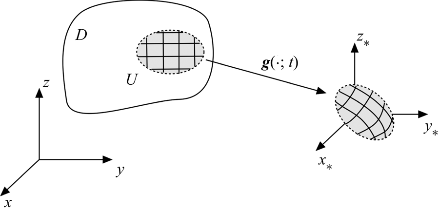
A generalized frame change is a time-dependent change of variables
 \begin{equation} \boldsymbol{x}_{*}=\boldsymbol{g}(\boldsymbol{x};t),\qquad\boldsymbol{x}\in U,\quad \boldsymbol{x}_{*}\in\mathbb{R}^{3}, \end{equation}
where the local diffeomorphism  $\boldsymbol {g}(\cdot;t)\colon U\to \mathbb {R}^{3}$ is defined over an open subset
 $U$ of the flow domain
 $D$, as shown in figure 2. Without loss of generality, we will choose
 $U$ to be simply connected. The observer change (3.1) depends on the time
 $t\in [t_{0},t_{1}]$, where
 $[t_{0},t_{1}]$ is the interval over which the velocity field
 $\boldsymbol {v}$ is available.
A nonlinear frame change  $\boldsymbol {g}(\cdot;t)\colon (x,y,z) \mapsto (x_*,y_*,z_*)\in \mathbb {R}^{3}$, defined locally on a simply connected open set
 $U$ within the flow domain
 $D\subset \mathbb {R}^{3}$ for times
 $t\in [t_0,t_1]$.

Frame changes falling in the general class (3.1) have been proposed either implicitly or explicitly by Astarita (Reference Astarita1979), Tabor & Klapper (Reference Tabor and Klapper1994), Lapeyre et al. (Reference Lapeyre, Klein and Hua1999), Günther et al. (Reference Günther, Gross and Theisel2017), Hadwiger et al. (Reference Hadwiger, Mlejnek, Theussl and Rautek2018), Liu et al. (Reference Liu, Gao and Liu2019a,Reference Liu, Gao, Wang and Liub), Günther & Theisel (Reference Günther and Theisel2020) and Rojo & Günther (Reference Rojo and Günther2020). In these references, the transformation  $\boldsymbol {g}$ is constructed pointwise in
 $U$ from local, linear observer changes prescribed as
 \begin{equation} {\textrm{d}\boldsymbol{x}}_{*}=\partial_{\boldsymbol{x}}\boldsymbol{g}(\boldsymbol{x};t)\,{\textrm{d}\boldsymbol{x}}=\boldsymbol{G}(\boldsymbol{x};t)\,\textrm{d}\boldsymbol{x}. \end{equation}
For instance, the prescribed Jacobian field  $\boldsymbol {G}(\boldsymbol {x};t)$ field may be a time-dependent rotation tensor field that makes
 $\boldsymbol {v}$ locally as steady as possible (Günther et al. Reference Günther, Gross and Theisel2017; Hadwiger et al. Reference Hadwiger, Mlejnek, Theussl and Rautek2018; Günther & Theisel Reference Günther and Theisel2020; Rojo & Günther Reference Rojo and Günther2020). As another example,
 $\boldsymbol {G}(\boldsymbol {x};t)$ may align the coordinate axes locally with the eigenvectors of
 $\boldsymbol {S}(\boldsymbol {x},t)$ (Astarita Reference Astarita1979; Tabor & Klapper Reference Tabor and Klapper1994; Lapeyre et al. Reference Lapeyre, Klein and Hua1999).
Differentiation of (3.1) with respect to time along trajectories gives the transformed velocity field
 \begin{equation} \boldsymbol{v}_{*}(\boldsymbol{x}_{*},t)=\partial_{\boldsymbol{x}}\boldsymbol{g}(\boldsymbol{g}^{-1}(\boldsymbol{x}_{*};t);t)\boldsymbol{v}(\boldsymbol{g}^{-1}(\boldsymbol{x}_{*};t),t)+\partial_{t}\boldsymbol{g}(\boldsymbol{g}^{-1}(\boldsymbol{x}_{*};t);t). \end{equation}
All objectivized vortex criteria we have cited involve the evaluation of the original vortex criteria on the velocity field (3.3). This evaluation requires the computation of the transformed velocity gradient  $\boldsymbol {\nabla _{*}}\boldsymbol {v}_{*}$ and its strain-spin decomposition, which are given by the formulae
 \begin{gather} \boldsymbol{\nabla_{*}}\boldsymbol{v}_{*} =\boldsymbol{G}\boldsymbol{\nabla}\boldsymbol{v}\boldsymbol{G}^{-1} +\partial_{t}\boldsymbol{G}\boldsymbol{G}^{-1}+\boldsymbol{\nabla}\boldsymbol{G} \boldsymbol{G}^{-1}\boldsymbol{v}, \end{gather}
 \begin{gather} \boldsymbol{S}_{*}=\tfrac{1}{2}[\boldsymbol{\nabla_{*}}\boldsymbol{v}_{*}+ [\boldsymbol{\nabla_{*}}\boldsymbol{v}_{*}]^{\textrm{T}}],\quad\boldsymbol{W}_{*}=\tfrac{1}{2}[\boldsymbol{\nabla_{*}}\boldsymbol{v}_{*}-[\boldsymbol{\nabla_{*}}\boldsymbol{v}_{*}]^{\textrm{T}}]. \end{gather}
Note that any temporally smooth,  $\boldsymbol {x}$-independent choice of
 $\boldsymbol {G}(t)$ in (3.2) yields the global Euclidean frame change
 $\boldsymbol {x}_*=\boldsymbol {G}(t)\boldsymbol {x}+\boldsymbol {c}(t)$, which is well defined up to a constant translation vector
 $\boldsymbol {c}(t)$. Such frame changes have been used, e.g. by Tabor & Klapper (Reference Tabor and Klapper1994), Lapeyre et al. (Reference Lapeyre, Klein and Hua1999) and Haller (Reference Haller2001) to analyse the equation of variations (1.1) along a single fluid trajectory
 $\boldsymbol {x}(t)$. These studies select
 $\boldsymbol {G}(t)$ to provide an advantageous set of coordinates
 \begin{equation} \boldsymbol{x}_{*}=\boldsymbol{g}(\boldsymbol{x};t)=\boldsymbol{G}(t)\left[\boldsymbol{x}-\boldsymbol{x}(t)\right] \end{equation}
for the analysis of the stability of  $\boldsymbol {x}(t)$. The velocity field in this new, globally defined frame is then
 $\boldsymbol {\nabla _{*}}\boldsymbol {v}_{*}=\boldsymbol {G}\,\boldsymbol {\nabla }\boldsymbol {v}\,\boldsymbol {G}^{-1}+\partial _{t}\boldsymbol {G}\,\boldsymbol {G}^{-1},$ lacking the third term in (3.4).
In contrast, proposed objectivizations of coherent-structure visualizations involve level-surface plots of scalar fields obtained after changing coordinates simultaneously at each point of the flow domain, as in (3.2). Then, calculating the velocity gradient  $\boldsymbol {\nabla _{*}}\boldsymbol {v}_{*}$ at any point, one must not forget that similar frame changes have been carried out at all neighbouring points in the flow as well. This spatial dependence is responsible for the third term in the general expression for
 $\boldsymbol {\nabla _{*}}\boldsymbol {v}_{*}$ in (3.4). Omitting this term implies that one compares information from different points of infinitely many different velocity fields, each obtained from a different global frame change of the form (3.6) with a different choice of
 $\boldsymbol {x}(t)$. Clearly, for coherent-structure analysis in a given flow, one should compare information from different points of the same velocity field at time
 $t$. As we will see in the next section, the third term in (3.4) has nevertheless been consistently forgotten or ignored in proposed objectivization procedures.
To ensure that the quantities (3.3)–(3.5a,b) are indeed computable and give self-consistent results, we need to require the following minimal compatibility conditions to hold.
Definition 3.1 The local observer changes defined in (3.2) are compatible if the following two conditions hold:
(i) All local observers are able to evaluate local vortex criteria in their frames.
(ii) All local observes reach asymptotically the same conclusion from these criteria as the observer locations and the observation times approach each other.
Our main result is a necessary and sufficient condition that ensures the compatibility of local observer changes in the sense of definition 3.1. To state this criterion, we will use the notation  $C^{1}(U\times \mathbb {R})$ for the class of continuously differentiable tensor fields with arguments
 $(\boldsymbol {x},t)\in U\times \mathbb {R}$. Furthermore, we will use
 $\boldsymbol {\nabla }\times \boldsymbol {G}$ to denote the tensor whose rows are the curls of the rows of
 $\boldsymbol {G}$.
Theorem 3.2 The local observer changes (3.2) are compatible if and only if
 \begin{gather} \boldsymbol{G},\boldsymbol{G}^{-1} \in C^{1}\left(U\times\mathbb{R}\right), \end{gather}
 \begin{gather}\boldsymbol{\nabla}\times\boldsymbol{G} =\boldsymbol{0}. \end{gather}
Proof. For the compatibility requirement (i) in definition 3.1 to hold, the velocity field (3.3) must be well defined and at least once continuously differentiable in its arguments, which requires (3.7) to be satisfied. We also need to ensure, however, that the transformation  $\boldsymbol {g}$ is well defined (up a to a constant) on a small enough open neighbourhood
 $U$ near each point
 $\boldsymbol {x}$ in the flow domain. This needs to be guaranteed separately, because only the Jacobian field
 $\boldsymbol {G}(\boldsymbol {x},t)$ of
 $\boldsymbol {g}(\boldsymbol {x},t)$, as opposed to
 $\boldsymbol {g}(\boldsymbol {x},t)$ itself, is specified in the local observer changes (3.2). Without a well-defined local diffeomorphism
 $\boldsymbol {g}(\boldsymbol {x},t)$ on
 $U$, formula (3.4) would not be valid, as
 $\boldsymbol {g}^{-1}(\boldsymbol {x}_{*};t)$ would not be well defined and differentiable.
To ensure that the  $\boldsymbol {g}$ field is well defined at least on a small enough open set
 $U$, we first note that in the original Euclidean
 $\boldsymbol {x}$-coordinates, the local relation (3.2) implies
 \begin{equation} \boldsymbol{G}=\begin{bmatrix} G_{11} & G_{12} & G_{13}\\ G_{21} & G_{22} & G_{23}\\ G_{31} & G_{32} & G_{33} \end{bmatrix}=\begin{bmatrix} \partial_{\boldsymbol{x}}g_{1}\\ \partial_{\boldsymbol{x}}g_{2}\\ \partial_{\boldsymbol{x}}g_{3} \end{bmatrix}, \end{equation}
where  $\boldsymbol {g}=(g_{1},g_{2},g_{3})$. This means that for any time
 $t$, the
 $i$th row of
 $\boldsymbol {G}$ must be a gradient vector field associated with the scalar potential function
 $g_{i}(\boldsymbol {x},t)$ in the original
 $\boldsymbol {x}$-frame. By classic multivariable calculus applied on the simply connected domain
 $U$, the vector field
 $(G_{i1},G_{i2},G_{i3})$ admits a potential if and only if it is curl free, i.e.
 $\boldsymbol {\nabla }\times (G_{i1},G_{i2},G_{i3})\equiv \boldsymbol {0}$ for
 $i=1,2,3$. Therefore, defining
 $\boldsymbol {\nabla }\times \boldsymbol {G}$ as a tensor whose rows are the curls of the rows of
 $\boldsymbol {G}$, we obtain the second observer compatibility condition (3.8).
We have not required the local observer changes defined in (3.2) to be necessarily Euclidean (distance preserving). Therefore, theorem 3.2 is also applicable to the non-Euclidean local observer changes considered in Hadwiger et al. (Reference Hadwiger, Mlejnek, Theussl and Rautek2018) and Günther & Theisel (Reference Günther and Theisel2020). We note, however, that all local vortex criteria surveyed in the Introduction assume that the flow is incompressible. Therefore, these criteria can only be applied to the transformed velocity field  $\boldsymbol {v}_{*}$ directly if
 $\boldsymbol {g}$ is volume preserving, i.e.
 $\det \boldsymbol {G}\equiv 1$.
4. Evaluation of available objectivization procedures
Here we examine whether the objectivization procedures available in the literature satisfy the compatibility conditions we have obtained in theorem 3.2.
4.1. Replacing  ${W}$ with the relative spin tensor

With the help of an orthonormal basis  $\{ \boldsymbol {e}_{i}(\boldsymbol {x},t)\} _{i=1}^{3}$ of the rate-of-strain tensor
 $\boldsymbol {S}(\boldsymbol {x},t)$, we can define the strain-rotation-rate tensor
 \begin{equation} \boldsymbol{W}_{s}\left(\boldsymbol{x},t\right):=-\sum_{i=1}^{3}\boldsymbol{e}_{i}\left(\boldsymbol{x},t\right)\left[\frac{\textrm{D}}{\textrm{D}t}\boldsymbol{e}_{i}\left(\boldsymbol{x},t\right)\right]^{\textrm{T}}. \end{equation}
Then, as observed by Drouot (Reference Drouot1976), Drouot & Lucius (Reference Drouot and Lucius1976), Astarita (Reference Astarita1979) and others, the relative spin tensor,
 \begin{equation} \boldsymbol{W}_{r}=\boldsymbol{W}-\boldsymbol{W}_{s}, \end{equation}
is objective. Motivated by this observation or by other considerations, various authors have suggested modifying local vortex criteria by replacing  $\boldsymbol {W}$ pointwise with
 $\boldsymbol {W}_{r}$ in these criteria (Tabor & Klapper Reference Tabor and Klapper1994; Lapeyre et al. Reference Lapeyre, Klein and Hua1999; Martins et al. Reference Martins, Pereira, Mompean, Thais and Thompson2016). As we have already noted in the Introduction, such a formal replacement removes the (mathematically heuristic but physically at least plausible) relationship between these vortex criteria and the equation of variations (1.1) used in their derivations. This objectivization approach is, therefore, only justifiable, if it can be shown to be equivalent to a generalized frame change (3.1) that transforms the original velocity gradient
 $\boldsymbol {\nabla }\boldsymbol {v}=\boldsymbol {S}+\boldsymbol {W}$ to
 $\boldsymbol {\nabla }\boldsymbol {v}_{r}=\boldsymbol {S}+\boldsymbol {W}_{r}$.
Astarita (Reference Astarita1979) argues that this is in fact the case. He fixes a spatial location  $\boldsymbol {x}_{0}$ and introduces a global Euclidean observer change of the form (2.1), defined with
 $\boldsymbol {b}(t)\equiv \boldsymbol {0}$ and with
 \begin{equation} \boldsymbol{G}^{\textrm{T}}(t):=\left[\boldsymbol{e}_{1}(\boldsymbol{x}_{0},t)\,\boldsymbol{e}_{2}(\boldsymbol{x}_{0},t)\,\boldsymbol{e}_{3}(\boldsymbol{x}_{0},t)\right], \end{equation}
where  $\boldsymbol {e}_{i}(\boldsymbol {x}_{0},t)$ forms the
 $i$th column of
 $\boldsymbol {G}^{\textrm {T}}(t)$. Observing that
 $({\textrm {D}}/{\textrm {D}t})\boldsymbol {e}_{i}=\boldsymbol {W}_{s}\boldsymbol {e}_{i}$ from the definition of
 $\boldsymbol {W}_{s}$ in (4.1), one obtains a matrix differential equation for
 $\boldsymbol {\boldsymbol {G}}(t)$ in the form
 \begin{equation} \dot{\boldsymbol{\boldsymbol{G}}}^{\textrm{T}}(t)=\boldsymbol{W}_{s}(\boldsymbol{x}_{0},t)\boldsymbol{\boldsymbol{G}}^{\textrm{T}}(t). \end{equation}
Then, using the transformation formula (3.4) together with (4.4), Astarita (Reference Astarita1979) obtains
 \begin{align} \left.\boldsymbol{\nabla}_{*}\boldsymbol{v}_{*}\right|_{\boldsymbol{x}=\boldsymbol{x}_{0}} &=\left.\boldsymbol{G}\left[\boldsymbol{S}+\boldsymbol{W}\right]\boldsymbol{G}^{\textrm{T}}+\dot{\boldsymbol{G}}\boldsymbol{\boldsymbol{G}}^{\textrm{T}}\right|_{\boldsymbol{x}=\boldsymbol{x}_{0}}\nonumber\\ &=\left.\boldsymbol{G}\left[\boldsymbol{S}+\boldsymbol{W}\right]\boldsymbol{G}^{\textrm{T}}-\boldsymbol{G}\boldsymbol{W}_{s}\boldsymbol{\boldsymbol{G}}^{\textrm{T}}\right|_{\boldsymbol{x}=\boldsymbol{x}_{0}}\nonumber\\ &=\left.\boldsymbol{G}\boldsymbol{\nabla}\boldsymbol{v}_{r}\boldsymbol{\boldsymbol{G}}^{\textrm{T}}\right|_{\boldsymbol{x}=\boldsymbol{x}_{0}} . \end{align}
This proves that the gradient  $\boldsymbol {\nabla }\boldsymbol {v}_{r}(\boldsymbol {x}_{0},t)$ becomes
 $\boldsymbol {\nabla }_{*}\boldsymbol {v}_{*}(\boldsymbol {x}_{0},t)$. By the objectivity of
 $\boldsymbol {\nabla }\boldsymbol {v}_{r}$, therefore, evaluating local vortex criteria on
 $\boldsymbol {\nabla }\boldsymbol {v}_{r}(\boldsymbol {x}_{0},t)$ will give the same result as evaluating these criteria on
 $\boldsymbol {\nabla }\boldsymbol {v}$ after the Euclidean frame change defined by
 $\boldsymbol {G}(t)$ in (4.3).
The problem with this argument is that it ignores the spatial dependence of the basis  $\{ \boldsymbol {e}_{i}(\boldsymbol {x},t)\} _{i=1}^{3}$ and hence the dependence of
 $\boldsymbol {G}(t)$ on
 $\boldsymbol {x}$ in this construct. The global Euclidean frame change (4.3) indeed transforms
 $\boldsymbol {\nabla }\boldsymbol {v}(\boldsymbol {x}_{0},t)$ to strain basis at the point
 $\boldsymbol {x}_{0}$ but not at a general point
 $\boldsymbol {x}$. Once one accounts for the spatial dependence of
 $\boldsymbol {G}$, the proposed change to strain eigenbasis becomes a nonlinear frame change
 $\boldsymbol {g}(\boldsymbol {x};t)$ whose existence on open neighbourhoods of the flow domain needs to be verified via theorem 3.2 (see the related discussion before definition 3.1). All this was also overlooked by Haller (Reference Haller2001, Reference Haller2005) in his assessment of the objectivization procedure based on
 $\boldsymbol {W}_{r}$.
The correct local form of the generalized frame change to the strain eigenbasis  $\{ \boldsymbol {e}_{i}(\boldsymbol {x},t)\} _{i=1}^{3}$ is defined by (3.2) with
 \begin{equation} \boldsymbol{G}^{\textrm{T}}(\boldsymbol{x},t)=\left[\boldsymbol{e}_{1}(\boldsymbol{x},t)\,\boldsymbol{e}_{2}(\boldsymbol{x},t)\,\boldsymbol{e}_{3}(\boldsymbol{x},t)\right]. \end{equation}
By the symmetry of  $\boldsymbol {S}$, its orthonormal eigenbasis is a continuously differentiable function of
 $(\boldsymbol {x},t)$ as long as
 $\boldsymbol {v}$ is twice continuously differentiable. Therefore, the first compatibility condition in (3.7) is satisfied. The second compatibility condition (3.8), however, generically fails
 \begin{equation} \boldsymbol{\nabla}\times\left[\boldsymbol{e}_{1}(\boldsymbol{x},t)\,\boldsymbol{e}_{2}(\boldsymbol{x},t)\,\boldsymbol{e}_{3}(\boldsymbol{x},t)\right]^{\textrm{T}}\neq\boldsymbol{0}. \end{equation}
This is because the eigenvector fields  $\boldsymbol {e}_{i}(\boldsymbol {x},t)$ are generically not conservative vector fields and hence their curl does not vanish. We conclude that the pointwise replacement of
 $\boldsymbol {\nabla }\boldsymbol {v}$ by
 $\boldsymbol {\nabla }\boldsymbol {v}_{r}$ in local vortex criteria cannot generally be viewed as a result of a nonlinear observer change.
To illustrate this, we consider the simple steady, incompressible velocity field
 \begin{equation} \boldsymbol{v}(\boldsymbol{x})=(y+x^{2}-y^{2},-x-2xy,0), \end{equation}
a member of the general class of universal (i.e. viscosity-independent) Navier–Stokes velocity fields identified by Pedergnana et al. (Reference Pedergnana, Oettinger and Haller2020). For this flow, we obtain that the matrix of orthonormal rate-of-strain eigenvectors, as defined in (4.6), is of the form
 \begin{gather} \boldsymbol{G}(\boldsymbol{x},t)=\begin{pmatrix} 0 & 0 & 1\\ -\dfrac{x-\sqrt{x^{2}+y^{2}}}{\sqrt{2}\sqrt{x^{2}-x\sqrt{x^{2}+y^{2}}+y^{2}}} & \dfrac{y}{\sqrt{2}\sqrt{x^{2}-x\sqrt{x^{2}+y^{2}}+y^{2}}} & 0\\ -\dfrac{x+\sqrt{x^{2}+y^{2}}}{\sqrt{2}\sqrt{x^{2}+x\sqrt{x^{2}+y^{2}}+y^{2}}} & \dfrac{y}{\sqrt{2}\sqrt{x^{2}+x\sqrt{x^{2}+y^{2}}+y^{2}}} & 0 \end{pmatrix}. \end{gather}
This is a continuously differentiable rotation tensor field with a continuously differentiable inverse (transpose) on all simply connected, open neighbourhoods  $U$ that do not intersect the plane
 $\{ \boldsymbol {x}\in \mathbb {R}^{3}:y=0\}$. Therefore, the first compatibility condition (3.7) holds on all such neighbourhoods. The curl of the tensor field
 $\boldsymbol {G}$, on any such
 $U$ neighbourhood is strictly non-zero, given by
 \begin{equation} \boldsymbol{\nabla}\times\boldsymbol{G}(\boldsymbol{x},t)=\begin{pmatrix} 0 & 0 & 0\\ 0 & 0 & \dfrac{\sqrt{2}y\left(3x^{2}-3x\sqrt{x^{2}+y^{2}}+y^{2}\right)}{4\sqrt{x^{2}+y^{2}}\left(x^{2}-x\sqrt{x^{2}+y^{2}}+y^{2}\right)^{3/2}}\\ 0 & 0 & -\dfrac{\sqrt{2}y\left(3x^{2}+3x\sqrt{x^{2}+y^{2}}+y^{2}\right)}{4\sqrt{x^{2}+y^{2}}\left(x^{2}+x\sqrt{x^{2}+y^{2}}+y^{2}\right)^{3/2}}\end{pmatrix}\neq\boldsymbol{0}.\end{equation}
Therefore, the second compatibility condition (3.8) of theorem 3.2 is violated. Consequently, no compatible generalized frame change to the rate-of-strain eigenbasis exists for the steady velocity field (4.8) on any open subset of  $U$ with
 $U\cap \{y=0\}=\emptyset$ for the velocity field (4.8).
4.2. Replacing ${v}$ with its minimally unsteady component

To objectivize all local vortex criteria for a smooth velocity field  $\boldsymbol {v}(\boldsymbol {x},t)$, Günther et al. (Reference Günther, Gross and Theisel2017) propose applying them after a generalized frame change
 $\boldsymbol {g}(\boldsymbol {x},t)$ that pointwise minimizes the unsteadiness of
 $\boldsymbol {v}$. As formulated more generally in follow-up work by Rojo & Günther (Reference Rojo and Günther2020), the proposed unsteadiness measure to be minimized over all choices of
 $\boldsymbol {g}$ is
 \begin{equation} J_{t}(\boldsymbol{g})=\int_{U}\left|\partial_{t}\boldsymbol{v}_{*}(\boldsymbol{x}_{\boldsymbol{*}},t)\right|^{2}\,\textrm{d}V, \end{equation}
with  $\boldsymbol {v}_{*}$ computed from
 $\boldsymbol {v}$ using the frame change
 $\boldsymbol {g}$, based on formula (3.3).
To evaluate  $\partial _{t}\boldsymbol {v}_{*}(\boldsymbol {x}_{\boldsymbol {*}},t)$ in this expression and apply local vortex criteria to the minimally unsteady
 $\hat {\boldsymbol {v}}_{*}$ arising from the minimization procedure, one needs to consider twice continuously differentiable generalized observer changes
 $\boldsymbol {g}$ (see formula (3.3)) in minimizing
 $J_{t}(\boldsymbol {g})$. Therefore, the unsteadiness-minimizing transformation
 $\hat {\boldsymbol {g}}$ for the velocity field
 $\boldsymbol {v}$ at time
 $t$ can technically be sought as
 \begin{equation} \hat{\boldsymbol{g}}=\mathop{\text{arg min}}\limits_{\boldsymbol{g}\in C^{2}\left(U\times[t-\epsilon,t+\epsilon]\right)}J_{t}(\boldsymbol{g}), \end{equation}
for some small non-zero parameter  $\epsilon >0$. Under further assumptions and boundary conditions, this calculus of variations problem may have a unique solution for
 $\boldsymbol {g}$ which would then automatically satisfy the compatibility conditions of our theorem 3.2. As we show in appendix A, however, unsteadiness-minimizing transforms of
 $\boldsymbol {v}$ (under any self-consistent measure of unsteadiness, including
 $J_{t}$ in (4.12)) are never objective. Therefore, contrary to the assertions of Günther et al. (Reference Günther, Gross and Theisel2017), as well as those of Hadwiger et al. (Reference Hadwiger, Mlejnek, Theussl and Rautek2018), Günther & Theisel (Reference Günther and Theisel2020) and Rojo & Günther (Reference Rojo and Günther2020), applications of local vortex criteria to minimally unsteady transforms of
 $\boldsymbol {v}$ do not constitute objectivizations of those criteria.
In addition to the fundamental non-objectivity of unsteadiness-minimizing frame changes, further issues arise with the proposed numerical implementations of the original optimization problem (4.12). Specifically, Günther et al. (Reference Günther, Gross and Theisel2017) relax the calculus of variations problem (4.12) by adding the constraint
 \begin{equation} \hat{\boldsymbol{G}}(\boldsymbol{x},t)\equiv\boldsymbol{I} \end{equation}
at each point  $\boldsymbol {x}$ and each time instant
 $t$. They then proceed to minimize
 $J_{t}(\boldsymbol {g})$ via the choice of the derivatives
 $\partial _{t}\boldsymbol {G}(\boldsymbol {x},t)$ and
 $\partial _{t}^{2}\hat {\boldsymbol {G}}(\boldsymbol {x},t)$ that arise in the expression for
 $\partial _t\boldsymbol {v}_{*}$.
The choice of  $\hat {\boldsymbol {G}}$ in (4.13) satisfies both compatibility conditions in Theorem 3.2 and hence indeed defines a unique (up to a constant) generalized observer change
 $\hat {\boldsymbol {g}}(\boldsymbol {x},t)$ to this relaxed optimization problem. That solution, however, is simply
 \begin{equation} \hat{\boldsymbol{g}}(\boldsymbol{x},t)=\boldsymbol{x}+\boldsymbol{c}(t). \end{equation}
This coordinate shift does not allow for the optimization envisioned by Günther et al. (Reference Günther, Gross and Theisel2017) over choices of  $\partial _{t}\boldsymbol {G}(\boldsymbol {x},t)$ and
 $\partial _{t}^{2}\hat {\boldsymbol {G}}(\boldsymbol {x},t)$, given that
 \begin{equation} \partial_{t}\hat{\boldsymbol{G}}=\partial_{t}\boldsymbol{\nabla}\hat{\boldsymbol{g}}(\boldsymbol{x},t)\equiv\boldsymbol{0},\qquad\partial_{t}^{2}\hat{\boldsymbol{G}}=\partial_{t}^{2}\boldsymbol{\nabla}\hat{\boldsymbol{g}}(\boldsymbol{x},t)\equiv\boldsymbol{0} \end{equation}
must hold by (4.14).
Günther et al. (Reference Günther, Gross and Theisel2017) and Günther & Theisel (Reference Günther and Theisel2020) address this issue in passing by stating that they assume the local observers changes to be locally constant over an unspecified open neighbourhood of each point in space and time. But an everywhere locally constant smooth function is globally constant and hence its derivatives cannot be chosen freely. Rojo & Günther (Reference Rojo and Günther2020) allow for spatial dependence in the time derivatives of the nonlinear observer change, but still restrict the observer change itself to be the identity map globally. These self-contradicting assumptions are designed to make the underlying optimization problem formally solvable, but the solutions obtained in this fashion lack physical meaning. In particular, no local observer will be able to observe the formally computed velocity field and its derivatives over any non-zero length of time.
In their related approach, Hadwiger et al. (Reference Hadwiger, Mlejnek, Theussl and Rautek2018) face similar problems by not accounting for the  $\boldsymbol {x}$-dependence of the initial conditions of the flow of their proposed observer vector field. In addition, these authors use frame-change formulae for rotating observers that do not account for the rotation of the observer.
In summary, unsteadiness-minimizing procedures lead to calculus of variations problems, such as (4.12). These problems can, in principle, have well-posed solutions for the nonlinear frame change  $\boldsymbol {g}$ under further assumptions. Such solutions then automatically satisfy the requirements of our theorem 3.2 by construction, but cannot be objective, as we show in appendix A. Furthermore, despite the spectacular visualizations they provide, available numerical implementations of the optimization problem (4.12) suffer from physical and mathematical inconsistencies.
4.3. Replacing ${W}$ with the spin-deviation tensor

Liu et al. (Reference Liu, Gao and Liu2019a) propose to objectivize the vortex (or rortex) criterion of Tian et al. (Reference Tian, Gao, Dong and Liu2018) by replacing the velocity gradient  $\boldsymbol {\nabla }\boldsymbol {v}=\boldsymbol {S}+\boldsymbol {W}$ in the computation of
 $Q$ and
 $r_{min}$ with the modified velocity gradient tensor
 \begin{equation} \boldsymbol{\nabla}\boldsymbol{v}_{*}:=\boldsymbol{S}+\boldsymbol{W}-\boldsymbol{\bar{W}}, \end{equation}
where the mean-spin tensor  $\boldsymbol {\bar {W}}(t)=({1}/{\mathrm {vol}U})\int _{U}\boldsymbol {W}\,\textrm {d}V$ is computed over a chosen fluid volume
 $U$. (This volume,
 $U$, is typically the full flow domain on which velocity data are available, but one may also choose a smaller domain to establish a reference value for the mean spin of the flow. The tensor
 $\boldsymbol {\bar {W}}$ is, therefore, dependent on the choice of the domain
 $U$.) This procedure is motivated by the observation of Haller (Reference Haller2016) and Haller et al. (Reference Haller, Hadjighasem, Farazmand and Huhn2016) that the spin-deviation tensor
 $\boldsymbol {W}-\boldsymbol {\bar {W}}$ is objective by formula (2.3). This observation implies that under any Euclidean transformation (2.1), the objectivity condition (2.2) holds, rendering
 \begin{equation} \widetilde{\boldsymbol{\nabla}\boldsymbol{v}}_{*}=\boldsymbol{Q}^{\textrm{T}}\boldsymbol{\nabla}\boldsymbol{v}_{*}\boldsymbol{Q}. \end{equation}
Therefore, by the definition (2.2) of objectivity for tensors, the tensor  $\boldsymbol {\nabla }\boldsymbol {v}_{*}$ defined in (4.16) is objective.
As we have already noted, the formal replacement of the velocity gradient with  $\boldsymbol {\nabla }\boldsymbol {v}^{*}$ (or, equivalently, the replacement of
 $\boldsymbol {W}$ by
 $\boldsymbol {W}-\boldsymbol {\bar {W}}$) in the rortex criterion invalidates the original arguments leading to this criterion, unless this replacement is equivalent to a generalized observer change. One may construct such an observer change locally, using the local observer change formula (3.2) and choosing the spatially constant tensor
 $\boldsymbol {G}(t)$ as a fundamental matrix solution of the initial value problem
 \begin{equation} \dot{\boldsymbol{G}}=\boldsymbol{\bar{W}}(t)\boldsymbol{G},\quad\boldsymbol{G}(t_{0})=\boldsymbol{I}. \end{equation}
Here,  $t_{0}$ is an arbitrary initial time at which the velocity field
 $\boldsymbol {v}(\boldsymbol {x},t)$ is known. Then, the general transformation formula (3.4) for the velocity gradient implies
 \begin{equation} \tilde{\boldsymbol{\nabla}}\tilde{\boldsymbol{v}}=\boldsymbol{G}^{\textrm{T}}\boldsymbol{\nabla}\boldsymbol{v}\boldsymbol{G}-\boldsymbol{G}^{\textrm{T}}\dot{\boldsymbol{\boldsymbol{G}}}=\boldsymbol{G}^{\textrm{T}}\boldsymbol{\nabla}\boldsymbol{v}\boldsymbol{G}-\boldsymbol{G}^{\textrm{T}}\boldsymbol{\bar{W}}\boldsymbol{G}=\boldsymbol{G}^{\textrm{T}}\boldsymbol{\nabla}\boldsymbol{v}^{*}\boldsymbol{G} =\widetilde{\boldsymbol{\nabla}\boldsymbol{v}}_{*}, \end{equation}
where we have used (4.17). Therefore, the local observer change (3.2), with the choice of  $\boldsymbol {G}$ as in (4.18a,b), indeed transforms
 $\boldsymbol {\nabla }\boldsymbol {v}$ into
 $\boldsymbol {\nabla }\boldsymbol {v}_{*}$ in the new frame. In other words, we have found a special frame in which the non-objective
 $\boldsymbol {\nabla }\boldsymbol {v}$ happens to coincide with the objective tensor
 $\boldsymbol {\nabla }\boldsymbol {v}_{*}$. If one then applies a further observer change (such as the inverse of (3.2) with
 $\boldsymbol {G}$ as in (4.18a,b)) to this special frame, then the tensor
 $\boldsymbol {\nabla }\boldsymbol {v}$ will not transform according to the rule (2.2), whereas the objective tensor
 $\boldsymbol {\nabla }\boldsymbol {v}_{*}$, as defined in formula (4.16), will.
The skew symmetry of  $\boldsymbol {\bar {W}}(t)$ then implies that
 $\boldsymbol {G}(t)$ is a proper rotation matrix for all times. As a fundamental matrix solution,
 $\boldsymbol {G}(t)$ is also continuously differentiable in time and has a continuously differentiable inverse. Therefore, the first compatibility condition (3.7) of theorem 3.2 is satisfied. The tensor
 $\boldsymbol {G}(t)$ also satisfies the second compatibility condition (3.8) due to its lack of spatial dependence.
We conclude from Theorem 3.2 that a global observer change exists that is equivalent to the replacement of the  $\boldsymbol {\nabla }\boldsymbol {v}$ with
 $\boldsymbol {\nabla }\boldsymbol {v}^{*}$ defined in (4.16) in any local vortex criterion, including the rortex criterion of Liu et al. (Reference Liu, Gao and Liu2019a). Indeed, the global Euclidean observer change
 $\boldsymbol {x}_{*}=\boldsymbol {G}(t)\boldsymbol {x}$ exists and justifies the objectivization principle of Liu et al. (Reference Liu, Gao and Liu2019a,Reference Liu, Gao, Wang and Liub) on the full flow domain. The spatial homogeneity of the frame change defined in (4.18a,b) also enables experimental verifiability for the structures predicted by the objectivized vortex criteria.
For example, for two-dimensional flows, the initial value problem (4.18a,b) takes the form.
 \begin{equation} \dot{\boldsymbol{G}}=\begin{pmatrix} 0 & \tfrac{1}{2}\bar{\omega}(t)\\ -\tfrac{1}{2}\bar{\omega}(t) & 0\end{pmatrix} \boldsymbol{G},\quad\boldsymbol{G}(t_{0})=\boldsymbol{I}, \end{equation}
with  $\bar {\omega }(t)$ denoting the spatial average of the scalar vorticity field
 $\omega (\boldsymbol {x},t)$ over the flow domain
 $U$. The non-autonomous problem (4.20) can be solved in polar coordinates to yield
 \begin{equation} \boldsymbol{G}(t)=\left(\begin{array}{@{}rc@{}} \cos[\tfrac{1}{2}\int_{t_{0}}^{t}\bar{\omega}(s)\,\textrm{d}s] & \sin[\tfrac{1}{2}\int_{t_{0}}^{t}\bar{\omega}(s)\,\textrm{d}s]\\ -\sin[\tfrac{1}{2}\int_{t_{0}}^{t}\bar{\omega}(s)\,\textrm{d}s] & \cos[\tfrac{1}{2}\int_{t_{0}}^{t}\bar{\omega}(s)\,\textrm{d}s] \end{array}\right). \end{equation}
Therefore, in two dimensions, replacing the spin tensor  $\boldsymbol {W}$ in classic vortex criteria with
 $\boldsymbol {W}-\boldsymbol {\bar {W}}$ is equivalent to evaluating those criteria after the globally defined, linear coordinate transformation
 \begin{equation} \boldsymbol{x}_{*}=\left(\begin{array}{@{}rc@{}} \cos[\tfrac{1}{2}\int_{t_{0}}^{t}\bar{\omega}(s)\,\textrm{d}s] & \sin[\tfrac{1}{2}\int_{t_{0}}^{t}\bar{\omega}(s)\,\textrm{d}s]\\ -\sin[\tfrac{1}{2}\int_{t_{0}}^{t}\bar{\omega}(s)\,\textrm{d}s] & \cos[\tfrac{1}{2}\int_{t_{0}}^{t}\bar{\omega}(s)\,\textrm{d}s] \end{array}\right)\boldsymbol{x} \end{equation}
is carried out.
For three-dimensional unsteady flows, (4.18a,b) can generally only be solved numerically. Solution of this problem, however, is not required for the implementation of the corresponding objectivized vortex criteria. Rather, the very existence of a unique solution to (4.18a,b) already justifies the use of  $\boldsymbol {W}-\boldsymbol {\bar {W}}$ instead of
 $\boldsymbol {W}$ in those criteria.
5. Conclusions
We have surveyed the most frequently used local vortex criteria and pointed out the reason why they depend on the observer and hence are not objective. There has been a growing recognition in the fluid mechanics literature, starting with early work by Drouot (Reference Drouot1976), Drouot & Lucius (Reference Drouot and Lucius1976), Astarita (Reference Astarita1979) and Lugt (Reference Lugt1979), that experimentally verifiable (and hence material) flow-feature identification must be indifferent to the choice of the observer. However, despite the availability of objective Lagrangian and Eulerian coherent-structure detection methods, non-objective local vortex criteria continue to be popular due to their conceptual simplicity and easy implementation.
Motivated by this trend, several authors have proposed modifications to these criteria to make them objective (see the references cited in § 4). Such a modification, however, can only be justified if it amounts to a change to a different, possibly curvilinear coordinate system prior to the evaluation of the original vortex criterion. If no such coordinate change exists, the arguments supporting the original vortex criterion are no longer valid for its formally modified version.
We have derived conditions that the pointwise prescribed Jacobian field of an envisioned curvilinear frame change must satisfy in order for the frame change to exist at least on small open sets of the flow domain. These compatibility conditions also ensure that classic observers representing the frame change pointwise come to the same conclusion in the limit of approaching each other in space and time. The compatibility conditions, however, only guarantee that a pointwise constructed frame change is well defined on open sets. The objectivity of vortex criteria in the new frame has to be verified separately.
Using the compatibility conditions of theorem 3.2, we have found that of all the objectivizations proposed so far, only the procedure put forward by Liu et al. (Reference Liu, Gao and Liu2019a,Reference Liu, Gao, Wang and Liub) defines compatible local observers for arbitrary fluid flows. The frame change underlying this procedure is a spatially homogeneous rotation, i.e. a classic Euclidean observer change that, in principle, enables experimental verification of the predicted vortices. While the remaining procedures in the literature have also produced some spectacular visualizations of complicated surfaces in turbulent flows, those procedures do not constitute objectivizations of local vortex criteria. As a consequence, the physical meaning of the surfaces obtained from these procedures is unclear. Some of the proposed approaches have further issues, including non-objectivity or numerical implementations inconsistent with the proposed objectivization principle.
As already noted in the Introduction, even correct objectivizations of the most frequently used local vortex criteria lack a strict relationship to fluid motion away from fixed points of steady flows. These objectivized criteria may, therefore, also produce false positives and negatives for vortices, albeit consistently in all frames. Beyond consistency across frames, however, a firm mathematical connection with fluid motion is also necessary for a method to detect coherent structures reliably (see, e.g., Haller Reference Haller2005; Froyland et al. Reference Froyland, Santitissadeekorn and Monahan2010; Allshouse & Peacock Reference Allshouse and Peacock2015; Haller Reference Haller2015; Serra & Haller Reference Serra and Haller2016; Epps Reference Epps2017; Haller et al. Reference Haller, Katsanoulis, Holzner, Frohnapfel and Gatti2020 for such methods).
Declaration of interests
The author reports no conflict of interest.
Appendix A
As we have found in § 4.2, the nonlinear observer-optimization problems posed in Günther et al. (Reference Günther, Gross and Theisel2017), Hadwiger et al. (Reference Hadwiger, Mlejnek, Theussl and Rautek2018), Günther & Theisel (Reference Günther and Theisel2020) and Rojo & Günther (Reference Rojo and Günther2020) have no solutions for generic velocity fields. In addition, even if these optimization problems happen to be solvable for non-generic velocity fields, their solution is not objective. Here we demonstrate this fact for any unsteadiness-minimizing procedure, independent of the objective function one chooses to measure unsteadiness. Our only assumption on this objective function is a minimal self-consistency requirement: steady flows must be local minima for this function.
First, we formally define the objectivity of the outcome of an unsteadiness-minimization procedure for a given velocity field  $\boldsymbol {v}(\boldsymbol {x},t)$. Assume that on an open neighbourhood
 $U$, there exists a generalized frame change
 $\boldsymbol {x}_{*}=\hat {\boldsymbol {g}}(\boldsymbol {x},t)$ that transforms
 $\boldsymbol {v}$ to its least-unsteady form
 $\hat {\boldsymbol {v}}_{*}(\boldsymbol {x}_{*},t)$, as proposed first by Günther et al. (Reference Günther, Gross and Theisel2017). This
 $\hat {\boldsymbol {v}}_{*}(\boldsymbol {x}_{*},t)$ can then be computed from formula (3.3). By definition (see Gurtin et al. Reference Gurtin, Fried and Anand2010), the vector field
 $\hat {\boldsymbol {v}}_{*}(\boldsymbol {x}_{*},t)$ is objective if under any Euclidean frame change of the form (2.1),
 $\hat {\boldsymbol {v}}_{*}$ transforms as
 \begin{equation} \widehat{\tilde{\boldsymbol{v}}}_{*}(\boldsymbol{y}_{*},t)=\boldsymbol{Q}^{\textrm{T}}(t)\hat{\boldsymbol{v}}_{*}(\boldsymbol{x}_{*},t), \end{equation}
where  $\boldsymbol {y}_{*}=\widehat {\tilde {\boldsymbol {g}}}(\boldsymbol {y},t)$ is the (generally nonlinear) change of variables under which
 $\widehat {\tilde {\boldsymbol {v}}}_{*}(\boldsymbol {y}_{*},t)$ is the least-unsteady transform of
 $\tilde {\boldsymbol {v}}_{*}$ in the
 $\boldsymbol {y}$-frame.
Various objective functions can be postulated for the construction of the unsteadiness-minimizing transformation  $\hat {\boldsymbol {g}}$. A minimal self-consistency requirement, however, must be met for any measure
 $J_{t}(\boldsymbol {g})$ of unsteadiness used for a class-
 $C^{1}$ vector field
 $\boldsymbol {v}_{*}$ at time
 $t$ in these optimizations. This minimal requirement is that
 \begin{equation} J_{t}(\boldsymbol{g})\geq0,\quad J_{t}(\boldsymbol{g})=0\Longleftrightarrow\partial_{t}\boldsymbol{v}_{*}\equiv\boldsymbol{0} \end{equation}
must hold. That is,  $J_{t}$ should be non-negative and should reach its global minimum (zero) on steady vector fields. In the following, we assume that this self-consistency requirement holds. (The particular
 $J_{t}(\boldsymbol {g})$ defined in (4.11) certainly satisfies this requirement.)
To establish a counterexample to the objectiveness of any unsteadiness-minimization procedure based on minimizing  $J_{t}$, we first select an arbitrary steady velocity field
 $\boldsymbol {v}_{0}(\boldsymbol {x})$ and an arbitrary smooth function
 $\boldsymbol {g}(\boldsymbol {x},t)$ such that
 $\boldsymbol {g}(\cdot ,t)$ is a
 $C^{2}$ diffeomorphism for any value of
 $t$. We then define the class-
 $C^{1}$ unsteady velocity field
 \begin{equation} \boldsymbol{v}(\boldsymbol{x},t):=[\partial_{\boldsymbol{x}}\boldsymbol{g}]^{-1}(\boldsymbol{v}_{0}(\boldsymbol{g}(\boldsymbol{x},t))-\boldsymbol{g}_{t}(\boldsymbol{x},t)). \end{equation}
Under the nonlinear coordinate change  $\boldsymbol {x}_{*}=\boldsymbol {g}(\boldsymbol {x},t)$ applied to (A 3), we obtain the transformed velocity field.
 \begin{equation} \dot{\boldsymbol{x}}_{*}=\partial_{\boldsymbol{x}}\boldsymbol{g} \boldsymbol{v}+\boldsymbol{g}_{t} =\partial_{\boldsymbol{x}}\boldsymbol{g} [[\partial_{\boldsymbol{x}}\boldsymbol{g}]^{-1} (\boldsymbol{v}_{0}(\boldsymbol{g}(\boldsymbol{x},t))- \boldsymbol{g}_{t}(\boldsymbol{x},t))]+ \boldsymbol{g}_{t}=\boldsymbol{v}_{0}(\boldsymbol{x}_{*}), \end{equation}
which is a steady velocity field. Therefore,  $\hat {\boldsymbol {g}}(\boldsymbol {x},t):=\boldsymbol {g}(\boldsymbol {x},t)$ is the nonlinear transformation under which
 $J_{t}(\boldsymbol {g})$ achieves its global minimum (zero), because the minimally unsteady transform
 $\hat {\boldsymbol {v}}_{*}$ of
 $\boldsymbol {v}$ is the steady vector field
 \begin{equation} \hat{\boldsymbol{v}}_{*}(\boldsymbol{x}_{*}):=\boldsymbol{v}_{0}(\boldsymbol{x}_{*}). \end{equation}
In principle, the transformation  $\hat {\boldsymbol {g}}(\boldsymbol {x},t)$ may be non-unique: there might be other
 $\boldsymbol {g}$ transformations under which
 $J_{t}(\boldsymbol {g})$ reaches its zero global minimum. By (A 2a,b), however, all those other transformations then must also produce steady flows. Therefore,
 $\hat {\boldsymbol {v}}_{*}(\boldsymbol {x}_{*})$ might not be unique but must be steady for the class of velocity fields (A 3).
We now change the observer from the  $\boldsymbol {x}$-frame to a
 $\boldsymbol {y}$-frame via the Euclidean observer change (2.1) to obtain the velocity field (A 3) in the
 $\boldsymbol {y}$-frame as
 \begin{equation} \boldsymbol{\tilde{v}}=\boldsymbol{Q}^{\textrm{T}}\left(\boldsymbol{v}-\dot{\boldsymbol{Q}}\boldsymbol{y}-\dot{\boldsymbol{b}}\right). \end{equation}
We notice that in this frame, the nonlinear coordinate change
 \begin{equation} \boldsymbol{y}_{*}=\widehat{\tilde{\boldsymbol{g}}}(\boldsymbol{y},t):=\boldsymbol{g}(\boldsymbol{Q}(t)\boldsymbol{y}+\boldsymbol{b}(t),t), \end{equation}
gives a minimally unsteady velocity field. Indeed, from (A 7) obtain
 \begin{align} \dot{\boldsymbol{y}}_{*} &=\partial_{\boldsymbol{x}}\boldsymbol{g}\left[\dot{\boldsymbol{Q}}\boldsymbol{y}+\boldsymbol{Q}\dot{\boldsymbol{y}}+\dot{\boldsymbol{b}}\right]+\boldsymbol{g}_{t}=\partial_{\boldsymbol{x}}\boldsymbol{g}\left[\dot{\boldsymbol{Q}}\boldsymbol{y}+\boldsymbol{Q}\left(\boldsymbol{Q}^{\textrm{T}}\left(\boldsymbol{v}-\dot{\boldsymbol{Q}}\boldsymbol{y}-\dot{\boldsymbol{b}}\right)\right)+\dot{\boldsymbol{b}}\right]+\boldsymbol{g}_{t}\nonumber\\ &=\partial_{\boldsymbol{x}}\boldsymbol{g}\left[\dot{\boldsymbol{Q}}\boldsymbol{y}+\left(\boldsymbol{v}-\dot{\boldsymbol{Q}}\boldsymbol{y}-\dot{\boldsymbol{b}}\right)+\dot{\boldsymbol{b}}\right]+\boldsymbol{g}_{t}=\partial_{\boldsymbol{x}}\boldsymbol{g}\boldsymbol{v}+\boldsymbol{g}_{t}\nonumber\\ &=\boldsymbol{v}_{0}\left(\boldsymbol{g}(\boldsymbol{Q}(t)\boldsymbol{y}+\boldsymbol{b}(t),t)\right)\nonumber\\ &=\boldsymbol{v}_{0}(\boldsymbol{y}_{*}), \end{align}
which is a steady vector field. Therefore, the unsteadiness measure  $J_{t}(\tilde {\boldsymbol {g}})$ of the transformed velocity field
 $\boldsymbol {\tilde {v}(}\boldsymbol {y},t)$ achieves its global minimum under the nonlinear coordinate change
 $\widehat {\tilde {\boldsymbol {g}}}(\boldsymbol {y},t)$ defined in (A 7). Accordingly, the least unsteady transform of the velocity field
 $\boldsymbol {\tilde {v}}$ in the
 $\boldsymbol {y}$-frame is
 \begin{equation} \widehat{\tilde{\boldsymbol{v}}}_{*}(\boldsymbol{y}_{*}):=\boldsymbol{v}_{0}(\boldsymbol{y}_{*}). \end{equation}
Again,  $\widehat {\tilde {\boldsymbol {v}}}_{*}$ may, in principle, be non-unique: there might be other nonlinear coordinate changes
 $\boldsymbol {\tilde {g}}$ under which
 $J_{t}(\tilde {\boldsymbol {g}})$ is minimized to zero. That other minimally unsteady velocity field, however, must also be steady, given the self-consistency (A 2a,b) of the unsteadiness measure
 $J_{t}(\tilde {\boldsymbol {g}})$ .
Consequently, whichever  $\hat {\boldsymbol {v}}_*$ and
 $\widehat {\tilde {\boldsymbol {v}}}_{*}$ we end up choosing in the end, for a general, time-dependent rotation matrix
 $\boldsymbol {Q}(t)$, we always have
 \begin{equation} \widehat{\tilde{\boldsymbol{v}}}_{*}(\boldsymbol{y}_{*})\neq\boldsymbol{Q}^{\textrm{T}}(t)\hat{\boldsymbol{v}}_{*}(\boldsymbol{x}_{*}), \end{equation}
given that that both  $\hat {\boldsymbol {v}}_{*}$ and
 $\widehat {\tilde {\boldsymbol {v}}}_{*}$ are steady vector fields while
 $\boldsymbol {Q}(t)$ is an explicitly time-dependent matrix. Therefore, condition (A 1) cannot hold for time-dependent rotations and hence the velocity field
 $\hat {\boldsymbol {v}}_{*}$ is not objective.
Note that for this counterexample, the global minimization problem for  $J_{t}(\tilde {\boldsymbol {g}})$ was explicitly solvable in both the
 $\boldsymbol {x}$-frame and the
 $\boldsymbol {y}$-frame. For more general velocity fields, their least unsteady transform will be time dependent in both frames. Therefore, in the
 $\boldsymbol {y}$-frame, one may well find a less unsteady solution than one would obtain by transforming the solution from the
 $\boldsymbol {x}$-frame to the
 $\boldsymbol {y}$-frame. As a result, for more general velocity fields, the identity (A 10) will not hold either. Rather, the relationship between
 $\hat {\boldsymbol {v}}_*$ and
 $\widehat {\tilde {\boldsymbol {v}}}_{*}$ will be problem dependent.