1 Introduction
Casually shaking a glass of water is sufficient to raise a tempest in it. Large amplitude waves develop and exhibit nonlinear behaviours: overturning, breaking and atomization. However, if the initial amplitude of motion is small enough, the resulting sloshing dynamics is regular. In particular, gravity waves are restricted into modes with a discrete set of wavenumbers, owing to the action of the container walls. The confinement actually exacerbates the viscous dissipation in the fluid, which damps the oscillations and eventually brings the interface to rest. In this small amplitude regime, the nonlinearities in the governing equations are negligible and the sloshing modes are classically computed in the limit of potential flow (Lamb Reference Lamb1932). The angular eigenfrequencies of the first non-axisymmetric longitudinal mode,
 $\unicode[STIX]{x1D714}_{n}$
, depend on gravity,
 $g$
, the fluid’s surface tension,
 $\unicode[STIX]{x1D70E}$
, its density
 $\unicode[STIX]{x1D70C}$
and height
 $h$
and the radius
 $R$
of the cylindrical container. The resulting dispersion relation is
 $$\begin{eqnarray}\unicode[STIX]{x1D714}_{n}^{2}=g\unicode[STIX]{x1D706}_{n}\left(1+{\displaystyle \frac{\unicode[STIX]{x1D70E}}{\unicode[STIX]{x1D70C}g}}\unicode[STIX]{x1D706}_{n}^{2}\right)\tanh (\unicode[STIX]{x1D706}_{n}h),\end{eqnarray}$$
where
 $\unicode[STIX]{x1D706}_{n}$
are the roots of the first derivative of the
 $n$
th-order Bessel function satisfying
 $J_{n}^{\prime }(R\unicode[STIX]{x1D706}_{n})=0$
. Over the course of their motion, those capillary–gravity waves are damped by viscous dissipation occurring (i) at the oscillating Stokes layers at the walls, (ii) in the fluid bulk and (iii) at the free surface. The damping rates associated with these three dissipation sources may be evaluated via a perturbative approach in the limit of small kinematic viscosity
 $\unicode[STIX]{x1D708}$
. Specifically, Case & Parkinson (Reference Case and Parkinson1957) showed that dissipation in the Stokes layers – scaling as
 $\sqrt{\unicode[STIX]{x1D708}}$
– is stronger than that in the bulk, scaling linearly with
 $\unicode[STIX]{x1D708}$
. Last, the dissipation at the free surface is even smaller, scaling as
 $\unicode[STIX]{x1D708}^{3/2}$
(Ursell Reference Ursell1952). These three damping rates have different scalings with respect to the physical quantities, but all are independent of the amplitude of oscillation, as they were derived from a linear formulation.
Experiments from Benjamin & Ursell (Reference Benjamin and Ursell1954), Case & Parkinson (Reference Case and Parkinson1957), Keulegan (Reference Keulegan1959) and Cocciaro, Faetti & Nobili (Reference Cocciaro, Faetti and Nobili1991), Cocciaro et al. (Reference Cocciaro, Faetti, Nobili and Festa1993) have however revealed that the theoretical values of the damping rates significantly underestimate the damping of gravity waves measured in laboratory-sized containers. Specifically, Keulegan (Reference Keulegan1959) carried out an extensive experimental campaign to study the damping of surface standing waves with several liquids, container sizes and materials. He found that the damping depends on the material of the container and is in general higher than that provided by the aforementioned linear theory, which – classically – does not account for capillary effects. Further, Keulegan’s pioneering work revealed a dependence of the damping rate on the wave amplitude. He found that the damping rate for small amplitudes – after several wave cycles – was higher than that observed at larger amplitudes, at the beginning of the experiment. Similar results were then reported by different authors both for wetting and non-wetting conditions (Cocciaro et al. Reference Cocciaro, Faetti and Nobili1991, Reference Cocciaro, Faetti, Nobili and Festa1993; Jiang, Perlin & Schultz Reference Jiang, Perlin and Schultz2004) and were attributed in part to capillary effects.
In summary, experiments evidence the need for a more complete theoretical framework that includes the dissipation due to capillary effects, that was not accounted for in the work of Case & Parkinson (Reference Case and Parkinson1957), where the interface is assumed to intersect orthogonally the container’s wall (free-end edge boundary conditions). This assumption was proved incorrect as experiments reveal that the contact angle
 $\unicode[STIX]{x1D703}$
between the fluid–air interface
 $\unicode[STIX]{x1D702}(r,\unicode[STIX]{x1D719},t)$
and the wall is varying throughout the fluid’s motion (Hocking Reference Hocking1987). Additionally, this angle depends on the wetting properties of the wall at the contact line
 $\unicode[STIX]{x1D702}(r=R,\unicode[STIX]{x1D719},t)$
and the latter’s velocity. Subsequently, Miles (Reference Miles1967) and Hocking (Reference Hocking1987) assumed the contact line velocity to be proportional to the contact angle variation
 $\unicode[STIX]{x2202}\unicode[STIX]{x1D702}/\unicode[STIX]{x2202}r\approx \unicode[STIX]{x03C0}/2-\unicode[STIX]{x1D703}$
, through a slip coefficient
 $\unicode[STIX]{x1D6FC}$
,
 $$\begin{eqnarray}\left.{\displaystyle \frac{\unicode[STIX]{x2202}\unicode[STIX]{x1D702}}{\unicode[STIX]{x2202}t}}\right|_{R}=\left.\unicode[STIX]{x1D6FC}{\displaystyle \frac{\unicode[STIX]{x2202}\unicode[STIX]{x1D702}}{\unicode[STIX]{x2202}r}}\right|_{R},\end{eqnarray}$$
where
 $R$
indicates that the derivative is taken at the wall. Hocking (Reference Hocking1987) showed that imposing equation (1.2) as a boundary condition in the inviscid sloshing problem yields a finite damping rate, accounting for the viscous dissipation in the dynamic meniscus region where capillary effects dominate. However, the detailed investigation of Cocciaro et al. (Reference Cocciaro, Faetti, Nobili and Festa1993) on the dynamic properties of the meniscus in partial wetting conditions revealed that the slip coefficient
 $\unicode[STIX]{x1D6FC}$
in the Hocking law (1.2) is a real function of the contact line displacement. This observation points to a more complex nonlinear relation between contact line velocity and contact angle. In particular, the dynamic contact angle alternates between two values, one for the advancing contact line and a lower one for the receding contact line (see figure 4 of their paper, Cocciaro et al.
Reference Cocciaro, Faetti, Nobili and Festa1993). Such a behaviour agrees well with the model proposed by Dussan (Reference Dussan1979) in the framework of a unidirectional flow over a flat plate at low Reynolds number where a difference between the advancing and receding contact angles is observed when the contact line is pinned (static hysteresis) as well as when it slides with a certain velocity over the solid substrate (dynamic hysteresis). This particular contact line model is sketched in figure 1(a), where the capillary number is defined as
 $Ca=\unicode[STIX]{x1D707}\sqrt{Rg}/\unicode[STIX]{x1D70E}$
. The size of the static hysteresis range depends on the roughness and chemical contamination of the solid surface (see de Gennes (Reference de Gennes1985) and Leger & Joanny (Reference Leger and Joanny1992)), and varies from a few degrees to more than a hundred degrees. On the other hand, the dynamic component of the hysteresis is caused by the liquid’s inability to flow over the solid surface (Eral, ’t Mannetje & Oh Reference Eral, ’t Mannetje and Oh2013) and is typically investigated in the lubrication equation framework, which provides a theoretical relation between the dynamic contact angle and contact line velocity: see Voinov (Reference Voinov1976) and Cox (Reference Cox1986). This relation is sometimes approximated by a linear law, as in the case of sliding droplets of silicone oil (Le Grand, Daerr & Limat Reference Le Grand, Daerr and Limat2005; Rio et al.
Reference Rio, Daerr, Andreotti and Limat2005) or of water (Puthenveettil, Senthilkumar & Hopfinger Reference Puthenveettil, Senthilkumar and Hopfinger2013), where the slip coefficient is seen to be of the order of
 $\unicode[STIX]{x1D6FC}=50\text{ rad}$
and
 $\unicode[STIX]{x1D6FC}=100\text{ rad}$
for the advancing and receding contact line, respectively.
Furthermore, Cocciaro et al. (Reference Cocciaro, Faetti, Nobili and Festa1993) showed that, depending on the maximum displacement of the free surface, two different regimes of nonlinear damping were found: a higher and a smaller amplitude regime. In the first one, the contact line slides on the solid walls and the damping coefficient greatly increases when the amplitude of oscillation decreases until it reaches a maximum value. Then, this coefficient decreases. The interface pins and the small amplitude regime is reached. The contact line remains at the same locus (pinned-end edge condition) and the macroscopic contact angle oscillates around its static value. During this pinned regime the bulk motion is seen to decay with constant damping rate.
The purpose of this work is to investigate theoretically the effect of contact line hysteresis on the pinning of the free-edge mode in partial wetting conditions. This regime corresponds to the high to small amplitude transition observed in Cocciaro et al. (Reference Cocciaro, Faetti, Nobili and Festa1993). We aim to provide a theoretical framework rationalizing the dependence of damping on the amplitude of motion. To this end, we consider inviscid waves subjected to a realistic nonlinear contact line law inspired by the hysteresis law proposed by Dussan (Reference Dussan1979), which is described in the next section. The resulting system of equations is solved by means of a weakly nonlinear analysis using the method of multiple scales (Stuart Reference Stuart1960). We finally derive a general asymptotic formulation that accounts for nonlinear interfacial effects at the contact line.
The paper is organized as follows. The governing equations, including the contact line model with hysteresis, are presented in § 2. The weakly nonlinear stability analysis is formulated in § 3, where we compute the fundamental sloshing global mode and derive the governing amplitude equation considering two possible distinguished limits. In § 4, results are discussed, focusing on the dissipative effect of the contact angle hysteresis. Conclusions and perspectives are finally outlined in § 5.
Sketch of two contact line models with contact angle,
 $\unicode[STIX]{x1D703}$
, as a function of the contact line velocity times the capillary number
 $Ca=\unicode[STIX]{x1D707}\sqrt{Rg}/\unicode[STIX]{x1D70E}$
. (a) The nonlinear model of Dussan (Reference Dussan1979) with static hysteresis range
 $[\unicode[STIX]{x1D703}_{r},\unicode[STIX]{x1D703}_{a}]$
is shown. (b) The nonlinear contact line model (2.5) used in this work is shown. It corresponds to the linear Hocking law (1.2) with slip coefficient
 $\unicode[STIX]{x1D6FC}$
, augmented with a steep dynamic hysteresis range of size
 $\unicode[STIX]{x1D6E5}$
.

2 Governing equations
Let us consider a vertical cylindrical container of radius
 $R$
filled to a depth
 $H$
with a liquid of density
 $\unicode[STIX]{x1D70C}$
. A cylindrical coordinate system is defined, where
 $z$
is the vertical direction corresponding to the axis of the container, and the zero is set at the unperturbed interface position at the centreline,
 $r$
is the radial direction and
 $\unicode[STIX]{x1D719}$
is the azimuth (see figure 2). The fluid motion associated with a displacement of the interface,
 $\unicode[STIX]{x1D702}$
, is irrotational outside the viscous boundary layers at the walls and at the interface. In the inviscid limit, the fluid velocity is derived from a velocity potential
 $\unicode[STIX]{x1D6F7}$
, which satisfies the continuity equation
 $$\begin{eqnarray}\unicode[STIX]{x0394}\unicode[STIX]{x1D6F7}=0,\end{eqnarray}$$
together with a symmetry condition on the axis (
 $\unicode[STIX]{x1D6F7}|_{r=0}=0$
) and the no-penetration condition at the walls:
 $$\begin{eqnarray}\left.{\displaystyle \frac{\unicode[STIX]{x2202}\unicode[STIX]{x1D6F7}}{\unicode[STIX]{x2202}r}}\right|_{r=1}=0,\quad \left.{\displaystyle \frac{\unicode[STIX]{x2202}\unicode[STIX]{x1D6F7}}{\unicode[STIX]{x2202}z}}\right|_{z=-H/R}=0.\end{eqnarray}$$
In the following, quantities are made non-dimensional by the radius,
 $R$
, and the characteristic velocity
 $\sqrt{gR}$
. At
 $z=\unicode[STIX]{x1D702}$
, the kinematic boundary condition is such that no flow is allowed through the interface:
 $$\begin{eqnarray}{\displaystyle \frac{\unicode[STIX]{x2202}\unicode[STIX]{x1D702}}{\unicode[STIX]{x2202}t}}=-{\displaystyle \frac{\unicode[STIX]{x2202}\unicode[STIX]{x1D6F7}}{\unicode[STIX]{x2202}r}}{\displaystyle \frac{\unicode[STIX]{x2202}\unicode[STIX]{x1D702}}{\unicode[STIX]{x2202}r}}-{\displaystyle \frac{1}{r^{2}}}{\displaystyle \frac{\unicode[STIX]{x2202}\unicode[STIX]{x1D6F7}}{\unicode[STIX]{x2202}\unicode[STIX]{x1D719}}}{\displaystyle \frac{\unicode[STIX]{x2202}\unicode[STIX]{x1D702}}{\unicode[STIX]{x2202}\unicode[STIX]{x1D719}}}+{\displaystyle \frac{\unicode[STIX]{x2202}\unicode[STIX]{x1D6F7}}{\unicode[STIX]{x2202}z}}\quad \text{ at }z=\unicode[STIX]{x1D702},\end{eqnarray}$$
and Laplace law prescribes the relation between the pressure,
 $p$
, and the local curvature,
 $\unicode[STIX]{x1D712}(\unicode[STIX]{x1D702})$
, namely
 $$\begin{eqnarray}-p|_{\unicode[STIX]{x1D702}}={\displaystyle \frac{\unicode[STIX]{x1D712}(\unicode[STIX]{x1D702})}{Bo}}\quad \text{at }z=\unicode[STIX]{x1D702},\end{eqnarray}$$
where the Bond number prescribes the relative magnitude of interfacial effects and gravity
 $Bo=\unicode[STIX]{x1D70C}gR^{2}/\unicode[STIX]{x1D70E}$
, where
 $\unicode[STIX]{x1D70E}$
is the surface tension.
Geometry of the circular basin of internal radius
 $R$
, which is filled with a liquid column of depth
 $H$
. The interface
 $\unicode[STIX]{x1D702}$
intersects the vertical wall with the dynamic contact angle
 $\unicode[STIX]{x1D703}$
. The amplitude
 $Z_{0}$
denotes the maximum initial interface displacement.

We turn to defining the boundary condition at the contact line
 $\unicode[STIX]{x1D702}(r=1,\unicode[STIX]{x1D719},t)$
, which plays a central role in our problem. Rather than the classic free-end edge condition
 $\unicode[STIX]{x2202}\unicode[STIX]{x1D702}/\unicode[STIX]{x2202}r|_{r=1}=0$
or the Hocking law in (1.2), we adopt a contact line model shown in figure 1(b). In addition to the linear relation between dynamic contact angle
 $\unicode[STIX]{x1D703}$
, and contact line velocity
 $\unicode[STIX]{x2202}\unicode[STIX]{x1D702}/\unicode[STIX]{x2202}t|_{r=1}$
, we have modified this model to include a contact angle step-like variation of size
 $\unicode[STIX]{x1D6E5}$
for small velocities:
 $$\begin{eqnarray}\unicode[STIX]{x1D703}-\unicode[STIX]{x1D703}_{s}=\unicode[STIX]{x1D6FC}Ca\left.{\displaystyle \frac{\unicode[STIX]{x2202}\unicode[STIX]{x1D702}}{\unicode[STIX]{x2202}t}}\right|_{r=1}+{\displaystyle \frac{\unicode[STIX]{x1D6E5}}{2}}\tanh \left(\unicode[STIX]{x1D6FD}Ca\left.{\displaystyle \frac{\unicode[STIX]{x2202}\unicode[STIX]{x1D702}}{\unicode[STIX]{x2202}t}}\right|_{r=1}\right).\end{eqnarray}$$
The model (2.5) is depicted in figure 1(b), where
 $\unicode[STIX]{x1D6FC}$
is the linear slip coefficient and the steepness parameter
 $\unicode[STIX]{x1D6FD}\gg 1$
sets the velocity scale at which the contact angle undergoes a variation of size
 $\unicode[STIX]{x1D6E5}$
, referred to as the hysteresis range hereafter. This rapid variation of the contact angle at small velocities is given by the hyperbolic tangent term in (2.5), which is introduced to mimic the static hysteresis range present in figure 1(a) through a steep dynamic hysteresis. It will become clear to the reader in § 4 that the scaling of these coefficients,
 $\unicode[STIX]{x1D6FC}$
,
 $\unicode[STIX]{x1D6E5}$
,
 $\unicode[STIX]{x1D6FD}$
, with the amplitude of oscillation will greatly affect the attenuation of the sloshing waves.
Observe that we set the slip coefficient
 $\unicode[STIX]{x1D6FC}$
constant during the advancing and receding phase, meaning that the contact angle increases when the contact line advances, exactly the opposite to the contact angle decreasing when the contact line recedes. Incidentally, we hope that this choice will help highlight the role of
 $\unicode[STIX]{x1D6E5}$
in the problem. Note that even if the flow is considered inviscid in the domain, viscous forces balance capillary forces at the contact line. As a consequence, equation (2.5) depends on the capillary number,
 $Ca$
. In the following, we use (2.5) to model the sloshing of capillary–gravity waves in a cylindrical basin which is imposed as a boundary condition on
 $\unicode[STIX]{x1D702}$
at the contact line due to the geometrical relation
 $$\begin{eqnarray}\left.{\displaystyle \frac{\unicode[STIX]{x2202}\unicode[STIX]{x1D702}}{\unicode[STIX]{x2202}r}}\right|_{r=1}=\cot (\unicode[STIX]{x1D703}).\end{eqnarray}$$
3 Weakly nonlinear analysis
The system of equations introduced in the previous section is nonlinear and cannot be solved analytically. We present a weakly nonlinear analysis valid in the limit of small hysteresis range,
 $\unicode[STIX]{x1D6E5}=\unicode[STIX]{x1D716}^{2}\hat{\unicode[STIX]{x1D6E5}}$
and small values of
 $\unicode[STIX]{x1D6FC}Ca=\unicode[STIX]{x1D716}\hat{\unicode[STIX]{x1D6FC}}$
. These physical quantities are scaled in order to generate a distinguished solution which incorporates, as much as possible, all the features of the contact line law (2.5). Furthermore, we consider two possible scalings for the steepness coefficient
 $\unicode[STIX]{x1D6FD}$
,
 $$\begin{eqnarray}\unicode[STIX]{x1D6FD}Ca=\hat{\unicode[STIX]{x1D6FD}}/\unicode[STIX]{x1D716}\text{ (case I)}\quad \text{or}\quad \unicode[STIX]{x1D6FD}Ca=\hat{\unicode[STIX]{x1D6FD}}/\unicode[STIX]{x1D716}^{2}\text{ (case II)},\end{eqnarray}$$
that is a large number, in such a way as to induce a rapidly changing contact angle at small contact line velocity, thus approximating a static contact angle hysteresis. Let us consider the following asymptotic expansion:
 $$\begin{eqnarray}\left.\begin{array}{@{}c@{}}\displaystyle \unicode[STIX]{x1D6F7}=\unicode[STIX]{x1D6F7}_{0}+\unicode[STIX]{x1D716}\unicode[STIX]{x1D6F7}_{1}+\unicode[STIX]{x1D716}^{2}\unicode[STIX]{x1D6F7}_{2}+O(\unicode[STIX]{x1D716}^{3}),\\ \displaystyle \unicode[STIX]{x1D702}=\unicode[STIX]{x1D702}_{0}+\unicode[STIX]{x1D716}\unicode[STIX]{x1D702}_{1}+\unicode[STIX]{x1D716}^{2}\unicode[STIX]{x1D702}_{2}+O(\unicode[STIX]{x1D716}^{3}),\\ \displaystyle p=p_{0}+\unicode[STIX]{x1D716}p_{1}+\unicode[STIX]{x1D716}^{2}p_{2}+O(\unicode[STIX]{x1D716}^{3}),\\ \displaystyle \unicode[STIX]{x1D703}=\unicode[STIX]{x1D703}_{0}+\unicode[STIX]{x1D716}\unicode[STIX]{x1D703}_{1}+\unicode[STIX]{x1D716}^{2}\unicode[STIX]{x1D703}_{2}+O(\unicode[STIX]{x1D716}^{3}).\end{array}\right\}\end{eqnarray}$$
Substituting the expansion (3.2) in (2.1), (2.3), (2.4) and (2.5), a series of systems of equations are obtained at the various orders in
 $\unicode[STIX]{x1D716}$
. At order
 $\unicode[STIX]{x1D716}^{0}$
, the nonlinear problem associated with the shape of the static meniscus will be obtained. At order
 $\unicode[STIX]{x1D716}$
we recover the classic linear eigenvalue problem for the sloshing modes. Their frequencies correspond to the eigenvalues of this first-order system. At the higher order
 $\unicode[STIX]{x1D716}^{2}$
, an amplitude equation is obtained:
 $A(T)$
is a slow time modulation that provides the weakly nonlinear correction to the first-order solution accounting for our contact line model. Moreover, in the spirit of the multiple scales technique, a slow time scale is introduced which is related to the physical fast time scale according to
 $T=\unicode[STIX]{x1D716}t$
.
3.1 Order
 $\unicode[STIX]{x1D716}^{0}$

At order
 $\unicode[STIX]{x1D716}^{0}$
, the static base state is retrieved. The potential
 $\unicode[STIX]{x1D6F7}_{0}$
is null everywhere in the domain and the pressure is hydrostatic,
 $p=-z$
in our non-dimensional scheme. The dynamic boundary condition (2.4) reduces to the equation for the static meniscus in radial coordinates, which prescribes the zero-order interface deformation due to capillary effects:
 $$\begin{eqnarray}-\unicode[STIX]{x1D702}_{0}=-{\displaystyle \frac{1}{Bo}}\unicode[STIX]{x1D712}(\unicode[STIX]{x1D702}_{0}),\end{eqnarray}$$
where
 $\unicode[STIX]{x1D712}(\unicode[STIX]{x1D702}_{0})=(\unicode[STIX]{x1D702}_{0_{,rr}}+\unicode[STIX]{x1D702}_{0_{,r}}(1+\unicode[STIX]{x1D702}_{0_{,r}}^{2})/r)(1+\unicode[STIX]{x1D702}_{0_{,r}}^{2})^{-3/2}$
is the curvature of
 $\unicode[STIX]{x1D702}_{0}$
, which does not depend on the azimuth. The second-order equation (3.3) is completed with two boundary conditions. At the centreline, the static meniscus regularity condition
 $$\begin{eqnarray}\left.{\displaystyle \frac{\unicode[STIX]{x2202}\unicode[STIX]{x1D702}_{0}}{\unicode[STIX]{x2202}r}}\right|_{r=0}=0\end{eqnarray}$$
holds owing to axisymmetry. The contact line model (2.5) prescribes the boundary condition at
 $\unicode[STIX]{x1D702}_{0}(r=1)$
,
 $$\begin{eqnarray}\unicode[STIX]{x1D703}_{0}=\unicode[STIX]{x1D703}_{s},\end{eqnarray}$$
which sets
 $$\begin{eqnarray}\left.{\displaystyle \frac{\unicode[STIX]{x2202}\unicode[STIX]{x1D702}_{0}}{\unicode[STIX]{x2202}r}}\right|_{r=1}=\cot (\unicode[STIX]{x1D703}_{s}),\end{eqnarray}$$
with
 $\unicode[STIX]{x1D703}_{s}\neq 0,180^{\circ }$
according to partial wetting conditions at the liquid meniscus. Equation (3.3) is nonlinear in
 $\unicode[STIX]{x1D702}_{0}$
and is solved using an iterative Newton method; see § A.1 for details on the numerical method.
In (a) the static meniscus,
 $\unicode[STIX]{x1D702}_{0}$
, is shown as a function of the radial coordinate. In (b) the static contact line region is detailed.

Figure 3(a) shows the static meniscus
 $\unicode[STIX]{x1D702}_{0}(r)$
in the case of
 $\unicode[STIX]{x1D703}_{s}=\unicode[STIX]{x03C0}/4$
and
 $Bo=500$
, which typically corresponds to the value one would obtain for
 $g=9.81~\text{m}~\text{s}^{-2}$
with a glass (here
 $R=0.05~\text{m}$
) filled with water (
 $\unicode[STIX]{x1D70C}=10^{3}~\text{kg}~\text{m}^{-3}$
,
 $\unicode[STIX]{x1D707}=10^{-3}~\text{kg}~\text{ms}^{-1}$
,
 $\unicode[STIX]{x1D70E}=70~\text{mN}~\text{m}^{-1}$
). The interface does not depend on
 $H$
and is basically flat in the domain aside from a region close to the wall spanning a distance of the order of the capillary length,
 $\sqrt{\unicode[STIX]{x1D70E}/\unicode[STIX]{x1D70C}g}\approx 0.05~R$
here. In figure 3(b) equal axes are used to show that
 $\unicode[STIX]{x1D702}_{0}$
intersects the wall with the prescribed static contact angle
 $\unicode[STIX]{x1D703}_{s}=\unicode[STIX]{x03C0}/4$
. We now turn to the next order.
3.2 Order
$\unicode[STIX]{x1D716}$

At order
 $\unicode[STIX]{x1D716}$
the potential,
 $\unicode[STIX]{x1D6F7}_{1}$
, satisfies the first-order continuity equation
 $$\begin{eqnarray}\unicode[STIX]{x0394}\unicode[STIX]{x1D6F7}_{1}=0,\end{eqnarray}$$
with the symmetry condition on the axis and no-penetration condition at the vertical and bottom walls. From the unsteady Bernoulli equation, the first-order dynamic condition (2.4) flattened at
 $\unicode[STIX]{x1D702}_{0}$
is given by
 $$\begin{eqnarray}{\displaystyle \frac{\unicode[STIX]{x2202}\unicode[STIX]{x1D6F7}_{1}}{\unicode[STIX]{x2202}t}}+\unicode[STIX]{x1D702}_{1}-{\displaystyle \frac{1}{Bo}}\left.{\displaystyle \frac{\unicode[STIX]{x2202}\unicode[STIX]{x1D712}(\unicode[STIX]{x1D702})}{\unicode[STIX]{x2202}\unicode[STIX]{x1D702}}}\right|_{\unicode[STIX]{x1D702}_{0}}\unicode[STIX]{x1D702}_{1}=0\quad \text{ at }z=\unicode[STIX]{x1D702}_{0},\end{eqnarray}$$
where the last term is the first-order variation of the curvature
 $\unicode[STIX]{x1D712}(\unicode[STIX]{x1D702})$
associated with a small perturbation
 $\unicode[STIX]{x1D716}\unicode[STIX]{x1D702}_{1}$
:
 $$\begin{eqnarray}\left.{\displaystyle \frac{\text{d}\unicode[STIX]{x1D712}(\unicode[STIX]{x1D702})}{\text{d}\unicode[STIX]{x1D702}}}\right|_{\unicode[STIX]{x1D702}_{0}}\unicode[STIX]{x1D702}_{1}=\underbrace{{\displaystyle \frac{(1+\unicode[STIX]{x1D702}_{0,r}^{2})-3r\unicode[STIX]{x1D702}_{0,r}\unicode[STIX]{x1D702}_{0,rr}}{(1+\unicode[STIX]{x1D702}_{0,r}^{2})^{5/2}}}}_{a(r)}{\displaystyle \frac{1}{r}}{\displaystyle \frac{\unicode[STIX]{x2202}\unicode[STIX]{x1D702}_{1}}{\unicode[STIX]{x2202}r}}+\underbrace{{\displaystyle \frac{1}{(1+\unicode[STIX]{x1D702}_{0,r}^{2})^{3/2}}}}_{b(r)}{\displaystyle \frac{\unicode[STIX]{x2202}^{2}\unicode[STIX]{x1D702}_{1}}{\unicode[STIX]{x2202}r^{2}}}+\underbrace{{\displaystyle \frac{1}{(1+\unicode[STIX]{x1D702}_{0,r}^{2})^{1/2}}}}_{c(r)}{\displaystyle \frac{1}{r^{2}}}{\displaystyle \frac{\unicode[STIX]{x2202}^{2}\unicode[STIX]{x1D702}_{1}}{\unicode[STIX]{x2202}\unicode[STIX]{x1D719}^{2}}}.\end{eqnarray}$$
Then, the first-order kinematic boundary condition reads
 $$\begin{eqnarray}{\displaystyle \frac{\unicode[STIX]{x2202}\unicode[STIX]{x1D702}_{1}}{\unicode[STIX]{x2202}t}}=-\left.{\displaystyle \frac{\unicode[STIX]{x2202}\unicode[STIX]{x1D6F7}_{1}}{\unicode[STIX]{x2202}r}}\right|_{\unicode[STIX]{x1D702}_{0}}{\displaystyle \frac{\unicode[STIX]{x2202}\unicode[STIX]{x1D702}_{0}}{\unicode[STIX]{x2202}r}}+\left.{\displaystyle \frac{\unicode[STIX]{x2202}\unicode[STIX]{x1D6F7}_{1}}{\unicode[STIX]{x2202}z}}\right|_{\unicode[STIX]{x1D702}_{0}}\quad \text{at }z=\unicode[STIX]{x1D702}_{0},\end{eqnarray}$$
where the radial and vertical derivatives of the potential
 $\unicode[STIX]{x1D6F7}_{1}$
correspond to the radial and vertical velocities at
 $z=\unicode[STIX]{x1D702}_{0}$
. The term
 $\unicode[STIX]{x2202}\unicode[STIX]{x1D702}_{0}/\unicode[STIX]{x2202}r$
is the radial derivative of the zero-order interface obtained at previous order. The contact line condition at
 $\unicode[STIX]{x1D716}$
is
 $\unicode[STIX]{x1D703}_{1}=0$
, which implies
 $$\begin{eqnarray}\left.{\displaystyle \frac{\unicode[STIX]{x2202}\unicode[STIX]{x1D702}_{1}}{\unicode[STIX]{x2202}r}}\right|_{r=1}=0,\end{eqnarray}$$
and corresponds to the free-edge boundary condition.
By defining the state variable
 $\boldsymbol{q}_{1}=(\unicode[STIX]{x1D6F7}_{1},\unicode[STIX]{x1D702}_{1})$
, the system of equations can be written in compact form using (3.7) and (3.8) as state equations,
 $$\begin{eqnarray}(\unicode[STIX]{x2202}_{t}{\mathcal{B}}-{\mathcal{A}})\boldsymbol{q}_{1}=\mathbf{0},\end{eqnarray}$$
where the linear operators are defined by
 $$\begin{eqnarray}{\mathcal{B}}=\left(\begin{array}{@{}cc@{}}0 & 0\\ I_{\unicode[STIX]{x1D702}} & 0\end{array}\right),\quad {\mathcal{A}}=\left(\begin{array}{@{}cc@{}}\unicode[STIX]{x1D6E5} & 0\\ 0 & I-{\displaystyle \frac{1}{Bo}}\left.{\displaystyle \frac{\unicode[STIX]{x2202}\unicode[STIX]{x1D712}(\unicode[STIX]{x1D702})}{\unicode[STIX]{x2202}\unicode[STIX]{x1D702}}}\right|_{\unicode[STIX]{x1D702}_{0}}\end{array}\right).\end{eqnarray}$$
Equation (3.12) is subject to the boundary conditions at the interface (3.10) and at the contact line (3.11). In addition, the axisymmetry condition
 $\unicode[STIX]{x1D6F7}_{1}=0|_{r=0}$
is imposed on the axis, along with the no-penetration condition at the solid walls, (
 $(\unicode[STIX]{x2202}\unicode[STIX]{x1D6F7}_{1}/\unicode[STIX]{x2202}r)|_{r=1}=0$
and
 $\unicode[STIX]{x2202}\unicode[STIX]{x1D6F7}_{1}/\unicode[STIX]{x2202}z|_{z=-H}=0$
). The solution of (3.12) then reads
 $$\begin{eqnarray}\boldsymbol{q}_{1}=A(T)\boldsymbol{q}_{1}^{A}\text{e}^{\text{i}\unicode[STIX]{x1D714}t}\text{e}^{\text{i}m\unicode[STIX]{x1D719}}+\text{c.c.},\end{eqnarray}$$
where
 $\text{c.c.}$
stands for the complex conjugate. The amplitude
 $A(T)$
is a slow modulation of the flow which depends on the slow time scale
 $T=\unicode[STIX]{x1D716}t$
, and will be determined at the next order. The integer
 $m$
is the azimuthal wavenumber, and the eigenvalue
 $\text{i}\unicode[STIX]{x1D714}$
is associated with the eigenvector
 $\boldsymbol{q}_{1}^{A}$
such that
 $$\begin{eqnarray}(\text{i}\unicode[STIX]{x1D714}{\mathcal{B}}-{\mathcal{A}})\boldsymbol{q}_{1}^{A}=\mathbf{0},\end{eqnarray}$$
with
 $\boldsymbol{q}_{1}^{A}=(\unicode[STIX]{x1D6F7}_{1}^{A},\unicode[STIX]{x1D702}_{1}^{A})$
. The linear operators
 ${\mathcal{B}}$
and
 ${\mathcal{A}}$
are discretized by means of the Chebyshev collocation method, where a two-dimensional mapping is used to map the computational space to the physical space that has a curved boundary due to the static meniscus
 $\unicode[STIX]{x1D702}_{0}$
. We refer to § A.2 for details on the numerical method and the associated convergence study.
First-order problem solution for the reference case. (a) Isolines of the potential
 $\unicode[STIX]{x1D6F7}_{1}^{A}$
. In (b) the first-order interface
 $\unicode[STIX]{x1D702}_{1}^{A}$
is shown along with its radial derivative in the inset. The first-order contact line motion is reported in (c), where the amplitude has been set to one.

In figure 4(a) the potential
 $\unicode[STIX]{x1D6F7}_{1}^{A}$
is shown for the reference case of
 $Bo=500$
,
 $\unicode[STIX]{x1D703}_{s}=\unicode[STIX]{x03C0}/4$
,
 $H=3R$
and
 $m=1$
. We observe that the spatial gradients of
 $\unicode[STIX]{x1D6F7}_{1}^{A}$
, which are connected with the spatial variation of the velocity, are higher at the meniscus region where the domain is curved. In contrast, the potential becomes smooth far from the interface in agreement with classic sloshing theory, which predicts an exponential decay of the wave velocity moving away from the interface. Note that the values reported in the colour bar depend on the normalization of the eigenvector
 $\boldsymbol{q}_{1}^{A}$
defined up to a multiplicative factor. Without loss of generality, the eigenvector is normalized here by imposing that
 $\unicode[STIX]{x1D702}_{1}^{A}(1)=0.5$
, hence
 $\unicode[STIX]{x1D702}_{1}^{A}$
is a real vector and
 $\unicode[STIX]{x1D6F7}_{1}^{A}$
is a purely imaginary field. In figure 4(b) the interface
 $\unicode[STIX]{x1D702}_{1}^{A}$
is shown. According to the boundary conditions at the centreline and at the wall,
 $\unicode[STIX]{x1D702}_{1}^{A}$
is zero at the centreline and intersects the container walls orthogonally.
Figure 4(c) shows the contact line motion for the case where the slowly evolving amplitude
 $A(T)$
has been arbitrarily set to one (and will be determined in the next section). Since the flow is inviscid, the contact line keeps oscillating without ever being damped as there is no dissipation mechanism at play yet. The eigenvalue
 $\unicode[STIX]{x1D714}$
is thus a real number, which corresponds to the non-dimensional frequency of sloshing. In our reference case we find
 $\unicode[STIX]{x1D714}=1.35$
and the imaginary part is zero to machine precision.
3.3 Order
$\unicode[STIX]{x1D716}^{2}$

At order
 $\unicode[STIX]{x1D716}^{2}$
, the second-order continuity equation reads
 $$\begin{eqnarray}\unicode[STIX]{x0394}\unicode[STIX]{x1D6F7}_{2}=0,\end{eqnarray}$$
where
 $\unicode[STIX]{x1D6F7}_{2}$
is the second-order velocity potential, which is symmetric with respect to the axis and satisfies the no-penetration condition at the container boundaries. This equation is similar to the first-order governing equation (3.7) due to the linearity of the continuity equation (2.1). In contrast, the dynamic condition (2.4) applied to
 $\unicode[STIX]{x1D702}_{2}$
differs from the one at the previous order:
 $$\begin{eqnarray}{\displaystyle \frac{\unicode[STIX]{x2202}\unicode[STIX]{x1D6F7}_{2}}{\unicode[STIX]{x2202}t}}+\unicode[STIX]{x1D702}_{2}-{\displaystyle \frac{1}{Bo}}\left.{\displaystyle \frac{\unicode[STIX]{x2202}\unicode[STIX]{x1D712}(\unicode[STIX]{x1D702})}{\unicode[STIX]{x2202}\unicode[STIX]{x1D702}}}\right|_{\unicode[STIX]{x1D702}_{0}}\unicode[STIX]{x1D702}_{2}=-{\displaystyle \frac{\unicode[STIX]{x2202}\unicode[STIX]{x1D6F7}_{1}}{\unicode[STIX]{x2202}T}}+\text{NRT},\end{eqnarray}$$
where forcing terms appear on the right-hand side. According to the definition of
 $\boldsymbol{q}_{1}=(\unicode[STIX]{x1D6F7}_{1},\unicode[STIX]{x1D702}_{1})$
in (3.14), the term
 $\unicode[STIX]{x2202}\unicode[STIX]{x1D6F7}_{1}/\unicode[STIX]{x2202}T$
is the slow time variation of the first-order solution which oscillates at system natural frequency determined at the previous order. The terms coming from second-order corrections of both the curvature and the pressure do not resonate. They are quadratic, thus not relevant for further analysis. Consequently, these non-resonant terms are not explicitly written in (3.17) but instead are denoted
 $\text{NRT}$
. We anticipate that, in order to determine the complex amplitude
 $A(T)$
at this order, a compatibility condition involving only the resonating terms will be used. Similarly to what was done for the dynamic condition (3.17), we derive the kinematic condition
 $$\begin{eqnarray}{\displaystyle \frac{\unicode[STIX]{x2202}\unicode[STIX]{x1D702}_{2}}{\unicode[STIX]{x2202}t}}+\left.{\displaystyle \frac{\unicode[STIX]{x2202}\unicode[STIX]{x1D6F7}_{2}}{\unicode[STIX]{x2202}r}}\right|_{\unicode[STIX]{x1D702}_{0}}\unicode[STIX]{x1D702}_{0,r}-\left.{\displaystyle \frac{\unicode[STIX]{x2202}\unicode[STIX]{x1D6F7}_{2}}{\unicode[STIX]{x2202}z}}\right|_{\unicode[STIX]{x1D702}_{0}}=-{\displaystyle \frac{\unicode[STIX]{x2202}\unicode[STIX]{x1D702}_{1}}{\unicode[STIX]{x2202}T}}+\text{NRT},\end{eqnarray}$$
where
 $\unicode[STIX]{x2202}\unicode[STIX]{x1D702}_{1}/\unicode[STIX]{x2202}T$
is the slow time modulation of the interface motion and
 $\text{NRT}$
gathers all the non-resonating terms.
In compact form, the second-order problem is written as
 $$\begin{eqnarray}(\unicode[STIX]{x2202}_{t}{\mathcal{B}}-{\mathcal{A}})\boldsymbol{q}_{2}={\mathcal{F}}_{2},\end{eqnarray}$$
where
 ${\mathcal{A}}$
is here subjected to the non-homogenous boundary conditions (3.18) and (3.43). The forcing term on the right-hand side is
 $$\begin{eqnarray}{\mathcal{F}}_{2}=-\left(\begin{array}{@{}c@{}}0\\ \left.\unicode[STIX]{x2202}\unicode[STIX]{x1D6F7}_{1}/\unicode[STIX]{x2202}T\right|_{\unicode[STIX]{x1D702}_{0}}\end{array}\right)=\underbrace{-{\displaystyle \frac{\text{d}A}{\text{d}T}}\left(\begin{array}{@{}c@{}}0\\ \left.\unicode[STIX]{x1D6F7}_{1}^{A}\right|_{\unicode[STIX]{x1D702}_{0}}\end{array}\right)}_{{\mathcal{F}}_{2}^{A}}\text{e}^{\text{i}\unicode[STIX]{x1D714}t}\text{e}^{\text{i}m\unicode[STIX]{x1D719}}+\text{c.c.}\end{eqnarray}$$
This forcing term can resonate and induce a flow response that diverges as time increases. Hence, a compatibility condition has to be imposed in order to have a non-resonating particular solution to (3.20) of the type
 $\boldsymbol{q}_{2}=\hat{\boldsymbol{q}}_{2}\text{e}^{\text{i}\unicode[STIX]{x1D714}t}\text{e}^{\text{i}m\unicode[STIX]{x1D719}}+\text{c.c.}$
and therefore preserve the asymptotic expansion scheme. By substituting this expression in the second-order problem (3.19) we get
 $$\begin{eqnarray}(\text{i}\unicode[STIX]{x1D714}{\mathcal{B}}-{\mathcal{A}})\hat{\boldsymbol{q}}_{2}={\mathcal{F}}_{2}^{A}.\end{eqnarray}$$
This equation has a non-trivial solution if and only if
 ${\mathcal{F}}_{2}^{A}$
is orthogonal to the adjoint mode
 $\boldsymbol{q}^{\dagger }$
, according to the Fredholm alternative. The adjoint global mode
 $\boldsymbol{q}^{\dagger }$
is the solution of the adjoint equations:
 $$\begin{eqnarray}(\text{i}\unicode[STIX]{x1D714}^{\dagger }{\mathcal{B}}^{\dagger }-{\mathcal{A}}^{\dagger })\boldsymbol{q}^{\dagger }=\mathbf{0},\end{eqnarray}$$
where the linear operators
 ${\mathcal{A}}^{\dagger }$
and
 ${\mathcal{B}}^{\dagger }$
and the adjoint pulsation
 $\unicode[STIX]{x1D714}^{\dagger }$
are derived by integrating by parts the system of (3.12). We refer to appendix B for the complete derivation of the adjoint equations and the definition of the adjoint mode. The resulting compatibility condition reads
 $$\begin{eqnarray}\langle \boldsymbol{q}^{\dagger },\left(\text{i}\unicode[STIX]{x1D714}{\mathcal{B}}-{\mathcal{A}}\right)\hat{\boldsymbol{q}}_{2}\rangle =\langle \boldsymbol{q}^{\dagger },{\mathcal{F}}_{2}^{A}\rangle ,\end{eqnarray}$$
where the brackets
 $\langle \,\rangle$
define the Hermitian scalar product (B 1). By substituting the expression for
 ${\mathcal{F}}_{2}^{A}$
from (3.20), we obtain
 $$\begin{eqnarray}\langle \boldsymbol{q}^{\dagger },{\mathcal{F}}_{2}^{A}\rangle =-{\displaystyle \frac{\text{d}A}{\text{d}T}}\int _{\unicode[STIX]{x1D702}_{0}}\overline{\unicode[STIX]{x1D702}}^{\dagger }\unicode[STIX]{x1D6F7}_{1}^{A}\,\text{d}\unicode[STIX]{x1D702}_{0},\end{eqnarray}$$
where the symbol
 $\int _{\unicode[STIX]{x1D702}_{0}}$
denotes a surface integral on the zero-order surface
 $\unicode[STIX]{x1D702}_{0}(r)$
with
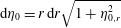 $\text{d}\unicode[STIX]{x1D702}_{0}=r\,\text{d}r\sqrt{1+\unicode[STIX]{x1D702}_{0,r}^{2}}$
, as detailed in appendix B. Furthermore, the left-hand side of (3.23) is non-zero because the kinematic and the contact line conditions are not homogeneous at second order:
 $$\begin{eqnarray}\langle \boldsymbol{q}^{\dagger },(\text{i}\unicode[STIX]{x1D714}{\mathcal{B}}-{\mathcal{A}})\hat{\boldsymbol{q}}_{2}\rangle =\underbrace{\langle (\text{i}\unicode[STIX]{x1D714}^{\dagger }{\mathcal{B}}^{\dagger }-{\mathcal{A}}^{\dagger })\boldsymbol{q}^{\dagger },\hat{\boldsymbol{q}}_{2}\rangle }_{=0}+\int _{\unicode[STIX]{x1D702}_{0}}\overline{\unicode[STIX]{x1D6F7}}^{\dagger }{\displaystyle \frac{\text{d}A\unicode[STIX]{x1D702}_{1}^{A}}{\text{d}T}}\,\text{d}\unicode[STIX]{x1D702}_{0}-{\displaystyle \frac{\sin ^{3}\unicode[STIX]{x1D703}_{s}}{Bo}}\overline{\unicode[STIX]{x1D702}}^{\dagger }\left.{\displaystyle \frac{\unicode[STIX]{x2202}\hat{\unicode[STIX]{x1D702}}_{2}}{\unicode[STIX]{x2202}r}}\right|_{r=1},\end{eqnarray}$$
where the integral on the free surface
 $\unicode[STIX]{x1D702}_{0}$
comes from the slow time derivative in the second-order kinematic condition (3.18), and the last term is associated with the contact line model. The detailed calculation yielding these boundary and corner terms is reported in appendix B.
At this point, the nonlinear contact angle correction due to the contact line model enters in the analysis through the geometrical relation
 $$\begin{eqnarray}\left.{\displaystyle \frac{\unicode[STIX]{x2202}\unicode[STIX]{x1D702}_{2}}{\unicode[STIX]{x2202}r}}\right|_{r=1}={\displaystyle \frac{-\unicode[STIX]{x1D703}_{2}}{\sin ^{2}(\unicode[STIX]{x1D703}_{s})}},\end{eqnarray}$$
with
 $$\begin{eqnarray}\unicode[STIX]{x1D703}_{2}+O(\unicode[STIX]{x1D716})=\left.\hat{\unicode[STIX]{x1D6FC}}{\displaystyle \frac{\unicode[STIX]{x2202}\unicode[STIX]{x1D702}_{1}}{\unicode[STIX]{x2202}t}}\right|_{r=1}+\left.{\displaystyle \frac{\hat{\unicode[STIX]{x1D6E5}}}{2}}\tanh \left(\unicode[STIX]{x1D6FD}Ca\unicode[STIX]{x1D716}{\displaystyle \frac{\unicode[STIX]{x2202}\unicode[STIX]{x1D702}_{1}}{\unicode[STIX]{x2202}t}}\right)\right|_{r=1},\end{eqnarray}$$
where
 $\hat{\unicode[STIX]{x1D6E5}}$
is the rescaled hysteresis range,
 $\unicode[STIX]{x1D6E5}=\unicode[STIX]{x1D716}^{2}\hat{\unicode[STIX]{x1D6E5}}$
, and
 $\hat{\unicode[STIX]{x1D6FC}}$
is the rescaled slip coefficient,
 $\unicode[STIX]{x1D6FC}Ca=\unicode[STIX]{x1D716}\hat{\unicode[STIX]{x1D6FC}}$
. In the following we derive the solutions coming from the two possible scalings of the steepness coefficient
 $\unicode[STIX]{x1D6FD}$
introduced in (3.1).
3.4 Amplitude equation: case I,
$\unicode[STIX]{x1D6FD}Ca=\hat{\unicode[STIX]{x1D6FD}}/\unicode[STIX]{x1D716}$

In this case the second-order contact line law (3.27) reads
 $$\begin{eqnarray}\unicode[STIX]{x1D703}_{2}=\left.\hat{\unicode[STIX]{x1D6FC}}{\displaystyle \frac{\unicode[STIX]{x2202}\unicode[STIX]{x1D702}_{1}}{\unicode[STIX]{x2202}t}}\right|_{r=1}+\left.{\displaystyle \frac{\hat{\unicode[STIX]{x1D6E5}}}{2}}\tanh \left(\hat{\unicode[STIX]{x1D6FD}}{\displaystyle \frac{\unicode[STIX]{x2202}\unicode[STIX]{x1D702}_{1}}{\unicode[STIX]{x2202}t}}\right)\right|_{r=1}.\end{eqnarray}$$
In order to impose a compatibility condition in (3.25), which is needed to determine the amplitude
 $A(T)$
in (3.14), the terms oscillating at the natural frequency in the contact line model (3.28) have to be considered, as done for the dynamic and kinematic conditions (3.17), (3.18). However, the
 $\tanh$
function is nonlinear and not purely harmonic, but through the Fourier series its
 $\unicode[STIX]{x1D714}$
harmonic may be isolated (see Nayfeh Reference Nayfeh2008):
 $$\begin{eqnarray}\left.\tanh \left(\hat{\unicode[STIX]{x1D6FD}}{\displaystyle \frac{\unicode[STIX]{x2202}\unicode[STIX]{x1D702}_{1}}{\unicode[STIX]{x2202}t}}\right)\right|_{r=1}=\tanh \left(\hat{\unicode[STIX]{x1D6FD}}\text{i}\unicode[STIX]{x1D714}A\unicode[STIX]{x1D702}_{1}^{A}|_{r=1}\text{e}^{\text{i}(\unicode[STIX]{x1D714}t+m\unicode[STIX]{x1D719})}+\text{c.c.}\right)=\mathop{\sum }_{k=-\infty }^{\infty }d_{k}(\unicode[STIX]{x1D719})\text{e}^{\text{i}k\unicode[STIX]{x1D714}t}.\end{eqnarray}$$
The complex amplitude and
 $\unicode[STIX]{x1D702}_{1}^{A}$
can be decomposed in modulus and phase, namely
 $A(T)=|A(T)|\text{e}^{\text{i}\unicode[STIX]{x1D717}(T)}$
and
 $\unicode[STIX]{x1D702}_{1}^{A}=|\unicode[STIX]{x1D702}_{1}^{A}|\text{e}^{\text{i}\unicode[STIX]{x1D717}_{\unicode[STIX]{x1D702}}}$
. By defining the variable
 $\unicode[STIX]{x1D709}=\unicode[STIX]{x1D714}t+m\unicode[STIX]{x1D719}+\unicode[STIX]{x03C0}/2+\unicode[STIX]{x1D717}_{\unicode[STIX]{x1D702}}|_{r=1}+\unicode[STIX]{x1D717}(T)$
, the coefficient
 $d_{k}$
is given by
 $$\begin{eqnarray}\displaystyle d_{k}(\unicode[STIX]{x1D719}) & = & \displaystyle {\displaystyle \frac{\unicode[STIX]{x1D714}}{2\unicode[STIX]{x03C0}}}\int _{-\unicode[STIX]{x03C0}/\unicode[STIX]{x1D714}}^{\unicode[STIX]{x03C0}/\unicode[STIX]{x1D714}}\tanh (\hat{\unicode[STIX]{x1D6FD}}\unicode[STIX]{x1D714}|A||\unicode[STIX]{x1D702}_{1}^{A}|_{r=1}|2\cos (\unicode[STIX]{x1D709}))\text{e}^{-\text{i}k\unicode[STIX]{x1D714}t}\,\text{d}t\nonumber\\ \displaystyle & = & \displaystyle \text{e}^{\text{i}k(m\unicode[STIX]{x1D719}+\unicode[STIX]{x03C0}/2+\unicode[STIX]{x1D717}_{\unicode[STIX]{x1D702}}+\unicode[STIX]{x1D717}(T))}\underbrace{{\displaystyle \frac{1}{2\unicode[STIX]{x03C0}}}\int _{-\unicode[STIX]{x03C0}}^{\unicode[STIX]{x03C0}}\tanh (\hat{\unicode[STIX]{x1D6FD}}\unicode[STIX]{x1D714}|A||\unicode[STIX]{x1D702}_{1}^{A}|_{r=1}|2\cos (\unicode[STIX]{x1D709}))\text{e}^{-\text{i}k\unicode[STIX]{x1D709}}\,\text{d}\unicode[STIX]{x1D709}}_{{\displaystyle \frac{2}{\unicode[STIX]{x03C0}}}c_{k}(|A|)},\end{eqnarray}$$
where the prefactor
 $2/\unicode[STIX]{x03C0}$
has been introduced to simplify the upcoming analysis and the Fourier coefficient
 $c_{k}(|A|)$
is only a function of the amplitude magnitude
 $|A|$
since
 $\hat{\unicode[STIX]{x1D6FD}}$
is set by the contact line law and
 $\unicode[STIX]{x1D714}$
and
 $|\unicode[STIX]{x1D702}_{1}^{A}|_{r=1}$
by the first-order problem. Consequently, the nonlinear term reads
 $$\begin{eqnarray}\displaystyle \left.\tanh \left(\hat{\unicode[STIX]{x1D6FD}}{\displaystyle \frac{\unicode[STIX]{x2202}\unicode[STIX]{x1D702}_{1}}{\unicode[STIX]{x2202}t}}\right)\right|_{r=1} & = & \displaystyle {\displaystyle \frac{2}{\unicode[STIX]{x03C0}}}\mathop{\sum }_{k=-\infty }^{\infty }c_{k}(|A|)\text{e}^{\text{i}k\unicode[STIX]{x1D709}}\nonumber\\ \displaystyle & = & \displaystyle {\displaystyle \frac{2}{\unicode[STIX]{x03C0}}}c_{1}(|A|)\text{e}^{\text{i}(\unicode[STIX]{x1D714}t+m\unicode[STIX]{x1D719}+\unicode[STIX]{x03C0}/2+\unicode[STIX]{x1D717}_{\unicode[STIX]{x1D702}}|_{r=1}+\unicode[STIX]{x1D717}(T))}+\text{c.c.}+\text{NRT},\end{eqnarray}$$
where we have isolated the harmonic oscillating at the sloshing natural frequency. The Fourier coefficient
 $c_{1}(|A|)$
can be computed numerically. It varies between the limiting value
 $1$
at large amplitude and
 $0$
when
 $|A|$
is small. As anticipated above, the exact shape of the function
 $c_{1}(|A|)$
depends on the first-order problem and has to be recomputed when the oscillation frequency
 $\unicode[STIX]{x1D714}$
or the rescaled steepness coefficient
 $\hat{\unicode[STIX]{x1D6FD}}$
are changed. A typical curve of
 $c_{1}(|A|)$
for the reference case introduced in § 3.2 is shown by the solid line in figure 5.
The first Fourier coefficient
 $c_{1}(|A|)$
of the nonlinear term in the second-order contact line model (3.27) shown as a function of the oscillation amplitude
 $|A|$
in the case of
 $Bo=500$
,
 $\unicode[STIX]{x1D703}_{s}=\unicode[STIX]{x03C0}/4$
(so that
 $\unicode[STIX]{x1D714}=1.35$
) and
 $\hat{\unicode[STIX]{x1D6FD}}=1$
. The solid line corresponds to case I (
 $Ca\unicode[STIX]{x1D6FD}=\hat{\unicode[STIX]{x1D6FD}}/\unicode[STIX]{x1D716}$
) whereas case II (
 $Ca\unicode[STIX]{x1D6FD}=\hat{\unicode[STIX]{x1D6FD}}/\unicode[STIX]{x1D716}^{2}$
) is shown by the dashed line.

Substituting equation (3.31) in the
 $\unicode[STIX]{x1D716}$
-order contact line model (3.26) yields
 $$\begin{eqnarray}\left.{\displaystyle \frac{\unicode[STIX]{x2202}\unicode[STIX]{x1D702}_{2}}{\unicode[STIX]{x2202}r}}\right|_{r=1}=\left.-{\displaystyle \frac{\hat{\unicode[STIX]{x1D6FC}}}{\sin ^{2}(\unicode[STIX]{x1D703}_{s})}}\text{i}\unicode[STIX]{x1D714}\unicode[STIX]{x1D702}_{1}^{A}|_{r=1}A\text{e}^{\text{i}\unicode[STIX]{x1D714}t}\text{e}^{\text{i}m\unicode[STIX]{x1D719}}-{\displaystyle \frac{\text{i}\hat{\unicode[STIX]{x0394}}c_{1}(|A|)}{\unicode[STIX]{x03C0}\sin ^{2}(\unicode[STIX]{x1D703}_{s})}}{\displaystyle \frac{\unicode[STIX]{x1D702}_{1}^{A}|_{r=1}}{|\unicode[STIX]{x1D702}_{1}^{A}|_{r=1}|}}{\displaystyle \frac{A}{|A|}}\text{e}^{\text{i}\unicode[STIX]{x1D714}t}\text{e}^{\text{i}m\unicode[STIX]{x1D719}}\right|_{r=1}+\text{c.c.}+\text{NRT},\end{eqnarray}$$
where the first term on the right-hand side is associated with the linear part of the contact line model (2.5) and provides a correction to the dynamic contact angle, found proportional to the contact line velocity. The second term on the right-hand side is nonlinear with respect to the contact line velocity. Its origin is attributed to the fast dynamic hysteresis, proportional to the rescaled hysteresis range
 $\hat{\unicode[STIX]{x1D6E5}}$
. Introducing the auxiliary constant
 $\unicode[STIX]{x1D705}$
and the two real damping coefficients
 $\unicode[STIX]{x1D701}$
and
 $\unicode[STIX]{x1D712}$
, defined as
 $$\begin{eqnarray}\displaystyle \unicode[STIX]{x1D705}=(\overline{\unicode[STIX]{x1D702}}^{\dagger }\unicode[STIX]{x1D702}_{1}^{A})_{r=1}\bigg/\int _{\unicode[STIX]{x1D702}_{0}}\overline{\unicode[STIX]{x1D702}}^{\dagger }\unicode[STIX]{x1D6F7}_{1}^{A}+\overline{\unicode[STIX]{x1D6F7}}^{\dagger }\unicode[STIX]{x1D702}_{1}^{A}\,\text{d}\unicode[STIX]{x1D702}_{0},\quad \unicode[STIX]{x1D701}={\displaystyle \frac{-\text{i}\unicode[STIX]{x1D714}\sin (\unicode[STIX]{x1D703}_{s})\hat{\unicode[STIX]{x1D6FC}}\unicode[STIX]{x1D705}}{Bo}},\quad \unicode[STIX]{x1D712}={\displaystyle \frac{-\text{i}\sin (\unicode[STIX]{x1D703}_{s})\hat{\unicode[STIX]{x0394}}\unicode[STIX]{x1D705}}{\unicode[STIX]{x03C0}Bo|\unicode[STIX]{x1D702}_{1}^{A}|_{r=1}}}, & & \displaystyle \nonumber\\ \displaystyle & & \displaystyle\end{eqnarray}$$
the substitution of expression (3.32) in (3.25) yields the compatibility condition
 $$\begin{eqnarray}\displaystyle {\displaystyle \frac{\text{d}A}{\text{d}T}}+\unicode[STIX]{x1D701}A+\unicode[STIX]{x1D712}c_{1}(|A|){\displaystyle \frac{A}{|A|}}=0, & & \displaystyle\end{eqnarray}$$
where the last term corresponds to the function
 $c_{1}(|A|)$
multiplying the sign of
 $A$
. Since the function
 $c_{1}(|A|)$
is real, decomposing the complex amplitude in modulus and phase,
 $A(T)=|A(T)|\text{e}^{\text{i}\unicode[STIX]{x1D717}(T)}$
,
 $$\begin{eqnarray}\displaystyle {\displaystyle \frac{\text{d}\unicode[STIX]{x1D717}}{\text{d}T}}=0. & & \displaystyle\end{eqnarray}$$
From equation (3.35) we argue that the sloshing frequency is not modified at leading order and that the amplitude phase
 $\unicode[STIX]{x1D717}(T)$
is set by the initial condition
 $\unicode[STIX]{x1D717}(T)=\unicode[STIX]{x1D717}_{0}$
. The value of
 $|A|$
as a function of time, which dictates the relaxation dynamics caused by the contact line dissipation, can be obtained by numerical integration of (3.34). The corresponding contact line motion that accounts for the weakly nonlinear correction is
 $$\begin{eqnarray}\displaystyle \unicode[STIX]{x1D702}_{1}|_{r=1}=2|A(T)||\unicode[STIX]{x1D702}_{1}^{A}|_{r=1}\cos (\unicode[STIX]{x1D714}t+\unicode[STIX]{x1D717}_{0}+m\unicode[STIX]{x1D719}+\unicode[STIX]{x1D717}_{\unicode[STIX]{x1D702}}|_{r=1}). & & \displaystyle\end{eqnarray}$$
Specifically,
 $|A(T)|$
is the nonlinear correction on the amplitude, and
 $\unicode[STIX]{x1D717}_{\unicode[STIX]{x1D702}}$
is the phase of
 $\unicode[STIX]{x1D702}_{1|_{r=1}}^{A}$
, which is nil due to the way the eigenmode
 $\boldsymbol{q}_{1}^{A}$
has been normalized. It should be noted that
 $\unicode[STIX]{x1D702}_{1}^{A}$
,
 $\unicode[STIX]{x1D717}_{\unicode[STIX]{x1D702}}$
and
 $A(T)$
all depend on the normalization of the direct mode, although the final result
 $\unicode[STIX]{x1D702}_{1}$
does not.
Contact line motion (blue line) modulated by the slow time amplitude (red line) of the fundamental free-end edge sloshing mode,
 $m=1$
, following an initial deflection of the interface of amplitude,
 $Z_{0}=\unicode[STIX]{x1D716}A_{0}=0.1$
, from rest (
 $\unicode[STIX]{x1D717}_{0}=0$
). The Bond number and the static contact angle are equal to
 $Bo=500$
and
 $\unicode[STIX]{x1D703}_{s}=\unicode[STIX]{x03C0}/4$
, and the contact line model parameters are set to
 $Ca=0.01$
,
 $\unicode[STIX]{x1D6FC}=60\text{ rad}$
,
 $\unicode[STIX]{x1D6E5}=20^{\circ }$
and
 $\hat{\unicode[STIX]{x1D6FD}}=6.5$
. The steepness of the contact angle hysteresis is equal to (a) case I (
 $Ca\unicode[STIX]{x1D6FD}=\hat{\unicode[STIX]{x1D6FD}}/\unicode[STIX]{x1D716}$
) and (b) case II (
 $Ca\unicode[STIX]{x1D6FD}=\hat{\unicode[STIX]{x1D6FD}}/\unicode[STIX]{x1D716}^{2}$
).

We consider, as an illustrative example, the dynamics of the fundamental sloshing mode,
 $m=1$
, following an initial deflection of the interface of amplitude
 $Z_{0}=\unicode[STIX]{x1D716}A_{0}=0.1$
from rest (
 $\unicode[STIX]{x1D717}_{0}=0$
) for the set of representative parameters chosen throughout this section. The Bond number and the static contact angle are equal to
 $Bo=500$
and
 $\unicode[STIX]{x1D703}_{s}=\unicode[STIX]{x03C0}/4$
, and the contact line model parameters are set to
 $Ca=0.01$
,
 $\unicode[STIX]{x1D6FC}=60\text{ rad}$
,
 $\unicode[STIX]{x1D6E5}=20^{\circ }$
and
 $\hat{\unicode[STIX]{x1D6FD}}=1$
. Figure 6(a) shows the second-order contact line motion (blue line) and
 $|A(T)|$
(red line). As inferred from (3.35) we find that the sloshing frequency is not modified by capillary effects. The amplitude contrasts with the first-order solution (figure 4
c). The contact line is significantly damped: the wave amplitude is more than a hundred times smaller than the initial amplitude of our reference case after forty periods. According to the amplitude equation (3.34) the effective damping appears as the sum of two terms: a linear contribution, weighted by the linear damping coefficient
 $\unicode[STIX]{x1D701}$
, resulting from the linear part of the contact line model, and a contribution, scaled by the nonlinear damping coefficient
 $\unicode[STIX]{x1D712}$
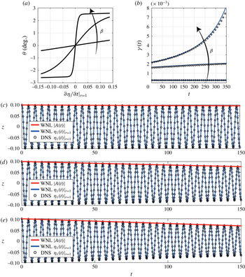
, originating from the dynamic contact line hysteresis at small velocity. This last contribution is nonlinear in nature. We refer the interested reader to appendix C for a validation of the asymptotic analysis against direct numerical simulation of the governing equations. Let us now consider another distinguished limit of the steepness coefficient
 $\unicode[STIX]{x1D6FD}Ca$
(case II) before deepening the discussion of capillary damping effects.
3.5 Amplitude equation: case II,
$\unicode[STIX]{x1D6FD}Ca=\hat{\unicode[STIX]{x1D6FD}}/\unicode[STIX]{x1D716}^{2}$

When the steepness factor
 $\unicode[STIX]{x1D6FD}$
is larger,
 $\unicode[STIX]{x1D6FD}Ca=\hat{\unicode[STIX]{x1D6FD}}/\unicode[STIX]{x1D716}^{2}$
, the second-order contact line law (3.27) reads
 $$\begin{eqnarray}\unicode[STIX]{x1D703}_{2}+O(\unicode[STIX]{x1D716})=\left.\hat{\unicode[STIX]{x1D6FC}}{\displaystyle \frac{\unicode[STIX]{x2202}\unicode[STIX]{x1D702}_{1}}{\unicode[STIX]{x2202}t}}\right|_{r=1}+\left.{\displaystyle \frac{\hat{\unicode[STIX]{x1D6E5}}}{2}}\tanh \left({\displaystyle \frac{\hat{\unicode[STIX]{x1D6FD}}}{\unicode[STIX]{x1D716}}}{\displaystyle \frac{\unicode[STIX]{x2202}\unicode[STIX]{x1D702}_{1}}{\unicode[STIX]{x2202}t}}\right)\right|_{r=1}.\end{eqnarray}$$
We need to isolate the resonating term in the nonlinear boundary condition in order to impose a compatibility condition in (3.25). By taking the Fourier transform of the nonlinear term in (3.37) we obtain
 $$\begin{eqnarray}\left.\tanh \left({\displaystyle \frac{\hat{\unicode[STIX]{x1D6FD}}}{\unicode[STIX]{x1D716}}}{\displaystyle \frac{\unicode[STIX]{x2202}\unicode[STIX]{x1D702}_{1}}{\unicode[STIX]{x2202}t}}\right)\right|_{r=1}=\tanh \left({\displaystyle \frac{\hat{\unicode[STIX]{x1D6FD}}}{\unicode[STIX]{x1D716}}}\text{i}\unicode[STIX]{x1D714}A\unicode[STIX]{x1D702}_{1}^{A}|_{r=1}\text{e}^{\text{i}(\unicode[STIX]{x1D714}t+m\unicode[STIX]{x1D719})}+\text{c.c.}\right)=\mathop{\sum }_{k=-\infty }^{\infty }d_{k}(\unicode[STIX]{x1D719})\text{e}^{\text{i}k\unicode[STIX]{x1D714}t}.\end{eqnarray}$$
The complex amplitude and
 $\unicode[STIX]{x1D702}_{1}^{A}$
can be decomposed in modulus and phase, namely
 $A(T)=|A(T)|\text{e}^{\text{i}\unicode[STIX]{x1D717}(T)}$
and
 $\unicode[STIX]{x1D702}_{1}^{A}=|\unicode[STIX]{x1D702}_{1}^{A}|\text{e}^{\text{i}\unicode[STIX]{x1D717}_{\unicode[STIX]{x1D702}}}$
. Using the variable
 $\unicode[STIX]{x1D709}=\unicode[STIX]{x1D714}t+m\unicode[STIX]{x1D719}+\unicode[STIX]{x03C0}/2+\unicode[STIX]{x1D717}_{\unicode[STIX]{x1D702}}|_{r=1}+\unicode[STIX]{x1D717}(T)$
, the coefficients
 $d_{k}$
are here given by
 $$\begin{eqnarray}d_{k}(\unicode[STIX]{x1D719})={\displaystyle \frac{\unicode[STIX]{x1D714}}{2\unicode[STIX]{x03C0}}}\int _{-\unicode[STIX]{x03C0}/\unicode[STIX]{x1D714}}^{\unicode[STIX]{x03C0}/\unicode[STIX]{x1D714}}\tanh (\hat{\unicode[STIX]{x1D6FD}}/\unicode[STIX]{x1D716}\unicode[STIX]{x1D714}|A||\unicode[STIX]{x1D702}_{1}^{A}|_{r=1}2\cos (\unicode[STIX]{x1D709}))\text{e}^{-\text{i}k\unicode[STIX]{x1D714}t}\,\text{d}t.\end{eqnarray}$$
The hyperbolic tangent in the integrand can be expanded as the sum of the sign function plus a correction
 $f(\unicode[STIX]{x1D716},\unicode[STIX]{x1D709})$
, which satisfies
 $\int _{-\unicode[STIX]{x03C0}}^{\unicode[STIX]{x03C0}}f(\unicode[STIX]{x1D716},\unicode[STIX]{x1D709})\text{e}^{-\text{i}k\unicode[STIX]{x1D714}t}\,\text{d}\unicode[STIX]{x1D709}=O(\unicode[STIX]{x1D716})$
. Consequently, equation (3.39) reads
 $$\begin{eqnarray}\displaystyle d_{k}(\unicode[STIX]{x1D719}) & = & \displaystyle {\displaystyle \frac{\unicode[STIX]{x1D714}}{2\unicode[STIX]{x03C0}}}\int _{-\unicode[STIX]{x03C0}/\unicode[STIX]{x1D714}}^{\unicode[STIX]{x03C0}/\unicode[STIX]{x1D714}}\text{sgn}(\hat{\unicode[STIX]{x1D6FD}}/\unicode[STIX]{x1D716}\unicode[STIX]{x1D714}|A||\unicode[STIX]{x1D702}_{1}^{A}|_{r=1}2\cos (\unicode[STIX]{x1D709}))\text{e}^{-\text{i}k\unicode[STIX]{x1D714}t}\,\text{d}t+\underbrace{{\displaystyle \frac{\unicode[STIX]{x1D714}}{2\unicode[STIX]{x03C0}}}\int _{-\unicode[STIX]{x03C0}/\unicode[STIX]{x1D714}}^{\unicode[STIX]{x03C0}/\unicode[STIX]{x1D714}}f(\unicode[STIX]{x1D716},\unicode[STIX]{x1D709})\text{e}^{-\text{i}k\unicode[STIX]{x1D714}t}\,\text{d}t}_{O(\unicode[STIX]{x1D716})}\nonumber\\ \displaystyle & = & \displaystyle \text{e}^{\text{i}k(m\unicode[STIX]{x1D719}+\unicode[STIX]{x03C0}/2+\unicode[STIX]{x1D717}_{\unicode[STIX]{x1D702}}|_{r=1}+\unicode[STIX]{x1D717}(T))}\underbrace{{\displaystyle \frac{1}{2\unicode[STIX]{x03C0}}}\int _{-\unicode[STIX]{x03C0}}^{\unicode[STIX]{x03C0}}\text{sgn}(\cos (\unicode[STIX]{x1D709}))\text{e}^{-\text{i}k\unicode[STIX]{x1D709}}\,\text{d}\unicode[STIX]{x1D709}}_{\frac{2}{\unicode[STIX]{x03C0}}c_{k}}+O(\unicode[STIX]{x1D716}),\end{eqnarray}$$
which further gives
 $$\begin{eqnarray}\left.\tanh \left({\displaystyle \frac{\hat{\unicode[STIX]{x1D6FD}}}{\unicode[STIX]{x1D716}}}{\displaystyle \frac{\unicode[STIX]{x2202}\unicode[STIX]{x1D702}_{1}}{\unicode[STIX]{x2202}t}}\right)\right|_{r=1}={\displaystyle \frac{2}{\unicode[STIX]{x03C0}}}\mathop{\sum }_{k=-\infty }^{\infty }c_{k}\text{e}^{\text{i}k\unicode[STIX]{x1D709}}={\displaystyle \frac{2}{\unicode[STIX]{x03C0}}}c_{1}\text{e}^{\text{i}(\unicode[STIX]{x1D714}t+m\unicode[STIX]{x1D719}+\unicode[STIX]{x03C0}/2+\unicode[STIX]{x1D717}_{\unicode[STIX]{x1D702}}|_{r=1}+\unicode[STIX]{x1D717}(T))}+\text{c.c.}+O(\unicode[STIX]{x1D716})+\text{NRT},\end{eqnarray}$$
where we have isolated the harmonic oscillating at the sloshing natural frequency and
 $\text{NRT}$
denotes the non-resonating terms. The Fourier coefficient
 $c_{1}$
does not depend here on the amplitude and is equal to
 $$\begin{eqnarray}{\displaystyle \frac{2}{\unicode[STIX]{x03C0}}}c_{1}={\displaystyle \frac{1}{2\unicode[STIX]{x03C0}}}\int _{-\unicode[STIX]{x03C0}}^{\unicode[STIX]{x03C0}}\text{sgn}(\cos (\unicode[STIX]{x1D709}))\text{e}^{-\text{i}\unicode[STIX]{x1D709}}\,\text{d}\unicode[STIX]{x1D709}={\displaystyle \frac{2}{\unicode[STIX]{x03C0}}},\quad \Rightarrow c_{1}=1.\end{eqnarray}$$
Injecting equation (3.41) into the geometrical relation (3.37) and substituting in (3.26), one gets
 $$\begin{eqnarray}\left.{\displaystyle \frac{\unicode[STIX]{x2202}\unicode[STIX]{x1D702}_{2}}{\unicode[STIX]{x2202}r}}\right|_{r=1}=\left.-{\displaystyle \frac{\hat{\unicode[STIX]{x1D6FC}}}{\sin ^{2}(\unicode[STIX]{x1D703}_{s})}}\text{i}\unicode[STIX]{x1D714}\unicode[STIX]{x1D702}_{1}^{A}|_{r=1}A\text{e}^{\text{i}\unicode[STIX]{x1D714}t}\text{e}^{\text{i}m\unicode[STIX]{x1D719}}-{\displaystyle \frac{\text{i}\hat{\unicode[STIX]{x1D6E5}}}{\unicode[STIX]{x03C0}\sin ^{2}(\unicode[STIX]{x1D703}_{s})}}{\displaystyle \frac{\unicode[STIX]{x1D702}_{1}^{A}|_{r=1}}{|\unicode[STIX]{x1D702}_{1}^{A}|_{r=1}|}}{\displaystyle \frac{A}{|A|}}\text{e}^{\text{i}\unicode[STIX]{x1D714}t}\text{e}^{\text{i}m\unicode[STIX]{x1D719}}\right|_{r=1}+\text{c.c.}+\text{NRT}.\end{eqnarray}$$
As in case I we can distinguish a linear term on the right-hand side and a nonlinear term attributed to the fast variation of the hysteresis range at small contact line velocity. Specifically, this term only depends on the phase of the velocity, a result consistent with the use of the
 $\text{sgn}$
function (which only depends on the sign of its argument). As a result, this term provides a different correction depending on whether the interface is advancing or receding.
Substituting (3.43) in (3.25) yields the compatibility condition
 $$\begin{eqnarray}{\displaystyle \frac{\text{d}A}{\text{d}T}}+\unicode[STIX]{x1D701}A+\unicode[STIX]{x1D712}{\displaystyle \frac{A}{|A|}}=0,\end{eqnarray}$$
where the last term on the left-hand side corresponds to the sign of
 $A$
and where
 $\unicode[STIX]{x1D701}$
and
 $\unicode[STIX]{x1D712}$
have been defined in (3.33). Similarly to (3.34), the effective damping appears as the sum of a linear contribution, weighted by the linear damping coefficient
 $\unicode[STIX]{x1D701}$
, resulting from the linear part of the contact line model and a nonlinear contribution, scaled by the nonlinear damping coefficient
 $\unicode[STIX]{x1D712}$
, originating in the contact line hysteresis.
Decomposing the complex amplitude in modulus and phase,
 $A(T)=|A(T)|\text{e}^{\text{i}\unicode[STIX]{x1D717}(T)}$
, equation (3.44) may be integrated analytically:
 $$\begin{eqnarray}|A(T)|=\left(A_{0}+{\displaystyle \frac{\unicode[STIX]{x1D712}}{\unicode[STIX]{x1D701}}}\right)\text{e}^{-\unicode[STIX]{x1D701}T}-{\displaystyle \frac{\unicode[STIX]{x1D712}}{\unicode[STIX]{x1D701}}},\unicode[STIX]{x1D717}(T)=\unicode[STIX]{x1D717}_{0},\end{eqnarray}$$
where
 $A_{0}$
and
 $\unicode[STIX]{x1D717}_{0}$
depend on the initial conditions. Equation (3.45) represents the weakly nonlinear correction to the first-order solution (3.14) associated with the contact line model (2.5), yielding the contact line motion (3.36).
The second-order contact line motion following an initial deflection of amplitude
 $Z_{0}=\unicode[STIX]{x1D716}A_{0}=0.1$
is shown in figure 6(b). The same set of parameters used for figure 6(a) is used, except for the steepness factor
 $Ca\unicode[STIX]{x1D6FD}$
, which is now taken equal to
 $1/\unicode[STIX]{x1D716}^{2}$
(
 $\hat{\unicode[STIX]{x1D6FD}}=1$
). Similarly to case I, the contact line motion is found to be damped by capillarity. However, the wave attenuation in (b) is faster than in (a) where the oscillation still persists for
 $t>200$
. In contrast, in case II, the wave amplitude is seen to decrease abruptly in a linear fashion at the end of the motion (see (3.45)), yielding a finite time arrest: the oscillating motion is nil for sufficiently large time. These features are discussed in the upcoming section.
4 Discussion
Our multiple scale analysis has revealed the nonlinear nature of sloshing when dynamic capillary hysteresis is included. In this section, we discuss the dynamics of the fundamental sloshing mode, focusing on the wave attenuation:
 $$\begin{eqnarray}\unicode[STIX]{x1D6FE}(t)=-{\displaystyle \frac{\text{d}\log (|A(\unicode[STIX]{x1D716}t)|/A_{0})}{\text{d}t}}=-{\displaystyle \frac{\unicode[STIX]{x1D716}}{|A(T)|}}{\displaystyle \frac{\text{d}|A(T)|}{\text{d}T}},\end{eqnarray}$$
which corresponds to the derivative of the logarithmic decrement shown in figure 7(a).
(a) Amplitude modulation in logarithmic scale versus time and (b) capillary damping rate versus the wave amplitude of the fundamental free-end edge sloshing mode,
 $m=1$
, following an initial deflection
 $Z_{0}=\unicode[STIX]{x1D716}A_{0}=0.1$
. The Bond number and the static contact angle are equal to
 $Bo=500$
and
 $\unicode[STIX]{x1D703}_{s}=\unicode[STIX]{x03C0}/4$
, and the contact line model parameters are set to
 $Ca=0.01$
,
 $\unicode[STIX]{x1D6FC}=60\text{ rad}$
,
 $\unicode[STIX]{x1D6E5}=20^{\circ }$
and
 $\hat{\unicode[STIX]{x1D6FD}}=6.5$
. The steepness of the dynamic contact angle hysteresis at small contact line velocity is equal to
 $Ca\unicode[STIX]{x1D6FD}=\hat{\unicode[STIX]{x1D6FD}}/\unicode[STIX]{x1D716}$
for case I (solid line) and
 $Ca\unicode[STIX]{x1D6FD}=\hat{\unicode[STIX]{x1D6FD}}/\unicode[STIX]{x1D716}^{2}$
for case II (black dashed line). The red vertical line depicts the finite time at which the amplitude goes to zero in case I.

4.1 Case I:
$\unicode[STIX]{x1D6FD}Ca=\hat{\unicode[STIX]{x1D6FD}}/\unicode[STIX]{x1D716}$

Substituting the amplitude equation (3.34) in the instantaneous damping rate definition (4.1), we get
 $$\begin{eqnarray}\unicode[STIX]{x1D6FE}(t)=\unicode[STIX]{x1D716}\unicode[STIX]{x1D701}+\unicode[STIX]{x1D716}\unicode[STIX]{x1D712}{\displaystyle \frac{c_{1}(|A|)}{|A(\unicode[STIX]{x1D716}t)|}},\end{eqnarray}$$
as shown in figure 7(b) (solid line). The wave attenuation is not constant during sloshing and the instantaneous damping rate depends on the wave amplitude. For sufficiently large amplitude, such that
 $c_{1}(|A|)$
tends to one, the decay is practically exponential with damping rate approaching the limiting value
 $$\begin{eqnarray}\unicode[STIX]{x1D6FE}(t=0)=\unicode[STIX]{x1D716}\unicode[STIX]{x1D701}+\unicode[STIX]{x1D716}^{2}{\displaystyle \frac{\unicode[STIX]{x1D712}}{Z_{0}}}.\end{eqnarray}$$
Two contributions to the damping rate thus prevail at initial times: (i) one associated with the linear contact line friction, which is here proportional to
 $\unicode[STIX]{x1D6FC}$
, through
 $\unicode[STIX]{x1D701}$
, and (ii) a damping rate proportional to the hysteresis range
 $\unicode[STIX]{x1D6E5}$
, through
 $\unicode[STIX]{x1D712}$
, and inversely proportional to the initial amplitude
 $Z_{0}$
. Note that the second
 $1/Z_{0}$
contribution was found by Miles (Reference Miles1967) in the limit of small critical velocity, and assuming that the mean energy relaxes exponentially. Then the damping rate varies owing to the second term on the right-hand side of (4.2), which has an explicit dependence on
 $|A|$
. In particular, the numerator
 $c_{1}(|A|)$
varies slowly for intermediate amplitudes (see figure 5), whereas the denominator
 $|A|$
decreases linearly. Thus, the damping rate increases significantly when the sloshing amplitude decreases. However, at smaller oscillating amplitudes,
 $c_{1}(|A|)$
decreases linearly with respect to
 $|A|$
, with slope
 $c^{\prime }(0)=\text{d}c_{1}/\text{d}|A||_{|A|=0}$
, and the ratio
 $c_{1}/|A|$
tends to a constant value. As a consequence, the system enters in a low amplitude linear regime, with damping rate
 $$\begin{eqnarray}\unicode[STIX]{x1D6FE}(t=\infty )\rightarrow \unicode[STIX]{x1D716}\unicode[STIX]{x1D701}+\unicode[STIX]{x1D716}\unicode[STIX]{x1D712}c^{\prime }(0)=\unicode[STIX]{x1D716}\unicode[STIX]{x1D701}+\unicode[STIX]{x1D716}\unicode[STIX]{x1D712}\unicode[STIX]{x03C0}/2\hat{\unicode[STIX]{x1D6FD}}\unicode[STIX]{x1D714}|\unicode[STIX]{x1D702}_{1}^{A}|_{r=1},\end{eqnarray}$$
and the free-end edge mode decays exponentially.
4.2 Case II:
$\unicode[STIX]{x1D6FD}Ca=\hat{\unicode[STIX]{x1D6FD}}/\unicode[STIX]{x1D716}^{2}$

In the case of higher hysteresis steepness coefficient, the amplitude equation (3.44) yields
 $$\begin{eqnarray}\unicode[STIX]{x1D6FE}(t)=\unicode[STIX]{x1D716}\unicode[STIX]{x1D701}+\unicode[STIX]{x1D716}\unicode[STIX]{x1D712}{\displaystyle \frac{1}{|A(\unicode[STIX]{x1D716}t)|}},\end{eqnarray}$$
which is shown in figure 7(b) (dashed line). The wave attenuation is seen to depend on the wave amplitude. The decay is approximately exponential at large amplitude, and the damping rate is equal to that in (4.3). The wave attenuation then increases when the amplitude decreases. Rather than reaching a low amplitude linear regime the damping rate keeps increasing. In particular, we find the existence of a finite time
 $t^{\ast }$
such that the damping rate diverges:
 $$\begin{eqnarray}\unicode[STIX]{x1D6FE}(t=t^{\ast })\rightarrow \infty ,\end{eqnarray}$$
with
 $$\begin{eqnarray}t^{\ast }={\displaystyle \frac{1}{\unicode[STIX]{x1D716}\unicode[STIX]{x1D701}}}\log \left(1+{\displaystyle \frac{\unicode[STIX]{x1D701}}{\unicode[STIX]{x1D712}}}{\displaystyle \frac{Z_{0}}{\unicode[STIX]{x1D716}}}\right).\end{eqnarray}$$
The finite time singularity of the damping rate yields the arrest of the contact line, whose amplitude becomes exactly zero for
 $t=t^{\ast }$
(see (3.45)). Recalling that
 $\unicode[STIX]{x1D712}\propto \unicode[STIX]{x1D6E5}$
(3.3), we argue that the contact angle hysteresis at small contact line velocity is at the origin of this finite time arrest of the free-end edge mode. Consistent with this assertion we find that
 $t^{\ast }$
diverges if
 $\unicode[STIX]{x1D6E5}$
is set to zero. In this limit the system relaxes exponentially with damping rate
 $\unicode[STIX]{x1D716}\unicode[STIX]{x1D701}$
. Conversely, even a small value of the hysteresis range – as small as
 $1^{\circ }$
– is sufficient to induce a significant dissipative effect that, in turn, largely impacts the dynamics, and, in particular, leads to an arrest of free-end edge mode in finite time.
Finite time of arrest
 $t^{\ast }$
reported as a function of (a) the initial contact line displacement, (b) the slip coefficient, (c) the Bond number and (d) the static contact angle. The
 $+$
symbols displayed in (d) correspond to
 $t^{\ast }$
computed with a finer mesh (see appendix A), showing convergence with respect to grid resolution.

We now turn to investigating the parametric dependence of the time of arrest
 $t^{\ast }$
. To this end, we use the configuration introduced in § 3 as a reference and vary (i) the Bond number,
 $Bo$
, (ii) the static contact angle,
 $\unicode[STIX]{x1D703}_{s}$
, as well as (iii) the contact line model parameters,
 $\unicode[STIX]{x1D6FC}Ca$
and
 $\unicode[STIX]{x1D6E5}$
, and (iv) the set of the initial condition,
 $Z_{0}=\unicode[STIX]{x1D716}A_{0}$
. Using § 3, we anticipate that the first-order solution solely depends on
 $\unicode[STIX]{x1D703}_{s}$
and
 $Bo$
. The contact line model parameters
 $\unicode[STIX]{x1D6FC}Ca$
and
 $\unicode[STIX]{x1D6E5}$
, and the initial condition
 $A_{0}$
only enter the problem at second order. Using the definitions for
 $\unicode[STIX]{x1D701}$
and
 $\unicode[STIX]{x1D712}$
introduced in (4.7), we obtain a scaling law for
 $t^{\ast }$
:
 $$\begin{eqnarray}t^{\ast }\propto {\displaystyle \frac{Bo}{\unicode[STIX]{x1D714}\unicode[STIX]{x1D705}\sin (\unicode[STIX]{x1D703}_{s})}}{\displaystyle \frac{1}{\unicode[STIX]{x1D6FC}Ca}}\log \left(1+{\displaystyle \frac{\unicode[STIX]{x1D6FC}Ca\unicode[STIX]{x03C0}\unicode[STIX]{x1D714}}{\unicode[STIX]{x1D6E5}}}Z_{0}\right).\end{eqnarray}$$
In figure 8 we show the variation of
 $t^{\ast }$
as a function of the key parameters of the problem. The time of arrest evidently increases with the initial interface deflection,
 $Z_{0}$
, that sets the initial energy of the system, which must be dissipated to recover the rest configuration. A higher value of
 $Z_{0}$
thus requires a longer time before the interface comes back to rest. However, dependence of
 $t^{\ast }$
with respect to
 $Z_{0}$
is logarithmic (see (4.8)), such that the time of arrest increases less than linearly with
 $Z_{0}$
. Regarding the slip coefficient
 $\unicode[STIX]{x1D6FC}$
, an increase of its value yields an increase of the damping rate, and, in turn, a decrease of
 $t^{\ast }$
. This result remains true for all the values of
 $\unicode[STIX]{x1D6E5}$
considered (see figure 8
b). The frequency
 $\unicode[STIX]{x1D714}$
and the scalar quantity
 $\unicode[STIX]{x1D705}$
(introduced in (3.3)) both arise from the first-order problem. Consequently, they both depend on the static angle,
 $\unicode[STIX]{x1D703}_{s}$
, and the Bond number,
 $Bo$
, in a complex way. As a consequence, no scaling law for
 $t^{\ast }$
with
 $\unicode[STIX]{x1D703}_{s}$
and
 $Bo$
may be immediately deduced from (4.8) a priori. However, we have found numerically that both
 $\unicode[STIX]{x1D714}$
and
 $\unicode[STIX]{x1D705}$
do not vary significantly with
 $\unicode[STIX]{x1D703}_{s}$
and
 $Bo$
, respectively. In figure 8(c) the linear dependence of
 $t^{\ast }$
with
 $Bo$
is reported, whereas in Figure 8(d) we show that the time of arrest decreases when the static contact angle
 $\unicode[STIX]{x1D703}_{s}$
is increased. This aspect is corroborated by the ratio
 $Bo/\sin \unicode[STIX]{x1D703}_{s}$
in (4.8).
The dependence of
 $t^{\ast }$
on
 $Bo$
and
 $\unicode[STIX]{x1D703}_{s}$
may be rationalized when recalling that the dissipation,
 ${\mathcal{D}}$
, in a liquid wedge sliding on a solid substrate may be approximated in the following way (de Gennes et al.
Reference de Gennes, Brochard-Wyart and Quéré2002):
 $$\begin{eqnarray}{\mathcal{D}}\sim \unicode[STIX]{x1D70E}(\unicode[STIX]{x1D703}^{2}-\unicode[STIX]{x1D703}_{s}^{2})\sim {\displaystyle \frac{1}{Bo}}(\unicode[STIX]{x1D703}+\unicode[STIX]{x1D703}_{s})(\unicode[STIX]{x1D703}-\unicode[STIX]{x1D703}_{s}).\end{eqnarray}$$
The capillary-induced dissipation originates from the work of surface tension, which is non-zero only when the contact angle
 $\unicode[STIX]{x1D703}$
deviates from its equilibrium value
 $\unicode[STIX]{x1D703}_{s}$
. An increase in
 $Bo$
lowers the dissipation and thus increases
 $t^{\ast }$
. On the other hand, an increase in
 $\unicode[STIX]{x1D703}_{s}$
, while keeping constant the contact line model parameters, is positively correlated with the dissipation: increasing
 $\unicode[STIX]{x1D703}_{s}$
, while keeping constant
 $\unicode[STIX]{x1D6FC}$
and
 $\unicode[STIX]{x1D6E5}$
, merely translates upwards the plot in figure 1(b) yielding the contribution
 $\unicode[STIX]{x1D703}+\unicode[STIX]{x1D703}_{s}$
in (4.9) to increase while keeping constant
 $\unicode[STIX]{x1D703}-\unicode[STIX]{x1D703}_{s}$
.
Finally, from the relative position of the curves displayed in figure 8 obtained varying
 $\unicode[STIX]{x1D6E5}$
, we recover that an increase of
 $\unicode[STIX]{x1D6E5}$
always enhances the damping and lowers the value of
 $t^{\ast }$
, consistently with (4.8).
4.3 Comparison with the experiments of Cocciaro et al. (Reference Cocciaro, Faetti, Nobili and Festa1993)
We now compare the weakly nonlinear analysis with the experimental observations of Cocciaro et al. (Reference Cocciaro, Faetti, Nobili and Festa1993). Remarkably, these authors report careful measurements of the contact line dynamics. In particular, they measure the contact line elevation,
 $A_{c}$
according to their notation, and the dynamic contact angle,
 $\unicode[STIX]{x1D703}$
, versus the tilt angle at the axis,
 $\unicode[STIX]{x1D6FC}_{1}$
. With this information and the assumption of sinusoidal motion of the contact line, which is supported by experimental evidence, it is possible to derive the contact angle as a function of the contact line velocity that is here reported in figure 9(a). This behaviour well resembles the contact line law we have used in our analysis: a steep hysteresis range (of size
 $\unicode[STIX]{x1D6E5}=43^{\circ }$
) for small contact line velocity and an approximately linear dynamic range with
 $\unicode[STIX]{x1D6FC}_{a}\approx 100$
for advancing interface and
 $\unicode[STIX]{x1D6FC}_{r}\approx 200$
for the receding one. As previously discussed in the Introduction (§ 1), two different regimes are found by Cocciaro et al. (Reference Cocciaro, Faetti, Nobili and Festa1993): at higher amplitude the contact line slides on the solid substrate and the fluid interface well matches that of a free-edge mode. In contrast, at small amplitudes the pinned mode dominates the sloshing dynamics and the dynamic contact angle oscillates around its static value. The transition between the two regimes is evident when the damping rate is monitored; see figure 9(b) where the original data from Cocciaro et al. (Reference Cocciaro, Faetti, Nobili and Festa1993) are reproduced (solid line) as a function of the contact line amplitude,
 $A_{c}$
, rather than the amplitude of the tilt angle,
 $\unicode[STIX]{x1D6FC}_{1}$
, using their figure 3a for this conversion. When the wave amplitude is large (
 $A_{c}>2~\text{mm}$
) the damping rate increases for a decreasing amplitude of oscillation until it reaches a maximum value. Then, in the transition between the two regimes, the damping rate decreases until reaching a uniform value for the pinned motion, which is hardly visible in this representation (but clear in their figure 9
a).
(a) Contact line model corresponding to the experimental conditions of Cocciaro et al. (Reference Cocciaro, Faetti, Nobili and Festa1993) as can be deduced from figure 3 of their paper (solid line) and the contact line model used in this section (dashed line). (b) Dimensional capillary-induced damping rate over
 $\unicode[STIX]{x03C0}$
versus the contact line amplitude as measured by Cocciaro et al. (Reference Cocciaro, Faetti, Nobili and Festa1993) (solid line) at the container axis. The damping rate of the free-edge mode computed with the asymptotic analysis (dashed line) is computed using (4.5) and setting the physical parameters as in the experiment:
 $\unicode[STIX]{x1D703}_{s}=62^{\circ }$
,
 $Bo=346.4$
,
 $Ca=0.011$
and
 $\unicode[STIX]{x1D6E5}=43^{\circ }$
,
 $\unicode[STIX]{x1D6FC}=(\unicode[STIX]{x1D6FC}_{r}+\unicode[STIX]{x1D6FC}_{a})/2\approx 150$
. The damping rate due to the dissipation in the oscillating Stokes layer at the wall as found theoretically by Case & Parkinson (Reference Case and Parkinson1957) (see equation (4.10)), is shown by the red line.

As discussed above, our asymptotic analysis merely describes the dynamics of the free-edge mode that dominates the liquid sloshing in a circular container until the contact line starts to pin. A comparison with the experimental results of Cocciaro et al. (Reference Cocciaro, Faetti, Nobili and Festa1993) is then possibly restricted to the case of higher amplitude (
 $A_{c}>2~\text{mm}$
). With this aim, the damping rates computed with the asymptotic analysis are also shown in figure 9(b) (dashed line). Due to the steep contact angle hysteresis observed in the contact law in figure 9(a), the damping rates are calculated by using (4.5) (case II) and the other physical parameters are set as in the experiment:
 $\unicode[STIX]{x1D6E5}=43^{\circ }$
,
 $\unicode[STIX]{x1D6FC}=(\unicode[STIX]{x1D6FC}_{r}+\unicode[STIX]{x1D6FC}_{a})/2\approx 150$
,
 $\unicode[STIX]{x1D703}_{s}=62^{\circ }$
,
 $Bo=346.4$
and
 $Ca=0.011$
. Although the contact angle hysteresis,
 $\unicode[STIX]{x1D6E5}$
, and the slip coefficient,
 $\unicode[STIX]{x1D6FC}$
, are slightly larger with respect to the values allowed by the asymptotic machinery, the damping rates predicted by the asymptotic analysis (without any tuneable parameter) match well with those measured experimentally by Cocciaro et al. (Reference Cocciaro, Faetti, Nobili and Festa1993) in the high amplitude range (
 $A_{c}>2~\text{mm}$
). Conversely, our theory does not capture the decreasing of the damping rate for lower amplitudes (
 $A_{c}<2~\text{mm}$
).
We speculate that this discrepancy depends on the sticking of the interface at small amplitudes that requires the introduction of the pinned-edge mode to be described, which is not accounted for in our analysis. It has to be remarked, in fact, that the damping rate in the experiments was measured by measuring the tilt angle at the container’s axis,
 $\unicode[STIX]{x1D6FC}_{1}$
, where both free-edge and pinned modes are present, rather than at the contact line, where the pinned mode does not contribute. These two possible ways of measuring the wave decay are equivalent at large amplitudes but are different at small amplitude (see figure 3(a) of Cocciaro et al.
Reference Cocciaro, Faetti, Nobili and Festa1993). In particular, the damping rate measured at the contact line could have a diverging behaviour similar to that observed in our analysis since the contact line pins at a finite time and the free-edge mode expires.
In the same figure, we also show the viscous damping rate associated with the dissipation in the oscillating Stokes layers as found by the theory of Case & Parkinson (Reference Case and Parkinson1957):
 $$\begin{eqnarray}\unicode[STIX]{x1D6FE}_{\unicode[STIX]{x1D707}}={\displaystyle \frac{3.52}{2\unicode[STIX]{x03C0}}}{\displaystyle \frac{\sqrt{\unicode[STIX]{x1D708}}}{R^{3/4}g^{1/4}}}\unicode[STIX]{x1D714}.\end{eqnarray}$$
The viscous damping rate,
 $\unicode[STIX]{x1D6FE}_{\unicode[STIX]{x1D707}}$
(red line), significantly underestimates the wave decay at higher amplitude and does not depend on the oscillation amplitude of the free surface, in disagreement with experimental results. At small amplitude,
 $\unicode[STIX]{x1D6FE}_{\unicode[STIX]{x1D707}}$
is found to be close to the damping rate observed in the pinned regime, where the dissipation in the Stokes layer is no longer overshadowed by that in the dynamic meniscus.
5 Conclusions
We have presented a weakly nonlinear formulation for sloshing waves in a circular cylinder in partial wetting conditions. A nonlinear contact line model was incorporated into our asymptotic analysis as a boundary condition at the moving contact line. In particular, we have adopted a contact line model where a steep dynamic hysteresis range is married to the widely used Hocking law, which is a linear relation. In the limit of steep dynamic hysteresis this model mimics well the experimental observations in unidirectional flows where both static and dynamic hysteresis ranges are seen (Dussan Reference Dussan1979; Le Grand et al.
Reference Le Grand, Daerr and Limat2005; Rio et al.
Reference Rio, Daerr, Andreotti and Limat2005). In our asymptotic expansion, two distinguished solutions are considered depending on the steepness of the contact angle hysteresis that scales as
 $\unicode[STIX]{x1D6FD}Ca\sim \unicode[STIX]{x1D716}^{-1}$
(case I) or as
 $\unicode[STIX]{x1D6FD}Ca\sim \unicode[STIX]{x1D716}^{-2}$
(case II). In both cases, the zero-order problem consists of the static meniscus shape in the cylindrical geometry considered. At first order, the linear problem satisfied by the sloshing gravity–capillary waves is obtained. The resulting global modes are neutrally stable since no dissipation source is found at zero and first orders. Therefore, in the spirit of multiple scale analysis, a slowly varying amplitude and phase modulation are introduced at second order. They correspond to the weakly nonlinear correction accounting for capillary effects at the contact line.
The phase modulation is found not to enter at first order, so that capillary effects do not affect significantly the sloshing frequency. This result is in agreement with the experimental observations of Keulegan (Reference Keulegan1959) and Cocciaro et al. (Reference Cocciaro, Faetti, Nobili and Festa1993) where a weak dependence on the amplitude has been observed for the oscillation frequency in partial wetting conditions.
Capillary effects, however, have a dramatic influence on the damping rate: the amplitude modulation results in a significant attenuation of the first-order waves. According to the amplitude equations (3.34) and (3.44), capillary effects make two contributions to the damping rate: (i) a nonlinear contribution related to the contact angle hysteresis at small contact line velocities and (ii) a linear contribution imparted to the linear dependence between the contact angle and the contact line velocity. In our analysis, the capillary-induced damping rate is found to depend on the wave amplitude. This fact is consistent with the experimental observations of Keulegan (Reference Keulegan1959) and Cocciaro et al. (Reference Cocciaro, Faetti, Nobili and Festa1993). The damping rate is first practically uniform when the wave amplitude is large, and then increases significantly at small amplitudes, as a consequence of the hysteresis contribution, although the details of the low amplitude behaviour depend on the scaling of the steepness parameter,
 $\unicode[STIX]{x1D6FD}$
. In the case of steeper transitions between advancing and receding contact angle (case II,
 $Ca\unicode[STIX]{x1D6FD}=\hat{\unicode[STIX]{x1D6FD}}/\unicode[STIX]{x1D716}^{2}$
) the increase is such that the damping diverges in finite time leading to the arrest of the contact line motion.
We argue that this finite time arrest of the contact line could correspond to the transition from high to small amplitude observed experimentally by Cocciaro et al. (Reference Cocciaro, Faetti, Nobili and Festa1993) when the free-edge mode expires and the bulk keeps a small amplitude motion following the pinned mode. The latter is not captured at order
 $\unicode[STIX]{x1D716}$
but only in the non-resonant solution of the order
 $\unicode[STIX]{x1D716}^{2}$
problem. One important limitation of our leading-order model is therefore that it fails to capture the transition from free-end edge to pinned-end edge mode, because it only predicts the evolution of the amplitude
 $A$
of the free-edge mode. This might explain the discrepancy between the damping rate results reported in figure 7(b), which account solely for the free-edge mode, and those in figure 9 of Cocciaro et al. (Reference Cocciaro, Faetti, Nobili and Festa1993) where the damping rate is measured at the container’s axis monitoring the superposition of the free-edge and pinned-edge modes. In any case we have shown that capillary effects modify the conventional physical picture associated with sloshing, where waves decay exponentially, thus virtually never exactly reach zero amplitude. With capillary effects this is no longer the case.
Experimental results leaning in the same direction have recently been reported in the case of biphasic systems, where capillary effects are emphasized using foam (Viola et al. Reference Viola, Brun, Dollet and Gallaire2016b ). Adding foam to a liquid introduces nonlinear capillary forces which dramatically damp its oscillatory motion and lead the damping rate to increase at small oscillation amplitude. In the same work, the dynamics of sloshing with foam was modelled using a simple phenomenological oscillator derived by imposing the balance of the forces acting on the oscillating mass and using dimensional analysis. The same approach can be adopted here to derive a model equation for the single phase sloshing in the presence of steep dynamic hysteresis as in case II. We notice that the traction force pulling the meniscus toward the dry region, associated with the contact angle hysteresis, merely depends on the contact velocity through its sign. Specifically, this force is independent of the absolute value of the contact line velocity. As a result, this capillary-induced force may be interpreted as a Coulomb-like friction force, as already pointed out by Miles (Reference Miles1967) who derived an analytical expression for the damping rate of gravity waves subjected to a solid friction localized at the contact line. Conversely, the linear term in the contact line law (2.5) corresponds to a traction force, whose intensity is proportional to the contact line velocity in the limit of small contact angles. Combining these effects, we propose to model sloshing as an oscillator, subject to viscous damping – a traditional dissipation source – here augmented by an additional term analogous to solid friction. In figure 10, we provide the sketch of a model system, mechanically equivalent to sloshing as described in our framework. It consists of a mass–spring element, a dashpot and a solid friction element:
 $$\begin{eqnarray}\ddot{x}+x+\unicode[STIX]{x1D6FC}{\dot{x}}+\unicode[STIX]{x0394}{\dot{x}}/|{\dot{x}}|=0,\end{eqnarray}$$
whose asymptotic solution reduces to the amplitude equation (3.44) in the limit of small coefficients
 $\unicode[STIX]{x1D6FC}$
and
 $\unicode[STIX]{x1D6E5}$
, further indication that the effect of the contact line hysteresis may be interpreted as Coulomb solid friction. An equation similar to (5.1) has been used by Noblin, Buguin & Brochard-Wyart (Reference Noblin, Buguin and Brochard-Wyart2004) to model the contact line dynamics of sessile drops subjected to vibrations, suggesting that our framework may be extended to other problems where the motion of a contact line is involved.
Schematic of the sloshing system with hysteresis: the inertial,
 $\ddot{x}$
, and restoring,
 $x$
, terms are balanced by linear,
 $\unicode[STIX]{x1D6FC}{\dot{x}}$
, and solid,
 $\unicode[STIX]{x0394}\text{sgn}({\dot{x}})$
, friction.

We finally note that the weakly nonlinear stability analysis carried out here provides a general framework to account for capillary effects in the surface gravity–capillary waves in a container. Indeed, contact line models other than the one used here can readily be introduced in the proposed formulation. Furthermore, accounting for the pinned-end edge mode, which dominates the bulk dynamics after the interface pinning, would be a natural follow-up of the analysis introduced in this article.
Acknowledgements
The authors would like to acknowledge J. Barré, G. Canevari and A. De Capua for fruitful discussions on functional analysis. A. Iubatti and N. Discacciati are thanked for their help with preliminary numerical simulations. Financial support by ERC grant no. SimCoMiCs 280117 is gratefully acknowledged.
Appendix A. Numerical code
A.1 Static meniscus
At order
 $\unicode[STIX]{x1D716}^{0}$
the static meniscus shape in a cylindrical basin has to be determined. The governing equation (3.3) is discretized through Chebyshev collocation method and the Gauss–Lobatto–Chebyshev (GLC) collocation grid
 $s\in [-1,1]$
is mapped into the physical space
 $r\in [0,R]$
through the linear mapping
 $r=R(s+1)/2$
. Hence the solution to the nonlinear equation is obtained by means of an iterative Newton method which is made up of the following steps.
(i) Find an approximate guess solution
$\unicode[STIX]{x1D702}_{0}$
which satisfies the boundary conditions (3.4) and (3.5).(ii) Solve for
$\unicode[STIX]{x1D6FF}\unicode[STIX]{x1D702}_{0}$
the linear system (A 1)with homogeneous boundary conditions, where the Jacobian$$\begin{eqnarray}\left.{\displaystyle \frac{\text{d}\unicode[STIX]{x1D712}(\unicode[STIX]{x1D702})}{\text{d}\unicode[STIX]{x1D702}}}\right|_{\unicode[STIX]{x1D702}_{0}}\unicode[STIX]{x1D6FF}\unicode[STIX]{x1D702}_{0}=-\unicode[STIX]{x1D712}(\unicode[STIX]{x1D702}_{0}),\end{eqnarray}$$
$\text{d}\unicode[STIX]{x1D712}(\unicode[STIX]{x1D702})/\text{d}\unicode[STIX]{x1D702}$
is defined in (3.9).(iii) Set
$\unicode[STIX]{x1D702}_{0}=\unicode[STIX]{x1D702}_{0}+\unicode[STIX]{x1D6FF}\unicode[STIX]{x1D702}_{0}$
.(iv) Compute the
$L_{2}$
-norm of
$\unicode[STIX]{x1D6FF}\unicode[STIX]{x1D702}_{0}$
. If
$||\unicode[STIX]{x1D6FF}\unicode[STIX]{x1D702}_{0}||_{L_{2}}>10^{-12}$
go to step (b).(v) Set the static meniscus to
$\unicode[STIX]{x1D702}_{0}$
.


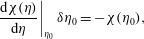


A.2 Global stability analysis
At order
 $\unicode[STIX]{x1D716}^{1}$
the linear eigenvalue problem (3.15) has to be solved and the equations, together with the boundary conditions, are discretized through Chebyshev collocation in a similar fashion to Viola, Arratia & Gallaire (Reference Viola, Arratia and Gallaire2016a
). The physical domain is in general not rectangular due to the presence of the static meniscus
 $\unicode[STIX]{x1D702}_{0}$
. For this reason the physical domain with coordinates
 $(r,z)$
has to be mapped into the Chebyshev space
 $(s,t)$
through the transformation
 $$\begin{eqnarray}r={\displaystyle \frac{R}{2}}(s+1),\quad z=(t+1)\left({\displaystyle \frac{H}{2}}+{\displaystyle \frac{\unicode[STIX]{x1D702}_{0}(s)}{2}}\right)-H,\end{eqnarray}$$
where
 $\unicode[STIX]{x1D702}_{0}$
is the static meniscus. The partial derivatives in the physical space are related to the derivative in the computational space according to the relations
 $$\begin{eqnarray}\left.\begin{array}{@{}c@{}}{\displaystyle \frac{\unicode[STIX]{x2202}u}{\unicode[STIX]{x2202}r}}={\displaystyle \frac{1}{r_{,s}}}u_{,s}-{\displaystyle \frac{z_{,s}}{r_{,s}z_{,t}}}u_{,t}\quad {\displaystyle \frac{\unicode[STIX]{x2202}u}{\unicode[STIX]{x2202}y}}={\displaystyle \frac{1}{z_{,t}}}u_{,t}\\ {\displaystyle \frac{\unicode[STIX]{x2202}^{2}u}{\unicode[STIX]{x2202}r^{2}}}={\displaystyle \frac{1}{r_{,s}^{2}}}u_{,ss}+{\displaystyle \frac{z_{,s}^{2}}{r_{,s}^{2}z_{,t}^{2}}}u_{,tt}-{\displaystyle \frac{z_{,t}z_{,ss}-2z_{,s}z_{,st}}{r_{,s}^{2}z_{,t}^{2}}}u_{,t}-{\displaystyle \frac{2z_{,s}}{r_{,s}^{2}z_{,t}}}u_{,st}\quad {\displaystyle \frac{\unicode[STIX]{x2202}^{2}u}{\unicode[STIX]{x2202}y^{2}}}={\displaystyle \frac{1}{z_{,t}^{2}}}u_{,tt},\end{array}\right\}\end{eqnarray}$$
where the derivatives of the physical coordinates with respect to the computational coordinates depend on the mapping function; see Heinrichs (Reference Heinrichs2004). In our case,
 $$\begin{eqnarray}\left.\begin{array}{@{}c@{}}r_{,s}=R\quad r_{,ss}=0\quad r_{,t}=0\quad r_{,st}=0\quad r_{,tt}=0\\ z_{,s}={\displaystyle \frac{t+1}{2}}\unicode[STIX]{x1D702}_{,s}\quad z_{,ss}={\displaystyle \frac{t+1}{2}}\unicode[STIX]{x1D702}_{,ss}\quad z_{,t}={\displaystyle \frac{H}{2}}+{\displaystyle \frac{\unicode[STIX]{x1D702}(s)}{2}}\quad z_{,st}={\displaystyle \frac{\unicode[STIX]{x1D702}_{,s}}{2}}\quad z_{,tt}=0.\end{array}\right\}\end{eqnarray}$$
The integrals appearing in (3.3) are computed with the Clenshaw–Curtis quadrature formula, where the quadrature weights are adapted to the mappings used following the method presented in Sommariva (Reference Sommariva2013). The number of nodes in the radial and vertical direction is
 $N_{r}=N_{z}=60$
, which ensures convergence of the results. In figure 8(d) the time of arrest as a function of
 $\unicode[STIX]{x1D703}_{s}$
and
 $\unicode[STIX]{x1D6E5}$
computed with the finer grid
 $N_{r}=N_{z}=80$
is reported as proof of convergence.
Appendix B. Adjoint equations
In this section we determine the adjoint equations to the first-order problem (3.15), associated with the Hermitian scalar product:
 $$\begin{eqnarray}\langle \boldsymbol{q}_{\unicode[STIX]{x1D6FC}},\boldsymbol{q}_{\unicode[STIX]{x1D717}}\rangle =\int _{\unicode[STIX]{x1D6FA}}\overline{\unicode[STIX]{x1D6F7}}_{\unicode[STIX]{x1D6FC}}\unicode[STIX]{x1D6F7}_{\unicode[STIX]{x1D717}}\,\text{d}\unicode[STIX]{x1D6FA}+\int _{\unicode[STIX]{x1D702}_{0}}\overline{\unicode[STIX]{x1D702}}_{\unicode[STIX]{x1D6FC}}\unicode[STIX]{x1D702}_{\unicode[STIX]{x1D717}}\,\text{d}\unicode[STIX]{x1D702}_{0},\end{eqnarray}$$
where the overline symbol designates the complex conjugate. The first term is a weighted volume integral with
 $\text{d}\unicode[STIX]{x1D6FA}=r\,\text{d}r\,\text{d}z$
. The second one corresponds to a surface integral on the zero-order surface
 $\unicode[STIX]{x1D702}_{0}(r)$
with
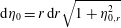 $\text{d}\unicode[STIX]{x1D702}_{0}=r\,\text{d}r\sqrt{1+\unicode[STIX]{x1D702}_{0,r}^{2}}$
. In this section we will demonstrate that the first-order system of equations and boundary conditions are self-adjoint with respect to the scalar product (B 1).
By definition, the adjoint operator of the direct operator
 $\text{i}\unicode[STIX]{x1D714}{\mathcal{B}}-{\mathcal{A}}$
, satisfies
 $$\begin{eqnarray}\langle \boldsymbol{q}^{\dagger },(\text{i}\unicode[STIX]{x1D714}{\mathcal{B}}-{\mathcal{A}})\boldsymbol{q}\rangle =\langle (\text{i}\unicode[STIX]{x1D714}^{\dagger }{\mathcal{B}}^{\dagger }-{\mathcal{A}}^{\dagger })\boldsymbol{q}^{\dagger },\boldsymbol{q}\rangle ,\end{eqnarray}$$
where
 $\boldsymbol{q}^{\dagger }=(\unicode[STIX]{x1D6F7}^{\dagger },\unicode[STIX]{x1D702}^{\dagger })$
is a vector. Hence, the adjoint operator
 $\text{i}\unicode[STIX]{x1D714}^{\dagger }{\mathcal{B}}^{\dagger }-{\mathcal{A}}^{\dagger }$
is derived by integration by parts, transferring the differential operators from the vector
 $\boldsymbol{q}$
to the vector
 $\boldsymbol{q}^{\dagger }$
. The boundary conditions for the adjoint operator are chosen so as to nullify the boundary integrals coming from the integration by parts. The right-hand side of (B 2) reads
 $$\begin{eqnarray}\displaystyle & & \displaystyle \int _{\unicode[STIX]{x1D6FA}}\overline{\unicode[STIX]{x1D6F7}}^{\dagger }\unicode[STIX]{x0394}\unicode[STIX]{x1D6F7}\,\text{d}\unicode[STIX]{x1D6FA}+\int _{\unicode[STIX]{x1D702}_{0}}\overline{\unicode[STIX]{x1D702}}^{\dagger }\left(\text{i}\unicode[STIX]{x1D714}\unicode[STIX]{x1D6F7}+\unicode[STIX]{x1D702}-{\displaystyle \frac{1}{Bo}}\left[{\displaystyle \frac{a(r)}{r}}{\displaystyle \frac{\unicode[STIX]{x2202}\unicode[STIX]{x1D702}}{\unicode[STIX]{x2202}r}}+b(r){\displaystyle \frac{\unicode[STIX]{x2202}^{2}\unicode[STIX]{x1D702}}{\unicode[STIX]{x2202}r^{2}}}-{\displaystyle \frac{m^{2}c(r)}{r^{2}}}\unicode[STIX]{x1D702}\right]\right)\nonumber\\ \displaystyle & & \displaystyle \quad \times \,{\displaystyle \frac{\text{d}\unicode[STIX]{x1D702}_{0}}{\sqrt{1+\unicode[STIX]{x1D702}_{0,r}^{2}}}}=0,\end{eqnarray}$$
where we recall
 $m$
is the azimuthal wavenumber, and integrating by parts we get
 $$\begin{eqnarray}\displaystyle & & \displaystyle \int _{\unicode[STIX]{x1D6FA}}\unicode[STIX]{x0394}\overline{\unicode[STIX]{x1D6F7}}^{\dagger }\unicode[STIX]{x1D6F7}\,\text{d}\unicode[STIX]{x1D6FA}+\int _{\unicode[STIX]{x2202}\unicode[STIX]{x1D6FA}}\overline{\unicode[STIX]{x1D6F7}}^{\dagger }\unicode[STIX]{x1D735}\unicode[STIX]{x1D6F7}\boldsymbol{\cdot }\boldsymbol{n}\,\text{d}S-\int _{\unicode[STIX]{x2202}\unicode[STIX]{x1D6FA}}\unicode[STIX]{x1D6F7}\unicode[STIX]{x1D735}\overline{\unicode[STIX]{x1D6F7}}^{\dagger }\boldsymbol{\cdot }\boldsymbol{n}\,\text{d}S\nonumber\\ \displaystyle & & \displaystyle \quad +\,\int _{\unicode[STIX]{x1D702}_{0}}-\overline{\text{i}\unicode[STIX]{x1D714}\unicode[STIX]{x1D702}^{\dagger }}\unicode[STIX]{x1D6F7}r\,\text{d}r+\int _{\unicode[STIX]{x1D702}_{0}}\left(\overline{\unicode[STIX]{x1D702}}^{\dagger }-{\displaystyle \frac{1}{Bo}}\left[{\displaystyle \frac{a(r)}{r}}{\displaystyle \frac{\unicode[STIX]{x2202}\overline{\unicode[STIX]{x1D702}}^{\dagger }}{\unicode[STIX]{x2202}r}}+b(r){\displaystyle \frac{\unicode[STIX]{x2202}^{2}\overline{\unicode[STIX]{x1D702}}^{\dagger }}{\unicode[STIX]{x2202}r^{2}}}-{\displaystyle \frac{m^{2}c(r)}{r^{2}}}\overline{\unicode[STIX]{x1D702}}^{\dagger }\right]\right)\unicode[STIX]{x1D702}r\,\text{d}r\nonumber\\ \displaystyle & & \displaystyle \quad -\,{\displaystyle \frac{1}{Bo}}\left[rb(r)\left(\overline{\unicode[STIX]{x1D702}}^{\dagger }{\displaystyle \frac{\unicode[STIX]{x2202}\unicode[STIX]{x1D702}}{\unicode[STIX]{x2202}r}}-{\displaystyle \frac{\unicode[STIX]{x2202}\overline{\unicode[STIX]{x1D702}}^{\dagger }}{\unicode[STIX]{x2202}r}}\unicode[STIX]{x1D702}\right)\right]_{r=0}^{r=1}=0.\end{eqnarray}$$
The first integral comes from the integration of the continuity equation, and it is nullified by imposing that the adjoint potential
 $\unicode[STIX]{x0394}\unicode[STIX]{x1D6F7}^{\dagger }=0$
is harmonic. The integrals on the domain boundary
 $\unicode[STIX]{x2202}\unicode[STIX]{x1D6FA}$
involving the normal velocity
 $\unicode[STIX]{x1D735}\unicode[STIX]{x1D6F7}\boldsymbol{\cdot }\boldsymbol{n}$
are the boundary terms resulting in the integration by parts of the continuity equation. These terms vanish at the solid wall because of the no-penetration condition
 $$\begin{eqnarray}\displaystyle \left.{\displaystyle \frac{\unicode[STIX]{x2202}\unicode[STIX]{x1D6F7}}{\unicode[STIX]{x2202}r}}\right|_{r=1}=\left.{\displaystyle \frac{\unicode[STIX]{x2202}\unicode[STIX]{x1D6F7}}{\unicode[STIX]{x2202}z}}\right|_{z=-h}=\left.{\displaystyle \frac{\unicode[STIX]{x2202}\unicode[STIX]{x1D6F7}^{\dagger }}{\unicode[STIX]{x2202}r}}\right|_{r=1}=\left.{\displaystyle \frac{\unicode[STIX]{x2202}\unicode[STIX]{x1D6F7}^{\dagger }}{\unicode[STIX]{x2202}z}}\right|_{z=-h}=0, & & \displaystyle\end{eqnarray}$$
and at the axis because of the symmetry condition
 $$\begin{eqnarray}\unicode[STIX]{x1D6F7}|_{r=0}=\unicode[STIX]{x1D6F7}^{\dagger }|_{r=0}=0.\end{eqnarray}$$
At the free interface the domain is curved, and the normal vector is
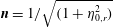 $\boldsymbol{n}=1/\sqrt{(1+\unicode[STIX]{x1D702}_{0,r}^{2})}$
 $(\begin{smallmatrix}-\unicode[STIX]{x1D702}_{0,r}\\ 1\end{smallmatrix})$
. By using the kinematic boundary conditions (3.10), equation (B 4) reads
 $$\begin{eqnarray}\displaystyle & & \displaystyle \int _{\unicode[STIX]{x1D702}_{0}}\left(-\overline{\text{i}\unicode[STIX]{x1D714}\unicode[STIX]{x1D702}^{\dagger }}+\unicode[STIX]{x1D702}_{0,r}{\displaystyle \frac{\unicode[STIX]{x2202}\overline{\unicode[STIX]{x1D6F7}}^{\dagger }}{\unicode[STIX]{x2202}r}}-{\displaystyle \frac{\unicode[STIX]{x2202}\overline{\unicode[STIX]{x1D6F7}}^{\dagger }}{\unicode[STIX]{x2202}z}}\right)\unicode[STIX]{x1D6F7}{\displaystyle \frac{\text{d}\unicode[STIX]{x1D702}_{0}}{\sqrt{1+\unicode[STIX]{x1D702}_{0,r^{2}}}}}\nonumber\\ \displaystyle & & \displaystyle \quad +\,\int _{\unicode[STIX]{x1D702}_{0}}\left(-\overline{\text{i}\unicode[STIX]{x1D714}\unicode[STIX]{x1D6F7}^{\dagger }}+\overline{\unicode[STIX]{x1D702}}^{\dagger }-{\displaystyle \frac{1}{Bo}}\left[{\displaystyle \frac{a(r)}{r}}{\displaystyle \frac{\unicode[STIX]{x2202}\overline{\unicode[STIX]{x1D702}}^{\dagger }}{\unicode[STIX]{x2202}r}}+b(r){\displaystyle \frac{\unicode[STIX]{x2202}^{2}\overline{\unicode[STIX]{x1D702}}^{\dagger }}{\unicode[STIX]{x2202}r^{2}}}-{\displaystyle \frac{m^{2}c(r)}{r^{2}}}\unicode[STIX]{x1D702}^{\dagger }\right]\right)\unicode[STIX]{x1D702}{\displaystyle \frac{\text{d}\unicode[STIX]{x1D702}_{0}}{\sqrt{1+\unicode[STIX]{x1D702}_{0,r^{2}}}}}\nonumber\\ \displaystyle & & \displaystyle \quad -\,{\displaystyle \frac{1}{Bo}}\left[rb(r)\left(\overline{\unicode[STIX]{x1D702}}^{\dagger }{\displaystyle \frac{\unicode[STIX]{x2202}\unicode[STIX]{x1D702}}{\unicode[STIX]{x2202}r}}-{\displaystyle \frac{\unicode[STIX]{x2202}\overline{\unicode[STIX]{x1D702}}^{\dagger }}{\unicode[STIX]{x2202}r}}\unicode[STIX]{x1D702}\right)\right]_{r=0}^{r=1}=0.\end{eqnarray}$$
From the first two terms in (B 7) the adjoint kinematic and dynamic interface conditions are retrieved:
 $$\begin{eqnarray}\left.\begin{array}{@{}c@{}}-\text{i}\unicode[STIX]{x1D714}\unicode[STIX]{x1D702}^{\dagger }+\unicode[STIX]{x1D702}_{0,r}{\displaystyle \frac{\unicode[STIX]{x2202}\unicode[STIX]{x1D6F7}^{\dagger }}{\unicode[STIX]{x2202}r}}-{\displaystyle \frac{\unicode[STIX]{x2202}\unicode[STIX]{x1D6F7}^{\dagger }}{\unicode[STIX]{x2202}z}}=0,\\ -\text{i}\unicode[STIX]{x1D714}\unicode[STIX]{x1D6F7}^{\dagger }+\unicode[STIX]{x1D702}^{\dagger }-{\displaystyle \frac{1}{Bo}}\left[{\displaystyle \frac{a(r)}{r}}{\displaystyle \frac{\unicode[STIX]{x2202}\unicode[STIX]{x1D702}^{\dagger }}{\unicode[STIX]{x2202}r}}+b(r){\displaystyle \frac{\unicode[STIX]{x2202}^{2}\unicode[STIX]{x1D702}^{\dagger }}{\unicode[STIX]{x2202}r^{2}}}-{\displaystyle \frac{m^{2}c(r)}{r^{2}}}\unicode[STIX]{x1D702}^{\dagger }\right]=0.\end{array}\right\}\end{eqnarray}$$
To complete the adjoint system of equations the last term in (B 7), which comes from the integration by parts of the capillary pressure in the direct dynamic condition, has to be nullified. In
 $r=0$
this term is null because of the integral argument is weighted by
 $r$
. In contrast, at the contact line
 $b(r=1)=\sin ^{3}(\unicode[STIX]{x1D703}_{s})$
and the condition
 $$\begin{eqnarray}-{\displaystyle \frac{\sin ^{3}(\unicode[STIX]{x1D703}_{s})}{Bo}}\left.\left(\overline{\unicode[STIX]{x1D702}}^{\dagger }{\displaystyle \frac{\unicode[STIX]{x2202}\unicode[STIX]{x1D702}}{\unicode[STIX]{x2202}r}}-{\displaystyle \frac{\unicode[STIX]{x2202}\overline{\unicode[STIX]{x1D702}}^{\dagger }}{\unicode[STIX]{x2202}r}}\unicode[STIX]{x1D702}\right)\right|_{r=1}=0\end{eqnarray}$$
defines the natural boundary condition at the contact line. In the case of free-end edge interface,
 $$\begin{eqnarray}\left.{\displaystyle \frac{\unicode[STIX]{x2202}\unicode[STIX]{x1D702}}{\unicode[STIX]{x2202}r}}\right|_{r=1}=\left.{\displaystyle \frac{\unicode[STIX]{x2202}\unicode[STIX]{x1D702}^{\dagger }}{\unicode[STIX]{x2202}r}}\right|_{r=1}=0.\end{eqnarray}$$
It should be noted that also the pinned boundary condition
 $\unicode[STIX]{x1D702}=\unicode[STIX]{x1D702}^{\dagger }=0$
is a natural boundary condition of the problem. Hence the direct problem at order
 $\unicode[STIX]{x1D716}$
is self-adjoint with respect to the Hermitian scalar product (B 1):
 $$\begin{eqnarray}\text{i}\unicode[STIX]{x1D714}^{\dagger }{\mathcal{B}}^{\dagger }-{\mathcal{A}}^{\dagger }=-\text{i}\unicode[STIX]{x1D714}{\mathcal{B}}-{\mathcal{A}},\end{eqnarray}$$
with
 $\unicode[STIX]{x1D714}^{\dagger }=-\unicode[STIX]{x1D714}$
. The vector
 $\boldsymbol{q}^{\dagger }$
which satisfies the adjoint equations
 $[-\text{i}\unicode[STIX]{x1D714}{\mathcal{B}}-{\mathcal{A}}]\boldsymbol{q}^{\dagger }=0$
is the adjoint mode.
Appendix C. Asymptotic analysis validation: comparison with direct numerical simulation
In this section the validity of the weakly nonlinear analysis is discussed through a comparison with a direct numerical simulation of the governing equations presented in § 2, in the limit of small oscillations. The continuity equation
 $$\begin{eqnarray}\unicode[STIX]{x0394}\unicode[STIX]{x1D6F7}=0,\end{eqnarray}$$
is completed by the dynamic and kinematic conditions at the free surface that in the case of static contact angle
 $\unicode[STIX]{x1D703}_{s}=\unicode[STIX]{x03C0}/2$
read
 $$\begin{eqnarray}\left.\begin{array}{@{}c@{}}{\displaystyle \frac{\unicode[STIX]{x2202}\unicode[STIX]{x1D6F7}}{\unicode[STIX]{x2202}t}}+\unicode[STIX]{x1D702}-{\displaystyle \frac{1}{Bo}}\unicode[STIX]{x1D702}=0\quad \text{ at }z=0,\\ {\displaystyle \frac{\unicode[STIX]{x2202}\unicode[STIX]{x1D702}}{\unicode[STIX]{x2202}t}}=\left.{\displaystyle \frac{\unicode[STIX]{x2202}\unicode[STIX]{x1D6F7}}{\unicode[STIX]{x2202}z}}\right|_{0}\quad \text{ at }z=0.\end{array}\right\}\end{eqnarray}$$
Symmetry conditions at the axis and the no-penetration condition at the solid walls also need to be satisfied. The nonlinear wetting condition is then imposed at the contact line:
 $$\begin{eqnarray}\left.-{\displaystyle \frac{\unicode[STIX]{x2202}\unicode[STIX]{x1D702}}{\unicode[STIX]{x2202}r}}\right|_{r=1}=\unicode[STIX]{x1D6FC}Ca\left.{\displaystyle \frac{\unicode[STIX]{x2202}\unicode[STIX]{x1D702}}{\unicode[STIX]{x2202}t}}\right|_{r=1}+{\displaystyle \frac{\unicode[STIX]{x1D6E5}}{2}}\tanh \left(\unicode[STIX]{x1D6FD}Ca\left.{\displaystyle \frac{\unicode[STIX]{x2202}\unicode[STIX]{x1D702}}{\unicode[STIX]{x2202}t}}\right|_{r=1}\right)\quad \text{at }z=0\text{ and }r=1.\end{eqnarray}$$
In order to investigate the dynamics of the fundamental sloshing mode (first azimuthal mode) the state vector
 $\boldsymbol{q}(t;r,\unicode[STIX]{x1D719},z)=(\unicode[STIX]{x1D6F7},\unicode[STIX]{x1D702})$
can be written as a truncated Fourier series,
 $$\begin{eqnarray}\hat{\boldsymbol{q}}(t;r,\unicode[STIX]{x1D719},z)=\hat{\boldsymbol{q}}_{1}(t;r,z)\text{e}^{\text{i}\unicode[STIX]{x1D719}}+\text{c.c.},\end{eqnarray}$$
where
 $\text{c.c.}$
stands for complex conjugate. By injecting the modal expansion (C 4) in the nonlinear equation (C 3) we get
 $$\begin{eqnarray}\left.-{\displaystyle \frac{\unicode[STIX]{x2202}\hat{\unicode[STIX]{x1D702}}_{1}}{\unicode[STIX]{x2202}r}}\right|_{r=1}\text{e}^{\text{i}\unicode[STIX]{x1D719}}+\text{c.c.}=\unicode[STIX]{x1D6FC}Ca\left(\left.{\displaystyle \frac{\unicode[STIX]{x2202}\hat{\unicode[STIX]{x1D702}}_{1}}{\unicode[STIX]{x2202}t}}\right|_{r=1}\text{e}^{\text{i}\unicode[STIX]{x1D719}}+\text{c.c.}\right)+{\displaystyle \frac{\unicode[STIX]{x1D6E5}}{2}}\underbrace{\tanh \left(\unicode[STIX]{x1D6FD}Ca\left(\left.{\displaystyle \frac{\unicode[STIX]{x2202}\hat{\unicode[STIX]{x1D702}}_{1}}{\unicode[STIX]{x2202}t}}\right|_{r=1}\text{e}^{\text{i}\unicode[STIX]{x1D719}}+\text{c.c.}\right)\right)\sum }_{\mathop{\sum }_{n}F_{n}\text{e}^{\text{i}m\unicode[STIX]{x1D719}}},\end{eqnarray}$$
where the last term on the right-hand side has to be Fourier transformed to get a boundary condition for the fundamental mode
 $$\begin{eqnarray}\left.{\displaystyle \frac{\unicode[STIX]{x2202}\hat{\unicode[STIX]{x1D702}}_{1}}{\unicode[STIX]{x2202}r}}\right|_{r=1}\text{e}^{\text{i}\unicode[STIX]{x1D719}}+\text{c.c.}=-\unicode[STIX]{x1D6FC}Ca\left.{\displaystyle \frac{\unicode[STIX]{x2202}\hat{\unicode[STIX]{x1D702}}_{1}}{\unicode[STIX]{x2202}t}}\right|_{r=1}\text{e}^{\text{i}\unicode[STIX]{x1D719}}-{\displaystyle \frac{\unicode[STIX]{x1D6E5}}{2}}F_{1}(\unicode[STIX]{x1D6FD},Ca,t)\text{e}^{\text{i}\unicode[STIX]{x1D719}}+\text{c.c.},\end{eqnarray}$$
with
 $$\begin{eqnarray}F_{1}(\unicode[STIX]{x1D6FD},Ca,t)={\displaystyle \frac{1}{2\unicode[STIX]{x03C0}}}\int _{0}^{2\unicode[STIX]{x03C0}}\tanh \left(\unicode[STIX]{x1D6FD}Ca\left(\left.{\displaystyle \frac{\unicode[STIX]{x2202}\hat{\unicode[STIX]{x1D702}}_{1}}{\unicode[STIX]{x2202}t}}\right|_{r=1}\text{e}^{\text{i}\unicode[STIX]{x1D719}}+\text{c.c.}\right)\right)\text{e}^{-\text{i}\unicode[STIX]{x1D719}}\,\text{d}\unicode[STIX]{x1D719}.\end{eqnarray}$$
(a) Contact line model for
 $\unicode[STIX]{x1D6E5}=5^{\circ }$
,
 $\unicode[STIX]{x1D6FC}=1$
,
 $Bo=500$
,
 $Ca=0.01$
and
 $\unicode[STIX]{x1D703}_{s}=\unicode[STIX]{x03C0}/2$
. The steepness coefficient is varied as
 $\unicode[STIX]{x1D6FD}=100$
, 1000 and 10 000. The contact line motion according to the weakly nonlinear analysis (blue line, its amplitude is depicted by a red line) and the solution from numerics (circles) are shown for (c)
 $\unicode[STIX]{x1D6FD}=100$
, (d)
 $\unicode[STIX]{x1D6FD}=1000$
and (e)
 $\unicode[STIX]{x1D6FD}=10\,000$
. The corresponding damping rates are reported in (b).
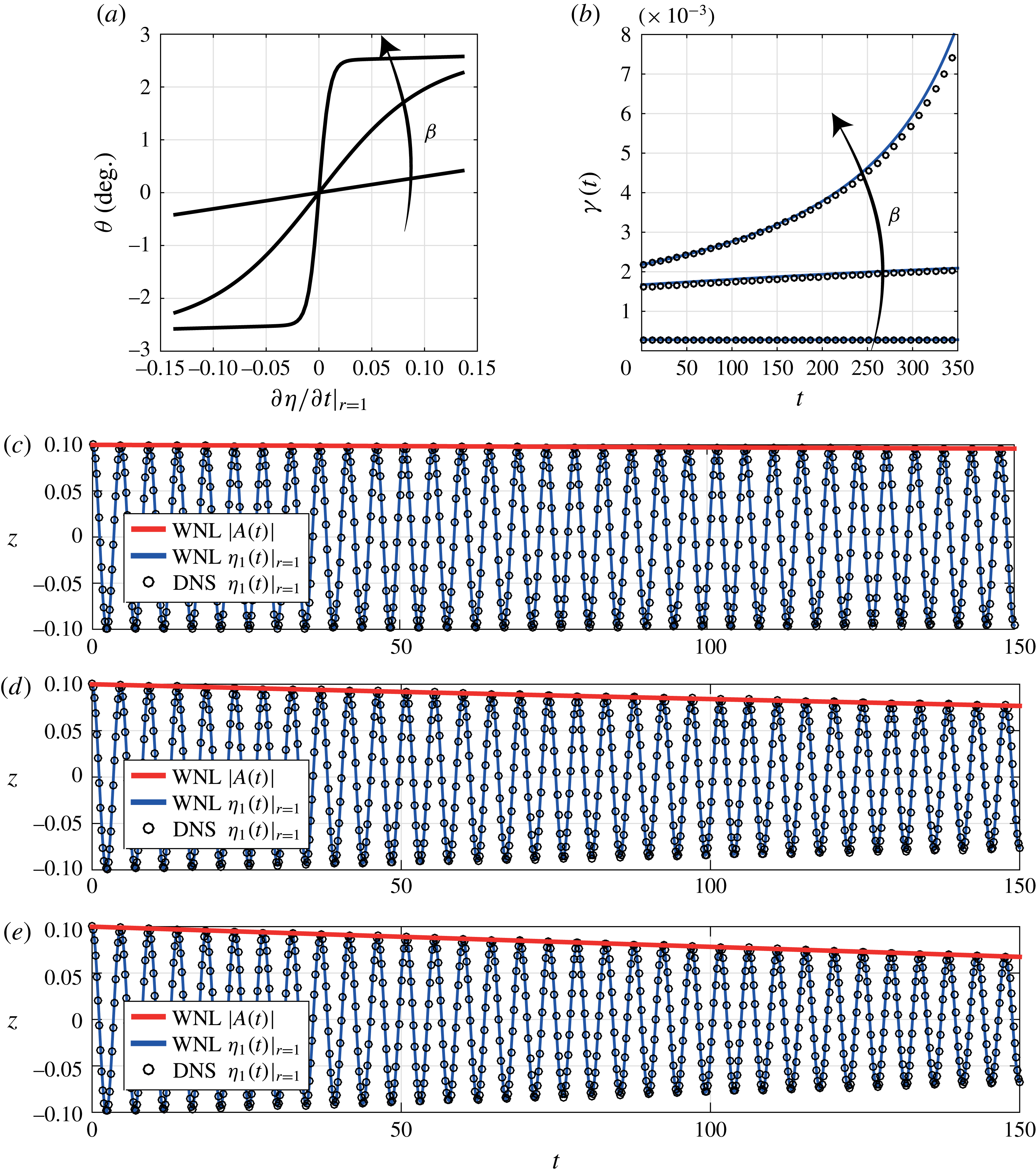
(a) Contact line model for
 $\unicode[STIX]{x1D6FD}=1000$
,
 $\unicode[STIX]{x1D6FC}=1$
,
 $Bo=500$
,
 $Ca=0.01$
and
 $\unicode[STIX]{x1D703}_{s}=\unicode[STIX]{x03C0}/2$
. The contact angle hysteresis is varied as
 $\unicode[STIX]{x1D6E5}=5^{\circ },10^{\circ }$
and
 $20^{\circ }$
. The contact line motion according to the weakly nonlinear analysis (blue line, its amplitude is depicted by a red line) and the solution from numerics (circles) are shown for (c)
 $\unicode[STIX]{x1D6E5}=5^{\circ }$
, (d)
 $\unicode[STIX]{x1D6E5}=10^{\circ }$
and (e)
 $\unicode[STIX]{x1D6E5}=20^{\circ }$
. The corresponding damping rates are reported in (b).

The resulting equations for
 $\hat{\boldsymbol{q}}_{1}(t;r,z)$
are then discretized in space by means of a pseudospectral Chebyshev–Chebyshev method as introduced in § 3.2 and appendix A. A backward differentiation formula of second order is employed for time integration. This integration scheme is implicit and especially suited for solving stiff differential equations like our case where the continuity of mass (C 1) is an algebraic constraint for the unsteady kinematic and boundary conditions (C 2). The discretized state vector
 $\boldsymbol{q}^{n}$
after
 $n$
time steps of size
 $\unicode[STIX]{x1D6FF}t$
is obtained by solving
 $$\begin{eqnarray}{\textstyle \frac{3}{2}}{\mathcal{B}}\boldsymbol{q}^{n}-2{\mathcal{B}}\boldsymbol{q}^{n-1}+{\textstyle \frac{1}{2}}{\mathcal{B}}\boldsymbol{q}^{n-2}=\unicode[STIX]{x1D6FF}t({\mathcal{A}}\boldsymbol{q}^{n}+\boldsymbol{f}(v_{c}))\end{eqnarray}$$
where
 ${\mathcal{A}}$
and
 ${\mathcal{B}}$
contain the discretized equations; see (3.13). The vector
 $\boldsymbol{f}(v_{c})$
is nil everywhere except for its component corresponding to the contact line (
 $z=0$
and
 $r=1$
), which is equal to the last term of (C 6). The remaining term on the right-hand side of (C 6) is contained in
 ${\mathcal{B}}$
while the left-hand side of (C 6) is discretized in
 ${\mathcal{A}}$
. The quantity
 $v_{c}$
is the contact line velocity
 $v_{c}=(\unicode[STIX]{x2202}\unicode[STIX]{x1D702}/\unicode[STIX]{x2202}t)|_{r=1}$
that can be treated explicitly or implicitly respectively. With an explicit scheme using the interface position at previous times,
 $v_{c}$
reads
 $$\begin{eqnarray}v_{c}=v_{c}^{n-1}={\displaystyle \frac{\unicode[STIX]{x1D702}_{n-1}+4/3\unicode[STIX]{x1D702}_{n-2}+1/3\unicode[STIX]{x1D702}_{n-3}}{2/3\unicode[STIX]{x1D6FF}t}}\end{eqnarray}$$
and can be readily used to compute
 $\boldsymbol{q}^{n}$
. In contrast, if an implicit formula is used, the velocity
 $$\begin{eqnarray}v_{c}=v_{c}^{n}={\displaystyle \frac{\unicode[STIX]{x1D702}_{n}+4/3\unicode[STIX]{x1D702}_{n-1}+1/3\unicode[STIX]{x1D702}_{n-2}}{2/3\unicode[STIX]{x1D6FF}t}}\end{eqnarray}$$
depends on the unknown interface position
 $\unicode[STIX]{x1D702}_{n}$
and an iterative procedure is needed due to the nonlinear relation
 $\boldsymbol{f}(v_{c})$
. In this case, in order to advance from the time
 $t^{n-1}$
towards the next one
 $t^{n}=t^{n-1}+\unicode[STIX]{x1D6FF}t$
, a guess contact line velocity
 $v_{c}^{n\ast }$
is chosen (typically the one at previous time step
 $v_{c}^{n-1}$
) which is then used to compute
 $\boldsymbol{q}^{n\ast \ast }$
through (C 8). If the difference between the updated contact line velocity
 $v_{c}^{n\ast \ast }$
and the guess velocity is larger than a given threshold, the guess velocity is conveniently modified and the procedure repeated. This method has been implemented by using fsolve, a built-in Matlab function designed to solve nonlinear equations, which has been employed here to determine the contact line velocity
 $v_{c}^{n}$
at every time step. The two methods provide similar results. The implicit treatment of the contact line velocity allows for larger time step, typically
 $\unicode[STIX]{x1D6FF}t=0.05$
rather than
 $\unicode[STIX]{x1D6FF}t=0.01$
used in explicit case, but the subiterative procedure slows down computation speed.
Let us now compare the dynamics of the fundamental sloshing mode resulting from the numerical simulation with that coming from the weakly nonlinear analysis introduced in the main body of the paper. In figure 11 the contact line hysteresis is set to
 $\unicode[STIX]{x1D6E5}=5^{\circ }$
whereas the steepness coefficient is varied as
 $\unicode[STIX]{x1D6FD}=100$
, 1000 and 10 000: see figure 11(a). The corresponding contact line motion is reported in figure 11(c,d,e) where the asymptotic solution (blue line) and its instantaneous amplitude (red line) match well the numerical results (circles) for all the values of
 $\unicode[STIX]{x1D6FD}$
. Furthermore, a satisfactory agreement on the damping rate,
 $\unicode[STIX]{x1D6FE}(t)$
, is also observed: see figure 11(b). In particular, for
 $\unicode[STIX]{x1D6FD}=100$
the damping rate is practically uniform and increases almost linearly for
 $\unicode[STIX]{x1D6FD}=1000$
. In the case of higher steepness factor
 $\unicode[STIX]{x1D6FD}=10\,000$
,
 $\unicode[STIX]{x1D6FE}(t)$
increases significantly, getting three times the initial value at
 $t=350$
.
In figure 12 the steepness coefficient is fixed to
 $\unicode[STIX]{x1D6FD}=1000$
and the contact angle hysteresis is progressively increased as
 $\unicode[STIX]{x1D6E5}=5^{\circ }$
,
 $10^{\circ }$
and
 $20^{\circ }$
. The other parameters are set as in the previous case: see captions. The resulting contact line laws are shown in figure 12(a): the contact angle depends nonlinearly on the contact line velocity and the more
 $\unicode[STIX]{x1D6E5}$
increases, the more
 $\unicode[STIX]{x1D703}$
varies. The resulting contact line motions as a function of time are shown in figure 12(c,d,e) pointing to good agreement between asymptotics and numerics. The damping rates are then shown in figure 12(e) thus revealing a stronger nonlinear behaviour for higher contact line hysteresis
 $\unicode[STIX]{x1D6E5}$
that is captured both from the asymptotic analysis and numerics.
Despite the good agreement between asymptotic analysis and numeric simulations, the steepness coefficient
 $\unicode[STIX]{x1D6FD}$
and the hysteresis parameter
 $\unicode[STIX]{x1D6E5}$
could not be further increased in the numerical simulations with respect to the values reported here. This is due to the stiffness of the governing equations and the strong nonlinearity of the adopted contact line law which arguably require more sophisticated time schemes to integrate the solution in the case of a steeper and more intense contact angle hysteresis.