1 Introduction
The understanding of the dynamics of turbulence has been recently boosted by the adoption of a dynamical-system representation of the problem, inspired by the early work of Hopf (Reference Hopf1948) and extended during the last 20 years to the case of turbulent shear flows. According to this dynamical view point, the time evolution of the flow corresponds to a trajectory in state space, which recurrently approaches the exact invariant solutions populating the state space. Turbulence is linked to the existence of a multitude of such invariant solutions of the Navier–Stokes (NS) equations (Budanur et al.
Reference Budanur, Short, Farazmand, Willis and Cvitanović2017), in the form of equilibria, travelling waves, periodic orbits and relative periodic orbits (Kawahara, Uhlmann & Van Veen Reference Kawahara, Uhlmann and Van Veen2012). The transiently visited solutions capture organized flow structures, such as streaks in turbulent boundary layers, as well as puffs in pipe flows (Hof et al.
Reference Hof, van Doorne, Westerweel, Nieuwstadt, Faisst, Eckhardt, Wedin, Kerswell and Waleffe2004), and are thus also termed exact coherent states (ECSs). Due to their dynamical relevance there has been a strong recent effort to compute invariant solutions, especially for pipe (Faisst & Eckhardt Reference Faisst and Eckhardt2003; Wedin & Kerswell Reference Wedin and Kerswell2004; Duguet, Willis & Kerswell Reference Duguet, Willis and Kerswell2008; Willis, Cvitanović & Avila Reference Willis, Cvitanović and Avila2013; Budanur et al.
Reference Budanur, Short, Farazmand, Willis and Cvitanović2017) and Couette flow (Nagata Reference Nagata1990; Kawahara & Kida Reference Kawahara and Kida2001; Viswanath Reference Viswanath2007; Gibson, Halcrow & Cvitanović Reference Gibson, Halcrow and Cvitanović2008; Schneider et al.
Reference Schneider, Gibson, Lagha, De Lillo and Eckhardt2008; Gibson, Halcrow & Cvitanović Reference Gibson, Halcrow and Cvitanović2009; Halcrow et al.
Reference Halcrow, Gibson, Cvitanović and Viswanath2009). In these two reference flow cases, the state space contains a linearly stable equilibrium solution corresponding to the laminar flow state, as well as a chaotic set supporting turbulent dynamics. Embedded in the chaotic saddle are ECSs dynamically connected by their entangled stable and unstable manifolds. The ECSs are all unstable so that a turbulent trajectory is believed to be transiently attracted to an individual ECS along its stable manifold before it leaves along the unstable manifold and is captured by another ECS. Within the emerging dynamical systems picture, turbulence can thus be understood as a walk along dynamical connections between various ECSs (Suri et al.
Reference Suri, Tithof, Grigoriev and Schatz2017). To characterize the turbulence-supporting saddle we not only need to compute the invariant states but also identify homo- and heteroclinic connections between them. These connections form the network along which turbulent trajectories evolve between the ECSs and are thus key for understanding the turbulent dynamics. Unfortunately, finding heteroclinic connections is a very difficult task and there is no general and robust algorithm to compute them. In fact, the first heteroclinic connection between two equilibria of the three-dimensional (3D) Navier–Stokes equations for a shear flow has been reported only recently. Gibson et al. (Reference Gibson, Halcrow and Cvitanović2008) identified a connection in Couette flow at Reynolds number
 $Re=400$
. For the same flow and parameters, two additional heteroclinic connections have been reported by the same research group (Halcrow et al.
Reference Halcrow, Gibson, Cvitanović and Viswanath2009). A homoclinic connection from and to the edge state in plane Couette flow was identified by Van Veen & Kawahara (Reference Van Veen and Kawahara2011), who showed that this connection underlies strongly dissipative bursting events. Evidence for a likely heteroclinic connection between two relative periodic orbits for the case of pipe flow has been recently found by Hof & Budanur (Reference Hof and Budanur2017). A periodic-like solution (Toh & Itano Reference Toh and Itano2003) in plane Poiseuille flow suggests heteroclinic connection between a single-streak and a double-streak state. Likewise a connection between two symmetry-related travelling waves on the laminar-turbulent boundary for the asymptotic suction boundary layer is strongly suggested by Kreilos et al. (Reference Kreilos, Veble, Schneider and Eckhardt2013). These studies suggest that connections between exact invariant solutions are dynamically relevant and may underlie both bursts and puff formation. Despite their obvious importance, for full 3D shear flows the only currently available algorithms for computing heteroclinic connections are the shooting method of Halcrow et al. (Reference Halcrow, Gibson, Cvitanović and Viswanath2009) and the boundary-value problem approach by Van Veen, Kawahara & Atsushi (Reference Van Veen, Kawahara and Atsushi2011).
We propose an alternative method for identifying heteroclinic connections and apply it to plane Couette flow at
 $Re=400$
. The method entails two steps. First, we construct an orbit that connects small energy shells around two equilibrium states. This step is based on nonlinear minimization using the Lagrange multiplier method. In a second step, we use local information on the dynamics linearized around the initial and final equilibria to confirm that the constructed orbit shadows a heteroclinic connection located within the intersection of the unstable manifold of the initial and the stable manifold of the final equilibria. We first present the numerical approach and validate the method with respect to the results of Halcrow et al. (Reference Halcrow, Gibson, Cvitanović and Viswanath2009), obtaining the same three heteroclinic connections. Then, the proposed method is used to identify six new heteroclinic connections. Finally, we discuss advantages and limitations of the proposed method in comparison to alternative approaches for computing heteroclinic connections.
2 Problem formulation
We consider plane Couette flow at Reynolds number
 $Re=400$
, where non-dimensional variables are chosen to have half of the distance between the plates equal to
 $h=1$
and half of the difference between the velocity of the two plates equal to
 $1$
. The problem is studied by numerically solving the Navier–Stokes equations for incompressible flow. Simulations are performed in a computational domain of streamwise and spanwise size
 $L_{x}=2\unicode[STIX]{x03C0}/1.14$
and
 $L_{z}=2\unicode[STIX]{x03C0}/2.5$
, respectively (Waleffe Reference Waleffe2003).
 $x$
,
 $y$
,
 $z$
represent the streamwise, wall-normal and spanwise coordinates, and
 $u$
,
 $v$
,
 $w$
are the three corresponding Cartesian components of the velocity vector,
 $\boldsymbol{u}$
. Dirichlet boundary conditions for the three velocity components are imposed at the upper and lower wall (
 $u_{wall}=\pm 1$
), whereas periodicity is prescribed in the streamwise and spanwise directions. Computations are performed using Channelflow (Gibson Reference Gibson2014). For spectral discretization, we use 32 Fourier points in the
 $x$
and
 $z$
directions and 35 Chebyshev points in the
 $y$
direction. Both domain and discretization are identical to Halcrow et al. (Reference Halcrow, Gibson, Cvitanović and Viswanath2009) in order to validate our procedure with their results.
3 Algorithm for computing heteroclinic connections
The main idea of the present work is to employ a nonlinear variational minimization algorithm based on an iterative direct-adjoint procedure (Cherubini et al. Reference Cherubini, De Palma, Robinet and Bottaro2010; Pringle & Kerswell Reference Pringle and Kerswell2010; Kerswell Reference Kerswell2018) to compute connections between finite neighbourhoods of equilibrium states and show that those orbits approximate heteroclinic connections. Alternative variational approaches have also been proposed for computing periodic orbits (Lan & Cvitanović Reference Lan and Cvitanović2004) and heteroclinic connections in lower-dimensional problems (Dong & Lan Reference Dong and Lan2014) including two-dimensional (2D) atmospheric flow models (Crommelin Reference Crommelin2003).
Along a heteroclinic connection, the trajectory leaves the initial equilibrium (
 $EQ_{out}$
) to approach the final equilibrium (
 $EQ_{in}$
). Since it takes an infinite time to traverse the connection we approximate it by a trajectory starting in a small but finite neighbourhood of the initial equilibrium and reaching the neighbourhood of the final one. The passage time
 $T$
is finite and we ensure that results are robust with respect to the choice of the neighbourhoods.
Technically, we fix energy shells
 $E_{0_{out}}$
and
 $E_{0_{in}}$
, around the initial and final equilibrium. For fixed passage time
 $T$
we find the initial perturbation
 $\boldsymbol{u}^{\prime }(0)=\boldsymbol{u}(0)-\boldsymbol{u}_{EQ_{out}}$
constrained to
 $E_{0_{out}}$
, such that the distance from the final equilibrium is minimized at passage time
 $T$
. By gradually increasing the passage time, we determine the time
 $T$
of the first local minimum of the objective function lower than a chosen threshold
 $E_{0_{in}}$
.
For minimizing the distance from the final equilibrium
 $E(T)=\Vert \boldsymbol{u}^{\prime }(T)+\boldsymbol{u}_{EQ_{out}}-\boldsymbol{u}_{EQ_{in}}\Vert _{2}^{2}$
, with
 $\Vert \bullet \Vert _{2}^{2}=1/V\int _{V}\bullet ^{2}\,\text{d}V$
, and
 $V$
the volume of the computational domain, we consider the Lagrangian
 $$\begin{eqnarray}\displaystyle & & \displaystyle {\mathcal{L}}(\boldsymbol{u}^{\prime },p^{\prime },\boldsymbol{u}^{\dagger },p^{\dagger },\boldsymbol{u}^{\prime }(T),\boldsymbol{u}^{\prime }(0),\unicode[STIX]{x1D706})=\Vert \boldsymbol{u}^{\prime }(T)+\boldsymbol{u}_{EQ_{out}}-\boldsymbol{u}_{EQ_{in}}\Vert _{2}^{2}\nonumber\\ \displaystyle & & \displaystyle \qquad -\,\int _{0}^{T}\langle \boldsymbol{u}^{\dagger },NS(\boldsymbol{u}^{\prime },\boldsymbol{u}_{EQ_{out}},p^{\prime })\rangle \,\text{d}t-\int _{0}^{T}\langle p^{\dagger },\unicode[STIX]{x1D735}\boldsymbol{\cdot }\boldsymbol{u}^{\prime }\rangle \,\text{d}t-\unicode[STIX]{x1D706}(\Vert \boldsymbol{u}^{\prime }(0)\Vert _{2}^{2}-E_{0_{out}}),\nonumber\\ \displaystyle & & \displaystyle\end{eqnarray}$$
where
 $\langle \boldsymbol{a},\boldsymbol{b}\rangle$
indicates the scalar product
 $1/V\int _{V}(\boldsymbol{a}\boldsymbol{\cdot }\boldsymbol{b})\,\text{d}V$
. Setting the variation of
 ${\mathcal{L}}$
with respect to the fields
 $\boldsymbol{u}^{\prime },p^{\prime }$
to zero yields adjoint equations for the Lagrange multipliers
 $\boldsymbol{u}^{\dagger },p^{\dagger }$
that enforce the NS equations. The vanishing gradient with respect to
 $\boldsymbol{u}^{\prime }(T)$
yields the compatibility conditions at
 $t=T$
, namely,
 $\boldsymbol{u}^{\dagger }(T)=\boldsymbol{u}^{\prime }(T)+\boldsymbol{u}_{EQ_{out}}-\boldsymbol{u}_{EQ_{in}}$
. Integrating the NS equations from
 $t=0$
to
 $t=T$
, using the compatibility condition to initialize the adjoint equations and integrating them backwards in time from
 $t=T$
to
 $t=0$
yields the gradient with respect to the initial condition
 $(\unicode[STIX]{x1D6FF}{\mathcal{L}}/\unicode[STIX]{x1D6FF}\boldsymbol{u}^{\prime }(0))=\boldsymbol{u}(0)^{\dagger }$
. Iterative gradient descent using the gradient-rotation method (Foures, Caulfield & Schmid Reference Foures, Caulfield and Schmid2013; Farano et al.
Reference Farano, Cherubini, Robinet and De Palma2015) to exactly enforce the initial energy shell constraint yields the optimal initial condition.
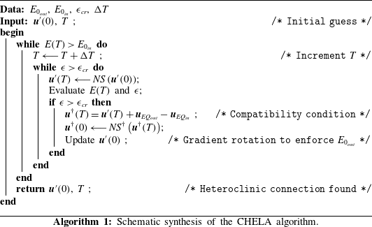
Technically, the algorithm consists of a double nested loop: an inner direct-adjoint loop for a fixed passage time, and an outer one increasing the passage time. Finding the minimal passage time by sequentially increasing
 $T$
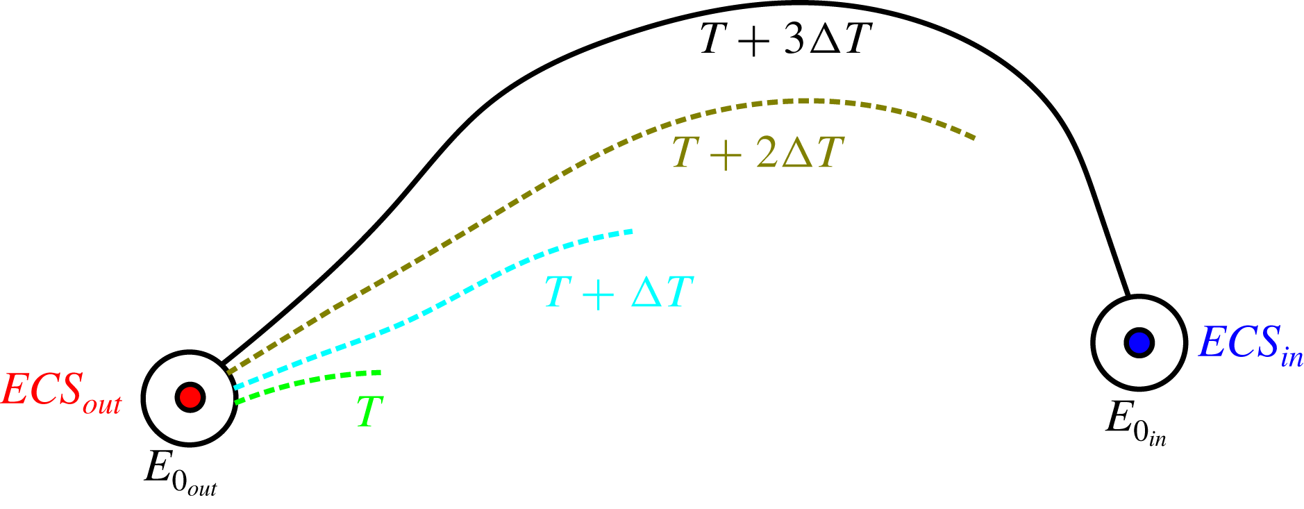
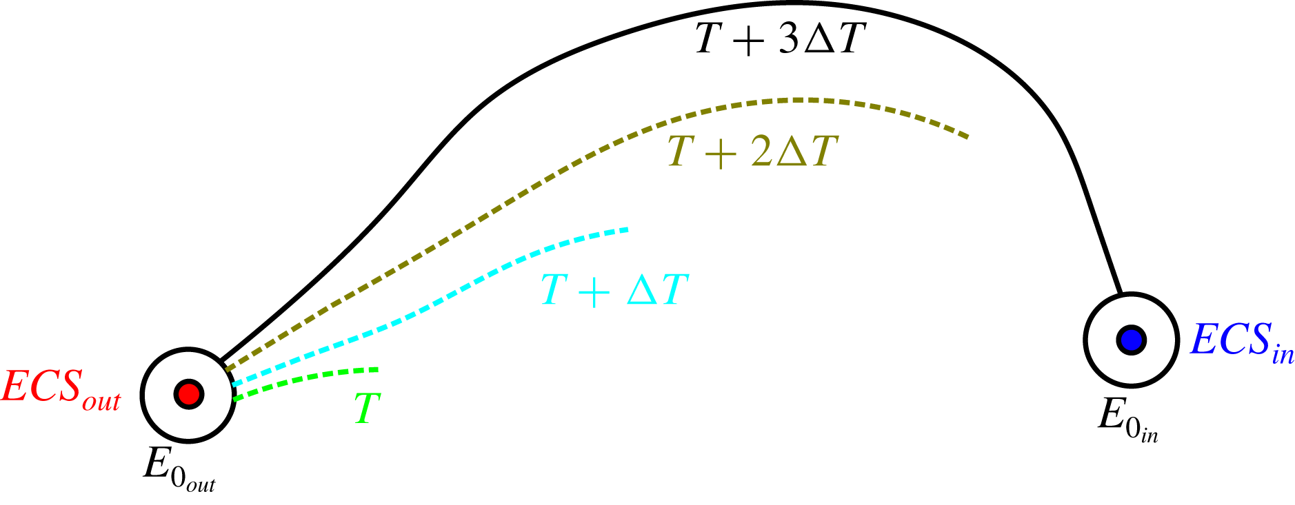
is a key element of the proposed CHELA (Computing HEteroclinic connections by using a Lagrange multiplier Algorithm) schematically presented in figure 1 and summarized in Algorithm 1. For a fixed passage time, the inner direct-adjoint loop is carried out until the relative difference of the value of
 $E(T)$
between successive iterations
 $\unicode[STIX]{x1D716}= ((E(T)^{n+1}-E(T)^{n})/E(T)^{n}$
is lower than a given threshold
 $\unicode[STIX]{x1D716}_{cr}$
, where superscript
 $n$
indicates the number of loop iterations. For short
 $T$
the trajectory will remain close to the initial equilibrium and not reach the neighbourhood of the final equilibrium, see dashed lines in figure 1. We therefore carry out the full optimization procedure for gradually increasing passage times
 $T$
(outer loop) until
 $E(T)<E_{0_{in}}$
and the trajectory reaches the neighbourhood of the final equilibrium, as indicated by the solid line in figure 1. By starting from a short passage time and increasing it, one avoids convergence problems of the direct-adjoint looping procedure stemming from chaotic dynamics that can lead to a non-smooth optimization problem at large passage times.
Sketch describing the CHELA algorithm: the initial condition and the related trajectory towards the final EQ change after updating the time
 $T$
(dashed lines). The algorithm stops when
 $T$
is sufficiently large to lead the flow field close enough to the final state (solid line).
We identify orbits connecting finite neighbourhoods of two equilibria in finite time, while a heteroclinic connection is traversed in infinite time. Especially in view of transient growth effects discussed below, considering finite neighbourhoods may lead to spurious results and the misidentification of heteroclinic connections. By analysing the dynamics in the neighbourhood of the initial and final equilibria we thus a posteriori confirm that every connection between finite neighbourhoods leaves the initial equilibrium shadowing its unstable manifold and approaches the final equilibrium along the stable one. Together, the variational method for constructing orbits connecting neighbourhoods of equilibria and the a posteriori check that those orbits shadow the unstable (stable) manifold of the initial (final) equilibrium allows one to approximate heteroclinic connections.
4 Results
In this section we present approximations to nine heteroclinic connections linking seven unstable equilibrium states originally found by Halcrow et al. (Reference Halcrow, Gibson, Cvitanović and Viswanath2009) and available in the Channelflow database (Gibson Reference Gibson2014). Seven connections are found for parameters
 $E_{0_{out}}=10^{-8}$
,
 $E_{0_{in}}=10^{-6}$
and
 $\unicode[STIX]{x1D716}_{cr}=10^{-4}$
. In terms of L2-distance this corresponds to shells of radius
 $r_{out}=10^{-4}$
and
 $r_{in}=10^{-3}$
. For two connections larger shells with
 $r_{out}=10^{-3}$
and
 $r_{in}=2.26\times 10^{-3}$
, corresponding to the values in Halcrow et al. (Reference Halcrow, Gibson, Cvitanović and Viswanath2009) are used. The larger shells reduce the passage time along the connections (underlined in table 1) and thereby avoid convergence problems of the optimization algorithm. As detailed below, we verify for all presented orbits that these shadow heteroclinic connections. First, we validated the algorithm by computing the three heteroclinic connections already found for plane Couette flow at
 $Re=400$
by Halcrow et al. (Reference Halcrow, Gibson, Cvitanović and Viswanath2009). Then, we found, for the same value of
 $Re$
, six previously unknown heteroclinic connections.
4.1 Connections identified and their properties
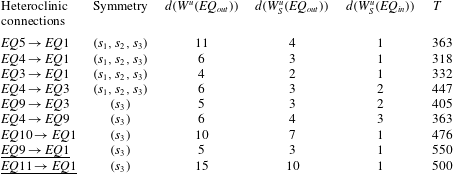
Details, specifically the dimension of the unstable manifold of the initial equilibrium, and the passage time
 $T$
, about the heteroclinic connections are given in table 1, where the equilibria are indicated following the same nomenclature employed by Gibson et al. (Reference Gibson, Halcrow and Cvitanović2009). The considered initial and final equilibria possess discrete symmetries which are part of the equivariance under a symmetry group. To construct a connecting trajectory within the symmetry subspace shared between initial and final equilibria, we explicitly constrain the time evolution to the shared symmetry subspace. The symmetry group considered here is
 $S=\{1,s_{1},s_{2},s_{3}\}$
and coincides with that of Gibson et al. (Reference Gibson, Halcrow and Cvitanović2008);
 $s_{1}$
and
 $s_{2}$
indicate the ‘shift-reflect’ and ‘shift-rotate’ symmetries, respectively, and
 $s_{3}=s_{1}s_{2}$
. Four of the considered equilibria have all the symmetries in
 $S$
, and the remaining ones have only
 $s_{3}$
. The first three connections coincide with those described by Halcrow et al. (Reference Halcrow, Gibson, Cvitanović and Viswanath2009).
Computed heteroclinic connections for
 $Re=400$
and corresponding symmetry subspaces. The dimension of the unstable manifold of the initial equilibrium (
 $EQ_{out}$
) is
 $d(W^{u})$
, while
 $d(W_{S}^{u})$
is the dimension of the intersection of the unstable manifold with the symmetry-invariant subspace reported here for the initial and final equilibrium (
 $EQ_{in}$
). The last column provides the passage time for the different orbits with shell around the initial state of radius
 $r_{out}=10^{-4}$
(
 $r_{out}=10^{-3}$
for underlined ones).
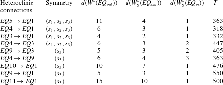
Two manifolds generically intersect if the sum of their dimensions is higher than or equal to the dimension of the state space they are embedded in (Halcrow et al.
Reference Halcrow, Gibson, Cvitanović and Viswanath2009). An intersection between the unstable manifold of the initial state and the stable one of the final state can thus generically exist if the codimension of the stable manifold in the
 $S$
-invariant space of the final state
 $d(W_{S}^{u}(EQ_{in}))$
is smaller than or equal to the dimension of the unstable manifold of the initial state
 $d(W_{S}^{u}(EQ_{out}))$
. This geometric condition is satisfied for all the computed heteroclinic connections (compare the fourth and fifth columns in table 1) and indicates the structural stability of all presented connections.
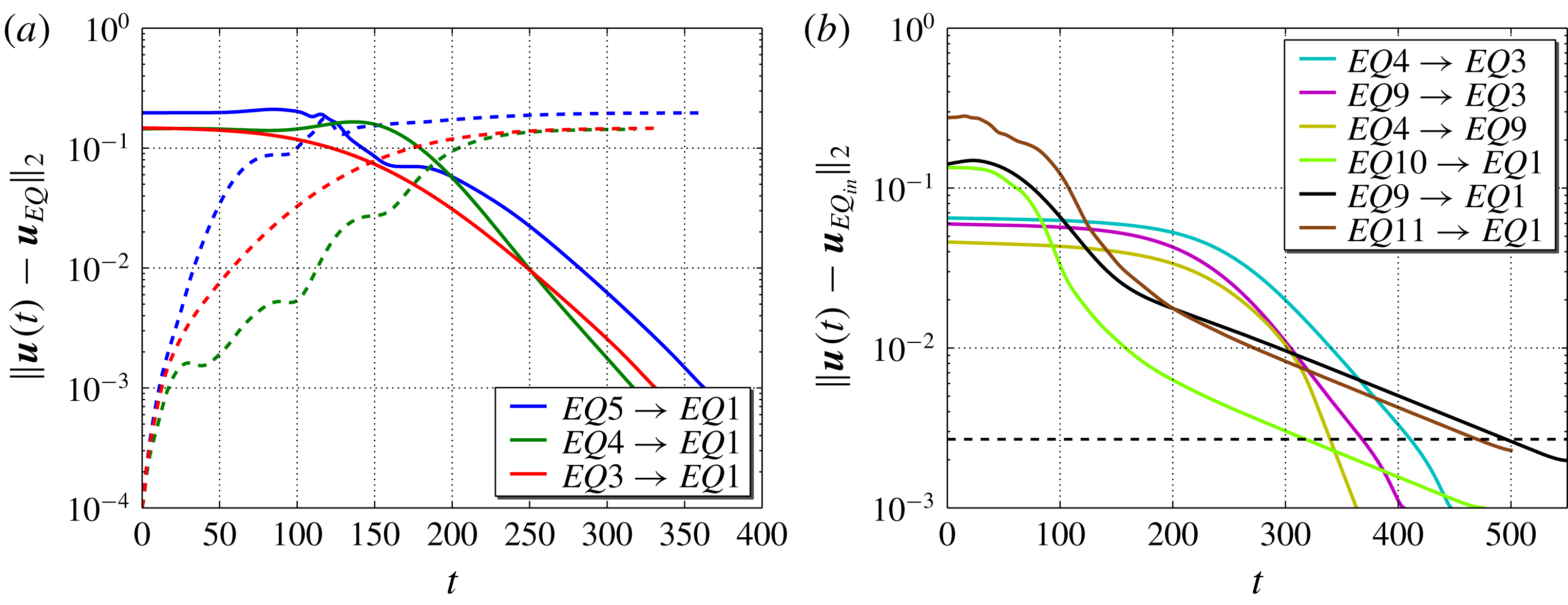
The convergence histories of the computed heteroclinic connections are shown in figure 2. For validation, panel (a) provides the distance of the velocity field
 $\boldsymbol{u}(t)$
to the target equilibrium
 $\boldsymbol{u}_{EQ_{in}}$
(continuous line) and to the initial equilibrium
 $\boldsymbol{u}_{EQ_{out}}$
(dashed line) for the three connections already obtained by Halcrow et al. (Reference Halcrow, Gibson, Cvitanović and Viswanath2009). For a fixed passage time
 $T$
and time increments,
 $\unicode[STIX]{x0394}T$
, chosen between 1 and 5 time units, the optimization algorithm typically requires 5 to 20 forward/backward time integrations to converge. The convergence curves are in good agreement with those obtained in the literature, with the convergence threshold achieved by Halcrow et al. (Reference Halcrow, Gibson, Cvitanović and Viswanath2009) indicated by a dashed line in figure 2(b).
(a) Distances of the velocity field
 $\boldsymbol{u}(t)$
to the final equilibrium
 $\boldsymbol{u}_{EQ_{in}}$
(continuous line) and to the initial one
 $\boldsymbol{u}_{EQ_{out}}$
(dashed line) along three heteroclinic connections found by Halcrow et al. (Reference Halcrow, Gibson, Cvitanović and Viswanath2009) versus time. (b) Distances to the final equilibrium
 $\boldsymbol{u}_{EQ_{in}}$
for the new computed heteroclinic connections (continuous lines). The dashed line represents the highest residual value for the heteroclinic connections computed in Halcrow et al. (Reference Halcrow, Gibson, Cvitanović and Viswanath2009). The L2-norm of the considered equilibria ranges from 0.1259 to 0.4049. (Gibson et al.
Reference Gibson, Halcrow and Cvitanović2009).
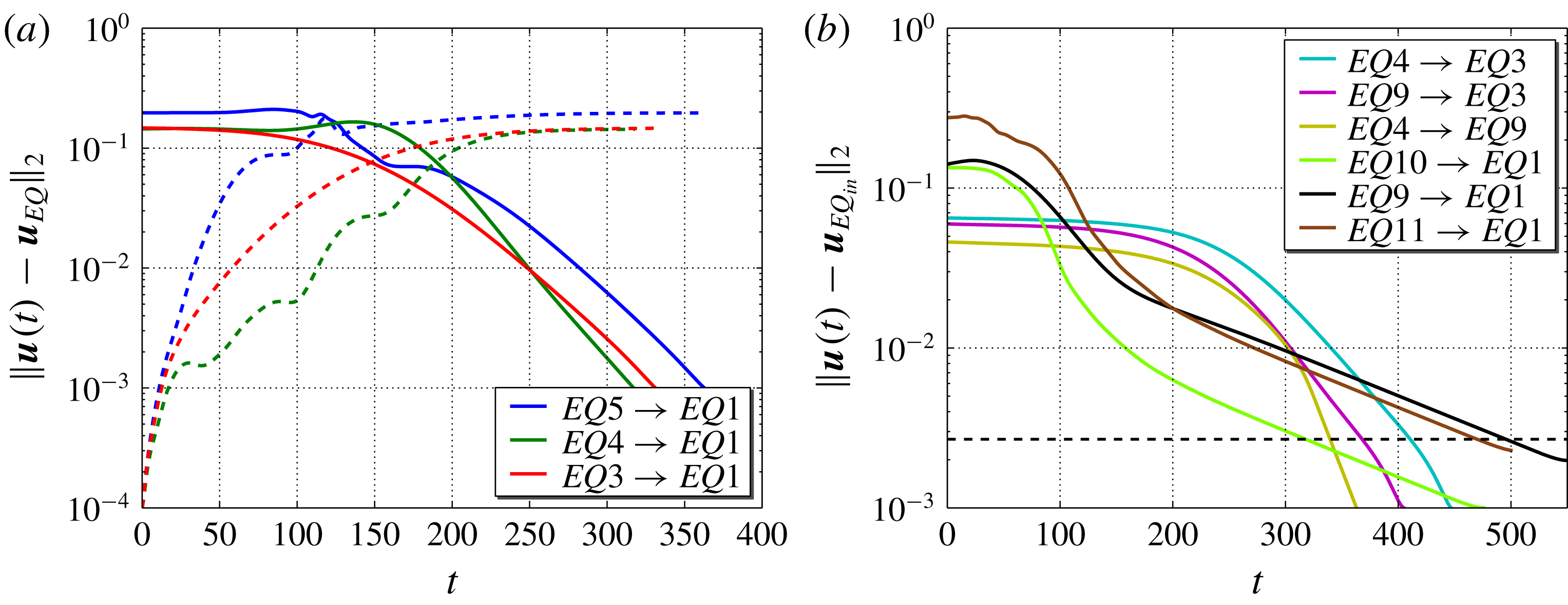
Figure 2(b) shows the new six heteroclinic connections computed here. Three of the new connections lead to the edge state (Nagata Reference Nagata1990; Schneider et al.
Reference Schneider, Gibson, Lagha, De Lillo and Eckhardt2008), two of them to
 $EQ3$
, and one to
 $EQ9$
. All connections reported by Halcrow et al. (Reference Halcrow, Gibson, Cvitanović and Viswanath2009) land on the codimension-1 stable manifold of the edge state, which simplifies identifying those connections using a one-dimensional search algorithm. The variational method proposed here yields additional connections not involving the edge state.
4.2 Confirming that computed orbits shadow heteroclinic connections
Heteroclinic connections lie in the intersection of the unstable manifold of the initial equilibrium and the stable manifold of the final equilibrium. The use of finite energy shells renders the passage time along the orbit finite but may potentially lead to spurious results. A specific problem is due to transient growth effects that may allow a trajectory to leave the neighbourhood of an equilibrium along an algebraically amplified direction bypassing the unstable manifold (Farano et al.
Reference Farano, Cherubini, Robinet, De Palma and Schneider2018). We thus analyse the dynamics close to the equilibria where curved stable and unstable manifolds can be approximated by their respective tangent spaces, the stable and unstable subspaces spanned by the stable or unstable eigenvectors of the Navier–Stokes equations linearized around the equilibrium. The analysis of the orbits connecting finite energy shells technically involves two steps: first, along the orbit we determine the range in the vicinity of both equilibria, where the dynamics is well approximated by the Navier–Stokes equations linearized around
 $EQ_{out}$
or
 $EQ_{in}$
, respectively. This is achieved by explicitly comparing the nonlinear and the linear time evolution. Within the validity range of the linearization, we then project onto an orthonormal basis of the unstable tangent spaces to the invariant manifolds of both equilibria and thereby separate the energetic contributions in the stable and unstable subspaces approximating the respective manifolds. (Note that we technically only use projections on the unstable subspace spanned by the orthogonalized unstable eigenvectors. These leading eigenvectors can be accurately constructed by our iterative Arnoldi method, while most of the stable eigenvectors are challenging to compute accurately using matrix-free techniques.)
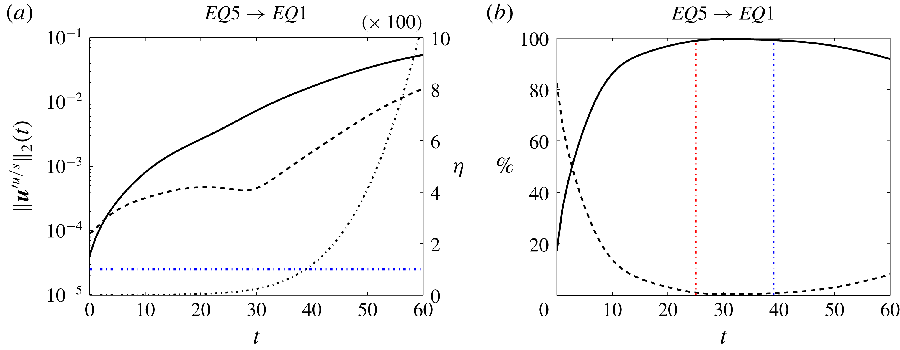
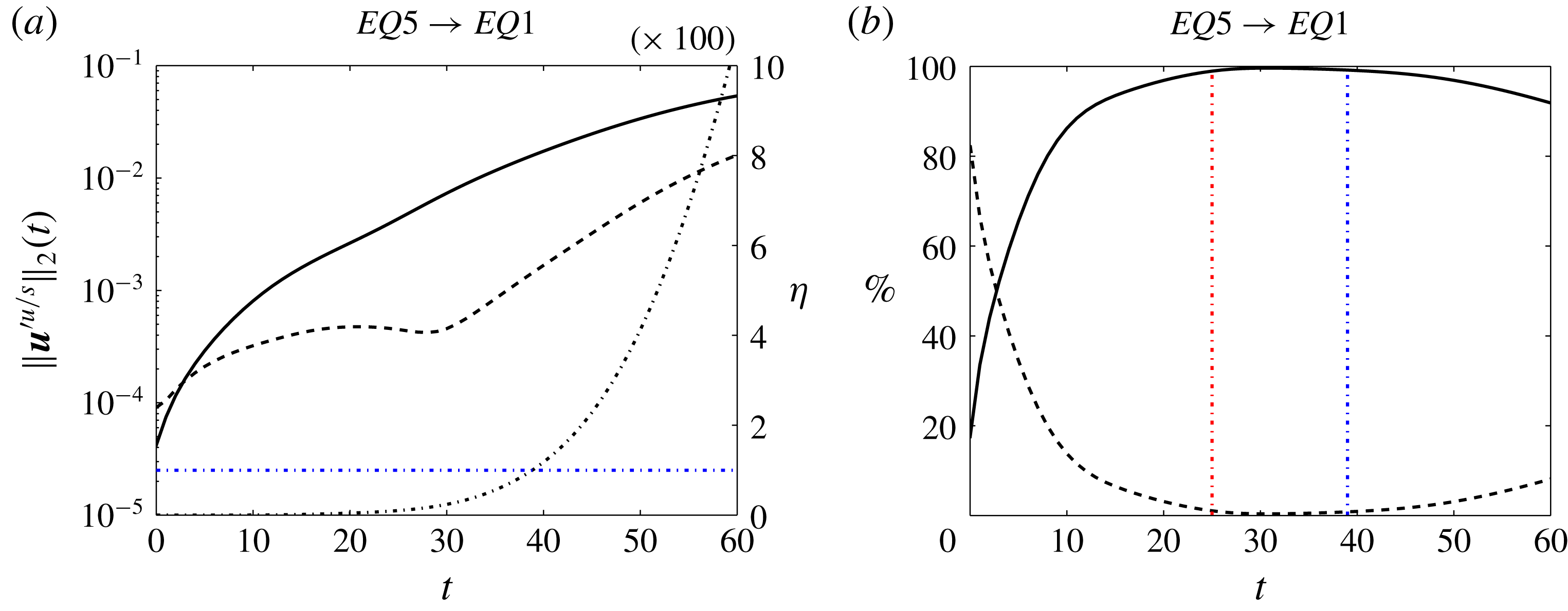
Time evolution of contributions in the stable and unstable subspaces of
 $EQ_{out}$
during the initial part of the trajectory
 $EQ5\rightarrow EQ1$
. (a) L2-norms
 $\Vert \boldsymbol{u}^{\prime \,s/u}\Vert _{2}$
of the projections onto the unstable (
 $\boldsymbol{u}^{\prime \,u}$
, solid line) and stable (
 $\boldsymbol{u}^{\prime \,s}$
, dashed line) subspace. The difference between the linearized and the full nonlinear evolution
 $\unicode[STIX]{x1D702}=(\Vert \boldsymbol{u}_{lin}^{\prime }(t)-\boldsymbol{u}^{\prime }(t)\Vert _{2}^{2}/\Vert \boldsymbol{u}_{lin}^{\prime }(t)\Vert _{2}^{2})$
(dotted line, right axis) characterizes the deviation of the invariant manifolds from the approximating linear subspaces due to manifold curvature in the direction of the trajectory. (b) Relative contribution measured in terms of relative energy in the unstable (solid line) and stable (dashed line) subspace. Vertical red dotted lines indicates when the relative contribution of the stable subspace
 $E^{s}(t)/E(t)$
drops below 1 %. Vertical blue dotted line indicates when the difference between the linearized and the full nonlinear evolution
 $\unicode[STIX]{x1D702}$
reaches 1 %.
For all identified orbits connecting finite energy shells of radius
 $r_{out}=10^{-4}$
,
 $r_{in}=10^{-3}$
, the identified initial condition lies predominantly in the stable subspace of
 $EQ_{out}$
, with relative energy in the stable versus unstable space ranging from 82 % to 98 %. To follow the evolution of the contributions we decompose
 $\boldsymbol{u}^{\prime }(t)=\boldsymbol{u}^{\prime \,u}(t)+\boldsymbol{u}^{\prime \,s}(t)$
into components in the stable/unstable subspace. Figure 3(a) shows the time evolution of the L2-norm of the contributions within the stable/unstable subspace of the orbit while leaving
 $EQ_{out}$
for the connection
 $EQ5\rightarrow EQ1$
. Data for other connections is provided in the supplementary material available at https://doi.org/10.1017/jfm.2018.860. Both
 $\Vert \boldsymbol{u}^{\prime \,u}\Vert _{2}(t)$
and
 $\Vert \boldsymbol{u}^{\prime \,s}\Vert _{2}(t)$
initially increase. The growth of the stable contribution slows down and starts to decay, while in the unstable subspace sustained approximately exponential growth continues. If the dynamics were linear, we would expect the stable contribution to decay to zero. However, due to the curvature of the invariant manifolds, the projection on the stable subspace may grow again, when the stable subspace no longer well approximates the attracting curved stable manifold. This is evidenced by the subsequent growth of
 $\Vert \boldsymbol{u}^{\prime \,s}\Vert _{2}(t)$
starting at
 $t\approx 30$
when the deviation between linear and nonlinear evolution
 $\unicode[STIX]{x1D702}=(\Vert \boldsymbol{u}_{lin}^{\prime }(t)-\boldsymbol{u}^{\prime }(t)\Vert _{2}^{2}/\Vert \boldsymbol{u}_{lin}^{\prime }(t)\Vert _{2}^{2})$
starts to increase. We thus observe transient growth in the stable subspace which is superseded by exponential growth along the unstable subspace. Consequently, the trajectory shows a transient excursion along the stable subspace, but eventually the orbit approaches the unstable subspace, as evidenced by the decaying relative contribution of the stable subspace (see figure 3
b). This decay is observed during the initial part of the orbit and while the unstable subspace remains a good approximation of the unstable manifold describing the nonlinear dynamics (see vertical blue dotted line in figure 3
b, and dotted line in figure 3
a). For all connections found for a shell of radius
 $r_{out}=10^{-4}$
the contribution of
 $\boldsymbol{u}^{\prime }$
in terms of energy in the unstable subspace reaches more than 99 % while the relative difference between the linear and nonlinear evolution
 $\unicode[STIX]{x1D702}$
remains bounded by 0.858 %. (Alternatively, when the ratio of L2-norms reaches
 $\Vert \boldsymbol{u}^{\prime \,u}\Vert _{2}>0.99\Vert \boldsymbol{u}^{\prime }\Vert _{2}$
,
 $\sqrt{\unicode[STIX]{x1D702}}$
remains bounded by 7.23 %.) The analysis consisting of projecting onto the stable subspace and monitoring the deviation between linear and nonlinear time evolution thus strongly supports the following interpretation: during the initial part, the orbit identified by the optimization algorithm does not follow the unstable manifold of
 $EQ_{out}$
, but rather exploits algebraic growth along transiently amplified directions predominantly in the stable manifold. However, after a short excursion along the stable manifold, the orbit approaches the unstable manifold and shadows a heteroclinic connection.
For two orbits
 $EQ9\rightarrow EQ1$
and
 $EQ11\rightarrow EQ1$
the passage time is too large for the optimization to converge if a small energy shell of radius
 $r_{out}=10^{-4}$
is chosen. For the connection
 $EQ9\rightarrow EQ1$
and shell of radius
 $r_{out}=10^{-3}$
, the contributions of
 $\boldsymbol{u}^{\prime }$
in terms of relative energy in the unstable subspace reach 99 % while
 $\unicode[STIX]{x1D702}$
remains bounded by 0.763 %. For the orbit
 $EQ11\rightarrow EQ1$
a strongly curved unstable manifold renders the linearization invalid after a short time and before the relative contribution in terms of energy (L2-norm) of the unstable manifold has reached 61 % (78 %). However, the contraction rate along the stable subspace is similar to that observed for all other orbits. This suggests that despite the importance of nonlinear effects the orbit follows the strongly curved unstable manifold when leaving
 $EQ_{out}$
.
An analogous analysis of the dynamics linearized around
 $EQ_{in}$
confirms that all orbits approach the final equilibria along their stable manifold. Consequently, the orbits connecting finite shells around two equilibria follow the unstable manifold of
 $EQ_{out}$
and the stable one of
 $EQ_{in}$
. The initial part of the orbit is affected by transient amplification in the stable manifold, but the excursion decays before an L2-distance from
 $EQ_{out}$
of order
 $10^{-2}$
–
 $10^{-3}$
is reached. More importantly, this distance is small compared to the typical L2-norm of the distance between both connected equilibria. The ratio of the distance affected by transient amplification to distance between both equilibria ranges from
 $0.016$
to
 $0.100$
. Consequently, the orbit shadows the heteroclinic connections along at least 90 % of the distance between equilibria. Data for the individual connections are given in the supplementary material.
We verify that the computed orbits are robust to changes of the size of the initial energy shell. All orbits available for
 $r_{out}=10^{-4}$
were successfully recomputed for a larger shell of radius
 $r_{out}=10^{-3}$
. For connections where the dimension of the intersection of the unstable manifold of the initial equilibrium with the stable manifold of the final state is greater than one, e.g.
 $EQ4\rightarrow EQ1$
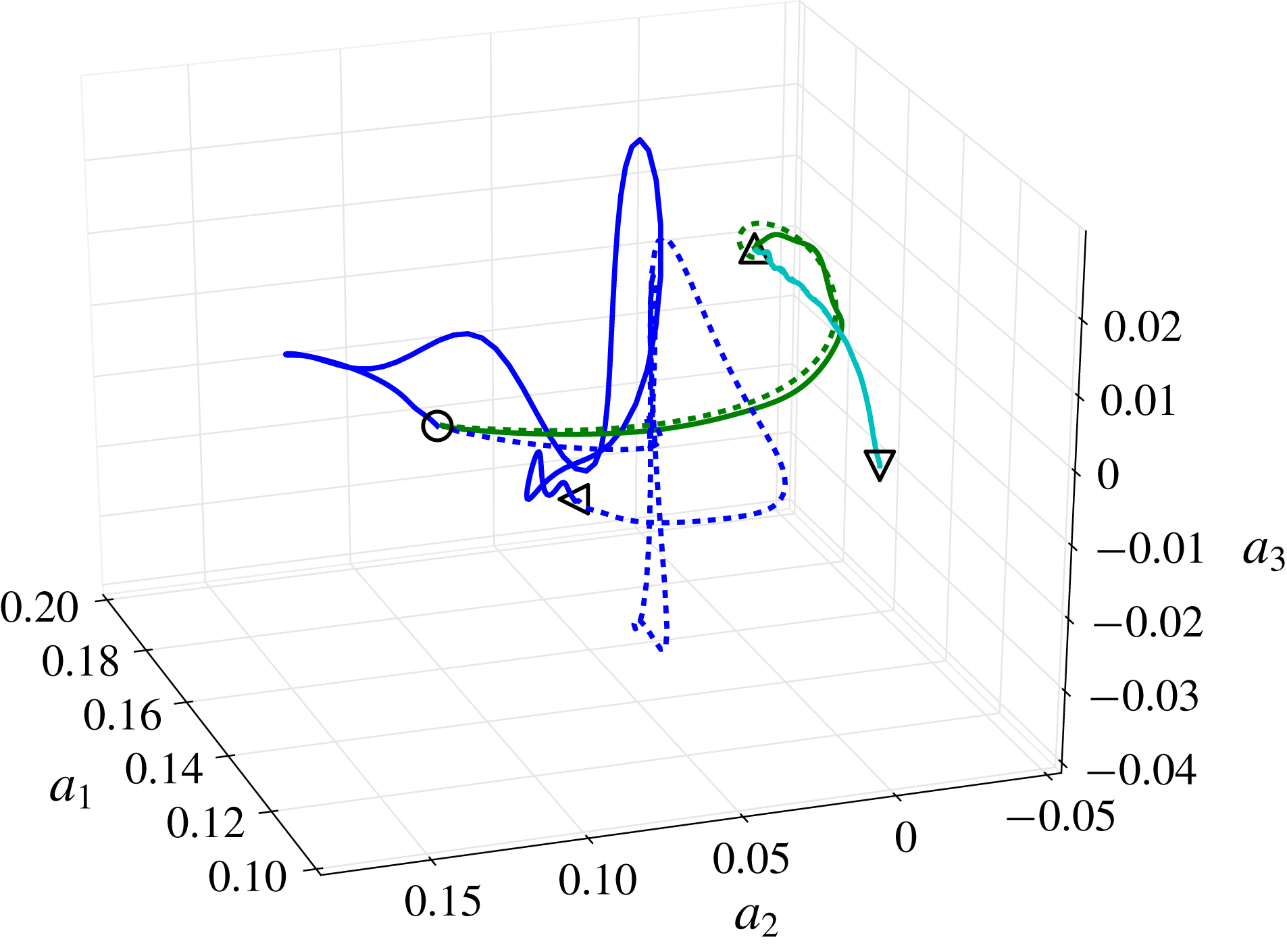
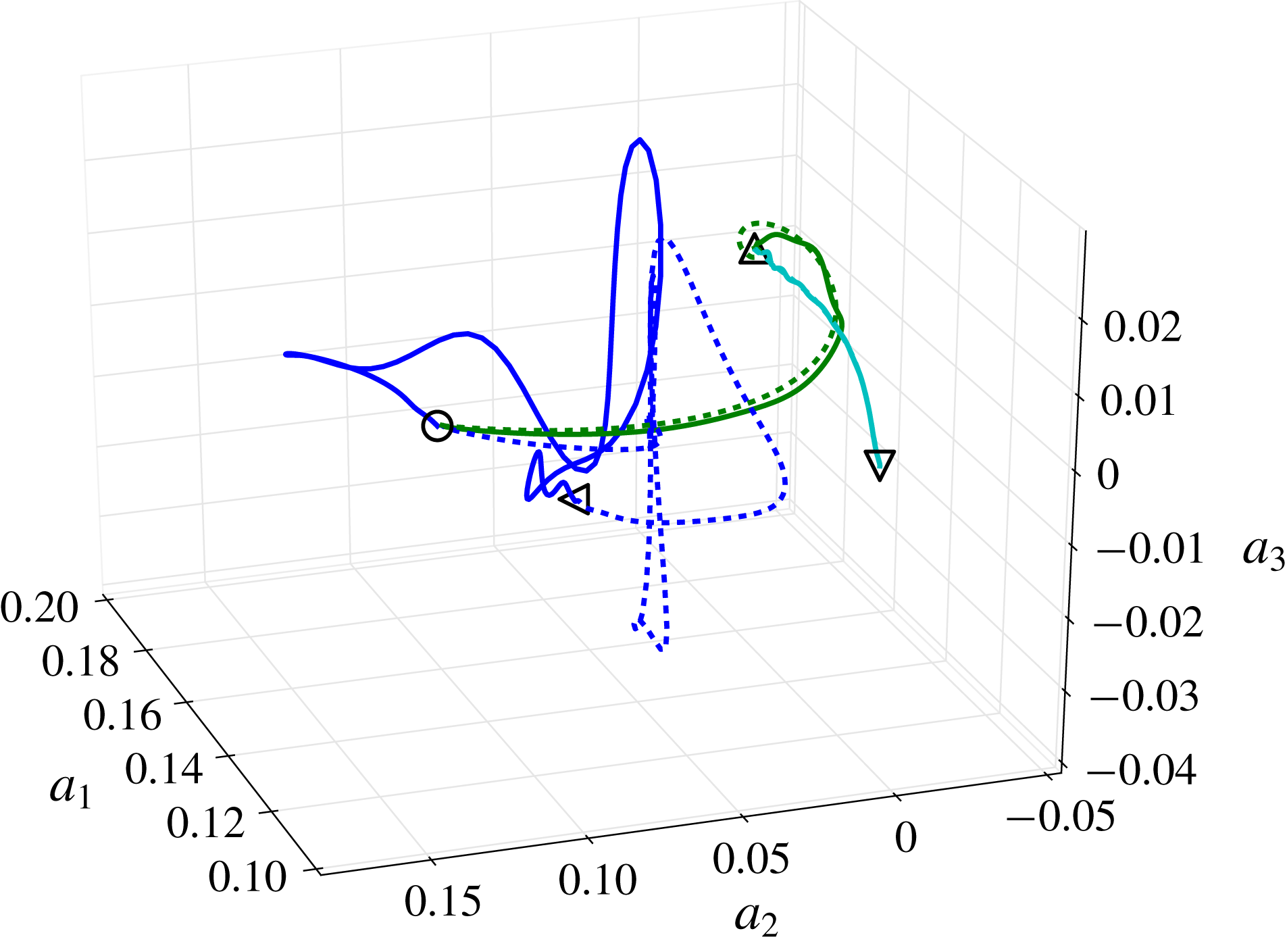
, there is a continuous family of connections between these two states. Consequently, varying the energy shell may yield slightly different connections within the continuum. Likewise, the constrained search in Halcrow et al. (Reference Halcrow, Gibson, Cvitanović and Viswanath2009) yields a specific connection, while the variational algorithm may find a different connection within the continuum. For all connections with one-dimensional intersection, independently of the energy shell, the algorithm always converges to the only existing connection. This is demonstrated in figure 4 for the orbit
 $EQ4\rightarrow EQ3$
.
State-space projection (Gibson et al.
Reference Gibson, Halcrow and Cvitanović2008) of the orbit connecting
 $EQ5\rightarrow EQ1$
(blue) and
 $EQ4\rightarrow EQ1$
(green), for which the dimension of the intersection is three and two, respectively. For a specific connection, changing the energy shell around the initial equilibrium from
 $E_{0_{out}}=10^{-6}$
(solid line) to
 $E_{0_{out}}=10^{-8}$
(dashed line) results in finding different orbits. For those connections for which the dimension of the intersection is one, g.e.
 $EQ4\rightarrow EQ3$
(cyan), the algorithm finds the only existing connection.
4.3 Connectivity of equilibrium states
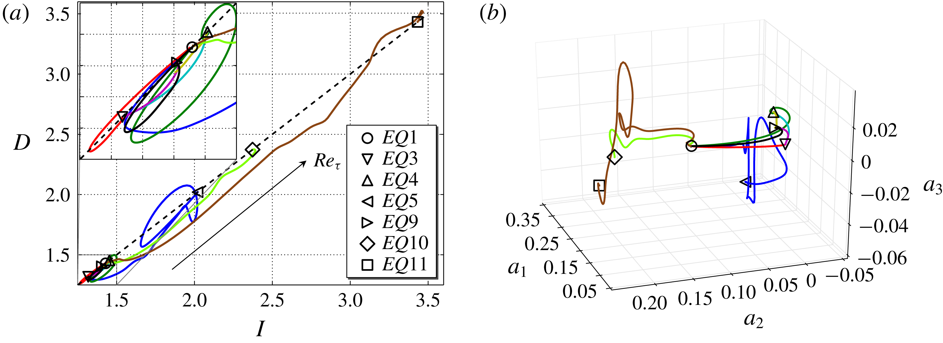
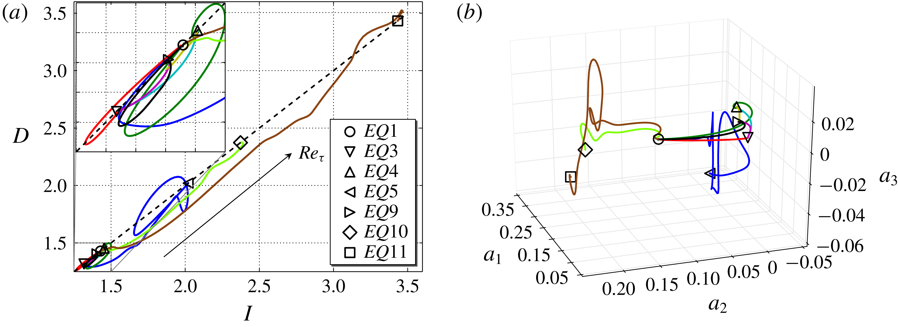
When visualizing the computed heteroclinic connections in the energy input (
 $I$
) versus dissipation rate (
 $D$
) plane (Kawahara & Kida Reference Kawahara and Kida2001) (figure 5
a) one observes that most orbits are located in the vicinity of the edge state equilibrium
 $EQ1$
. With the exception of
 $EQ10$
and
 $EQ11$
all other connected equilibria have a lower dissipation than the average value
 $D=I\approx 2.5$
for long turbulent transients (Cherubini & De Palma Reference Cherubini and De Palma2014). Along the majority of all connections – with exceptions
 $EQ3\rightarrow EQ1$
,
 $EQ9\rightarrow EQ1$
– the friction Reynolds number
 $Re_{\unicode[STIX]{x1D70F}}$
decreases, indicating that turbulent fluctuations are reduced along the orbit. This suggests that the presented heteroclinic connections are more relevant for relaminarization processes than the turbulent dynamics itself. Of special interest is the trajectory
 $EQ11\rightarrow EQ1$
, involving
 $EQ11$
with dissipation well above the turbulent mean. This trajectory captures features of turbulent bursting.
To better visualize how the EQs are mutually connected, the heteroclinic connections are also plotted using the 3D orthonormal projection of the state space proposed by Gibson et al. (Reference Gibson, Halcrow and Cvitanović2008). The time series of the projection coefficients
 $(a_{1}(t),a_{2}(t),a_{3}(t))$
are obtained using the inner product
 $a_{i}(t)=\langle \boldsymbol{u}(t),\boldsymbol{e}_{i}\rangle$
defined above, where
 $i=1,2,3$
and
 $\boldsymbol{e}_{i}$
are the orthonormal basis functions based on
 $EQ2$
and its half-cell translated siblings (Gibson et al.
Reference Gibson, Halcrow and Cvitanović2008). The resulting trajectories projected onto this reduced basis are reported in figure 5(b). Within the network of heteroclinic connections, the edge state
 $EQ1$
is centrally located. For all other equilibrium states there is a direct connection landing on
 $EQ1$
. This indicates that all the considered equilibria are states on the edge of chaos, characterizing the dynamics on the stable manifold of the edge state. This is consistent with the edge of chaos and the chaotic saddle being dynamically linked for the considered domain size and Reynolds number (Chantry & Schneider Reference Chantry and Schneider2014). The flow evolution along the newly constructed heteroclinic connections are discussed in the supplementary material, where we also provide flow visualizations for all connections (see the supplementary movie).
(a) Projection of the heteroclinic connections onto the energy input,
 $I$
, and the dissipation rate,
 $D$
, normalized by their value in the laminar flow. (b) State-space projection onto the 3D orthonormal basis
 $\boldsymbol{a}_{1,2,3}$
of all the computed heteroclinic connections. Colours are the same as in figure 2.
5 Discussion and outlook
In this work, we develop a variational method based on nonlinear minimization techniques to identify heteroclinic connections between equilibrium states. The variational method complements alternative shooting methods employed previously. A shooting method aims at finding an initial condition in the unstable manifold of the initial equilibrium that reaches the final one. This approach is only feasible for unstable manifolds of very low dimension to limit the search space, and also requires the manifold curvature to be negligible so that a linear combination of unstable eigenvectors approximates a perturbation of the initial equilibrium located in the unstable manifold. Specifically, Halcrow et al. (Reference Halcrow, Gibson, Cvitanović and Viswanath2009) consider perturbations spanned by only two specifically chosen unstable eigenvectors, which yields a one-parameter search problem. The alternative approach by Van Veen et al. (Reference Van Veen, Kawahara and Atsushi2011), based on work by Krauskopf et al. (Reference Krauskopf, Osinga, Doedel, Henderson, Guckenheimer, Vladimirsky, Dellnitz and Junge2005), Krauskopf & Osinga (Reference Krauskopf and Osinga2007), treats the search for heteroclinic connections as a boundary-value problem (BVP). The BVP is underdetermined, and a one-parameter family of solutions covering a part of the unstable manifold can be found by arclength continuation. This method is very accurate and robust, but it is limited to 2D unstable manifolds.
Compared to these alternative methods, the variational approach proposed here has several advantages: first, there is no constraint on the dimensionality of unstable manifolds and no ad hoc assumptions for a suitable reduced search space are necessary. Rather, the variational approach explores initial conditions within the full space. The proposed method allows one to approximate heteroclinic connections originating from states with multi-dimensional unstable manifold and thereby provides access to connections that cannot easily be identified with alternative methods. Three computed connections that do not land on the edge state (
 $EQ4\rightarrow EQ3$
,
 $EQ9\rightarrow EQ3$
and
 $EQ4\rightarrow EQ9$
) are examples of connections that are hard to identify using shooting methods, but can easily be found with the proposed variational method. Second, larger energy shells can be considered as there is no necessity for the unstable manifold to be well approximated by the unstable subspace which shooting methods constrain their search to.
While using a variational method to construct connections between finite energy shells removes constraints on the dimensionality of the unstable manifold of the initial equilibrium, the approach has some limitations. To avoid convergence issues the size of the energy shells should be sufficiently large to limit the transit time along the connection. Thereby the exponentially amplified dependence on initial conditions in the chaotic system can be controlled and the optimization problem remains smooth enough for the iterative algorithm to converge. However, as a consequence of using finite energy shells, the algorithm may produce spurious results, since a connection between finite shells is not guaranteed to shadow a heteroclinic connection located within the intersection of the unstable manifold of the starting and the stable manifold of the final equilibrium. Consequently, a careful a posteriori analysis of the dynamics close to the two equilibria is an integral and unavoidable step to confirm that a computed orbit shadows a heteroclinic connections. Furthermore, due to transient growth effects, the initial part of the identified orbit may not shadow the heteroclinic connection. For all examples presented here, we observed this initial part to be short (less than 10 % of the distance between equilibria) so that the constructed orbits between finite shells shadow heteroclinic connections along almost their full length.
In conclusion, the variational method has the disadvantage that a careful analysis of orbits between energy shell is needed to ensure that those approximate heteroclinic connections. However, the advantage is that the new method gives access to heteroclinic connections which cannot be easily computed using alternative techniques.
Supplementary material and movie
Supplementary material and a movie are available at https://doi.org/10.1017/jfm.2018.860.