1. Introduction
Laminar–turbulent transition in hypersonic boundary layers poses a fundamental challenge in aerodynamic designs of high-speed flying vehicles. As the surface friction and heat flux undergo remarkable increase during the transition process, employing effective control strategies to delay the transition onset is favourable in the sense of reducing the total drag and thermal load.
Depending on the intensity of environmental perturbations, boundary-layer transition can follow several routes (Morkovin Reference Morkovin1968). Among these, natural transition, occurring under conditions of low environmental perturbations, is frequently encountered by cruising hypersonic vehicles. This process is initiated by small-amplitude normal modes through a receptivity mechanism, followed by exponential amplification due to the linear instability mechanism. According to linear stability theory (LST) (Mack Reference Mack1975), multiple instability modes exist within two-dimensional (2-D) hypersonic boundary layers, known as the Mack first, second and higher-order modes, listed in order of increasing frequency. Asymptotic analyses have indicated that only the first mode, with an oblique wave angle exceeding
 $\tan ^{-1}(\sqrt {M^2-1})$
(where
 $M$
denotes the Mach number), possesses viscous feature (Smith Reference Smith1989; Liu, Dong & Wu Reference Liu, Dong and Wu2020), while the quasi-2-D Mack first mode and all higher-order modes are inviscid (Cowley & Hall Reference Cowley and Hall1990; Smith & Brown Reference Smith and Brown1990; Dong, Liu & Wu Reference Dong, Liu and Wu2020). A thorough review of studies addressing the receptivity and linear evolution of Mack modes can be found in Fedorov (Reference Fedorov2011) and Zhong & Wang (Reference Zhong and Wang2012). As the normal modes accumulate to finite amplitudes, the nonlinear interactions among different Fourier components become increasingly significant, eventually leading to a transition to turbulence. As reviewed by Herbert (Reference Herbert1988) and Kachanov (Reference Kachanov1994) for incompressible boundary layers, three types of nonlinear mechanisms have been identified: (a) fundamental resonance occurring between a primary 2-D mode and a pair of secondary oblique modes sharing the same frequency as the 2-D mode; (b) subharmonic resonance arising between a primary 2-D mode and a pair of secondary oblique modes with a common frequency that is half that of the 2-D mode; and (c) oblique breakdown occurring between two dominant oblique modes with opposite spanwise wavenumbers. Given the three-dimensional (3-D) nature of the dominant Mack first mode, oblique breakdown frequently occurs in low-Mach-number supersonic boundary layers. In contrast, the 2-D Mack second mode exhibits greater instability, and numerous numerical studies have identified fundamental resonance as the most likely mechanism to trigger hypersonic boundary-layer transition (Li et al. Reference Li, Choudhari, Chang and White2012; Sivasubramanian & Fasel Reference Sivasubramanian and Fasel2014; Hader & Fasel Reference Hader and Fasel2019; Unnikrishnan & Gaitonde Reference Unnikrishnan and Gaitonde2020).
Over the past few decades, researchers have focused on delaying the onset of transition by suppressing perturbation evolution during the linear phase through various control strategies. Early experimental studies (Holloway & Sterrett Reference Holloway and Sterrett1964; Fujii Reference Fujii2006) reported a potentially effective control strategy involving the implementation of 2-D isolated roughness in the laminar phase of a hypersonic boundary layer, which stands in contrast to low-speed configurations. Subsequent numerical studies by Fong et al. (Reference Fong, Wang and Zhong2014, Reference Fong, Wang, Huang, Zhong, McKiernan, Fisher and Schneider2015) confirmed this phenomenon, demonstrating that the Mack second mode can be stabilised by roughness placed downstream of the synchronisation point where the fast and slow modes intersect. However, if the roughness is located upstream of the synchronisation point, or if the dominant perturbation frequency is lower than the synchronisation frequency for a fixed roughness location, the Mack mode could be enhanced. A systematic numerical study conducted by Zhao, Dong & Yang (Reference Zhao, Dong and Yang2019) employed the harmonic linearised Navier–Stokes (HLNS) approach to reveal the impact of roughness on Mack modes across the entire frequency spectrum. This mechanism was further elucidated by Dong & Zhao (Reference Dong and Zhao2021) using high-Reynolds-number asymptotic analysis. Other surface imperfections such as steps and distributed wavy walls influence the Mack-mode evolution through the same mechanism. While direct numerical simulations (DNSs) (Egorov, Novikov & Fedorov Reference Egorov, Novikov and Fedorov2010; Zhu et al. Reference Zhu, Gu, Si, Zhang, Chen, Smith, Zhu and Lee2022; Liu et al. Reference Liu, Yang, Tu, Li, Guo and Wan2023) and experiments (Bountin et al. Reference Bountin, Chimitov, Maslov, Novikov, Egorov, Fedorov and Utyuzhnikov2013; Si et al. Reference Si, Huang, Zhu, Chen and Lee2019; Xu et al. Reference Xu, Yi, Quan, Lu and Han2022) have confirmed that steps and wavy walls effectively delay transition under certain conditions, the robustness of such control strategies remains uncertain.
A notable passive control approach involves the use of porous coatings with microholes, which have received attention for their capacity to influence the evolution of Mack second modes without causing significant mean-flow distortions. Given that the Mack second mode exhibits pressure perturbations with acoustic-wave characteristics, these porous coatings facilitate the propagation and reflection of acoustic waves through the microholes, effectively altering the phase and amplitude of the second mode. By employing an admittance boundary condition to represent the effects of the porous surface, Fedorov (Reference Fedorov2003) demonstrated that porous coatings effectively suppress the growth rate of the second mode across a broad frequency range. These findings have been confirmed by various studies, including theoretical (Fedorov et al. Reference Fedorov, Kozlov, Shiplyuk, Maslov and Malmuth2006), numerical (Sandham & Lüdeke Reference Sandham and Lüdeke2009; Sousa et al. Reference Sousa, Patel, Chapelier, Wartemann, Wagner and Scalo2019; Zhao et al. Reference Zhao, Dong, Zhang, Wen, Long and Yuan2021; Song & Zhao Reference Song and Zhao2022) and experimental investigations (Maslov et al. Reference Maslov, Shiplyuk, Sidorenko, Polivanov, Fedorov, Kozlov and Malmuth2006; Miller et al. Reference Miller, Mamrol, Redmond, Jantze, Scalo and Jewell2022). A comprehensive review of this topic can be found in Zhao et al. (Reference Zhao, Wen, Zhou, Tu and Lei2022). Gaponov (Reference Gaponov2014) further extended this research by exploring variable wall admittance boundary conditions for hypersonic boundary layers over a flexible membrane covering on a porous wall, achieving enhanced stabilisation effects within specific frequency bands. Recognising the effectiveness of this control strategy in the downstream region, Ji, Dong & Zhao (Reference Ji, Dong and Zhao2023) conducted a focused study on the scattering of Mack modes at the interface between rigid and compliant walls.
Imposing blowing and suction at the wall is regarded as a representative active control strategy for delaying transition in boundary-layer flows. Local suction has been shown to suppress Tollmien–Schlichting modes in incompressible boundary layers (Reed & Nayfeh Reference Reed and Nayfeh1986). However, its effects on the hypersonic Mack second mode can differ for high and low frequencies (Wang & Lallande Reference Wang and Lallande2020; Poulain et al. Reference Poulain, Content, Rigas, Garnier and Sipp2024), which can be explained by the same mechanism identified by Dong & Zhao (Reference Dong and Zhao2021). Utilising combined steady blowing and suction strips with a strong magnitude, Hader & Fasel (Reference Hader and Fasel2021, Reference Hader and Fasel2024) and Zhuang et al. (Reference Zhuang, Wan, Liu, Sun and Lu2024) conducted DNS to investigate their impact on transition in hypersonic boundary layers. They found that the strong blowing and suction velocities induce significant mean-flow distortion, leading to a stabilising effect on the Mack second mode. This effect was confirmed to effectively delay transition in the cases examined. Additionally, Zhuang et al. (Reference Zhuang, Wan, Ye, Luo, Liu, Sun and Lu2023) explored a combined unsteady blowing and suction slot with a strong magnitude, referred to as a synthetic jet. Their studies observed a delayed transition due to its stabilising effect on the fundamental mode during the linear phase.
Early numerical studies (Mack Reference Mack1984) demonstrated that reducing wall temperature generally destabilises the second mode in the high-frequency band while stabilising the low-frequency second mode and the first mode. Conversely, increasing wall temperature has the opposite effect. This observation has prompted researchers to explore surface heating or cooling as another representative active control strategy. Fedorov et al. (Reference Fedorov, Ryzhov, Soudakov and Utyuzhnikov2014) introduced a local volume heating strategy to study its impact on hypersonic boundary-layer transition through DNSs. They found that when the heating source is positioned upstream of the neutral point, the second mode is stabilised; however, a scattering effect is observed when the heating source is located downstream. Subsequent numerical (Zhao et al. Reference Zhao, Wen, Tian, Long and Yuan2018; Oz et al. Reference Oz, Goebel, Jewell and Kara2023) and theoretical (Zhao & Dong Reference Zhao and Dong2022) studies reported that surface cooling strips can stabilise Mack-mode evolution when placed upstream of a critical point, whereas surface heating strips can stabilise the Mack mode when positioned downstream of this critical point. Notably, the critical point was identified as being close to the location where the second mode reaches its maximum growth rate (Zhao & Dong Reference Zhao and Dong2022; Park et al. Reference Park, Rajendran, Kim, Lim, Jee and Park2023). In addition to these theoretical and numerical insights, Oz & Kara (Reference Oz and Kara2024) further explored the combined application of localised cooling and metasurface treatments, demonstrating improved robustness against frequency variations in hypersonic boundary layers.
While the aforementioned numerical and experimental studies do demonstrate a delay in transition by suppressing the linear evolution of Mack modes under specific conditions, the universality and robustness of this concept remain questionable. This is largely due to the fact that the effects of the control strategies can be reversed when the dominant frequency varies, a scenario that may occur in real-world situations. Indeed, for porous coatings, linear stability analysis based on the admittance boundary condition also indicates the destabilising effect on the second mode at relatively low frequencies. Interestingly, despite the enhancement of dominant linear perturbations, experimental measurements (Zhu et al. Reference Zhu, Shi, Zhu and Lee2020b ) and numerical calculations (Zhu et al. Reference Zhu, Chen, Zhu and Lee2020a ; Song, Zhao & Dong Reference Song, Zhao and Dong2023) have reported a delay in transition due to the suppression of fundamental resonance by porous coatings. This suggests an alternative transition-control concept that transcends strategies based solely on the linear evolution of Mack modes.
Employing secondary instability analysis, El-Hady (Reference El-Hady1992), Masad & Nayfeh (Reference Masad and Nayfeh1992) and Xu & Liu (Reference Xu and Liu2022) investigated typical control strategies, including suction and cooling, on fundamental resonance in hypersonic boundary layers. Since these control strategies were implemented globally, they modified the instability properties of the base flow; specifically, surface cooling destabilised the second mode while surface suction stabilised it. As a result, the fundamental resonance is enhanced by surface cooling, whereas it is suppressed by suction. However, these investigations are insufficient to explain the aforementioned phenomenon observed in Zhu et al. (Reference Zhu, Chen, Zhu and Lee2020a ,Reference Zhu, Shi, Zhu and Lee b ) and Song et al. (Reference Song, Zhao and Dong2023). Thus, a study focusing on the control of perturbation evolution exclusively within the nonlinear phase is necessary. In response to this need, we propose a new numerical model that implements a control strategy solely from a downstream region within the fundamental resonance phase. This control strategy could be a suction strip, a wavy wall or surface heating/cooling, with surface heating selected as a pioneering demonstration in this paper.
The rest of this paper is structured as follows. Section 2 presents the governing equations and numerical methods. Section 3 demonstrates the numerical results related to the suppression of fundamental resonance by surface heating, along with the secondary instability analysis (SIA). In § 4, an asymptotic theory is developed to elucidate the mechanism that ensures the effectiveness of the control strategy, with the asymptotic predictions illustrated in § 5. Finally, concluding remarks are provided in § 6.
2. Physical model and mathematics
2.1. Physical model and normalisation
The physical model under investigation is a hypersonic boundary layer over a flat plate. In the presence of low-level environmental perturbations, boundary-layer instability modes, excited by certain receptivity mechanisms, can grow and accumulate to finite amplitudes at downstream positions. At this stage, various nonlinear mechanisms may occur, ultimately leading to transition to turbulent phase; our primary focus is on the fundamental resonance mechanism appearing among a dominant planar wave and a pair of secondary oblique waves that share the same frequency as the planar wave. To delay the transition onset, we implement a surface heating segment characterised by a controllable wall temperature, which extends in the streamwise direction from the nonlinear phase until the turbulent phase. This segment aims to exert a stabilising effect on the fundamental resonance.
Sketch of the physical model.

To study the effect of surface heating on transition, we conduct DNSs within a computational domain that spans from the laminar phase to the turbulent phase, as illustrated in figure 1. The inlet of the computational domain is positioned at a distance
 $L^*$
downstream from the leading edge of the plate, which serves as the origin
 $o$
of the Cartesian coordinate system
 $(x^*,y^*,z^*)$
employed in this paper. At this position, the characteristic boundary-layer thickness, defined as
 $\delta ^*=\sqrt {\nu _\infty ^*L^*/U_\infty ^*}$
, is selected as the reference length, where
 $U_\infty ^*$
and
 $\nu _\infty ^*$
represent the velocity and kinematic viscosity of the oncoming flow, respectively. In what follows, we use an asterisk to denote dimensional quantities, while the subscript
 $\infty$
refers to quantities in the oncoming stream. Consequently, the dimensionless coordinates and time are expressed as
 \begin{equation} \boldsymbol{x}=(x,y,z)=(x^*,y^*,z^*)/\delta ^*,\quad t=t^*U_\infty ^*/\delta ^*. \end{equation}
The heating segment for transition control extends from a dimensionless location
 $x_0=x_0^*/\delta ^*$
until the end of the computational domain.
The velocity field
 $\boldsymbol{u}=(u,v,w)$
, pressure
 $p$
, density
 $\rho$
, temperature
 $T$
and dynamic viscosity
 $\mu$
are normalised as
 \begin{equation} (\boldsymbol{u},p,\rho ,T,\mu )=\left (\frac {\boldsymbol{u}^*}{U_\infty ^*},\frac {p^*}{\rho _\infty ^* {U_\infty ^*}^2},\frac {\rho ^*}{\rho _\infty ^*},\frac {T^*}{T_\infty ^*},\frac {\mu ^*}{\mu _\infty ^*}\right ). \end{equation}
For unsteady perturbations, the frequency
 $\omega$
, streamwise wavenumber
 $\alpha$
and spanwise wavenumber
 $\beta$
are normalised as
 \begin{equation} \omega =\omega ^*\delta ^*/U_\infty ^*,\quad \alpha =\alpha ^*\delta ^*,\quad \beta =\beta ^*\delta ^*. \end{equation}
The flow is characterised by two dimensionless parameters: the Reynolds number
 $R=\sqrt { U_\infty ^* L^* /\nu _\infty ^*}$
and the Mach number
 $M=U_\infty ^*/a_\infty ^*$
, where
 $a_\infty ^*$
represents the sound speed of the free stream. The analysis considers
 $R\gg 1$
and
 $M\gt 1$
.
2.2. Governing equations and numerical method
The governing equations are the 3-D unsteady Navier–Stokes equations for a compressible fluid, which can be expressed in the non-dimensional form
 \begin{align}&\qquad\qquad\quad \frac {\partial \rho }{\partial t}+{\boldsymbol\nabla} \,{\boldsymbol\cdot}\, (\rho \boldsymbol{u}) = 0, \end{align}
 \begin{align}&\qquad \frac {\partial (\rho \boldsymbol{u})}{\partial t}+{\boldsymbol\nabla} \,{\boldsymbol\cdot}\, (\rho \boldsymbol{u} \boldsymbol{u}+p \boldsymbol{I}-\boldsymbol{\tau }) = 0, \end{align}
 \begin{align}& \frac {\partial (\rho E)}{\partial t}+{\boldsymbol\nabla} \,{\boldsymbol\cdot}\, ((\rho E + p)\boldsymbol{u}-\boldsymbol{\tau } \,{\boldsymbol\cdot}\, \boldsymbol{u}-\boldsymbol{q}) = 0, \end{align}
where the viscous stress
 $\boldsymbol{\tau }$
and heat flux
 $\boldsymbol{q}$
are expressed as
 \begin{gather} \boldsymbol{\tau }=\frac {\mu }{R}\left ({\boldsymbol\nabla} \boldsymbol{u}+{\boldsymbol\nabla} \boldsymbol{u}^T-\frac {2}{3}({\boldsymbol\nabla} \,{\boldsymbol\cdot}\, \boldsymbol{u})\boldsymbol{I}\right ),\quad \boldsymbol{q}=\frac {\mu M^2}{(\gamma -1)Pr R}{\boldsymbol\nabla} T. \end{gather}
Here,
 $E=p/[\rho (\gamma -1)]+\boldsymbol{u}\,{\boldsymbol\cdot}\, \boldsymbol{u}/2$
denotes the total energy,
 $\boldsymbol{I}$
denotes the identity matrix,
 $\gamma =1.4$
is the ratio of the specific heats and
 $Pr=0.72$
is the Prandtl number. The dimensionless dynamic viscous coefficient
 $\mu$
is assumed to satisfy Sutherland’s law
 \begin{equation} \mu (T)=T^{3/2}\frac {1+C/T_\infty ^*}{T+C/T_\infty ^*}\quad \mbox{with }C={110.4}{K}. \end{equation}
The equation system (2.4) is solved numerically using an in-house finite-difference Navier–Stokes solver, which has been applied to various previous studies (Zhao et al. Reference Zhao, Dong and Yang2019; Zhao & Dong Reference Zhao and Dong2020; Dong & Zhao Reference Dong and Zhao2021; Zhao & Dong Reference Zhao and Dong2022). Specifically, the fifth-order upwind finite difference scheme, along with the Lax–Friedrichs flux splitting, is employed for solving the nonlinear convection term, while the fourth-order central difference scheme is employed for the viscous term. The third-order Runge–Kutta scheme is used for time advancing.
2.3. Boundary conditions
To initiate the downstream transition via the fundamental resonance (FR) mechanism, we introduce a set of Mack instability modes, consisting of a 2-D dominant mode along with a pair of 3-D secondary modes. These 3-D modes share the same frequency as the 2-D mode but possess opposite spanwise wavenumbers.
The Mack mode is described by the LST. Introducing the parallel-flow assumption, the perturbation
 $\tilde {\boldsymbol{\Phi }}=(\tilde \rho ,\tilde {\boldsymbol{u}},\tilde T,\tilde p)$
with a frequency
 $\omega$
, a streamwise wavenumber
 $\alpha$
and a spanwise wavenumber
 $\beta$
is expressed in terms of a travelling-wave term
 \begin{equation} \tilde {\boldsymbol{\Phi }}(\boldsymbol{x},t)=\epsilon _L\hat {\boldsymbol{\Phi }}(y)\exp \left [\mathop {\textrm {i}}\nolimits \left (\alpha x+\beta z-\omega t\right )\right ]+\textrm{c.c.,} \end{equation}
where
 $\hat {\boldsymbol{\Phi }}=(\hat \rho ,\hat {\boldsymbol{u}},\hat T,\hat p)$
is the eigenfunction,
 $\epsilon _L\ll$
1 measures its amplitude and
 $\textrm{c.c.}$
denotes the complex conjugate. Substituting (2.7) into the equation system (2.4) with the
 $O(\epsilon _L^2)$
terms neglected, we obtain the compressible Orr–Sommerfeld (O–S) equations, expressed in a compact form as
 \begin{equation} \mathcal{L}_{OS}(\alpha ,\beta ,\omega ,R)\hat {\boldsymbol{\Phi }}=0, \end{equation}
where
 $\mathcal{L}_{OS}$
denotes the O–S operator as can be found in Balakumar & Malik (Reference Balakumar and Malik1992). Notably, when
 $R= \infty$
the O–S equation system reduces to the Rayleigh equations, a second-order ordinary equation system. Considering the no-slip, non-penetration and isothermal conditions
 $(\hat {\boldsymbol{u}}(0)=\hat T(0)=0 )$
at the wall and the attenuation condition at the far field, the linear system (2.8) forms an eigenvalue problem, with
 $\alpha =\alpha _r+\mathop {\textrm {i}}\nolimits \alpha _i$
appearing as the eigenvalue for a spatial mode. The negative value of
 $\alpha _i$
indicates the growth rate of the instability. This system can be solved by an iterative method as has been employed in our previous papers (Dong et al. Reference Dong, Liu and Wu2020; Dong & Zhao Reference Dong and Zhao2021; Zhao & Dong Reference Zhao and Dong2022; Ji et al. Reference Ji, Dong and Zhao2023).
For the inflow condition of the present FR simulations, it is essential to identify the fundamental frequency
 $\omega _0$
and the fundamental spanwise wavenumber
 $\beta _0$
. Then, we can use
 $(m,n)$
to denote a perturbation with a frequency
 $m\omega _0$
and a spanwise wavenumber
 $n\beta _0$
. Therefore, we denote the three introduced perturbations by
 $(1,0)$
,
 $(1,1)$
and
 $(1,-1)$
, respectively. At the inlet of the computational domain, we express the flow field as
 \begin{align} {\boldsymbol{\Phi }}(0,y,z,t)&=\boldsymbol{\Phi }_B(0,y)+\epsilon _{10}\hat {\boldsymbol{\Phi }}_{10}(y)\exp (-\mathop {\textrm {i}}\nolimits \omega _0 t)+\epsilon _{11}\hat {\boldsymbol{\Phi }}_{11}(y)\exp \left [\mathop {\textrm {i}}\nolimits (\beta _0 z-\omega _0 t)\right ]\nonumber \\ &\quad +\epsilon _{1-1}\hat {\boldsymbol{\Phi }}_{1-1}(y)\exp \left [\mathop {\textrm {i}}\nolimits (-\beta _0 z-\omega _0 t)\right ]+\textrm{c.c.,} \end{align}
where
 ${\boldsymbol{\Phi }}=(\rho , {\boldsymbol{u}},T,p)$
denotes the instantaneous flow field,
 $\boldsymbol{\Phi }_B=(\rho _B, {\boldsymbol{U}}_B,T_B, p_B)$
denotes the base flow and
 $\epsilon _{mn}$
and
 $\hat {\boldsymbol{\Phi }}_{mn}=(\hat \rho _{mn}, \hat {\boldsymbol{u}}_{mn},\hat T_{mn},\hat p_{mn})$
denote the initial amplitude and the perturbations profile of the introduced perturbation
 $(m,n)$
, respectively. Considering the more unstable nature of 2-D second mode, the amplitude
 $\epsilon _{10}$
is taken to be much greater than
 $\epsilon _{1\pm 1}$
due to the historical accumulative effect. The base flow profile is selected from the compressible Blasius similarity solution.
At the wall, we impose the no-slip, non-penetration and isothermal boundary conditions for the instantaneous flow field
 \begin{equation} (u,w,v,T)=\left (0,0,0,T_w[1+\Theta \theta (x-x_0)]\right )\quad \mbox{at}\ y=0, \end{equation}
where
 $T_w$
is the dimensionless wall temperature at the uncontrolled panel,
 $\theta (x)$
is a Heaviside step function, and
 $\Theta$
characterises the intensity of the heating segment. Excluding the radiating mode in this study, we impose the attenuation condition for the perturbation field in the far field. Thus, we set
 ${\boldsymbol{\Phi }}\to {\boldsymbol{\Phi }}_{\!B}$
at the upper boundary of the simulations. At the outlet of the computational domain, we introduce a buffer region to damp the perturbations in the downstream. The periodic boundary conditions are utilised in the spanwise direction.
3. Demonstration of suppression of fundamental resonance by surface heating using DNS
3.1. Flow configurations
Following the wind-tunnel condition in Maslov et al. (Reference Maslov, Shiplyuk, Sidorenko and Arnal2001), the Mach number and temperature of the oncoming stream are set to be
 $5.92$
and
 ${48.69}{\rm \,K}$
, respectively. These flow conditions were also adopted by Dong et al. (Reference Dong, Liu and Wu2020) and Dong & Zhao (Reference Dong and Zhao2021) for theoretical studies of local receptivity and local scattering mechanisms. From the empirical formula in White (Reference White2006), we can estimate the adiabatic wall temperature from our oncoming condition,
 $ T_{ad}=1+\sqrt {Pr}(\gamma -1)M^2/2\approx 6.92$
. In this study, two representative wall temperatures are considered, with
 $T_w=T_{ad}$
and
 $T_w=0.6T_{ad}$
, respectively. We also consider two Reynolds numbers spanning from moderate (
 $R=2298$
) to high (
 $R=10^4$
), such that the asymptotic regime can be clearly demonstrated. In this paper, each case is labelled by a six-character string. The first two characters represent the wall temperature
 $T_w$
, with ‘T1’ and ‘T2’ representing
 $T_w/T_{ad} =1$
and
 $T_w/T_{ad} =0.6$
, respectively. The second two characters represent the Reynolds number, with ‘R1’ and ‘R2’ representing
 $R=2298$
and
 $10^4$
, respectively. The last two characters represent the intensity of the surface heating, with ‘
 $\Theta$
0’, ‘
 $\Theta$
1’ and ‘
 $\Theta$
2’ representing the uncontrolled, weakly controlled and strongly controlled cases, respectively. Note that a higher surface heating intensity
 $\Theta =0.5$
is specifically adopted in the case T1R1 to highlight the pronounced transition-delaying effect, while moderate heating intensities are employed for T1R2 and T2R2 to facilitate comparisons with asymptotic analyses. The surface heating segment is initiated at
 $x_0=500$
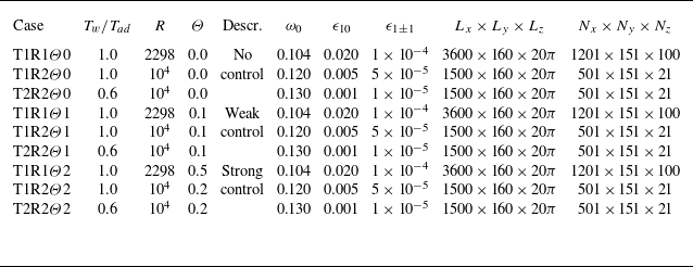
, unless otherwise specified. Nine case studies are selected, with various controlling parameters, computational domains and numbers of grid points, as illustrated in table 1. In all the cases, the fundamental spanwise wavenumber
 $\beta _0$
is set to 0.1, which was identified as corresponding to approximately the maximum growth rate of the secondary instability modes for case T1R1, as demonstrated in our previous study Song, Dong & Zhao (Reference Song, Dong and Zhao2024). Consequently, the spanwise computational domain for DNS,
 $L_z$
, is specified as
 $2\pi /\beta _0=20\pi$
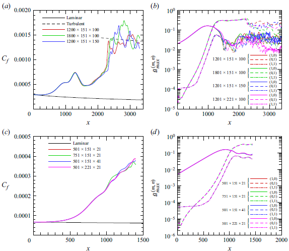
for all the cases. The resolution study for case T1R1
 $\Theta$
0 is presented in figure 19(a,b) in Appendix A, demonstrating the convergence of the numerical results until the late transition phase. The same mesh scale is utilised for cases T1R1
 $\Theta$
1 and T1R1
 $\Theta$
2. For cases with higher Reynolds numbers, specifically T1R2 and T2R2, a shorter computational domain in the streamwise direction is used, as our focus is more on the FR phase. This flow field necessitates a sparser mesh scale, with the resolution study provided in figure 19(c,d) in Appendix A.
Controlling parameters for case studies, where
 $\beta _0=0.1$
.

Streamwise velocity (a) and temperature (b) of the compressible Blasius solution at
 $x=0$
for cases T1 and T2.

The velocity and temperature profiles of the base flow at the inlet of computational domain for cases T1 and T2, obtained by the compressible Blasius solution, are displayed in figure 2. As the wall temperature decreases, the boundary-layer thickness reduces, while the wall velocity shear and temperature gradient increase.
3.2. Linear stability theory
In figure 3, we calculate the growth rates
 $-\alpha _i$
of the 2-D Mack instabilities obtained by numerically solving the O–S equations with varying frequencies. Panels (a) and (b) illustrate the results for cases T1 and T2, respectively. In each panel, two distinct unstable regions are identified, corresponding to the Mack first and second modes (Mack Reference Mack1975), with the second mode exhibiting stronger instability. Results are presented for three Reynolds numbers:
 $R=2298$
,
 $1\times 10^4$
and
 $\infty$
, with
 $R=\infty$
representing the solutions of the Rayleigh equations. The growth rate generally increases with the Reynolds number, indicating the inviscid nature of the 2-D Mack modes.
Dependence on the frequency
 $\omega$
of the growth rate
 $-\alpha _i$
of 2-D modes at
 $x=0$
for (a) case T1 and (b) case T2.

The accumulated amplitude of each instability mode can be quantified by an
 $N$
factor according to the LST, defined by
 \begin{equation} N(x)=\int _0^x-\alpha _i(\bar {x}) {\rm d}\bar {x}. \end{equation}
Figure 4 illustrates the streamwise evolution of the
 $N$
factors for 2-D Mack modes with representative frequencies in the second-mode frequency band. Analysis reveals that the most amplified second modes in the interval
 $x\in [0,1500]$
correspond to frequencies
 $\omega =0.104$
for case T1R1,
 $\omega =0.120$
for case T1R2 and
 $\omega =0.130$
for case T2R2. These frequencies are subsequently adopted as the fundamental frequencies
 $\omega _0$
in the DNS calculations, as listed in table 1. Figure 5 further plots the perturbation velocity and temperature profiles of the inflow perturbations for the DNS. For the 2-D mode,
 $\hat {\Phi }_{10}$
, the perturbation velocity exhibits a peak within the bulk boundary layer (
 $y\approx 5$
), while the perturbation temperature reaches its maximum at the critical layer near the outer edge of the boundary layer. In contrast, for the 3-D mode,
 $\hat {\Phi }_{11}$
, both the velocity and temperature perturbations display a notable peak at the critical layer.
Streamwise evolution of
 $N$
factors of 2-D second modes for (a) case T1R1, (b) case T1R2 and (c) case T2R2.

Norms of the eigenfunctions for modes
 $(1,0)$
and
 $(1,1)$
obtained by LST for cases T1R1, T1R2 and T2R2 at
 $x=0$
. The profiles are normalised by the maximum of the streamwise velocity perturbation.

3.3. Direct numerical simulation studies of the effect of surface heating on transition
For cases with
 $T_w/T_{ad}=1$
and
 $R=2298$
(also known as case T1R1), we introduce the same inflow perturbations as outlined in table 1, and simulate the transition process by imposing various intensities of surface heating. The transition process can be visualised clearly by the surface friction coefficient, defined by
 $C_f=2{R}^{-1}({\underline {\mu }}{\partial \underline {u}}/{\partial y})_{y=0}$
. Here,
 $\underline {u}$
and
 $\underline {\mu }$
represent the temporal and spanwise average of the streamwise velocity and the dynamic viscosity, respectively. The temporal averaging is performed over ten periods of the fundamental mode (
 $20\pi /\omega _0$
) to ensure statistical convergence.
Streamwise evolution of the
 $C_f$
curves obtained by DNS for cases T1R1
 $\Theta$
0 (no control), T1R1
 $\Theta$
1 (weak control) and T1R1
 $\Theta$
2 (strong control), with the dashed and dash-dotted curves denoting the empirical curves for the laminar and turbulent states, respectively.

Figure 6 compares the streamwise evolution of the
 $C_f$
curves among cases T1R1
 $\Theta$
0, T1R1
 $\Theta$
1 and T1R1
 $\Theta$
2. For the uncontrolled case T1R1
 $\Theta$
0, the
 $C_f$
curve undergoes a notable deviation from the laminar state from
 $x\approx 150$
, and increases rapidly until
 $x\approx 1300$
. Following this, there is a decrease within the range
 $x\in [1300,1500]$
, after which the
 $C_f$
curve starts to rise again, eventually causing breakdown of the laminar state and reaching the turbulent state as predicted by the empirical formula in White (Reference White2006). The two sharp increases of
 $C_f$
appears as a representative feature of FR, as depicted in Hader & Fasel (Reference Hader and Fasel2017, Reference Hader and Fasel2019), Zhu et al. (Reference Zhu, Chen, Wu, Chen, Lee and Gad-el Hak2018) and Unnikrishnan & Gaitonde (Reference Unnikrishnan and Gaitonde2020). Imposing heating segments from
 $x=500$
, as shown by the curves for cases T1R1
 $\Theta$
1 and T1R1
 $\Theta$
2, the second increase of
 $C_f$
is postponed, with a more pronounced effect observed for a higher
 $\Theta$
value. These scenarios indicate an effective control of transition by surface heating.
Visualisation of flow structures using isosurface of
 $Q$
-criterion (
 $Q=5\times 10^{-4})$
obtained from the DNS for cases T1R1
 $\Theta$
0 (no control), T1R1
 $\Theta$
1 (weak control) and T1R1
 $\Theta$
2 (strong control). The isosurface is coloured by the streamwise velocity magnitude.

The flow structures based on the
 $Q$
-criterion for the three cases are compared in figure 7. Initially, 2-D planar structures predominate, followed by a spanwise modulation due to the presence of oblique secondary waves that amplify successively. In the later stages, the interaction between the dominant planar wave and finite-amplitude oblique waves leads to the formation of
 $\varLambda$
-vortices. Then, the tips of the
 $\varLambda$
-vortices lift up from the surface while the legs remain close to the wall, ultimately breaking down into smaller scales as the flow begins to transition to turbulence. As the intensity of surface heating increases, the emergence of the
 $\varLambda$
-vortices and smaller-scale structures is delayed, particularly evident in case T1R1
 $\Theta 2$
, illustrating the transition-delaying effect of surface heating.
In figure 8, we further compare the contours of the time-averaged streamwise velocity among the three cases, where low- and high-speed streaks are clearly evident in the late nonlinear phase. As the intensity of surface heating increases, the emergence location of the streaks progressively shifts downstream, accompanied by a decrease in their intensity. This observation suggests that surface heating has a suppressive effect on the fundamental frequency resonance mechanism.
Contours of time-averaged streamwise velocity
 $\bar {u}$
in
 $x$
–
 $z$
planes at
 $y=8$
for (a) case T1R1
 $\Theta$
0 (no control), (b) case T1R1
 $\Theta$
1 (weak control) and (c) case T1R1
 $\Theta$
2 (strong control).

Streamwise evolution of the amplitude of (a)
 $\tilde {u}_{max}^{(1,0)}$
, (b)
 $\tilde {u}_{max}^{(0,0)}$
, (c)
 $\tilde {u}_{max}^{(0,1)}$
and (d)
 $\tilde {u}_{max}^{(1,1)}$
for cases T1R1
 $\Theta$
0 (no control), T1R1
 $\Theta$
1 (weak control) and T1R1
 $\Theta$
2 (strong control) obtained by DNS.

Performing the Fourier transform of the instantaneous flow field,
 \begin{equation} {\boldsymbol{\Phi }}(x,y,z,t)=\sum _{m,n=-\infty }^{\infty }\tilde {\boldsymbol{\Phi }}_{mn}(x,y)\exp \left [i(n\beta _0 z-m\omega _0 t)\right ], \end{equation}
we are able to trace the amplitude of each Fourier component
 \begin{equation} \tilde {u}_{max}^{(m,n)}(x)=\left \{ \begin{aligned} &{\max}_y\left |\tilde {u}_{mn}(x,y)+\textrm{c.c.}\right |,\quad m\neq 0\lor n\neq 0, \\ &{\max}_y\left |\tilde {u}_{mn}(x,y)-U_B(x,y)\right |,\quad m=0\land n=0. \end{aligned} \right . \end{equation}
In figure 9, we plot the streamwise evolution of
 $\tilde {u}_{max}^{(m,n)}$
for the fundamental perturbation (1,0), the mean-flow distortion (0,0), the streak mode (0,1) and the oblique mode (1,1), where the grey area indicates the region of the surface heating segment. In the uncontrolled case, the fundamental mode (1,0), shown in panel (a), evolves in the linear regime during the early laminar phase, aligning with the LST predictions denoted by the circles. This alignment persists until approximately
 $x\approx 800$
. After that, the (1,0) mode exhibits a plateau until
 $x\approx 1300$
, followed by a mild decrease leading to oscillations in the turbulent phase. The red curve in panel (b) displays the evolution of the mean-flow distortion (0,0), becoming evident from
 $x\approx 500$
, which corresponds to the early increase of the
 $C_f$
curve in figure 6. This mean-flow distortion is primarily induced by the self-interaction of the finite-amplitude mode (1,0). The subsequent local dampening of the
 $C_f$
curve is closely related to the decrease of the amplitude of the fundamental mode (1,0) in the region
 $x\in [1300,1500]$
, further reinforcing the dominant role of the (1,0) mode in the early nonlinear stage.
Similar to the fundamental mode (1,0), the oblique mode (1,1), shown in panel (d), initially evolves in the linear regime, but with a shorter region (
 $x\approx 500$
). Beyond this location, the mode (1,1) grows at a significantly higher rate than the LST prediction, indicating a secondary instability arising from the FR mechanism, which was revealed through asymptotic analysis by Song et al. (Reference Song, Dong and Zhao2024). Remarkably, in this region, the streak mode (0,1), illustrated in panel (c), amplifies at almost the same rate as the mode (1,1), but with a much greater amplitude compared with (1,1). This concurrent growth of the streak mode highlights its importance in the dynamics of the perturbation field during this transitional phase.
When heating segments are introduced from
 $x=500$
, the mode (1,0), shown in figure 9(a), exhibits a local kink with a slightly enhanced amplitude, indicating a local scattering effect as theoretical studied by Zhao & Dong (Reference Zhao and Dong2022). In contrast, the growth rates of modes (0,1) and (1,1) during the FR process are suppressed, with a more profound suppression observed in cases with stronger control. Although not shown, other Fourier modes that experience rapid growth during this nonlinear phase are also suppressed. The suppression of the FR process results in a more gradual decay of mode (1,0) in the range of
 $x\in [1200,1800]$
and also delays the rapid production of the mean-flow distortion in the late transition phase. This interaction underscores the complex relationship between the surface heating and the secondary instability modes within the flow dynamics.
3.4. Analysis of the secondary instability modes
To predict the growth rate
 $\sigma$
from the instability point of view, we perform a SIA following Chen, Zhu & Lee (Reference Chen, Zhu and Lee2017) and Song et al. (Reference Song, Dong and Zhao2024). The base flow at a given position
 $\bar x$
is considered as a superposition of a steady base flow and a series of quasi-saturated travelling waves. In a moving frame, the base flow
 $\breve {\boldsymbol{\Phi }}_{\!B}$
is expressed as
 \begin{equation} \breve {\boldsymbol{\Phi }}_{\!B}=\left (\rho _B,U_B-c_r,0,0,T_B\right )(y;\bar x)+\sum _{m=-M_w}^{M_w}\breve {\Phi }_{m0}(y;\bar x)\exp (\mathop {\textrm {i}}\nolimits m \alpha _0\tilde {x})+ \cdots , \end{equation}
where
 $\alpha _0=\mbox{Re}(\alpha )$
and
 $c_r=\omega _0/\alpha _0$
denote the real part of the wavenumber and phase speed of the fundamental mode, respectively,
 $\tilde {x}=x-c_r t$
is the Galilean transformed coordinate and
 $M_w$
denotes the order of the Fourier-series truncation. In this paper, we choose
 $M_w=3$
. Given that the fundamental mode almost reaches the saturation state, its growth rate is considered to be sufficiently small, such that
 $\alpha _0\in \mathbb R$
is a good approximation. Since the base flow
 $\breve {\boldsymbol{\Phi }}_{\!B}$
evolves in a length scale much greater than the fundamental-mode wavelength
 $2\pi /\alpha _0$
, its non-parallelism is neglected.
Following a standard Floquet analysis, the secondary instability modes
 $\tilde {\boldsymbol{\Phi }}_w$
supported by the periodic base flow
 $\breve {\boldsymbol{\Phi }}_{\!B}$
are expressed as
 \begin{equation} \begin{gathered} \tilde {\boldsymbol{\Phi }}_w=\epsilon _w \breve {\boldsymbol{\Phi }}_w(\tilde {x},y)\exp \left [ \sigma (\tilde {x}+c_r t)+\mathop {\textrm {i}}\nolimits \bar \beta z+\mathop {\textrm {i}}\nolimits \sigma _d\tilde {x}\right ]+\textrm{c.c.,} \end{gathered} \end{equation}
where
 $\sigma$
represents the growth rate,
 $\bar \beta$
is the spanwise wavenumber,
 $\sigma _d$
is the detuning parameter and
 $\epsilon _w\ll 1$
characterises the amplitude. For FR,
 $\sigma _d=0$
. Substituting (3.4) and (3.5) into (2.4) and neglecting terms of
 $O(\epsilon _w^2)$
, we obtain a linear homogeneous system
 \begin{equation} \big(\boldsymbol{H}_0+\sigma \boldsymbol{H}_1+\sigma ^2\boldsymbol{H}_2\big )\breve {\boldsymbol{\Phi }}_w (\tilde {x},y)=0, \end{equation}
where
 $\boldsymbol{H}_0$
,
 $\boldsymbol{H}_1$
and
 $\boldsymbol{H}_2$
are all
 $5\times 5$
-order matrices, whose non-zero elements can be found in Song et al. (Reference Song, Dong and Zhao2024). The wall-normal boundary conditions are prescribed as
 \begin{equation} \left . \begin{gathered} \big(\breve {u}_w,\breve {v}_w,\breve {w}_w,\breve {T}_w\big )=0,\quad \mbox{at} \ y=0,\\ \big(\breve {\rho }_w,\breve {u}_w,\breve {v}_w,\breve {w}_w,\breve {T}_w\big )\rightarrow 0,\quad \mbox{as}\ y\rightarrow \infty . \end{gathered} \right \} \end{equation}
The linear system (3.6) with homogeneous boundary conditions constitutes an eigenvalue problem with growth rate
 $\sigma$
appearing as the eigenvalue. A pseudo-spectral method is employed to solve this problem, with an expansion in the streamwise direction imposed
 \begin{equation} \breve {\boldsymbol{\Phi }}_w(\tilde {x},y)=\sum _{n=-N_w}^{N_w}\hat {\boldsymbol{\Phi }}_{w,n}\exp (\mathop {\textrm {i}}\nolimits n\alpha _0 \tilde x), \end{equation}
where
 $N_w$
is the order of Fourier-series truncation that is taken to be 6 in this paper. The component
 $\hat {\boldsymbol{\Phi }}_{w,0}$
represents the streak mode, whilst
 $\hat {\boldsymbol{\Phi }}_{w,n}$
with
 $n\neq 0$
denotes the travelling mode. The numerical code for SIA has been previously applied to studies such as Song et al. (Reference Song, Zhao and Dong2023) and Song et al. (Reference Song, Dong and Zhao2024).
As revealed by the asymptotic analysis in Song et al. (Reference Song, Dong and Zhao2024), the growth rate of the secondary instability modes (0,1) and (1,1),
 $\sigma :={\rm d}_x[\log (\tilde {u}_{max}^{(0,1)})]\approx {\rm d}_x[\log (\tilde {u}_{max}^{(1,1)})]$
, shows a distinguished scaling relation with the amplitude of the fundamental mode
 $\tilde {u}_{max}^{(1,0)}$
. For convenience, we denote
 $\bar \epsilon _{10}(x):=\tilde {u}_{max}^{(1,0)}(x)/2$
, and introduce a rescaled growth rate at a give position
 $\bar {\sigma }=\sigma /\bar {\epsilon }_{10}$
. The streamwise evolution of
 $\bar \sigma$
around the earlier nonlinear phase is depicted in figure 10. An interval where the growth rates of the secondary modes (0,1) and (1,1) agree is evident for each case. This can be accurately predicted by SIA, as illustrated by the circles. Remarkably, the surface heating leads to a reduction of the rescaled growth rate
 $\bar \sigma$
, with the case for a stronger heating producing a more profound stabilising effect.
Comparison of the rescaled growth rates of the secondary instability modes
 $\bar {\sigma }$
obtained by DNS and SIA for cases T1R1
 $\Theta$
0–T1R1
 $\Theta$
2.

Streamwise evolution of the amplitude of representative Fourier components
 $\tilde {u}_{max}^{(m,n)}$
obtained by DNS. (a) cases T1R2
 $\Theta$
0–T1R2
 $\Theta$
2; (b) cases T2R2
 $\Theta$
0–T2R2
 $\Theta$
2. The horizontal dashed lines denote the locations where
 $\bar \epsilon _{10}=0.065$
.

In figure 11, we present the amplitude evolution of Fourier components obtained by DNS for cases T1R2 and T2R2 with various surface heating intensities. Consistent with the findings of lower-Reynolds-number cases, the Fourier components (0,1) and (1,1) experience significant amplification during the nonlinear phase due to the resonance mechanism, with this growth rate being stabilised by surface heating. Notably, surface heating has a limited effect on the evolution of the fundamental modes for a given wall temperature and Reynolds number. For the subsequent SIA, we choose a streamwise location where the amplitude of the fundamental mode
 $\bar \epsilon _{10}=0.065$
for demonstration, as indicated by the horizontal dashed lines. It is important to note that, as long as this location is within the FR region, the subsequent analysis will not be sensitive to the choice of
 $\bar \epsilon _{10}$
. In figure 12, we plot the rescaled growth rate
 $\bar \sigma$
at the selected location as a function of the rescaled heating intensity
 $\Theta T_w/T_{ad}$
. Although there are some quantitative discrepancies between the DNS calculations and the SIA predictions, both display a consistent trend:
 $\bar \sigma$
decreases almost linearly with increasing
 $\Theta$
when the latter is not large. This suggests that the correction of
 $\bar \sigma$
induced by surface heating may be predicted using a perturbation technique, as will be discussed in § 4.
Variation of rescaled growth rate
 $\bar {\sigma }$
with the intensity of surface heating
 $\Theta$
at fixed fundamental-mode amplitude
 $\bar \epsilon _{10}=0.065$
for (a) case T1R2 and (b) T2R2.

Direct numerical simulation calculations of the Fourier components
 $\tilde {u}_{max}^{(m,n)}$
for case T1R2 with
 $\omega _0=0.11$
(a) and
 $\omega _0=0.13$
(b). The green curves, labelled by ‘strong control’, indicate
 $\Theta =0.5$
. In (b), the heating segment is implemented from
 $x_0=400$
.

To further validate the robustness of this control strategy, we conduct DNS calculations for case T1R2 using different fundamental frequencies
 $\omega _0$
and compare the results between the uncontrolled case (red curves) and the strongly controlled case (green curves;
 $\Theta =0.5$
). The streamwise evolution of the Fourier components is displayed in figure 13. As revealed by Zhao & Dong (Reference Zhao and Dong2022), local surface heating destabilises the Mack modes with frequencies below the critical frequency (approximately equal to the frequency of the most unstable second mode), while stabilising those with higher frequencies. This observation aligns with our results, where the surface heating enhances the fundamental mode (1,0) for
 $\omega _0=0.11$
(panel a) and suppresses (1,0) for
 $\omega _0=0.13$
(panel b). Furthermore, both panels demonstrate a notable stabilising effect on the secondary modes (0,1) and (1,1). Additionally, in panel (b), we position the heating segment at a different streamwise location,
 $x_0=400$
, which is upstream of the FR range. This adjustment does not affect the effectiveness of the control strategy.
4. Asymptotic analysis for impact of surface heating on fundamental resonance
4.1. Asymptotic model for fundamental resonance without control
To reveal the mechanism ensuring the suppression of FR by surface heating, we construct an asymptotic model that quantifies the correction of the growth rate of the streak and oblique travelling modes. Our previous work (Song et al. Reference Song, Dong and Zhao2024) has revealed that the FR is in principle a triad resonance system operating among a streak mode and a pair of oblique travelling modes, with the saturated planar fundamental mode injecting energy to this system. Accordingly, the flow field can be expressed as
 \begin{align} {\boldsymbol{\Phi }}(x,y,z,t)&= \displaystyle \bar {\boldsymbol{\Phi }}(y;x)+ \bar {\epsilon }_{10}\tilde {\boldsymbol{\Phi }}_{10}(y;x)\;{\mathop {\textrm {e}}\nolimits }^{\mathop {\textrm {i}}\nolimits (\int {\alpha _{10}} {\rm d}x-\omega _0 t)} \nonumber\\ &\quad \displaystyle +{\mathop {\textrm {e}}\nolimits }^{\sigma x}\left [\bar \epsilon _{01}\tilde {\boldsymbol{\Phi }}_{01}(y;x)\;{\mathop {\textrm {e}}\nolimits }^{\mathop {\textrm {i}}\nolimits \beta _0z}+\bar {\epsilon }_{11}\tilde {\boldsymbol{\Phi }}_{11}(y;x)\;{\mathop {\textrm {e}}\nolimits }^{\mathop {\textrm {i}}\nolimits (\int \alpha _{11} {\rm d}x+\beta _0z-\omega _0t)}\right .\nonumber \\ &\quad\left . +\, \bar {\epsilon }_{1-1}\tilde {\boldsymbol{\Phi }}_{1-1}(y;x)\;{\mathop {\textrm {e}}\nolimits }^{\mathop {\textrm {i}}\nolimits (\int \alpha _{11} {\rm d}x-\beta _0z-\omega _0t)}+ \cdots \right ]+\textrm{c.c.,} \end{align}
where
 $\alpha _{10}$
denotes the wavenumber of the fundamental mode, which is almost real,
 $\alpha _{11}$
denotes the common wavenumber of the oblique modes,
 $\bar {\epsilon }_{mn}\ll 1$
denotes the amplitude of the Fourier component
 $(m,n)$
and the subscripts
 $10$
,
 $01$
and
 $11$
(or
 $1{-}1$
) denote the fundamental mode, the streak mode and the 3-D travelling mode, respectively. Since the fundamental mode originates from the Mack instability, we consider the fundamental frequency
 $\omega _0$
and spanwise wavenumber
 $\beta _0$
, along with the wavenumbers
 $\alpha _{10}$
and
 $\alpha _{11}$
, to be
 $O(1)$
. Given that the growth rates of the oblique perturbations are encapsulated in
 ${\mathop {\textrm {e}}\nolimits }^{\sigma x}$
, we take
 $\alpha _{11}$
to be real, which we will denote as
 $\alpha _0$
to align with the wavenumber of the SIA in § 3. Following the SIA, we choose
 $\alpha _0=\mbox{Re}(\alpha _{10})$
. The amplitudes of the representative Fourier components are given by
 $\bar {\epsilon }_{10}\gg \bar {\epsilon }_{01}\gg \bar {\epsilon }_{11}$
, and specifically, we let
 \begin{equation} \bar {\epsilon }_{11}=\bar {\epsilon }_{10}\bar {\epsilon }_{01}. \end{equation}
There could be various approaches to determine the mean flow
 $\bar {\boldsymbol{\Phi }}$
, and the most direct way is to extract it from the DNS data. However, DNS is too costly. Given that the Blasius base flow is known, we can employ the nonlinear parabolised stability equation (NPSE) to calculate the mean-flow distortion induced by the nonlinear feedback of the fundamental mode. The introduction of NPSE can be found in Bertolotti, Herbert & Spalart (Reference Bertolotti, Herbert and Spalart1992)and Chang & Malik (Reference Chang and Malik1994), and it has been used extensively in our previous studies (Zhao et al. Reference Zhao, Zhang, Liu and Luo2016; Song et al. Reference Song, Zhao and Dong2023).
In the bulk of the boundary layer, the fundamental mode is governed by the Rayleigh equation
 \begin{equation} {\mathcal L}_R({\alpha _{10}},\beta _0,\omega _0)\tilde {\boldsymbol{\varphi }}_{10}=0,\quad \tilde {\boldsymbol{\varphi }}_{10}=(\tilde v_{10},\tilde p_{10})^T; \end{equation}
the mathematical details can be found in Dong et al. (Reference Dong, Liu and Wu2020). Considering the leading-order boundary conditions
 \begin{equation} \tilde v_{10}(0)=0, \quad \tilde p_{10}(\infty )\to 0, \end{equation}
this system forms an eigenvalue problem, with
 $\alpha _{10}$
appearing as the eigenvalue. In the saturation phase, the imaginary part of
 $\alpha _{10}$
is relatively small, which often leads to the emergence of a critical layer at
 $\bar {U}=\omega _0/\alpha _{0}$
. This critical layer can pose challenges to the numerical process. To address this issue, we modify the integrating path in complex space to circumvent the critical point. This approach has been successfully utilised in our previous studies (Dong et al. Reference Dong, Liu and Wu2020; Song et al. Reference Song, Dong and Zhao2024), allowing for more stable and accurate numerical computations despite the presence of critical layers.
Remarkably, at a moderate Reynolds number, the predictions of the Rayleigh equation on the growth rate always yield a certain error, and an improvement of the accuracy can be achieved by taking into account the impact of the viscous Stokes layer in the
 $O(R^{-1/2})$
vicinity of the wall. According to Dong et al. (Reference Dong, Liu and Wu2020), the improved Rayleigh system is also governed by (4.3), but with the wall boundary condition modified as
 \begin{equation} \tilde v_{10}=-C_w^{1/2}\left [\frac {\mathop {\textrm {i}}\nolimits (\gamma -1)\omega _0 M^2}{(-\mathop {\textrm {i}}\nolimits \omega _0 Pr)^{1/2}}+\frac {{\alpha _{10}}^2\bar T_w}{(-\mathop {\textrm {i}}\nolimits \omega _0)^{3/2}}\right ]R^{-1/2}\tilde p_{10}(0), \end{equation}
where
 $-\mathop {\textrm {i}}\nolimits \equiv {\mathop {\textrm {e}}\nolimits }^{3\pi /2}$
,
 $\bar T_w=\bar T|_{y=0}$
and
 $C_w=\mu (\bar T_w)\bar T_w$
. The improved boundary condition includes the impact of the Reynolds number, and it is evident that, as
 $R\to \infty$
, the right-hand side of (4.5) approaches zero. Numerical predictions based on the improved Rayleigh equation achieves an accurate prediction of the Mack-mode growth rate even when
 $R$
is a few thousands.
The perturbation profiles of the streak mode are more complex, as the roll structure, represented by
 $\tilde v_{01}$
and
 $\tilde w_{01}$
, pertains to an
 $O(\bar \epsilon _{10})$
magnitude of the streak structure, represented by
 $\tilde u_{01}$
. Therefore, we rescale the perturbation by introducing
 \begin{equation} \big(\tilde {u}_{01},\tilde {v}_{01},\tilde {w}_{01},\tilde {p}_{01},\tilde {\rho }_{01},\tilde {T}_{01}\big )=\big (\breve {u}_{01},\bar {\epsilon }_{10}\breve {v}_{01},\bar {\epsilon }_{10}\breve {w}_{01},\bar {\epsilon }_{10}^2\breve {p}_{01},\breve {\rho }_{01},\breve {T}_{01}\big ). \end{equation}
The combined system governing the streak mode and the oblique modes in the bulk boundary layer can be expressed in terms of a sixth-order linear differential system
 \begin{equation} {\mathcal L}_c(\alpha _0,\beta _0,\omega _0,\bar \sigma )\tilde {\boldsymbol{\varphi }}:= \left (\frac {\rm d}{{\rm d}y}-\boldsymbol{A}\right )\tilde {\boldsymbol{\varphi }}=0, \end{equation}
where
 $\tilde {\boldsymbol{\varphi }}= (\tilde {v}_{11},\tilde {p}_{11},\tilde {v}_{1-1},\tilde {p}_{1-1},\breve {v}_{01},\breve {p}_{01} )^T$
, and the coefficient matrix
 $\boldsymbol{A}$
can be found in Song et al. (Reference Song, Dong and Zhao2024). The non-penetration and attenuation conditions are imposed at the lower boundary
 \begin{equation} \tilde {v}_{11}(0) = \tilde {v}_{1-1}(0) = \breve {v}_{01}(0) = 0;\quad (\tilde {p}_{11}, \tilde {p}_{1-1}, \breve {p}_{01})_{y\to \infty } \to 0. \end{equation}
This homogeneous system constitutes an eigenvalue problem, with the rescaled growth rate
 $\bar \sigma$
being the eigenvalue.
Again, for a more accurate prediction, we need to consider a wall layer in the
 $O(\bar \epsilon _{10}R)^{-1/3}$
vicinity of the wall. Following Song et al. (Reference Song, Dong and Zhao2024), we obtain the improved wall boundary condition for (4.7)
 \begin{equation} \breve {v}_{01}(0)=\epsilon \ln \epsilon V_{\infty },\quad \tilde {v}_{11}(0)=\tilde {v}_{1-1}(0)=\epsilon \ln \epsilon V_{1\infty }, \end{equation}
where
 $\epsilon =(\bar {\epsilon }_{10}R)^{-1/3}$
and
 \begin{align}&\qquad\qquad\qquad\qquad\qquad\quad V_{\infty }=-\frac {0.7764\mathop {\textrm {i}}\nolimits \beta _0}{(\lambda \bar {\sigma })^{4/3}}\left (\hat {A}_3-\frac {\lambda _T\hat {A}_2}{\bar T_w}\right ), \end{align}
 \begin{align}& V_{1\infty }=\frac {\alpha _0\beta _0 C_w^{1/3}\tilde {p}_{10}(0)}{\bar {\sigma }^{7/3}\lambda ^{4/3}}\left [\! C_1 \left (\!M^2+\frac {\alpha ^2}{\omega ^2}\right )+C_2\left (\!M^2-\frac {\alpha _0^2}{\omega _0^2}\!\right )+C_3\frac {\lambda _T\alpha _0}{\lambda \omega _0}\!\right ]\left (\!\hat {A}_3-\frac {\lambda _T\hat {A}_2}{\bar T_w}\!\right )\!, \end{align}
with
 $\lambda =\bar {U}_y(0)$
,
 $\lambda _T=\bar {T}_y(0)$
,
 $C_w=\mu _w T_w$
,
 $C_1=-0.8869$
,
 $C_2=0.1139$
,
 $C_3=-1.0221$
and
 \begin{align}& \hat {A}_2=-2\mathop {\textrm {i}}\nolimits \mbox{Im}\big[\!\lambda _{v10}^\dagger \tilde {w}_{11}(0)\!\big ], \hat {A}_3=-2\mathop {\textrm {i}}\nolimits \mbox{Im}\left [\!\lambda _{v10}^\dagger \tilde {w}_{11,y}(0)+\left (\!{\lambda }_{v10}^\dagger -\frac {\lambda _T\lambda _{v10}^\dagger }{\bar T_w}\!\right )\!\right ], \end{align}
 \begin{align}&\qquad\qquad\qquad\qquad\quad \lambda _v=\tilde {v}_{10,y}(0),\quad \lambda _v^\dagger =\tilde {v}_{10,yy}(0). \end{align}
4.2. Impact of surface heating on FR
Here, we assume the intensity of surface heating
 $\Theta$
to be much smaller than unity, then, the mean flow can be expanded as
 \begin{equation} \bar {\boldsymbol{\Phi }}+\Theta \tilde {\boldsymbol{\Phi }}_{1}+O(\Theta ^2), \end{equation}
where
 $\tilde {\boldsymbol{\Phi }}_{1}$
denotes the mean-flow distortion induced by the scattering effect of the surface heating segment, which can be obtained by the HLNS approach. It has been confirmed in Zhao & Dong (Reference Zhao and Dong2022) and Zhao, He & Dong (Reference Zhao, He and Dong2023) that the HLNS calculations of the mean-flow distortion induced by heating source can be sufficiently accurate even when
 $\Theta$
is
 $O(0.1)$
.
Accordingly, the perturbations of the fundamental mode, the streak mode and oblique modes are expanded as
 \begin{align} &\qquad\qquad\tilde {\boldsymbol{\Phi }}_{10}{\mathop {\textrm {e}}\nolimits }^{\mathop {\textrm {i}}\nolimits (\int ({\alpha _{10}+\Theta {\alpha }_1}) {\rm d}x-\omega _0 t)}+\Theta \tilde {\boldsymbol{\Phi }}_{101}{\mathop {\textrm {e}}\nolimits }^{\mathop {\textrm {i}}\nolimits (\int \alpha _{10} {\rm d}x-\omega _0 t)}+O(\Theta ^2), \end{align}
 \begin{align} &\qquad\qquad\qquad\tilde {\boldsymbol{\Phi }}_{01}{\mathop {\textrm {e}}\nolimits }^{\mathop {\textrm {i}}\nolimits \beta _0z}{\mathop {\textrm {e}}\nolimits }^{(\sigma +\Theta \sigma _1)x}+\Theta \tilde {\boldsymbol{\Phi }}_{011}{\mathop {\textrm {e}}\nolimits }^{\mathop {\textrm {i}}\nolimits \beta _0z}{\mathop {\textrm {e}}\nolimits }^{\sigma x}+O(\Theta ^2), \end{align}
 \begin{align} &\tilde {\boldsymbol{\Phi }}_{1\pm 1}{\mathop {\textrm {e}}\nolimits }^{\mathop {\textrm {i}}\nolimits (\int ( \alpha _0+\Theta \alpha _1) {\rm d}x\pm \beta _0z-\omega _0 t)}{\mathop {\textrm {e}}\nolimits }^{(\sigma +\Theta \sigma _1)x}+\Theta \tilde {\boldsymbol{\Phi }}_{1\pm 11}{\mathop {\textrm {e}}\nolimits }^{\mathop {\textrm {i}}\nolimits (\int \alpha _0 {\rm d}x\pm \beta _0z-\omega _0 t)}{\mathop {\textrm {e}}\nolimits }^{\sigma x}+O(\Theta ^2), \end{align}
where
 $\alpha _1$
is the wavenumber correction of the fundamental mode. Here, the leading-order quantities, of
 $O(1)$
, denote the perturbations without control, while the second-order quantities, of
 $O(\Theta )$
, denote the correction induced by the surface heating. Specifically, we also rescale the quantities of the streak mode according to their magnitudes
 \begin{equation} \big(\tilde {u}_{011},\tilde {v}_{011},\tilde {w}_{011},\tilde {p}_{011},\tilde {\rho }_{011},\tilde {T}_{011}\big) \sim \big (\breve {u}_{011},\bar {\epsilon }_{10}\breve {v}_{011},\bar {\epsilon }_{10}\breve {w}_{011},\bar {\epsilon }_{10}^2\breve {p}_{011},\breve {\rho }_{011},\breve {T}_{011}\big ). \end{equation}
The governing equations of the leading-order quantities are illustrated in § 4.1. The governing equations of the second-order fundamental mode
 $\tilde {\boldsymbol{\varphi }}_{101}=(\tilde {v}_{101},\tilde {p}_{101})^T$
can be expressed in terms of inhomogeneous Rayleigh equations
 \begin{equation} \mathcal{L}_R\tilde {\varphi }_{101}=\alpha _1\boldsymbol{F}_{101}+\boldsymbol{K}_{101}\equiv \alpha _1\begin{pmatrix} F_{101,1}\\ F_{101,2} \end{pmatrix}+\begin{pmatrix} K_{101,1}\\ K_{101,2} \end{pmatrix}, \end{equation}
where
 \begin{align} F_{101,1}&=-\mathop {\textrm {i}}\nolimits \bar {U}\tilde {v}_{10}, \end{align}
 \begin{align} F_{101,2}&=-\mathop {\textrm {i}}\nolimits \alpha _{10}\tilde {u}_{1}\tilde {v}_{10}+\bar {T}\tilde {\rho }_{1}S_0\tilde {v}_{10}, \end{align}
 \begin{align} K_{101,1}&=-\mathop {\textrm {i}}\nolimits \big[-\mathop {\textrm {i}}\nolimits \alpha _{10}\tilde {p}_{10}\bar {T}/S_0+\big (M^2S_0\tilde {p}_{10} -\mathop {\textrm {i}}\nolimits \alpha _{10}\tilde {u}_{10}\big)\bar {U}/S_0+\tilde {u}_{10}\big], \end{align}
 \begin{align} K_{101,2}&=\mathop {\textrm {i}}\nolimits \alpha _{10} \tilde {u}_{1,y}\tilde {v}_{10}/S_0-\mathop {\textrm {i}}\nolimits \alpha _{10} \tilde {u}_{1}\big(-\mathop {\textrm {i}}\nolimits \alpha _{10}\tilde {u}_{10}+M^2S_0\tilde {p}_{10}\big)+S_0\tilde {\rho }_{10}\tilde {T}_{1}-\tilde {T}_{1,y}\tilde {v}_{10}/\bar {T}\notag \\ &\quad -\bar {T}\tilde {\rho }_{1}\left (\tilde {v}_{100,y}+\tilde {v}_{10}\bar {T}_{y}/\bar {T}-\mathop {\textrm {i}}\nolimits \alpha _{10}\bar {U}_{y}\tilde {v}_{10}/S_0\right )+\bar {T}\tilde {\rho }_{1,y}\tilde {v}_{10}, \end{align}
with
 $S_0=\mathop {\textrm {i}}\nolimits \alpha _{10}(\bar {U}-c)$
and
 $c=\omega _0/{\alpha _{10}}$
. The boundary conditions are
 $\tilde {v}_{101}(0)=0$
and
 $\tilde {p}_{101}(\infty )\rightarrow 0$
. The above linear system along with the boundary condition has non-trivial solutions only if the right-hand side is orthogonal to the adjoint vector
 $\tilde {\boldsymbol{\varphi }}_{101}^\ddagger$
(solvability condition), which leads to
 \begin{equation} \alpha _1=-\frac {\big \langle \tilde {\boldsymbol{\varphi }}_{101}^\ddagger ,\boldsymbol{K}_{101}\big \rangle }{\big \langle \tilde {\boldsymbol{\varphi }}_{101}^\ddagger ,\boldsymbol{F}_{101}\big \rangle },\quad \mbox{with }\big \langle \tilde {\boldsymbol{\varphi }}^\ddagger ,\tilde {\boldsymbol{\varphi }}\big \rangle \equiv \int _0^\infty \big (\tilde {\boldsymbol{\varphi }}^\ddagger \big )^T\tilde {\boldsymbol{\varphi }} {\rm d}y. \end{equation}
After obtaining the profiles of
 $\tilde v_{101}$
and
 $\tilde p_{101}$
, the perturbation profiles of
 $\tilde u_{101}$
and
 $\tilde T_{101}$
can be obtained by substituting into the original linear system. Notably, the solution
 $\tilde {\boldsymbol{\varphi }}_{101}$
cannot be uniquely determined since a complementary solution
 $\tilde {\boldsymbol{\varphi }}_{10}$
appears. Therefore, to present a fair comparison with the uncontrolled case, we introducing
 $\tilde u_{101}(y_c)=0$
for normalisation, where
 $y_c$
is the peak location of the profile
 $|\tilde u_{10}|$
.
For the coupled system governing the second-order streak mode and oblique modes,
 $\tilde {\boldsymbol{\varphi }}_1= (\tilde {v}_{111},\tilde {p}_{111},\tilde {v}_{1-11},\tilde {p}_{1-11},\breve {v}_{011},\breve {p}_{011} )$
, we can obtain a sixth-order differential system
 \begin{equation} {\mathcal L}_c\tilde {\boldsymbol{\varphi }}_1=\bar {\sigma }_1\boldsymbol{K}_1+\alpha _{1}\boldsymbol{K}_2+\boldsymbol{M}_1+\boldsymbol{M}_2, \end{equation}
where
 $\bar \sigma _1=\sigma _1/\bar \epsilon _{10}$
. Here,
 $\boldsymbol{M}_1$
and
 $\boldsymbol{M}_2$
represent the terms related to the eigenfunction correction of fundamental mode
 $\tilde {\boldsymbol{\Phi }}_{101}$
and the modification of basic flow
 $\tilde {\boldsymbol{\Phi }}_{1}$
, respectively. The components of vectors
 $\boldsymbol{K}_{1,2}$
and matrix
 $\boldsymbol{M}_{1,2}$
are illustrated in Appendix B. Again, to leading order, the boundary conditions can be expressed as
 $\tilde {v}_{111}(0) = \tilde {v}_{1-11}(0) = \breve {v}_{011}(0) = 0$
and
 $(\tilde {p}_{111}, \tilde {p}_{1-11}, \breve {p}_{011}) \to 0$
as
 $y\to \infty$
. Based on the solvability condition, we can obtain the heating-induced correction of the growth rate of the secondary instability modes
 \begin{equation} \bar {\sigma }_1=-\frac {\alpha _{1}\big \langle \tilde {\boldsymbol{\varphi }}_{1}^\ddagger ,\boldsymbol{K}_{2}\big \rangle +\big \langle \tilde {\boldsymbol{\varphi }}_{1}^\ddagger ,\boldsymbol{M}_{1}\big \rangle +\big \langle \tilde {\boldsymbol{\varphi }}_{1}^\ddagger ,\boldsymbol{M}_2\big \rangle }{\big \langle \tilde {\boldsymbol{\varphi }}_{1}^\ddagger ,\boldsymbol{K}_{1}\big \rangle }. \end{equation}
Notably, the correction of the rescaled growth rate is contributed by three factors, including the correction of the fundamental-mode wavenumber (denoted by
 $\bar \sigma _{1,CFW}$
), the correction of the fundamental-mode profile (denoted by
 $\bar \sigma _{1,CFP}$
) and the profile of the mean-flow distortion (denoted by
 $\bar \sigma _{1,MFD}$
).
5. Asymptotic predictions
5.1. Validations for cases T1R2 and T2R2
Choosing the uncontrolled cases, T1R2
 $\Theta$
0 and T2R2
 $\Theta$
0, we compare the rescaled growth rate
 $\bar \sigma$
obtained from DNS, SIA and the asymptotic theory, as shown in figures 14(a) and 14(b), respectively. For the two cases examined, the DNS calculations for the amplitudes of modes (0,1) and (1,1) show remarkable discrepancy in the upstream region; however, when the phase-locking mechanism associated with FR is active – corresponding to the intervals
 $x\in [650,1000]$
and
 $x\in [850,1100]$
for the two panels, respectively – the two growth rates agree. These growth rates are generally predicted by both the SIA and the asymptotic theories, consistent with the findings of Song et al. (Reference Song, Dong and Zhao2024). To quantify the impact of surface heating on the growth rate
 $\bar \sigma$
, we introduce a rescaled growth-rate correction, given by
 \begin{equation} \bar {\sigma }_1=\frac {\bar \sigma |_{controlled}-\bar \sigma |_{uncontrolled}}{\Theta }, \end{equation}
where the subscripts ‘controlled’ and ‘uncontrolled’ refer to cases with and without surface heating, respectively. Here, the quantity
 $\bar \sigma$
can be obtained through either DNS or SIA. The inclusion of the denominator
 $\Theta$
is motivated by the almost linear relationship observed between the variation of
 $\bar \sigma$
and
 $\Theta$
, as revealed by figure 12. This definition is consistent with the definition provided for the asymptotic theory in (4.20). Figures 14(c) and 14(d) present a comparison of the rescaled growth-rate correction
 $\bar \sigma _1$
obtained by DNS, SIA and asymptotic theory. Given that both the DNS and SIA results consider the effects of finite Reynolds numbers and finite fundamental-mode amplitudes, it is understandable that the asymptotic predictions exhibits a quantitative error. Within the FR region, all three sets of curves exhibit negative growth-rate corrections, thereby confirming the suppression effect on the secondary instability due to the introduction of surface heating. Notably, the
 $\bar \sigma _1$
values for DNS results with different heating intensities are generally maintained at a consistent level during the FR process, demonstrating overall agreement with the asymptotic predictions.
Comparison of the leading-order growth rate
 $\bar {\sigma }$
(a,b) and second-order growth rate
 $\bar {\sigma }_1$
(c,d) obtained by DNS, SIA and asymptotic predictions. Left column: case T1R2; right column: case T2R2.

Comparison of the perturbation profiles at
 $x=900$
obtained by DNS, SIA and asymptotic theory, where the profiles are normalised by the maximum value of
 $\tilde {v}_{01}$
. Top row: leading-order eigenfunctions
 $\breve v_{01}$
; bottom row: second-order eigenfunctions
 $\breve v_{011}$
. Left column: case T1R2; right column case T2R2.

By selecting a representative streamwise location within the FR region, specifically
 $x=900$
, we compare the eigenfunctions of the leading-order streak mode
 $\breve {v}_{01}$
and the second-order streak mode
 $\breve {v}_{011}$
, obtained by DNS, SIA and the asymptotic theory for cases T1R2 and T2R2, as depicted in figures 15. For the DNS and SIA results, the definition of the second-order eigenfunction is
 \begin{equation} \breve v_{011}=\frac {\breve v_{01}|_{controlled}-\breve v_{01}|_{uncontrolled}}{\Theta }. \end{equation}
The agreement among the leading-order perturbations across the three methods is excellent. While the curves for the second-order perturbations exhibit noticeable discrepancies, the overall trends remain consistent across all cases. It is understandable that the low accuracy of the asymptotic predictions near the critical layer (
 $y\approx 18$
for T1R2 and
 $y\approx 13$
for T2R2) arises from neglecting viscosity in the leading-order approximation. Moreover, the omission of viscous effects also contributes to quantitative errors in the asymptotic predictions within the near-wall sublayer.
Dependence on
 $R$
of the leading-order growth rate
 $\bar {\sigma }$
(a) and second-order growth rate
 $\bar {\sigma }_1$
(b) obtained by the SIA and asymptotic predictions for
 $T_w/T_{ad}=1$
,
 $\omega _0=0.120$
,
 $\beta _0=0.1$
and
 $\bar \epsilon _{10}R\equiv 15\,000$
.

5.2. Validation for higher Reynolds numbers
To achieve a better comparison between the numerical results and the asymptotic predictions, we evaluate cases by increasing the Reynolds number to
 $O(10^6)$
. As indicated by § 4.1, the leading-order prediction of the growth rate
 $\bar \sigma$
scales with
 $\epsilon =(\bar \epsilon _{10}R)^{-1/3}$
due to the wall-layer-induced boundary condition. Therefore, the comparison is made by varying
 $\bar \epsilon _{10}$
and
 $R$
, while keeping
 $\bar \epsilon _{10}R$
constant. Given the challenges that such high Reynolds numbers pose for DNS, we opt to use SIA calculations derived from a model base flow as the numerical results. The model base flow exhibits a streamwise wavy nature, consisting of the compressible Blasius similarity solution and a fundamental mode (1,0) with finite amplitude. The latter is obtained by solving the O–S equation (2.8). Although this base flow is artificial, its secondary instability effectively illustrates the FR at high Reynolds numbers (Song et al. Reference Song, Dong and Zhao2024).
Figures 16(a) and 16(b) present the Reynolds-number dependence of the FR growth rate
 $\bar {\sigma }$
and its correction
 $\bar {\sigma }_1$
induced by surface heating, with calculations performed for the controlling parameters selected from case T1R2. By maintaining a fixed parameter
 $\bar \epsilon _{10}R$
, the asymptotic theory yields constant predictions, towards which the SIA results exhibit gradual convergence as the Reynolds number increases. Notably, the growth-rate correction induced by surface heating maintains negative values, demonstrating its sustained suppression effect on the FR process. The validation of the theoretical framework is further substantiated through the comparison of perturbation profiles presented in figure 17, where both the SIA solutions of
 $\breve {v}_{01}$
and its modification component
 $\breve {v}_{011}$
demonstrate progressive convergence towards the asymptotic predictions with increasing Reynolds number. This consistent agreement between SIA results and asymptotic predictions in both growth rates and perturbation profiles at high
 $R$
not only validates the asymptotic analysis framework but also confirms the robustness of the surface-heating-induced suppression mechanism on FR.
Comparison of the perturbation profiles
 $\tilde {v}_{01}$
(a) and
 $\tilde {v}_{011}$
(b) obtained by SIA and asymptotic theory. Results are shown for
 $\omega _0=0.120$
,
 $\beta _0=0.1$
and
 $\bar {\epsilon }_{10}=0.015$
.

Variation of the contributing factors on the rescaled growth rate
 $\bar {\sigma }_1$
. Results are shown for
 $\omega _0=0.120$
,
 $\beta _0=0.1$
and
 $\bar {\epsilon }_{10}=0.015$
.

As revealed by (4.20), the rescaled growth-rate correction
 $\bar \sigma _1$
consists three distinct contributing factors,
 $\bar \sigma _{1,CFW}$
,
 $\bar \sigma _{1,CFP}$
and
 $\bar \sigma _{1,MFD}$
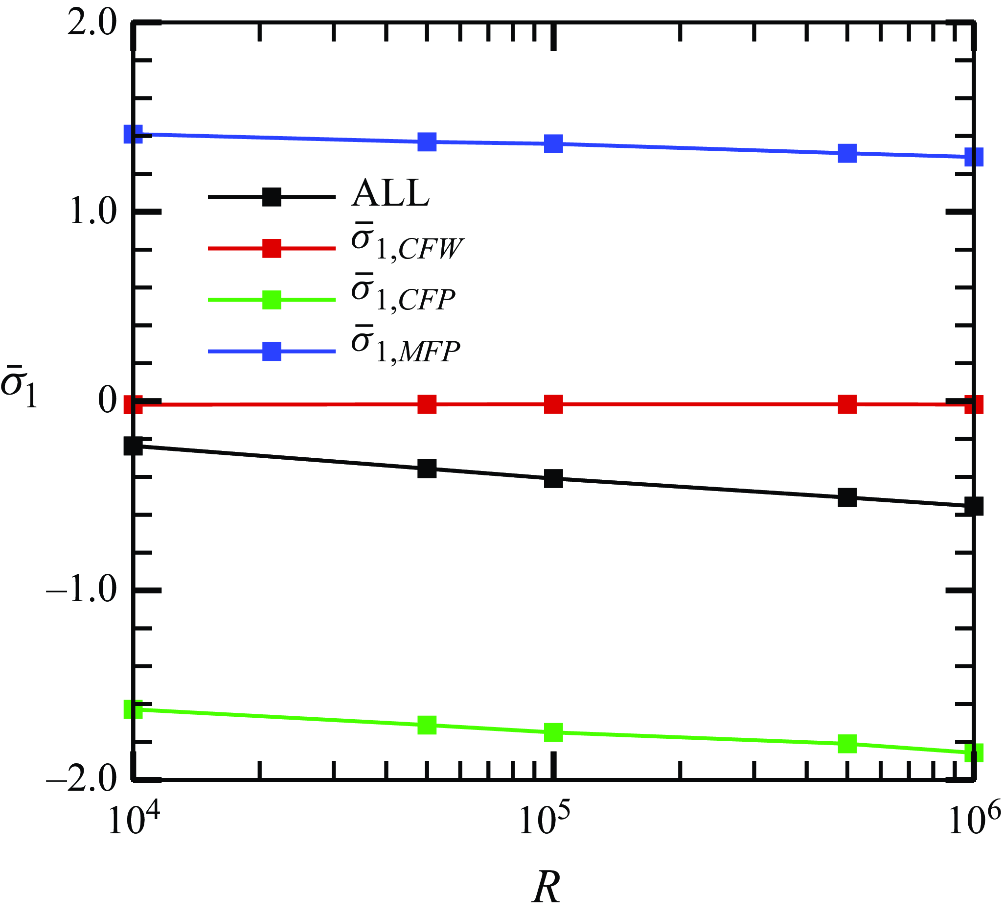
, with their contributions illustrated in figure 18. The results indicate that the latter two factors play a dominant role. Notably,
 $\bar \sigma _{1,CFP}$
serves as the primary suppression mechanism, as surface heating redistributes spatial energy within the fundamental mode to achieve suppression. In contrast,
 $\bar \sigma _{1,MFD}$
exhibits a promoting effect with its magnitude being slightly smaller than that of
 $\bar \sigma _{1,CFP}$
, resulting in an overall suppression effect. Moreover, the combined suppression effect increases with Reynolds numbers. These findings provide valuable insights for future control strategies, suggesting that approaches primarily targeting the fundamental-mode eigenfunction while avoiding significant modifications to the mean-flow structure could lead to more effective laminar flow control schemes.
6. Concluding remarks and discussion
To reduce drag and heat flux in high-speed flying vehicles, it is favourable to implement control strategies aimed at delaying boundary-layer transition to turbulence. The key principle behind these strategies is to mitigate the development of boundary-layer perturbations during the laminar phase. Numerous studies have focused on suppressing the growth of perturbations during the linear phase by introducing specific mean-flow distortions through various control strategies, such as wavy walls, blowing and suction and thermal sources. Although both numerical and experimental results have demonstrated effective delays in transition using these control strategies, linear stability analysis indicates that the impact of these strategies on Mack modes may reverse with changes in perturbation frequency (Zhao & Dong Reference Zhao and Dong2022). Consequently, implementing control strategies based on this concept requires particular caution.
In this paper, we explore an alternative concept of laminar-flow control, specifically targeting the nonlinear phase to suppress the amplification of secondary instability modes. Given that FR often occurs in quasi-2-D hypersonic boundary layers, we aim to suppress perturbations during the FR phase by introducing surface control strategies exclusively within the nonlinear phase. As a representative case study, we investigate the effects of surface heating segments in Mach 5.92 hypersonic boundary layers using DNS, SIA and asymptotic analysis.
Based on various Reynolds numbers, wall temperatures and fundamental frequencies, the DNS results consistently demonstrate that the surface heating has minimal influence on the fundamental mode (1,0), while the secondary instability modes, including the streak mode (0,1) and the oblique modes
 $(1,\pm 1)$
, are effectively suppressed. Although, at certain frequencies, the fundamental mode itself may be slightly destabilised by surface heating, the combined effect with the suppression of the secondary instability modes ensures a delay in transition, progressively postponed with increasing heating intensity
 $\Theta$
. The growth rates of the secondary instability modes obtained by DNS, along with the stabilising effect induced by surface heating, are successively predicted by SIA.
To elucidate the physical mechanisms that ensure the effectiveness and robustness of surface heating in suppressing FR, we develop a high-
 $R$
asymptotic theory based on the asymptotic FR model in Song et al. (Reference Song, Dong and Zhao2024). In this theory, the heating intensity
 $\Theta$
is assumed to be much smaller than unity, and the flow field is expanded into an uncontrolled state (leading order) and an
 $O(\Theta )$
distortion induced by surface heating (second order). Higher-order terms of
 $O(\Theta ^2)$
are neglected. The leading-order perturbations can be described by the asymptotic FR model presented in Song et al. (Reference Song, Dong and Zhao2024), where FR is characterised by a three-step loop: first, the interaction of the fundamental mode and the streak structure seeds the growth of oblique modes; second, the interaction of the fundamental mode and the oblique modes promotes the growth of roll structures; and third, the roll structure drives the growth of the streak structure through the lift-up mechanism. Thus, the streak structure, oblique modes and roll structures collectively form an eigenvalue system that aligns with the SIA concept. In cases with surface heating, the second-order perturbations are governed by an inhomogeneous linear system, with the corrections to the fundamental-mode wavenumber, the fundamental-mode profile and the mean-flow distortion induced by surface heating acting as the inhomogeneous forcing. The solvability condition helps obtain the growth-rate correction induced by surface heating, which determines the stabilising or destabilising effect on secondary instability modes. Numerical solutions for the growth-rate correction yield consistently negative values across a wide range of controlling parameters, with predictions for both growth rates and main-layer perturbation profiles showing overall agreement with SIA calculations. The asymptotic analysis further reveals that the influence of surface heating on the FR process primarily occurs through two mechanisms: corrections to the fundamental-mode profile and distortions in the mean flow. Specifically, suppression of the FR is predominantly achieved by the modification of the fundamental-mode profile, while mean-flow distortion has a comparatively mild promoting effect on this process.
This study provides compelling evidence for delaying boundary-layer transition based on the concept of controlling perturbation amplification in the nonlinear phase. It is important to note that this control strategy is not limited to surface heating; other methods such as wavy walls or suction slots could achieve similar effects on the FR if implemented during the nonlinear phase, which requires further investigations. The advantage of this approach lies in the robustness of the secondary instability mode suppression across fundamental frequencies within the second-mode frequency band, in stark contrast to the control concepts that rely on the linear evolution of Mack modes, which exhibit an opposing effect for frequencies above or below the critical frequency around the most unstable frequency of the second mode (Zhao & Dong Reference Zhao and Dong2022). Therefore, delaying transition by controlling perturbation evolution in the nonlinear phase presents a promising concept for the aerodynamic design of hypersonic vehicles.
It is important to note that, while the proposed method effectively suppresses perturbation growth during the nonlinear phase, the optimal streamwise positioning of the heating source requires further investigation. If the control is placed too early, the local heating may alter the linear growth behaviour and potentially degrade control performance. Conversely, if it is introduced too late, the secondary instability may have already been significantly amplified, reducing the effectiveness of the nonlinear suppression mechanism. This positioning is also influenced by the local receptivity and scattering effects that arise at the beginning of the control panel. Additionally, a hybrid strategy that integrates control panels during both the linear and nonlinear phases may be a promising approach. Therefore, future work will focus on optimising the placement of the heating source and assessing its sensitivity to these factors.
Funding
The work is supported by National Science Foundation of China (grant nos. 92371104, U20B2003, 12588201, 12372222, 12002235), the Strategic Priority Research Program, CAS (no. XDB0620102) and CAS Project for Yong Scientists in Basic Research (no. YSBR-087).
Declaration of interests
The authors report no conflict of interest.
Appendix A. Resolution study
In this paper, we employ two computational domains with different mesh scales. Using cases T1R1
 $\Theta$
0 and T1R2
 $\Theta$
0 as representative examples for the four mesh scales, we investigate the resolution by conducting DNS with an increased number of grid points in the streamwise, spanwise and wall-normal directions. We compare the
 $C_f$
curves and the amplitudes of representative Fourier components across the four mesh scales, as shown in figure 19. While noticeable discrepancies arise during the turbulent phase in panels (a) and (b), there is strong agreement among the four sets of curves upstream of the late transition phase, which is sufficient for the present study as we are primarily focusing on the FR process in the nonlinear phase.
Comparison of the streamwise evolution of
 $C_f$
(left column) and
 $\tilde {u}_{max}^{(m,n)}$
(right column) obtained by test calculations to check the mesh resolution. Results are shown for (a,b) case T1R1
 $\Theta$
0 and (c,d) case T1R2
 $\Theta$
0, respectively.

Appendix B. The inhomogeneous forcing in (4.19)
The non-zero elements of
 $\boldsymbol{M}_{1,2}$
and
 $\boldsymbol{K}_{1,2}$
in (4.19) are
 \begin{align} K_{1,1}&=\frac {\mathop {\textrm {i}}\nolimits \alpha _0\tilde {v}_{10}}{\hat {S}_0}\bigg(-\frac {\breve {u}_{01,y}}{\bar \sigma }-\frac {\bar {U}_{y}}{\bar {U}\bar \sigma }K_{1,5}\bigg)-\frac {\breve {u}_{01}}{\bar \sigma }\bigg(-\frac {\alpha _0^2\tilde {u}_{10}}{\hat {S}_0} -\mathop {\textrm {i}}\nolimits M^2\alpha _0\tilde {p}_{10}\bigg ) +\frac {{\alpha _0}^2\breve {T}_{01,y}\tilde {p}_{10}}{\hat {S}_0\bar {\sigma }} , \nonumber \\ K_{1,2}&=-\mathop {\textrm {i}}\nolimits \alpha _0\frac {\breve {u}_{01}\tilde {v}_{10}}{\bar {\sigma }\bar {T}}+\hat {S}_0\frac {\breve {T}_{01}\tilde {v}_{10}\bar {\rho }}{\bar \sigma \bar {T}}, \nonumber \\ K_{1,3}&=\textrm{conj}(K_{1,1}),\quad K_{1,4}=\textrm{conj}(K_{1,2}), \nonumber \\ K_{1,5}&= \frac {\mathop {\textrm {i}}\nolimits \beta _0\breve {w}_{01}}{\bar {\sigma }}- \frac {\beta _0^2\bar {T}K_{1,2}\tilde {v}_{10}^\dagger }{\bar {\sigma }\bar {U}\hat {S}_0} +\frac {\beta _0^2\tilde {v}_{10}\bar {T}K_{1,4}}{\bar {\sigma }\bar {U}\hat {S}_0}, \nonumber \\ K_{1,6} &= \frac {\bar {U}\breve {v}_{01}}{\bar {T}} + \frac {\mathop {\textrm {i}}\nolimits \alpha _0\breve {u}_{01}\tilde {v}_{10}^{\dagger }}{\bar {T}\bar {\sigma }}\bigg (\! M^2\tilde {p}_{10}-\frac {\mathop {\textrm {i}}\nolimits \alpha _0\tilde {u}_{10}}{\hat {S}_0} \bigg ) - \frac {\tilde {v}_{10}^{\dagger }\breve {T}_{01}}{\bar {\sigma }}\bigg(\frac {\bar {\rho }\tilde {v}_{10}\bar {T}_{y}}{\bar {T}^2} - \frac {\mathop {\textrm {i}}\nolimits \tilde {v}_{10}\alpha _0\bar {U}_{y}}{\hat {S}_0\bar {T}^2} + \frac {\hat {S}_0\tilde {\rho }_{10}}{\bar {T}}\bigg )\nonumber \\ &\quad + \frac {\tilde {v}_{10}^{\dagger }\tilde {v}_{10}\bar {\rho }}{\bar {\sigma }\bar {T}}\bigg(\breve {T}_{01,y} + \frac {\bar {T}_{y}}{\bar {U}}K_{1,5}\bigg ) - \frac {\mathop {\textrm {i}}\nolimits \alpha _0\tilde {v}_{10}^{\dagger }\tilde {v}_{10}}{\hat {S}_0\bar {\sigma }\bar {T}}\bigg(\breve {u}_{01,y} + \frac {\bar {U}_{y}}{\bar {U}}K_{1,5}\bigg)+\frac {\tilde {v}_{10}^{\dagger }}{\bar {T}}K_{1,1}+\textrm{c.c.,} \end{align}
 \begin{align} \!\!K_{2,1}&=\mathop {\textrm {i}}\nolimits M^2(\gamma -1)\bar {U}\tilde {p}_{11}-\mathop {\textrm {i}}\nolimits \bar {U}\frac {\tilde {T}_{11}}{\bar {T}}-\mathop {\textrm {i}}\nolimits \bar {T}\bar {U}\tilde {\rho }_{11}-\mathop {\textrm {i}}\nolimits \tilde {u}_{11}-\bar {U}\beta _0\frac {\tilde {w}_{11}}{\hat {S}_0}-\alpha _0\frac {\bar {T}\tilde {p}_{11}}{\hat {S}_0}-\alpha _0\frac {\tilde {u}_{11}\bar {U}}{\hat {S}_0} \nonumber \\ & \quad -\mathop {\textrm {i}}\nolimits M^2\tilde {p}_{10}\breve {u}_{01}\!-\alpha _0\frac {\breve {u}_{01}\tilde {u}_{10}}{\hat {S}_0}-\!\bigg[\! \mathop {\textrm {i}}\nolimits \frac {\tilde {T}_{10}\bar {U}}{\hat {S}_0}+\alpha _0\frac {\bar {T}\bar {U}\tilde {u}_{10}}{\hat {S}_0}+\mathop {\textrm {i}}\nolimits \bar {T}\tilde {u}_{10}\! \bigg ] \breve {\rho }_{01}+\mathop {\textrm {i}}\nolimits \alpha _0\frac {\tilde {v}_{10}\bar {U}_y}{\hat {S}_0\bar {U}\bar {\sigma }}K_{2,5}, \nonumber \\ K_{2,2}&=\mathop {\textrm {i}}\nolimits \bar {U} \breve {\rho }_{01} \tilde {v}_{10}+ \mathop {\textrm {i}}\nolimits \frac {\breve {u}_{01} \tilde {v}_{10}}{\bar {T}}+ \mathop {\textrm {i}}\nolimits \frac {\bar {U} \tilde {v}_{11}}{\bar {T}}, \nonumber \\ K_{2,3}&=\textrm{conj}(K_{2,1}),\quad K_{2,4}=\textrm{conj}(K_{2,2}), \nonumber \\ K_{2,5}&=\frac {\beta _0}{\bar {\sigma }}{\tilde {w}_{11}^{\dagger }}\left ( -\mathop {\textrm {i}}\nolimits \tilde {u}_{10}^{\dagger }\alpha _0-\hat {S}_0\bar {T}\tilde {\rho }_{10}^{\dagger }+\bar {T}\tilde {\rho }_{10}^{\dagger }+\frac {\tilde {u}_{10}^{\dagger }}{\bar {U}} \right ) -\beta _{0}^{2}\frac {\tilde {v}_{10}^{\dagger }\bar {T}}{\bar {\sigma }\bar {U}\hat {S}_0}K_{2,2}+\textrm{c.c.,} \nonumber \\ K_{2,6}&=\mathop {\textrm {i}}\nolimits \frac {\tilde {v}_{10}^{\dagger }}{\bar {T}}\left [ \bar {U}\tilde {\rho }_{10}\breve {T}_{01}-M^2\bar {U}\tilde {p}_{11}-\frac {\tilde {u}_{11}}{\bar {T}}-\bar {T}\breve {\rho }_{01}\tilde {u}_{10}-M^2\breve {u}_{01}\tilde {p}_{10} \right ] \nonumber \\ &\quad -\frac {\alpha _0\tilde {v}_{10}^{\dagger }}{\hat {S}_0\bar {T}}\left [ \bar {U}\tilde {u}_{11}\bar {T}\tilde {p}_{11}+\bar {T}\bar {U}\breve {\rho }_{01}\tilde {u}_{10}+\tilde {u}_{10}\breve {u}_{01} \right ] -\mathop {\textrm {i}}\nolimits \frac {\tilde {u}_{10}\tilde {v}_{11}^{\dagger }}{\bar {T}}+\mathop {\textrm {i}}\nolimits \bar {U}\tilde {\rho }_{10}^{\dagger }\tilde {v}_{11} \nonumber \\ &\quad +\frac {\bar {T}_y\tilde {v}_{10}^{\dagger }\tilde {v}_{10}}{\bar {U}\bar {\sigma }\bar {T}^2}K_{1,5}-\mathop {\textrm {i}}\nolimits \alpha _0\frac {\bar {U}_y\tilde {v}_{10}^{\dagger }\tilde {v}_{10}}{\bar {\sigma }\bar {U}\bar {T}\hat {S}_0}K_{2,5}+\frac {\tilde {v}_{10}^{\dagger }K_{2,1}}{\bar {T}}+\textrm{c.c.,} \end{align}
 \begin{align} M_{1,1}&=\mathop {\textrm {i}}\nolimits (\gamma - 1)\alpha _0 M^2 \tilde {p}_{101} \breve {u}_{01} - \alpha _0^2\tilde {u}_{101}\frac {\breve {u}_{01} }{\hat {S}_0} - \mathop {\textrm {i}}\nolimits \alpha _0\tilde {T}_{101} \frac { \breve {u}_{01}}{\bar {T}} + \tilde {\rho }_{101} \left ( \hat {S}_0 \breve {T}_{01} - \mathop {\textrm {i}}\nolimits \bar {T} \breve {u}_{01} \alpha _0 \right ) \nonumber \\ & \quad + \tilde {v}_{101} \left ( + \mathop {\textrm {i}}\nolimits \alpha _0 \frac {\breve {\rho }_{01} \bar {U}_{y} \bar {T}}{\hat {S}_0} + \breve {\rho }_{01} \bar {T}_{y} + \mathop {\textrm {i}}\nolimits \alpha _0 \frac {\breve {u}_{01,y} }{\hat {S}_0} \right ) - \bar {T} \breve {\rho }_{01} \tilde {v}_{101,y}+\mathop {\textrm {i}}\nolimits \alpha _0 \frac {\tilde {v}_{10} \bar {U}_{y}}{\hat {S}_0\bar {U} \bar {\sigma }}M_{1,5}, \nonumber \\ M_{1,2}&=\frac {\mathop {\textrm {i}}\nolimits \tilde {v}_{101}}{\bar {T}}(\breve {u}_{01}\alpha _0 - \mathop {\textrm {i}}\nolimits \hat {S}_0\bar {T}\breve {\rho }_{01}), \nonumber \\ \nonumber \\ M_{1,3}&=\textrm{conj}(M_{1,1}),\quad M_{1,4}=\textrm{conj}(M_{1,2}), \nonumber \\ M_{1,5}&= \mathop {\textrm {i}}\nolimits \beta _0\frac { \tilde {v}_{101}\tilde {w}_{11,y}^\dagger }{\bar {\sigma }\bar {U}}- \beta _0\frac {\tilde {u}_{101}^\dagger \tilde {w}_{11}\alpha _0}{\bar {\sigma }\bar {U}} + \mathop {\textrm {i}}\nolimits \beta _0\frac {\hat {S}_0\bar {T}\tilde {\rho }_{101}^\dagger \tilde {w}_{11}}{\bar {\sigma }\bar {U}}-\beta _0^2\frac {\tilde {v}_{10}^\dagger \bar {T}}{\bar {\sigma }\bar {U}\hat {S}_0}M_{1,2}+\textrm{c.c.,} \nonumber \\ M_{1,6} &=-\mathop {\textrm {i}}\nolimits \alpha _0\tilde {T}_{101}\frac {\breve {u}_{01}\tilde {v}_{10}^{\dagger }}{\bar {T}^2} +\mathop {\textrm {i}}\nolimits (\gamma -1)M^2\alpha _0\tilde {p}_{101}\frac {\breve {u}_{01}\tilde {v}_{10}^{\dagger }}{\bar {T}}+ \tilde {u}_{101}\left (-\alpha _0^2\frac {\breve {u}_{01}\tilde {v}_{10}^{\dagger }}{\hat {S}_0\bar {T}} -\alpha _0\frac {\mathop {\textrm {i}}\nolimits \tilde {v}_{11}^{\dagger }}{\bar {T}}\right ) \nonumber \\ &\quad + \tilde {\rho }_{101}^{\dagger }\left (\hat {S}_0\tilde {v}_{11} - \frac {\hat {S}_0\breve {T}_{01}\tilde {v}_{10}}{\bar {T}}+\mathop {\textrm {i}}\nolimits \alpha _0\breve {u}_{01}\tilde {v}_{10}\right )+\frac {\bar {T}_{y}\tilde {v}_{10}^{\dagger }\tilde {v}_{10}}{\bar {U}\bar {\sigma }\bar {T}^2}M_{1,5}-\mathop {\textrm {i}}\nolimits \alpha _0\frac {\bar {U}_{y}\tilde {v}_{10}^{\dagger }\tilde {v}_{10}}{\bar {\sigma }\bar {U}\bar {T}\hat {S}_0}M_{1,5}\nonumber \\ &\quad + \frac {\tilde {v}_{10}^{\dagger }}{\bar {T}}M_{1,1}+\tilde {v}_{101}\left ( \mathop {\textrm {i}}\nolimits \alpha _0\frac {\tilde {v}_{10}^{\dagger }\breve {u}_{01,y}}{\bar {T}\hat {S}_0} + \mathop {\textrm {i}}\nolimits \alpha _0\frac {\bar {U}_{y}\breve {\rho }_{01}\tilde {v}_{10}^{\dagger }}{\hat {S}_0} - \frac {\tilde {v}_{10}^{\dagger }\breve {T}_{01,y}}{\bar {T}^2}- \frac {\bar {T}_{y}\breve {\rho }_{01}\tilde {v}_{10}^{\dagger }}{\bar {T}} \right . \nonumber \\ & \quad \left . + \mathop {\textrm {i}}\nolimits \alpha _0\frac {\tilde {u}_{11}^\dagger }{\bar {T}} + \hat {S}_0\tilde {\rho }_{11}^\dagger + \frac {\tilde {v}_{11,y}^\dagger }{\bar {T}} + \mathop {\textrm {i}}\nolimits \alpha _0\breve {\rho }_{01}\tilde {u}_{10}^\dagger + \mathop {\textrm {i}}\nolimits \alpha _0\breve {u}_{01}\tilde {\rho }_{10}^\dagger \right )+\frac {\tilde {v}_{11}^\dagger }{\bar {T}}\tilde {v}_{101,y} +\textrm{c.c.,} \end{align}

where
 $\hat {S}_0=\mathop {\textrm {i}}\nolimits (U-\omega _0/\alpha _0)$
, and
 \begin{align} R_{u011}&=\frac {1}{\bar {\sigma }\bar {U}} \left (-\bar {T}\tilde {\rho }_1\big(\bar {\sigma }\bar {U}\breve {u}_{01}+\breve {v}_{01}\bar {U}_{y}\big)-\bar {\sigma }\tilde {U}_{1}\breve {u}_{01}-\breve {v}_{01}\bar {U}_{1,y}\right ),\nonumber \\ R_{T011}&=\frac {1}{\bar {\sigma }\bar {U}} \left (-\bar {T}\tilde {\rho }_1\big(\bar {\sigma }\bar {U}\breve {T}_{01}+\breve {v}_{01}\bar {T}_{y}\big)-\bar {\sigma }\tilde {U}_{1}\breve {T}_{01}-\breve {v}_{01}\bar {T}_{1,y}\right ). \end{align}