


1. Introduction
The evolution of a vortex street during a fluid–structure interaction of a low-aspect-ratio pitching panel is of great importance owing to its variety of applications ranging from biological to micro-air-vehicle locomotion and thermal management of electronic devices using piezoelectric fans (Buchholz & Smits Reference Buchholz and Smits2006; Dong et al. Reference Dong, Bozkurttas, Mittal, Madden and Lauder2010; Dewey, Carriou & Smits Reference Dewey, Carriou and Smits2012; Agarwal et al. Reference Agarwal, Nolan, Stafford and Jeffers2017; Bose & Sarkar Reference Bose and Sarkar2018; Ebrahimi, Eldredge & Ju Reference Ebrahimi, Eldredge and Ju2020). In these applications, the underlying propulsion mechanisms are primarily governed by low-aspect-ratio pitching motions, where the range of Reynolds number  $(Re)$ is
 $10^2 - 10^5$ (Taira & Colonius Reference Taira and Colonius2009; Prince et al. Reference Prince, Lin, Lin, Peterson and Porfiri2010; Jafari et al. Reference Jafari, Masoudi, Irajizad, Nazari, Kashyap, Eslami and Ghasemi2018; Nazari et al. Reference Nazari, Masoudi, Jafari, Irajizad, Kashyap and Ghasemi2018). A reverse von Kármán vortex street, characterising propulsive wakes, appears with an increase in the Strouhal number
 $(St)$ (Oshima & Oshima Reference Oshima and Oshima1980; Oshima & Natsume Reference Oshima and Natsume1980; Freymuth Reference Freymuth1988; Anderson et al. Reference Anderson, Streitlien, Barrett and Triantafyllou1998). Four vortices are generated at each oscillation cycle if the vortices generated at the leading- and trailing-edge fall short of the optimal coalescence period. Koochesfahani (Reference Koochesfahani1989) reported this vortex shedding pattern under drag conditions, which is analogous to the one found past a freely vibrating circular cylinder (Williamson & Roshko Reference Williamson and Roshko1988). The form of such vortices can be characterised as follows: single ‘S’, two single pair ‘2S’, pair ‘P’, two pairs ‘2P’, or a combination ‘
 $\textrm {S}+\textrm {P}$’, with flow remaining in a plane.
Experimental and computational studies past three-dimensional (3-D) flapping and pitching geometries reveals that the evolution of such a wake structure is highly dependent on the aspect ratio  $(AR)$ and
 $St$ (Triantafyllou, Triantafyllou & Grosenbaugh Reference Triantafyllou, Triantafyllou and Grosenbaugh1993; von Ellenrieder, Parker & Soria Reference von Ellenrieder, Parker and Soria2003; Ghovardhan & Williamson Reference Ghovardhan and Williamson2005; Sarkar & Venkatraman Reference Sarkar and Venkatraman2006; Borazjani & Sotiropoulos Reference Borazjani and Sotiropoulos2008; Green & Smits Reference Green and Smits2008; Zhu & Shoele Reference Zhu and Shoele2008). For
 $AR=0.27$, experimental results on flexible panels resulted in approximately streamwise travelling waves which shed a vortex on the symmetry plane near the trailing edge at peak displacement (Buchholz et al. Reference Buchholz, Jimenez, Allen and Smits2003). In the next half-cycle, a discrete vortex is formed by the rolling up the shear layers. This, along with the ensuing vortex, forms a counter-rotating vortex pair oriented transversely with the flow direction and results in a bifurcating wake (Buchholz et al. Reference Buchholz, Jimenez, Allen and Smits2003). This wake event was later confirmed by the vortex structure of swimming Anguilla rostrata (American eels) at the bottom of a water channel (Tytell & Lauder Reference Tytell and Lauder2004). Flow visualisation experiments on low-aspect-ratio propulsors revealed 2S- to a 2P-type wake transition in the case of reducing or enhancing the aspect ratio and
 $St$. A pair of countersigned vortices are found to shed at each pitching cycle, which later splits the wake by its transverse movement (Buchholz Reference Buchholz2006). An undulatory swimmer's wake also showed transverse spreading and splitting into two pairs of vortices per pitching cycle (Hultmark, Leftwich & Smits Reference Hultmark, Leftwich and Smits2007).
It has been shown that the most critical parameter in controlling the aerodynamic performance of low-aspect-ratio foils is the aspect ratio itself (Freymuth, Finaish & Bank Reference Freymuth, Finaish and Bank1987; Torres & Mueller Reference Torres and Mueller2004; Ringuette, Milano & Gharib Reference Ringuette, Milano and Gharib2007). Buchholz & Smits (Reference Buchholz and Smits2006) performed a series of flow visualisation experiments past a rigid pitching panel for  $AR=0.54$,
 $St=0.23$ and
 $Re=640$. They found that the wake is governed by the streamwise vortices produced from the edges of the plate consisting of the evolution of a 3-D von Kármán vortex street, which drives the wake along the centre of the plate in a manner similar to the axis-switching phenomena observed in non-axisymmetric jets (Dhanak & Bernardinis Reference Dhanak and Bernardinis1981). This spreading in the normal direction of the panel is coupled with a compression in the spanwise direction. The wake bifurcates with increasing
 $St$ and generates a structure similar to those reported by Dong et al. (Reference Dong, Bozkurttas, Mittal, Madden and Lauder2010) and Guglielmini (Reference Guglielmini2004). Later, Buchholz & Smits (Reference Buchholz and Smits2008) experimented with the effects of
 $Re$, aspect ratio and pitching amplitude on the vorticity dynamics and thrust performance for a low-aspect-ratio rigid pitching panel. At high
 $Re( 10^4 )$ and moderate aspect ratio and
 $St$ they showed that the thrust coefficient increases with each of these parameters. In contrast, the propulsive efficiency is sensitive to the aspect ratio, particularly for
 $AR<0.83$. At higher
 $St$ two oblique jets are observed, caused by bifurcation of the wake. These studies showed that wake bifurcation is not linked with a radical loss in the propulsion efficiency (Clark & Smits Reference Clark and Smits2006).
Most of the previous research focused primarily on the experimental efforts of pitching and flapping foils. The corresponding 3-D numerical studies are limited; however, Blondeaux et al. (Reference Blondeaux, Fornarelli, Guglielmini, Triantafyllou and Verzicco2005) carried out computations to investigate the wake characteristics past a flapping foil resembling fish-like locomotion. The numerical results of Dong, Mittal & Najjar (Reference Dong, Mittal and Najjar2006) for low-aspect-ratio ellipsoidal flapping foils revealed the convection of pair of interconnected vortex loops in the wake, which later evolved as twin oblique jets. Later, simulation results of Li & Lu (Reference Li and Lu2012) for a 3-D flapping plate showed the dominance of flow structures near the plate on force and power generation. They also proposed a viscous vortex-ring model consistent with the kinetic energy evolution of a wake vortical structure. Liang & Dong (Reference Liang and Dong2015) performed proper orthogonal decomposition (POD) for low- $Re$ flows over a low-aspect-ratio pitching-plunging 3-D plate. Their stability analysis results are classified into thrust- and lift-producing POD modes. The 3-D numerical analysis of Li & Dong (Reference Li and Dong2016) for a low-aspect-ratio pitching-rolling plate showed the formation of alternating sign double-loop vortices at every half period of the motion. Subsequently, the direct numerical simulation results of Hemmati, Van Buren & Smits (Reference Hemmati, Van Buren and Smits2019) on the effect of trailing-edge shape for a small-aspect-ratio pitching panel showed strong 3-D effects for a concave trailing edge. Recently, Ebrahimi et al. (Reference Ebrahimi, Eldredge and Ju2020) reported a combined 3-D numerical and experimental investigation to examine the jet flows induced by a harmonically pitching plate in a quiescent fluid. There have also been a few promising 3-D numerical demonstrations comprising a highly deformable fish pectoral fin (Dong et al. Reference Dong, Bozkurttas, Mittal, Madden and Lauder2010), a flexible low-aspect-ratio pitching plate (Dai et al. Reference Dai, Luo, Ferreira de Sousa and Doyle2012), underwater flight of the manta (Fish et al. Reference Fish, Schreiber, Moored, Liu, Dong and Bart-Smith2016), batoid fish-like locomotion (Thekkethil, Sharma & Agrawal Reference Thekkethil, Sharma and Agrawal2020) and heaving motion (Visbal, Yilmaz & Rockwell Reference Visbal, Yilmaz and Rockwell2013).
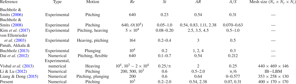
Table 1 lists relevant previous work on the rigid 3-D pitching of a rectangular panel with particular attention to the operating regime. Also, a few plunging, heaving and flexible cases are combined. It is apparent that most of these studies are primarily experimental, and that thus far numerical efforts have received relatively less attention. The pitching motions of 3-D rectangular foils reported in previous numerical simulations (Li & Lu Reference Li and Lu2012; Liang & Dong Reference Liang and Dong2015) are restricted to  $Re\leqslant 1000$, albeit with a fixed
 $St=0.6$. In contrast, the current work is a new contribution and relevant study on unsteady bio-inspired propulsion, providing a much larger range of
 $St$
 $(0.2\leqslant St\leqslant 2.0)$ than prior simulations, at reasonably high
 $Re$. The detailed 3-D flow structures near the panel, and pressure data obtained from our computations, leverage the strengths of the simulations to produce results that may be more challenging for experiments. It is appropriate to mention that Cleaver, Wang & Gursul (Reference Cleaver, Wang and Gursul2012) and Calderon et al. (Reference Calderon, Cleaver, Gursul and Wang2014) performed experiments on low-amplitude plunging NACA0012 aerofoil at high
 $St$, which resulted in wake flows very similar to those of pitching. They reported two lift-coefficient branches for high
 $St$ at a condition where the angle of attack is less than or equal to the stall angle. The upper and lower branches correspond to the upward and downward deflected jets (Cleaver et al. Reference Cleaver, Wang and Gursul2012). They observed a long series of vortex loops generated from a long ‘daisy chain’ of interconnected trailing edge vortices (Calderon et al. Reference Calderon, Cleaver, Gursul and Wang2014). The key research questions that have not been adequately addressed in the literature are as follows: (i) How does the enhancement in
 $St(>1)$ change the different shedding regimes observed near the trailing edge of the pitching panel? (ii) What are the underlying mechanisms of the secondary instabilities associated with the wake compression? (iii) How does the pressure field behave near the trailing edge of the panel? (iv) What are the space–time behaviour and frequency events associated with the pitching motion at this
 $St$ regime? (v) How do the force coefficients alter at these
 $St$ ranges? In the present research, we have explored these questions using 3-D computations at
 $Re=1000$ for
 $AR=0.54$ and 2.38.
List of previous studies for 3-D rigid pitching of rectangular panels. Here  $N_x,N_y,N_z$ are grids used in the numerical studies with lengths
 $L_x,L_y,L_z$. Note, few available 3-D numerical studies on pitching, heaving and plunging motions are mentioned together, whereas the present study primarily focused on the pitching motion only.

2. Physical system and numerical set-up
2.1. Physical system
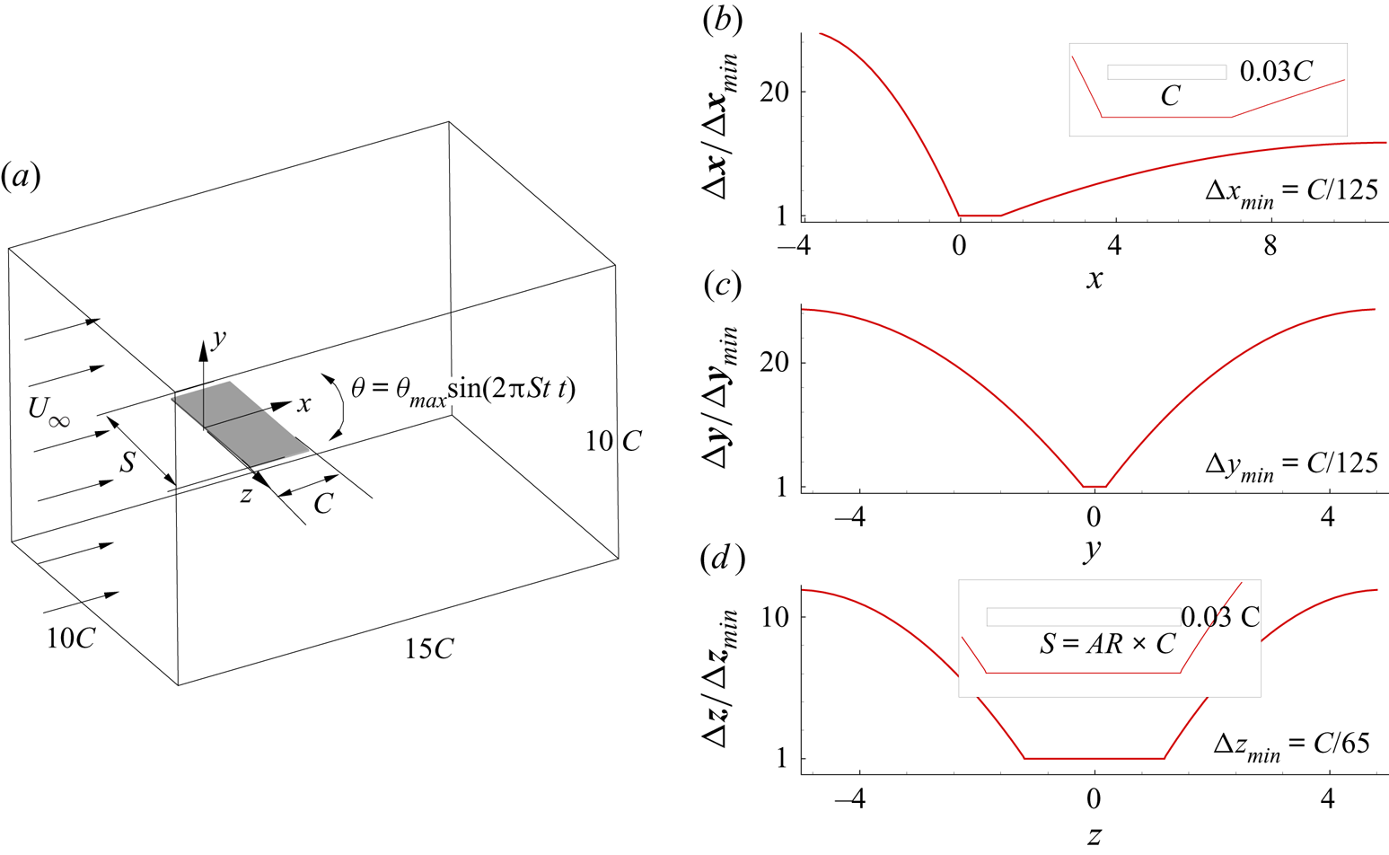
The physical problem involves the pitching of a thin rectangular rigid panel about its leading edge, placed in a uniform left-to-right flow ( $U_{\infty }$), as shown schematically in figure 1. The coordinate system is so chosen that the
 $x,y$ and
 $z$ axes point in the streamwise, cross-stream and spanwise directions, respectively. The pitching motion about the
 $z$-axis is described by the angular displacement
 $\theta (t)= \theta _{max} \sin ( 2{\rm \pi} ft)$ where
 $f$ is the pitching frequency and the maximum angular displacement is given by
 $\theta _{max }=\tan ^{-1}(A/{2C})$ where
 $A$ and
 $C$ are the double amplitude and chord of the panel, respectively. The control parameters for the problem are the aspect ratio given by the span-to-chord ratio
 $AR=S/C$, Reynolds number based on chord
 $Re=U_{\infty }C/\nu$ and the imposed non-dimensional pitching frequency
 $St=fA/U_{\infty }$. We selected the panel geometry and computational domain to best reproduce conditions in the low-aspect-ratio pitching panel experiments by Buchholz & Smits (Reference Buchholz and Smits2006, Reference Buchholz and Smits2008). Accordingly we limit
 $\theta _{max}=5^{\circ }$ and consider two aspect ratios
 $AR=0.54,2.38$ for a wide range of pitching frequencies
 $0.2 \leqslant St \leqslant 2$.
Schematic diagram showing a uniform flow past a rigid panel pitching about the leading edge with the extent of the domain. The variation of spatial grid resolution normalised by minimum mesh sizes  $( \Delta x,\Delta y,\Delta z )_{min}$ along
 $x$,
 $y$ and
 $z$ directions are shown at the right-hand-side panel. In the inset, panel geometry is shown in all the three planes.

2.2. Mathematical description
The governing equations for the problem are the constant property, incompressible mass and momentum conservation laws. The thickness of the panel is taken as  $3\,\%$ of the chord, which is placed in a domain that extends
 $15$,
 $10$ and
 $10C$ in the streamwise, cross-stream and spanwise directions, respectively. At the inlet, velocity is specified as
 $\boldsymbol {u}=(U_{\infty },0,0)$ coupled with a zero pressure gradient
 $\partial p/\partial x=0$. In order to keep the upstream feedback at a minimum level, a convective condition, given by
 $\partial (u,v,w)/\partial x=0$ is prescribed at the exit plane with a gauge pressure
 $p=0$. Boundary conditions at the shear-free vertical side boundaries read
 $\partial (u,v,p)/\partial z=0,w=0$, while the same marginally modifies to
 $\partial (u,w,p)/\partial y=0,v=0$ on the horizontal boundaries. Following the earlier pitching panel experiments (Buchholz & Smits Reference Buchholz and Smits2008; Kim et al. Reference Kim, Strom, Mandre and Breuer2017) and numerical studies (Liang & Dong Reference Liang and Dong2015) together with the experimental measurements on biological locomotion (Taylor, Nudds & Thomas Reference Taylor, Nudds and Thomas2003), we fixed the Reynolds number at 1000. All the cases are started from a no-flow state and allowed to settle to a dynamic steady phase. Once attained, nearly thirty shedding cycles are used to compute the time-averaged field which is used for all the analysis shown in later sections including circulations, pressure gradient and force coefficients. The thrust, lift and spanwise force coefficients are defined as (Buchholz & Smits Reference Buchholz and Smits2008),
 $C_{T,L,Z}=F_{T,L,Z}/(\frac {1}{2}\rho U_{\infty }^{2}S\,C)$ where
 $F_T$,
 $F_L$ and
 $F_Z$ are, respectively, the thrust, lift and spanwise force components acting on the panel.
2.3. Numerical set-up
The conservation equations, mentioned in the previous section, are solved using a non-staggered finite-volume technique where special treatment is incorporated to strengthen the velocity–pressure coupling. The second-order Adams–Bashforth scheme is used for the nonlinear convective terms, while the diffusive terms are handled implicitly using the Crank–Nicolson scheme in order infuse numerical stability into the overall time-integration strategy. All the spatial terms are approximated by second-order volume- or surface-integral approximations. The complex boundaries are resolved using the diffuse-interface immersed-boundary method (Pan & Shen Reference Pan and Shen2009; De Reference De2016, Reference De2018) where a volume-averaged unified discrete equation is solved everywhere in the domain, relaxing the conventional variable reconstruction near non-conformal boundaries for sharp-interface immersed-boundary techniques. The panel, surface triangulated with approximately 32 000 and 78 000 triangular elements for  $AR=0.54$,
 $2.38$, respectively, were found to predict the panel volume to nearly
 $1\,\%$ accuracy. A non-uniform Cartesian mesh with uniform grids in a volume that envelops the panel at all times was used for all the computations. The distribution of the grid spacing in all three directions is shown in the right-hand column of figure 1. The resulting sparse linear systems are solved to machine accuracy (
 $10^{-8}$) using the BiCGSTAB method, preconditioned by a highly scalable diagonalised version of Stone's strongly implicit procedure (SIP). The aforementioned numerical development has been achieved through a series of high-resolution complex geometry (De & Sarkar Reference De and Sarkar2020a,Reference De and Sarkarb; Kushwaha & De Reference Kushwaha and De2020) simulations. All cases are simulated using a time step of
 $\Delta t=5 \times 10^{-4}$, resulting in a maximum Courant number
 $Cu_{max}=0.15$ for
 $St=2$, which is found as a better trade-off between the speed and stability of the time-marching procedure. Total computational time for all the runs was nearly 0.16 million core hours on a 250 Teraflop SMP cluster.
In order to evaluate the effect of mesh refinement, the case with  $AR=0.54$ and
 $St=0.6$ was tested on four progressively refined meshes starting with
 $M_1=200 \times 85 \times 85$ and increased
 $25\,\%$ in each directions while keeping a small
 $\Delta t$ (
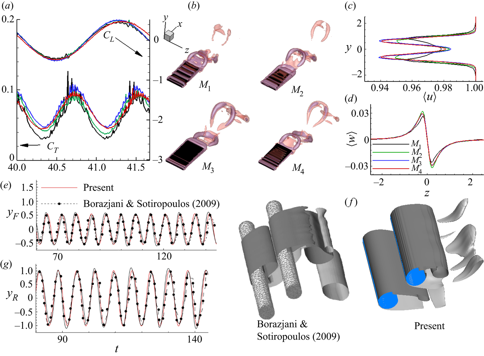
 $=10^{-4})$. The time evolution of the thrust and lift coefficients, instantaneous vortical structure and time-averaged streamwise and spanwise velocities are shown for all the meshes in figure 2(a–d). Notwithstanding that an increase in mesh size small scale oscillations appear in the thrust coefficient, both the time-averaged velocities and force coefficients exhibit mesh convergence at the upper limit of the chosen grids. The horseshoe vortical structure becomes increasingly clear with refinements in mesh, and at the upper limit they become nearly identical at
 $M_3$ and
 $M_4$. In view of better resolution of the wake, the finest mesh given by
 $400 \times 170 \times 170$
 $(AR=0.54)$ and
 $400 \times 170 \times 230$
 $(AR=2.38)$ was chosen for all subsequent calculations. In addition, to check the validity of the present numerical model, we solved a multi-object fluid-structure interaction (FSI) problem for a pair of identical 3-D vibrating circular cylinders, and compared results with the numerical results of Borazjani & Sotiropoulos (Reference Borazjani and Sotiropoulos2009). We carried out 3-D computations for a reduced velocity
 $U^{\ast }=4$, mass ratio
 $m^{\ast }=2$, and
 $Re=200$. The time evolution of the centroids of the upstream
 $(y_F)$ and downstream
 $(y_R)$ cylinders are compared in frame (e), while frame (f) shows the instantaneous spanwise vorticity
 $(\omega _{z}=\pm 1)$ iso-surfaces. Agreement is found to be in the range excellent to reasonable, given the complexity and difference in the solution technique of the reference.
Mesh convergence test results for four successively refined mesh sizes  $M_1$,
 $M_2$,
 $M_3$ and
 $M_4$ at
 $AR=0.54$,
 $St=0.6$. (a) Temporal evolution of the coefficients of lift
 $C_L$ and drag
 $C_D$. (b) Perspective views of the 3-D instantaneous vortical structures visualised by the
 $Q$-criterion (
 $Q=1$). (c) Variations of time-averaged streamwise velocity
 $\langle u \rangle$ in the cross-stream
 $(y)$ direction. (d) Variations of time-averaged spanwise velocity
 $\langle w \rangle$ in the spanwise
 $(z)$ direction. Panels (a), (c) and (d) have the same legends. Comparison of the present numerical set-up with Borazjani & Sotiropoulos (Reference Borazjani and Sotiropoulos2009) for vortex-induced vibrations of a pair of rigid cylinders with (e) time evolution of the centroids of the upstream
 $(y_F)$ and downstream
 $(y_R)$ cylinders and (f) instantaneous spanwise vorticity
 $(\omega _{z}=\pm 1)$ iso-surfaces.

3. Results and discussion
We performed numerical simulations at  $Re=1000$ to assess the implications of varying
 $St$ on the 3-D flow features of flow past a rigid pitching panel. We show the results by considering two illustrative values of aspect ratio in order to probe into the practical relevance of experimental conditions (Buchholz & Smits Reference Buchholz and Smits2006, Reference Buchholz and Smits2008) and biological locomotion (Richard Reference Richard1958; Ellington Reference Ellington1984; Taylor et al. Reference Taylor, Nudds and Thomas2003). First, we demonstrate the alternations in the wake–vortex development under the combined influences of
 $St$ and aspect ratio. Subsequently, we analysed the resulting circulation, secondary instability and discussed various other transition mechanisms.
3.1. Overview of wake vortex topology
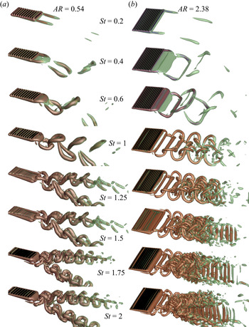
In figure 3, we plot the instantaneous vortical structures with  $St$ for
 $AR=0.54$ and 2.38. We visualised the wake vortices using iso-surfaces of
 $Q({=}1)$ (Jeong & Hussain Reference Jeong and Hussain1995). The vortex core region, which is depicted in red, has a smaller
 $Q$, which envelops the former. At
 $St=0.2$, we observe a stable attached flow situation. A flat shear layer extends from the trailing-edge corners owing to its low-speed motion and is subjected to pure diffusion-dominated growth. However, at
 $AR=2.38$, the streamwise length of the shear layers are found to be less than for
 $AR=0.54$. With increasing
 $St$, we observe a wake transition. The wake patterns at
 $St=0.4$ shows a slit-horseshoe vortex at
 $AR=0.54$, and a bow-shaped structure at
 $AR=2.38$. The vortex street remains attached to the panel owing to the induced velocity descending from the tip vortices at the trailing edge corners. At
 $St=0.6$, the wake topologies for
 $AR=0.54$ and 2.38 yield the formations of horseshoe and isolated bow-shaped vortices. Interestingly, at
 $St=1$, the wake carries conformity with a reverse von Kármán vortex street for both aspect-ratio panels. The formation of an interlocked chain of horseshoe vortices is seen at
 $AR=0.54$, whereas we find a bow-shaped vortex connected with secondary bridgelet-type structures (
 $z$-direction oriented structures that almost look like a corrugated surface on the panel) for
 $AR=2.38$. Although such structures are drawn in a sketch in Buchholz & Smits (Reference Buchholz and Smits2006, Reference Buchholz and Smits2008), experiments typically cannot resolve these near a body.
Influence of  $St$ on the wake vortex topology past a rigid pitching panel for
 $AR=0.54$ and
 $AR=2.38$. All 3-D perspective views of the vortical structures are visualised by plotting
 $Q$-criterion with
 $Q=1$. Note, all the instantaneous
 $Q$-criterion structures are shown at the same dimensionless instant.

At  $St=1.25$, the streamwise vortex from the trailing edge for
 $AR=0.54$ collapses within a shorter distance and splits, forming a bifurcating wake resembling a twin jet-type oblique flow pattern in the transverse direction. The horseshoe vortex shed from the trailing edge develops a perturbation before being bifurcated into a pair of jets. That, in turn, evolves to form a localised hairpin-like vortex signature, where the tip of the vortices is strong enough to keep the leading-edge vortex connected. In the spanwise direction, hairpins are convected in the transverse direction owing to self-induction. In contrast, at
 $AR=2.38$, we observe an increased strength of the bridgelets forming more dipoles than at
 $St=1$. The vortex filaments start interacting with each other via the thread-like connecting structures that connect two vortex filaments by wrapping around them. These structures eventually split farther downstream owing to spanwise instabilities (Visbal Reference Visbal2009) to form isolated pockets of vortex rings that rejoin with the small-scale bridgelets. We observe an analogous resemblance of wake structures between
 $St=1.5$ and 1.25 at
 $AR=0.54$. Higher stretching of the hairpin-vortex trains in the transverse direction is seen at
 $St=1.5$. The heads of the hairpin vortices are loosely connected with the already shed preceding hairpin tails. The wake structure at
 $AR=2.38$ exhibits rapid interactions of the threads, causing the bridgelets to grow into asymmetric vortex loops. The bridgelets undergo reconnection and, owing to self-induced motion, advect downstream. In this process, the regions of larger
 $|\boldsymbol {\omega }|$ in the primary vortex filament undergo rapid rotation and bring about a gross twisting of the vortex lines encompassing the bridgelets (Virk, Hussain & Kerr Reference Virk, Hussain and Kerr1995). A further effect of strong spanwise instabilities split these bridgelets along with the primary vortex loops, ultimately culminating in the development of isolated packets of parallel strips advecting in the streamwise direction.
We observe that the overall vortex dynamics become even richer and more complex beyond  $St>1.5$. For
 $St=1.75$, we see that the hairpin vortices at
 $AR=0.54$ transmute to ring-like vortex structures, yielding two distinct chains of alternating vortices each engulfed by the next downstream of it (Dai et al. Reference Dai, Luo, Ferreira de Sousa and Doyle2012; Li & Lu Reference Li and Lu2012). The vortex rings are oriented primarily in the streamwise direction and interlocked by hairpin-type vortex legs. As expected, the spanwise instabilities contribute to the initial circular core of the rings and deform into braid-like structures. A further increase in
 $St$ causes the rotation of the vortex rings, which are inclined in the transverse direction at
 $St=2$. The rings travel downstream under self-induction, which again deform and recede via spanwise instability-driven cross-diffusion. For
 $AR=2.38$, the bridgelets undergo successive reconnection and stretching with the primary shed vortices triggered by the strong spanwise instability at
 $St=1.75$. These reconnections encourage the evolution of swirling rings of vortices and then again deform into complex structures, cause the generation of smaller vortex filaments, and thereby promote the wake into an avalanche of 3-D vortex structures. Interestingly,
 $St=2$ yields a much complicated wake topology, showing a transverse asymmetrically bifurcated wake rolling over the parallel strips. The isolated arrays of parallel strips are now produced at a much earlier stage and are broadly dominated by the remaining vortex filaments that survived during the wake cloud formation. Irrespective of aspect ratio, the streamwise spacing of the vortex structures is reduced with increasing
 $St$ (Dai et al. Reference Dai, Luo, Ferreira de Sousa and Doyle2012; Li & Lu Reference Li and Lu2012).
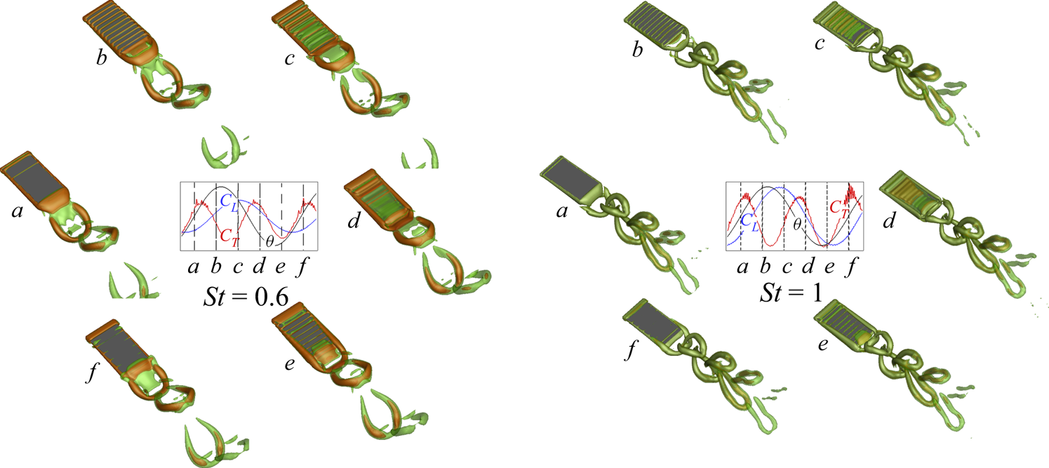
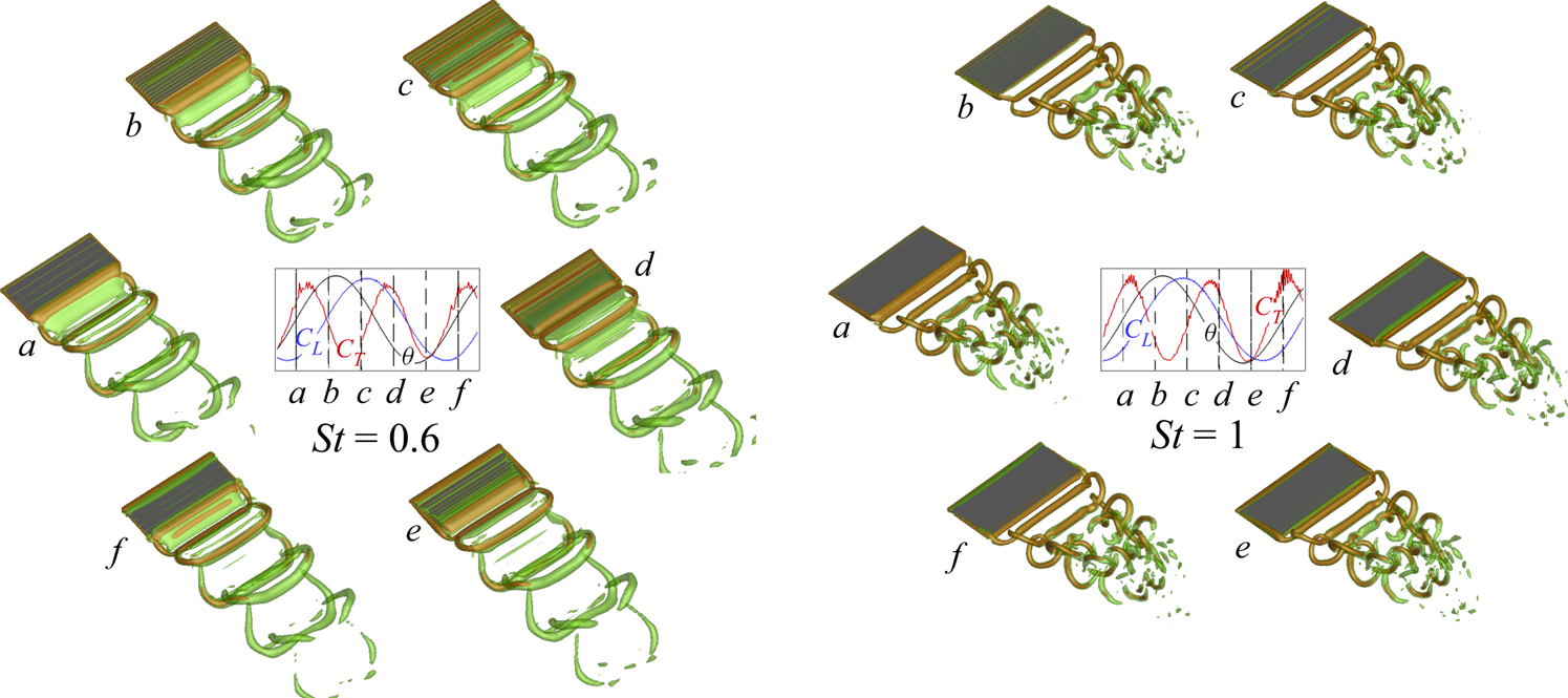
In figures 4 and 5 we describe periodic evolution of the vortex street based on the  $Q$-criterion for
 $St=0.6, 1$, at
 $AR=0.54$ and 2.38, respectively. In a complete pitching cycle, the temporal evolution of vortices corresponding to the instances (a–f) are indicated in the insets on
 $\theta$,
 ${C_T}$ and
 ${C_L}$ time series. At
 $St=0.6$, the pitching cycle starts with formations of the horseshoe
 $(AR=0.54)$ and bow-shaped
 $(AR=2.38)$ vortices without connecting their tips by peeling off the spanwise shear layers accumulating at the trailing edge. The tip of the vortices at this lower
 $St$ lack strength and, as a result, the mutual induction process responsible for linking the tips deteriorates. It may be pointed out that the vortex connections visualised depend on the values of
 $Q$ plotted for the iso-surfaces. A smaller
 $Q$ value would probably show increased connections (in agreement with the point that they are weaker here). During the upward stroke
 $(\theta \to \theta _{max})$, the shear layers accumulate to form a convex shape and cause an extension of the panel surface farther into the wake, allowing an auxiliary growth of the vortices before detachment. The instant the vortex strand grows into its developed stage, the strand connecting the boundary layer with the local vorticity extreme experiences a strong strain rate dominated constriction mechanism. In effect, the strand commences a detachment process from its source near to
 $\theta \approx \theta _{max }$. This is followed by pinching off a coherent horseshoe (or bow-shaped at
 $AR=2.38$) vortex in the upward direction of the panel owing to upward-induced velocity near to
 $\theta \approx \theta _{c}$, which gradually moves in the streamwise direction with the downstream advection of the flow. It is worth mentioning that the area over which this constriction process occurs is governed by the positive strain-rate parameter
 $\gamma >0$ where
 $\gamma \approx \textrm {tr}(D^2)$ and the rate-of-strain tensor
 $D=(\boldsymbol {\nabla } \boldsymbol {u} + (\boldsymbol {\nabla } \boldsymbol {u})^\textrm {T})/2$ (Biswas & Sarkar Reference Biswas and Sarkar2009).
Perspective views of the 3-D periodic vortex shedding cycle showing  $Q=1$ surfaces at
 $AR=0.54$ for
 $St=0.6$ and 1. The temporal evolution of vortices from the trailing edge of the panel is shown in the instances (a–f) indicated on the time series of
 ${C_T}$,
 ${C_L}$ and
 $\theta$ in the insets.

Perspective views of the 3-D periodic vortex shedding cycle with  $Q=1$ surfaces at
 $AR=2.38$ for
 $St=0.6$ and 1. In the insets, the temporal evolution of vortices from the trailing edge is shown in the instances (a–f) indicated on the time series of
 ${C_T}$,
 ${C_L}$ and
 $\theta$.

The vortex formation during the downward stroke  $(\theta \to \theta _{min})$ follows an analogous route, except that the downstream induced velocity causes the shed vortical structure to roll towards the downward direction of the panel at approximately
 $\theta \approx \theta _{f}$. At
 $AR=2.38$, the disconnected tip of the bow-shaped vortices start to interact with the legs of the already shed vortices post detachment. This interaction causes a gradual reduction of the downward velocity induced by the shed vortices thereby forming bridgelet-type structures at higher
 $St$, whereas at
 $AR=0.54$, isolated horseshoe vortex structures become apparent. Note that we witness the formation of two vortices per pitching cycle for both
 $St$ (Buchholz & Smits Reference Buchholz and Smits2006, Reference Buchholz and Smits2008). At
 $St=1$, the pitching cycle results in the formation of a chain of horseshoe and bow-shaped vortices interlocked together to emerge as a reverse von Kármán vortex street for
 $AR=0.54$ and 2.38. The overall formation dynamics are analogous to the one at
 $AR=0.54$, although the period is smaller in terms of the occurrence of wake vortex structures for
 $St=1$. The bow-shaped structure shed outward from the trailing edge is connected with the hitherto shed vortices with secondary bridgelet-type structures. This occurs owing to the mutual induction of instantaneously generated threads, which advect faster than the primary vortex loops. As the vortices convect farther downstream, the bridgelets split owing to the development of the spanwise instabilities, and, in consequence, leave behind discrete packets of vortex contrails. Farther downstream the wake appears weaker and dissipated for
 $St=1$. Nevertheless, the vortex configuration governs the extent of the wake coherence and is regulated by the shear layers released from the trailing edge. We also observe from the insets that regardless of aspect ratio and
 $St$, that
 $\theta _c$, corresponding to the separation of the trailing-edge vortices during upward stroke, is always nearer to the maximum lift
 $({\sim}C_{L_{max }} )$ and minimum thrust
 $({\sim}C_{T_{min }} )$ point. In contrast, we find an inverse relationship during the downward stroke of the pitching cycle.
3.2. Circulation of the wake
We calculated the dimensionless circulation along the spanwise  $\varGamma _z=\int _{\varOmega _z}{(\boldsymbol {\nabla } \times \boldsymbol {u})\boldsymbol {\cdot } \hat {n}_z\,\textrm {d}\varOmega _z}$ and streamwise
 $\varGamma _x=\int _{\varOmega _x}{(\boldsymbol {\nabla } \times \boldsymbol {u})\boldsymbol {\cdot } \hat {n}_x\,\textrm {d}\varOmega _x}$, directions using the time-averaged velocity (see § 2.2), where
 $\hat {n}_x$ and
 $\hat {n}_z$ denote unit normal vectors along
 $x$ and
 $z$ directions. We computed circulation values for the domain-independent regions
 $\varOmega _x \equiv ( y\times z )\equiv \{ ( 0, 4 )\times ( 0, 3.5 ) \}$ and
 $\varOmega _z \equiv ( x\times y )\equiv \{ ( 1.1, 8 )\times ( 0, 4 ) \}$. It should be noted that
 $\varGamma _x$ and
 $\varGamma _z$ only account for half the span and transverse plane (because the circulation over the entire span or plane would be zero).
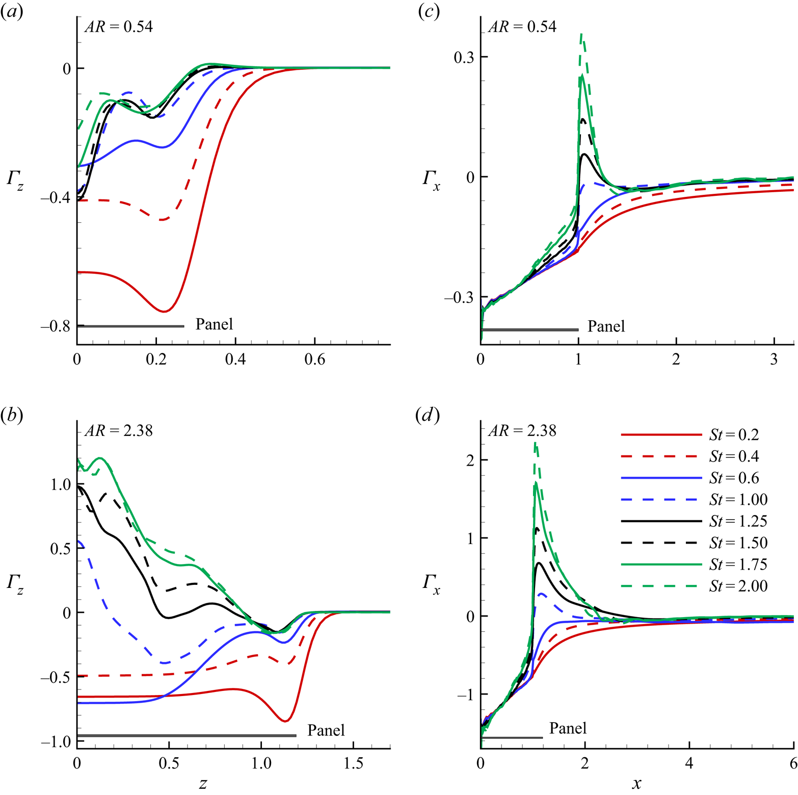
In figure 6, we show the dependence of  $\varGamma _z$ and
 $\varGamma _x$ on
 $St$ for different aspect ratios. In general, the circulation strength increases with increasing
 $St$, and is a strong function of
 $AR$. We observe from figure 6(a) that at
 $St=0.2$,
 $\varGamma _z$ decreases monotonically from the centre of the panel to its local minimum nearer to the edge. After that, it increases progressively to zero at approximately
 $z\approx 0.6$, a region beyond the zone of influence of the shed vortices. For the negative directional growth in
 $\varGamma _z$, see figure 3, the attached shear layers formed at the trailing edge are seen to play their role. At
 $St=0.2$, only a few circulation loops, distributing a larger spanwise area evolve at the trailing edge with a strong localised counter-clockwise rotation. This leads to an enhancement of the circulation strength and makes the region prone to negative growth. Beyond the minimum point, the overall circulation strength reduces owing to the reduction in spanwise diffusion of the shear layer. Therefore, the local circulation shows an asymptotic increase in the positive direction until a zero value is reached near the zone of influence. We observe that
 $\varGamma _z$ curves essentially collapse across
 $z$ for
 $St>0.6$. At
 $St\geqslant 1$, the formation of multiple tangled vortices are more enhanced, and, through mutual inductions, eventually results in a reduction in circulation strength.
Dimensionless wake circulation along the spanwise  $(\varGamma _z)$ and streamwise
 $(\varGamma _x)$ directions for various
 $St$. Results are shown at aspect ratios of (a,c) 0.54 and (b,d) 2.38, respectively. The proportionate panel dimensions corroborating each aspect ratio are also indicated.

In contrast to  $AR=0.54$, we observe an entirely different trend of
 $\varGamma _z$ at
 $AR=2.38$. Figure 6(b) shows that the characteristic behaviour of
 $\varGamma _z$ for
 $St=0.2, 0.4$ is negative at
 $AR=2.38$ and does not change with the aspect ratio. The value of
 $\varGamma _z$ is nearly flat and only shows higher values (negative direction) closer to the edge of the panel. At
 $St>0.6$, near the central region of the panel,
 $\varGamma _z$ exhibits positive maxima, but shows negative minima for
 $AR=0.54$. In addition, the spanwise variations in
 $\varGamma _z$ at
 $AR=0.54$ become increasingly higher, although, at
 $AR=2.38$, it drops along
 $z$. Hence, the character of the wake for these aspect ratios is different from that expected from the measured circulation. Interestingly, the boundary point of the wake zone of influence
 $(\varGamma _z=0)$ moves towards the central region of the panel with increasing
 $St$, indicating that wake compression is prevalent owing to the competitive effects between aspect ratio and
 $St$. Accordingly, we observe a much smaller zone of influence at
 $AR=2.38$ than
 $AR=0.54$ for larger
 $St$. For
 $St>0.6$, an increased secondary instability causes fluid particles at the edge to break up and approach the central wake region. This triggers a wake compression by increasing the spanwise movement of the flow at higher
 $St$. The flow attempts to compress and converge towards the central region, and a negative pressure region along the wake width develops. As a result, the intensity of
 $w$, which is responsible for wake compression, increases, thereby causing the wake activity to be constrained within a narrow band in the spanwise direction. The wake tends to form a concentrated core region constituting intense localised vorticity distribution. This may be conditional on large
 $St$ situations where the vorticity has higher strength. In the compressed wake, the velocity at the central region is less than that of the side wake region. The side wake remains unperturbed, but the core region constituting the compressed wake moves very slowly. This results in less diffusion of the compressed vortices, because for diffusion to occur vortices have to encounter a high-velocity region. Again, as the vortices are compressed, the chances of cancellation of positive and negative vortices becomes lower, yielding a fewer number of high-intensity circulation cells within a smaller area. Therefore, the core region possesses the maximum circulation magnitude, which is shown in figure 6(b).
We observe from figure 6(c,d) that  $\varGamma _x$ increases from the leading edge of the panel to its saturated value of
 $\varGamma _x=0$ far downstream. The circulation curves for
 $0.2\leqslant St \leqslant 0.6$ exhibit smooth variations, whereas, for
 $St>0.6$, we notice a discontinuity in the
 $\varGamma _x-x$ distribution, which yields a sudden jump near the trailing edge. We see that the streamwise variation of
 $\varGamma _x$ from the leading edge grows almost linearly without showing any discernible differences with changing
 $St$. This phenomenon is attributed to the development of a sheet-like unsteady shear layer at the hinged plane, shed from the leading edge, which is found to be
 $St$-invariant. Near the trailing edge, a bifurcation in the
 $\varGamma _x$ distribution is attributable to higher values of angular velocity of the isolated vortex structures just after detachment. This eventually leads to an enhancement of linear velocities at higher
 $St$. The overall influence culminates in a discontinuity in the
 $\varGamma _x$ profile. Beyond the region of discontinuity, the formation of small-scale vortex structures, of lower circulation strength, are the sole contributors of a progressive decay of
 $\varGamma _x$. As a result, there is a gradual reduction of
 $\varGamma _x$ up until a threshold streamwise location is reached, beyond which
 $\varGamma _x$ shows axial invariance. At this point further cascading of circulation loops, owing to secondary instabilities, nullify each other, which results in
 $\varGamma _x=0$.
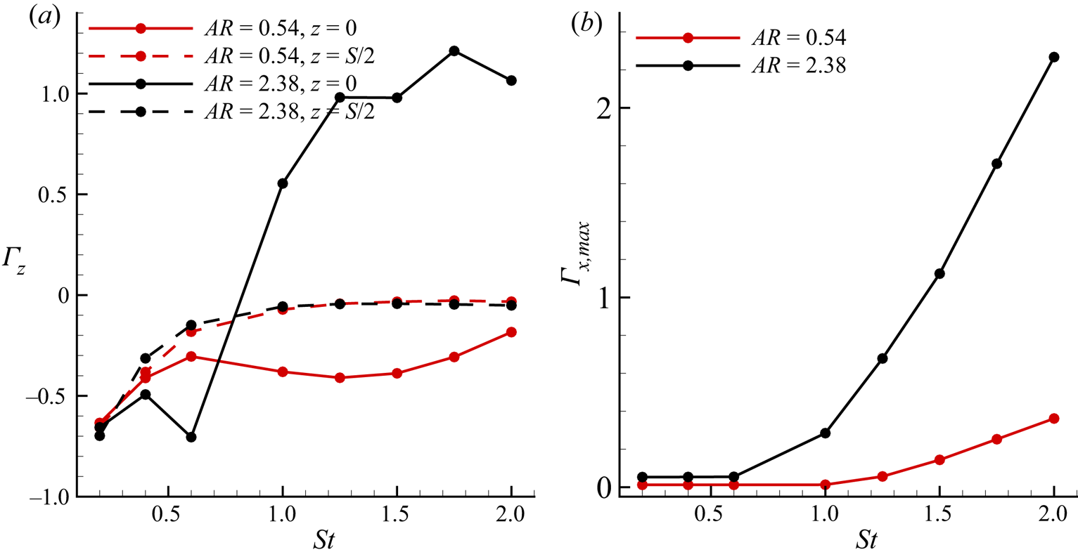
In figure 7(a) we show the dependence of  $\varGamma _z$ as a function of
 $St$ at the central plane
 $(z=0)$ and edge
 $(z=S/2)$ of the panel for
 $AR=0.54$, 2.38. We found that an increase in
 $St$ increases the circulation strength. Beyond
 $St>0.6$, there is a wake compression with fewer heavily squeezed high-intensity circulation cells at the central plane of the
 $AR=2.38$ panel. This behaviour is observed in 7(a), which shows that for all cases,
 $\varGamma _z$ increases progressively with
 $St$. In contrast, beyond
 $St>0.6$ of the high-aspect-ratio panel, a peak enhancement in
 $\varGamma _z$ at
 $z=0$ is observed. Interestingly, at
 $z=S/2$, the magnitude of
 $\varGamma _z$ for both aspect ratio panels approaches zero at large
 $St$. This is because of the increased tangled vortices triggered by the gradual enhancements of the spanwise instabilities at higher
 $St$ values. To show the influence of
 $St$ on the maximum streamwise vorticity transport leading to changes in circulation, we plot variations of
 $\varGamma _{x,max}$ with
 $St$ in figure 7(b) for both aspect ratios. We observe that with an increase in
 $St$, there is a monotonic increase of
 $\varGamma _{x,max}$, whereas the peak enhancement is always at
 $AR=2.38$. This explains the rapid augmentation in
 $\varGamma _x$ with
 $St$ shown in figure 6(c,d). However, for
 $St\leqslant 0.6$,
 $\varGamma _{x,max}=0$, comparable with the maximum
 $\varGamma _x$, which is mostly dominated by the negative values within that regime. Notably, the span of negative
 $\varGamma _x$ for
 $AR=0.54$ is expanded till
 $St\leqslant 1$, giving
 $\varGamma _{x,max}=0$.
(a) The influence of  $St$ on the dimensionless spanwise circulation for various spanwise locations corresponding to different aspect ratios. (b) The effect of
 $St$ on the maximum dimensionless streamwise circulation
 $(\varGamma _{x,max})$ for different aspect ratios.

3.3. Secondary motion
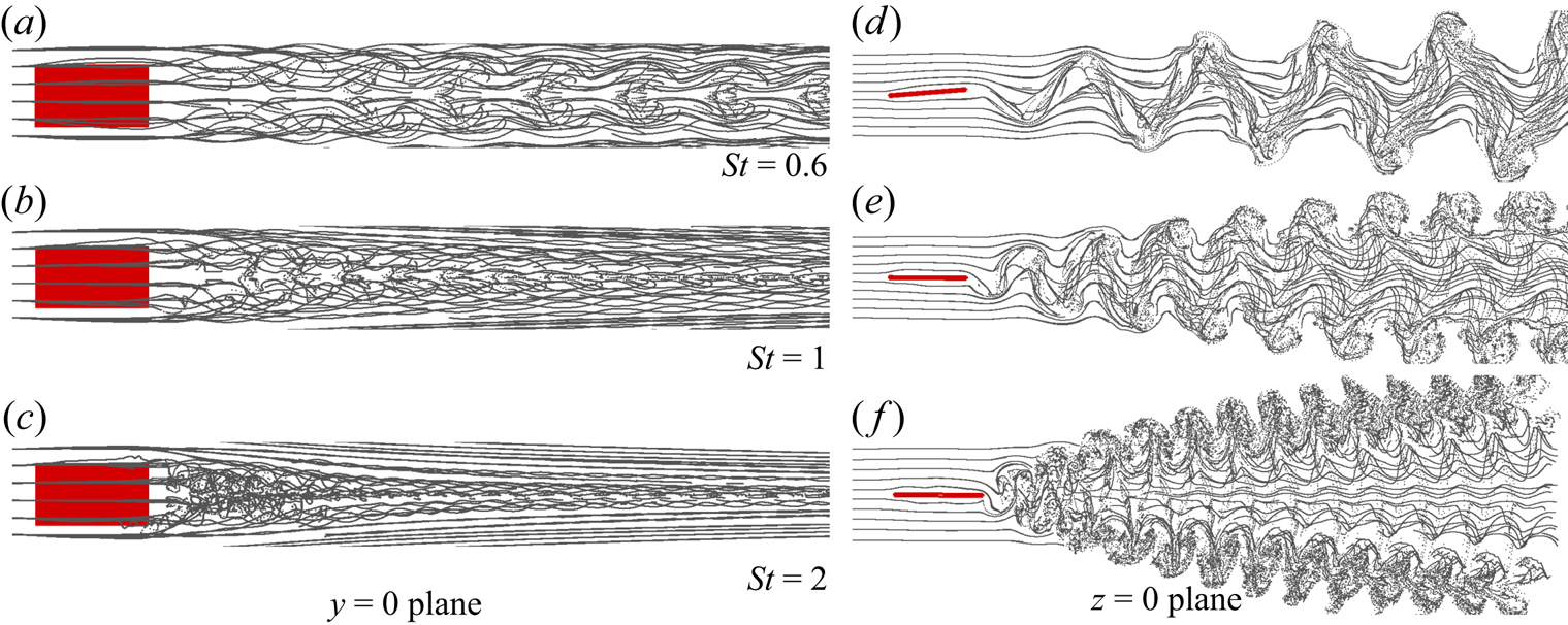
Secondary motion is the manifestation of the secondary instability, which arises primarily owing to end effects during the pitching motion. For different  $St$, figures 8–9 present streakline visualisations at
 $y=0$ (panel (a–c)) and
 $z=0$ (panel (d–f)) planes. For both aspect ratios, we observe a clear indication of the secondary motion from the streaklines. It shows that streaklines from the wide end of the panel start interacting with those of the narrow end slightly downstream of the trailing edge. Notably, the upstream flow displays a weak secondary motion. However, farther downstream of the trailing edge, a rapid spanwise movement of the streaklines, brought about by the higher degree of vortex interactions, causes spanwise compression of the wake width. With an increase in
 $St$, the inception of the secondary motion tends to move towards the trailing edge of the panel. It, therefore, triggers its strength, which also makes the wake expand along the panel's normal direction (Buchholz & Smits Reference Buchholz and Smits2008).
Streakline visualisations of the flow for  $AR=0.54$ and at different
 $St$. The plan view of the motion is shown in (a–c) (
 $y=0$ plane), whereas (d–f) show an end view of the motion (
 $z=0$ plane). The strong secondary motions are noticed from the plan view, which shows progressive wake compression with increase in
 $St$.

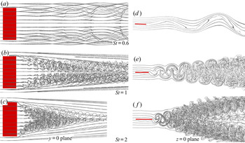
Streakline visualisations for  $AR=2.38$ and at different
 $St$. The plan view of the motion (
 $y=0$ plane) is shown in (a–c), whereas (d–f) show an end view (
 $z=0$ plane) of the motion.

It is to be noted that the combination of pitching motion and end effects promote the onset of 3-D instabilities. We infer from figures 8–9 that for  $AR=0.54$, because the spanwise length is small, such 3-D instabilities can interact with each other, making the central region less stable. In contrast, the end effects from the two sides hardly reach the central region at
 $AR=2.38$. Closer to the central region, flow is nearly two-dimensional (2-D), and only tends to become 3-D when the end effects encroach. Thus, for
 $AR=2.38$, we clearly see that near the central region, the flow remains 2-D for smaller
 $St$. However, because wake compression occurs at higher
 $St$, the instabilities growing from the two edges spin towards the central region, making it a 3-D flow. Interestingly, a lower value of
 $St$ appears to promote large-wavelength streamwise undulations, which are even more prominent at
 $AR=2.38$, while small-scale instabilities are characteristic of an increasing
 $St$. Thus, the wavelength of the undulations become smaller for increasing
 $St$, which essentially signifies that high wavenumber disturbances are become more critical at higher
 $St$.
In the vertical planes of figures 8–9, the top and bottom shear layers diverge. Therefore, the wake width increases with increasing  $St$. The extremities of the shed shear layers form spokes which are symmetrically placed about the central region of the panel. These spokes are seen to become unstable earlier than the rest of the flow and are more explicit at higher
 $St$. For large the aspect ratio the flow behaves strangely at smaller
 $St$, where we notice the flow to exhibit clear signs of conventional bluff-body motion, and manifest as the entire wake vibrating with the same global frequency. However, as
 $St$ increases, a vertical bifurcation of the wake appears, which we have commonly termed as the oblique twin jet-type flow pattern. As we can see, higher values of
 $St$ result in denser jets. An increase in
 $St$ leads to a stable central region, and hence, it causes a higher concentration of small-scale wake structures at the jet plane through an effective transport from the central zone. The streaklines show a clear picture of the reverse von Kármán vortex street. We further found that the flow has an apparent similarity at higher
 $St$ for both aspect ratios, but at lower
 $St$, they show entirely different behaviour. It is important to note that the three-dimensionality of the wake structures is local in nature, and is seen more at higher
 $St$, where it is observed to be non-uniform across the entire wake width in both spanwise and cross-stream directions. The consequence of this is the localisation of non-uniform 3-D instabilities in both spanwise and cross-stream directions.
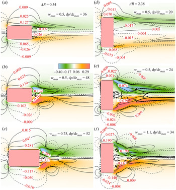
In figure 10, we show the time-averaged  $w$ contours, where
 $\textrm {d}p/\textrm {d}z$ is overlaid to obtain a possible relationship between them. It is apparent from the figure that the intensity of secondary motion increases with
 $St$. The spanwise velocity does not change significantly, even at moderate
 $St$ and is only seen to increase rapidly at very high values of
 $St$. In contrast,
 $\textrm {d}p/\textrm {d}z$ does not change significantly with
 $St$. As we can see, the maximum magnitude
 $(\textrm {d}p/\textrm {d}z)_{max}$ remains relatively constant. At
 $AR=2.38$, while the maximum spanwise velocity almost doubles at
 $St=2$, an only marginal increase in the
 $\textrm {d}p/\textrm {d}z$ is found to come about. Although we observe both favourable and adverse pressure gradients on either side of the central plane in the spanwise direction, the character of the secondary motion shows a symmetric distribution. This, perhaps, indicates that the growth of secondary motion cannot be directly connected to
 $\textrm {d}p/\textrm {d}z$; note that large
 $\textrm {d}p/\textrm {d}z$ and a high-intensity
 $w$ are seen to coexist locally in the near-wake region, and the two-dimensionality of the flow is again supported by very low-intensity
 $w$ magnitudes near the central region of the panel. The negatively correlated secondary motion on either side of the central zone re-emphasises strong wake compression at higher
 $St$. The pressure gradients are seen to be relatively smooth, even near the edge of the panels, which does not indicate a direct relationship between the secondary instability and the pressure gradient existing locally. Thus, the growth of the secondary instabilities has a greater connection to the intrinsic instabilities than the spanwise pressure gradients.
Isocontour lines of time-averaged spanwise pressure gradient  $(\textrm {d}p/\textrm {d}z)$ superimposed on the colour map of the time-averaged spanwise velocity for (a)
 $St=0.6$, (b)
 $St=1.5$, (c)
 $St=2.0$ for
 $AR=0.54$ and (d)
 $St=0.6$, (e)
 $St=1.5$, (f)
 $St=2.0$ for
 $AR=2.38$.

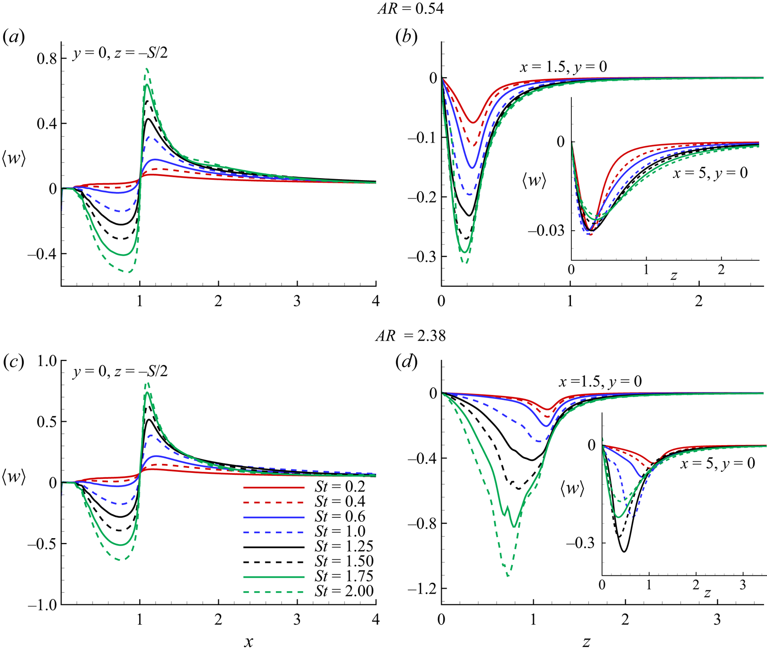
In figure 11, we plot the streamwise and spanwise distributions of time-averaged spanwise velocity  $\langle w\rangle$ as a function of
 $St$ for different aspect ratios. As evident from frames 11(a,c), the intensity of the secondary motion increases several times with increasing
 $St$, with a nearly discontinuous jump at the trailing edge of the panel. This trend is attributable to the high cross-stream velocity at the trailing edge, where the radius of motion is maximum. At
 $St=2$, such behaviour leads to a larger spanwise velocity, which is seen to be nearly discontinuous. However, at lower values of
 $St$, the intensity of the spanwise velocity is far lower. In a time-averaged sense, the nature of the spanwise velocity does not change appreciably at the higher aspect ratio; only the intensity of the flow increases marginally. However, in the spanwise direction, we observe from frames 11(b,d) that
 $\langle w\rangle$ increases dramatically. At higher
 $St$, as the wake compression occurs, the maximum spanwise velocity front moves towards the central region of the panel. This event is reflected in the
 $\langle w\rangle -z$ plot. We observe that the maximum spanwise velocity peak approaches closer to the spanwise direction for increasing
 $St$ and marginally reaches the central plane. A similar phenomenon is repeated at
 $AR=2.38$. However, in the near wake
 $(x=1.5)$, the magnitude of maximum spanwise velocity for
 $AR=2.38$ is nearly four times that of
 $AR=0.54$. In the far wake
 $(x=5)$, it even increases by approximately 10 times. Therefore, we conclude that the growth of secondary motion in the streamwise and spanwise directions does not obey an analogous route. In the streamwise direction, it follows the maximum magnitude. Whereas, in the spanwise direction, the magnitude is several times higher, from smaller to higher aspect ratios. We found that the organisation of the far wake is lost owing to the formations of tangled vortices. This is clear from frame (d), where it is seen that the highest velocity does not appear at the highest
 $St$. Whereas, at the lower aspect ratio (frame (b)), all the spanwise velocities nearly converge. Hence, the spanwise motion decays faster at the smaller-aspect-ratio panel. Interestingly, the secondary motion peaks near the edge of the
 $AR=0.54$ panel. In contrast, for
 $AR=2.38$, it decays significantly by the time it reaches the edge of the panel. Therefore, the decay in spanwise velocity only starts beyond the edge of the
 $AR=0.54$ panel. By comparison, decay starts within the width of the panel for
 $AR=2.38$. This also indicates the tendency of increased wake compression at higher aspect ratios.
Time-averaged spanwise velocity  $(\langle w\rangle )$ distribution in the streamwise direction
 $(x)$ for different
 $St$ and at a spanwise location of
 $y=0$,
 $z=-S/2$ (a,c). Time-averaged spanwise velocity
 $(\langle w\rangle )$ distribution in the spanwise direction
 $(z)$ for different
 $St$ and at a streamwise location of
 $x=1.5$,
 $y=0$; the inset shows values at
 $x=5$,
 $y=0$ (b,d). The top and bottom figures show results for
 $AR=0.54$ and
 $2.38$.

In frames 11(a,c), we observe that for  $x>1$, the flow moves in the positive
 $z$ direction. Because
 $\langle w\rangle _{x>1}>0$ at
 $z=-S/2$, this clearly signifies a positive
 $z$ directional motion of the fluid as a consequence of the spanwise wake compression. In contrast, the flow shows completely different behaviour near to the edge of the panel at
 $x<1$, where we notice
 $\langle w\rangle _{x<1}<0$. Thus, the fluid is diverging away from the panel. We analyse this behaviour in a situation when the momentum of the panel is imparted to the fluid during its pitching motion. As the momentum of the panel is very high, it pushes the fluid away. However, beyond the panel, the fluid approaches the central region because of wake compression. Thus, up to the trailing edge, it deflects the fluid outwards because of the high momentum of the panel. While beyond the trailing edge, because of wake compression, fluid rushes towards the central region. In other words, fluid first displaces and then again reverts to its original location. Such outboard motion induced above the panel is simply a consequence of conservation of mass. We note that the outboard motion of the fluid is nearly 50 %–60 % of the inward motion.
3.4. Frequency spectrum and space–time behaviour
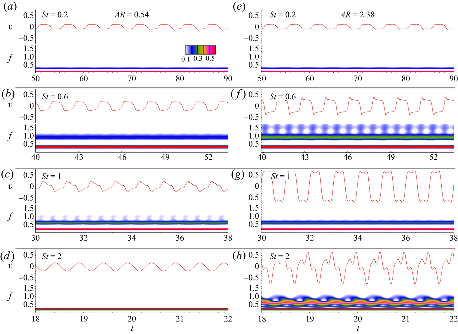
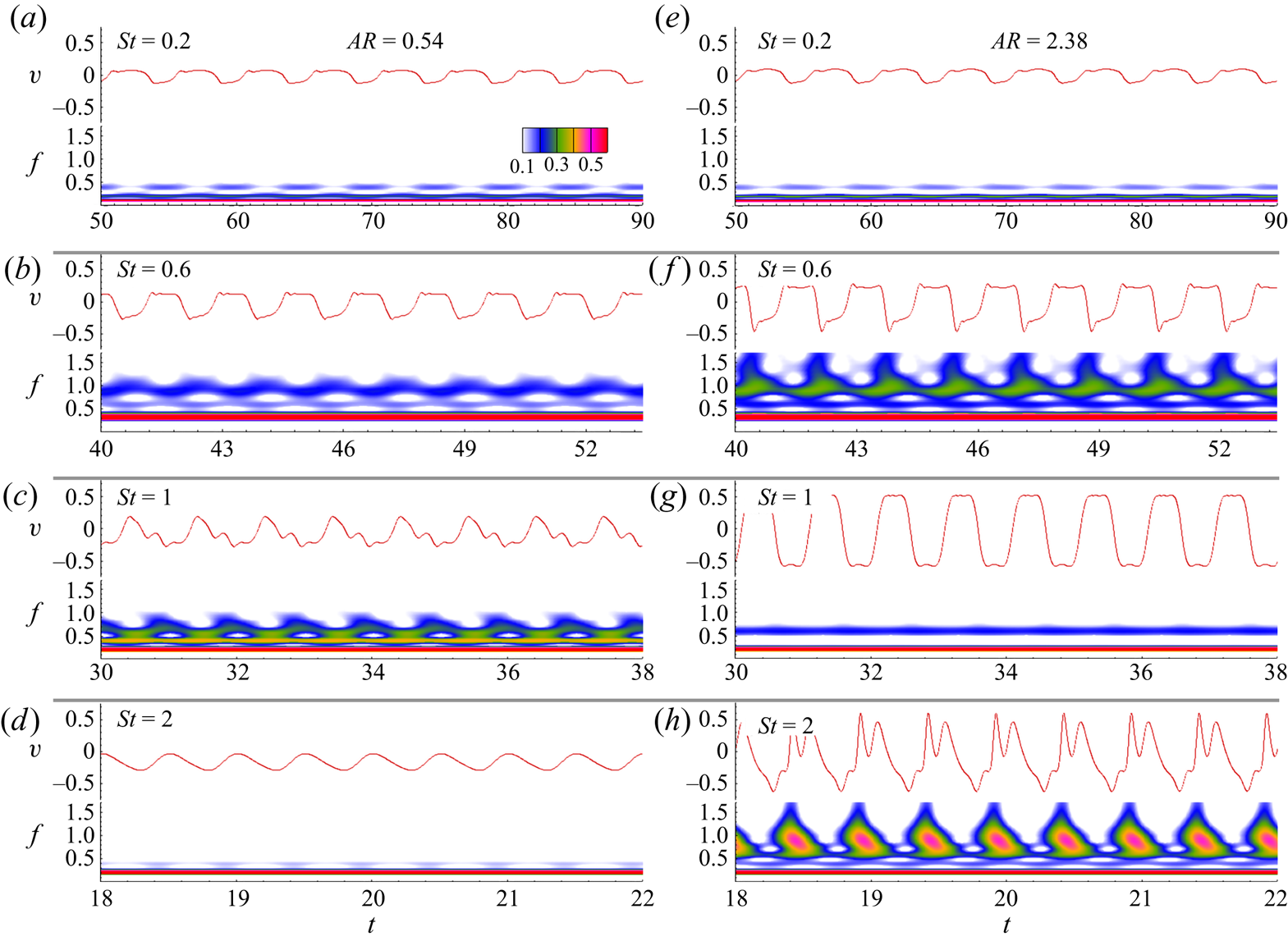
We analyse the spreading and timing of the frequency spectra by carrying out a continuous wavelet transform (CWT) of the cross-stream velocity signals at sampling locations,  $(2C,0,0)$ and
 $(2C,-y_{max},0)$. In CWT, the coefficient
 $c$ is generated with position (
 $\tau$) and scaling argument (
 $s$) as,
 $c(s,\tau )=(1/\sqrt {|s|})\int _{-\infty }^{\infty } f(t) \overline {\psi (t-\tau )/s} \,\textrm {d}t$. Where,
 $\bar {\psi }$ is the complex conjugate of the mother wavelet
 $\psi (t)=\textrm {e}^{-t^2/2}\cos 5t$ and
 $f(t)$ is the pseudo-frequency (De & Sarkar Reference De and Sarkar2020a,Reference De and Sarkarb).
The unsteady frequency distribution coloured by the normalised coefficient is shown in figures 12–13 for various  $St$ and aspect ratio. The source time-series data are also shown above the CWT map. Depending upon the magnitude of
 $St$, the shedding mode is observed to expand from a localised low-frequency to high-frequency mode. In figure 12, we notice that at
 $St=0.2$, the entire frequency spectra is dominated by the lower frequency modes and are synchronous with the pitching motion of the panel. Similar behaviour is noted for a higher aspect-ratio panel. However, a narrow band of slightly higher frequency modes is also apparent, but their strength is less than the primary modes. Thus, it has a negligible impact on the overall shedding characteristics. At
 $St=0.6$, the increased width of the high-frequency band takes larger values by shifting farther away from the primary lower-frequency band at
 $AR=0.54$. In contrast, at
 $AR=2.38$, apart from the high-frequency secondary spectrum, intermittent wavelet structures of a larger frequency tertiary spectrum are distributed over the entire period. At
 $St=1$, along with the thin band of low-frequency spectrum, lower aspect ratio also exhibits a secondary high-frequency spectrum distributed over a larger bandwidth. An analogous spectrum is apparent for
 $AR=2.38$ as well; although, the secondary spectrum has reduced bandwidth. We see that at
 $St=2$, a band of low-frequency spectrum thoroughly dominates over the entire period for
 $AR=0.54$. Therefore, indicating the complete periodicity of the vortex shedding synchronised with the
 $St$ of the motion. Whereas, for
 $AR=2.38$, along with the dominating low-frequency spectrum, a shallow band of low- to high-frequency wavelet structure is observed.
The CWT of the  $y-$velocity signals
 $(v)$ at a sampling location of
 $(2C,0,0)$. For the various
 $St$, CWT results are shown at
 $AR=0.54$ (a–d) and
 $AR=2.38$ (e–h) with each panel containing the source time series and CWT map. The colour map of the coefficients normalised by the global maximum is shown in the time-pseudo-frequency domain,
 $t-f$, depicting the influence of
 $St$ on the localised frequency concentration.

The CWT of the cross-stream velocity signals  $(v)$ at a sampling location of
 $(2C,-y_{max},0)$. For various
 $St$, CWT results are shown at
 $AR=0.54$ (a–d) and
 $AR=2.38$ (e–h) with each panel containing the source time series and CWT map. The colour map of the coefficients normalised by the global maximum is shown in the time-pseudo-frequency domain,
 $t-f$, depicting the influence of
 $St$ on the localised frequency concentration.

The CWT results in figure 13 shows  $St$ to be dependent on the multi-modal frequency signature. We observe a family of multiple high-frequency spectra at
 $St=0.2$ with the band splitting of the spectrum at larger frequency levels. Thus, indicating lateral diffusion of multiple low-frequency cells in the transverse direction. At
 $St=0.6$, along with the lower frequency cells, we see a family of multiple large-frequency spectra distributed over oscillating bandwidths at
 $AR=0.54$. The peaks of the oscillating bandwidths stretch farther at the higher frequency modes for
 $AR=2.38$, yielding wavelet structures related to the localised change in the shedding frequencies. At
 $St=1$, the spectral characteristics of the higher-aspect-ratio panel for both of the sampling locations show similar behaviour. In contrast, at
 $AR=0.54$, we notice a broader spread of the wavelet structure at the larger-frequency spectrum ranging from the lower-frequency regime to higher-frequency spikes. Such behaviour is attributable to the bifurcating wake structures observed at this Strouhal number value. At
 $St=2$, the entire spectrum for
 $AR=0.54$ is dominated by the low-frequency shedding modes locked in with the pitching motion. We observe the frequency spectrum having a flame-type wavelet structure distributed throughout the entire temporal domain for
 $AR=2.38$. Notably, the core of the flame shows an equal strength synchronised frequency surrounded by the larger-frequency spectrum.
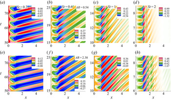
Figure 14 depicts the spatio–temporal response of  $v$ at a section
 $y=A/2$ on the
 $z=0$ plane in the streamwise direction for five shedding cycles. If we draw a horizontal line at a specified time, it intersects the wake at positive and negative values in an alternative manner. This clearly suggests highly coherent and periodic patterns of vortex structures across the streamwise extremes. We found a constant time lag between the shed vortices for a given
 $St$. An increase in
 $St$ generates additional time lags, and the maximum is noticed at
 $St=2$. Remarkably, the periodic vortex structures on the panel extent do not follow the
 $St$ dependence of the time lag, which starts beyond the trailing edge
 $(x>1)$ and end at the downstream wake. For
 $St=0.2$ and 0.6, a broadening of the cells is evident, indicating the growth of large-scale deformations associated with a vortex core flattening, this eventually imparts a stabilising influence on the near wake. In contrast, we observe streamwise diffusion of the cells for
 $St>1$. At
 $St=2$, we see that for
 $AR=0.54$, vortex structures mark their presence up to a location of
 $x\approx 3$. Beyond
 $x>3$, there is hardly any appearance of vertical velocities and, therefore, the corresponding absence of the wake vortices. This behaviour is attributed to the bifurcations of the primary vortex into a pair of transversely oriented twin-jet-type vortex trajectories. At
 $AR=2.38$, we observe a similar behaviour with an intermittent impression of high-frequency cells beyond
 $x>3$. This is attributable to the presence of multiple bifurcated structures comprising of swirling rings of vortices at
 $St=2$. Eventually, as the vortex structure becomes increasingly irregular with the downstream distance from the trailing edge, we observe the emergence of temporally correlated multiple velocity spots within the spatial regime
 $2\leqslant x\leqslant 3$.
Space–time reconstruction of the vertical velocity  $(v)$ in the streamwise direction at a vertical section
 $y=A/2$ on the midspan plane
 $z=0$. Note that while the
 $x$-axis represents the streamwise direction, the time evolution is displayed in the
 $y$ direction.

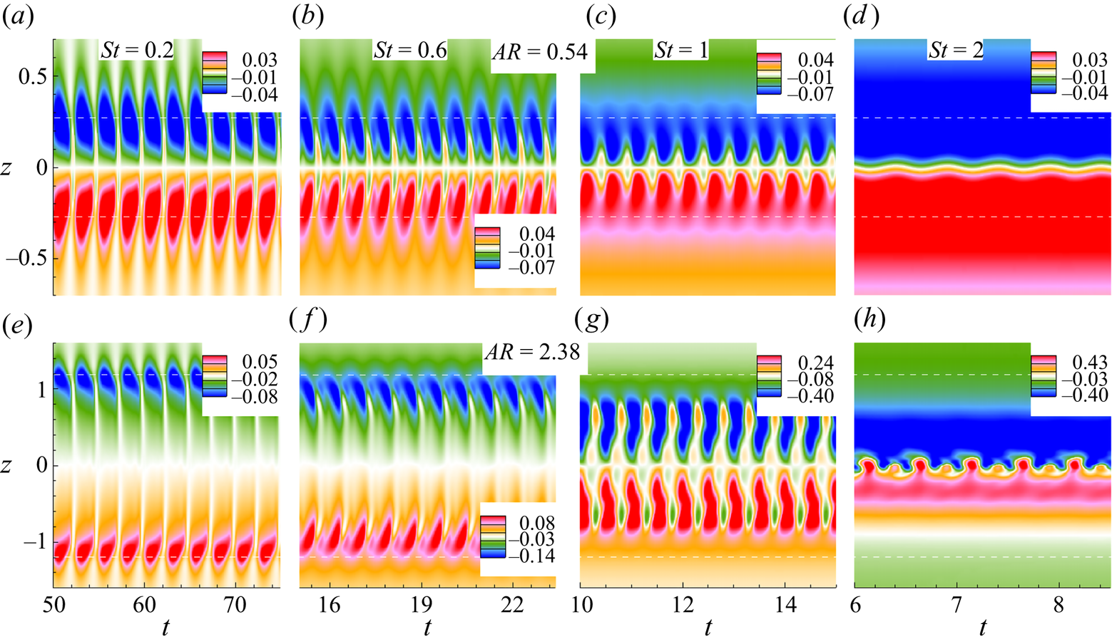
Along the span, figure 15 shows the temporal evolution of  $w$ velocity at a downstream section
 $x=1.5$ on
 $y=0$ plane for five vortex shedding cycles. We observe that the time-periodic negative and positive vortical structures symmetrically spanning across the positive and negative extremities of the panel about the
 $z=0$ plane. The core of the structures is positioned near the end of the panel, where the area occupied by the temporally correlated cells is more prevalent for
 $AR=0.54$. With increasing
 $St$, the growth of the secondary motion causes the spanwise cells to advance towards the central plane. Such narrowing down of the cells clearly highlights the signature of the wake compression. We further notice that structures are highly concentrated at the central plane for
 $AR=0.54$ at
 $St=2$ which show a periodic behaviour. At
 $AR=2.38$, we observe the formation of primary and secondary highly concentrated periodic cells restrained within a narrow band on either side of the central plane. Interestingly, we notice the occurrence of period doubling on the spanwise cells. Irrespective of
 $St$ and aspect ratio, the space–time reconstruction results of the streamwise cells in figure 14 shows five periods in as many shedding cycles. In contrast, the corresponding behaviour for the spanwise cells in figure 15 yield a doubling of the periods. To our knowledge, this period-doubling behaviour of the spanwise cells is probably the first demonstration for low-aspect-ratio pitching panels. We attribute this period-doubled response of the spanwise cells to the periodic formation of moderately distorted spanwise vortex structures and more complex structures characterised by the vortex rollup of inclined helical structures.
Space–time reconstruction of the spanwise velocity  $(w)$ along the span at a downstream section
 $x=1.5$ on the mid-vertical plane
 $y=0$. Note that while the
 $y$-axis represents the span, the time evolution is displayed in the
 $x$ direction.

3.5. Wake vortex interactions
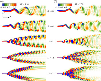
Figure 16 shows the streamwise interactions of the vortices through instantaneous  $\omega _z$ contours located at the
 $z=0$ plane for various
 $St$ and aspect ratio. We observe that for increasing
 $St$, vortical structures show two transitions with three independently distinct wake patterns. In the regime,
 $0.2\leqslant St\leqslant 0.6$, a pair of oscillating shear layers emerged from the panel with the tip connecting the leading edge, which roll up into horseshoe and bow-shaped vortices for
 $AR=0.54$ and
 $AR=2.38$, respectively. The wake does not resemble any discrete vortex structures from the side, usually characterised by elongated strands of negative and positive vorticity. The flow constricts downstream of the trailing edge, producing a wake with an appearance of diffused packets of negative and positive vortex contrails. The formation length of the vortex contrail decreases with increasing
 $St$, and the wake shows more dense diffused structures.
Instantaneous 2-D vorticity contours in the  $x$–
 $y$ plane
 $(\omega _z)$ for different Strouhal numbers; (a) corresponds to
 $AR=0.54$ and (b) corresponds to
 $AR=2.38$.

For  $St=1$, the wake shows a clear signature of a reverse von Kármán vortex street for both aspect ratios. The longitudinal diffusion between the wake structures is less for
 $AR=0.54$. This signifies minimal interactions between the cross-stream vorticities as attributed to the chain of engulfed horseshoe vortex structures. As such, each horseshoe vortex constitutes combinations of closed-loop vortices bound together at the tip with branching out the legs that distribute along the length to evolve into a spanwise shear layer (Buchholz & Smits Reference Buchholz and Smits2008). As a result, the self-induction of the curved tips causes transverse wake expansion farther downstream. At
 $AR=2.38$, the shed vortices from the trailing edge maintain a clear pattern, displaying a periodic flow field up to
 $2C$ downstream length. Thereafter, it bifurcates into multiple alternately signed streamwise cells, resulting in a transverse wake expansion. It is to be noted that the transverse expansion is associated with spanwise wake compression owing to the mutual induction of counter-signed streamwise vortex pairs both at the bottom and top of the wake (Buchholz & Smits Reference Buchholz and Smits2008). Farther downstream, these streamwise cells undergo lateral diffusion to yield blurred wake patterns.
The wake splits for  $St\geqslant 1.25$, developing two independent jets of vortex structures. There, the mean wake is symmetrically placed about the wake centreline. The corresponding structures, constituting each train, resemble coherent cells of consecutive positive and negative vortex loops. The strength and orientation of the loops change with
 $St$. At
 $St=1.5$ and
 $2$, we observe an approximately
 $45^\circ$ phase difference between the structures, with respect to the axis of the panel. Interestingly, the angle between the bifurcated streamwise jets increases with increasing
 $St$ and results in an expansion of the wake width. A larger wake width leads to a stable central region, which opposes any interaction between the streamwise or cross-stream vortices. In contrast, at
 $AR=2.38$, a more complex flow structure is observed. The bifurcated wake constitutes randomly distributed complex vortex loops and vortex contrails interacting with each other. The complexities in the flow field are further aggravated by increasing the Strouhal number. At
 $St=2$, approximately
 $C/2$ downstream from the trailing edge, appearances of distorted vortex loops and entangled structures augmenting both streamwise and cross-stream interactions of the vortices are seen.
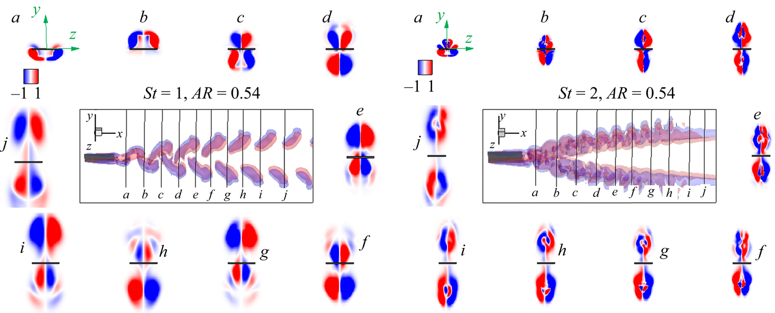
We analysed the vortex interactions with the instantaneous  $\omega _x$ contours at various transverse planes within the wake. Figure 17 shows that at
 $St=1$, plane
 $a$, which is located near to the trailing edge, contains counter-rotating pairs of the immediately shed horseshoe legs. Plane
 $(b)$ contains the tip of the horseshoe connected to plane
 $(a)$, which grows in size and strength with downstream distance. The interactions between the top and bottom horseshoes shed in the successive previous half cycles are seen in planes (c–e). We see leapfrog type interactions between the counter-rotating vortex pairs about the planes (c–e) (Buchholz & Smits Reference Buchholz and Smits2006). The plane
 $(f)$ contains the tip of the lowest horseshoe associated with plane
 $(e)$ and leg of the top horseshoe shed in the previous half period. The interaction pattern is similar to the one observed for planes (c–e). We notice similar repeated patterns in planes (g–j), where the vortices shed earlier than those in planes (c–f) for the consecutive four half-cycles. Notably, the distance between the cores of top and bottom vortex loops increases with increasing downstream distance from the trailing edge, resulting in weak cross-stream interactions. In contrast, the vortex interactions at
 $St=2$ shows merging and dissipation of vortex loops at various sectional planes (a–j). Plane (a), lying at the jet bifurcation zone, shows mutual interactions between the two most recently shed, oppositely oriented, tip and leg of the hairpin-like vortex structures. Plane (b) contains bifurcated structures, where vortices are seen to shed one pitching cycle earlier than those of plane (a). We observe vertical stretching of the vortex loops with increased strength and surface area. Additionally, there is spanwise merging of the cores at the symmetry axis
 $(z=0)$. In the subsequent planes (c–j), the vortex pairs grow in size with the merging of the core, leading to the emergence of secondary core-split structures.
Instantaneous planar view of streamwise vorticity contours  $(\omega _x)$ at various transverse planes (y–z) at
 $AR=0.54$ for
 $St=1$ (left panel) and
 $St=2$ (right panel). Interactions between vortices shown at cross-sectional planes (a–j) designate
 $1.2\leqslant {x}/{C}\leqslant 5.5$ with
 $\Delta x/{C}\approx 0.4$.

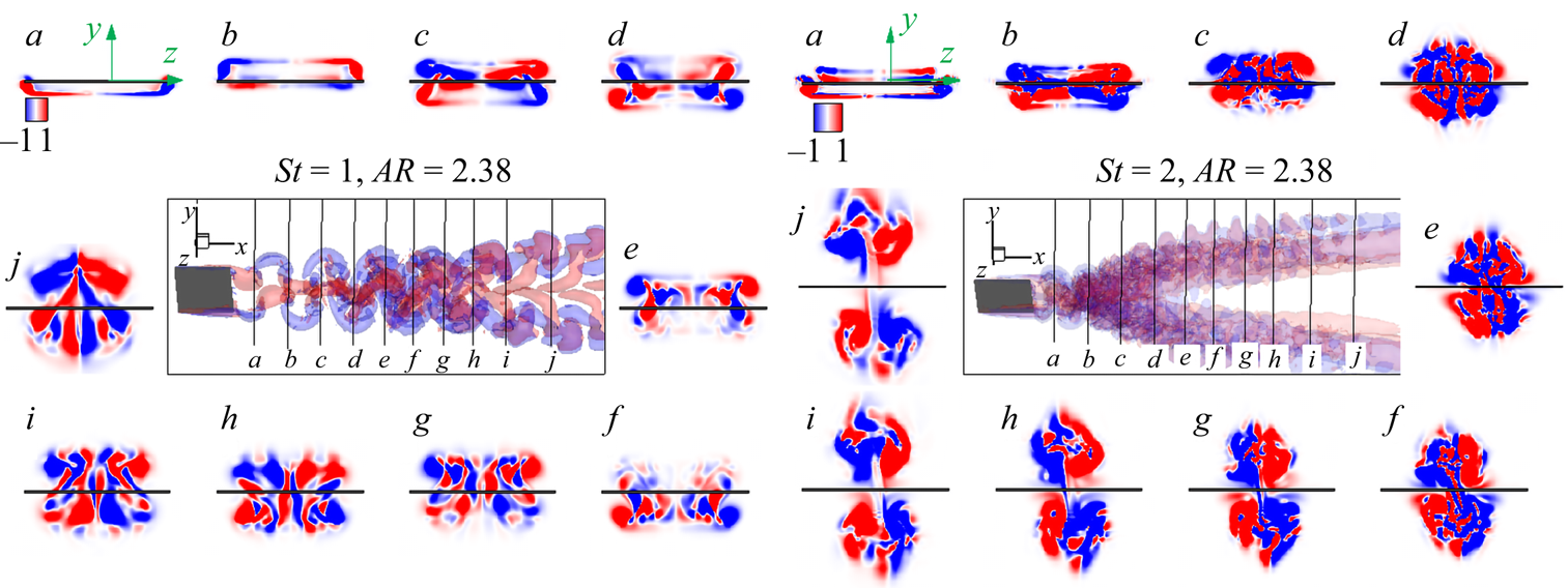
At  $St=1$ in figure 18, plane (a), near to the trailing edge shows the legs of immediately shed bow-shaped vortices. Plane (b) carries counter-signed vorticity loops consisting of the leg of the top vortex shed at the previous half-cycle and the tips of the immediately shed vortices. The complexities of the vortex interactions in the successive downstream planes (c–j) increase because of the complexities of the flow field. Again, owing to rapid cross-stream momentum exchange, the vortical loops across planes (c–j) undergo vortex merging, which increases with the downstream distance from the trailing edge. As a result, we observe the formation of vortex contrails of alternating sign. This is further exacerbated under the influence of the secondary instabilities. The evolution of new vortex couples and also the ensuing merging process is recurrent in planes (g–j). We observe from planes (a–j) that the structures have reflection symmetry about the
 $z=0$ plane marked by counter-rotating positive and negative vortex loops. Moreover, the maximum circulation strength is seen for the furthest plane
 $(j)$ with fewer cells covering the maximum area. In comparison, an alternate sign of chaotic structures spanning across the
 $y$–
 $z$ plane is seen at
 $St=2$. Apart from plane
 $(a)$, containing the leg of the instantly shed vortex, we cannot make any quantifiable information regarding primary vortex interaction patterns from planes (b–j). We notice accelerated cross-stream meandering interactions between multiple vortex loops for the downstream planes (b–f). For the planes (g–j), bifurcation in the wake disrupts cross-stream vorticity interactions and triggers localised interactions between the vorticity loops. It is possible that we see the formation of bridgelet-type vortex contrail connecting top and bottom vortices, located symmetrically about the plane
 $y=0$.
Planar view of instantaneous streamwise vorticity contours  $(\omega _x)$ at various transverse planes at
 $AR=2.38$ for
 $St=1$ (left panel) and
 $St=2$ (right panel). Vortex interactions are shown at cross-sectional planes (a–j) designate
 $1.2\leqslant {x}/{C}\leqslant 5.5$ with
 ${\Delta x}/{C}\approx 0.4$.

3.6. Force coefficients
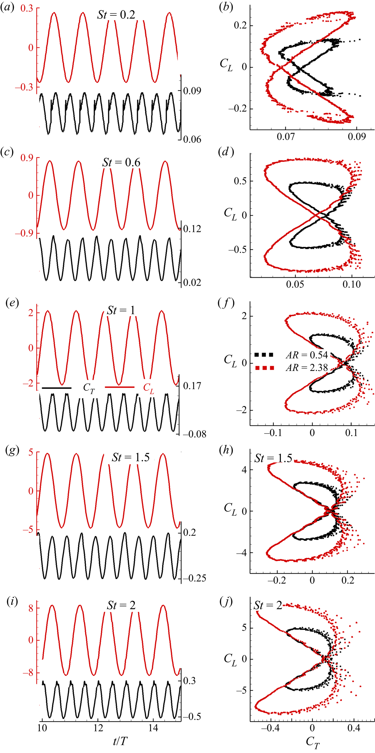
In figure 19, we show the time histories of  $C_T$ and
 $C_L$ for different
 $St$. In the right-hand panel, we show
 $C_T-C_L$ phase portraits for each
 $St$ and aspect ratio. This reveals that both
 $C_T$ and
 $C_L$ signals display a constant amplitude regular oscillations for the entire range of
 $St$. This essentially indicates periodic dynamics during the pitching motion. The panel experiences maximum thrust force just before it reaches pitching extremes and we notice that
 $C_T$ attains two peaks for all
 $St$ values. We find that the magnitude of
 $C_L$ is nearly twice that of
 $C_T$ (Dong et al. Reference Dong, Mittal and Najjar2006; Dai et al. Reference Dai, Luo, Ferreira de Sousa and Doyle2012). We attribute this observation to the larger amplitude of forced oscillations that exhibit stronger circulation in the shed vortices. It is found that the
 $C_T-C_L$ phase portraits reveal a closed attractor representing the periodic signature of the pitching motion. The phase portraits take the standard ‘8’-shaped loop where the crossover point is always located at
 $C_{L}=0$. Interestingly, for both aspect ratios, increasing
 $St$ leads to the gradual movement of the crossover point towards the positive
 $C_T$ axis, thereby causing the phase portrait to undergo a flip-flop transition. At
 $St\geqslant 1$, the crossover point ceases its movement, and the phase portrait resembles a mirror-image symmetry similar to the one for
 $St=0.2$. For all
 $St$, there is a significant enhancement in the force coefficients with an increase in aspect ratio.
Time histories of the thrust  $(C_T)$ and lift
 $(C_L)$ coefficients for different Strouhal numbers, where
 $T=St^{-1}$. The corresponding
 $C_T-C_L$ phase portraits are shown in the right-hand panel.

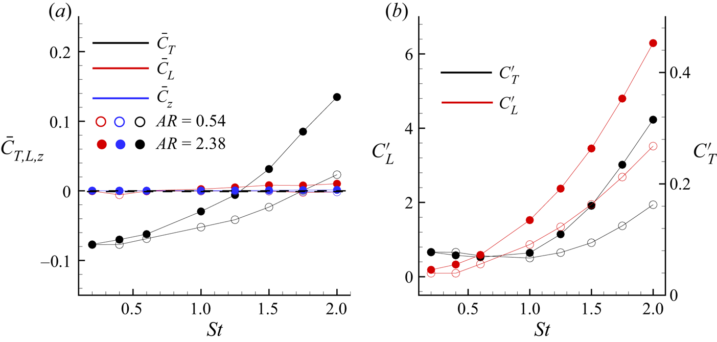
In figure 20(a), we plot the variation in the mean thrust  $(\overline {C_T})$, lift
 $(\overline {C_L})$ and spanwise force
 $(\overline {C_Z})$ coefficients as a function
 $St$ for
 $AR=0.54, 2.38$. We note that
 $\overline {C_T}$ increases monotonically with
 $St$, and that
 $\overline {C_T}$ is higher for larger aspect ratio, yielding a steeper
 $\overline {C_T}-St$ curve. We observe that a regime of negative
 $\overline {C_T}$ prevails for
 $St \lessapprox 1.2$ at
 $AR=2.38$, whereas the corresponding region at
 $AR=0.54$ is
 $St \lessapprox 1.7$. The streaming speed is the strong influencing parameter to yield negative
 $\overline {C_T}$ for these
 $St$ regimes, which becomes higher than the thrust produced by the panel. The results of negative
 $\overline {C_T}$ bear resemblance with the experimental results of Fernandez-Prats (Reference Fernandez-Prats2017) for a square rigid pitching panel. Moreover, the point of
 $\overline {C_T}=0$, indicating a symmetric
 $C_T$ signal about the
 $C_{T}=0$ axis, occurs at higher
 $St$ for decreasing aspect ratio. We found the zero mean thrust free-pitching condition for
 $(St)_{AR=0.54}\approx 1.75$ and
 $(St)_{AR=2.38}\approx 1.32$. Figure 20(a) also depicts that changes in
 $\overline {C_L}$ are insignificant with increasing
 $St$, and their values, although finite, are close to zero. This again demonstrates the symmetric nature of
 $C_L$ time signals for all
 $St$. For the present range of
 $St$, our computations show
 $F_z=0$, therefore, yielding
 $\overline {C_Z}=0$.
(a) Coefficient of mean thrust  $(\overline {C_T})$, mean lift
 $(\overline {C_L})$ and spanwise mean force coefficient
 $(\overline {C_Z})$ as a function of
 $St$ for different aspect ratios. (b) Variations of the r.m.s. thrust
 $(C_{T}^{\prime })$ and lift
 $(C_{L}^{\prime })$ coefficients with the Strouhal number for
 $AR=0.54$,
 $2.38$, respectively.

In figure 20(b), we show the variations of root-mean-squared  $(r.m.s.)$ thrust
 $(C_{T}^{\prime })$ and lift
 $(C_{L}^{\prime })$ coefficients with
 $St$ for
 $AR=0.54, 2.38$. The plot shows that both
 $C_{T}^{\prime }$ and
 $C_{L}^{\prime }$ increase with
 $St$ and aspect ratio, reaching a peak at
 $St=2$. We found that
 $C_{L}^{\prime }$ increases significantly with
 $St$, although
 $\overline {C_L}\approx 0$. However, the magnitudes of
 $C_{T}^{\prime }$ are significantly smaller
 $(O(10^{-1}))$ in contrast to
 $C_{L}^{\prime }$
 $(O(10))$. These enhancements in
 $C_{L}^{\prime }$ are attributed to the increased relative strengths of the horseshoe vortices and subsequent formations of the bifurcated jets at larger
 $St$. Furthermore, at
 $AR=2.38$, increasing
 $St$ causes the formation of multiple vortex contrails and a complex flow structure. The overall effect is a trigger in flow fluctuations and thereby increased magnitudes of
 $C_{L}^{\prime }$.
4. Conclusions
We performed numerical simulations of flow past a thin pitching panel of aspect ratio 0.54 and 2.38 placed in a uniform flow for  $Re=1000$. In particular, we have considered a wide range of
 $0.2 \leqslant St \leqslant 2$ to analyse the influence of pitching frequency on the 3-D vortex dynamics. Our computations show that within this range of
 $St$, the wake transition reveals vortex structures comprising horseshoe vortices at
 $St=0.6$, bow-shaped vortices, vortex rings, hairpin vortices at
 $St=1.75$, secondary bridgelets and large-tangled 3-D vortex structures for
 $St\geqslant 1.5$. We found a reverse von Kármán vortex street in the near wake for both aspect-ratio panels at
 $St=1$. An increase in
 $St>1$ reveals wake bifurcation into twin jets. At
 $AR=0.54$, the hairpin vortices transform into vortex rings, which start rotating at
 $St=2$. On the other hand, transverse asymmetrically bifurcated tangled vortices rolling over the isolated arrays of parallel strips are seen at
 $AR=2.38$.
We found that circulation strength increases with  $St$. The influences of aspect ratio and
 $St$ showed an increased spanwise movement of the flow. The flow converges towards the central region to yield wake compression at larger
 $St$. The wake compression is associated with a lower velocity magnitude at the central region than for the side wake. We found that the mechanism of the wake compression is attributable to the secondary instabilities driven by the spanwise pressure gradient, previously triggered by end effects. Streakline visualisations show a progressive growth in the wake width with increasing
 $St$. We found the formation of spokes at the shear-layer extremities for higher
 $St$, which become unstable earlier than the rest of the flow. The wake resembles a clear signature of conventional bluff-body motion at
 $AR=2.38$, resulting in a synchronised flow. Our results revealed the local nature of the three-dimensionality in the wake structures, and such localisation is higher at larger
 $St$.
The CWT at the midspan for  $AR=0.54$ at
 $St=2$ indicates a low-frequency band across the entire period, indicating periodic flow locked in with the pitching motion. The space–time behaviour in the streamwise direction reveals a constant time lag between the shed vortex structures for increasing
 $St$. At
 $AR=2.38$,
 $St=2$, we found irregular temporally correlated multiple velocity spots within the spatial regime
 $2\leqslant x\leqslant 3$. Interestingly, we have revealed the occurrence of period-doubling in the space–time behaviour of the spanwise cells.
The streamwise vortex interactions show that for  $St \leqslant 1$, the wake exhibits elongated strands of negative and positive vortices. Far downstream, the wake gives the appearance of diffused packets of negative and positive vortex contrails. The bifurcated jets found at
 $St \geqslant 1.25$ for
 $AR=0.54$ lead to an enhanced wake width, where the angle between the jets is found to increase with
 $St$. For
 $AR=2.38$, we found a chaotic signature in the wake constituting random interactions of vortex loops and vortex contrails. The
 $C_T-C_L$ phase portraits are found to behave as a closed attractor, which undergoes flip-flop transition with increasing
 $St$. The mean thrust coefficient increases monotonically with
 $St$ and aspect ratio. The r.m.s. thrust and lift coefficients show enhancement with
 $St$ and aspect ratio.
Acknowledgements
All the computations reported here were carried out on ‘Param-Ishan’, a 162-node 250 t.f.p.s. hybrid high-performance computing facility at IIT Guwahati.
Declaration of interests
The authors report no conflict of interest.