
1. Introduction
Electrohydrodynamics (EHDs) studies interactions between an electric field and a dielectric fluid of very low conductivity. This flow configuration has been widely applied in many industrial procedures. When an electric field is applied in thermoconvection flows, the thermal Nusselt number (ratio of convection to conduction, which quantifies the degree of heat transfer) will increase by up to an order of magnitude (McCluskey, Atten & Perez Reference McCluskey, Atten and Perez1991). The induced Coulomb force by the electric field can help create three kinds of EHD pumping, namely the induction pumping, ion-drag pumping and conduction pumping (Seyed-Yagoobi Reference Seyed-Yagoobi2005). In addition, the electric force can also be used to destabilise the interface between different liquids, improving the efficiency of mixing in the liquid–liquid system, which assists to step forward the design of EHD mixers (Jalaal, Khorshidi & Esmaeilzadeh Reference Jalaal, Khorshidi and Esmaeilzadeh2013). Therefore, understanding thoroughly the flow motions in EHD is important. One typical problem of EHD, which encompasses the essential flow dynamics under the electric field and is suitable for theoretical studies, is an electroconvective (EC) flow in a dielectric liquid. This EC flow is confined between two parallel plane electrodes (i.e. injector and collector) and subjected to a unipolar injection of charges generated by ion-exchange membranes. However, the EC flow is not fully understood, exemplified by a lack of understanding of the discrepancy between the theoretical and experimental linear instability criteria (with the theoretical value being larger than the experimental one, see below). In the following, we will first summarise the works on the linear stability analyses and bifurcation analyses of the EC flow and then discuss concisely the position of the current work in the literature.
1.1. Linear instability in electroconvective flows
The EC flows that are considered in this work refer to the convective motion induced by the potential difference applied to two plane electrodes covered by ion-exchange membranes (Lacroix, Atten & Hopfinger Reference Lacroix, Atten and Hopfinger1975). The linear instability in this flow was first studied by Atten & Moreau (Reference Atten and Moreau1972), and the diffusion effect of charges was often neglected because of their negligible effect on the current generation (to be discussed further below). The parameter that controls the flow instability/stability is called the electric Rayleigh number  $T$, which quantifies the strength of the electric field. When the charge injection is very weak (i.e.
 $C\ll 1$, where
 $C$ is a non-dimensional number quantifying the charge injection level), the linear stability criterion is dependent on the injection strength, namely
 $T_cC^2 \approx 220.7$. In the case of space-charge-limit injection (SCL when
 $C\rightarrow \infty$), the result indicated that the linear stability criterion
 $T_c \approx 160.75$. However, the linear stability criterion was experimentally estimated to be in a range of
 $T_c \approx 100 \pm 10$ (Lacroix et al. Reference Lacroix, Atten and Hopfinger1975; Atten & Lacroix Reference Atten and Lacroix1978, Reference Atten and Lacroix1979). Lacroix et al. (Reference Lacroix, Atten and Hopfinger1975) mentioned that the perturbations they introduced into the EC flows for the onset of convection were small, which eliminated the possibility that they have mistakenly taken the finite-amplitude disturbance as infinitesimal (however, we mention in passing that the amplitude of the disturbance needed to trigger subcritical convections does depend on how subcritical is the flow system, that is, a more subcritical system only needs smaller finite-amplitude disturbances to transition to turbulence). Atten & Lacroix (Reference Atten and Lacroix1978) clearly demonstrated the subcritical nature of EC flows with a hysteresis loop (their figures 4 and 5), with the following critical values of
 $T$ for a strong injection (
 $C=10$),
 \begin{equation} \left.\begin{gathered} \text{Theory:}\quad T_c\approx 161, \quad T_f\approx 110, \\ \text{Experiment:}\quad T_c \approx 100, \quad T_f \approx 90, \end{gathered}\right\} \end{equation}
where  $T_f$ is the threshold for the finite-amplitude solution, under which no such solution exists. Note that when the injection is weak (
 $C$ is small), the stability conditions change; and we will focus on discussing the values of
 $T_c$ in the SCL regime, for which the experimental result is far lower than that theoretically predicted. This disagreement may originate from the following (but not limited to) facts that: first, the charge diffusion effects were neglected in the theoretical analysis; second, subcritical mechanisms may be at play; third, some inherent imperfections in experiments were not correctly modelled by the equations. The first issue was addressed by Pérez & Castellanos (Reference Pérez and Castellanos1989) who reported a non-negligible effect of charge diffusion on the linear stability criterion, which decreases as the charge diffusion effect increases. The second issue was discussed by Zhang et al. (Reference Zhang, Martinelli, Wu, Schmid and Quadrio2015) who performed modal and non-modal stability analysis (linear subcritical energy growth) with the charge diffusion included in the governing equations. However, the authors found that the transient energy growth in EC is small, and thus concluded that this issue is unimportant in this matter. This urges us to consider the third factor aforesaid.
The imperfections in the experiments may result in mismatch between theoretical modelling and experimental conditions. The imperfections we are going to discuss and model are those in the ion-exchange membranes, which include different degrees of, e.g. non-uniformity, morphology, surface unevenness, unclearness/fouling, all of which can to some extent result in local clustering of the ions generated, thus leading to a non-uniform or inhomogeneous charge injection; however, in the theoretical modelling, a homogeneous ion-injection mechanism is conventionally assumed. In the experiments of EC flows, e.g. in the papers by Lacroix et al. (Reference Lacroix, Atten and Hopfinger1975), Atten & Lacroix (Reference Atten and Lacroix1978), typically two planar or circular electrodes were covered with ion-exchange membranes, with one electrode serving as an ion injector and the other as collector. AMF A 60 was mainly used; but occasionally, metal plated and varnished glass electrodes were also used. These authors reported that a strong and reproducible injection of ions into polar liquids could be achieved. Although they have paid special attention to the purification of the tested liquid, they did not mention the possibility of imperfections in their ion-exchange membranes used or discuss its effect. On the other hand, the ion-exchange materials are prone to be spatially non-uniform, even in the advertised homogeneous membranes and gel ion-exchangers (Zabolotsky & Nikonenko Reference Zabolotsky and Nikonenko1993). In fact, in the community of membrane science, reporting and studying the imperfections in the membrane are important and necessary (Selvey & Reiss Reference Selvey and Reiss1985; Vrijenhoek, Hong & Elimelech Reference Vrijenhoek, Hong and Elimelech2001; Tanaka Reference Tanaka2015) as the non-uniformity/morphology/fouling in the membrane is detrimental and inevitable (to some degree). In the context of EC flows, this non-uniformity of ion-exchange membranes may affect the physical and chemical properties of ion-exchange systems and the subsequent fluid motions driven by the Coulomb force therein. For a more detailed discussion on the inhomogeneity on the ion-exchange membranes, the reader is referred to Appendix A, where we also mention an early EHD experiment where ion-exchange membranes were not used and the authors found that the linear criteria between theory and experiment matched each other. These imperfections in the experiments involving ion-exchange membranes (Lacroix et al. Reference Lacroix, Atten and Hopfinger1975; Atten & Lacroix Reference Atten and Lacroix1978) may result in mismatch between theoretical modelling and experimental conditions. However, in theoretical and numerical studies, as we just mentioned, for the sake of simplicity, homogeneous injections and electric potential are conventionally assumed with an untested understanding that such simplification will not exert a significant influence on the results. In this work, we will study the effect of the inhomogeneity in the ion-injection mechanism, which results from the aforementioned imperfections in the ion-exchange membrane, by using stochastic bifurcation analyses. In the following, we review works on deterministic and stochastic bifurcation analyses of convective flows.
1.2. Bifurcation and chaos in electroconvective flows
After the emergence of electroconvective flows, as the strength of the electric field further increases, various successive flow bifurcations can take place, such as periodic (i.e. Hopf bifurcation), quasi-periodic and even chaotic motions. The first bifurcation in EC flows is subcritical (Félici Reference Félici1971; Lacroix et al. Reference Lacroix, Atten and Hopfinger1975; Zhang Reference Zhang2016), which is characterised by an abrupt jump in the strength of flow motion from zero to a finite value when finite-amplitude perturbations are present. For this subcritical bifurcation,  $T$ is larger than
 $T_f$ (i.e. nonlinear stability criterion for the finite-amplitude solution. When
 $T< T_f$, finite-amplitude perturbation cannot trigger flow motion) and smaller than
 $T_c$. For infinitesimal perturbations, only the supercritical transition route is possible, i.e. the required value of
 $T$ for flow motion should be larger than
 $T_c$. That
 $T_f$ is smaller than
 $T_c$ manifests a hysteresis loop, which is a unique feature of subcritical systems.
The chaotic characteristics of EC flows have been confirmed in some experiments. In the case of strong unipolar injection in confined circular boxes, the EC flow became time-dependent and chaotic above the instability threshold (Atten, Lacroix & Malraison Reference Atten, Lacroix and Malraison1980). Such a phenomenon has been observed for all aspect ratios ranging from approximately 2 up to 30 in their experiment, and one characteristic frequency and its subharmonic were found in the power spectra of the total current fluctuations. This characteristic frequency may originate from an oscillatory instability of the basic convection in each cell as it shows similar frequency with the normal velocity component. Malraison & Atten (Reference Malraison and Atten1982) found two types of chaotic behaviours in the power spectra of the intensity fluctuations, namely the exponential decay in the viscous-dominated flow and a power-law decay in the inertially dominated flow. Furthermore, the trajectories in a  $n$-dimensional phase space have been reconstructed based on the experimentally obtained time series of the total current fluctuations with a time-delay technique (Malraison et al. Reference Malraison, Atten, Berge and Dubois1983), then the fractal dimension of chaotic attractor was calculated based on the Grassberger–Procaccia method (Grassberger & Procaccia Reference Grassberger and Procaccia1983). In this problem of strong unipolar injection with an external voltage
 $U=270\ \textrm {V}$ in a dielectric liquid (critical voltage
 $U_c\simeq 50\ \textrm {V}$) confined in a cylindrical container of aspect ratio
 $\varGamma \approx 1$, the corresponding fractal dimension was estimated as
 $5.1 \pm 0.3$, which indicates that the attractor is of a strange type. However, this method becomes inapplicable when the logarithm of the integral correlation function does not show a defined slope. In such a case, Atten et al. (Reference Atten, Caputo, Malraison and Gagne1984) concluded that the fractal dimension seems to increase without limit. For the thermal convection, or Rayleigh–Bénard convection (RBC, which has also been studied by Malraison et al. Reference Malraison, Atten, Berge and Dubois1983), its dimension of strange attractor is approximately
 $2.8\pm 0.1$ under conditions
 $Pr=40$,
 $Ra/Ra_c=235$ and aspect ratios
 $\varGamma _x=2$,
 $\varGamma _y=1.2$ in a rectangular container (where
 $Pr$ is the Prandtl number quantifying the ratio between momentum diffusivity to thermal diffusivity and
 $Ra$ is the Rayleigh number in thermal convection measuring the relative strength between buoyancy and viscosity). In a larger container
 $\varGamma _x=\varGamma _y=2$ with parameters
 $Pr=1$ and
 $Ra=2\times 10^4$, the dimension of chaotic attractor for thermal convection is found to be
 $3.3$ with two positive and one possibly zero Lyapunov exponents (Urata Reference Urata1987; Castellanos Reference Castellanos1990).
In addition to the aforementioned experiments, the chaotic nature of EC flow has also been investigated in numerical simulations. By extracting time series from numerical simulations, Chicón, Pérez & Castellanos (Reference Chicón, Pérez and Castellanos2001) calculated the largest Lyapunov exponents to evidence the chaos in the EC flow with weak injection (i.e.  $C=0.1$). After constructing an
 $m$-dimensional phase space
 $s_n$ from time series, they applied the algorithm proposed by Kantz & Schreiber (Reference Kantz and Schreiber2004) to obtain a linear function
 $S(\Delta n)$ whose coefficient of proportionality was the desired largest Lyapunov exponent. Their work not only verified the emergence of chaos by positive largest Lyapunov exponents, but also indicated that the largest Lyapunov exponent is an increasing function of the average amplitude of the velocity, which means that the system became more and more chaotic as the liquid velocity increases. Near the nonlinear criterion of chaos, they also found that the largest Lyapunov exponent is quite small and the dimension of strange attractor may be smaller than
 $5$. However, their algorithm of computing Lyapunov exponents only works well when the embedding dimension
 $m$ is enough to support the attractor; otherwise, the Lyapunov exponent estimated from the linear part of
 $S(\Delta n)$ usually decreases when this dimension
 $m$ is increased. In addition, their numerical simulations focused on the regime of weak injection, while the strong injection case will be studied in the current work.
In the former literature on electroconvection, the estimation of Lyapunov exponent and the fractal dimension for electroconvective flow was based on the time series obtained from experiments and numerical simulations, but in these algorithms some free parameters must be introduced such as the embedding dimension and delay time. To characterise the chaotic motions in EC flows in a more systematic way and avoid assigning free parameters, we will follow the method of Wolf et al. (Reference Wolf, Swift, Swinney and Vastano1985), which has the capacity to compute multiple Lyapunov exponents. In this method, the Lyapunov spectrum is obtained by constructing multiple trajectories in the phase space, and these trajectories are evolved by solving the nonlinear and linear governing equations simultaneously. After obtaining the Lyapunov spectrum, the fractal dimension of attractor can be estimated from the well-known Kaplan–Yorke formula (Kaplan & Yorke Reference Kaplan and Yorke1979). The estimation of Lyapunov exponents based on this method has been widely applied in the study of chaos in RBC (Egolf & Greenside Reference Egolf and Greenside1994; Egolf et al. Reference Egolf, Melnikov, Pesch and Ecke2000; Paul et al. Reference Paul, Einarsson, Fischer and Cross2007; Levanger et al. Reference Levanger, Xu, Cyranka, Schatz, Mischaikow and Paul2019), but not so in electroconvection. Their results have revealed that the dynamics in thermal convection is truly chaotic as illustrated by a positive leading-order Lyapunov exponent and that the chaos in RBC is extensive over a range of finite-sized systems indicated by a linear scaling between the Lyapunov dimension of the chaotic attractor and the system size. In large chaotic systems, the Lyapunov dimension was first conjectured to be extensive by Ruelle (Reference Ruelle1982). Such extensive characteristic indicates the weak coupling between different subsystems if they are extracted from the same chaotic system, and these subsystems contribute additively to the overall fractal dimension (Eckmann & Ruelle Reference Eckmann and Ruelle1985); namely the summation of Lyapunov dimensions for each subsystem refers to the Lyapunov dimension of overall system.
The above paragraphs review the results of deterministic bifurcations of EC flows with some possible improvement areas being identified. A stochastic bifurcation analysis, on the other hand, has not been performed for EC flows. As discussed above, the stochastic bifurcation analysis may be used to model the imperfections in the experiments, to some degree. Such stochastic effects have been investigated in the case of RBC. Venturi, Wan & Karniadakis (Reference Venturi, Wan and Karniadakis2010) studied the stochastic bifurcation and stability of RBC within two-dimensional (2-D) square enclosures. They took into account two different sources of uncertainty. One source of uncertainty is represented by the random  $Ra$, the range of which includes the onset value for convective instability. The other source of uncertainty is the random initial conditions which can eventually induce different convection patterns. Their results indicated that the most probable convection pattern which develops from a low-wavenumber initial state is a one-roll pattern. Furthermore, Venturi, Choi & Karniadakis (Reference Venturi, Choi and Karniadakis2012) also considered stochastic temperature distribution at solid boundaries subjected to non-uniform unpredictable perturbations to mimic the realistic boundary conditions in thermal convection problems. In such a case, the bifurcation process leading to convection cannot provide a critical
 $Ra$ because convection occurs for most Rayleigh numbers (Ahlers, Meyer & Cannell Reference Ahlers, Meyer and Cannell1989), and the pure conduction state no longer exists, being replaced by a quasi-conduction regime (Kelly & Pal Reference Kelly and Pal1978). Motivated by their works, we will in this work apply the stochastic bifurcation analysis to the EC flows to study the effects of stochasticity added into the boundaries of electric potential and charge injection.
1.3. The position and structure of the current work
To sum up, after reviewing the above works, we realise that the deterministic bifurcation analysis of EC flows can be further refined by using a more systematic approach and the stochastic bifurcation analysis can be used to study and model the inevitable non-uniformity of the ion-exchange membrane in EHD experiments. By doing so, the position of the current work is clear: we will obtain more methodical results regarding the chaos in EC flows and also investigate to what extent the assumption of homogeneous injection and electric potential on electrodes can influence the theoretical results on the flow stability and bifurcation in EC flows. This will help to forge part of a plausible explanation in resolving the long-standing discrepancy of linear stability criteria between the experiment and theory.
The paper is organised as follows. In § 2, we introduce the configuration of electroconvective flows, the nonlinear governing equations and their corresponding linearisation around the base flow, the deterministic and stochastic boundary conditions, as well as the numerical method. In § 3, the numerical code is validated against existing results in the literature. Our results concerning the bifurcations of EC flows are analysed, which includes the deterministic and stochastic bifurcation analyses. Finally, in § 4, we summarise our conclusions and discuss possible future works.
2. Problem formulation and numerical method
2.1. Mathematical modelling
We consider a dielectric liquid confined between two parallel planar electrodes separated by a distance  $H^*$ and with a length
 $L^*$ in an
 $x$–
 $y$ plane (see figure 1), where the superscript asterisk
 $^*$ denotes dimensional variables. Because we focus on the linear criticality and primary bifurcations, it is appropriate to study 2-D EC flows in this work. The DC voltage difference between the top and bottom electrodes is given as
 $\Delta \phi _0^*$. Autonomous unipolar charges are generated through electrochemical reactions (Alj et al. Reference Alj, Denat, Gosse, Gosse and Nakamura1985) and are injected into a dielectric fluid from the bottom electrode with the charge density
 $Q_0^*$. In the current work, this dielectric liquid is assumed to be incompressible, Newtonian, isothermal and homogeneous. The governing equations consist of the incompressible Navier–Stokes equations and a reduced set of Maxwell's equations where the magnetic field is neglected owing to the low electric conductivity of the dielectric liquid, and only the Coulomb force is considered to be exerted on the fluid of constant permittivity
 $\epsilon ^*$ and viscosity
 $\mu ^*$. For the non-dimensionalisation, the length is non-dimensionalised by
 $H^*$, electric potential by
 $\Delta \phi _0^*$, charge density by
 $Q_0^*$, electric field
 $\boldsymbol {E}^*$ by
 $\Delta \phi _0^*/H^*$, velocity by the ionic drift velocity
 $K^*\boldsymbol {E}^*$ (i.e.
 $K^*\Delta \phi _0^*/H^*$), where
 $K^*$ is the ionic mobility, time by
 $H^{*2}/(K^*\Delta \phi _0^*)$ and finally pressure by
 $\rho _0^*K^{*2}\Delta \phi _0^{*2}/H^{*2}$. This yields the non-dimensional EHD equations as follows:
 $$\begin{gather} \nabla ^2 \phi ={-}CQ \end{gather}$$
 $$\begin{gather}{\boldsymbol{E}} ={-}\boldsymbol{\nabla} \phi \end{gather}$$
 $$\begin{gather}\frac{\partial Q}{\partial t} + \boldsymbol{\nabla} \boldsymbol{\cdot} [({\boldsymbol{E}}+{\boldsymbol{U}})Q] = \frac{1}{Fe}\nabla ^2 Q \end{gather}$$
 $$\begin{gather}\boldsymbol{\nabla} \boldsymbol{\cdot} {\boldsymbol{U}} = 0 \end{gather}$$
 $$\begin{gather}\frac{\partial {\boldsymbol{U}}}{\partial t} + ({\boldsymbol{U}} \boldsymbol{\cdot} \boldsymbol{\nabla}){\boldsymbol{U}} ={-}{\boldsymbol{\nabla}} P+ \frac{M^2}{T}\nabla ^2 {\boldsymbol{U}}+CM^2 Q {\boldsymbol{E}} \end{gather}$$
where
 \begin{equation} M=\frac{(\epsilon^*/\rho_0^*)^{1/2}}{K^*},\quad T=\frac{\epsilon^*\Delta \phi_0^*}{K^*\mu^*}, \quad C=\frac{Q_0^*H^{*2}}{\Delta \phi_0^* \epsilon ^*}, \quad Fe=\frac{K^*\Delta \phi_0^*}{D_{\nu}^*}. \end{equation}
The first parameter  $M$ denotes the ratio between the hydrodynamic mobility
 $(\epsilon ^*/\rho _0^*)^{1/2}$ and the ion mobility
 $K^*$. It is less than 0.1 for gases but larger than 1 for liquids (Castellanos & Agrait Reference Castellanos and Agrait1992). The electric Rayleigh number
 $T$ represents the ratio of the Coulomb force to the viscous force, which plays a similar role as the Rayleigh number
 $Ra$ in RBC. The
 $C$ measures the injection strength of charges. Here,
 $C\gg 1$ refers to the strong-injection regime (including the SCL) and
 $C\ll 1$ to the weak-injection regime. In the current work, we only consider the strong-injection regime as this is easier to realise in experiments and the linear criterion that we are going to investigate pertains to this regime. Finally,
 $Fe$ is the reciprocal of the charge diffusivity coefficient. A more detailed discussion of the above EHD equations and parameters can be found in the literature (Castellanos Reference Castellanos1998; Zhang et al. Reference Zhang, Martinelli, Wu, Schmid and Quadrio2015).
Schematic of stochastic perturbations  $g_i(x)$ on bottom and top plates with perturbation amplitude
 $\sigma =10\,\%$ and two different correlation lengths. Solid line,
 $l_c=1.0$; dash–dotted line,
 $l_c=0.25$. Smaller correlation length can induce more wavy oscillations. The two dashed ellipses refer to the electroconvective flow within the dielectric liquid. Stochastic boundaries may induce asymmetric motions.

We now discuss the boundary conditions for field variables  $\boldsymbol {U}=(U,V,W)$,
 $Q$ and
 $\phi$. In the current work, the deterministic and stochastic bifurcations are studied under different boundary conditions. In the deterministic case, the boundary conditions in the vertical direction are given as
 $$\begin{gather} y=0: \ \boldsymbol{U}=0, \, Q=1, \, \phi=1; \end{gather}$$
 $$\begin{gather}y=1: \ \boldsymbol{U}=0,\, \partial Q/\partial y=0, \, \phi=0. \end{gather}$$
If we consider (2.1) plus the above boundary conditions and assume homogeneity in wall-parallel directions, we can see that the system has the equivalence that  $(y,v,E_y) \rightarrow (1-y,-v,-E_y)$, where
 $E_y$ is the
 $y$ component of the electric field. This equivalence indicates that the injection from the top plate is the same as the injection from the bottom plate. In the current work, we consider the injection from the bottom.
Because in the current work the computational domain is finite in the lateral direction, we also need to specify boundary conditions on the lateral walls. Two choices for the velocity fields are considered, namely the no-slip (i.e.  $\boldsymbol {U}=0$) and periodic boundaries. They are used for different purposes: with the no-slip boundary condition, we can study the EC flow in finite domains of different aspect ratios with
 $\partial Q/\partial x=0$ and
 $\partial \phi /\partial x=0$ as the lateral boundaries of charge density and electric potential; under the periodic boundary conditions, the bifurcation of EC flows between two infinite parallel plates can be investigated. Note that in Appendix B, we also present the results of symmetric boundary conditions applied on the lateral walls to compare our results with those in the literature.
Owing to the inhomogeneity of ion-exchange membranes and their resistance on the transport of ions, inhomogeneous potential differences and charge injection can be induced on the membrane surface. In our study, these effects will be modelled by adding three spatially random perturbations  $g_1(x)$,
 $g_2(x)$ and
 $g_3(x)$ into the Dirichlet boundary conditions of charge density
 $Q$ and electric potential
 $\phi$, namely
 $Q(0)=1+g_1(x)$,
 $\phi (0)=1+g_2(x)$ and
 $\phi (1)=g_3(x)$, whose schematic is shown in figure 1. The above perturbations are quantified by two parameters, which are
 $\sigma$ as the maximum amplitude of the perturbation (with respect to the normalised boundary conditions) and
 $l_c$ as the correlation length normalised by the streamwise length
 $L$. One can also assign different values of
 $\sigma$ to different variables, but because we have considered normalisation in the boundary conditions and owing to the space limit, this parametric study will not be conducted in this work. These perturbations are designed to have a zero mean in the streamwise range
 $x\in [0,L]$, and they also follow the Gaussian correlation function (following Venturi, Wan & Karniadakis Reference Venturi, Wan and Karniadakis2008; Venturi et al. Reference Venturi, Choi and Karniadakis2012):
 \begin{equation} \langle g_i(x_1) g_i(x_2) \rangle = \sigma^2 \exp\left({ -A\frac{(x_1-x_2)^2}{L^2 l_c^2} }\right) , \end{equation}
where  $\langle \cdot \rangle$ denotes the ensemble average and
 $A$ refers to the normalisation constant. To eliminate the correlation between
 $g_i(x_1)$ and
 $g_i(x_2)$ at the distance of correlation length, here the normalisation constant is chosen to be
 $A=6$. Based on the Karhunen–Loève theorem and spectral analysis of (2.4), a stochastic process can be represented by a linear combination of orthogonal bases,
 \begin{equation} g_i(x)=\sigma \sum_{k=1}^{N_g} \langle b_k^2 \rangle^{1/2}\xi_k^{(i)}\psi_k(x),\quad i=1,2,3 , \end{equation}
where  $N_g$ refers to the dimensionality of series expansion,
 $\xi _k^{(i)}$ are zero-mean uncorrelated Gaussian random variables with unit variance and the orthogonal basis
 $\psi _k(x)$ is given as
 $\psi _0(x)=1$,
 $\psi _k(x)=\sqrt {2} \cos (2k{\rm \pi} x/L + \xi _k^0)$, which satisfy the periodic boundary condition along the streamwise direction. From the above (2.4) and (2.5), the covariance of
 $g_i(x)$ can be obtained:
 \begin{equation} C(x_1,x_2) = \frac{\langle g_i(x_1) g_i(x_2) \rangle}{\sigma^2} = \exp\left({ -6\frac{(x_1-x_2)^2}{L^2 l_c^2}}\right) = \sum_{k=1}^{N_g} \langle b_k^2 \rangle \psi_k(x_1)\psi_k(x_2) . \end{equation}
Thus, the positive Fourier coefficients  $\langle b_k^2 \rangle$ can be obtained by projecting this Gaussian covariance
 $C(x_1,x_2)$ onto the basis
 $\{ \psi _k(x)\}$,
 \begin{equation} \langle b_k^2 \rangle = \int_0^{L} \int_0^{L} C(x_1,x_2)\psi_k(x_1)\psi_k(x_2)\,\textrm{d}x_1\,\textrm{d}x_2. \end{equation}
With the above definitions of stochastic perturbations  $g_i(x)$, the boundary conditions in the stochastic bifurcation analysis read:
 $$\begin{gather} y=0: \ \boldsymbol{U}=0, \, Q=1+g_1(x), \, \phi=1+g_2(x); \end{gather}$$
 $$\begin{gather}y=1: \ \boldsymbol{U}=0, \, \partial Q/\partial y=0, \, \phi=g_3(x); \end{gather}$$
 $$\begin{gather}x=0 \ \& \ x=L:\ \text{periodic boundary}. \end{gather}$$
As mentioned above, because 2-D EC flows are to be studied here, but the non-uniformity in the ion-exchange membranes in reality is inherently three-dimensional (3-D), the results shown below should be interpreted with a local significance related to either one  $x$–
 $y$ slice in 3-D EC flows or the non-uniformity has a larger length scale in the
 $z$ direction than the 2-D EC flow structures we consider here. We mention in passing that the stochastic bifurcation analyses in Venturi et al. (Reference Venturi, Wan and Karniadakis2010, Reference Venturi, Choi and Karniadakis2012) were also 2-D.
2.2. Linearisation and stability analysis
The first bifurcation can be studied using a linear stability analysis. The linearised governing equations are obtained by decomposing the field variable into a sum of base state and perturbation, i.e.  $\boldsymbol {U}=\bar {\boldsymbol {U}}+\boldsymbol {u}$,
 $P=\bar {P}+p$,
 $\boldsymbol {E}=\bar {\boldsymbol {E}}+\boldsymbol {e}$,
 $Q=\bar {Q}+q$ and
 $\phi =\bar {\phi }+\varphi$. After substituting the above decompositions into the governing equations (2.1), by subtracting from them the governing equations for the base states and neglecting the second-order terms, the linearised governing equations read:
 $$\begin{gather} \nabla^2 \varphi ={-}Cq \end{gather}$$
 $$\begin{gather}\boldsymbol{e} ={-}\boldsymbol{\nabla} \varphi \end{gather}$$
 $$\begin{gather}\frac{\partial q}{\partial t}+ \boldsymbol{\nabla} \boldsymbol{\cdot} [(\bar{\boldsymbol{E}}+\bar{\boldsymbol{U}})q+(\boldsymbol{e}+\boldsymbol{u})\bar{Q}] = \frac{1}{Fe}\nabla^2 q \end{gather}$$
 $$\begin{gather}\boldsymbol{\nabla} \boldsymbol{\cdot} \boldsymbol{u} = 0 \end{gather}$$
 $$\begin{gather}\frac{\partial \boldsymbol{u}}{\partial t}+(\boldsymbol{u} \boldsymbol{\cdot}\boldsymbol{\nabla})\bar{\boldsymbol{U}} + (\bar{\boldsymbol{U}} \boldsymbol{\cdot}\boldsymbol{\nabla}) \boldsymbol{u} ={-} \boldsymbol{\nabla} p + \frac{M^2}{T}\nabla ^2 \boldsymbol{u} + CM^2(q\bar{\boldsymbol{E}}+\bar{Q}\boldsymbol{e}). \end{gather}$$
For the linear stability analysis in deterministic and stochastic cases, the boundary conditions of perturbed fields are given as
 $$\begin{gather} y=0: \ \boldsymbol{u}=0, \, q=0, \, \varphi=0; \end{gather}$$
 $$\begin{gather}y=1: \ \boldsymbol{u}=0, \, \partial q/\partial y=0, \, \varphi=0; \end{gather}$$
 $$\begin{gather}x=0 \ \& \ x=L: \ \boldsymbol{u}=0, \,\partial q/\partial x=0, \, \partial \varphi/\partial x=0 \ \text{or} \ \text{periodic boundary}. \end{gather}$$
Some discussions on the difference between the deterministic and stochastic cases in the stability analysis are in order. The difference mainly lies in the different boundary conditions in the base flows to be used. In the deterministic case, the hydrostatic solutions to the governing equations are adopted as the base flow ( $\bar {\boldsymbol {U}}=0$ and steady solutions to Maxwell's equation with homogeneous boundary conditions, which is the common practice in the previous works). In the stochastic case, we also use
 $\bar {\boldsymbol {U}}=0$ for the velocity field but the steady solutions to Maxwell's equation with stochastic boundary conditions for the electric field as the base flow. Figure 2 shows the steady solutions of charge density with deterministic and stochastic boundary conditions. The variation of
 $\bar {Q}$ mainly locates around the bottom boundary (i.e.
 $y=0$). It can be understood that in the deterministic case, if the flow is unstable, the intrinsic nonlinearity mechanism in the equations is the only source for the nonlinear development in this flow; whereas in the stochastic case, if the flow is unstable, in addition to the intrinsic nonlinearity mechanism, the stochastic boundary conditions will serve as a catalyst to bring the flow to a nonlinearly saturated state more quickly (in a shorter time) or more easily (requiring a lower
 $T$). We will discuss this point further in § 3.
Hydrostatic solutions of charge density  $\bar {Q}$ for electroconvective flows in deterministic and stochastic cases with
 $C=10$ and
 $Fe=10^4$: (a) base field
 $\bar {Q}$ under deterministic boundaries; (b) base field
 $\bar {Q}$ under stochastic boundaries with
 $\sigma =2\,\%$ and
 $l_c=0.5$. Only part of the field
 $0< y<0.2$ is presented for a clear visualisation (the charge density in the range of
 $0.2< y<1$ is relatively small); (c) comparison of profiles for
 $\bar {Q}$ between deterministic (black line) and stochastic cases (grey lines, at 12 different
 $x$ stations, separated equally).

Based on the above non-dimensional perturbation variables, the total energy density in electroconvective flows can be defined by
 \begin{equation} \mathcal{E}=\mathcal{E}_k+\mathcal{E}_{\varphi}=\tfrac{1}{2}(\boldsymbol{u}^2+M^2\boldsymbol{e}^2), \end{equation}
where the perturbation velocity  $\boldsymbol {u}=(u,v,w)$ and electric field
 $\boldsymbol {e}=(e_x,e_y,e_z)$. The total energy in EC flow consists of kinetic energy
 $\mathcal {E}_k$ and the perturbed electric energy
 $\mathcal {E}_{\varphi }$. The latter follows the definition by Castellanos (Reference Castellanos1998) and has also been used by Zhang et al. (Reference Zhang, Martinelli, Wu, Schmid and Quadrio2015) and Zhang (Reference Zhang2016).
We now discuss the method for quantitative determination of linear stability criterion  $T_c$. We here use
 $T$ as the stability parameter. The above linear equations (2.9) can be rewritten in the following form:
 \begin{equation} \frac{\partial \boldsymbol{f}}{\partial t}=\boldsymbol{\mathcal{L}}\boldsymbol{f} , \end{equation}
where  $\boldsymbol {\mathcal {L}}$ refers to the linear evolution operator and
 $\boldsymbol {f}$ is the array for the perturbed variables in the above linear equations. When steady base states are considered, the small-amplitude perturbations can be assumed to take on wave-like shapes in time, thus they can be denoted by
 \begin{equation} \boldsymbol{f}(x,y,t)=\hat{\boldsymbol{f}}(x,y)\ \textrm{e}^{\omega t}, \end{equation}
where  $\omega =\omega _r+\textrm {i}\omega _i$,
 $\omega _r$ denotes the temporal growth rate of perturbations and
 $\omega _i$ is the phase speed. If
 $\omega _r$ is positive, the perturbations will grow in time and the system is unstable. After substituting the above expression of the linear perturbations into (2.12), the following eigenvalue problem can be obtained:
 \begin{equation} \omega \hat{\boldsymbol{f}} = \boldsymbol{\mathcal{L}}\hat{\boldsymbol{f}}. \end{equation}
Because we will consider a confined space in  $x,y$ directions (thus, the corresponding analysis becomes a global stability analysis, see Theofilis Reference Theofilis2011), we use the matrix-free method based on a time-stepping method (Edwards et al. Reference Edwards, Tuckerman, Friesner and Sorensen1994; Tuckerman & Barkley Reference Tuckerman and Barkley1999), where the action of the evolution operator on the perturbation vector can be implemented by integrating in time the linearised equations. In such a time-stepping technique, the Arnoldi algorithm is applied to extract the eigen-information in the linearised system by constructing a Krylov subspace using snapshots taken from the linear evolution of the perturbation vector. Based on our above definition of total energy density, here the perturbation vector only involves
 $\boldsymbol {u}$ and
 $\boldsymbol {e}$, and other variables can be readily computed from these two. To obtain better convergence and accuracy, the implicitly restarted Arnoldi method (IRAM) from the ARPACK library (Lehoucq, Sorensen & Yang Reference Lehoucq, Sorensen and Yang1998) is applied to solve the above eigenvalue problem. For linear stability analysis, the steady solution to the nonlinear equations (2.1), with either deterministic or stochastic boundary conditions, has been applied as the base state for the linear equations (2.9). Once enough data (3–4 data points) of the growth rates around
 $\omega _r=0$ for different stability parameters
 $T$ are obtained, the linear stability criterion can be calculated by a linear interpolation of the data to determine the value of
 $T_c$ at which
 $\omega _r=0$. Below, the results of the linear stability using the time-stepping Arnoldi method will be compared extensively with those of the linear stability analysis by Zhang et al. (Reference Zhang, Martinelli, Wu, Schmid and Quadrio2015) when the comparison is possible.
2.3. Lyapunov exponents and Lyapunov dimension
In the current work, we will additionally calculate the spectrum of Lyapunov exponents based on the governing equations of electroconvective flow by applying the algorithm proposed by Wolf et al. (Reference Wolf, Swift, Swinney and Vastano1985). A Lyapunov exponent characterises the rate of separation of a pair of initially infinitesimally close trajectories in a phase space. We choose the state vector  $\boldsymbol {H}_0=[\boldsymbol {U},\boldsymbol {E}]$ evolved by the nonlinear equations (2.1) as the reference trajectory. The other trajectory, evolving around the reference trajectory, is constructed by the state vector,
 $\boldsymbol {H}_k=\boldsymbol {H}_0+\boldsymbol {h}_k=[\boldsymbol {U}+\boldsymbol {u}_k,\boldsymbol {E}+\boldsymbol {e}_k]$
 $(k=1,2,\ldots ,m)$, where
 $m$ refers to the number of desired Lyapunov exponents (equivalently,
 $m$ pairs of trajectories with the common one being the reference trajectory aforementioned), and then the separated distance between
 $\boldsymbol {H}_0$ and
 $\boldsymbol {H}_k$ can be evaluated by the magnitude of corresponding perturbed vector
 $\boldsymbol {h}_k$ in the energy norm (2.11):
 \begin{equation} \left\| \boldsymbol{h}_k(\boldsymbol{x},t) \right\|=\sqrt{\frac{1}{V}\iint_V[\boldsymbol{u}_k(\boldsymbol{x},t)^2+M^2\boldsymbol{e}_k(\boldsymbol{x},t)^2]\,\textrm{d}x\,\textrm{d}y}. \end{equation}
Each perturbed vector is evolved by a set of linear equations (2.9) which adopt the state vector  $\boldsymbol {H}_0$ as the base field. In addition, to trace the fastest change of
 $\boldsymbol {h}_k$, a Gram–Schmidt procedure is repeatedly applied to the perturbed vectors at each
 $\Delta t$ interval. The instantaneous Lyapunov exponent for a continuous-time dynamical system is defined as the derivative of the logarithm of the divergence rate (Shin & Hammond Reference Shin and Hammond1998). Thus, its discrete form
 $\tilde {\lambda }_k^i$ at time
 $t^i$ can be calculated as
 \begin{equation} \tilde{\lambda}_k^i=\frac{1}{\Delta t}\ln \frac{\| \boldsymbol{h}_k(\boldsymbol{x},t^i+\Delta t) \|}{\| \boldsymbol{h}_k(\boldsymbol{x},t^i) \|}. \end{equation}
The above procedure is required to be repeated until the convergence of the finite-time Lyapunov exponent,
 \begin{equation} \lambda_k=\frac{1}{N_L}\sum_{i=1}^{N_L} \tilde{\lambda}_k^i, \end{equation}
where  $N_L$ is the total number of Gram–Schmidt orthonormalisations. The convergence criterion is the relative error between the
 $i$-th and
 $i+1$-th Gram–Schmidt procedures being less than
 $10^{-5}$.
As the perturbed vectors are orthogonal to each other after the Gram–Schmidt procedure, the summation of  $N_L$ Lyapunov exponents
 $\sum _{i=1}^{N_L} \lambda _i$ can describe the growth rate of a
 $N_L$-dimensional ball. Thus, the number of Lyapunov exponents that are summed to be zero corresponds to the dimension of this ball which will neither grow nor shrink, and this is the so-called Lyapunov dimension
 $D_{\lambda }$, which is the minimum number of active degrees of freedom that characterise the chaotic dynamics (Farmer, Ott & Yorke Reference Farmer, Ott and Yorke1983). After obtaining a sufficient number of Lyapunov exponents
 $\lambda _k$,
 $D_\lambda$ can be computed based on the Kaplan–Yorke formula: (Kaplan & Yorke Reference Kaplan and Yorke1979)
 \begin{equation} D_{\lambda}=K+\frac{S_K}{| \lambda_{K+1} |}, \end{equation}
where  $K$ is the largest
 $n$ for
 $S_n=\sum _{i=1}^n \lambda _i \geqslant 0$, namely
 $S_{K} \geqslant 0$ and
 $S_{K+1}<0$.
2.4. Numerical method
The direct numerical simulations (DNS) of electroconvection flows are performed using the computational fluid dynamics solver Nek5000 (Fischer, Lottes & Kerkemeier Reference Fischer, Lottes and Kerkemeier2008), which is based on the spectral element method (SEM) (Patera Reference Patera1984). It is well-known for its high accuracy, favourable dispersion properties and efficient parallelisation. This code has been widely used in the study of RBC (Paul et al. Reference Paul, Chiam, Cross, Fischer and Greenside2003; Sakievich, Peet & Adrian Reference Sakievich, Peet and Adrian2016) and other flows. In the current work,  $\mathbb {P}_{N}-\mathbb {P}_{N-2}$ formulation is applied for spatial discretisation; that is, the basis for the velocity space are
 $N$th-order Lagrange polynomial interpolants on Gauss–Lobatto–Legendre (GLL) points, while the pressure space is discretised using Lagrange interpolants of order
 $N-2$ defined on the Gauss–Legendre quadrature points. The polynomial order is set to 11 (i.e.
 $N=12$) for all following cases, thus, each spectral element is further discretised by
 $12\times 12$ GLL points. The second-order backward difference scheme (BDF2), coupled to a second-order extrapolation scheme (EXT2), is applied for time integration. The time step
 $\delta t$ is determined by the Courant–Friedrichs–Lewy (CFL) condition with the target Courant number being 0.15.
3. Results and discussions
3.1. Global linear instability (as a validation step)
In this section, we first present the results of the grid independency test and validation for the current EHD solvers. To facilitate the discussions below, we define an electric Nusselt number  $Ne$ (Traoré & Pérez Reference Traoré and Pérez2012; Zhang Reference Zhang2016), which reads:
 \begin{equation} Ne=\frac{I_e}{I_0}, \quad I_e=\iint_V \left[Q(V+E_y) - \frac{1}{Fe}\frac{\partial Q}{\partial y} \right]\textrm{d}x \,\textrm{d}y, \end{equation}
where  $I_e$ is the total current and
 $I_0$ refers to the total hydrostatic current when there is no fluid motion. Thus, the electric Nusselt number can be used to evaluate the efficiency of the transport of the electric current. Here, the charge diffusion has also been included to be consistent with our theoretical modelling above; but we did notice that its value is negligible compared with the other two ion-transport mechanisms. However, even though its contribution to
 $Ne$ is small, the charge diffusion has a non-negligible effect on the linear instability criterion and finite-amplitude solutions, as has been shown by Pérez & Castellanos (Reference Pérez and Castellanos1989), Zhang et al. (Reference Zhang, Martinelli, Wu, Schmid and Quadrio2015) and Zhang (Reference Zhang2016).
We now turn to the discussion of grid independence. Here the element size is used to represent different mesh resolutions, but it should be noted that each spectral element also contains  $12\times 12$ GLL points when computing the total number of grid points. For the electroconvective flow under periodic lateral boundaries, two element sizes, namely
 $12\times 16$ and
 $18\times 24$, have been tested with parameters
 $C=10$,
 $M=10$ and
 $Fe=10^4$. The time-averaged electric Nusselt numbers (i.e.
 $Ne_{avg}$) are computed for multiple electric Rayleigh numbers involving both the steady and chaotic cases. In the current work, steady and chaotic flow regimes are considered. In the former regime, the variation of the linear stability criterion is discussed, while chaotic characteristics of the EC flow are investigated in the latter regime. The results of grid independence are shown in table 1. It is found that the relative errors between element sizes
 $12\times 16$ and
 $18\times 24$ are all less than
 $1\,\%$. Therefore, the element size of
 $12\times 16$ is applied in the following numerical simulations considering both the accuracy and computational efficiency. For different geometry aspect ratios
 $\varGamma =L^*/H^*$, the number of elements in the normal direction remains constant, while the number of elements in the lateral direction increases with
 $\varGamma$. In addition, those elements close to the top and bottom planes have been refined. As the GLL quadrature cluster those grid points around the edge of elements, the resolution is further improved near the walls.
Grid independency test for electroconvective flows by time-averaged electric Nusselt numbers  $Ne_{avg}$ at different electric Rayleigh numbers
 $T$ within the domain range
 $[0,1.228]$ in the
 $x$ direction and
 $[0,1]$ in the
 $y$ direction.

At the first step of validation, we verify the calculation of the steady solution to the nonlinear equations (2.1) with deterministic boundary conditions. Under the condition of steady flow field  ${\boldsymbol {U}}=0$ (i.e. no fluid motion), the steady electric field depends only on the injection strength
 $C$ and the reciprocal of the charge diffusion coefficient
 $1/Fe$. Such a steady hydrostatic solution can also be obtained by directly solving for the steady solution to the electric governing equations (i.e. (2.1a–c) with
 ${\boldsymbol {U}}=0$), which can be easily obtained using an ordinary differential equation (ODE) solver, as done by Zhang et al. (Reference Zhang, Martinelli, Wu, Schmid and Quadrio2015). In figure 3, we use two levels of injection strength
 $C=10$ and
 $C=20$ for validating our numerical steady solutions by DNS against the results obtained by the ODE solver (Zhang et al. Reference Zhang, Martinelli, Wu, Schmid and Quadrio2015). At
 $C=10$, the difference is
 $0.080\,\%$ for
 $Q$ and
 $0.183\,\%$ for
 $E_y$ in terms of the root-mean-square error. At
 $C=20$, the root-mean-square error is
 $0.072\,\%$ for
 $Q$ and
 $0.186\,\%$ for
 $E_y$. Thus, these two results agree with each other quite well.
Validation of hydrostatic solutions of charge density  $Q$ and electric field
 $E_y$ for electroconvective flows at
 $M=10, Fe=10^4$ and two different injection strengths: (a)
 $C=10$; (b)
 $C=20$. Circle and square symbols refer to results of charge density and normal electric field from the current numerical simulations, and the solid line is obtained by an ODE solver solving the electric equations.

Next, the accuracy of simulating the dynamics in the nonlinear equations is tested by numerically evolving them to calculate the linear and nonlinear criteria. As we have discussed in the introduction section, there are two critical values of  $T$, i.e. linear criterion
 $T_c$ and finite-amplitude (or nonlinear) criterion
 $T_f$. We will calculate their values at
 $C=10, M=10$ and
 $Fe=10^4$. The periodic boundary condition is applied on the lateral walls. The spatial length in the
 $x$ direction is
 $L=1.228$, which corresponds to the wavelength of the least stable mode in the linearised EC flow at these parameters (Atten & Moreau Reference Atten and Moreau1972; Zhang et al. Reference Zhang, Martinelli, Wu, Schmid and Quadrio2015).
Figure 4 shows the relation between the electric Nusselt number  $Ne$ and the electric Rayleigh number
 $T$ with a hysteresis loop. The two stability criteria are numerically obtained as
 $T_c=162.5$ and
 $T_f=110.4$. This linear stability criterion agrees very well with that predicted by the stability analysis approach
 $T_c=162.6$ (Zhang et al. Reference Zhang, Martinelli, Wu, Schmid and Quadrio2015). Under the symmetric lateral boundary conditions (with the computational length
 $L=0.614$) and parameters
 $M=10$,
 $C=10$, the above two criteria are obtained as
 $T_c=163.7$,
 $T_f=108.2$ by Wu et al. (Reference Wu, Traoré, Pérez and Vázquez2015), and
 $T_c=164.1$,
 $T_f=109$ by Wang & Sheu (Reference Wang and Sheu2016). The diffusion effect was neglected in these two cited works which used the finite volume method. We can find that the current
 $T_c$ is lower than their linear stability criteria, while the finite amplitude stability criterion
 $T_f$ is higher than theirs. Here, we attribute this discrepancy to the effects of charge diffusion. Zhang (Reference Zhang2016) analysed the weakly nonlinear stability of electrohydrodynamic flow of dielectric liquids subjected to strong unipolar injection with the charge diffusion effect taken into account. It is found that the charge diffusion can destabilise the linearised EC flow, but stabilise the flow in an early phase of the nonlinear development of the disturbance, which means that higher
 $Fe$ (i.e. weaker charge diffusion) leads to greater
 $T_c$ and smaller
 $T_f$, which is consistent with the comparison here (because the charge diffusion can be considered smaller in the works of Wu et al. Reference Wu, Traoré, Pérez and Vázquez2015; Wang & Sheu Reference Wang and Sheu2016). This dual effect of charge diffusion has also been discussed by Castellanos, Pérez & Atten (Reference Castellanos, Pérez and Atten1989) in their DNS of such flows. The last point to note is that in the works of Wu et al. (Reference Wu, Traoré, Pérez and Vázquez2015) and Wang & Sheu (Reference Wang and Sheu2016), symmetric boundary conditions on lateral walls are applied with
 $L$ being the half-length of the most dangerous mode but in our results, periodic boundary conditions are applied with
 $L$ being the wavelength of the most dangerous mode. The comparison is appropriate because we are comparing the linear stability criterion, which should be the same in these two settings. However, when
 $T$ is increased further away from the linear criticality, only the periodic boundary conditions will be feasible, see the discussion to be presented below.
Subcritical bifurcation of electroconvective flows represented by the electric Nusselt number  $Ne$ at
 $C=10$,
 $M=10$ and
 $Fe=10^4$: upward-pointing triangles show the continuous increasing of
 $T$, while the downward-pointing triangles present the case of continuous decreasing. The two instability criteria are numerically predicted as
 $T_c=162.5$ and
 $T_f=110.4$.

In the end, the linear solver coupled with the IRAM has also been tested against the linear stability analysis by Zhang et al. (Reference Zhang, Martinelli, Wu, Schmid and Quadrio2015) in terms of  $T_c$ and eigenfunctions. In this example, the linear boundary conditions (2.10) with the periodic boundary on lateral walls are applied in the linear solver. The domain range is again set to
 $[0,1.228]$ in the
 $x$ direction and
 $[0,1]$ in the
 $y$ direction. We seek the real part of the eigenvalue and the shape of the eigenfunction of the most dangerous mode. First, the stability criteria
 $T_c$ under two different charge diffusion effects
 $Fe=10^4$ and
 $Fe=10^7$ are calculated at
 $C=10$ and
 $M=10$, and the result of the eigenvalues is shown in figure 5. By applying the standard linear least square method, the critical electric Rayleigh numbers are found to be approximately
 $T_c=162.56$ and
 $T_c=164.04$ for
 $Fe=10^4$ and
 $Fe=10^7$, respectively. The former value is very close to the result obtained from nonlinear equations, as shown in figure 4, as well as the value predicted by stability analysis approach (Zhang et al. Reference Zhang, Martinelli, Wu, Schmid and Quadrio2015). The effect of charge diffusion becomes very small as
 $Fe$ increases to
 $10^7$, thus its linear stability criterion
 $T_c=164.04$ is larger than the former one, and this value also agrees well with
 $T_c=164.09$ from the work of Pérez et al. (Reference Pérez, Vázquez, Wu and Traoré2014), in which the charge diffusion effect was neglected. Such an increase of
 $T_c$ with
 $Fe$ has verified again the effects of charge diffusion found in the above validation of code for nonlinear equations. In addition, because higher values of
 $C$ will require higher resolution of the boundary layer around the electrodes, a difficulty faced by many DNS investigations of the EC flows using e.g. the finite-volume method, we test a higher value of
 $C=40$ here. This linear stability criterion for
 $C=40$ is also shown in figure 5 with the value of
 $T_c=160.80$, and it agrees well with
 $T_c=160.90$ (Zhang et al. Reference Zhang, Martinelli, Wu, Schmid and Quadrio2015). In addition, at
 $Fe=10^4$,
 $C=10$,
 $M=10$ and
 $T=165$, the eigenfunctions
 $u$ and
 $v$ are presented in figure 6. For this relatively small
 $T$, the eigenfunction of the least stable mode presents extended structures, similar to the results of Li et al. (Reference Li, Wang, Wan, Wu and Zhang2019).
Growth rate  $\omega _r$ of the least stable mode in electroconvective flows at
 $M=10$. The circle, diamond and square symbols refer to results from the current time-stepping Arnoldi method for the
 $C=40$ and
 $Fe=10^6$,
 $C=10$ and
 $Fe=10^4$, and
 $C=10$ and
 $Fe=10^7$ cases, respectively. The solid lines are the corresponding linear fitted results and the black solid dots are the
 $x$-intercepts of the linear fitted lines where
 $\omega _r=0$. The critical
 $T_c$ values for the three cases are:
 $T_c=160.80$;
 $T_c=162.56$;
 $T_c=164.04$.

Eigenfunctions of least stable mode for electroconvective flows at  $Fe=10^4$ and
 $T=165$,
 $C=10$,
 $M=10$ with periodic lateral boundaries: (a) current result of eigenfunction
 $u$; (b) comparison of profiles for
 $u$ between the current result at
 $x=0.1$ (circles) and linear stability analysis (solid line) from the work of Zhang et al. (Reference Zhang, Martinelli, Wu, Schmid and Quadrio2015); (c) current result of eigenfunction
 $v$; (d) comparison of profiles for
 $v$ between the current result at
 $x=1.05$ (circles) and linear stability analysis (solid line).

3.2. Deterministic bifurcation analysis
To perform the deterministic bifurcation analysis, the deterministic boundary conditions (2.3) for nonlinear equations are applied, and the periodic boundary condition is used in the lateral direction. The domain range is set to  $[0,1.228]$ at the
 $x$ axis and
 $[0,1]$ at the
 $y$ axis, and other parameters are
 $C=10$,
 $M=10$ and
 $Fe=10^4$. In addition, because when solving for the bifurcations, we use the end state of the numerical simulation at a high electric Rayleigh number
 $T$ as the initial condition for the low-
 $T$ case, the simulation can be accelerated to reach a converged state. When
 $T$ is larger, we in general simulated a longer time to assure that the converged state is achieved. When the bifurcation happens, i.e. around
 $T_{c1}$ and
 $T_{c2}$, we have also used a long simulation to make sure that the simulations are converged. The exact simulation may depend on the numerical method and the initial conditions to be used.
First, we present in figures 7–9 the flow fields and the temporal evolution of electric Nusselt number at  $T=170$,
 $T=270$ and
 $T=325$, which are larger than the linear stability criterion
 $T_c=162.5$, and these simulations start from the initial condition of a rest state, namely
 $\boldsymbol {U}=0$,
 $\phi =0$ and
 $Q=0$. Note that with this initial condition, the value of
 $Ne$ should initially be zero, but increases to 1 in a very short time, forming the peaks in the beginning. For a better presentation, we show the results of
 $Ne>1$. The insets in figures 7(a,c) and 8(a) show the deviation of
 $Ne$ from 1, which can be viewed as a measure of the disturbance amplitude. A linear phase is clearly seen in these insets before the nonlinear saturation (
 $Ne-1$ is an exponential function of
 $t$) and we have checked that the growth rates
 $\omega _{Ne}$ shown in the insets are very close to the growth rates calculated using the linear stability analysis (Zhang et al. Reference Zhang, Martinelli, Wu, Schmid and Quadrio2015), see the caption for more details. In addition, the value of
 $Ne-1$ shown in the time series of
 $T=170$ (a case which is slightly above the linear criticality) after the linear phase around
 $t\sim 100$ increases at a slightly larger slope than that in the linear phase, which implies that the weak nonlinearity is destabilising the flow (as similarly discussed by Henderson & Barkley (Reference Henderson and Barkley1996) for the subcritical second instability in wake flows). This is consistent with the subcritical nature of EC flows (Félici Reference Félici1971; Lacroix et al. Reference Lacroix, Atten and Hopfinger1975; Zhang Reference Zhang2016). When the value of
 $T$ is even larger, placing the flow further away from the linear criticality, such an indication does not necessarily exist, which can be seen in the temporal evolution of
 $T=270$ (in figure 7c) and
 $T=325$ (in figure 8a).
Temporal evolution of electric Nusselt number  $Ne$ and corresponding flow pattern for electroconvective flows under periodic lateral boundaries: (a) time series of
 $Ne$ at
 $T=170$. The inset shows the value of
 $Ne-1$ on a semi-logarithmic scale. The growth rate
 $\omega (Ne)=0.419$ is very close to the linear stability analysis (
 $=0.409$); (b) contour of charge density
 $Q$ (i.e. the colour background) and two steady rolls (i.e. black lines) at
 $t=100$; (c) time series of
 $Ne$ at
 $T=270$. The growth rate
 $\omega (Ne)=4.504$ in the inset is very close to the linear stability analysis (
 ${=}4.519$); (d) contour of
 $Q$ and two oscillating rolls at
 $t=230$.

Temporal evolution of electric Nusselt number  $Ne$ for electroconvective flows under periodic lateral boundaries: (a) time series of
 $Ne$ at
 $T=325$. The growth rate
 $\omega (Ne)=6.050$ in the inset is very close to the linear stability analysis (
 ${=}6.070$); (b) zoom-in of the time series in panel (a).

After the linear phase, the steady state can be achieved at  $T=170$, and a charge-void region (where the value of
 $Q$ is almost zero) is formed as the magnitude of maximum velocity is larger than
 $1$ (the fluid velocity is non-dimensionalised by ionic drift velocity), similar to previous works (Traoré & Pérez Reference Traoré and Pérez2012; Wu et al. Reference Wu, Traoré, Pérez and Vázquez2015). This charge-void region forms owing to the competition between ionic velocity and fluid velocity (Castellanos, Atten & Perez Reference Castellanos, Atten and Perez1987), and the flow is characterised by two steady rolls (represented by the black streamlines). As the electric Rayleigh number increases to
 $T=270$, a periodic oscillation takes place, and there is one pair of local minima and maxima amplitudes existing in the time series. The two-roll structure is still maintained but oscillates with time. At higher electric Rayleigh number
 $T=325$, from figure 8(a), more local minima and maxima amplitudes emerge in the time series of
 $Ne$, which indicates the onset of more complex flow motion. Irregular oscillations are observed for large time
 $t>115$, and this corresponds to the intermittency of spatial structures in the current EC flow. The temporal evolution of the former primary two-roll structure is found to show more fluctuation at
 $T=325$. In figure 8(b), six instants are chosen for presenting the evolution of the spatial structures, which are shown in figure 9. It can be seen that there are two primary oscillatory rolls at
 $t_1=152.0$. At
 $t_2=152.3$, two secondary rolls emerge around the bottom plate. These two secondary rolls grow gradually with time, and finally achieve a similar size with the existing two rolls as shown at
 $t_3=152.6$ and
 $t_4=153.6$. These four oscillatory rolls can co-exist for some time. At
 $t_5=154.6$ and
 $t_6=155.3$, two of the four rolls start to shrink and finally disappear around the top plate. Thus, from
 $t_1$ to
 $t_6$, the dynamics of the EC flow is that the two-roll structure is jittered by the appearance and disappearance of a four-roll structure. Meanwhile, the variation of electric Nusselt number is closely related to the dynamics of the flow structures. Around the instant
 $t_2$,
 $Ne$ decreases (smaller than
 $1.5$ as shown in figure 8b) as those two secondary rolls only exist around the bottom plate and they cannot efficiently transport the charge density to the top plate. While during the time range
 $t\in [t_3,t_6]$, four oscillatory rolls and the plumes (green background) can all contact the plates, which contribute to higher values of
 $Ne$.
Temporal development of streamline patterns within the electroconvective flow of  $T=325$ at the six instants shown in figure 8(b). Note that the periodic boundary condition is applied on the lateral walls. The background colour contour refers to the distribution of charge density
 $Q$.

From the time series of  $Ne$ in figures 7(a), 7(c) and 8(a), it can be inferred that the number of extreme values of
 $Ne(T)$ (i.e. those local minima and maxima) can be used to predict the state of EC flow at a specific
 $T$; more specifically, a single value of
 $Ne$ at a large time indicates a steady state, two points at a large time indicate periodic unsteady oscillations and more than 2 points indicate quasi-periodic oscillations. Once there are a large number of local minima and maxima values of
 $Ne$, it is believed that the chaotic motions take place. With such a criterion, we can obtain the deterministic bifurcation diagram of
 $Ne(T)$ as shown in figure 10(a). Both steady and unsteady states are illustrated with
 $T$ ranging from
 $T_c=162.5$ to
 $T=328$. This sequence of bifurcations include the transition from conduction to convection, transition from steady convection to periodic oscillation and the route to chaotic motions. Thus, three stability criteria can be obtained, namely
 $T_c=162.5$ indicating the linear stability criterion,
 $T_{c1}=258$ the Hopf bifurcation and
 $T_{c2}=296$ the onset of chaos in the current EC flow. As the electric Rayleigh number increases, the electric Nusselt number also increases before
 $T_{c1}$, while after
 $T>T_{c2}$, the maxima amplitudes of
 $Ne$ present an abrupt decrease. This is related to the discussion we had earlier on figure 9 where the vertical transport of the ions is interrupted by the appearance and disappearance of secondary roll structures. Thus, based on the definition of
 $Ne$ in (3.1a,b), the electric Nusselt number becomes smaller.
Deterministic bifurcation diagrams for electroconvective flows with periodic lateral boundaries under different grid resolutions. The steady states are denoted by the solid line, while unsteady states are represented by solid circles which show all the possible local maxima and minima amplitudes of  $Ne$ at a specific
 $T$: (a) element size
 $12\times 16$, the Hopf bifurcation takes place at approximately
 $T_{c1}=258$ and chaos of EC flow emerges at approximately
 $T_{c2}=296$; (b) element size
 $18\times 24$, the Hopf bifurcation takes place at approximately
 $T_{c1}=274$ and chaos of EC flow emerges at approximately
 $T_{c2}=300$.

The above bifurcation diagram of EC flow in figure 10(a) is obtained with the element size  $12\times 16$. Although the grid independency test in table 1 indicates that the averaged
 $Ne$ for both steady and unsteady EC flows changes very slightly between the element sizes
 $12\times 16$ and
 $18\times 24$, the bifurcation points
 $T_{c1}$ and
 $T_{c2}$ may be sensitive to the grid resolution. To get an idea of the effect of the grid resolution on the values of
 $T_{c1}$ and
 $T_{c2}$, the bifurcation diagram with element size
 $18\times 24$ is obtained under the same parameters and conditions as shown in figure 10(b). This bifurcation diagram presents a similar bifurcation sequence to that in figure 10(a), while the Hopf bifurcation takes place at approximately
 $T_{c1}=274$ and after
 $T_{c2}=300$ the chaotic state emerges. These two bifurcation criteria are larger than those with element size
 $12\times 16$, but chaotic transition
 $T_{c2}$ presents a smaller difference (i.e. approximately
 $1.333\,\%$) than the Hopf bifurcation
 $T_{c1}$ (i.e. approximately
 $5.839\,\%$). We mention that in the literature of the relatively well-studied lid-driven cavity flow, works exist reporting scattered values of the critical parameters for Hopf bifurcation, for example, see the papers by Lestandi et al. (Reference Lestandi, Bhaumik, Avatar, Azaiez and Sengupta2018), Cadou, Potier-Ferry & Cochelin (Reference Cadou, Potier-Ferry and Cochelin2006) who attributed the reason to the numerical methods and the mesh. As this paper mainly focuses on the flow physics in EHD flows and the simulations of using a more refined grid require a much more significant amount of time, a parametric study of the dependence of the critical
 $T_{c1}$ on the grid resolution will not be conducted here and can be left as a future work.
The currently obtained bifurcation diagrams in figures 10(a) and 10(b) present a different bifurcation sequence from the former bifurcation analysis of EC flow (Wang & Sheu Reference Wang and Sheu2016). In their work, the charge diffusion effect was neglected and a symmetric boundary condition with spatial length  $L=0.614$ was applied in the lateral direction. To validate our algorithm of bifurcation analysis and explore the effects of lateral boundary conditions and charge diffusion on further bifurcations, we also generated such a bifurcation diagram with the same parameters using the charge diffusion effect considered in our case. The results under symmetric lateral boundaries are shown in Appendix B, which includes a detailed description of bifurcation diagram and the flow dynamics under the symmetric boundary conditions. The symmetric lateral boundary is usually used to single out a desired wave (with a wavelength
 $1.228$ here, the corresponding wavenumber is
 $\alpha =5.1166$), while suppressing the development of other waves. At small
 $T$, the wave with a wavelength
 $1.228$ is the least stable mode (with
 $C,M,Fe$ as specified above), thus, the linear stability criterion
 $T_c$ can be obtained accurately under symmetric lateral boundaries. However, at higher
 $T$, the wavelength of the least stable mode decreases rather than remaining at
 $1.228$ (see the discussion in Appendix C). Thus, the symmetric boundary condition cannot always follow the most dangerous route in the bifurcation because it only selects the waves for which
 $L=0.614$ is the integer multiple of their half-wavelength. On the other hand, the periodic boundary condition is able to accommodate the most dangerous modes even at a larger
 $T$ because a range of waves can be accommodated in such a domain (see figure 23 in Appendix C).
3.3. Lyapunov exponents and Lyapunov dimension
The deterministic bifurcation diagram  $Ne(T)$ can be used to discuss the onset of chaos in EC flow. Apart from this method, the largest Lyapunov exponent
 $\lambda _1$ is another widely used indicator to signal the appearance of chaos when
 $\lambda _1>0$. Based on the algorithm in § 2.3, the largest Lyapunov exponents are evaluated for multiple electric Rayleigh numbers below. Before computing the Lyapunov exponents, the nonlinear equations (2.1) are first integrated for a long time to decay all initial transients and let the flow enter the chaotic state without such disturbance. For EC flows with periodic lateral boundaries, we start the computation of the Lyapunov spectrum from the chaotic results obtained in figure 10(a) (to reduce the computational time). While in EC flows with no-slip lateral boundaries, the nonlinear equations (2.1) are first evolved for
 $100$ time units and the chaotic states can be obtained owing to very high electric Rayleigh numbers. After that, the linear equations (2.9) are evolved simultaneously with nonlinear equations for approximately
 $60$ time units. During this time, Gram–Schmidt procedures are performed iteratively every
 $10$ time steps. After obtaining the full Lyapunov spectrum, the corresponding Lyapunov dimension is then computed using the Kaplan–Yorke formula. The results are listed in table 2. The values of
 $\lambda _1$ and
 $D_{\lambda }$ increase as the electric field is intensified. At
 $T=250$ and
 $T=288$ which are smaller than
 $T_{c2}=296$, the first Lyapunov exponents are negative
 $\lambda _1<0$, which means that these flows are not chaotic. While at
 $T=296$, the positive
 $\lambda _1=0.4215>0$ indicates the onset of chaos, and this result is consistent with the observation in figure 10(a). Around this transition criterion
 $T_{c2}$ of chaos, the variation of
 $\lambda _1$ and
 $D_{\lambda }$ is not significant, and these Lyapunov dimensions are found to be smaller than
 $5$. However, from table 2, at
 $T \geqslant 400$ the
 $D_{\lambda }$ is larger than
 $5$ and the values of
 $\lambda _1$ and
 $D_{\lambda }$ become larger as
 $T$ increases, which indicates that the flow becomes very chaotic.
Largest Lyapunov exponents  $\lambda _1$ and Lyapunov dimensions
 $D_{\lambda }$ of electroconvective flows at different electric Rayleigh numbers
 $T$ with periodic lateral boundaries and element size
 $12\times 16$.

In the above, the effects of electric Rayleigh number  $T$ on the largest Lyapunov exponent
 $\lambda _1$ and Lyapunov dimension
 $D_{\lambda }$ have been investigated for EC flow under periodic lateral boundaries. To further characterise the chaos in the current EC flow, it will also be interesting to study the effects of the size of the (finite closed) domain on these indicators. To this end, the deterministic boundary conditions on the electrodes remain the same, but the lateral boundary for velocity is replaced by no-slip boundary conditions to form a closed domain. The parameters are
 $C=10$,
 $M=10$ and
 $Fe=10^4$, and the range of the
 $y$ axis is
 $[0,1]$ and the length of
 $x$ axis is determined based on different aspect ratios
 $\varGamma$ of the computational domain. As presented above, the Lyapunov exponents are calculated from the temporal average of instantaneous Lyapunov exponents and the Lyapunov dimension is computed from the Lyapunov spectrum, which indicates that the Lyapunov dimension also evolves with time. We calculate its time-averaged value, as shown in figure 11, which presents the results at
 $T=900$ and
 $\varGamma =2$ with 75 Lyapunov exponents being computed as an example. Panel (a) shows the time-averaging of the largest Lyapunov exponent
 $\lambda _1$, panel (b) the averaged Lyapunov spectrum
 $\lambda _k$ and their cumulative summation
 $S_k$, and panel (c) the time-averaging of
 $D_\lambda$. The Lyapunov exponent and Lyapunov dimension both converge with time. The corresponding Lyapunov dimension is shown to be
 $D_{\lambda }=56.02$ in this specific case. Additionally, the effect of
 $T$ under the no-slip lateral boundaries is studied, as shown in table 3. It is found that the largest Lyapunov exponent
 $\lambda _1$ and the corresponding Lyapunov dimension
 $D_{\lambda }$ increase with the electric Rayleigh number. At
 $T \geqslant 900$,
 $D_{\lambda }$ are usually larger than 5, which explicitly confirms the high dimensionality of chaos in EC flow (Atten et al. Reference Atten, Caputo, Malraison and Gagne1984).
Computation of Lyapunov exponents for electroconvective flows at  $\varGamma =2$ and
 $T=900$: (a) temporal history of instantaneous largest Lyapunov exponent (solid line) and its finite-time largest Lyapunov exponent (dashed line); (b) spectrum of Lyapunov exponents
 $\lambda _k$ and their cumulative summation
 $S_k$, where
 $k=1,2,\ldots ,m$ refers to the index and
 $m=75$ is the number of Lyapunov exponents computed; (c) instantaneous (solid line) and averaged (dashed line) Lyapunov dimensions.

Largest Lyapunov exponent  $\lambda _1$ and Lyapunov dimensions
 $D_{\lambda }$ of electroconvective flows at different electric Rayleigh numbers with no-slip lateral boundaries and aspect ratio
 $\varGamma =0.614$.

Furthermore, to study the effect of aspect ratio on the Lyapunov dimension, we fix the electric Rayleigh number at  $T=900$ and change the aspect ratio of the computational domain with
 $\varGamma =[0.614,1.0,1.5,2.0,3.0,4.0]$. All these flows can enter the chaotic state as shown by their contours of charge density
 $Q$ in figure 12. It can be found that more plume flows emerge as the aspect ratio is increased. From the bifurcation theory, the variation of Lyapunov dimension with domain size is said to be extensive if
 $D_{\lambda } \propto \varGamma ^{d_s}$ in the large system limit, where
 $d_s$ is the number of spatially extended directions. In the current work, only 2-D electroconvective flows are studied, thus we have
 $d_s=1$. As shown in figure 13, the obtained Lyapunov dimension
 $D_{\lambda }$ increases almost linearly with the aspect ratio
 $\varGamma$, which indicates the nature of extensive chaos in electroconvective flows (with the expected
 $d_s=1$ in 2-D).
Contour of charge density  $Q$ for electroconvective flows at
 $T=900$ with no-slip lateral boundaries and different aspect ratios
 $\varGamma$: (a)
 $\varGamma =1$; (b)
 $\varGamma =2$; (c)
 $\varGamma =3$; (d)
 $\varGamma =4$.

Relation between the Lyapunov dimension  $D_{\lambda }$ and aspect ratio
 $\varGamma$ for electroconvective flows. Circles refer to the result of the current numerical simulations and the solid line is the linear fitted result.

3.4. Stochastic bifurcation analysis
In the previous section, the deterministic bifurcation diagram has been obtained numerically for electroconvective flows with uniform electric potential and charge density boundary conditions. As introduced above, we aim to numerically study the effect of non-uniformity in the boundary conditions on the flow stability and bifurcations. Thus, in this section, the stochastic boundary conditions (2.8) are applied. The domain ranges are still  $[0,1.228]$ at the
 $x$ axis,
 $[0,1]$ at the
 $y$ axis, and other parameters are
 $C=10$,
 $M=10$ and
 $Fe=10^4$ to be consistent with the above deterministic bifurcation analysis. Periodic boundaries are used at the lateral walls. When comparing the values of
 $Ne$ in the stochastic and deterministic cases, we use the deterministic
 $I_0$ in the definition of
 $Ne$ (3.1a,b) in both cases for a more consistent comparison.
First, the effect of the stochastic boundaries on the flow structure is investigated in detail at  $T=150$. The two controlling parameters of the stochastic boundary are set to
 $\sigma =1.0\,\%$ and
 $l_c=0.5$, and the numerical simulation is started from the rest state (i.e.
 $\boldsymbol {U}=0$,
 $\phi =0$ and
 $Q=0$). The temporal evolutions of the electric Nusselt number
 $Ne$ under deterministic and stochastic boundaries are shown in figure 14(a). As
 $T=150< T_c$, there is no EC flow (i.e. hydrostatic state with
 $Ne=1$) in the deterministic case, as shown in figure 10(a). Under stochastic boundaries two steady rolls are generated, and this convective flow is triggered from the rest state within a very short time (smaller than
 $t=9$ where one can see some peaks). Furthermore, the value of
 $Ne$ is apparently enhanced owing to the usage of stochastic boundaries (thus greater efficiency in transporting the ions). These results indicate the subcritical behaviours of EC flows (
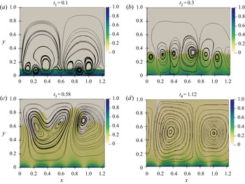
 $T=150< T_c$), which are consistent with the theoretical and numerical investigations of Félici (Reference Félici1971), Lacroix et al. (Reference Lacroix, Atten and Hopfinger1975) and Zhang (Reference Zhang2016). The temporal evolution of flow structures are analysed by choosing four instants from the time series of
 $Ne$ under stochastic boundaries, as shown in the inset of figure 14(a). The flow structures are presented in figure 15. Initially at
 $t_1$, plenty of small rolls start to appear close to the injector (the bottom plate) and they quickly merge with adjacent rolls to form larger roll structures at
 $t_2$. In panel (b), we show that if the flow is able to arrive at a convective state (
 $T=170>T_c$) in the stochastic and deterministic cases, the stochastic case in general requires a much shorter time to reach nonlinear saturation because of the catalyst effect of the stochastic boundary conditions. The green ellipse indicates the increase of
 $Ne$ arising from the stochasticity whereas the grey ellipse represents the intrinsic nonlinear mechanism in the flow that transports the ions. To sum up, the stochastic boundary conditions can bring the flow to the nonlinearly saturated state more easily (requiring a lower
 $T$, as demonstrated in panel (a)) or more quickly (in a shorter time, as demonstrated in panel (b)).
Temporal evolution of electric Nusselt number for electroconvective flows under deterministic (dashed line) and stochastic boundaries (solid line) with  $\sigma =1\,\%$ and
 $l_c=0.5$: (a) time series at
 $T=150$ for both cases (there is no electroconvection in the deterministic case); (b) time series at
 $T=170$ for the stochastic and deterministic cases. All the simulations use
 $\boldsymbol {U}=\phi =Q=0$ as the initial condition.

Temporal development of streamline patterns within the electroconvective flow of  $T=150$ under stochastic boundaries at the four instants shown in figure 14(a). The background contour refers to the distribution of charge density
 $Q$.

Next, we study the effects of perturbation amplitudes  $\sigma$ and correlation lengths
 $l_c$ on linear and nonlinear criteria (i.e.
 $T_c$ and
 $T_f$) represented by a hysteresis loop as shown in figure 16. The red dots are computed by increasing the electric Rayleigh number gradually from the hydrostatic state for indicating the onset of EC and approximating the linear stability criterion
 $T_c$, and the blue dots are obtained by continuously decreasing
 $T$ from the steady state at
 $T=200$ for verifying the nonlinear stability criterion
 $T_f$. At each electric Rayleigh number
 $T$, the group of Gaussian random numbers
 $\xi _k^{(i)}$ has been updated to generate new stochastic boundaries. It is found that the electric Nusselt number
 $Ne$ presents strong fluctuations around the deterministic bifurcation diagram (black lines) under stochastic boundaries. At small perturbation amplitudes, the values of
 $Ne$ distribute very closely to the deterministic bifurcation diagram, while at larger perturbation amplitudes, they fluctuate within a wider range of
 $Ne$ around the deterministic route. Under the same perturbation amplitude, a smaller correlation length (from right to left columns) can induce a wider range of fluctuations. Based on the above definition of stochastic perturbations, a smaller correlation length indicates stronger randomness; thus, it can induce more spatial variations of the electric potential and charge density around the electrodes. Compared with the deterministic bifurcation diagram, with the increase of
 $\sigma$ and decrease of
 $l_c$, the transport efficiency of current can be enhanced (i.e. larger
 $Ne$) with a higher probability. In addition, the EC flow takes place at a smaller
 $T$, as shown in these stochastic bifurcation diagrams, which corroborates the fact that the critical electric Rayleigh number
 $T_c$ of EC flows drops under specific stochastic boundaries. Compared with the result of
 $T_f$ under deterministic boundaries, the stochasticity can also reduce the nonlinear criterion in numerical studies. Furthermore, when intensifying the stochasticity (i.e. by decreasing
 $l_c$ or increasing
 $\sigma$), the distance between
 $T_f$ and
 $T_c$ becomes narrower. Even though we do not know the exact level of the non-uniformality in the ion-exchange membrane (thus the used values of
 $\sigma$ and
 $l_c$ are still arbitrary), this result indicates that the stochasticity in the boundary condition may indeed be important in determining and influencing the linear and nonlinear stability criteria. To close the discussion on this figure, we take panel (h) as the example and mention that there are two clusters of
 $Ne$ values corresponding to the two aforesaid mechanisms inducing the ion transport in the stochastic case. The first is the intrinsic nonlinear mechanism in the flow system, represented by the grey ellipse in figure 16(h). The flow is characterised by a charge-void region as we have discussed above. The second is a stochasticity-promoted mechanism, as shown by the green ellipse, and the value of
 $Ne$ is in general small. This difference between the two cases will be further discussed below.
Stochastic bifurcation diagrams of electroconvective flows around the linear and nonlinear stability criteria with periodic lateral boundaries at  $C=10$,
 $M=10$ and
 $Fe=10^4$. Presented are samples of
 $Ne$ versus
 $T$ corresponding to different choices of
 $\sigma$ and
 $l_c$. The solid line represents the deterministic bifurcation diagram around
 $T_c=162.5$ and
 $T_f=110.4$, and the red and blue dots refer to the
 $Ne$ obtained under stochastic boundary conditions. Red dots are converged
 $Ne$ computed by gradually increasing
 $T$ from the hydrostatic state and blue dots are obtained by gradually decreasing
 $T$ from the steady state of
 $T=200$. The stochastic boundary varies at different
 $T$ for obtaining a more general stochastic bifurcation diagram.

Compared with the deterministic bifurcation diagram, the stochastic boundaries can either enhance or suppress the transport efficiency of electric current. To show their statistical effects on  $Ne$, for some given electric Rayleigh numbers, 2000 computational instances are performed with 2000 profiles of the stochastic boundary conditions (i.e.
 $g_i$ in (2.5) are different) with
 $\sigma =1.0\,\%$ and
 $l_c=0.5$. Based on these samples of
 $Ne$, the probability density function (p.d.f.) is computed, as shown in figure 17. The vertical dashed line represents the corresponding electric Nusselt number in the case of deterministic boundaries. With the stochasticity, it is found that values of
 $Ne$ smaller and higher than the deterministic case are both possible, with a distribution somewhat similar to the Gaussian distribution as the Gaussian random number
 $\xi _k^{(i)}$ has been used. At
 $T=140$ and
 $T=155$ in panels (a) and (b), two peaks exist in the distribution of
 $p(Ne)$. The first peak pertains to the case of small-magnitude convective motions, as shown in the stochastic bifurcation diagram of figure 16(h) (green ellipse), in which
 $Ne$ has a small magnitude, while the second peak corresponds to the case of large-magnitude EC flows (grey ellipse in the same figure). However, as the strength of electric field increases (larger
 $T$), the probability of the emergence for such small-magnitude convective motions gradually decreases. Thus, the stochastic boundary can lead to a higher possibility of enhanced
 $Ne$ compared with that in the deterministic case.
Probability density function  $p(Ne)$ of the electric Nusselt number for electroconvective flows under stochastic boundaries with
 $\sigma =1.0\,\%$ and
 $l_c=0.5$ at six different electric Rayleigh numbers. For comparison, the dashed line represents the value of
 $Ne$ under deterministic boundary conditions. At each
 $T$, 2000 different stochastic boundaries are performed for statistical calculation.

To gain more insights into the influence of stochastic perturbations on EC flows, we perform global linear stability analysis based on the time-stepping Arnoldi method to study the linearised EC flow, as shown in figure 18. It is important to understand that the base flow in this stability analysis is the steady solutions to Maxwell's equations with stochastic boundary conditions (see figure 2b). This base flow is presumably a better representation of the real situation in the experiments compared with the deterministic case because of the stochastic boundary conditions considered. Therefore, the interpretation of the results should be pertaining to this base flow and the  $T_c$ calculated is the critical
 $T$ for the cases in the grey ellipse in figure 16(h) (and alike). The stochasticity-promoted ion transport mechanism is included in the stochastic base flow and thus this linear stability analysis pertains to the intrinsic nonlinear mechanism for the ion transport. The growth rates
 $\omega _r$ of multiple electric Rayleigh numbers have been computed to find
 $T_c$ for nine groups of
 $\sigma$ and
 $l_c$, as shown in figure 18. At very small perturbation amplitude
 $\sigma =0.1\,\%$, the linear stability criterion is very close to that of the deterministic case, as shown in figure 5 with
 $C=10$ and
 $Fe=10^4$. However, with the increase of perturbation amplitude or decrease of correlation length, the stability criterion becomes lower, which means that the stochastic base flow becomes more unstable if we consider stronger stochasticity, which is consistent with the observation in figure 16.
Growth rate of the least stable mode for electroconvective flows under stochastic boundary conditions with different perturbation amplitudes  $\sigma$ and correlation lengths
 $l_c$. Circle, diamond and square symbols refer to the result from the current time-stepping Arnoldi method, the solid lines are the corresponding linear fitted results and the black solid dots are the
 $x$ intercept of the linear fitted line where
 $\omega _r=0$. (a)
 $\sigma =0.1\,\%$:
 $T_c=160.36$ at
 $l_c=0.25$,
 $T_c=162.48$ at
 $l_c=0.5$,
 $T_c=162.55$ at
 $l_c=1.0$; (b)
 $\sigma =2.0\,\%$:
 $T_c=117.46$ at
 $l_c=0.25$,
 $T_c=144.73$ at
 $l_c=0.5$,
 $T_c=157.06$ at
 $l_c=1.0$; (c)
 $\sigma =5.0\,\%$:
 $T_c=90.25$ at
 $l_c=0.25$,
 $T_c=122.16$ at
 $l_c=0.5$,
 $T_c=147.20$ at
 $l_c=1.0$.

4. Conclusions and future works
Prompted by the consideration that the experimental realisation of charge injection and electric potential on electrodes is inevitably inhomogeneous owing to the proneness of the ion-exchange membranes to be non-uniform, contrasted by the homogeneous assumption of the charge injection usually assumed in theoretical and numerical investigations of EC flows, and the fact that transitional EC flows are subcritical, in this work, we explored the possibility of considering stochastic boundary conditions that mimic the aforementioned material inhomogeneity in the modelling of EC flows to attempt to test the hypothesis that the long-standing discrepancy of the linear stability criteria in experimental and theoretical results from such flows may be related to this effect. For a complete description of the flow bifurcations therein as well as a better understanding of the results of the stochastic bifurcations, we first studied the deterministic bifurcation of the EC flow. By doing so, we not only reproduced and verified some of the previous findings (using a more systematic and methodological means), but also found new flow physics and significance. The results are summarised below.
For the deterministic bifurcations with periodic lateral boundaries, we observed the effect of increasing the strength of the electric field, thus nonlinearity, on generating more complex flow structures, manifested as more irregular and chaotic flow structures and signals of  $Ne$, which lead to flow bifurcations. The global bifurcation diagram using the electric Nusselt number
 $Ne$ as a function of electric strength shows clearly how EC flows starting from a hydrostatic state evolve to more complex flows via linear instability, Hopf bifurcation and so on. In this regard, our results are different from the bifurcation diagram of EC flows of Wang & Sheu (Reference Wang and Sheu2016), where the symmetric lateral boundaries were used and the charge diffusion effect was neglected. Such symmetric lateral boundary conditions do not trace the development of the most dangerous mode at stronger electric strength, whereas, in the case of periodic boundary conditions, the current computational domain can accommodate the most dangerous mode even at a larger
 $T$.
Quantitative characterisation of the deterministic bifurcation and chaos in EC flows has also been conducted by probing their Lyapunov exponents, spectrum and dimension. In the case of infinite parallel plates, the largest Lyapunov exponent increases with the strength of the electric field; as does the Lyapunov dimension, which is usually larger than that in natural convection, indicating, to some extent, that the nonlinearity in EC flows is stronger than that in the RBC. In the case of the finite-sized domain with no-slip lateral boundaries, we found for the first time that the chaos in EC flows is extensive, i.e. the Lyapunov dimension scales as the aspect ratio raised to the first power in 2-D flows, which is the same as that in natural convection under the Boussinesq approximation, although EC flows and RBC are featured by different bifurcation mechanisms.
The stochastic bifurcation analysis is applied to EC flows for the first time, with encouraging results. Owing to the subcritical nature of the EC flow, the stochasticity in boundary conditions induces an early onset of the convective motion under different levels of stochasticity as well as intrinsic coherence. Stronger electric fields can better harness the stochasticity to occasionally have a larger  $Ne$. Compared with the deterministic boundary conditions, around the linear criticality, stronger randomness and smaller coherence will lead to a more scattered distribution of
 $Ne$ around the deterministic route. Essentially, the flow can thus be brought to convection at a smaller
 $T_c$ subjected to stochasticity in the boundaries, as shown by our results with both nonlinear evolution and the linear time-stepping Arnoldi method (as a byproduct of our simulations, the finite-amplitude stability criterion
 $T_f$ also drops under such stochastic boundaries). The decreased linear criteria, which are closer to the experimental observations where stochasticity seems inevitable, confirmed our hypothesis made in the beginning. Although the exact degree of stochasticity in experiments is unknown to us (and we are not claiming that the current analysis completely solves the discrepancy), our results indicate that the non-uniformity on the ion-exchange membrane is definitely a factor that needs to be considered when studying the linear criticality in EC flows. Finally, the stochastic model in this work can certainly be improved. More flow physics can be attached to the model if one can come up with a more physical model for the inhomogeneous membranes and if detailed characterisation of the membranes used in EHD experiments is available (to determine the parameter values in the stochastic models).
Therefore, with these results, we suggest as future experimental studies on EC flows that a systematic and comprehensive characterisation of the non-uniformity in ion-exchange membranes needs to be performed. The levels of stochasticity investigated in the current work are admittedly arbitrary, which is not a problem for studying the general effects and trend of stochasticity on the EC flow; however, for a better and more detailed comparison, a coordinated experimental and theoretical study on this problem is necessary. If decreasing the degree of inhomogeneity in the membrane is exceedingly difficult, some stochasticity can be intentionally introduced near the onset of EC flows, which, according to our results above, will reduce the onset  $T_c$ in these flows and lend some support to our conclusions. Furthermore, our results will also be useful for studying in general the effect of other imperfections on the electrodes in the future. We have also focused solely on the SCL regime (which is more easily realised in experiments), so future works can study the weak-injection regime. In the end, we completely miss the more complex bifurcations in three-dimensional EC flows in this work, which will also be interesting to study in the future.
Acknowledgements
We thank all the reviewers for their constructive comments.
Funding
This work was supported by the National University of Singapore (Z.F., Doctoral Research Scholarship); the Start-up grant from the Ministry of Education, Singapore (M.Z., MOE WBS No. R-265-000-619-133); and the Spanish Ministerio de Ciencia, Innovación y Universidades (P.A.V., Research Project No. PGC2018-099217-B-I00).
Declaration of interests
The authors report no conflict of interest.
Appendix A. Ion-exchange membranes and the work by Watson, Schneider & Till (Reference Watson, Schneider and Till1970)
In this appendix, we compile descriptions of the structure in ion-exchange membranes and discuss why the inhomogeneity can be easily formed, as well as how the stochastic perturbations  $g_1(x)$,
 $g_2(x)$ and
 $g_3(x)$ are related to such inhomogeneity.
Owing to the complicated internal structure of ion-exchange membranes (IEM), some ions cannot enter the dielectric liquid smoothly via the pores of the membrane, and such resistance can be attributed to the plugging and adsorption of ions in the pore, as well as the concentration polarisation (CP) of ions in the feed side. When ions or some other particles in the feed solution block the membrane pores, pore plugging can take place. Then the transport number of ions drops around such pores, which can explicitly cause an inhomogeneous injection of ions on the membrane surface. In addition, some anions and cations may be trapped by the membrane pores and they can constitute fixed ion clusters inside the membrane (Moleón & Moya Reference Moleón and Moya2009; Kamcev, Paul & Freeman Reference Kamcev, Paul and Freeman2017). Thus, the internal structure of these membranes becomes heterogeneous owing to the inhomogeneous distribution of fixed ions. By solving the Nernst–Planck and Poisson equations, the symmetric cosinoidal distribution of fixed ions inside the IEM can give rise to increased current efficiency owing to the potential produced by the fixed ions (Selvey & Reiss Reference Selvey and Reiss1985). Under the linear and exponential distributions of fixed charge, the membrane can also present higher permselectivity than the homogeneous membranes, which is mainly determined by the average fixed charge concentration (Sokirko, Manzanares & Pellicer Reference Sokirko, Manzanares and Pellicer1994). Thus, the above inhomogeneous distributions of fixed ions inside the membrane can enhance the transport efficiency of ions through the membrane. Concentration polarisation occurs when ions of opposite polarity accumulate around the membrane surface at the feed side owing to the permselective property of ion exchange membranes (Luis Reference Luis2018). The CP can make conductance non-uniform on the membrane surface and increase the resistance to ion transport through the membrane (Ibanez, Stamatialis & Wessling Reference Ibanez, Stamatialis and Wessling2004). The above resistances to ionic transport originating from pore plugging, pore adsorption, concentration polarisation as well as some other possible sources can affect the permselectivity of ions (Takagi, Vaselbehagh & Matsuyama Reference Takagi, Vaselbehagh and Matsuyama2014), thus the injection of ions through the IEM is not uniform, and the gain/loss of ions can be modelled by the stochastic perturbation  $g_1(x)$. Furthermore, the resistance to ionic transport can induce extra potential differences according to Ohm's law (Galama, Hoog & Yntema Reference Galama, Hoog and Yntema2016), which indicates that the potential distribution on the membrane surface can also be non-uniform. Thus, the random perturbations
 $g_2(x)$ and
 $g_3(x)$ are used to incorporate the extra potential differences into the numerical study of EC flows. More refined profiles of
 $g_1(x)$,
 $g_2(x)$ and
 $g_3(x)$ can be certainly obtained when the characterisation of the membranes used in EHD experiments is available, as we have discussed in the conclusion.
In fact, Schneider & Watson (Reference Schneider and Watson1970) have already pointed out that the non-uniformness on the metal electrodes has a detrimental effect to realising homogeneous injection. Thus in their experiment, the ion exchange membrane and metal electrode (i.e. the composite metal–membrane electrode Atten & Gosse Reference Atten and Gosse1969; Lacroix et al. Reference Lacroix, Atten and Hopfinger1975) were replaced by an electron beam that served as a virtual cathode, which injected electrons into the free surface of the dielectric liquid. The use of electron beams in their experiment eliminated the potential effects of ion-exchange membranes on EC flows. Interestingly, they found that the critical voltage indicating onset of convection obtained in their experiments agreed well with their corresponding theoretical studies (Schneider & Watson Reference Schneider and Watson1970) (both yielding a linear stability criterion  $T_c\approx 99$. In their notation,
 $R$ was used). To some extent, the consistency of their experimental and theoretical results adds to the culpability of the above composite electrode on generating the discrepancy of the linear stability criterion in the EC flows using ion-exchange membranes.
Appendix B. Deterministic bifurcation diagram with symmetric lateral boundaries
The deterministic bifurcation diagram under symmetric lateral boundaries (B1) is shown in figure 19. The spatial domain is  $[0,0.614]$ at the
 $x$ axis (i.e.
 $L=0.614$),
 $[0,1]$ at the
 $y$ axis, and other parameters are
 $C=10$,
 $M=10$ and
 $Fe=10^4$. When the electric Rayleigh number is smaller than the linear stability criterion
 $T_c$ (
 ${=}162.5$ as verified in the previous section), the fluid stays in the hydrostatic state. Once
 $T>T_c$, the transition from conduction to convection takes place, and a one-roll convection pattern is generated, as shown in figure 20(a). In numerical simulations, this convection pattern can show two different rotational motions based on the initial conditions, one in the clockwise roll and the other in the anticlockwise roll, which are intrinsically the same owing to the symmetric conditions on the lateral wall. With the successive increase of
 $T$, the Hopf bifurcation within the range of the one-roll pattern occurs at approximately
 $T_{c1}=295$. Then this one-roll flow structure becomes unstable, and divides into two rolls when the electric Rayleigh number increases to approximately
 $T_{c2}=311$. This steady two-roll structure, as shown in figure 20(b), can be retained for a wide range of
 $T$. Later, its motion becomes periodically unsteady after approximately
 $T_{c3}=660$, where the Hopf bifurcation takes place.
 $$\begin{gather} y=0: \ \boldsymbol{U}=0, \, Q=1, \, \phi=1; \end{gather}$$
 $$\begin{gather}y=1: \ \boldsymbol{U}=0, \, \partial Q/\partial y=0, \, \phi=0; \end{gather}$$
 $$\begin{gather}x=0 \ \& \ x=L: \ U=0, \, \partial V/\partial x=0, \, \partial Q/\partial x=0, \, \partial \phi/\partial x=0. \end{gather}$$
Deterministic bifurcation diagram for electroconvective flows with symmetric lateral boundaries. The Hopf bifurcation for the one-roll pattern takes place at approximately  $T_{c1}=295$, and the one roll is split into two rolls at approximately
 $T_{c2}=311$. The Hopf bifurcation for two-roll pattern ensues at approximately
 $T_{c3}=660$.

Contour of charge density and streamline patterns of electroconvective flows with symmetric lateral boundaries. To clearly show at least one complete charge-void region, the flow domain is unfolded with respect to  $x=0$ owing to the symmetric boundary in the lateral direction: (a)
 $T=190$, one-roll flow structure emerges within
 $[0,0.614]$ of the
 $x$ axis; (b)
 $T=340$, two-roll flow structure takes place within
 $[0,0.614]$ of the
 $x$ axis.

With the further increase of the electric Rayleigh number, more extreme values of the electric Nusselt number appear in the bifurcation diagram for a specific  $T$, and the EC flow is believed to enter the chaotic state. From the bifurcation diagram in figure 19, the chaos seems to take place in the range between
 $T=900$ and
 $T=950$. To distinguish such chaos from the numerically obtained signals of
 $Ne$, their power distributions across frequency are presented by calculating the power spectral density as the analysis of experimental signals in the works of Atten et al. (Reference Atten, Lacroix and Malraison1980), Malraison & Atten (Reference Malraison and Atten1982), and our results are shown in figure 21. At
 $T=670$ and
 $T=800$, a discrete sharp central peak and its harmonics can be clearly discerned. With the increase of electric Rayleigh number, the number of peaks increases, and the power spectrum starts to become broadband, which indicates the appearance of chaos. At
 $T=900$ and
 $T=920$, their power spectra are featured by broadband wiggles and oscillations, which confirms that the chaos of the current EC flow increases in the range of
 $[900,920]$. In addition, the largest Lyapunov exponent
 $\lambda _1$ is also computed to evidence the onset of chaos in the above EC flows, as shown in table 4. It is found that
 $\lambda _1$ is positive at
 $T=920$ but negative at
 $T=900$, which provides a more accurate and systematic prediction of the appearance of chaos within the range of
 $T\in [900,920]$.
Power spectral density for the time series of electric Nusselt number at different electric Rayleigh numbers with symmetric lateral boundaries. The spectrum starts to become broadband around  $T=920$.

Largest Lyapunov exponents  $\lambda _1$ and Lyapunov dimensions
 $D_{\lambda }$ of electroconvective flows at different electric Rayleigh numbers
 $T$ with symmetric lateral boundaries.

This sequence of bifurcations for the EC flow under symmetric lateral boundaries has shown some similarity to that reported by Wang & Sheu (Reference Wang and Sheu2016). However, the difference is that the charge diffusion effect was not considered in their work. Under the same parameters, their bifurcation criteria are, using our notations,  $T_c=164$,
 $T_{c1}=213$,
 $T_{c2}=281$ and
 $T_{c3}=419$, which are different from our values. When the charge diffusion effect increases, the linear stability criterion
 $T_c$ decreases, thus our estimated
 $T_c$ is smaller than theirs. In addition, the charge diffusion can help stabilise the finite-amplitude oscillations in the flow (Zhang Reference Zhang2016), which explains that higher electric Rayleigh numbers must be required for Hopf bifurcation and roll structure transition with charge diffusion considered; thus, our
 $T_{c1},T_{c2}$ and
 $T_{c3}$ values are larger than theirs (Wang & Sheu Reference Wang and Sheu2016).
As one can see, the bifurcation results using the symmetric boundary conditions are different from those using the periodic boundary conditions. In the latter case, the EC flow bifurcates and becomes chaotic at a smaller value of  $T$. This is consistent with our discussion in the main text that using the periodic boundary conditions can follow the most dangerous bifurcation route because the wavelength of the most dangerous mode decreases as we increase
 $T$ (see Appendix C), whereas using the symmetric boundary conditions, one is confined to tracing the bifurcation route of the waves for which the computational length
 $L$ is an integer multiple of the half-wavelength, which is not necessarily the most dangerous mode when one increases
 $T$.
Appendix C. Effects of electric Rayleigh number on wavelengths of the least stable mode
To present the inappropriateness of using symmetric lateral boundaries at higher electric Rayleigh numbers, the effect of  $T$ on the wavelength of the least stable mode of EC flows is studied in this appendix by evolving nonlinear EHD equations (2.1) with periodic lateral boundaries. Initially, an impulse disturbance, which serves as the wave packet with a broad spectrum structure, is added into the hydrostatic field of the EC flow, as shown in figure 22. The profiles of this impulse follow those of Delbende & Chomaz (Reference Delbende and Chomaz1998) with
 $\sigma _x=0.3$ along the
 $x$ axis and
 $\sigma _y=0.2$ along the
 $y$ axis, which read:
 $$\begin{gather} U(x,y,t=0) ={-}A(y-y_0) \exp \left[ -\left( \frac{(x-x_0)^2}{2\sigma_x^2} + \frac{(y-y_0)^2}{2\sigma_y^2} \right) \right] , \end{gather}$$
 $$\begin{gather}V(x,y,t=0) ={-}A(x-x_0) \frac{\sigma_y^2}{\sigma_x^2} \exp \left[ -\left( \frac{(x-x_0)^2}{2\sigma_x^2} + \frac{(y-y_0)^2}{2\sigma_y^2} \right) \right], \end{gather}$$
where  $x_0=60$,
 $y_0=0.5$ refer to the central location of the impulse, and the perturbation amplitude is set to
 $A=10^{-5}$. The envelope of this initial disturbance is Gaussian, and it satisfies the requirement of the continuity equation (2.1d).
Distribution of the impulse disturbance added into the hydrostatic field of electroconvective flows: (a) streamwise velocity  $U(x,y,t=0)$; (b) normal velocity
 $V(x,y,t=0)$. Their initial perturbation amplitude is very small. Only part of the flow field is presented here for a clear visualisation as the impulse is distributed around the central location
 $x_0=0.5$ and
 $y_0=60$.

By considering the temporal evolution of the EC energy spectrum (i.e. (2.11)) for this wave packet in spectral space (i.e. performing a fast Fourier transform on  $\mathcal {E}$ along the streamwise direction), the leading growth rate
 $\omega _r(\alpha )$ can be calculated for each streamwise wavenumber
 $\alpha$ (Delbende & Chomaz Reference Delbende and Chomaz1998). Note that the computational domain is long enough and the periodic boundary conditions are applied on the lateral walls. In the current case, the spatial range is set to
 $[0,120]$ at the
 $x$ axis and
 $[0,1]$ at the
 $y$ axis, the parameters are
 $C=10$,
 $M=10$ and
 $Fe=10^4$.
At  $T=190$, the variation of the temporal growth rate
 $\omega _r$ with streamwise wavenumber
 $\alpha$ is shown in figure 23(a). The current result agrees very well with those from the local linear stability analysis in the work of Zhang et al. (Reference Zhang, Martinelli, Wu, Schmid and Quadrio2015). Note that we use a very small amplitude of the impulse disturbance, so that the nonlinearity is not strongly triggered in the early evolving stage. The wavenumber corresponding to the leading growth rate is
 $\alpha _l=5.1313$, and the wavelength is
 $L=2{\rm \pi} / \alpha _l=1.2245$, which is very close to the spatial length applied in the above bifurcation analysis. As the electric Rayleigh number
 $T$ increases, the wavenumber of the least stable mode is found to increase, as presented in figure 23(b), which indicates that the wavelength of the least stable mode decreases at higher
 $T$. Thus, in the current work, the use of periodic lateral boundaries with
 $L=1.228$ can always allow the free development of the least stable mode (in the linear stage) at higher electric Rayleigh numbers, while the symmetric lateral boundaries restrict the linear EC flow with some quantised wavelengths.
Linear response of the impulse disturbance: (a) variation of temporal growth rate  $\omega _r$ with the streamwise wavenumber
 $\alpha$ at
 $T=190$. The circles refer to the current result, and the solid line is the result from the local linear stability analysis (Zhang et al. Reference Zhang, Martinelli, Wu, Schmid and Quadrio2015); (b) relation between the wavenumber of the least stable mode
 $\alpha _l$ and the electric Rayleigh number
 $T$. Note that the step-shape result for small values of
 $\alpha _l$ is related to the smallest increment of wavenumber. A longer streamwise length
 $L$ can mitigate this problem. However, the comparison of results between DNS (circles) and the linear stability analysis (the solid line) clearly indicates the trend that the wavenumber of the least stable mode
 $\alpha _l$ increases with
 $T$.