1. Introduction
Multiphase flows in complex geometries have many applications in the physical and biological sciences. To numerically simulate such physical phenomena involves solving interfacial problems with complex geometries and moving contact lines that separate fluid components at solid boundaries. In addition, special treatment of the contact line is needed to regularize the stress singularity. These are highly challenging problems for numerical simulation. Using standard discretization methods to solve these problems requires a triangulation of the complicated domain and thus rules out coarse-scale discretizations and with it efficient multilevel solutions. Many numerical methods have been developed for solving multiphase flows in complex geometries. Examples are fictitious domain methods (Glowinski et al. Reference Glowinski, Pan, Hesla, Joseph and Périaux2001; Zhang et al. Reference Zhang, Walayat, Chang and Liu2018), extended finite element methods (Fries & Belytschko Reference Fries and Belytschko2010), immersed boundary methods (Schneider Reference Schneider2015; Stein, Guy & Thomases Reference Stein, Guy and Thomases2017), immersed interface methods (Li Reference Li2003; Chen, Li & Lin Reference Chen, Li and Lin2007; Gong et al. Reference Gong, Zhao, Yang and Wang2018; O'Brien & Bussmann Reference O'Brien and Bussmann2018) and the volume penalty method (Shirokoff & Nave Reference Shirokoff and Nave2014; De Stefano, Nejadmalayeri & Vasilyev Reference De Stefano, Nejadmalayeri and Vasilyev2016), where the complex geometry is embedded in a larger, regular domain with a test function being used to enforce the boundary conditions at solid–fluid interfaces. Other methods include boundary integral methods (Biros, Ying & Zorin Reference Biros, Ying and Zorin2004; Mittal et al. Reference Mittal, Dong, Bozkurttas, Najjar, Vargas and von Loebbecke2008), which explicitly incorporate the boundary conditions in the reformulated equations, front-tracking methods (Tryggvason et al. Reference Tryggvason, Bunner, Esmaeeli, Juric, Al-Rawahi, Tauber, Han, Nas and Jan2001; Zolfaghari, Izbassarov & Muradoglu Reference Zolfaghari, Izbassarov and Muradoglu2017) and arbitrary Eulerian–Lagrangian methods (Hu, Patankar & Zhu Reference Hu, Patankar and Zhu2001; Gilmanov & Sotiropoulos Reference Gilmanov and Sotiropoulos2005; Anjos et al. Reference Anjos, Mangiavacchi, Borhani and Thome2013) that utilize a separate Lagrangian mesh to track the complex boundary and either smear the boundary conditions across several mesh points or explicitly enforce the boundary conditions on the Lagrangian mesh that cuts across the Eulerian mesh using body forces or modified discretizations. Methods along these lines include level-set, ghost-fluid, volume of fluid/level-set and cut-cell methods (Kirkpatrick, Armfield & Kent Reference Kirkpatrick, Armfield and Kent2003; Gao et al. Reference Gao, Ingram, Causon and Mingham2007; Herrmann Reference Herrmann2008; de Zélicourt et al. Reference de Zélicourt, Ge, Wang, Sotiropoulos, Gilmanov and Yoganathan2009; Zhang & Ni Reference Zhang and Ni2014; Gutiérrez et al. Reference Gutiérrez, Favre, Balcázar, Amani and Rigola2018; Cao et al. Reference Cao, Sun, Wei, Yu and Li2019). However, most of these methods require modifications of standard finite element or finite difference software packages.
The diffuse domain (DD) method was proposed in Li et al. (Reference Li, Lowengrub, Rätz and Voigt2009) to solve partial differential equations in stationary/moving complex geometries with Dirichlet, Neumann or Robin boundary conditions. In this method, the complex geometry is extended to a larger, regular domain and a phase-field function is used to smoothly approximate the characteristic function of the original domain. The original partial differential equation is then reformulated on the larger domain with additional source terms that approximate the boundary conditions. It has been shown that the reformulated partial differential equation asymptotically converges to the original system as the width of the diffuse interface layer tends to zero (Li et al. Reference Li, Lowengrub, Rätz and Voigt2009; Yu, Chen & Thornton Reference Yu, Chen and Thornton2012; Lervag & Lowengrub Reference Lervag and Lowengrub2015; Chadwick et al. Reference Chadwick, Stewart, Enrique, Du and Thornton2018; Poulsen & Voorhees Reference Poulsen and Voorhees2018; Yu, Guo & Lowengrub Reference Yu, Guo and Lowengrub2020). The advantages of such a method are that no modifications of standard software packages are required and the stationary/moving complex boundary can be imposed easily and smoothly.
The DD method has recently been coupled with a standard two-phase diffuse interface model to study two-phase fluid flows in complex geometries (Aland, Lowengrub & Voigt Reference Aland, Lowengrub and Voigt2010), where the fluid model is restricted to the case that the densities and viscosities of the two fluids are exactly the same. Phase-field, or diffuse interface, models have now emerged as a powerful method to simulate many types of multiphase flows (Guo, Lin & Lowengrub Reference Guo, Lin and Lowengrub2014a; Guo, Lin & Wang Reference Guo, Lin and Wang2014b; Guo & Lin Reference Guo and Lin2015; Jiang et al. Reference Jiang, Lin, Guo and Dong2015; Zhang & Wang Reference Zhang and Wang2016; Guo et al. Reference Guo, Lin, Lowengrub and Wise2017). The basic idea is to introduce a phase variable (order parameter) that varies continuously over thin interfacial layers and is mostly uniform in the bulk phases. In this way the phase variable can characterize different fluid component regions. Sharp interfaces are replaced by thin transition regions with non-zero thickness. One set of governing equations for the whole computational domain can be derived using variational techniques with respect to a free energy. The order parameter fields satisfy an advection–diffusion equation (usually the advective Cahn–Hilliard equations) and are coupled to Navier–Stokes-type equations through extra reactive stresses that mimic surface tension.
The classical phase-field model, Model H (Hohenberg Reference Hohenberg1977), was initially developed for simulating a binary incompressible fluid with density-matched components, and was later generalized for simulating binary incompressible fluids with variable density components (Boyer Reference Boyer2002; Ding, Spelt & Shu Reference Ding, Spelt and Shu2007; Abels, Garcke & Grun Reference Abels, Garcke and Grun2012; Dong & Shen Reference Dong and Shen2012; Aki et al. Reference Aki, Dreyer, Giesselmann and Kraus2014; Gong, Zhao & Wang Reference Gong, Zhao and Wang2017; Gong et al. Reference Gong, Zhao, Yang and Wang2018; Shokrpour Roudbari et al. Reference Shokrpour Roudbari, Şimşek, van Brummelen and van der Zee2018). Some of these models, however, do not satisfy Galilean invariance, local mass conservation or are not thermodynamically consistent. A challenge is maintaining local mass conservation, thermodynamic consistency and Galilean invariance. In Lowengrub & Truskinovsky (Reference Lowengrub and Truskinovsky1998), Model H was extended to a thermodynamically consistent model for variable density flows using the mass concentration as the phase variable and the mass-averaged velocity as the velocity field. Moreover, the fluids mix at the interfacial region which generates changes in the density even if the fluid components are incompressible individually. Such a system was called quasi-incompressible and leads to a (generally) non-solenoidal velocity field ( $\boldsymbol {\nabla }\boldsymbol {\cdot } \boldsymbol {v}\ne 0$) and an extra pressure term appears in the Cahn–Hilliard equation compared to Model H. More recently, two other quasi-incompressible phase-field models (Gong et al. Reference Gong, Zhao and Wang2017; Shokrpour Roudbari et al. Reference Shokrpour Roudbari, Şimşek, van Brummelen and van der Zee2018) were developed to study binary fluids with variable densities, where the volume fraction was employed as the phase variable and a different free energy was used for the model derivations.
In this paper, we couple the DD method and a two-phase diffuse interface model to simulate binary flow in complex geometries. In particular, we first develop a thermodynamically consistent diffuse interface model, which we refer to as the quasi-incompressible Navier–Stokes Cahn–Hilliard model (q-NSCH), that allows for large density and viscosity differences between the two fluids. The model also employs the volume fraction as the phase variable. Compared to the models in Gong et al. (Reference Gong, Zhao and Wang2017) and Shokrpour Roudbari et al. (Reference Shokrpour Roudbari, Şimşek, van Brummelen and van der Zee2018), we use a different free energy and a different derivation framework that leads to a simple formulation of the system equations. We then combine the DD method with the q-NSCH system, namely the q-NSCH-DD model, to simulate two-phase flows in complex geometries. We perform a matched asymptotic analysis for the q-NSCH-DD model to show that it converges to the original q-NSCH model as the thickness of the DD interface shrinks to zero ( $\epsilon \rightarrow 0$) with first-order accuracy, e.g.
 $O(\epsilon )$. We present several numerical tests that illustrate the flexibility and accuracy of the approach.
The outline of the paper is as follows. In § 2, we present our q-NSCH model and, in § 3, its DD reformulation (the q-NSCH-DD system). Appendix A shows the asymptotic analysis of the q-NSCH-DD model. The numerical method and its implementation are described in appendix B. In § 4, we show several numerical simulations and results. Finally in § 5, we share some parting thoughts about the work presented here.
2. Derivation of the q-NSCH model
Here we follow the thermodynamic framework in Guo & Lin (Reference Guo and Lin2015) and derive a new diffuse interface model for two-phase flows with variable density and viscosity. The model equations are derived through a variational procedure that guarantees thermodynamic consistency.
2.1. Phase variable and variable density
Suppose in a control volume  $V$ we have two fluids (labelled by
 $i= 1,2$) that fill volumes
 $V_{i}$ separately. The volume fraction for the
 $i$th fluid can be given by
 $c_{i}= {V_{i}}/{V}$. Further we assume that the two fluids can mix within an interfacial region separating the two fluids and the volume occupied by a given amount of mass of the single fluid does not change after mixing. Therefore
 $c_1+c_2=1$ within the control volume
 $V$. Given the total mass and volume for the mixture,
 $M=M_{1}+M_{2}$ and
 $V=V_{1}+V_{2}$, we introduce the actual local mass density
 $\rho _{i}$ for each fluid, and the local volume-averaged mass density
 $\tilde {\rho }_{i}$ taken over a sufficient small volume
 $V$:
 \begin{equation} \rho_{i}=\frac{M_{i}}{V_{i}},\quad \tilde{\rho}_{i}=\frac{M_{i}}{V}=\frac{M_{i}}{V_{i}}\frac{V_{i}}{V}=\rho_{i}c_{i}, \end{equation}
where  $\rho _i$ is a positive constant. We then define the volume-averaged density of the mixture as
 \begin{equation} \rho=\tilde{\rho}_{1}+\tilde{\rho}_{2}=\rho_{1}c_{1}+\rho_{2}c_{2}. \end{equation}
Since  $c_{1}+c_{2}=1$, we assume that the phase variable with respect to volume fraction is given by
 $c=c_{1}=1-c_{2}$. The corresponding variable density for the mixture can be rewritten as
 \begin{equation} \rho=(\rho_{1}-\rho_{2})c+\rho_{2}. \end{equation}
Suppose that the two fluids move with different velocities  $\boldsymbol {u}_i(\boldsymbol {x},t)$, then mass conservation for the mixture is given by
 \begin{equation} \partial_{t}(\tilde{\rho}_{1}+\tilde{\rho}_{2})+\boldsymbol{\nabla}\boldsymbol{\cdot} (\tilde{\rho}_{1}\boldsymbol{u}_{1}+\tilde{\rho}_{2}\boldsymbol{u}_{2})=0. \end{equation}
The mass-averaged velocity  $\boldsymbol {u} := {(\tilde {\rho }_{1}\boldsymbol {u}_{1}+\tilde {\rho }_{2}\boldsymbol {u}_{2})}/{\rho }$ and
 $\rho$, defined in (2.2), satisfy the mass conservation equation:
 \begin{equation} \partial_{t}\rho+\boldsymbol{\nabla}\boldsymbol{\cdot}(\rho\boldsymbol{u})=0. \end{equation}
2.2. Balance laws
We next consider the balance laws for the two-fluid mixture. Suppose the two-phase fluid is combined in a domain  $\varOmega$. We then take an arbitrary control volume
 $V(t)\subset \varOmega$ that moves with the mixture. Within the control volume, we define the following quantities for the two-phase fluid:
 \begin{gather} M=\int_{V(t)}\rho\,{\mathrm d}V, \end{gather}
 \begin{gather}{\boldsymbol{P}}=\int_{V(t)}\rho\boldsymbol{u}\,{\mathrm d}V, \end{gather}
 \begin{gather}E=\int_{V(t)}\left( \frac{1}{2}\rho |\boldsymbol{u}|^2+\tilde{\sigma} F(c)+ \frac{\tilde{\sigma}\epsilon_c |\boldsymbol{\nabla} c|^2}{2}-\rho g \boldsymbol{z}\right){\mathrm d}V, \end{gather}
 \begin{gather}C=\int_{V(t)}c\,{\mathrm d}V, \end{gather}
where  $M$,
 $\boldsymbol {P}$,
 $E$ and
 $C$ are the total mass, momentum, free energy and constituent volume of fluid 1 within the control volume
 $V(t)$. Further,
 $\rho (c)$ is the variable density of the mixture,
 $\boldsymbol {u}$ is the mass-averaged velocity of the mixture,
 $|\boldsymbol {u}|^2/2$ is the kinetic energy per unit mass,
 $g$ is the gravitational constant,
 $\boldsymbol {z}$ is the vector in the vertical direction,
 $\tilde {\sigma } F(c)+{\tilde {\sigma }\epsilon _c |\boldsymbol {\nabla } c|^2}/{2}$ is the Cahn–Hilliard-type interfacial free energy,
 $F(c)=c^2(c-1)^2/4\epsilon _c$ is double-well potential,
 $\epsilon _c$ is a small parameter that characterizes the thickness of the diffuse interface separating the fluid components and
 $\tilde {\sigma }$ is the surface tension that is related to the physical surface tension
 $\sigma$ through
 $\sigma =6\sqrt {2}\tilde {\sigma }$. The general forms of the physical balance laws associated with
 $M$,
 $\boldsymbol {P}$,
 $E$ and
 $C$ can be given as follows:
 \begin{gather} \frac{{\mathrm{d}} M}{\mathrm{d}t}=0, \end{gather}
 \begin{gather}\frac{{\mathrm{d}} \boldsymbol{P}} {\mathrm{d} t}= \int_{\partial V(t)} {\boldsymbol{\mathsf{m}}}\boldsymbol{\cdot} \boldsymbol{n}\, \mathrm{d}A -\int_{V(t)} \rho g \boldsymbol{z}\,{\mathrm{d}} V, \end{gather}
 \begin{gather}\frac{{\mathrm{d}} E}{{\mathrm{d}}t}= -\int_{\partial V(t)} {\boldsymbol{\mathsf{q}}}_{E}\boldsymbol{\cdot} \boldsymbol{n}\, {\mathrm{d}}A+\int_{V(t)} D\,{\mathrm{d}}V\quad (D\leqslant 0), \end{gather}
 \begin{gather}\frac{{\mathrm{d}} C}{{\mathrm{d}}t}= -\int_{\partial V(t)} {\boldsymbol{\mathsf{q}}}_{C}\boldsymbol{\cdot} \boldsymbol{n}\,{\mathrm{d}}A, \end{gather}
where  ${\boldsymbol{\mathsf{m}}}$ is a tensor,
 ${\boldsymbol{\mathsf{q}}}_{E}$ and
 ${\boldsymbol{\mathsf{q}}}_{C}$ are fluxes and
 $D$ is the dissipation function, which will be specified later. The mass balance (2.10) ensures (2.5) is satisfied. The momentum balance (2.11) leads to
 \begin{equation} \rho \frac{{\mathrm{D}}\boldsymbol{u} }{{\mathrm{D}}t}={\boldsymbol{\nabla}} \boldsymbol{\cdot} {\boldsymbol{\mathsf{m}}}-\rho g \boldsymbol{z},\end{equation}
where  ${{\mathrm {D}}}/{{\mathrm {D}}t}=\partial _{t}+\boldsymbol {u} \boldsymbol {\cdot } \boldsymbol {\nabla }$. The constituent volume balance equation (2.13) gives that
 \begin{equation} \frac{{\mathrm D}c}{{\mathrm D} t}+c(\boldsymbol{\nabla}\boldsymbol{\cdot} \boldsymbol{u} )=-{\boldsymbol{\nabla}}\boldsymbol{\cdot} {\boldsymbol{\mathsf{q}}}_{C}. \end{equation}
Further, by using the definition of  $\rho$ in (2.3) and the mass conservation (2.5), we obtain
 \begin{equation} \boldsymbol{\nabla}\boldsymbol{\cdot}\boldsymbol{u}=- \frac{1}{\rho}\frac{{\mathrm D}\rho}{{\mathrm D}t}=- \frac{{\mathrm d}\rho}{\rho\,{\mathrm d}c}\frac{{\mathrm D}c}{{\mathrm D}t}= \frac{\rho_{2}-\rho_{1}}{\rho}\frac{{\mathrm D}c}{{\mathrm D}t}. \end{equation}
Substituting  ${{\mathrm D}c}/{{\mathrm D}t}$ in (2.15), we obtain the quasi-incompressibility in the interfacial region for the two-phase flows:
 \begin{equation} \boldsymbol{\nabla}\boldsymbol{\cdot} \boldsymbol{u}=-\alpha\boldsymbol{\nabla}\boldsymbol{\cdot} {\boldsymbol{\mathsf{q}}}_{C},\end{equation}
where  $\alpha =(\rho _{2}-\rho _{1})/\rho _{2}$.
We now consider the energy balance (2.12). We first take the time derivative of the free energy (2.8) to obtain
 \begin{align} \frac{{\mathrm d} E}{{\mathrm d}t}&= \int_{V(t)} \left\{\rho \boldsymbol{u}\boldsymbol{\cdot} \frac{{\mathrm D}\boldsymbol{u}}{{\mathrm D}t}+\left(\tilde{\sigma} F'(c)- \tilde{\sigma}\epsilon_c {\rm \Delta} c\right)\frac{{\mathrm D}c}{{\mathrm D}t}+{\boldsymbol{\nabla}} \boldsymbol{\cdot} \left(\tilde{\sigma}\epsilon_c\frac{{\mathrm D}c}{{\mathrm D}t}{ \boldsymbol{\nabla}}c\right)\right.\nonumber\\ &\quad \left.-\tilde{\sigma}\epsilon_c \left({\boldsymbol{\nabla}} c \otimes {\boldsymbol\nabla} c\right): {\boldsymbol\nabla} \boldsymbol{u}+ \left(\tilde{\sigma} F(c)+\frac{\tilde{\sigma}\epsilon_c |\boldsymbol{\nabla} c|^2}{2}\right)\left( \boldsymbol{\nabla}\boldsymbol{\cdot}\boldsymbol{u} \right)-\rho g \boldsymbol{u}\boldsymbol{\cdot} \boldsymbol{z}\right\}{\mathrm d}V, \end{align}
where we have used the following identities:
 \begin{align} \frac{\mathrm D}{{\mathrm D}t}\left(F\left(c\right)+\frac{\epsilon_c|{\boldsymbol\nabla} c|^2}{2}\right)&=F'\left(c\right)\frac{{\mathrm D}c}{{\mathrm D}t}-{\rm \Delta} c\frac{{\mathrm D}c}{{\mathrm D}t}+{\boldsymbol\nabla}\boldsymbol{\cdot}\left({\boldsymbol\nabla} c\frac{{\mathrm D}c}{{\mathrm D}t}\right) \nonumber\\ &\quad -\left({\boldsymbol\nabla} c\otimes {\boldsymbol\nabla} c\right): {\boldsymbol\nabla} \boldsymbol{u}, \end{align}
 \begin{equation} {\boldsymbol\nabla} c \boldsymbol{\cdot} \frac{\mathrm D}{{\mathrm D}t}{\boldsymbol\nabla} c= {\boldsymbol\nabla} c \boldsymbol{\cdot}\left({\boldsymbol\nabla} c_{t} + \boldsymbol{u}\boldsymbol{\cdot{}\boldsymbol\nabla}\left({\boldsymbol\nabla} c\right)\right), \end{equation}
 \begin{equation}{\boldsymbol\nabla} c \boldsymbol{\cdot} {\boldsymbol\nabla} c_{t} = {\boldsymbol\nabla}\boldsymbol{\cdot} \left({\boldsymbol\nabla} c c_{t} \right)-{\rm \Delta} c c_{t}, \end{equation}
 \begin{align} {\boldsymbol\nabla} c \boldsymbol{\cdot} \left( \boldsymbol{u}\boldsymbol{\cdot}{\boldsymbol\nabla} \left({\boldsymbol\nabla} c\right)\right)&={\boldsymbol\nabla}\boldsymbol{\cdot} \left({\boldsymbol\nabla} c \left( \boldsymbol{u}\boldsymbol{\cdot}{\boldsymbol\nabla} c\right)\right)- {\rm \Delta} c \left(\boldsymbol{u}\boldsymbol{\cdot}{\boldsymbol\nabla} c\right)\nonumber\\ &\quad -\left({\boldsymbol\nabla} c \otimes {\boldsymbol\nabla} c\right): {\boldsymbol\nabla}\boldsymbol{u}. \end{align}
Substituting  $\rho ({{\mathrm D}\boldsymbol {u}}/{{\mathrm D}t})$ and
 ${{\mathrm D}c}/{{\mathrm D}t}$ in (2.14) and (2.15), respectively, and applying the divergence theorem, we obtain
 \begin{align} \frac{{\mathrm D}E}{{\mathrm D}t}&= \int_{V(t)} \left\{{\boldsymbol\nabla} \boldsymbol{\cdot}\left( {\boldsymbol{\mathsf{m}}} \cdot \boldsymbol{u} +\tilde{\sigma}\epsilon_c\frac{{\mathrm D} c}{{\mathrm D}t}{\boldsymbol\nabla} c\right)- \left({\boldsymbol{\mathsf{m}}}_0 +\tilde{\sigma}\epsilon_c ({\boldsymbol\nabla} c \otimes {\boldsymbol\nabla} c)+{\tau}\right): {\boldsymbol \nabla}\boldsymbol{u}\right. \nonumber\\ &\quad - \left(-\tilde{\sigma} F(c)-\frac{\tilde{\sigma}\epsilon_c | \boldsymbol{\nabla} c|^2}{2}+\left(\tilde{\sigma} F'(c)-\tilde{\sigma}\epsilon_c {\rm \Delta} c\right)c\right) {\boldsymbol\nabla}\boldsymbol{\cdot} \boldsymbol{u}\nonumber\\ &\quad \left.\vphantom{\left( {\boldsymbol{\mathsf{m}}} \cdot \boldsymbol{u} +\tilde{\sigma}\epsilon_c\frac{{\mathrm D} c}{{\mathrm D}t}{\boldsymbol\nabla} c\right)}- {\boldsymbol\nabla} \boldsymbol{\cdot}\left( \tilde{\sigma}\left(F'(c)- \epsilon_c{\rm \Delta} c\right) {\boldsymbol{\mathsf{q}}}_{C}\right)+{\boldsymbol{\mathsf{q}}}_{C} \boldsymbol{\cdot} {\boldsymbol\nabla} \left(\tilde{\sigma}\left(F'(c)-\epsilon_c{\rm \Delta} c\right) \right)\right\}{\mathrm d}V\nonumber\\ &=\int_{V(t)} \left\{{\boldsymbol\nabla} \boldsymbol{\cdot}\left( {\boldsymbol{\mathsf{m}}} \boldsymbol{\cdot} \boldsymbol{u} +\tilde{\sigma}\epsilon_c \frac{{\mathrm D} c}{{\mathrm D}t}{\boldsymbol\nabla} c\right)- \left({\boldsymbol{\mathsf{m}}}_0 +\tilde{\sigma}\epsilon_c ({\boldsymbol\nabla} c \otimes {\boldsymbol\nabla} c) \right): {\boldsymbol D}\boldsymbol{u}-{\tau}:{\boldsymbol\nabla} \boldsymbol{u} \right. \nonumber\\ &\quad - \left({\boldsymbol{\mathsf{m}}}_0 +\tilde{\sigma} \epsilon_c ({\boldsymbol\nabla} c \otimes {\boldsymbol\nabla} c) -\tilde{\sigma} F(c) {\boldsymbol{\mathsf{I}}}-\frac{\tilde{\sigma}\epsilon_c | \boldsymbol{\nabla} c|^2}{2}{{\boldsymbol{\mathsf{I}}}}\!+\! \left(\tilde{\sigma} F'(c)-\tilde{\sigma}\epsilon_c{\rm \Delta} c\right)c {\boldsymbol{\mathsf{I}}}\right): \frac{{\boldsymbol{\mathsf{I}}}}{3}{\boldsymbol\nabla} \boldsymbol{\cdot} \boldsymbol{u} \nonumber\\ &\quad\left. \vphantom{\left( {\boldsymbol{\mathsf{m}}} \boldsymbol{\cdot} \boldsymbol{u} +\tilde{\sigma}\epsilon_c \frac{{\mathrm D} c}{{\mathrm D}t}{\boldsymbol\nabla} c\right)}-{\boldsymbol\nabla} \boldsymbol{\cdot}\left(\tilde{\sigma}\left(F'(c)- \epsilon_c{\rm \Delta} c\right) {\boldsymbol{\mathsf{q}}}_{C}\right)+ {\boldsymbol{\mathsf{q}}}_{C}\boldsymbol{\cdot}{\boldsymbol\nabla} \left(\tilde{\sigma}\left(F'(c)-\epsilon_c{\rm \Delta} c\right)\right)\right\}{\mathrm d}V, \end{align}
where we denote the general stress tensor by  ${\boldsymbol{\mathsf{m}}} ={\boldsymbol{\mathsf{m}}}_0 + {\tau }$, in which
 ${\tau }$ is the deviatoric stress tensor with zero trace,
 ${\boldsymbol{\mathsf{m}}}_0$ is the unknown part to be defined later and
 ${\boldsymbol{\mathsf{D}}} \boldsymbol {u}=\boldsymbol {\nabla } \boldsymbol {u}-({\boldsymbol \nabla } \boldsymbol {\cdot } \boldsymbol {u}){\boldsymbol{\mathsf{I}}} /3$ is the deviatoric part of
 ${\boldsymbol \nabla } \boldsymbol {u}$. Moreover, using the following identity and (2.17):
 \begin{align} &-\left({\boldsymbol{\mathsf{m}}}_0 +\tilde{\sigma}\epsilon_c ({\boldsymbol\nabla} c \otimes {\boldsymbol\nabla} c) -\tilde{\sigma} F(c){\boldsymbol{\mathsf{I}}}-\frac{\tilde{\sigma}\epsilon_c |\boldsymbol{\nabla} c|^2}{2}{\boldsymbol{\mathsf{I}}}+\left(\tilde{\sigma} F'(c)\epsilon_c-\tilde{\sigma}\epsilon_c{\rm \Delta} c\right)c {\boldsymbol{\mathsf{I}}}\right): \frac{{\boldsymbol{\mathsf{I}}}}{3}{\boldsymbol\nabla}\cdot \boldsymbol{u} \nonumber\\ &\quad =-\frac{1}{3}\left({\mathrm{tr}}\,{\boldsymbol{\mathsf{m}}}_0 - \frac{\tilde{\sigma} \epsilon_c|{\boldsymbol\nabla} c|^2}{2}- 3\tilde{\sigma} F(c)+3\left(\tilde{\sigma} F'(c)-\tilde{\sigma}\epsilon_c{\rm \Delta} c\right)c\right) ({\boldsymbol\nabla}\boldsymbol{\cdot} \boldsymbol{u}) \nonumber\\ &\quad = \frac{1}{3}\left({\mathrm{tr}}\,{\boldsymbol{\mathsf{m}}}_0 - \frac{\tilde{\sigma} \epsilon_c|{\boldsymbol\nabla} c|^2}{2}- 3\tilde{\sigma} F(c)+3\left(\tilde{\sigma} F'(c)-\tilde{\sigma}\epsilon_c{\rm \Delta} c\right)c \right) \alpha {\boldsymbol\nabla} \boldsymbol{\cdot} {\boldsymbol{\mathsf{q}}}_{C} \nonumber\\ &\quad = \frac{1}{3}{\boldsymbol\nabla} \boldsymbol{\cdot} \left(\left({\mathrm{tr}}\, {\boldsymbol{\mathsf{m}}}_0 - \frac{\tilde{\sigma} \epsilon_c|{\boldsymbol\nabla} c|^2}{2}- 3\tilde{\sigma} F(c)+3\left(\tilde{\sigma} F'(c)-\tilde{\sigma}\epsilon_c{\rm \Delta} c\right)c \right) \alpha{\boldsymbol{\mathsf{q}}}_{C}\right)\nonumber\\ &\qquad - \frac{1}{3}{\boldsymbol{\mathsf{q}}}_{C}\boldsymbol{\cdot} {\boldsymbol\nabla}\left(\left({\mathrm{tr}}\,{\boldsymbol{\mathsf{m}}}_0 - \frac{\tilde{\sigma} \epsilon_c|{\boldsymbol\nabla} c|^2}{2}- 3\tilde{\sigma} F(c)+3\left(\tilde{\sigma} F'(c)-\tilde{\sigma}\epsilon_c{\rm \Delta} c\right)c\right) \alpha \right), \end{align}
we define the pressure  $p$ as
 \begin{equation} -p=\frac{1}{3}{\mathrm{tr}}\,{\boldsymbol{\mathsf{m}}}=\frac{1}{3}\left({\mathrm{tr}}\, {\boldsymbol{\mathsf{m}}}_0 - \frac{\tilde{\sigma} \epsilon_c|{\boldsymbol\nabla} c|^2}{2}- 3\tilde{\sigma} F(c) +3\left(\tilde{\sigma} F'(c)-\tilde{\sigma}\epsilon_c{\rm \Delta} c\right)c\right) , \end{equation}
such that
 \begin{equation} {\boldsymbol{\mathsf{m}}}_0=-\tilde{\sigma}\epsilon_c({\boldsymbol\nabla} c \otimes{\boldsymbol\nabla}c)+\left(-p+\tilde{\sigma} F(c)+\frac{\tilde{\sigma}\epsilon_c |\boldsymbol{\nabla} c|^2}{2}-\left(\tilde{\sigma} F'(c)-\tilde{\sigma}\epsilon_c{\rm \Delta} c\right)c\right){\boldsymbol{\mathsf{I}}}. \end{equation}
Moreover, the term  $({\boldsymbol{\mathsf{m}}}_0 +\tilde {\sigma }\epsilon _c ({\boldsymbol \nabla } c \otimes {\boldsymbol \nabla } c) ): {\boldsymbol {D}}\boldsymbol {u}=0$ due to the above identity. By using (2.24), we rewrite (2.23) as
 \begin{align} \frac{{\mathrm D}E}{{\mathrm D}t}&= \int_{V(t)} \left\{{\boldsymbol\nabla} \boldsymbol{\cdot}\left( {\boldsymbol{\mathsf{m}}} \boldsymbol{\cdot} \boldsymbol{u} +\tilde{\sigma}\epsilon_c \frac{{\mathrm D} c}{{\mathrm D}t}{\boldsymbol\nabla} c\right)-{\tau}:{\boldsymbol\nabla} \boldsymbol{u}- {\boldsymbol\nabla} \boldsymbol{\cdot}\left( \left(\tilde{\sigma} F'(c)-\epsilon_c\tilde{\sigma}{\rm \Delta} c+\alpha p\right) {\boldsymbol{\mathsf{q}}}_{C}\right)\right.\nonumber\\ &\quad \left.\vphantom{\left( {\boldsymbol{\mathsf{m}}} \boldsymbol{\cdot} \boldsymbol{u} +\tilde{\sigma}\epsilon_c \frac{{\mathrm D} c}{{\mathrm D}t}{\boldsymbol\nabla} c\right)}+ {\boldsymbol{\mathsf{q}}}_{C}\boldsymbol{\cdot} {\boldsymbol\nabla} \left(\tilde{\sigma} F'(c)-\epsilon_c\tilde{\sigma}{\rm \Delta} c+\alpha p\right)\right\}{\mathrm d}V, \end{align}
 \begin{equation} \boldsymbol{q}_{E}= {\boldsymbol{\mathsf{m}}} \boldsymbol{\cdot} \boldsymbol{u} + \tilde{\sigma}\epsilon_c \frac{{\mathrm D} \phi}{{\mathrm D}t}{\boldsymbol\nabla} c- \left(\tilde{\sigma} F'(c)-\epsilon_c\tilde{\sigma}{\rm \Delta} c+\alpha p\right) {\boldsymbol{\mathsf{q}}}_{C}, \end{equation}
 \begin{equation}D=-{\tau}:{\boldsymbol\nabla} \boldsymbol{u}+{\boldsymbol{\mathsf{q}}}_{C} \boldsymbol{\cdot} {\boldsymbol\nabla} \left(\tilde{\sigma} F'(c)-\epsilon_c \tilde{\sigma}{\rm \Delta} c+\alpha p\right). \end{equation}
Therefore, to ensure the non-positivity of the dissipation term ( $D \leqslant 0$, the second law of thermodynamics), we specify the unknown terms in the form
 \begin{gather} {\tau}= \nu(c) (\boldsymbol{\nabla}\boldsymbol{u}+\boldsymbol{\nabla}\boldsymbol{u}^{T}) - \tfrac{2}{3}\nu(c)(\boldsymbol{\nabla}\boldsymbol{\cdot} \boldsymbol{u}) {\boldsymbol{\mathsf{I}}}, \end{gather}
 \begin{gather}{\boldsymbol{\mathsf{q}}}_{C}=-M(c){\boldsymbol\nabla}\left(\mu+\alpha p\right), \end{gather}
where  $M(c)\geqslant 0$ is the mobility function,
 $\nu (c)=\nu _{1}c+\nu _{2}(1-c)$ is variable viscosity for the two-phase fluid and
 $\nu _{i}$ is the viscosity for the
 $i$th fluid,
 $\mu =\tilde {\sigma } F'(c)-\epsilon _c\tilde {\sigma }{\rm \Delta} c$. Combining (2.29) and (2.30) we obtain
 \begin{equation} {\boldsymbol{\mathsf{m}}}={\tau}-\tilde{\sigma}\epsilon_c({\boldsymbol\nabla} c \otimes{\boldsymbol\nabla} c)+\left(-p+\tilde{\sigma} F(c)+\frac{\tilde{\sigma}\epsilon_c |\boldsymbol{\nabla} c|^2}{2}-c\mu\right){\boldsymbol{\mathsf{I}}} .\end{equation}
2.3. Governing equations
By substituting (2.30)–(2.32) in (2.14) and (2.15), and using the identity
 \begin{equation} {\boldsymbol\nabla} \left(\tilde{\sigma} F(c)+\frac{\tilde{\sigma}\epsilon_c |\boldsymbol{\nabla} c|^2}{2}-c\mu \right)=\tilde{\sigma}\epsilon_c{\boldsymbol\nabla}\boldsymbol{\cdot} \left({\boldsymbol\nabla} c \otimes{\boldsymbol\nabla}c\right)-c{\boldsymbol\nabla}\mu, \end{equation}
we obtain the q-NSCH system equations governing two-phase flows:
 \begin{gather} \rho \boldsymbol{u}_{t}+\rho\boldsymbol{u} \boldsymbol{\cdot}\boldsymbol{\nabla}\boldsymbol{u} = -{\boldsymbol\nabla} p+{\boldsymbol\nabla} \boldsymbol{\cdot} \left(\nu\left(c\right) {\boldsymbol\nabla}\boldsymbol{u}\right)+\tfrac{1}{3}{\boldsymbol\nabla}\left(\nu\left( c\right){\boldsymbol\nabla}\boldsymbol{\cdot} \boldsymbol{u}\right) +\mu{\boldsymbol\nabla}c-\rho g \boldsymbol{z}, \end{gather}
 \begin{gather}\boldsymbol{\nabla} \boldsymbol{\cdot} \boldsymbol{u}=\alpha{\boldsymbol\nabla} \boldsymbol{\cdot}\left(M(c){\boldsymbol\nabla}\mu\right)+\alpha^2{\boldsymbol\nabla}\boldsymbol{\cdot}\left( M(c){\boldsymbol\nabla} p\right), \end{gather}
 \begin{gather}c_{t}+\boldsymbol{\nabla}\boldsymbol{\cdot} (\boldsymbol{u}c)={\boldsymbol\nabla}\boldsymbol{\cdot}\left( M(c) {\boldsymbol\nabla} \mu\right)+\alpha{\boldsymbol\nabla}\boldsymbol{\cdot}\left( M(c){\boldsymbol\nabla}p\right), \end{gather}
 \begin{gather}\mu=\tilde{\sigma} F'(c)-\epsilon_c \tilde{\sigma}{\rm \Delta} c. \end{gather}
Here  $M(c)=\sqrt {c^2(1-c)^2}$ is the degenerate mobility, which becomes zero in the bulk regions ensuring that the velocity field is divergence free for single-phase flow. Moreover, the following boundary conditions on
 $\partial \varOmega$ are imposed:
 \begin{gather} \boldsymbol{u}= \boldsymbol{u}_{g}\quad (\textrm{no slip}), \end{gather}
 \begin{gather}\boldsymbol{n}\boldsymbol{\cdot} \boldsymbol{\nabla}(\mu+\alpha p)=0\quad (\textrm{no flux}), \end{gather}
 \begin{gather}\boldsymbol{n}\boldsymbol{\cdot} \boldsymbol{\nabla}c= \frac{1}{\epsilon_c\sqrt{2}}\cos (\theta) (1-c)c\quad (\textrm{contact angle}). \end{gather}
Here 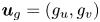 $\boldsymbol {u}_{g}=(g_{u},g_{v})$ is the velocity on the boundary
 $\partial \varOmega$ and
 $\boldsymbol {n}$ is the outward normal vector to
 $\varOmega$. Assuming
 $\partial \varOmega$ is closed, the boundary velocity needs to satisfy
 $\int _{\partial \varOmega }\boldsymbol {u}_{g}\boldsymbol {\cdot }\boldsymbol {n}\,{\mathrm d}S=0$. Further, the contact angle
 $\theta$ is the static contact angle between the fluid–fluid interface and the physical boundary. This form of the boundary condition (2.40) was derived in Jacqmin (Reference Jacqmin1999) (see also Gránásy et al. (Reference Gránásy, Pusztai, Saylor and Warren2007), Do-Quang & Amberg (Reference Do-Quang and Amberg2009) and Aland et al. (Reference Aland, Lowengrub and Voigt2010) in the context of the DD method). In particular, for an interface in equilibrium, a contact angle condition (Young's law) may be posed:
 $\cos (\theta )=(({\sigma _{2S}-\sigma _{1S}})/{\sigma })$, where
 $\theta$ is the (equilibrium) contact angle and
 $\sigma _{iS}$ is the interfacial energy between the solid and component
 $i$. The contact angle characterizes the wettability of the surface with
 $\theta =0$ denoting complete wetting. However, in the dynamical setting with the no-slip condition, the force needed to move a contact line is infinite making it necessary to regularize the system. Numerous methods have been implemented to regularize the problem including introducing a slip velocity, microscopic interactions, a precursor film or a diffuse interface.
Recently, two other quasi-incompressible two-fluid models have been presented in Gong et al. (Reference Gong, Zhao and Wang2017) and Shokrpour Roudbari et al. (Reference Shokrpour Roudbari, Şimşek, van Brummelen and van der Zee2018), where a different phase variable  $\phi$ is introduced leading to a different Cahn–Hilliard free energy and different systems of equations. In the paper by Shokrpour Roudbari et al. (Reference Shokrpour Roudbari, Şimşek, van Brummelen and van der Zee2018), in order to ensure the energy conservation for both the model equations and the corresponding numerical method, they introduced a dual-density form (two formulations of the variable density of the mixture) to the modelling framework. These two forms of the density appear in the model simultaneously and cannot be used interchangeably, leading to an extra mass conservation equation that needs to be solved along with the model equations. Our model equations are more compact and satisfy the energy conservation naturally. There is only one form of the variable density, and no extra mass conservation equation. In the paper by Gong et al. (Reference Gong, Zhao and Wang2017), the modelling framework they follow is based on the free energy dissipation which means that the framework is mainly focused on the isothermal case. Our modelling framework is more general, as the total energy, free energy and entropy can be introduced to the system in a thermodynamically consistent way, so that we can derive more general models to simulate the non-isothermal case or two-phase flows with non-uniform surface tension (surface tension gradient induced by the gradient of temperature or concentration of surfactants). Moreover, in their modelling framework, they did not provide the specific formulation for the Cahn–Hilliard free energy, which shortens the model derivation. However, to ensure the mass conservation of the fluid mixture and each fluid component, a parameter ‘
 $B$’ is introduced to the Cahn–Hilliard equation, serving as the coefficient of the mobility of the chemical potential. In their work, the calculation of ‘
 $B$’ seems quite long and complicated, and the resulting ‘
 $B$’ also makes the model equations more complicated compared to our model.
3. Diffuse domain reformulation: q-NSCH-DD
We next assume that the domain  $\varOmega$ has a complex boundary
 $\partial \varOmega$. To solve the q-NSCH model (2.34)–(2.40) numerically, we extend the results in Aland et al. (Reference Aland, Lowengrub and Voigt2010) and propose a DD approximation of the q-NSCH model in a larger and simpler domain
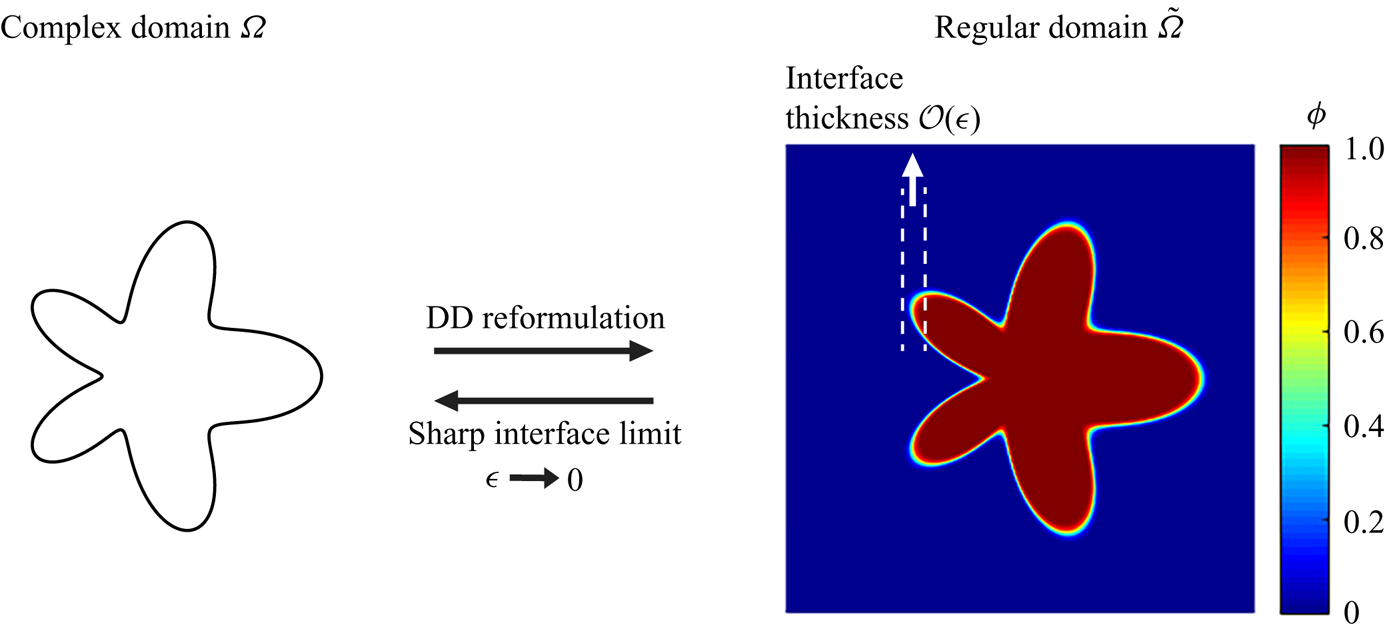
 $\tilde {\varOmega }$ (see figure 1). The q-NSCH-DD model is
 \begin{align} \rho(\phi\boldsymbol{u})_{t}+\rho \boldsymbol{u} \boldsymbol{\cdot}\boldsymbol{\nabla}( \phi\boldsymbol{u}) &=-\phi\boldsymbol{\nabla} p+\phi\boldsymbol{\nabla} \boldsymbol{\cdot}(\nu\boldsymbol{\nabla}\boldsymbol{u}) + \frac{1}{3}\phi\boldsymbol{\nabla}(\nu\boldsymbol{\nabla}\boldsymbol{\cdot} \boldsymbol{u}) + \frac{\tilde{\sigma}}{\epsilon_c}\phi\mu\boldsymbol{\nabla} c -\phi\rho g\boldsymbol{z}\nonumber\\ &\quad + BC_{\boldsymbol{u}}, \end{align}
 \begin{align} \boldsymbol{\nabla} \boldsymbol{\cdot}(\phi \boldsymbol{u})&= \boldsymbol{u}_{g}\boldsymbol{\cdot} \boldsymbol{\nabla}\phi + \alpha\boldsymbol{\nabla}\boldsymbol{\cdot} (M(c)\phi\boldsymbol{\nabla}\mu)+ \alpha^2\boldsymbol{\nabla}\boldsymbol{\cdot} (M(c)\phi\boldsymbol{\nabla}p) \nonumber\\ &\quad +BC_{\mu, p}, \end{align}
 \begin{equation} (\phi c)_{t}+ \boldsymbol{\nabla}\boldsymbol{\cdot }(\phi c\boldsymbol{u})= \boldsymbol{\nabla}\boldsymbol{\cdot}\left(\phi M(c) \boldsymbol{\nabla} \mu\right)+\alpha\boldsymbol{\nabla}\boldsymbol{\cdot} (M(c)\phi\boldsymbol{\nabla}p)+ BC_{\mu,p}, \end{equation}
 \begin{equation}\phi \mu= \phi \epsilon_c F'(c)-\epsilon_c^2 \boldsymbol{\nabla}\boldsymbol{\cdot} (\phi \boldsymbol{\nabla}c)+ BC_{c}, \end{equation}
with the boundary conditions  $\boldsymbol {u}=\boldsymbol {0}$,
 $\boldsymbol {n}\boldsymbol {\cdot }\boldsymbol {\nabla }c=\boldsymbol {n}\boldsymbol {\cdot }\boldsymbol {\nabla }(\mu +\alpha p)=0$ on
 $\partial \tilde {\varOmega }$. Note that the solution in
 $\varOmega$ is insensitive to the boundary conditions on
 $\partial \tilde {\varOmega }$ if
 $\partial \varOmega$ and
 $\partial \tilde {\varOmega }$ are sufficiently far apart (e.g. the distance between
 $\partial \varOmega$ and
 $\partial \tilde {\varOmega }$ is
 $\geqslant 10\epsilon$; Yu et al. (Reference Yu, Guo and Lowengrub2020)). Here the DD function
 $\phi$, given by
 \begin{equation} \phi(\boldsymbol{x},t)=0.5\left(1-\tanh\left(\frac{3r\left(\boldsymbol{x},t\right)}{\epsilon}\right)\right), \end{equation}
is used to approximate the characteristic function of the original domain  $\varOmega$. The function
 $r(\boldsymbol {x},t)$ is the signed distance to
 $\partial \varOmega$ (
 $r<0$ inside
 $\varOmega$) and
 $\epsilon$ is the thickness of the DD boundary. We fix
 $\epsilon _{c}$ and let
 $\epsilon \rightarrow 0$ unless otherwise stated. The reformulated
 $BC_{*}$ are used to enforce the original boundary conditions (2.38)–(2.40) on
 $\partial \varOmega$. In particular,
 \begin{gather} BC_{\boldsymbol{u}}=-\frac{1-\phi}{\epsilon^2}(\boldsymbol{u}-\boldsymbol{u}_{g}), \end{gather}
 \begin{gather}BC_{\mu,p}=0, \end{gather}
 \begin{gather}BC_{c} = -\frac{\epsilon_c|\nabla \phi|}{\sqrt{2}}\cos(\theta)(1-c)c. \end{gather}
Here, we extend  $\boldsymbol {u}_{g}$ into
 $\tilde {\varOmega }$ constantly in the normal direction. The advantage of the q-NSCH-DD system is that it is posed on a regular domain and can be solved by any standard approach (e.g. finite difference, finite element). In appendix A, we show that the q-NSCH-DD system (3.1)–(3.4) asymptotically converges to the original q-NSCH system (2.34)–(2.37) with boundary conditions (2.38)–(2.40) as
 $\epsilon \rightarrow 0$. Moreover, the numerical methods and the corresponding implementation are shown in appendix B.
Schematic of the DD method. The sharp (physical) interface domain  $\varOmega$ is embedded in a larger, square domain
 $\tilde {\varOmega }$ where a phase-field function
 $\phi$ approximates the characteristic function of the deposition domain.

4. Numerical results
4.1. Cavity flow
We first consider a two-phase fluid flow in a driven cavity (Boyer Reference Boyer2002). The numerical results from the q-NSCH system (2.34)–(2.37) on the physical domain  $\varOmega = [0,1]^2$ are compared to those from the q-NSCH-DD system (3.1)–(3.4) on an extended domain
 $\tilde \varOmega = [-0.25,1.25]^2$. For the original q-NSCH system, the boundary conditions on
 $\partial \varOmega$ are imposed as
 \begin{gather} \boldsymbol{u}= \boldsymbol{u}_{g}, \end{gather}
 \begin{gather}\boldsymbol{n}\boldsymbol{\cdot} \boldsymbol{\nabla}(\mu+\alpha p)=0, \end{gather}
 \begin{gather}\boldsymbol{n}\boldsymbol{\cdot} \boldsymbol{\nabla}c= 0, \end{gather}
where  $\boldsymbol {u}_{g}=(g_{u},g_{v})=(g_{u},0)$, and
 \begin{equation} g_{u} = \begin{cases} {\max} \left(0, 1-4 \times (x-0.5)^2\right) , & y=1 \\ 0, & y<1. \end{cases} \end{equation}
For the q-NSCH-DD system, the function  $\phi$, given by
 \begin{align} \phi&=0.5\left(1+\tanh {\left( \frac{3x}{\epsilon}\right)}\right) \times 0.5\left(1+\tanh {\left( \frac{3(1-x)}{\epsilon}\right)}\right)\nonumber\\ &\quad \times0.5\left(1+\tanh {\left( \frac{3y}{\epsilon}\right)}\right) \times 0.5\left(1+\tanh {\left( \frac{3(1-y)}{\epsilon}\right)}\right), \end{align}
is used to approximate the characteristic function of  $\varOmega$, and
 $g_{u}$ is extended to
 $\tilde \varOmega$ as follows:
 \begin{equation} g_{u} = \begin{cases} {\max} \left(0, 1-4 \times (x-0.5)^2\right) , & y\geqslant 1-\epsilon \\ 0, & y<1-\epsilon. \end{cases} \end{equation}
For both systems, the initial  $c$ is
 \begin{equation} c=\frac{1}{2}\left( 1- \tanh \left(\frac{0.5-y}{2\sqrt{2}\epsilon_c}\right)\right), \end{equation}
such that  $c=0$ for the fluid at the bottom and
 $c=1$ for the top fluid. In addition, we set
 \begin{align} \rho_{1}=\rho_{2}=1,\quad \nu_{1}=\nu_{2}=0.002,\quad g=0,\quad \tilde{\sigma} = 0,\quad \theta = 90^{\circ}\quad {\mathrm{and}}\quad \epsilon_c= 0.05. \end{align}
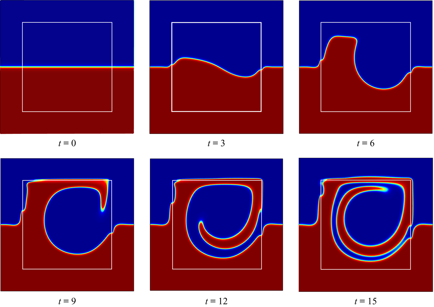
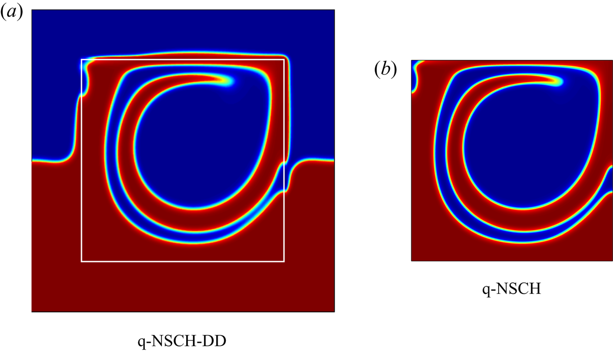
We present the evolution of the phase-field variable  $c$ obtained from the q-NSCH-DD system in figure 2 and compare
 $c$ at
 $t=15$ with the one from the q-NSCH system at the same time in figure 3.
Evolution of the phase-field variable  $c$ in a cavity flow. The results are obtained using the q-NSCH-DD system with a grid size
 $h=1.5/256$,
 $\textrm {d}t = 2.5\times 10^{-3}$ and
 $\epsilon =0.025$ in
 $\tilde \varOmega$. The white box represents the physical domain
 $\varOmega$.

Comparisons between the phase-field variable obtained from the q-NSCH-DD system (a) and that from the q-NSCH system (b) at  $t=15$. The white box in (a) marks the physical domain
 $\varOmega$.

Moreover, we compare the results between the q-NSCH and q-NSCH-DD solutions to test the convergence of the q-NSCH-DD system as  $\epsilon \rightarrow 0$. In particular, we use the results, including the velocities
 $u_{exc}$,
 $v_{exc}$, and phase variable
 $c_{exc}$, from the q-NSCH system with a grid size
 $h=1/1024$ and a time step
 $\textrm {d}t=3.90625\times 10^{-5}$ as the exact solutions. For the q-NSCH-DD system, we obtain the corresponding numerical solutions
 $u_\epsilon$,
 $v_\epsilon$ and
 $c_\epsilon$ using different values of
 $\epsilon$, namely
 $0.1$,
 $0.05$,
 $0.025$,
 $0.0125$,
 $0.00625$. We start with a grid size
 $h = 1.5/64$ and time step
 $\textrm {d}t=10^{-2}$ and
 $\epsilon =0.1$, and refine them together. For each
 $\epsilon$, we restrict the solutions from q-NSCH-DD to the original domain
 $\varOmega$ (see the smaller region bounded by the white solid line in figure 2) and compute the
 $L^2$ (
 $E^{(2)}$) and
 $L^\infty$ (
 $E^{(\infty )}$) errors as
 \begin{equation} E_{y}^{(2)}=||y_\epsilon-y_{exc}||_{L^{2}(\varOmega)}\quad \textrm{and}\quad E_{y}^{(\infty)}=||y_\epsilon-y_{exc}||_{L^{\infty}(\varOmega)}, \end{equation}
where  $y_\epsilon$ represents
 $u_\epsilon$,
 $v_\epsilon$,
 $c_\epsilon$ and
 $y_{exc}$ represents
 $u_{exc}$,
 $v_{exc}$,
 $c_{exc}$. Note that
 $E_{y}^{(\infty )}$ is computed where
 $\phi \geqslant 0.5$. The errors at
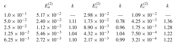
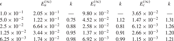
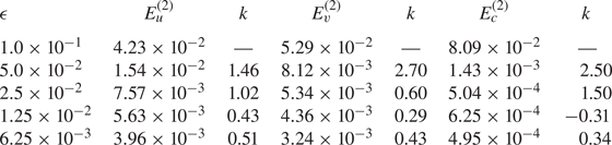
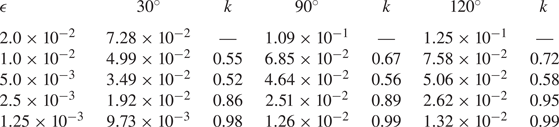
 $t=0.1$ are presented in tables 1 and 2. We observe that our DD approximation converges to the q-NSCH model with
 $\mathcal {O}(\epsilon )$.
Remark Another choice of  $BC_u = -\epsilon ^{-3}(1-\phi )(\boldsymbol {u}-\boldsymbol {u_g})$ was presented by Li et al. (Reference Li, Lowengrub, Rätz and Voigt2009) and later the scheme was shown to be
 $\mathcal {O}(\epsilon \ln (\epsilon ))$ accurate by Yu et al. (Reference Yu, Guo and Lowengrub2020). We here provide the numerical results using
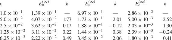
 $BC_u = -\epsilon ^{-3}(1-\phi )(\boldsymbol {u}-\boldsymbol {u}_{\boldsymbol {g}})$ for the cavity flow example in tables 3 and 4. This form of the velocity boundary condition was also used by Aland et al. (Reference Aland, Lowengrub and Voigt2010). The numerical set-up is identical to that considered above. We find that the errors are of a similar order of magnitude but are larger than those using
 $BC_u = -\epsilon ^{-2}(1-\phi )(\boldsymbol {u}-\boldsymbol {u}_{\boldsymbol {g}})$ and are sub-first-order accurate, which is consistent with the results of Yu et al. (Reference Yu, Guo and Lowengrub2020). In the following, we use
 $BC_u = -\epsilon ^{-2}(1-\phi )(\boldsymbol {u}-\boldsymbol {u}_{\boldsymbol {g}})$ exclusively. Moreover, our numerical results agree with the convergence results shown in Franz et al. (Reference Franz, Roos, Gärtner and Voigt2012).
The  $L^2$ errors and convergence rate (
 $k$) of the velocities
 $u$,
 $v$ and phase-field variable
 $c$ with different values of
 $\epsilon$ in a cavity flow in § 4.1. Here
 $k$ stands for the convergence rate. See text for details.

The  $L^\infty$ errors and convergence rate (
 $k$) of the velocities
 $u$,
 $v$ and phase-field variable
 $c$ in a cavity flow in § 4.1. Here
 $k$ stands for the convergence rate. See text for details.

The  $L^2$ errors and convergence rate (
 $k$) of the velocities
 $u$,
 $v$ and phase-field variable
 $c$ in a cavity flow using another choice of
 $BC_u = -\epsilon ^{-3}(1-\phi )(\boldsymbol {u}-\boldsymbol {u_g})$. See the remark in § 4.1 for details.

The  $L^\infty$ errors of the velocities
 $u$,
 $v$ and phase-field variable
 $c$ in a cavity flow using another choice of
 $BC_u = -\epsilon ^{-3}(1-\phi )(\boldsymbol {u}-\boldsymbol {u_g})$. See the remark in § 4.1 for details.

4.2. Droplet spreading
In order to test the accuracy of the q-NSCH-DD system with the moving contact line, we consider an example of a water droplet spreading on a flat substrate. In particular, we assume that there is a water droplet in the air, and is placed above a flat substrate. Due to the effect of gravity, the droplet falls down and spreads on the substrate. For the original q-NSCH system, the computational domain is  $\varOmega =[0,1]^2$ with the following boundary conditions on
 $\partial \varOmega$:
 \begin{gather} \boldsymbol{u}= 0\quad (\textrm{no slip}), \end{gather}
 \begin{gather}\boldsymbol{n}\boldsymbol{\cdot} \boldsymbol{\nabla}(\mu+\alpha p)=0\quad (\textrm{no flux}), \end{gather}
 \begin{gather}\boldsymbol{n}\boldsymbol{\cdot} \boldsymbol{\nabla}c= \frac{1}{\epsilon_c\sqrt{2}}\cos (\theta) (1-c)c\quad (\textrm{contact angle}). \end{gather}
For the q-NSCH-DD system, we extend the computational domain to  $\tilde {\varOmega }=[-0.25,1.25]^2$ with the following boundary conditions on
 $\partial \tilde {\varOmega }$:
 \begin{gather} \boldsymbol{u}= 0\quad (\textrm{no slip}), \end{gather}
 \begin{gather}\boldsymbol{n}\boldsymbol{\cdot} \boldsymbol{\nabla}(\mu+\alpha p)=0\quad (\textrm{no flux}), \end{gather}
 \begin{gather}\boldsymbol{n}\boldsymbol{\cdot} \boldsymbol{\nabla}c= 0\quad (\textrm{no flux}). \end{gather}
Moreover, we use the function  $\phi$, given by
 \begin{align} \phi&=0.5\left(1+\tanh {\left( \frac{3x}{\epsilon}\right)}\right) \times 0.5\left(1+\tanh {\left( \frac{3(1-x)}{\epsilon}\right)}\right)\nonumber\\ &\quad \times 0.5\left(1+\tanh {\left( \frac{3y}{\epsilon}\right)}\right)\times 0.5\left(1+\tanh {\left( \frac{3(1-y)}{\epsilon}\right)}\right), \end{align}
to approximate the characteristic function of  $\varOmega$. For both systems, the initial condition for the phase variable
 $c$ is given by
 \begin{equation} c=\frac{1}{2}\left( 1- \tanh \left(\frac{r-0.2}{2\sqrt{2}\epsilon_c}\right)\right), \end{equation}
with  $r=\sqrt {(x-0.5)^2+(y-0.21)^2}$, such that
 $c=0$ for the water droplet and
 $c=1$ for the air. In addition, we set
 \begin{align} \left.\begin{gathered} \rho_{1}=1,\quad \rho_{2}=1000,\quad \nu_{1}=0.1,\quad \nu_{2}=10,\quad g=0.98, \quad \tilde{\sigma} = 10,\quad \theta = 60^{\circ},\\ \epsilon= 0.0025\quad {\mathrm{and}}\quad \epsilon_c= 0.005. \end{gathered}\right\} \end{align}
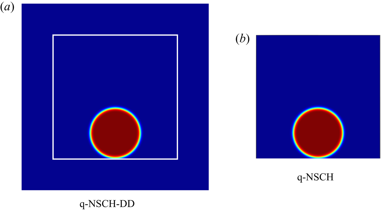
In figure 4, we show the domains  $\tilde {\varOmega }$ and
 $\varOmega$ together with the initial
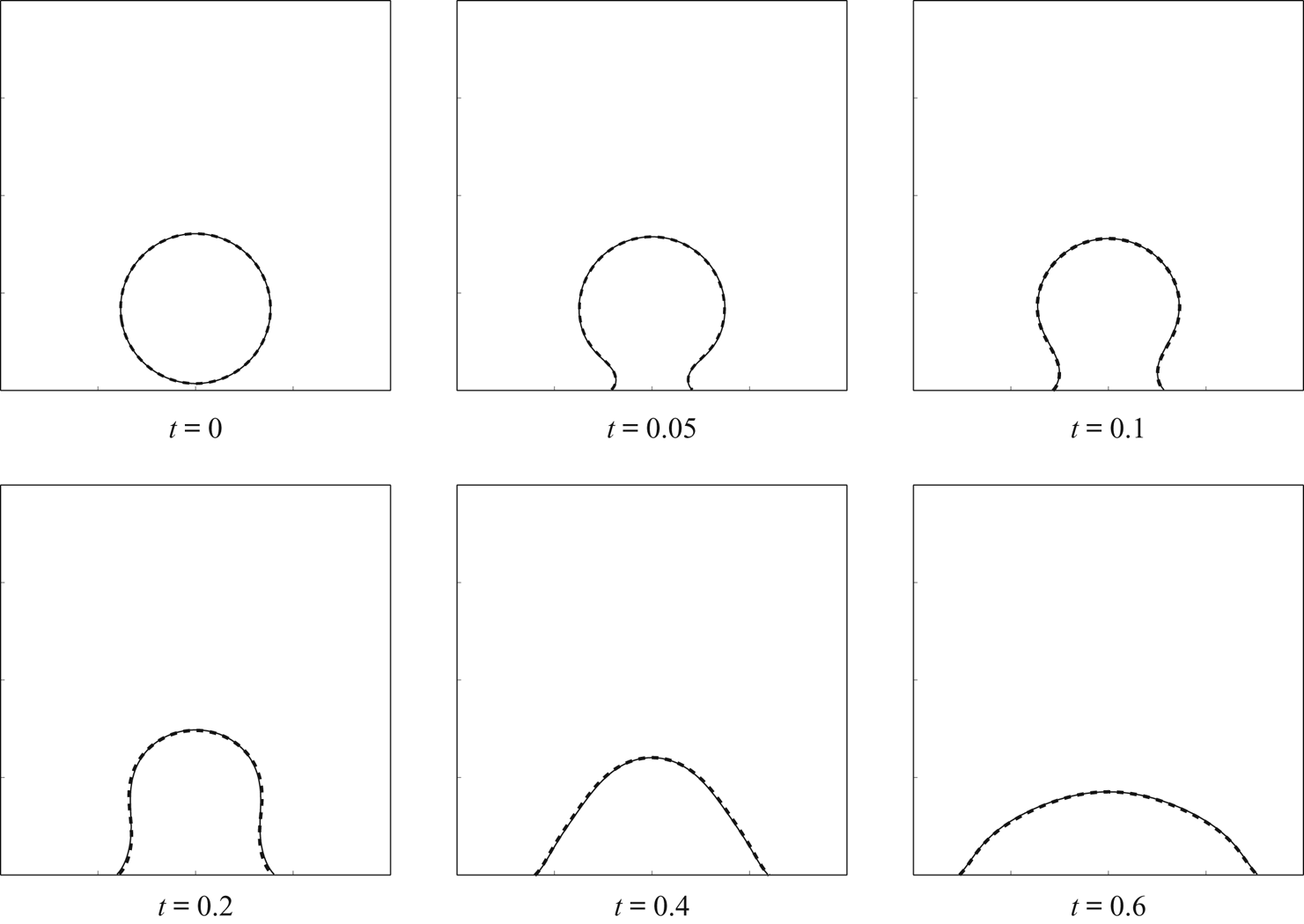
 $c$ for both systems. In figure 5, we show the dynamics of the contact line of the moving droplet, where the solid (dotted) lines represent the contour line (
 $c=0.5$) of the numerical results obtained from the q-NSCH (the q-NSCH-DD) system. A good agreement can be observed between the two results. Again, we compare the results obtained from the two systems, and test the convergence rate of the q-NSCH-DD system as
 $\epsilon \rightarrow 0$. As in the previous section, we use the results of phase variable
 $c_{exc}$ from the q-NSCH system with agrid size
 $h=1/1024$ and a time step
 $\textrm {d}t=3.90625\times 10^{-5}$ as the exact solutions. For the q-NSCH-DD system, we obtain the corresponding numerical solutions
 $c_\epsilon$ using different values of
 $\epsilon$, namely
 $0.1$,
 $0.05$,
 $0.025$,
 $0.0125$,
 $0.00625$. We start with a grid size
 $h = 1.5/64$ and time step
 $\textrm {d}t=10^{-2}$ and
 $\epsilon =0.1$, and refine them together. For each
 $\epsilon$, we restrict the solutions from q-NSCH-DD to the original domain
 $\varOmega$ and compute the
 $L^2$ (
 $E^{(2)}$) and
 $L^\infty$ (
 $E^{(\infty )}$) errors as shown in (4.9a,b). The errors at
 $t=0.1$ are presented in table 5, where we observe that our DD approximation converges to the q-NSCH system with
 $\mathcal {O}(\epsilon )$.
The computational domain for the q-NSCH-DD system (a) and the q-NSCH system (b), and the initial condition for phase variable  $c$. The white box in (a) marks the physical domain
 $\varOmega$.

The dynamics of moving contact line of a water droplet on a solid substrate, where the solid (dotted) lines are the contour lines ( $c=0.5$) of the numerical results obtained from the q-NSCH (q-NSCH-DD) system.

The  $L^2$ and
 $L^{\infty }$ errors and convergence rate (
 $k$) of the phase-field variable restricted on
 $\varOmega$,
 $\phi c$, at time
 $t=0.1$ with contact angle
 $\theta = 60^{\circ }$. See § 4.2 for details.

4.3. Droplet on cylinder
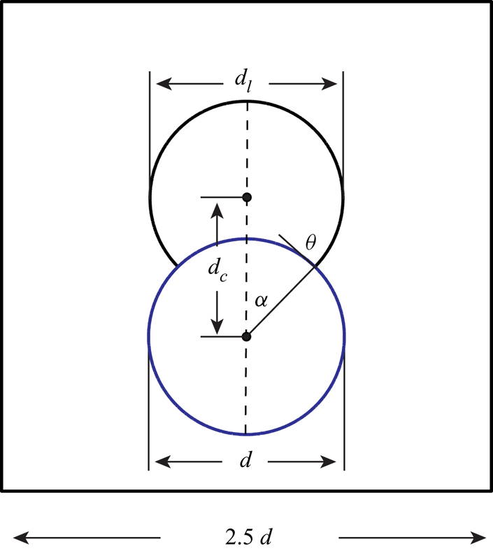
We next consider a circular droplet of diameter  $d$ wetting and dewetting on a solid cylinder. Initially, the droplet is placed on the cylinder of the same diameter
 $d$ with contact angle
 $\theta _{0}=90^{\circ }$ (see figure 6). We mention that careful studies for wetting and dewetting phenomena using a phase-field model have been presented in Gránásy et al. (Reference Gránásy, Pusztai, Saylor and Warren2007), Dziwnik, Münch & Wagner (Reference Dziwnik, Münch and Wagner2017) and Rainer et al. (Reference Rainer, Steven, Marco and Axel2019). With
 $\theta$ being the static contact angle, the contact line of the droplet recedes if
 $\theta <\theta _{0}$ or spreads if
 $\theta >\theta _{0}$, and eventually reaches an equilibrium with the interface intersecting the solid cylinder at an angle of
 $\theta$. In the absence of gravity, the equilibrium state of the droplet can be obtained analytically by carving the cylinder out of a circle (Liu & Ding Reference Liu and Ding2015; O'Brien & Bussmann Reference O'Brien and Bussmann2018); see figure 7. The distance between the centres of the droplet and the cylinder,
 $d_{c}$, and the diameter of the circle,
 $d_{l}$, can be computed by solving
 \begin{gather} \pi d^2/4=(\alpha + \theta )(d_{l}/2)-\alpha(d/2)^2+(d_{l}d/4)\sin{\theta}, \end{gather}
 \begin{gather}d_{l}=d\cos{\theta}+\sqrt{d^{2}\cos^2{\theta}-d^2+4d_{c}^{2}}, \end{gather}
where
 \begin{equation} \alpha=\arccos{\left(\frac{d^{2}+4d_{c}^{2}-d^{2}_{l}}{4d d_{c}}\right)}.\end{equation}
The exact solution  $c_{exc}$ is given by
 \begin{equation} c_{exc}=\frac{1}{2}\left( 1+ \tanh \left(\frac{r_{exc}-0.5d_{l}}{2\sqrt{2}\epsilon_c}\right)\right) \end{equation}
and  $r_{exc}=\sqrt {(x-1.25d)^2+(y-0.6d-d_{c})^2}$. To apply the q-NCSH-DD system, we extend
 $\varOmega$ to a larger domain
 $\tilde \varOmega$ =
 $[0,2.5d]\times [0,2.5d]$. The initial
 $\phi$ and
 $c$ are given by
 \begin{equation} \left.\begin{gathered} \phi=\frac{1}{2}\left( 1+\tanh \left(\frac{3(r_{\phi}-0.5d)}{\epsilon}\right)\right),\\ c=\frac{1}{2}\left( 1+ \tanh \left(\frac{r_c-0.5d}{2\sqrt{2}\epsilon_c}\right)\right),\end{gathered}\right\} \end{equation}
where  $r_{\phi }\!=\!\sqrt {(x\!-\!1.25d)^2\!+\!(y\!-\!0.6d)^2}$ and
 $r_c\!=\!\sqrt {(x\!-\!1.25d)^2\!+\!(y\!-\!0.6d\!-\!0.5\sqrt {2}d)^2}$, such that
 $c=1$ for the droplet (indicated by 1) and
 $c=0$ for the surrounding fluid medium (indicated by 2). All the other parameters are set as follows:
 \begin{equation} \left.\begin{gathered} \rho_{1}=1000\ (\mathrm{droplet}),\quad \rho_{2}=1\ (\mathrm{air}), \quad\nu_{1}=0.1,\quad \nu_{2}=0.001,\quad \tilde{\sigma}=1, \\ g=0,\quad \epsilon_c=\epsilon,\quad d=1. \end{gathered}\right\} \end{equation}
Set-up for droplet on cylinder.

Comparisons between the numerical results at equilibrium (solid lines) and the analytic solutions (dashed lines) with different static contact angles, where the angles are indicated inside the blue cylinders. See text for details.

We solve the q-NSCH-DD system with different values of  $\epsilon$ (
 $=\epsilon _{c}$) and various
 $\theta$ (
 $=30^\circ , 90^\circ ,120^\circ$) to obtain the numerical solutions
 $c$ at equilibrium and then compare with the corresponding analytical solutions
 $c_{exc}$ in both
 $L^2$ and
 $L^{\infty }$ norm:
 \begin{equation} E_{c}^{(2)}=||c-c_{exc}||_{L^{2}(\varOmega)}\quad \textrm{and} \quad E_{c}^{(\infty)}=||c-c_{exc}||_{L^{\infty}(\varOmega)}. \end{equation}
We start with a grid size  $h=2.5/128$, a time step
 $\textrm {d}t=0.01$ and
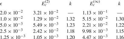
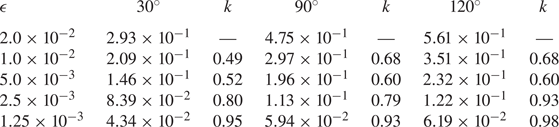
 $\epsilon =\epsilon _c=0.02$ and conduct the error analysis by refining them together. In tables 6 and 7, we present the
 $L^2$ and
 $L^\infty$ errors and find that our q-NSCH-DD system provides a first-order approximation to the exact solution (sharp interface).
The  $L^2$ errors and convergence rate (
 $k$) of the phase-field variable restricted on
 $\varOmega$,
 $\phi c$, at equilibrium with different static contact angles
 $30^{\circ }$,
 $90^{\circ }$ and
 $120^{\circ }$.

The  $L^{\infty }$ errors of the phase-field variable restricted on
 $\varOmega$,
 $\phi c$, at equilibrium with different static contact angles
 $30^{\circ }$,
 $90^{\circ }$ and
 $120^{\circ }$. See text for details.

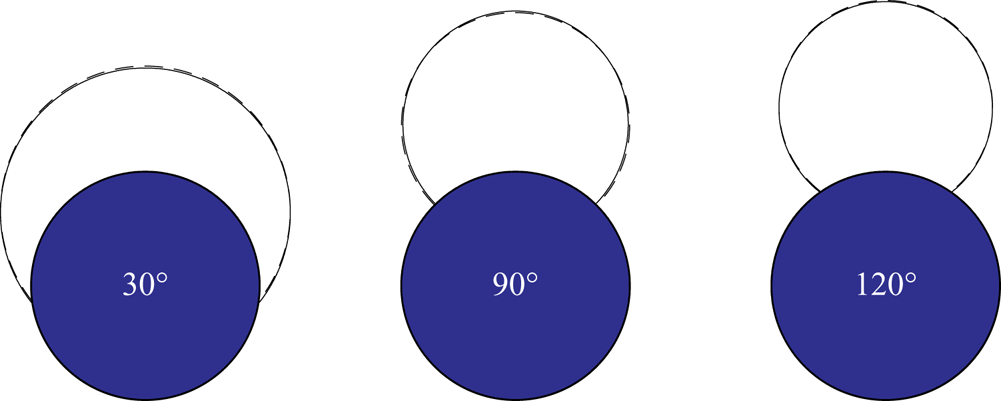
In figure 7, we also present the numerical solutions  $\phi c$ with analytical solutions at equilibrium from the q-NSCH-DD system with various
 $\theta$ (
 $=30^{\circ }, 90^\circ ,120^\circ$). The analytical solutions are the dashed curves. Here the grid size is
 $n=2048$ and
 $\epsilon =\epsilon _{c}=0.00125$. There is excellent agreement between the numerical and analytical solutions.
4.4. Penetration of a liquid droplet into porous media
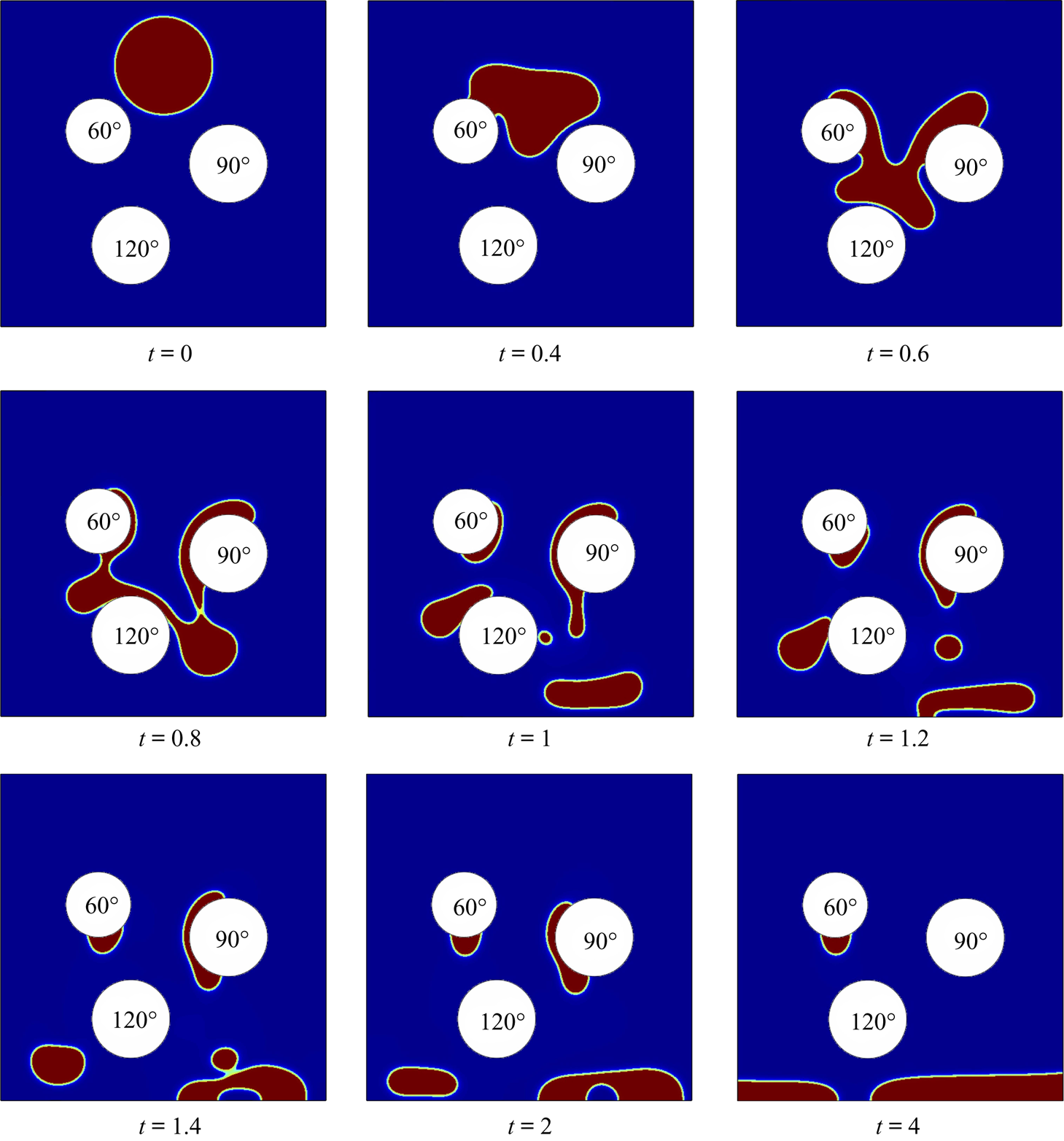
As a final test, we consider a two-dimensional droplet falling through a porous substrate consisting of three cylinders ( $C_i$,
 $i=1,2,3$) with different wettabilities, as shown in figure 8. We also fix the contact angle of the fluid–fluid interface at the walls to be
 $90^{\circ }$. The extended domain
 $\tilde \varOmega = [0,1]\times [0,1]$ is discretized on a uniform mesh of
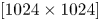 $[1024\times 1024]$. The original physical domain is
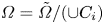 $\varOmega = \tilde \varOmega /(\cup C_i)$. There are three cylinders in the domain with radii
 $r_1=0.1$,
 $r_2=0.12$,
 $r_3=0.15$, and centres
 $(0.3,0.6)$,
 $(0.4,0.25)$,
 $(0.7,0.5)$, respectively. Initially, a heavy liquid drop with radius
 $r_d=0.15$ is placed above the cylinders with the centre
 $(0.5,0.8)$. Note that the initial
 $\phi$ and
 $c$ can be given by a slight modification of (4.23). Again, we let
 $c=1$ stand for the heavy fluid droplet and
 $c=0$ stands for the light fluid medium. All other parameters are set as follows:
 \begin{equation} \left.\begin{gathered} \rho_{1}=1000,\quad \rho_{2}=1,\quad\nu_{1}=10,\quad\nu_{2}=0.1,\quad g=1,\quad\tilde{\sigma}=1,\\ \epsilon_c=0.001,\quad\epsilon=0.002. \end{gathered}\right\} \end{equation}
The dynamics of droplet impact is shown in figure 8 via snapshots at different times. Initially, the droplet starts moving downwards due to gravitational forces. Dramatic deformations are observed when the droplet comes into contact with the left and right cylinders. After impacting on the cylinder at the bottom, the droplet splits into several parts. In the end, it is interesting to see that there is no liquid on the cylinders with contact angle of  $\theta =90^{\circ }$ and
 $\theta =120^{\circ }$. All the liquid rests either on the cylinder with
 $\theta =60^{\circ }$ or on the walls.
Snapshots of the penetration of a liquid droplet into porous media with different static contact angles, where the angles are indicated inside the white cylinders.

4.5. Moving domains
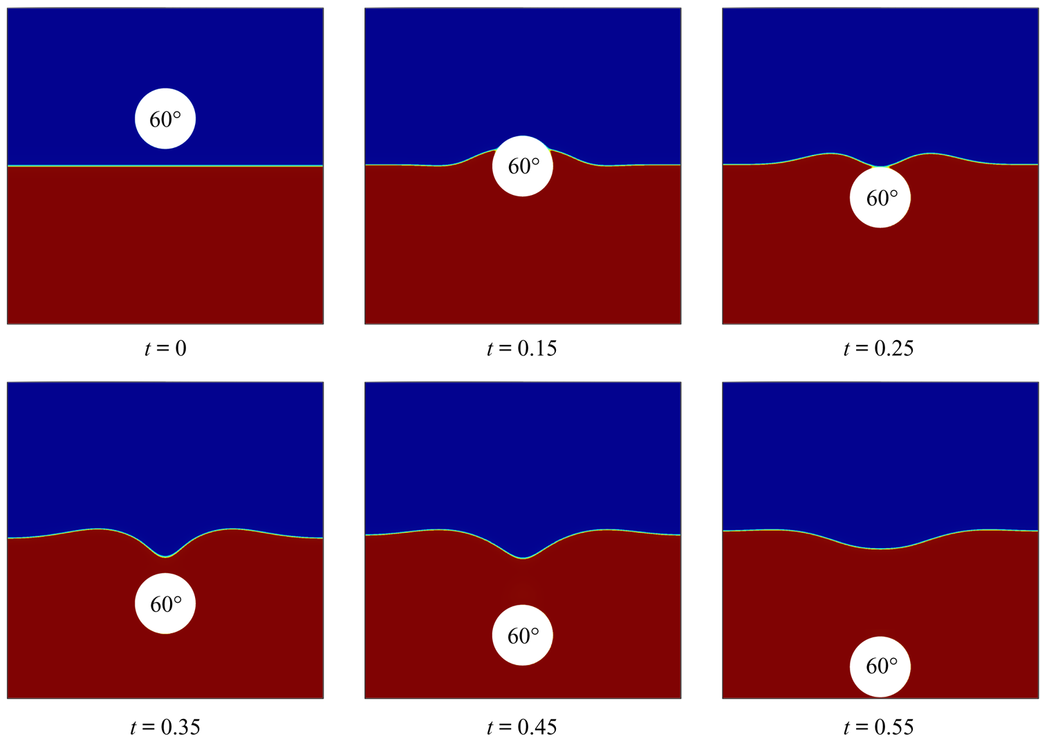
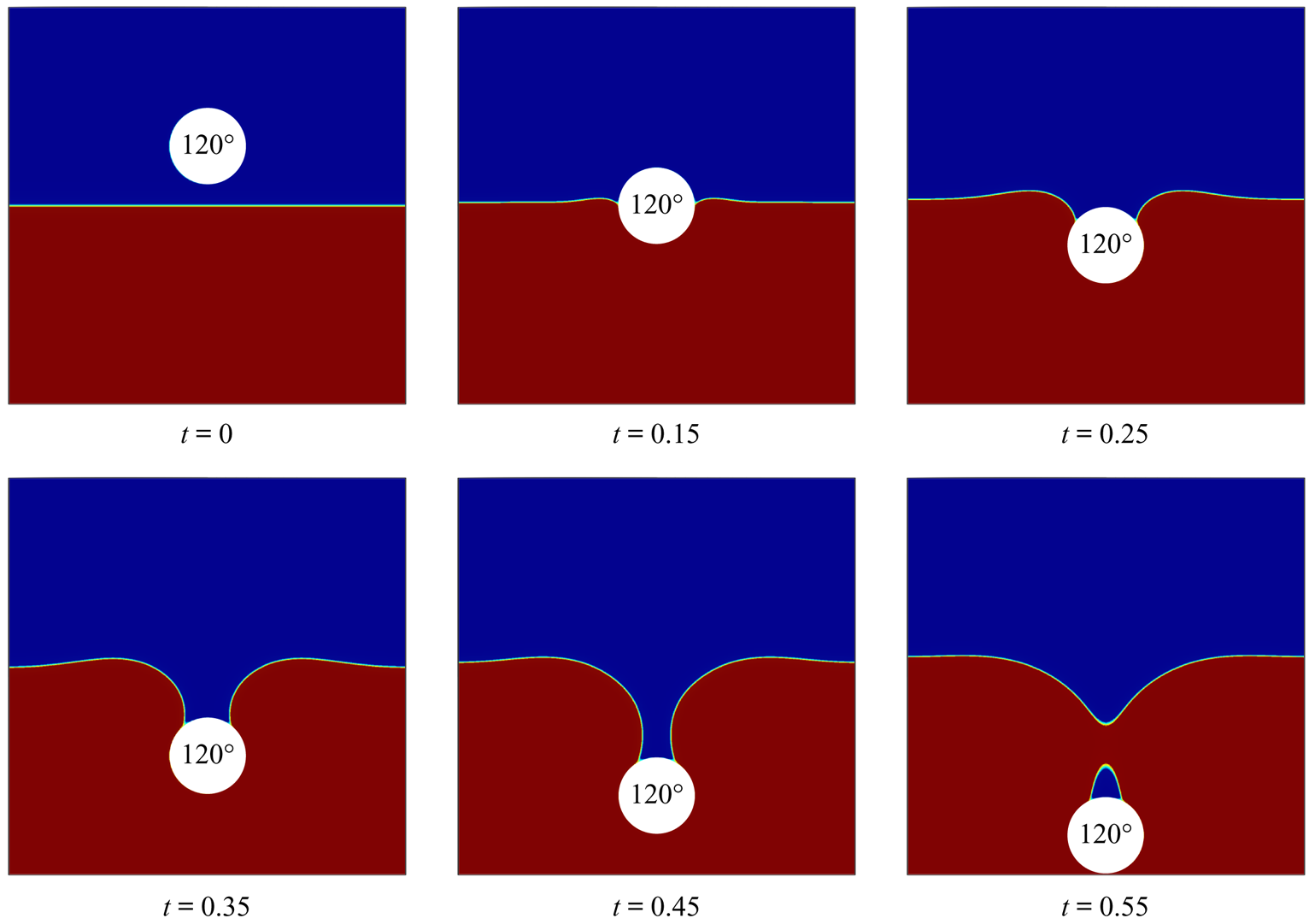
In the next example, we simulate solid hydrophobic and hydrophilic balls impacting an air–water interface in two dimensions. The extended domain is  $\tilde {\varOmega }=[0,1]\times [0,1]$, and the air is placed on top of the water, with a flat interface at
 $y=0.5$. Figure 9 shows the initial
 $\phi$ (the complex domain) and
 $c$ (the air–water interface), which are given by
 \begin{equation} \left.\begin{gathered} \phi=\frac{1}{2}\left( 1+\tanh \left(\frac{3(r_{\phi}-0.1)}{\epsilon}\right)\right),\\ c=\frac{1}{2}\left( 1- \tanh \left(\frac{y-0.5}{2\sqrt{2}\epsilon_c}\right)\right), \end{gathered}\right\} \end{equation}
where  $r_{\phi }=\sqrt {(x-0.5d)^2+(y-0.65d)^2}$ and such that
 $\phi =0$ for the solid ball (in white) and
 $\phi =0$ for the bulk regions with water (in red) or air (in blue). Here we assume that the ball moves with a constant velocity
 $\boldsymbol {v}_{ball}=(0,-1)$. All the other parameters are set as follows:
 \begin{equation} \left.\begin{gathered} \rho_{1}=1000\ (\mathrm{water}, \mathrm{lower\ fluid}),\quad \rho_{2}=1\quad (\mathrm{air}, \mathrm{upper\ fluid}),\quad \nu_{1}=0.1, \\ \nu_{2}=0.001,\quad \tilde{\sigma}=4,\quad g=0.98,\quad \epsilon_c=\epsilon=0.003. \end{gathered}\right\} \end{equation}
Two contact angle boundary conditions, namely  $\theta _{0}=60^{\circ }$ (hydrophilic) and
 $\theta _{0}=120^{\circ }$ (hydrophobic), are imposed at the boundary of the solid ball. Figures 9 and 10 show the results of the simulations. For the hydrophilic ball, the contact line moves continuously on the surface of the ball until reaching the ball peak, at which the liquid merges and detaches from the surface of the ball. In contrast, for the hydrophobic ball, the contact line initially moves along the ball surface, but eventually rests on the ball. As a consequence of the pinned contact line, the length of the air cavity keeps growing. A neck then appears at the cavity and breaks up, thereby generating a bubble attached at the top of the ball.
Snapshots of water entry of a hydrophilic ball with contact angle  $60^{\circ }$. Here the white region represents the solid falling ball, the blue region represents the air and the red region represents the water.

Snapshots of water entry of a hydrophobic ball with contact angle  $120^{\circ }$. Here the white region represents the solid falling ball, the blue region represents the air and the red region represents the water.

5. Discussion
A DD method was proposed to simulate two-phase flows with moving contact lines in complex geometries. We first derived a new thermodynamically consistent, locally mass conservative diffuse interface model, the q-NSCH system, for two-phase fluid flows with variable physical properties. We then combined this model with the DD method, to yield the q-NSCH-DD system in which a phase-field function  $\phi$ was introduced to approximate the characteristic function of the original complex domain. Moreover, the q-NSCH-DD system contains extra source terms to enforce the boundary conditions on the complex domain. In the sharp interface limit, we showed that the q-NSCH-DD system converged to the q-NSCH system as the thickness
 $\epsilon$ of the DD boundary shrinks to zero at an
 $\mathcal {O}(\epsilon )$ rate.
We solved the q-NSCH-DD system using an existing finite difference multigrid solver on a staggered grid. Using the DD formulation, the system was solved on a larger, regular domain without any modification of the solver. Numerical results confirmed that the solution to the q-NSCH-DD system converged to that of the q-NSCH system and to analytical solutions. In addition, we showed that the q-NSCH-DD system not only allowed the contact line to move on the curved boundaries, but also made the fluid–fluid interface intersect the solid object at an angle consistent with the prescribed contact angle.
In Yu et al. (Reference Yu, Guo and Lowengrub2020), the authors proposed that using a modified version of the boundary condition term  $BC_u = -\epsilon ^{-3}(1-\phi )(\boldsymbol {u}-\boldsymbol {u_g}-r\boldsymbol {n}\boldsymbol {\cdot }\boldsymbol {\nabla }\boldsymbol {u})$, where
 $r$ is the signed distance function to
 $\varOmega$, could achieve second-order accuracy in
 $L^2$ and 1.5-order accuracy in
 $L^\infty$, although this was only shown to be the case in problems in Yu et al. (Reference Yu, Guo and Lowengrub2020). In preliminary work, we implemented this form of the boundary condition but did not find the expected improvement in convergence rate. This is likely due to the vector form of the problem, and the quasi-incompressibility condition, which couples the derivatives of the velocity. In future work, we will extend the asymptotic analysis in § 4 and use the approach developed in Yu et al. (Reference Yu, Guo and Lowengrub2020) to guide the development of a higher-order-accurate version of the q-NSCH-DD system. Moreover, we will also consider dynamic contact angle formulations developed in Liu & Wu (Reference Liu and Wu2019). Since the DD formulation is dimension-independent, we also plan to develop a three-dimensional, spatially adaptive version of the solver.
Acknowledgements
J.L. acknowledges partial support from funding from the National Science Foundation-Division of Mathematical Sciences (NSFDMS) through grant DMS-1719960 and the Center for Multiscale Cell Fate Research at UC Irvine, which is supported by NSF-DMS (DMS-1763272) and the Simons Foundation (594598, QN). J.L. additionally acknowledges partial funding from the National Institutes of Health (NIH) through grant 1U54CA217378-01A1 for a National Center in Cancer Systems Biology at the University of California, Irvine, and NIH grant P30CA062203 for the Chao Comprehensive Cancer Center at the University of California, Irvine. S.W. acknowledges partial support from the NSFDMS through grants NSF-DMS 1719854 and NSF-DMS 2012634. P.L. acknowledges partial support from NSFC grant 11771040 and NSFC grant 11861131004.
Declaration of interests
The authors report no conflict of interest.
Appendix A. Asymptotic analysis of q-NSCH-DD
We use the method of matched asymptotic expansions to analyse the q-NSCH-DD system. In particular, we expand the variables in powers of the interface thickness in regions close to and far from the boundary. Parameter  $Y$ represents
 ${\boldsymbol {u}}$,
 $c$,
 $\mu$ or
 $p$. The two expansions are then matched in a region where both are valid. We assume
 $\partial {\varOmega }$ is smooth, but we are able to compute solutions accurately even if
 $\partial {\varOmega }$ has corners.
A.1. Outer expansions
On each side far from the domain boundary  $\partial {\varOmega }$, there exists an outer expansion, here labelled
 $\bar {Y}_1(\boldsymbol {x};\epsilon )$ where
 $r<0$ and
 $\phi =1$ (e.g. inside
 $\varOmega$), and
 $\bar {Y}_2(\boldsymbol {x};\epsilon )$ where
 $r>0$ and
 $\phi =0$ (e.g. outside
 $\varOmega$), where
 $\bar {Y}_i$ represents
 $\bar {\boldsymbol {u}}_i$,
 $\bar {c}_i$,
 $\bar {\mu }_i$ or
 $\bar p_i$. The outer expansion is away from
 $\partial \tilde \varOmega$. On the boundary of
 $\partial \tilde \varOmega$, we assume the following boundary conditions:
 ${\boldsymbol {n}}\boldsymbol {\cdot } {\boldsymbol {\nabla }} \bar {\boldsymbol {u}}_2=0$ and
 $\boldsymbol {n}\boldsymbol {\cdot } \boldsymbol {\nabla } \bar {p}_2=\boldsymbol {n}\boldsymbol {\cdot }\boldsymbol {\nabla } \bar {\mu }_2= \boldsymbol {n}\boldsymbol {\cdot } \boldsymbol {\nabla } \bar {c}_2=0$. We assume the outer solution
 $Y_1$ has a regular expansion
 \begin{equation} \bar{Y}_1(\boldsymbol{x};\epsilon)=\bar{Y}_1^{(0)}(\boldsymbol{x})+ \epsilon\bar{Y}_1^{(1)}(\boldsymbol{x})+\cdots,\quad i=1,2.\end{equation}
Plugging into (3.1)–(3.4), we obtain
 \begin{align} \rho(c^{(0)})\frac{\partial}{\partial_t}\bar{\boldsymbol{u}}_1^{(0)}+ \rho(c^{(0)})\bar{\boldsymbol{u}}_1^{(0)} \boldsymbol{\cdot}\boldsymbol{\nabla} \bar{\boldsymbol{u}}_1^{(0)} &=-\boldsymbol{\nabla} \bar{p}_1^{(0)}+\boldsymbol{\nabla} \boldsymbol{\cdot}(\nu\boldsymbol{\nabla}\bar{\boldsymbol u}_1^{(0)}) +\frac{1}{3} \boldsymbol{\nabla}(\nu\boldsymbol{\nabla}\boldsymbol{\cdot}\bar{\boldsymbol u}_1^{(0)}) \nonumber\\ &\quad + \frac{\tilde{\sigma}}{\epsilon_c}\bar{\mu}_1^{(0)}\boldsymbol{\nabla} \bar{c}_1^{(0)}-\rho g\boldsymbol{z}, \end{align}
 \begin{gather} \boldsymbol{\nabla} \boldsymbol{\cdot} \bar{\boldsymbol{u}}_1^{(0)}= \alpha\boldsymbol{\nabla}\boldsymbol{\cdot} (M(\bar{c}_1^{(0)})\boldsymbol{\nabla} \bar{\mu}_1^{(0)})+\alpha^2\boldsymbol{\nabla}\boldsymbol{\cdot} (M(\bar{c}_1^{(0)}) \boldsymbol{\nabla}\bar{p}_1^{(0)}), \end{gather}
 \begin{gather}\frac{\partial}{\partial_t}\bar{c}^{(0)}_{1}+\bar{\boldsymbol{u}}_1^{(0)} \boldsymbol{\cdot} \boldsymbol{\nabla} \bar{c}_1^{(0)}= \boldsymbol{\nabla}\boldsymbol{\cdot}\left( M(\bar{c}_1^{(0)}) \boldsymbol{\nabla} \bar{\mu}_1^{(0)}\right)+\alpha\boldsymbol{\nabla}\boldsymbol{\cdot} \left( M(\bar{c}_1^{(0)}) \boldsymbol{\nabla} \bar{p}_1^{(0)}\right), \end{gather}
 \begin{gather}\bar\mu_1^{(0)}= \epsilon_c F'(\bar{c}_1^{(0)})-\epsilon_c^2 \boldsymbol{\nabla}\boldsymbol{\cdot} (\boldsymbol{\nabla}\bar{c}_1^{(0)}). \end{gather}
Now, if  $\bar {\boldsymbol {u}}_1^{(0)}$,
 $\bar p_1^{(0)}$,
 $\bar \mu _1^{(0)}$ and
 $\bar {c}_1^{(0)}$ satisfy the corresponding boundary conditions on
 $\partial \varOmega$ so that they are the unique solutions to q-NSCH (2.34)–(2.37), then the q-NSCH-DD system recovers the q-NSCH model at leading order. Assuming a similar expansion for
 $\bar {Y}_2$, we obtain
 $\bar {\boldsymbol {u}}_2 = {\boldsymbol {u}}_g$,
 ${\boldsymbol {n}}\boldsymbol {\cdot } {\boldsymbol {\nabla }}\bar {p}_2={\boldsymbol {n}}\boldsymbol {\cdot } {\boldsymbol {\nabla }}\bar {\mu }_2={\boldsymbol {n}}\boldsymbol {\cdot } {\boldsymbol {\nabla }}\bar {c}_2=0$. The boundary conditions at
 $\partial \varOmega$ are obtained by matching the outer and inner expansions.
A.2. Inner expansions
For the inner expansions, we introduce a local coordinate system near the domain boundary  $\partial {\varOmega }$:
 \begin{equation} \boldsymbol{x}(\boldsymbol{s},z;\epsilon)=\boldsymbol{X}(\boldsymbol{s};\epsilon)+\epsilon z\boldsymbol{n}(\boldsymbol{s};\epsilon), \end{equation}
where  $\boldsymbol {X}(\boldsymbol {s};\epsilon )$ is a parametrization of the interface,
 $\boldsymbol {n}(\boldsymbol {s};\epsilon )$ is the interface normal vector that points out of
 $\varOmega$,
 $\boldsymbol {s}$ is the tangential vector and
 $z$ is the stretched variable given by
 \begin{equation} z=\frac{r(\boldsymbol{x})}{\epsilon}, \end{equation}
where  $r(\boldsymbol {x})$ is the signed distance function to
 $\partial \varOmega$. Note that
 $\lim _{z\rightarrow -\infty }\phi =1$ and
 $\lim _{z\rightarrow +\infty }\phi =0$. In the local coordinate system, the derivatives become
 \begin{gather} {\boldsymbol{\nabla}} = \frac{1}{\epsilon}\boldsymbol{n}\partial_z+\frac{1}{1+\epsilon z \kappa}{\boldsymbol{\nabla}}_s , \end{gather}
 \begin{gather}\varDelta =\frac{1}{\epsilon^2}\partial_{zz}+\frac{1}{\epsilon}\frac{\kappa}{1+\epsilon z \kappa}\partial_ z+\frac{1}{1+\epsilon z \kappa}{\boldsymbol{\nabla}}_s \boldsymbol{\cdot}\left(\frac{1}{1+\epsilon z \kappa}{\boldsymbol{\nabla}}_s\right), \end{gather}
 \begin{gather}\partial_t = -\frac{\boldsymbol{n}\boldsymbol{\cdot} \boldsymbol{u}}{\epsilon}\partial_z+o(1), \end{gather}
where  $\kappa = \boldsymbol {\nabla }_{\boldsymbol {s}}\boldsymbol {\cdot } \boldsymbol {n}$ is the total curvature of
 $\partial {\varOmega }$. We assume that the inner expansion is given by
 \begin{equation} \hat{Y}(z,\boldsymbol{s};\epsilon)=\hat{Y}^{(0)}(z,\boldsymbol{s})+\epsilon \hat{Y}^{(1)}(z,\boldsymbol{s})+\cdots,\end{equation}
where  $\hat {Y}$ represents
 $\hat {\boldsymbol {u}}$,
 $\hat {c}$,
 $\hat {\mu }$ and
 $\hat {p}$. In a region of overlap where both expansions are valid, we have
 \begin{gather} \bar{Y}_1(\boldsymbol{X}+\epsilon z \boldsymbol{n};\epsilon) \simeq \hat{Y}(z,\boldsymbol{s};\epsilon)\quad \mathrm{ as }~~z\rightarrow -\infty, \end{gather}
 \begin{gather}\bar{Y}_2(\boldsymbol{X}+\epsilon z \boldsymbol{n};\epsilon) \simeq \hat{Y}(z,\boldsymbol{s};\epsilon)\quad \mathrm{ as }~~z\rightarrow+\infty. \end{gather}
Combining (A 1), (A 11)–(A 13), we have the following asymptotic matching conditions at the first two leading orders:
 \begin{gather} \lim_{z\rightarrow-\infty}\hat{Y}^{(0)}(z,\boldsymbol{s})=\bar{Y}_1^{(0)}(\boldsymbol{s}), \end{gather}
 \begin{gather}\lim_{z\rightarrow-\infty}\hat{Y}^{(1)}(z,\boldsymbol{s})= \bar{Y}^{(1)}_1(\boldsymbol{s}) + z \boldsymbol{n} \boldsymbol{\cdot}\boldsymbol{\nabla} \bar{Y}^{(0)}_1, \end{gather}
 \begin{gather}\lim_{z\rightarrow+\infty}\hat{Y}^{(0)}(z,\boldsymbol{s})=\bar{Y}_2^{(0)}(\boldsymbol{s}), \end{gather}
 \begin{gather}\lim_{z\rightarrow+\infty}\hat{Y}^{(1)}(z,\boldsymbol{s})=\bar{Y}^{(1)}_2(\boldsymbol{s}) + z \boldsymbol{n}\boldsymbol{\cdot}\boldsymbol{\nabla} \bar{Y}^{(0)}_2. \end{gather}
Plugging the inner expansions into q-NSCH-DD and using (A 8)–(A 10), we derive the following inner equations at the leading order  $\mathcal {O}(\epsilon ^{-2})$:
 \begin{gather} \mathrm{equation}\ \text{(3.1)}\rightarrow \tfrac{4}{3}\phi(\nu(\hat{\boldsymbol{u}}^{(0)}\boldsymbol{\cdot} \boldsymbol{n})_z)_z-(1-\phi)( \hat{\boldsymbol{u}}^{(0)}-\boldsymbol{u}_{g})\boldsymbol{\cdot} \boldsymbol{n}=0, \end{gather}
 \begin{gather}\mathrm{equation}\ \text{(3.1)}\rightarrow \phi(\nu(\hat{\boldsymbol{u}}^{(0)}\boldsymbol{\cdot} \boldsymbol{s})_z)_z-(1-\phi)(\hat{\boldsymbol{u}}^{(0)}-\boldsymbol{u}_{g})\boldsymbol{\cdot} \boldsymbol{s}=0, \end{gather}
 \begin{gather}\mathrm{equation}\ \text{(3.2)}\rightarrow \alpha\left(M(\hat{c}^{(0)})\phi (\hat{\mu}^{(0)}+ \alpha \hat{p}^{(0)})_z\right)_z=0, \end{gather}
 \begin{gather}\mathrm{equation}\ \text{(3.3)}\rightarrow \left(M(\hat{c}^{(0)})\phi (\hat{\mu}^{(0)}+\alpha \hat{p}^{(0)})_z\right)_z=0, \end{gather}
 \begin{gather}\mathrm{equation}\ \text{(3.4)}\rightarrow -\epsilon_c^2(\phi\hat{c}_z^{(0)})_z = 0. \end{gather}
Note that the momentum (3.1) is expanded in both normal and tangential directions. Here we assume  $\nu =1$ for simplicity and obtain
 \begin{gather} \hat{\boldsymbol{u}}^{(0)}\boldsymbol{\cdot} \boldsymbol{n} =\boldsymbol{u}_{g} \boldsymbol{\cdot} \boldsymbol{n}+{C}_1I_0\left(\frac{\textrm{e}^{3z}}{2\sqrt{3}}\right)+{C}_2K_0 \left(\frac{\textrm{e}^{3z}}{2\sqrt{3}}\right), \end{gather}
 \begin{gather}\hat{\boldsymbol{u}}^{(0)}\boldsymbol{\cdot} \boldsymbol{s} =\boldsymbol{u}_{g} \boldsymbol{\cdot} \boldsymbol{s}+{C}_3I_0\left(\frac{\textrm{e}^{3z}}{3}\right)+{C}_4K_0 \left(\frac{\textrm{e}^{3z}}{3}\right), \end{gather}
 \begin{gather}(\hat{\mu}^{(0)}+\alpha\hat{p}^{(0)})_z =0, \end{gather}
 \begin{gather}\hat{c}^{(0)} = C_5, \end{gather}
where  ${C}_*$ are constants, and
 $I_0$ and
 $K_0$ are the modified Bessel functions of the first and second kinds, respectively. Combining (A 23) and (A 24) with the leading-order matching conditions for
 $\boldsymbol {u}$ (A 14) and (A 16), we derive
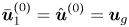 $\bar {\boldsymbol {u}}_1^{(0)} = \hat {\boldsymbol {u}}^{(0)} = \boldsymbol {u}_{g}$, and
 $C_{5}=\bar {c}^{(0)}$.
At the next order of (3.2)–(3.4),  $\mathcal {O}(\epsilon ^{-1})$, we obtain
 \begin{align} (\phi\boldsymbol{n}\boldsymbol{\cdot} \hat{\boldsymbol{u}}^{(0)})_z - \boldsymbol{u}_{g}\boldsymbol{\cdot}\boldsymbol{n}\phi_z =0&= \alpha\left(M(\hat{c}^{(0)})\phi (\hat{\mu}^{(1)}+\alpha\hat{p}^{(1)})_z\right)_z\nonumber\\ &\quad +\alpha\left(M(\hat{c}^{(1)})\phi (\hat{\mu}^{(0)}+\alpha\hat{p}^{(0)})_z\right)_z, \end{align}
 \begin{gather} \left(\phi M(\hat{c}^{(0)})(\hat{\mu}^{(1)}+\alpha \hat{p}^{(1)})_z\right)_z = -\hat{\boldsymbol{u}}^{(0)}\boldsymbol{\cdot} \boldsymbol{n}(\phi\hat{c}^{(0)})_z + \hat{\boldsymbol{u}}^{(0)}\boldsymbol{\cdot} \boldsymbol{n}(\phi \hat{c}^{(0)})_z = 0, \end{gather}
 \begin{gather}(\phi\hat{c}_z^{(1)})_z = -\frac{\phi_z}{\epsilon_c\sqrt{2}}\cos(\theta))\left(1-\bar{c}^{(0)}\right) \bar{c}^{(0)}. \end{gather}
Integrating (A 28) and (A 29) both sides from  $-\infty$ to
 $+\infty$ with respect to
 $z$, we have
 \begin{gather} \lim_{z\rightarrow-\infty}(\hat{\mu}^{(1)}+\alpha\hat{p}^{(1)})_z=0, \end{gather}
 \begin{gather}\lim_{z\rightarrow-\infty}\hat{c}_z^{(1)} = \frac{1}{\epsilon_c\sqrt{2}}\cos(\theta)\left(1-\bar{c}^{(0)}\right)\bar{c}^{(0)}. \end{gather}
Using the matching condition (A 15), we obtain
 \begin{gather} \boldsymbol{n}\boldsymbol{\cdot}\boldsymbol{\nabla} (\bar{\mu}_1^{(0)}+\alpha\bar{p}_1^{(0)})=0, \end{gather}
 \begin{gather}\boldsymbol{n}\boldsymbol{\cdot}\boldsymbol{\nabla} \bar{c}_1^{(0)} = \frac{1}{\epsilon_c\sqrt{2}}\cos(\theta)\left(1-\bar{c}^{(0)}\right)\bar{c}^{(0)}. \end{gather}
Therefore, the outer solutions  $\bar {\boldsymbol {u}}_1^{(0)}$,
 $\bar {\mu }_1^{(0)}$,
 $\bar {p}_1^{(0)}$ and
 $\bar {c}_1^{(0)}$ satisfy the original boundary conditions (2.38)–(2.40). Hence the q-NSCH-DD system recovers the q-NSCH model at leading order.
Appendix B. Numerical method and implementation
We now present a projection method for the q-NSCH-DD system (3.1)–(3.4) at the time-discrete level. Let  $\textrm {d} t>0$ denote the time step, and assume
 $\boldsymbol {u}^{n}$,
 $p^{n}$,
 $c^{n}$ and
 $\mu ^{n}$ are the solutions at time
 $t=n\,\textrm {d}t$. The solutions at time
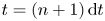 $t= (n+1)\,\textrm {d} t$, namely
 $\boldsymbol {u}^{n+1}$,
 $p^{n+1}$,
 $c^{n+1}$ and
 $\mu ^{n+1}$, are given by
 \begin{align} \frac{\phi^{n+1}c^{n+1}-\phi^{n}c^{n}}{\textrm{d} t}+\boldsymbol{\nabla} \boldsymbol{\cdot} \left(\phi^{n} \boldsymbol{u}^{n}c^{n}\right)&= \boldsymbol{\nabla}\boldsymbol{\cdot}\left(\phi^{n+1} M(c^{n+1}) \boldsymbol{\nabla} \mu^{n+1}\right)\nonumber\\ &\quad +\alpha\boldsymbol{\nabla}\boldsymbol{\cdot}\left(\phi^{n+1} M(c^{n+1}) \boldsymbol{\nabla} p^{n}\right), \end{align}
 \begin{align} \phi^{n+1} \mu^{n+1}&= \phi^{n+1} \epsilon_c F'(c^{n+1})-\epsilon_c^2 \boldsymbol{\nabla} \boldsymbol{\cdot}(\phi^{n+1} \boldsymbol{\nabla}c^{n+1})\nonumber\\ &\quad -\frac{\epsilon_c|\boldsymbol{\nabla} \phi^{n+1}|}{\sqrt{2}}\cos(\theta)\left(1-c^{n+1}\right)c^{n+1}, \end{align}
 \begin{align} &\frac{\phi^{n+1}\rho^{n+1}\boldsymbol{\tilde{u}}^{n+1}-\phi^n\rho^{n}\boldsymbol{u}^{n}}{\textrm{d}t} + \rho^{n}\boldsymbol{u}^n \boldsymbol{\cdot}\boldsymbol{\boldsymbol{\nabla}}(\phi^n\boldsymbol{u}^n)\nonumber\\ &\quad =\phi^{n+1}{\boldsymbol{\nabla}}\boldsymbol{\cdot}\left(\nu^{n}{\boldsymbol\nabla} \boldsymbol{ \tilde{u}}^{n+1}\right)+ \frac{\tilde{\sigma}}{\epsilon_c}\mu^{n+1}\boldsymbol{\nabla} c^{n+1} \nonumber\\ &\qquad +\frac{1}{3}\phi^{n+1}\boldsymbol{\nabla}\left(\nu^{n}{\boldsymbol\nabla} \boldsymbol{\cdot} \boldsymbol{\tilde{u}}^{n+1}\right)- \frac{\left(1-\phi^{n+1}\right)}{\epsilon^2} \left(\boldsymbol{\tilde{u}}^{n+1}-\boldsymbol{u}_{g}^{n+1}\right)- \phi^{n+1}\rho^{n+1} g\boldsymbol{z}, \end{align}
 \begin{align} \textrm{d}t{\boldsymbol\nabla} \boldsymbol{\cdot} \left(\frac{\phi^{n+1}}{\rho^{n+1}} {\boldsymbol\nabla} p^{n+1}\right)&={\boldsymbol\nabla} \boldsymbol{\cdot} \left(\phi^{n+1} \boldsymbol{\tilde{u}}^{n+1}\right)-\boldsymbol{u}_{g}^{n+1}\boldsymbol{\cdot} {\boldsymbol{\nabla}} \phi^{n+1} \nonumber\\ &\quad +\alpha\boldsymbol{\nabla}\boldsymbol{\cdot}\left(\phi^{n+1} M(c^{n+1}) \boldsymbol{\nabla} \mu^{n+1}\right)+\alpha^2\boldsymbol{\nabla}\boldsymbol{\cdot}\left(\phi^{n+1} M(c^{n+1}) \boldsymbol{\nabla} p^{n+1}\right)\nonumber\\ &\quad -\textrm{d}t{\boldsymbol\nabla}\boldsymbol{\cdot} \frac{\left(1-\phi^{n+1}\right)}{\epsilon^2\rho^{n+1}}\left(\boldsymbol{u}^{n+1}- \boldsymbol{\tilde{u}}^{n+1}\right), \end{align}
 \begin{equation} \boldsymbol{u}^{n+1}=\boldsymbol{\tilde{u}}^{n+1}-\dfrac{\phi^{n+1}{\boldsymbol\nabla} p^{n+1}}{\dfrac{\phi^{n+1}\rho^{n+1}}{\textrm{d}t}+\dfrac{(1-\phi^{n+1})}{\epsilon^2}}, \end{equation}
with the following boundary conditions:
 \begin{equation} \tilde{\boldsymbol{u}}^{n+1}|_{\partial \tilde{\varOmega}}=\boldsymbol{u}^{n+1}|_{\partial \tilde{\varOmega}}=0,\quad\boldsymbol{n} \boldsymbol{\cdot}\boldsymbol{\nabla}c^{n+1}|_{\partial \tilde{\varOmega}}=\boldsymbol{n} \boldsymbol{\cdot}\boldsymbol{\nabla} (\mu^{n+1}+\alpha p^{n+1})|_{\partial \tilde{\varOmega}}=0. \end{equation}
Here we introduce a temporary velocity,  $\tilde {\boldsymbol {u}}$, to split the original momentum (3.1). We first solve (B 1) and (B 2) to get
 $c^{n+1}$ and
 $\mu ^{n+1}$ , we then obtain
 $\tilde {\boldsymbol {u}}^{n+1}$ and
 $p^{n+1}$ from (B 3) and (B 4). Finally the velocity
 $\boldsymbol {u}^{n+1}$ is updated in (B 5).
At the fully discrete level, our method uses a finite difference method on a staggered grid and implemented using an efficient, practical nonlinear multigrid solver, which was originally developed for solving a diffuse interface model for two-phase flows (Guo et al. Reference Guo, Lin, Lowengrub and Wise2017). In particular, we save the vector field, the velocity  $\boldsymbol {u}=(u,v)$, as the edge-centred variables, and all the scalar variables
 $c$,
 $\mu$,
 $\phi$ and
 $p$ as the cell-centred variables. Here we use a regularized
 $\tilde {\phi }=\phi +\delta$, where
 $\delta =10^{-6}$. The scheme is comprised of a standard FAS method for the Cahn–Hilliard equations (B 1) and (B 2), and a method based on the Vanka-type smoothing strategy for the Navier–Stokes equations (B 3)–(B 5). As demonstrated in Guo et al. (Reference Guo, Lin, Lowengrub and Wise2017), the numerical method is first-order accurate in time and second-order accurate in space.