2 Problem formulation

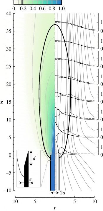
As indicated in figure 1, the configuration analysed includes a vertical fuel jet discharging upwards through an injector of inner radius $a$ into an infinite air atmosphere. The specific geometry investigated here involves a thin injector of thickness $e\ll a$ . To minimize wake effects, the rim of the injector is knife-like sharpened as indicated in the inset of figure 1. For the numerical integrations shown below, the injector wall thickness and the slenderness ratio of the wedge tip were selected to be $e/a=10^{-3}$ and $d/e=20$ , respectively. Smaller values of $e/a$ and larger values of $d/e$ were used in sample integrations to ensure that the results were independent of these two geometric parameters, so that the solution given below is representative of infinitesimally thin injectors.

Figure 1.

Base flow isocontours of  $\bar{Z}$ (left-hand side) and streamlines (right-hand side) together with radial profiles of  $\bar{v}_{x}$ (solid curves) and  $\bar{T}/({\it\gamma}+1)$ (dashed curves) at $x=(0,5,10,15,20,25,30,35)$ for $\mathit{Pr}=0.7$ , $S=4.62$ , ${\it\gamma}=6$ , $\mathit{Re}=100$ and $\mathit{Fr}=300$ . The dot on the velocity profiles indicates the location of the inflection points. The thick solid line represents the stoichiometric flame surface $\bar{Z}=Z_{S}$ , where $\bar{T}=1+{\it\gamma}$ .

For generality, the analysis considers dilution of the fuel with an inert gas, with $Y_{F,0}$ denoting the fuel mass fraction in its feed stream, while $Y_{\text{O}_{2},A}=0.232$ is the oxygen mass fraction in air. In the description, focused on the fluid mechanical aspects of the flow, we adopt the one-step irreversible overall reaction $F+s\,\text{O}_{2}\rightarrow (1+s)\,\text{Products}+q$ , according to which the unit mass of fuel reacts with a mass $s$ of oxygen, releasing in the process an amount of energy $q$ . The above representation of the underlying stoichiometry for the oxidation of the fuel embodies the two fundamental thermochemical parameters involved in non-premixed combustion (Liñán et al. Reference Liñán, Vera and Sánchez2015),

(2.1a,b ) $$\begin{eqnarray}S=\frac{sY_{F,0}}{Y_{\text{O}_{2},A}}\quad \text{and}\quad {\it\gamma}=\frac{qY_{F,0}}{c_{p}T_{0}^{\prime }(1+S)},\end{eqnarray}$$

the former representing the mass of air that one needs to mix with the unit mass of the gaseous fuel stream to generate a stoichiometric mixture and the latter being the corresponding dimensionless temperature increment resulting from the adiabatic combustion of that mixture. Here, $T_{0}^{\prime }$ is the initial temperature of the feed streams, assumed to be equal for the fuel jet and for the surrounding air atmosphere, and $c_{p}$ represents the specific heat at constant pressure, taken to be constant in the following analysis. Typical values for undiluted hydrocarbon–air flames initially at normal ambient temperature are $S_{u}=s/Y_{\text{O}_{2},A}\simeq 15$ and ${\it\gamma}_{u}\simeq 6{-}7$ . Diluting the fuel stream with an inert gas to give a fuel mass fraction $Y_{F,0}<1$ in its feed stream has a direct effect on the value of $S=Y_{F,0}S_{u}$ , but a much more limited effect on the heat-release parameter, as can be seen by writing the second expression in (2.1) for $S_{u}\gg 1$ in the approximate form $({\it\gamma}_{u}-{\it\gamma})/{\it\gamma}_{u}\simeq (1+Y_{F,0}S_{u})^{-1}$ , which indicates that significant variations of ${\it\gamma}$ require extremely dilute fuel mixtures such that $Y_{F,0}\sim S_{u}^{-1}$ .

In the limit of infinitely fast reaction adopted here, the reaction takes place in an infinitesimally thin layer, outside of which the chemical equilibrium condition ${\hat{Y}}_{F}{\hat{Y}}_{\text{O}}=0$ applies, with ${\hat{Y}}_{F}=Y_{F}/Y_{F,0}$ and ${\hat{Y}}_{\text{O}}=Y_{\text{O}_{2}}/Y_{\text{O}_{2},A}$ representing the fuel and oxygen mass fractions normalized with their values in their respective feed streams. The reaction-rate terms in the conservation equations for energy and species appear as Dirac delta distributions located at the flame, which latter becomes in this limit an infinitesimally thin surface attached to the injector separating a near-axis region without oxygen from a fuel-free outer atmosphere (Burke & Schumann Reference Burke and Schumann1928). For equidiffusive reactants, Shvab (Reference Shvab and Knorre1948) and Zel’dovich (Reference Zel’dovich1949) showed how the computation can be facilitated by the introduction of conserved scalars satisfying transport equations, obtained by combinations of the species and energy conservation equations that eliminate the chemical source terms. Two conveniently normalized forms of these passive scalars are the mixture fraction and the excess enthalpy, defined as

(2.2a,b ) $$\begin{eqnarray}Z=\frac{S{\hat{Y}}_{F}-{\hat{Y}}_{\text{O}}+1}{S+1}\quad \text{and}\quad H=T-1+{\it\gamma}({\hat{Y}}_{F}+{\hat{Y}}_{\text{O}}-1),\end{eqnarray}$$

where the non-dimensional temperature $T$ has been scaled with $T_{0}^{\prime }$ . The mixture fraction is defined to be zero in the air stream and unity in the fuel stream, respectively, whereas at the flame, where both reactants appear in zero concentrations, $Z$ takes the stoichiometric value $Z_{S}=1/(S+1)$ . On the other hand, the excess enthalpy is defined to be zero in both feed streams, so that when the injector walls are adiabatic, which is the case considered here, the solution for the associated transport equation reduces to $H=0$ everywhere in the flow field, thereby facilitating the description. The piecewise-linear expressions

(2.3a-c ) $$\begin{eqnarray}\displaystyle & \displaystyle {\hat{Y}}_{F}=0,\quad {\hat{Y}}_{\text{O}}=1-\frac{Z}{Z_{S}},\quad T-1={\it\gamma}\frac{Z}{Z_{S}},\quad \text{for}\;0\leqslant Z\leqslant Z_{S}, & \displaystyle\end{eqnarray}$$

(2.3d-f ) $$\begin{eqnarray}\displaystyle & \displaystyle {\hat{Y}}_{\text{O}}=0,\quad {\hat{Y}}_{F}=\frac{Z-Z_{S}}{1-Z_{S}},\quad T-1={\it\gamma}\frac{1-Z}{1-Z_{S}},\quad \text{for}\;Z_{S}\leqslant Z\leqslant 1, & \displaystyle\end{eqnarray}$$

obtained from the definitions (2.2) with use made of the equilibrium condition ${\hat{Y}}_{F}{\hat{Y}}_{\text{O}}=0$ and of the result $H=0$ , provide the reactant mass fractions and temperature in terms of $Z$ . Evaluation of the expressions for $T$ at $Z=Z_{S}$ indicates that the temperature at the flame surface is everywhere equal to the stoichiometric adiabatic flame temperature $T=1+{\it\gamma}$ , a known result of the infinitely fast reaction limit that holds in adiabatic configurations with unity Lewis numbers of the reactants.

The problem reduces to that of integrating the continuity and momentum equations together with the transport equation for $Z$ , which are written in the dimensionless form

(2.4) $$\begin{eqnarray}\displaystyle & \displaystyle \frac{\partial {\it\rho}}{\partial t}+\boldsymbol{{\rm\nabla}}\boldsymbol{\cdot }{\it\rho}\boldsymbol{v}=0, & \displaystyle\end{eqnarray}$$

(2.5) $$\begin{eqnarray}\displaystyle & \displaystyle {\it\rho}\frac{\partial \boldsymbol{v}}{\partial t}+{\it\rho}\boldsymbol{v}\boldsymbol{\cdot }\boldsymbol{{\rm\nabla}}\boldsymbol{v}=-\boldsymbol{{\rm\nabla}}p+\frac{1}{\mathit{Re}}\boldsymbol{{\rm\nabla}}\boldsymbol{\cdot }\bar{\bar{{\it\tau}}}+\frac{1}{\mathit{Fr}}(1-{\it\rho})\boldsymbol{e}_{x}, & \displaystyle\end{eqnarray}$$

(2.6) $$\begin{eqnarray}\displaystyle & \displaystyle {\it\rho}\frac{\partial Z}{\partial t}+{\it\rho}\boldsymbol{v}\boldsymbol{\cdot }\boldsymbol{{\rm\nabla}}Z=\frac{1}{\mathit{Re}\,\mathit{Pr}}\boldsymbol{{\rm\nabla}}\boldsymbol{\cdot }({\it\rho}D_{T}\boldsymbol{{\rm\nabla}}Z), & \displaystyle\end{eqnarray}$$

where $\mathit{Pr}=0.7$ is the Prandtl number and

(2.7a,b ) $$\begin{eqnarray}\mathit{Re}=\frac{{\it\rho}_{0}^{\prime }U_{0}a}{{\it\mu}_{0}^{\prime }}\quad \text{and}\quad \mathit{Fr}=\frac{U_{0}^{2}}{ga}\end{eqnarray}$$

are the Reynolds number and the Froude number for the jet flow, respectively, with ${\it\rho}_{0}^{\prime }$ and ${\it\mu}_{0}^{\prime }$ representing the density and shear viscosity in the feed streams. The jet radius $a$ and the average jet velocity $U_{0}={\dot{m}}/({\rm\pi}a^{2}{\it\rho}_{0}^{\prime })$ based on the fuel mass flow rate ${\dot{m}}$ are used to scale the problem. The development employs axisymmetric cylindrical coordinates $\boldsymbol{x}=(x,r)$ centred at the injector exit plane with an associated velocity vector $\boldsymbol{v}=(v_{x},v_{r})$ ; the streamwise coordinate $x$ pointing against the gravity vector $\boldsymbol{g}=-g\boldsymbol{e}_{x}$ .

In the low Mach number approximation utilized here, the pressure variations can be neglected in the first approximation when writing the equation of state, which therefore reduces to ${\it\rho}T=1$ when the additional assumption of constant molecular weight is adopted to achieve maximum simplification, with ${\it\rho}={\it\rho}^{\prime }/{\it\rho}_{0}^{\prime }$ denoting the dimensionless density. Furthermore, in this low Mach number limit, the viscous stress term proportional to the second viscosity coefficient can be incorporated in the definition of the variable $p$ that represents in (2.5) the pressure difference from the unperturbed ambient distribution. Correspondingly, the resulting viscous stress tensor reduces to $\bar{\bar{{\it\tau}}}={\it\mu}(\boldsymbol{{\rm\nabla}}\boldsymbol{v}+\boldsymbol{{\rm\nabla}}\boldsymbol{v}^{\text{T}})$ , with both $p$ and $\bar{\bar{{\it\tau}}}$ scaled with the characteristic value of the dynamic pressure ${\it\rho}_{0}^{\prime }U_{0}^{2}$ . The power-law expressions ${\it\mu}={\it\rho}D_{T}=T^{{\it\sigma}}$ , with ${\it\sigma}=0.7$ , are employed for the temperature dependence of the shear viscosity ${\it\mu}$ and thermal diffusivity $D_{T}$ , both scaled with their feed-stream values.

Equations (2.4)–(2.6) must be integrated with appropriate conditions on the boundaries of the computational domain, which includes an outer cylindrical boundary with radius $r_{\mathit{max}}\gg 1$ , with downstream and upstream boundaries located at $x=x_{d}$ and at $x=x_{u}$ . The results corresponding to the most unstable mode were tested to be independent of the size of the computational domain, with the values $r_{\mathit{max}}=45$ , $x_{d}=450$ and $x_{u}=-10$ selected for the computations shown below. The injector is assumed to be sufficiently long for the fuel flow to be fully developed, thereby giving $\boldsymbol{v}=2\,(1-r^{2})\boldsymbol{e}_{x}$ and $Z=1$ in the fuel boundary upstream from the injector exit (i.e. at $x=x_{u}$ for $0\leqslant r\leqslant 1$ ). On the injector walls the solution satisfies the non-slip condition $\boldsymbol{v}=0$ , together with the condition $\boldsymbol{n}\boldsymbol{\cdot }\boldsymbol{{\rm\nabla}}Z=0$ corresponding to an impermeable wall, with $\boldsymbol{n}$ representing here the normal unit vector. To let the air enter or leave the computational domain as required to satisfy the development and the entrainment needs of the jet, a stress-free condition $-p\boldsymbol{n}+\bar{\bar{{\it\tau}}}\boldsymbol{\cdot }\boldsymbol{n}/\mathit{Re}=0$ is applied all around the outer air boundary. Air enters the flow field through the lateral boundary and through the upstream boundary, so that the condition $Z=0$ applies there, whereas $\boldsymbol{n}\boldsymbol{\cdot }\boldsymbol{{\rm\nabla}}Z=0$ must be used on the downstream boundary to allow for the evacuation of the combustion products.

3 The global linear stability analysis

3.1 The eigenvalue problem

Introduction of the temporal normal mode decomposition $(\boldsymbol{v},p,Z)=(\bar{\boldsymbol{v}},\bar{p},\bar{Z})+{\it\varepsilon}(\hat{\boldsymbol{v}},\hat{p},\hat{Z})\text{e}^{-\text{i}{\it\omega}t}$ , involving the steady base flow $(\bar{\boldsymbol{v}},\bar{p},\bar{Z})(\boldsymbol{x})$ , the eigenfunctions $(\hat{\boldsymbol{v}},\hat{p},\hat{Z})(\boldsymbol{x})$ multiplied by an arbitrarily small factor ${\it\varepsilon}$ , and the complex angular frequency ${\it\omega}={\it\omega}_{r}+\text{i}{\it\omega}_{i}$ , leads to a set of nonlinear equations for the base flow (i.e. the steady counterpart of (2.4)–(2.6)), to be integrated with the boundary conditions stated in the last paragraph of the preceding section. The associated linear equations for the perturbed flow

(3.1) $$\begin{eqnarray}\displaystyle & \displaystyle -\text{i}{\it\omega}\hat{{\it\rho}}+\boldsymbol{{\rm\nabla}}\boldsymbol{\cdot }\hat{{\it\rho}}\bar{\boldsymbol{v}}+\boldsymbol{{\rm\nabla}}\boldsymbol{\cdot }\bar{{\it\rho}}\hat{\boldsymbol{v}}=0, & \displaystyle\end{eqnarray}$$

(3.2) $$\begin{eqnarray}\displaystyle & & \displaystyle -\text{i}{\it\omega}\bar{{\it\rho}}\hat{\boldsymbol{v}}+\hat{{\it\rho}}\bar{\boldsymbol{v}}\boldsymbol{\cdot }\boldsymbol{{\rm\nabla}}\bar{\boldsymbol{v}}+\bar{{\it\rho}}\hat{\boldsymbol{v}}\boldsymbol{\cdot }\boldsymbol{{\rm\nabla}}\bar{\boldsymbol{v}}+\bar{{\it\rho}}\bar{\boldsymbol{v}}\boldsymbol{\cdot }\boldsymbol{{\rm\nabla}}\hat{\boldsymbol{v}}\nonumber\\ \displaystyle & & \displaystyle \quad =-\boldsymbol{{\rm\nabla}}\hat{p}-\frac{1}{\mathit{Fr}}\hat{{\it\rho}}\boldsymbol{e}_{x}+\frac{1}{\mathit{Re}}\boldsymbol{{\rm\nabla}}\boldsymbol{\cdot }[\hat{{\it\mu}}(\boldsymbol{{\rm\nabla}}\bar{\boldsymbol{v}}+\boldsymbol{{\rm\nabla}}\bar{\boldsymbol{v}}^{\text{T}})+\bar{T}^{{\it\sigma}}(\boldsymbol{{\rm\nabla}}\hat{\boldsymbol{v}}+\boldsymbol{{\rm\nabla}}\hat{\boldsymbol{v}}^{\text{T}})],\end{eqnarray}$$

(3.3) $$\begin{eqnarray}\displaystyle & \displaystyle -\text{i}{\it\omega}\bar{{\it\rho}}\hat{Z}+\hat{{\it\rho}}\bar{\boldsymbol{v}}\boldsymbol{\cdot }\boldsymbol{{\rm\nabla}}\bar{Z}+\bar{{\it\rho}}\hat{\boldsymbol{v}}\boldsymbol{\cdot }\boldsymbol{{\rm\nabla}}\bar{Z}+\bar{{\it\rho}}\bar{\boldsymbol{v}}\boldsymbol{\cdot }\boldsymbol{{\rm\nabla}}\hat{Z}=\frac{1}{\mathit{Re}\,\mathit{Pr}}\boldsymbol{{\rm\nabla}}\boldsymbol{\cdot }[(\hat{{\it\mu}}\boldsymbol{{\rm\nabla}}\bar{Z}+\bar{T}^{{\it\sigma}}\boldsymbol{{\rm\nabla}}\hat{Z})], & \displaystyle\end{eqnarray}$$

arise from linearization of (2.4)–(2.6); these must be supplemented with $\hat{{\it\rho}}/\bar{{\it\rho}}=-\hat{T}/\bar{T}$ and $\hat{{\it\mu}}={\it\sigma}\bar{T}^{{\it\sigma}-1}\hat{T}$ , which follow from the equation of state and from the transport description, and with $\hat{T}={\it\gamma}\hat{Z}/Z_{S}$ for $0\leqslant \bar{Z}\leqslant Z_{S}$ and $\hat{T}=-{\it\gamma}\hat{Z}/(1-Z_{S})$ for $Z_{S}\leqslant \bar{Z}\leqslant 1$ , which follow from (2.3). Boundary conditions for (3.2)–(3.3) are $\hat{\boldsymbol{v}}=\hat{Z}=0$ in the fuel stream and $\hat{\boldsymbol{v}}=\boldsymbol{n}\boldsymbol{\cdot }\boldsymbol{{\rm\nabla}}\hat{Z}=0$ on the injector wall. On the air boundary, the stress-free condition for the perturbed flow reduces to $-\hat{p}\boldsymbol{n}+(\boldsymbol{{\rm\nabla}}\hat{\boldsymbol{v}}+\boldsymbol{{\rm\nabla}}\hat{\boldsymbol{v}}^{\text{T}})\boldsymbol{\cdot }\boldsymbol{n}/\mathit{Re}=0$ on the upstream and lateral air boundaries, where $\hat{Z}=0$ , and to ${\it\sigma}{\it\gamma}\,[(\bar{p}/\bar{T})(\hat{Z}/Z_{S})-\hat{p}]\,\boldsymbol{n}+\bar{T}^{{\it\sigma}}(\boldsymbol{{\rm\nabla}}\hat{\boldsymbol{v}}+\boldsymbol{{\rm\nabla}}\hat{\boldsymbol{v}}^{\text{T}})\boldsymbol{\cdot }\boldsymbol{n}/\mathit{Re}=0$ on the downstream boundary, where $\boldsymbol{n}\boldsymbol{\cdot }\boldsymbol{{\rm\nabla}}\hat{Z}=0$ . Non-trivial solutions $(\hat{\boldsymbol{v}},\hat{p},\hat{Z})\neq 0$ are found for a discrete set of eigenvalues ${\it\omega}$ . The real part of ${\it\omega}$ is the frequency of the perturbation, defining a Strouhal number $\mathit{St}={\it\omega}_{r}/{\rm\pi}$ (the ratio of the residence time $2a/U_{0}$ to the period of the oscillation); the imaginary part is the growth rate, which dictates whether the flame is globally stable ( ${\it\omega}_{i}<0$ ) or unstable ( ${\it\omega}_{i}>0$ ).

3.2 Sample numerical results

The base flow was integrated using a finite-element method with $P1$ elements for the pressure field and $P2$ elements for the remaining variables, combined with a Newton–Raphson root-finding algorithm; details of the discretization method, used for instance by Garnaud et al. (Reference Garnaud, Lesshafft, Schmid and Huerre2013b ), can be found in Hecht (Reference Hecht2012). The same finite-element formalism was employed to discretize the perturbed equations, resulting in a generalized eigenvalue problem that was solved using a shifted inverse power method (Lehoucq, Sorensen & Yang Reference Lehoucq, Sorensen and Yang1998).

The integrations explored in particular configurations with $2.08\leqslant S\leqslant 9.66$ and moderately large values of $\mathit{Re}$ , for which the resulting flame height is much larger than the injector radius, as shown in figure 1 for the case $S=4.62$ , $\mathit{Re}=100$ and $\mathit{Fr}=300$ . A thick solid curve is used to denote the flame location, where $\bar{Z}=Z_{S}\simeq 0.178$ and $\bar{T}/({\it\gamma}+1)=1$ . Besides isocontours of $\bar{Z}$ , the plot includes streamlines, which serve to illustrate the motion of the air induced by the entrainment of the mixing layer surrounding the flame envelope.

Radial profiles of axial velocity $\bar{v}_{x}$ and normalized temperature $\bar{T}/({\it\gamma}+1)$ are represented in figure 1 at different axial locations. Even for this relatively large Froude number, buoyancy is seen to accelerate the flow in the flame envelope, leading to the appearance of two inflection points in the velocity profile near the flame, additional to the inflection point associated with the shape of the initial velocity profile (the locations of these inflection points are marked with a dot). As shown previously for mixing layers (Soteriou & Ghoniem Reference Soteriou and Ghoniem1995) and low-density jets (Lesshafft & Huerre Reference Lesshafft and Huerre2007), the action of the baroclinic torque, induced in jet flames by the radial density gradient present in the near-flame region where the velocity profile displays inflection points, plays a key role in the development of a region of absolute stability (Lingens et al. Reference Lingens, Neemann, Meyer and Schreiber1996a ), which in turn triggers the global oscillations. The rate at which the induced perturbations are convected away from this wavemaker region depends on the local value of the axial velocity, with smaller velocities favouring the development of absolute instabilities (Lesshafft & Marquet Reference Lesshafft and Marquet2010).

Figure 2.

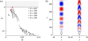
(a) Eigenvalue spectra for $\mathit{Pr}=0.7$ , $S=4.62$ , ${\it\gamma}=6$ , $\mathit{Re}=100$ and $\mathit{Fr}=(250,300,400,550,625)$ . (b) Real part of the streamwise velocity $\hat{v}_{x}$ (left) and mixture fraction $\hat{Z}$ (right) for the eigenfunctions of the most unstable mode with $\mathit{Re}=100$ and $\mathit{Fr}=300$ .

Figure 2(a) shows the eigenvalue spectra computed for $\mathit{Re}=100$ and different values of $\mathit{Fr}$ . For all cases, the most unstable eigenmode is indicated with a bigger symbol in red. Decreasing the Froude number is seen to destabilize the flow, so that for $\mathit{Fr}=300$ the growth rate ${\it\omega}_{i}$ of the most unstable mode is still negative, but it is already positive for $\mathit{Fr}=250$ . For completeness, eigenmodes corresponding to the subcritical case $\mathit{Fr}=300$ are plotted in figure 2(b). As can be seen, both the radial extent of the eigenmodes and their wavelength scale with the flame dimensions. Although the length $x_{d}=450$ of the computational domain was not long enough to capture the downstream decay of the eigenmodes, the associated values of ${\it\omega}$ for the most unstable mode were seen to be independent of $x_{d}$ provided that $x_{d}>400$ , as verified in a series of computations.

3.3 Transition diagrams

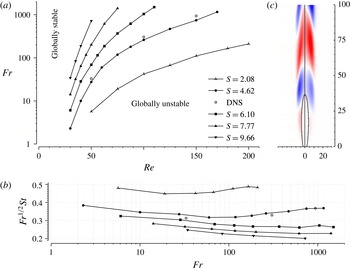
Marginal conditions were determined by linear interpolation of the results of stability spectra computed for given values of $S$ and $\mathit{Re}$ and decreasing values of $\mathit{Fr}$ (including stable and unstable cases), giving the transition diagrams and accompanying frequencies shown in figure 3. The resulting marginal curves serve to assess effects of fuel-feed dilution and of molecular transport. Increasing $\mathit{Re}$ for a given value of $S$ is seen to have a destabilizing effect, in that the global instability sets in at a higher value of $\mathit{Fr}$ , in agreement with recent observations for low-density jets (Coenen et al. Reference Coenen, Lesshafft, Garnaud and Sevilla2016). Conversely, fuel-feed dilution (i.e. decreasing values of  $S$ ) tends to stabilize the flow, a result that can be explained by noticing that dilute flames sit closer to the axis, where the downstream convective rate of the perturbations is higher, thereby hindering the development of a region of absolute instability and resulting in smaller critical values of $\mathit{Fr}$ .

Figure 3.

(a) Transition diagram in the $\mathit{Re}{-}\mathit{Fr}$ parametric plane for different values of $S$ , with the (b) accompanying panel showing the variation with $\mathit{Fr}$ of the non-dimensional frequency $\mathit{Fr}^{1/2}\mathit{St}=({\it\omega}_{r}/{\rm\pi})/\sqrt{g/a}$ at the margin of instability and the empty symbols in both plots representing DNS predictions for $\mathit{Re}=(50,100,150)$ . As explained in the text, (c) a comparison for $S=4.62$ , $\mathit{Re}=100$ and $\mathit{Fr}=261.40$ of the eigenmode $\hat{T}(\boldsymbol{x})$ (right-hand side) with a snapshot extracted from the DNS results (left-hand side).

The large variations in critical values of $\mathit{Fr}$ observed in figure 3(a) would be considerably reduced should the characteristic scales of the flame, rather than those associated with fuel injection, be used in defining the relevant Froude number (Liñán et al. Reference Liñán, Vera and Sánchez2015). Thus, with $\mathit{Re}\gg 1$ and $S\gg 1$ the flame length is of the order of $S\,\mathit{Re}\,a$ . At these distances, the jet velocity has decreased to values of the order of $U_{0}/S$ , which must be compared with the buoyancy-induced velocity $g\,S\,\mathit{Re}\,a$ , the square of their ratio giving $\mathit{Fr}/(S^{3}\mathit{Re})$ as the relevant Froude number for jet flames. Inspection of the results in figure 3(a) reveals that this alternative definition would result in a transition diagram with less pronounced variations of the critical Froude number over the range of conditions explored.

For the range of Reynolds numbers explored in figure 3, the effective Froude number accounting for the residence time in the flame region $\mathit{Fr}/(S^{3}\mathit{Re})$ is somewhat smaller than unity, corresponding to jet flames with significant buoyancy effects. Consequently, the dynamics of the resulting oscillations at the margin of stability is characterized by the buoyancy time $\sqrt{a/g}$ , rather than by the residence time $a/U_{0}$ employed initially in non-dimensionalizing the problem. This scaling is tested in figure 3(b), where the frequency is represented in terms of $({\it\omega}_{r}/{\rm\pi})/\sqrt{g/a}=\mathit{Fr}^{1/2}\mathit{St}$ . As can be seen, for each value of $S$ , the resulting frequencies change only by approximately 10 % over the whole range of Froude numbers explored in the figure, thereby demonstrating the prevalence of the buoyancy scaling. This is in agreement with the experimental observations of Durox & Villermaux (Reference Durox, Yuan and Villermaux1997) and Sato, Amagai & Arai (Reference Sato, Amagai and Arai2000), who found that $\mathit{St}\sim \mathit{Fr}^{-1/2}$ .

The buoyancy-dominated flickering mode observed here is markedly different from that corresponding to buoyancy-free light jets and flames, for which the resulting frequencies scale with $a/U_{0}$ , with associated eigenmodes scaling with the jet radius rather than with the flame length. This alternative buoyancy-free mode, which must become dominant at sufficiently high Froude numbers (and sufficiently high accompanying Reynolds numbers), was not observed in the computations carried out here. For the Poiseuille exit velocity profile considered in our work, preliminary computations for $\mathit{Fr}=\infty$ and $S=6.10$ indicated that non-buoyant flames are globally stable up to the largest Reynolds number considered ( $\mathit{Re}=1000$ ). A critical Reynolds number exceeding 1000 for buoyancy-free jet flames is consistent with previous results concerning the influence of the exit velocity profile on the stability of light jets (Hallberg & Strykowski Reference Hallberg and Strykowski2006). Smaller critical values of the Reynolds number are expected, for instance, for nearly uniform profiles, encountered with shorter fuel injectors.

4 Comparison with DNS results

The predictions of the stability analysis at the margin of stability were compared with DNS results obtained with a time-dependent axisymmetric code (Carpio, Prieto & Vera Reference Carpio, Prieto and Vera2016) using the same grid employed in the global stability computations. The numerical simulations at three different points along the marginal curve for $S=4.62$ , namely, $(\mathit{Re},\mathit{Fr})=(50,26.60)$ , $(\mathit{Re},\mathit{Fr})=(100,261.40)$ and $(\mathit{Re},\mathit{Fr})=(150,745.64)$ , yielded periodic solutions with small amplitude. The associated Strouhal numbers, $\mathit{St}=(0.0628,0.0200,0.0132)$ , obtained by fitting the oscillations of the numerical solutions to a sinusoidal function, were seen to be in excellent agreement with the values $\mathit{St}=(0.0638,0.0190,0.0134)$ predicted by the stability analysis. The agreement extends to the morphology of the flickering mode, as can be seen in figure 3(c), which compares the eigenmode $\hat{T}(\boldsymbol{x})$ corresponding to $(\mathit{Re},\mathit{Fr})=(100,261.40)$ with the near-critical DNS results, the latter obtained by subtracting the time-averaged temperature from the instantaneous distribution $T(\boldsymbol{x};t^{\ast })$ , with the time $t^{\ast }$ appropriately selected to minimize the observed differences. As can be seen, there exists excellent agreement not only in the predicted wavelength, but also in the shape of the cells representing the travelling rollers.

As mentioned above, for the parametric values corresponding to the marginal conditions of the stability analysis, the DNS results were seen to exhibit small oscillations of non-negligible amplitude. Additional computations for increasing values of $\mathit{Fr}$ , resulting in periodic solutions with decreasing amplitude, were performed to determine the marginal curve predicted by the DNS results. The transition to the flickering state is governed by a supercritical Hopf bifurcation. Correspondingly, with the Froude number being the relevant bifurcation parameter for fixed values of $S$ and $\mathit{Re}$ , the amplitude of the oscillations near the margin of stability is expected to exhibit the proportionality $A^{2}\sim (\mathit{Fr}-\mathit{Fr}^{\ast })$ (Landau & Lifshitz Reference Landau and Lifshitz1959, § 27), where $\mathit{Fr}^{\ast }$ is the critical value of $\mathit{Fr}$ . 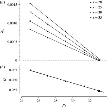This is illustrated in figure 4(a), which shows the squared amplitude of the mixture-fraction oscillations along the axis at four different downstream locations, as obtained in numerical simulations for $\mathit{Re}=50$ , $S=4.62$ and decreasing values of $\mathit{Fr}$ . Extrapolating the corresponding results to zero amplitude provides the critical value $\mathit{Fr}^{\ast }$ of $\mathit{Fr}$ , giving for instance $\mathit{Fr}^{\ast }=(33,305,940)$ for $\mathit{Re}=(50,100,150)$ . These values are compared in figure 3 with the values $\mathit{Fr}^{\ast }=(26.60,261.40,745.64)$ corresponding to the linear stability analysis.

The direct numerical simulations also indicate that near the margin of stability there exists a linear dependence of the oscillation frequency on the Froude number. As shown in figure 4(b), the observed frequency is identical at all four locations – confirming the global nature of the flicker instability – with the critical value $\mathit{St}^{\ast }=0.054$ approached as $\mathit{Fr}\rightarrow \mathit{Fr}^{\ast }\simeq 33$ . This is to be compared with the value $\mathit{St}=0.0628$ predicted by the global stability analysis at the corresponding critical Froude number $\mathit{Fr}=26.60$ . The differences observed, for both critical Froude numbers and associated frequencies, whose relative magnitude is of the order of 20 % in the range of Reynolds numbers investigated, may be attributed to the fact that disturbances experience very large gains in slightly subcritical settings, leading to a substantial amplification of small numerical noise in the DNS integrations that results in the larger critical values of $\mathit{Fr}$ shown in figure 3. Clearly, the origin of the observed discrepancies warrants further investigation in future work.

Figure 4.

DNS computations of the (a) squared amplitude of oscillations, $A^{2}$ , and (b) Strouhal numbers $\mathit{St}$ , measured at different downstream axial locations, $x=20,25,30$ and $35$ for $\mathit{Re}=50$ and $S=4.62$ . The solid lines in the upper part of the plot represent linear fits of the points $(\mathit{Fr},A^{2})$ in order to determine the critical Froude number, $\mathit{Fr}^{\ast }$ , for which the amplitude of the oscillations is zero. Upon extrapolation, a critical value $\mathit{Fr}^{\ast }=33.065$ was found, with an associated Strouhal number $\mathit{St}^{\ast }=0.0544$ , marked with a cross, whereas the Strouhal number for the conditions predicted by the global stability analysis was found to be $\mathit{St}=0.0628$ .

5 Comparison with a local stability analysis

As explained in Huerre & Monkewitz (Reference Huerre and Monkewitz1990), for slender flows there exists a close relationship between the evolution of the local stability characteristics at each streamwise position $x$ and the global instability properties of the flow. However, this relationship depends crucially on the requirement that the wavelength ${\it\lambda}$ be much smaller than the typical evolution length scale $L$ of the basic flow; and, quoting Huerre & Monkewitz (Reference Huerre and Monkewitz1990), ‘A breakdown of this assumption would preclude any possible connection between local and global instability properties’. For the diffusion flame presented in figure 3, it can be seen that the wavelength  ${\it\lambda}$ of the global instability is comparable to the flame height, which characterizes the spatial evolution of the base flow. Therefore, the conditions needed for applicability of the local spatio-temporal analysis are not satisfied, which may result in significant inaccuracies in inferred predictions of global instability properties. This aspect of the problem is to be investigated here. Specifically, we shall study the downstream evolution of the local spatio-temporal stability properties of the base flow used earlier for the global stability analysis. We begin by formulating the local stability analysis, and then show results for the case $S=6.1$ and $\mathit{Re}=75$ , with $\mathit{Fr}=375$ and $\mathit{Fr}=800$ . In analysing the results it is worth bearing in mind that the global instability analysis predicts a critical Froude number $\mathit{Fr}=368$ for $S=6.1$ and $\mathit{Re}=75$ , so that the flow should be globally stable under these conditions.

At each downstream position $x$ , the basic flow is assumed to be locally parallel, with radial profiles of velocity $\bar{\boldsymbol{v}}(r)=(\bar{v}_{x}(r),0)$ and mixture fraction $\bar{Z}(r)$ ; small perturbations are introduced as normal modes $[\tilde{v}_{x}(r),\text{i}\tilde{v}_{r}(r),\tilde{p}(r),\tilde{Z}(r)]\exp [\text{i}(kx-{\it\omega}t)]$ , with complex axial wavenumber $k=k_{r}+\text{i}k_{i}$ and complex angular frequency ${\it\omega}={\it\omega}_{r}+\text{i}{\it\omega}_{i}$ . Here $k$ , ${\it\omega}$ , and $t$ are non-dimensionalized using $a$ and $U_{0}$ . In appendix A.1 it is shown how substitution of the normal modes into the equations of motion (2.4)–(2.6), linearized around the steady base flow, yields the system of ordinary differential equations (A 1)–(A 4) that, together with the boundary conditions (A 11)–(A 12), provides a generalized eigenvalue problem. The local stability properties can be obtained by solving the latter, whereby eigenfunctions $\tilde{v}_{x}(r)$ , $\tilde{v}_{r}(r)$ , $\tilde{p}(r)$ , $\tilde{Z}(r)$ only exist if $k$ and ${\it\omega}$ satisfy a dispersion relation $D(k,{\it\omega};\mathit{Re},\mathit{Fr},S,{\it\gamma},\ldots ,\bar{v}_{x},\bar{v}_{r},\bar{p},\bar{Z})=0$ . In the present section we are concerned with the absolute or convective character of the instability. Therefore we need to find the spatio-temporal instability modes with zero group velocity, i.e. modes for which $\text{d}{\it\omega}/\text{d}k=0$ . The growth rate ${\it\omega}_{0,i}$ of these is called the absolute growth rate and determines whether the instability is convective, ${\it\omega}_{0,i}<0$ , or absolute, ${\it\omega}_{0,i}>0$ . The condition $\text{d}{\it\omega}/\text{d}k=0$ is equivalent to the existence of a double root, or saddle point, in the complex $k$ -plane, $\partial D/\partial k|_{k=k_{0}}=0$ . Among all the saddle points that may exist, only the one with the largest value of ${\it\omega}_{0,i}$ , while satisfying the Briggs–Bers criterion, determines the large-time impulse response of the flow (see, for instance, Huerre Reference Huerre, Batchelor, Moffatt and Worster2000, and references therein). The numerical method used to determine $({\it\omega}_{0},k_{0})$ is described in appendix A.2.

Figure 5.

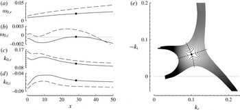
(a–d) Downstream evolution of the local spatio-temporal stability properties for $S=6.1$ and $\mathit{Re}=75$ , with $\mathit{Fr}=800$ (solid line) and $\mathit{Fr}=375$ (dashed line). (e) Location of the saddle point $({\it\omega}_{0},k_{0})$ in the complex $k$ -plane at the downstream position $x=28.4$ , as indicated in (a–d) by the dots; the solid lines are spatial branches with a constant value of ${\it\omega}_{i}$ ; the dashed lines are lines of constant ${\it\omega}_{r}={\it\omega}_{0,r}$ .

Figure 5(a–d) show the downstream evolution of the spatio-temporal stability properties for the case $S=6.1$ and $\mathit{Re}=75$ , with two values of the Froude number: $\mathit{Fr}=800$ (solid lines) and $\mathit{Fr}=375$ (dashed lines). The location of the saddle point $k=k_{0}$ in the complex $k$ -plane is shown in figure 5(e), where the solid lines indicate spatial branches of constant ${\it\omega}_{i}$ and the dashed lines have a constant value of ${\it\omega}_{i}={\it\omega}_{0,i}$ . It can be seen how, for $\mathit{Fr}\lesssim 800$ , a pocket of absolute instability emerges around $x=28$ , with absolute frequency ${\it\omega}_{0,r}=0.02$ ( $\mathit{St}=0.006$ ) and wavelength ${\it\lambda}_{0}=2{\rm\pi}/k_{0,r}=63$ . In numerical simulations of weakly non-parallel heated jets, the appearance of such a pocket of absolute instability was shown to destabilize the nonlinear global mode responsible for the self-excited behaviour (Lesshafft et al. Reference Lesshafft, Huerre and Sagaut2007). Moreover, at criticality, the corresponding global frequency was found to coincide with the value given by the local stability analysis at the downstream position where the character of the instability changes from convective to absolute, in agreement with the theory developed by Pier, Huerre & Chomaz (Reference Pier, Huerre and Chomaz1998) for weakly non-parallel flows.

The spatio-temporal stability analysis therefore predicts the flow to be globally unstable for $\mathit{Fr}\lesssim 800$ , with a frequency at the margin of instability such that $\mathit{St}=0.006$ . These predictions differ significantly from those of the global stability analysis, which gives a critical Froude number $\mathit{Fr}=368$ with an associated Strouhal number $\mathit{St}\simeq 0.014$ . These departures can be attributed to the failure of the condition ${\it\lambda}\ll L$ needed for applicability of the quasi-parallel analysis. Similar overpredictions in the growth rate of the perturbations have been reported in previous comparative studies of local/global stability analyses for wakes (Juniper, Tammisola & Lundell Reference Juniper, Tammisola and Lundell2011).

A pocket of absolutely unstable flow, away from boundaries, was also found by Qadri et al. (Reference Qadri, Chandler and Juniper2015) in the context of non-buoyant flames for their ‘mode B’. As in the present work, they found this region of local absolute instability to lie at the basis of the excitation of a global low-frequency flickering mode. In the buoyancy-free configuration analysed by Qadri et al. (Reference Qadri, Chandler and Juniper2015) the density of the fuel jet upstream from the lifted flame is significantly lower than that of the surrounding atmosphere, causing a second instability mode (‘mode A’) to be present in their analysis, with a region of absolute instability that starts at the outlet of the jet, similar to that found by Coenen & Sevilla (Reference Coenen and Sevilla2012) in the context of light jets.