2.1. A ternary phase diagram

A ternary phase diagram determines the solid and liquid phases present in local thermodynamic equilibrium at a given temperature and bulk composition. For a detailed description of ternary phase diagrams, see e.g. West (Reference West1982). Related theoretical studies on diffusion-limited (Anderson Reference Anderson2003) and convective (Anderson & Schulze Reference Anderson and Schulze2005) regimes of ternary-alloy solidification consider an idealized ternary phase diagram based on the two principal simplifications: there is complete immiscibility in the solid phase (no solid solutions form) and all liquidus surfaces are planar. Here, as in Anderson et al. (Reference Anderson, McFadden, Coriell and Murray2010), we relax the first assumption by considering a partial solid miscibility, giving rise to the formation of solid solutions rather than pure solid phases.

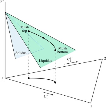
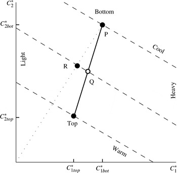
Figure 1 depicts a perspective sketch of the ternary phase diagram under consideration. We consider a ternary alloy of components 1, 2 and 3, and denote the liquid compositions of components 1, 2 and 3 by $C_{1}^{\ast }$ , $C_{2}^{\ast }$ and $C_{3}^{\ast }$ , noting that $C_{1}^{\ast }+C_{2}^{\ast }+C_{3}^{\ast }=1$ . The three corners of a compositional base of the phase diagram correspond to the pure components 1, 2 and 3 of the alloy. A portion of the phase diagram shown in figure 1 is chosen to correspond to the corner 3 of the full ternary phase diagram. We address the evolution of a ternary alloy along the liquidus surface of the phase diagram and the associated formation of a primary mushy layer. The solid phase forming the dendrites in the mushy layer is a solid solution, made up primarily of component 3 of the alloy, with components 1 and 2 incorporated; there is a partial rejection of the alloy components into the residual liquid. The solid compositions are determined by the solidus surface at a given temperature and are related to the liquid compositions by $k_{j}C_{j}^{\ast }$ , where $k_{j}$ is a constant segregation coefficient for component $j$ (  $j=1,2$ ). We denote the local volume fraction of the solid in the mushy layer by ${\it\phi}$ . We invoke an additional simplification that there is no formation of secondary and tertiary solid phases or intercrystalline compounds. The caption to figure 1 describes the features of the phase diagram in further detail.

Figure 1.

A schematic of the ternary phase diagram. The three corners of a triangular base of the phase diagram correspond to the pure components 1, 2 and 3 of the ternary alloy. The liquidus surface and the solidus surface associated with the corner 3 are illustrated. A typical solidification path and its projection onto the base of the diagram are also depicted, indicating the phase trajectory of ternary melt as it descends along the liquidus surface. The solidification path corresponds to the formation of a primary mushy layer made up of dendrites of a component-3-rich solid phase surrounded by the residual liquid. In an ideal primary mushy layer, both the liquidus and solidus surfaces are taken to be planar.

2.2. Dimensional governing equations

The model we analyse here is that introduced by Anderson et al. (Reference Anderson, McFadden, Coriell and Murray2010). The present formulation and notation are similar to theirs. For clarity, we start with the governing equations and boundary conditions in dimensional units. We only sketch the main aspects of the model; full details are given in Anderson et al. (Reference Anderson, McFadden, Coriell and Murray2010).

We consider a two-dimensional system in which a ternary alloy is solidifying at a constant rate $V^{\ast }$ . There is a primary mushy layer in the region $0<z^{\ast }<H^{\ast }$ , where the mushy-layer thickness $H^{\ast }$ is assumed to be a given constant. The liquid compositions at the top of the mushy layer are $C_{1\mathit{top}}^{\ast }$ and $C_{2\mathit{top}}^{\ast }$ while those at the bottom are $C_{1\mathit{bot}}^{\ast }$ and $C_{2\mathit{bot}}^{\ast }$ , each of which is assumed constant. The temperatures at the top and bottom boundaries, $T_{\mathit{top}}^{\ast }$ and $T_{\mathit{bot}}^{\ast }$ , are then specified by a single liquidus surface of the equilibrium ternary phase diagram, which is here taken to be associated with corner 3 and also assumed to be away from any cotectic curves or eutectic points. We view the system from a frame of reference fixed to the bottom of the mush, in which the solid phase formed within the mush is moving downwards with the background solidification speed  $V^{\ast }$ . For simplicity, the thermal properties, the specific heat and the thermal conductivity, are assumed to be the same in the solid and liquid phases.

The equations governing the primary mushy layer are the thermal balance, two solute balances, ternary liquidus constraint, Darcy’s equation and mass balance given by

(2.1a ) $$\begin{eqnarray}c^{\ast }\left(\frac{\partial T^{\ast }}{\partial t^{\ast }}-V^{\ast }\frac{\partial T^{\ast }}{\partial z^{\ast }}\right)+c^{\ast }\boldsymbol{u}^{\ast }\boldsymbol{\cdot }\boldsymbol{{\rm\nabla}}^{\ast }T^{\ast }=k^{\ast }{\rm\nabla}^{\ast 2}T^{\ast }+L_{v}^{\ast }\left(\frac{\partial {\it\phi}}{\partial t^{\ast }}-V^{\ast }\frac{\partial {\it\phi}}{\partial z^{\ast }}\right),\end{eqnarray}$$

(2.1b ) $$\begin{eqnarray}\displaystyle & & \displaystyle \displaystyle \left(1-{\it\phi}\right)\left(\frac{\partial C_{j}^{\ast }}{\partial t^{\ast }}-V^{\ast }\frac{\partial C_{j}^{\ast }}{\partial z^{\ast }}\right)+\boldsymbol{u}^{\ast }\boldsymbol{\cdot }\boldsymbol{{\rm\nabla}}^{\ast }C_{j}^{\ast }=D_{j}^{\ast }\boldsymbol{{\rm\nabla}}^{\ast }\boldsymbol{\cdot }\left[\left(1-{\it\phi}\right)\boldsymbol{{\rm\nabla}}^{\ast }C_{j}^{\ast }\right]\nonumber\\ \displaystyle & & \displaystyle \displaystyle \quad +\left(1-k_{j}\right)C_{j}^{\ast }\left(\frac{\partial {\it\phi}}{\partial t^{\ast }}-V^{\ast }\frac{\partial {\it\phi}}{\partial z^{\ast }}\right),\quad \text{for }j=1,2,\end{eqnarray}$$

(2.1c ) $$\begin{eqnarray}\displaystyle & \displaystyle T^{\ast }=T_{\mathit{top}}^{\ast }+m_{1}^{\ast }\left(C_{1}^{\ast }-C_{1\mathit{top}}^{\ast }\right)+m_{2}^{\ast }\left(C_{2}^{\ast }-C_{2\mathit{top}}^{\ast }\right), & \displaystyle\end{eqnarray}$$

(2.1d ) $$\begin{eqnarray}\displaystyle & \displaystyle \boldsymbol{u}^{\ast }=-\frac{{\it\Pi}^{\ast }\left({\it\phi}\right)}{{\it\mu}^{\ast }}\big(\boldsymbol{{\rm\nabla}}^{\ast }p^{\ast }+{\rm\Delta}{\it\rho}^{\ast }g^{\ast }\hat{\boldsymbol{k}}\big), & \displaystyle\end{eqnarray}$$

(2.1e ) $$\begin{eqnarray}\displaystyle & \displaystyle \boldsymbol{{\rm\nabla}}^{\ast }\boldsymbol{\cdot }\boldsymbol{u}^{\ast }=0. & \displaystyle\end{eqnarray}$$

$T^{\ast }$

$C_{1}^{\ast }$

$C_{2}^{\ast }$

${\it\phi}$

$p^{\ast }$

$p^{\ast }=p_{\mathit{dyn}}+{\it\rho}_{\mathit{top}}^{\ast }g^{\ast }z^{\ast }$

$\boldsymbol{u}^{\ast }$

$c^{\ast }$

$k^{\ast }$

$L_{v}^{\ast }$

$D_{j}^{\ast }$

$j$

$k_{j}$

$j$

$m_{j}^{\ast }$

${\it\Pi}^{\ast }({\it\phi})$

${\it\mu}^{\ast }$

$g^{\ast }$

$\hat{\boldsymbol{k}}$

Convective motions in the mush are driven by a density differential ${\rm\Delta}{\it\rho}^{\ast }={\it\rho}^{\ast }-{\it\rho}_{\mathit{top}}^{\ast }$ in (2.1d ), with the density assumed to be linearly related to the temperature and compositions,

(2.2) $$\begin{eqnarray}{\it\rho}^{\ast }={\it\rho}_{\mathit{top}}^{\ast }\left[1-{\it\alpha}^{\ast }\left(T^{\ast }-T_{\mathit{top}}^{\ast }\right)-{\it\alpha}_{1}^{\ast }\left(C_{1}^{\ast }-C_{1\mathit{top}}^{\ast }\right)-{\it\alpha}_{2}^{\ast }\left(C_{2}^{\ast }-C_{2\mathit{top}}^{\ast }\right)\right],\end{eqnarray}$$

where ${\it\alpha}^{\ast }$ and ${\it\alpha}_{j}^{\ast }$ (  $j=1,2$ ) are the thermal and compositional expansion coefficients, respectively. It should be noted that, since the variables $T^{\ast }$ , $C_{1}^{\ast }$ and $C_{2}^{\ast }$ are related by the ternary liquidus constraint (2.1c ), we could eliminate either of $T^{\ast }$ , $C_{1}^{\ast }$ or $C_{2}^{\ast }$ from direct consideration.

These equations are subject to the following boundary conditions:

(2.3a−d ) $$\begin{eqnarray}C_{1}^{\ast }=C_{1\mathit{top}}^{\ast },\quad C_{2}^{\ast }=C_{2\mathit{top}}^{\ast },\quad {\it\phi}={\it\phi}_{0},\quad \boldsymbol{u}^{\ast }\boldsymbol{\cdot }\hat{\boldsymbol{k}}=0\quad \text{at }z^{\ast }=H^{\ast },\end{eqnarray}$$

(2.4a−c ) $$\begin{eqnarray}C_{1}^{\ast }=C_{1\mathit{bot}}^{\ast },\quad C_{2}^{\ast }=C_{2\mathit{bot}}^{\ast },\quad \boldsymbol{u}^{\ast }\boldsymbol{\cdot }\hat{\boldsymbol{k}}=0\quad \text{at }z^{\ast }=0,\end{eqnarray}$$

where $C_{jtop}^{\ast }$ , $C_{jbot}^{\ast }$ (  $j=1,2$ ) and ${\it\phi}_{0}$ are prescribed constants. It should be noted that, in light of (2.1c ), the temperature is automatically $T_{\mathit{top}}^{\ast }$ at the mush top, while the temperature at the mush bottom attains a dependent value $T_{\mathit{bot}}^{\ast }=T_{\mathit{top}}^{\ast }+m_{1}^{\ast }\left(C_{1\mathit{bot}}^{\ast }-C_{1\mathit{top}}^{\ast }\right)+m_{2}^{\ast }\left(C_{2\mathit{bot}}^{\ast }-C_{2\mathit{top}}^{\ast }\right)$ . Thus, the boundary conditions (2.3) and (2.4) are sufficient. As described in Anderson et al. (Reference Anderson, McFadden, Coriell and Murray2010), these boundary conditions effectively decouple the primary mushy layer from the dynamics of any adjacent layers (an overlying liquid layer, an underlying secondary mushy layer or a eutectic solid layer), thus simplifying the mathematical analysis of the essential interactions internal to the primary mushy layer.

2.3. Dimensionless governing equations

Here we recast the equations governing the primary mush in dimensionless form. In the present analysis, we adopt a different scheme of non-dimensionalization from that in Anderson et al. (Reference Anderson, McFadden, Coriell and Murray2010). Specifically, we define a dimensionless temperature $T$ and compositions $C_{j}$ ,

(2.5a,b ) $$\begin{eqnarray}T=\frac{T^{\ast }-T_{\mathit{top}}^{\ast }}{{\rm\Delta}T^{\ast }},\quad C_{j}=\frac{C_{j}^{\ast }-C_{jtop}^{\ast }}{{\rm\Delta}C_{j}^{\ast }},\end{eqnarray}$$

where ${\rm\Delta}T^{\ast }=T_{\mathit{top}}^{\ast }-T_{\mathit{bot}}^{\ast }$ and ${\rm\Delta}C_{j}^{\ast }=C_{jtop}^{\ast }-C_{jbot}^{\ast }$ (  $j=1,2$ ). The velocity is non-dimensionalized using $V^{\ast }$ , space and time by the thermal diffusion length and time ${\it\kappa}^{\ast }/V^{\ast }$ and ${\it\kappa}^{\ast }/V^{\ast 2}$ , respectively, where ${\it\kappa}^{\ast }=k^{\ast }/c^{\ast }$ is the thermal diffusivity, the reduced pressure by the factor ${\it\mu}^{\ast }{\it\kappa}^{\ast }/{\it\Pi}^{\ast }\left({\it\phi}_{0}\right)$ , where ${\it\Pi}^{\ast }\left({\it\phi}_{0}\right)$ is a permeability scale, and the density differential by the scale ${\it\mu}^{\ast }V^{\ast }/\left(g^{\ast }{\it\Pi}^{\ast }\left({\it\phi}_{0}\right)\right)$ . The dimensionless form of the governing equations is then

(2.6a ) $$\begin{eqnarray}\displaystyle & \displaystyle \left(\frac{\partial }{\partial t}-\frac{\partial }{\partial z}\right)T+\boldsymbol{u}\boldsymbol{\cdot }\boldsymbol{{\rm\nabla}}T={\rm\nabla}^{2}T+S\left(\frac{\partial }{\partial t}-\frac{\partial }{\partial z}\right){\it\phi}, & \displaystyle\end{eqnarray}$$

(2.6b ) $$\begin{eqnarray}\displaystyle & \displaystyle (1-{\it\phi})\left(\frac{\partial }{\partial t}-\frac{\partial }{\partial z}\right)C_{j}+\boldsymbol{u}\boldsymbol{\cdot }\boldsymbol{{\rm\nabla}}C_{j}\hspace{230.39996pt} & \displaystyle \nonumber\\ \displaystyle & \displaystyle =\frac{1}{\mathit{Le}_{j}}\boldsymbol{{\rm\nabla}}\boldsymbol{\cdot }[(1-{\it\phi})\boldsymbol{{\rm\nabla}}C_{j}]+(1-k_{j})(1+C_{j}^{bot}+C_{j})\!\left(\frac{\partial }{\partial t}-\frac{\partial }{\partial z}\right)\!{\it\phi},\quad \text{for }j=1,2,\qquad & \displaystyle\end{eqnarray}$$

(2.6c ) $$\begin{eqnarray}\displaystyle & \displaystyle T=m_{1}C_{1}+m_{2}C_{2}, & \displaystyle\end{eqnarray}$$

(2.6d ) $$\begin{eqnarray}\displaystyle & \displaystyle K({\it\phi})\boldsymbol{u}=-\boldsymbol{{\rm\nabla}}p-{\rm\Delta}{\it\rho}\,\hat{\boldsymbol{k}}, & \displaystyle\end{eqnarray}$$

(2.6e ) $$\begin{eqnarray}\displaystyle & \displaystyle \boldsymbol{{\rm\nabla}}\boldsymbol{\cdot }\boldsymbol{u}=0, & \displaystyle\end{eqnarray}$$

$K({\it\phi})={\it\Pi}^{\ast }({\it\phi}_{0})/{\it\Pi}^{\ast }({\it\phi})$

(2.7) $$\begin{eqnarray}{\rm\Delta}{\it\rho}=-RaT-Ra_{1}C_{1}-Ra_{2}C_{2}.\end{eqnarray}$$

The dimensionless parameters appearing in these equations are the Stefan number $S$ , the Lewis numbers $\mathit{Le}_{j}$ , the concentration ratios $C_{j}^{bot}$ , the liquidus surface slopes $m_{j}$ , the thermal Rayleigh number $Ra$ and the compositional Rayleigh numbers $Ra_{j}$ , defined by

(2.8a−d ) $$\begin{eqnarray}S=\frac{L_{v}^{\ast }}{c^{\ast }{\rm\Delta}T^{\ast }},\quad \mathit{Le}_{j}=\frac{{\it\kappa}^{\ast }}{D_{j}^{\ast }},\quad C_{j}^{bot}=\frac{C_{jbot}^{\ast }}{{\rm\Delta}C_{j}^{\ast }},\quad m_{j}=\frac{m_{j}^{\ast }{\rm\Delta}C_{j}^{\ast }}{{\rm\Delta}T^{\ast }},\end{eqnarray}$$

(2.9a,b ) $$\begin{eqnarray}Ra=\frac{{\it\rho}_{\mathit{top}}^{\ast }{\it\alpha}^{\ast }{\rm\Delta}T^{\ast }g^{\ast }{\it\Pi}^{\ast }({\it\phi}_{0})}{{\it\mu}^{\ast }V^{\ast }},\quad Ra_{j}=\frac{{\it\rho}_{\mathit{top}}^{\ast }{\it\alpha}_{j}^{\ast }{\rm\Delta}C_{j}^{\ast }g^{\ast }{\it\Pi}^{\ast }({\it\phi}_{0})}{{\it\mu}^{\ast }V^{\ast }},\end{eqnarray}$$

for $j=1,2$ . It should be noted that, from the liquidus constraint (2.1c ) considered at the bottom of the mush, the slopes $m_{1}$ and $m_{2}$ are not independent but are related by $m_{1}+m_{2}=1$ .

Equations (2.6) are subject to the boundary conditions

(2.10a−d ) $$\begin{eqnarray}C_{1}=0,\quad C_{2}=0,\quad {\it\phi}={\it\phi}_{0},\quad \boldsymbol{u}\boldsymbol{\cdot }\hat{\boldsymbol{k}}=0\quad \text{at }z={\it\delta},\end{eqnarray}$$

(2.11a−c ) $$\begin{eqnarray}C_{1}=-1,\quad C_{2}=-1,\quad \boldsymbol{u}\boldsymbol{\cdot }\hat{\boldsymbol{k}}=0\quad \text{at }z=0.\end{eqnarray}$$

Conditions (2.10) contain one additional parameter: the dimensionless thickness of the mushy layer, defined by

(2.12) $$\begin{eqnarray}{\it\delta}=\frac{H^{\ast }}{{\it\kappa}^{\ast }/V^{\ast }}.\end{eqnarray}$$

It should be noted that the parameter ${\it\delta}$ can also be considered as a scaled pulling speed (denoted as $V$ in Anderson et al. Reference Anderson, McFadden, Coriell and Murray2010; see their equation (2.8a)).

In (2.7) we eliminate $T$ in favour of $C_{1}$ and $C_{2}$ so that

(2.13) $$\begin{eqnarray}{\rm\Delta}{\it\rho}=-Ra_{C1}C_{1}-Ra_{C2}C_{2},\end{eqnarray}$$

depending only on the two effective compositional Rayleigh numbers

(2.14) $$\begin{eqnarray}Ra_{Cj}=m_{j}Ra+Ra_{j},\quad \text{for }j=1,2.\end{eqnarray}$$

It should be noted that $Ra_{C1}+Ra_{C2}=Ra+Ra_{1}+Ra_{2}$ .

Formulation of the problem is completed by a choice of the function $K({\it\phi})$ . We discuss this choice in § 3.2.

2.4. Rescaling

The model is reduced asymptotically by restricting the primary mush thickness to be thin by letting ${\it\delta}\ll 1$ . This means that the dimensional mush thickness is much less than the thermal diffusive length; equivalently, the dimensional pulling speed is much smaller than the rate of heat transfer across the layer by thermal conduction.

The particular physical effect that gave rise to convective instabilities in the Anderson et al. (Reference Anderson, McFadden, Coriell and Murray2010) simple-model analysis was that associated with the phase change influence on the net solute balance through solute diffusion. Here, in addition to all the diffusive processes, we wish to isolate a variety of other phase change effects, in particular the rejection of two solutes and the release of latent heat, at dominant order in the limit of small ${\it\delta}$ . These physical effects underpin the rescalings to follow.

We consider the limits where $C_{j}^{bot}$ and $S$ are large by writing

(2.15a,b ) $$\begin{eqnarray}C_{j}^{bot}=\frac{\bar{C}_{j}^{bot}}{{\it\delta}^{2}},\quad S=\frac{\bar{S}}{{\it\delta}^{2}},\end{eqnarray}$$

where $\bar{C}_{j}^{bot}$ and $\bar{S}$ are $O(1)$ as ${\it\delta}\rightarrow 0$ , for $j=1,2$ . Physically, the scaling for $C_{j}^{bot}$ corresponds to relatively weak compositional variations in the two solute components across the mush, and enables the dynamics of the system to take place away from binary sides of the ternary phase diagram. The scaling for $S$ assumes that the latent heat released on local phase change is much greater than the heat associated with the mush temperature drop. We note in passing that a regime where $C_{j}^{bot}$ and $S$ are  $O(1/{\it\delta})$ , in analogy to binary mushy-layer systems with no solute diffusion (Anderson & Worster Reference Anderson and Worster1995, Reference Anderson and Worster1996), turns out to be inappropriate when solute diffusion is included; this is discussed further in the final paragraph of appendix B.

Next, we rescale space and time, and introduce new scaled Rayleigh numbers as

(2.16a,b ) $$\begin{eqnarray}(x,z)={\it\delta}(\bar{x},\bar{z}),\quad t={\it\delta}^{2}\bar{t},\end{eqnarray}$$

(2.17a,b ) $$\begin{eqnarray}Ra=\frac{1}{{\it\delta}}\overline{Ra},\quad Ra_{j}=\frac{1}{{\it\delta}}\overline{Ra}_{j},\end{eqnarray}$$

for $j=1,2$ , where all the barred quantities are assumed fixed, of $O(1)$ , as ${\it\delta}\rightarrow 0$ . We shall have occasion below to interpret the stability results in terms of the effective Rayleigh numbers and hence conveniently define also their scaled versions by $\overline{Ra}_{Cj}=m_{j}\overline{Ra}+\overline{Ra}_{j}$ for $j=1,2$ (cf. (2.14)). It should be noted that, as implied by (2.17), the scaled Rayleigh numbers $\overline{Ra}$ , $\overline{Ra}_{1}$ and $\overline{Ra}_{2}$ are based on the thermal diffusive length scale, rather than the actual mush thickness employed in the original definitions (2.9). Hence $\overline{Ra}$ , $\overline{Ra}_{1}$ and $\overline{Ra}_{2}$ in our analysis are identical to $Ra$ , $Ra_{1}$ and $Ra_{2}$ in Anderson et al. (Reference Anderson, McFadden, Coriell and Murray2010).

3.1. Steady non-convecting solution

Here, we present an asymptotic solution for the non-convecting mushy layer. This base-state solution is steady, horizontally uniform and satisfies

(3.2a ) $$\begin{eqnarray}-{\it\delta}\frac{\text{d}}{\text{d}\bar{z}}\left(\tilde{T}-\frac{1}{{\it\delta}^{2}}\bar{S}\tilde{{\it\phi}}\right)=\frac{\text{d}^{2}\tilde{T}}{\text{d}\bar{z}^{2}},\end{eqnarray}$$

(3.2b ) $$\begin{eqnarray}\displaystyle -{\it\delta}\big(1-\tilde{{\it\phi}}\big)\frac{\text{d}\tilde{C}_{j}}{\text{d}\bar{z}} & = & \displaystyle \frac{1}{\mathit{Le}_{j}}\frac{\text{d}}{\text{d}\bar{z}}\left[\big(1-\tilde{{\it\phi}}\big)\frac{\text{d}\tilde{C}_{j}}{\text{d}\bar{z}}\right]\nonumber\\ \displaystyle & & \displaystyle -\,{\it\delta}(1-k_{j})\left(1+\frac{1}{{\it\delta}^{2}}\bar{C}_{j}^{bot}+\tilde{C}_{j}\right)\frac{\text{d}\tilde{{\it\phi}}}{\text{d}\bar{z}},\quad \text{for }j=1,2,\end{eqnarray}$$

(3.2c ) $$\begin{eqnarray}\tilde{T}=m_{1}\tilde{C}_{1}+m_{2}\tilde{C}_{2},\end{eqnarray}$$

(3.3a−c ) $$\begin{eqnarray}\tilde{C}_{1}=0,\quad \tilde{C}_{2}=0,\quad \tilde{{\it\phi}}={\it\phi}_{0}\quad \text{at }\bar{z}=1,\end{eqnarray}$$

(3.4a,b ) $$\begin{eqnarray}\tilde{C}_{1}=-1,\quad \tilde{C}_{2}=-1\quad \text{at }\bar{z}=0.\end{eqnarray}$$

An equation for $\tilde{p}$ will not be needed explicitly.

We solve these equations asymptotically in terms of regular expansions in powers of ${\it\delta}$ , namely

(3.5) $$\begin{eqnarray}\tilde{T}=\tilde{T}^{0}+{\it\delta}\,\tilde{T}^{1}+\cdots \,,\end{eqnarray}$$

and similarly for other base-state quantities $\tilde{C}_{1}$ , $\tilde{C}_{2}$ and $\tilde{{\it\phi}}$ . The solution is

(3.6a ) $$\begin{eqnarray}\displaystyle & \displaystyle \tilde{T}=-\left(1-\bar{z}\right)+{\it\delta}{\textstyle \frac{1}{2}}{\it\Omega}\bar{z}\left(1-\bar{z}\right)+\cdots \,, & \displaystyle\end{eqnarray}$$

(3.6b ) $$\begin{eqnarray}\displaystyle & \displaystyle \tilde{C}_{j}=-\left(1-\bar{z}\right)+{\it\delta}{\textstyle \frac{1}{2}}{\it\Omega}_{j}\bar{z}\left(1-\bar{z}\right)+\cdots \,, & \displaystyle\end{eqnarray}$$

(3.6c ) $$\begin{eqnarray}\displaystyle & \displaystyle \tilde{{\it\phi}}={\it\phi}_{0}-{\it\delta}^{2}\frac{1}{{\it\Gamma}}\left(1-\bar{z}\right)+\cdots \,, & \displaystyle\end{eqnarray}$$

(3.7a,b ) $$\begin{eqnarray}{\it\Omega}=1-\frac{\bar{S}}{{\it\Gamma}},\quad {\it\Omega}_{j}=1-\frac{{\it\Gamma}_{j}}{{\it\Gamma}},\end{eqnarray}$$

for $j=1,2$ , with

(3.8a ) $$\begin{eqnarray}\displaystyle & \displaystyle {\it\Gamma}=-\frac{m_{1}\mathit{Le}_{1}\mathscr{C}_{1}+m_{2}\mathit{Le}_{2}\mathscr{C}_{2}-(1-{\it\phi}_{0})\bar{S}}{(1-{\it\phi}_{0})(1-m_{1}\mathit{Le}_{1}-m_{2}\mathit{Le}_{2})}, & \displaystyle\end{eqnarray}$$

(3.8b ) $$\begin{eqnarray}\displaystyle & \displaystyle {\it\Gamma}_{1}=\frac{(1-\mathit{Le}_{1})(1-{\it\phi}_{0})\bar{S}+m_{2}[\mathit{Le}_{1}\mathscr{C}_{1}-\mathit{Le}_{2}\mathscr{C}_{2}+\mathit{Le}_{1}\mathit{Le}_{2}(\mathscr{C}_{2}-\mathscr{C}_{1})]}{(1-{\it\phi}_{0})(1-m_{1}\mathit{Le}_{1}-m_{2}\mathit{Le}_{2})}, & \displaystyle\end{eqnarray}$$

(3.8c ) $$\begin{eqnarray}\displaystyle & \displaystyle {\it\Gamma}_{2}=\frac{(1-\mathit{Le}_{2})(1-{\it\phi}_{0})\bar{S}+m_{1}[\mathit{Le}_{2}\mathscr{C}_{2}-\mathit{Le}_{1}\mathscr{C}_{1}+\mathit{Le}_{1}\mathit{Le}_{2}(\mathscr{C}_{1}-\mathscr{C}_{2})]}{(1-{\it\phi}_{0})(1-m_{1}\mathit{Le}_{1}-m_{2}\mathit{Le}_{2})}. & \displaystyle\end{eqnarray}$$

$k_{j}$

$\bar{C}_{j}^{bot}$

$\mathscr{C}_{j}\equiv (1-k_{j})\bar{C}_{j}^{bot}$

$C_{j}^{bot}=O(1/{\it\delta}^{2})$

$S=O(1/{\it\delta}^{2})$

${\it\delta}\rightarrow 0$

${\it\phi}_{0}$

${\it\delta}\rightarrow 0$

$O({\it\delta}^{1})$

$\tilde{T}$

$\tilde{C}_{1}$

$\tilde{C}_{2}$

$O(1)$

${\it\Omega}$

${\it\Omega}_{1}$

${\it\Omega}_{2}$

$\mathit{Le}_{j}>1$

$\bar{S}>0$

$\mathscr{C}_{j}<0$

${\it\Omega}$

${\it\Omega}_{j}$

${\it\Omega}=m_{1}{\it\Omega}_{1}+m_{2}{\it\Omega}_{2}$

${\it\Omega}_{1}$

${\it\Omega}_{2}$

${\it\Omega}$

${\it\Omega}_{j}$

${\it\Gamma}$

$\tilde{{\it\phi}}$

3.2. Linearized disturbance equations

The linearized equations governing the perturbation amplitudes are

(3.9a ) $$\begin{eqnarray}\left({\it\sigma}-{\it\delta}\text{D}\right)\left(\hat{T}-\frac{1}{{\it\delta}}\bar{S}\hat{{\it\phi}}\right)+{\hat{w}}\,\text{D}\tilde{T}=\left(\text{D}^{2}-k^{2}\right)\hat{T},\end{eqnarray}$$

(3.9b ) $$\begin{eqnarray}\displaystyle & & \displaystyle \displaystyle \big(1-\tilde{{\it\phi}}\big)\left({\it\sigma}-{\it\delta}\text{D}\right){\hat{C}}_{j}+{\it\delta}^{2}\hat{{\it\phi}}\,\text{D}\tilde{C}_{j}+{\hat{w}}\,\text{D}\tilde{C}_{j}\nonumber\\ \displaystyle & & \displaystyle \displaystyle \quad =\frac{1}{\mathit{Le}_{j}}\left\{\text{D}\big[\big(1-\tilde{{\it\phi}}\big)\text{D}{\hat{C}}_{j}\big]-{\it\delta}\text{D}\big(\hat{{\it\phi}}\,\text{D}\tilde{C}_{j}\big)-k^{2}\big(1-\tilde{{\it\phi}}\big){\hat{C}}_{j}\right\}\nonumber\\ \displaystyle & & \displaystyle \displaystyle \qquad +\left(1-k_{j}\right)\left[{\it\delta}\left(1+\frac{1}{{\it\delta}^{2}}\bar{C}_{j}^{bot}+\tilde{C}_{j}\right)\left({\it\sigma}-{\it\delta}\text{D}\right)\hat{{\it\phi}}-{\it\delta}{\hat{C}}_{j}\,\text{D}\tilde{{\it\phi}}\right],\end{eqnarray}$$

(3.9c ) $$\begin{eqnarray}\displaystyle & \displaystyle \left(\text{D}^{2}-k^{2}\right)\big[K\big(\tilde{{\it\phi}}\big){\hat{w}}\big]+k^{2}\big(\overline{Ra}\hat{T}+\overline{Ra}_{1}{\hat{C}}_{1}+\overline{Ra}_{2}{\hat{C}}_{2}\big)=\text{D}\big[{\hat{w}}\,\text{D}\big[K\big(\tilde{{\it\phi}}\big)\big]\big], & \displaystyle\end{eqnarray}$$

(3.9d ) $$\begin{eqnarray}\displaystyle & \displaystyle \hat{T}=m_{1}{\hat{C}}_{1}+m_{2}{\hat{C}}_{2}, & \displaystyle\end{eqnarray}$$

(3.10a−d ) $$\begin{eqnarray}{\hat{C}}_{1}=0,\quad {\hat{C}}_{2}=0,\quad \hat{{\it\phi}}=0,\quad {\hat{w}}=0\quad \text{at }\bar{z}=1,\end{eqnarray}$$

(3.11a−c ) $$\begin{eqnarray}{\hat{C}}_{1}=0,\quad {\hat{C}}_{2}=0,\quad {\hat{w}}=0\quad \text{at }\bar{z}=0,\end{eqnarray}$$

where $\text{D}\equiv \text{d}/\text{d}\bar{z}$ . In writing (3.9), we have eliminated $\hat{p}$ and ${\hat{u}}$ from direct consideration. It should be noted that, without loss of generality, we may consider two-dimensional disturbances in this linear theory.

Equations (3.9) and boundary conditions (3.10) and (3.11) define a seventh-order non-self-adjoint eigenvalue problem for the growth rate ${\it\sigma}$ . Asymptotic solutions are sought in the form

(3.12a ) $$\begin{eqnarray}\displaystyle & \displaystyle {\it\sigma}={\it\sigma}^{0}+{\it\delta}{\it\sigma}^{1}+\cdots \,, & \displaystyle\end{eqnarray}$$

(3.12b ) $$\begin{eqnarray}\displaystyle & \displaystyle \overline{Ra}=\mathit{Ra}^{0}+{\it\delta}\mathit{Ra}^{1}+\cdots \,, & \displaystyle\end{eqnarray}$$

(3.12c ) $$\begin{eqnarray}\displaystyle & \displaystyle \overline{Ra}_{j}=\mathit{Ra}_{j}^{0}+{\it\delta}\mathit{Ra}_{j}^{1}+\cdots \,, & \displaystyle\end{eqnarray}$$

(3.12d ) $$\begin{eqnarray}\displaystyle & \displaystyle \hat{T}=T^{0}+{\it\delta}T^{1}+\cdots \,, & \displaystyle\end{eqnarray}$$

(3.12e ) $$\begin{eqnarray}\displaystyle & \displaystyle {\hat{C}}_{j}=C_{j}^{0}+{\it\delta}C_{j}^{1}+\cdots \,, & \displaystyle\end{eqnarray}$$

(3.12f ) $$\begin{eqnarray}\displaystyle & \displaystyle \hat{{\it\phi}}={\it\phi}^{0}+{\it\delta}{\it\phi}^{1}+\cdots \,, & \displaystyle\end{eqnarray}$$

(3.12g ) $$\begin{eqnarray}\displaystyle & \displaystyle {\hat{w}}=w^{0}+{\it\delta}w^{1}+\cdots \,. & \displaystyle\end{eqnarray}$$

$K(\tilde{{\it\phi}})$

${\it\phi}_{0}$

${\it\delta}\ll 1$

$\tilde{{\it\phi}}$

$O({\it\delta}^{1})$

(3.13) $$\begin{eqnarray}K(\tilde{{\it\phi}})=1+{\it\delta}^{2}K_{1}\tilde{{\it\phi}}^{2}+\cdots \,,\end{eqnarray}$$

where $K_{1}$ measures the linear permeability variations with base-state solid fraction. Here, we desire this particular physical effect to be captured at $O({\it\delta}^{1})$ in our analysis, and so assume that $K_{1}$ is large, namely

(3.14) $$\begin{eqnarray}K_{1}=\frac{1}{{\it\delta}}\bar{K}_{1},\end{eqnarray}$$

where $\bar{K}_{1}=O(1)$ as ${\it\delta}\rightarrow 0$ . We also require that $\bar{K}_{1}$ is positive so that the permeability decreases with increasing solid fraction.

In a binary-alloy mushy-layer model of Anderson & Worster (Reference Anderson and Worster1995, Reference Anderson and Worster1996) with solute diffusion neglected, the limit appropriate to a thin mushy layer has been shown to effectively reduce the system to one of a non-reactive porous layer with uniform permeability; the physical effects intrinsic to the binary-alloy mushy layer have only appeared as higher-order corrections. In the present ternary-alloy mushy-layer model with finite solute diffusion, in contrast, we find that the leading-order description of the system differs in a variety of ways from the classical (double-diffusive) convection in a non-reactive porous layer, although the leading-order permeability is still uniform (see (3.13)). Specifically, the present system is inherently reactive already at leading order, with the local phase change altering both the heat and solute balances through the physical effects associated with the release of latent heat and the rejection of solutes during local solidification. In § 5, these physical effects are considered further and a formal link with the model of Anderson et al. (Reference Anderson, McFadden, Coriell and Murray2010) is established.

The first equations arise at $O(1/{\it\delta})$ from the heat balance and the two solute balances

(3.15a ) $$\begin{eqnarray}\displaystyle & -{\it\sigma}^{0}\bar{S}{\it\phi}^{0}=0, & \displaystyle\end{eqnarray}$$

(3.15b ) $$\begin{eqnarray}\displaystyle & 0={\it\sigma}^{0}\mathscr{C}_{j}{\it\phi}^{0},\quad \text{for }j=1,2. & \displaystyle\end{eqnarray}$$

${\it\sigma}^{0}=0$

$O({\it\delta}^{1})$

$O({\it\delta}^{2})$

${\it\tau}_{V^{\ast }}^{\ast }=H^{\ast }/V^{\ast }$

${\it\tau}_{{\it\kappa}^{\ast }}^{\ast }=H^{\ast 2}/{\it\kappa}^{\ast }$

${\it\tau}_{{\it\kappa}^{\ast }}^{\ast }/{\it\tau}_{V^{\ast }}^{\ast }={\it\delta}\ll 1$

We proceed to equations at $O({\it\delta}^{0})$ . We eliminate $\hat{T}$ in favour of ${\hat{C}}_{1}$ and ${\hat{C}}_{2}$ from (3.9a,c ) using (3.9d ), use the heat balance thus obtained to eliminate the terms involving $\hat{{\it\phi}}$ in the two solute balances (3.9b ), and combine the resulting solute balances to yield a reduced system

(3.16a ) $$\begin{eqnarray}\displaystyle & \displaystyle \left(\text{D}-{\it\sigma}^{1}\right){\it\phi}^{0}+\frac{1}{{\it\Gamma}\hat{{\it\Gamma}}}w^{0}=0, & \displaystyle\end{eqnarray}$$

(3.16b ) $$\begin{eqnarray}\displaystyle & \displaystyle \left(\text{D}^{2}-k^{2}\right)C_{j}^{0}-\frac{{\it\Omega}_{j}+\hat{{\it\Omega}}_{j}}{1-{\it\phi}_{0}}w^{0}=0,\quad \text{for }j=1,2, & \displaystyle\end{eqnarray}$$

(3.16c ) $$\begin{eqnarray}\displaystyle & \displaystyle \left(\text{D}^{2}-k^{2}\right)w^{0}+k^{2}\big(\mathit{Ra}_{C1}^{0}C_{1}^{0}+\mathit{Ra}_{C2}^{0}C_{2}^{0}\big)=0, & \displaystyle\end{eqnarray}$$

$C_{1}^{0}=C_{2}^{0}={\it\phi}^{0}=w^{0}=0$

$\bar{z}=1$

$C_{1}^{0}=C_{2}^{0}=w^{0}=0$

$\bar{z}=0$

$\mathit{Ra}_{Cj}^{0}=m_{j}Ra^{0}+Ra_{j}^{0}$

${\it\Omega}_{j}$

${\it\Gamma}$

(3.17a ) $$\begin{eqnarray}\displaystyle & \displaystyle \hat{{\it\Omega}}_{j}=-\frac{{\it\phi}_{0}\mathit{Le}_{j}\mathscr{C}_{j}}{m_{1}\mathit{Le}_{1}\mathscr{C}_{1}+m_{2}\mathit{Le}_{2}\mathscr{C}_{2}-\left(1-{\it\phi}_{0}\right)\bar{S}},\quad \text{for }j=1,2, & \displaystyle\end{eqnarray}$$

(3.17b ) $$\begin{eqnarray}\displaystyle & \displaystyle \hat{{\it\Gamma}}=\frac{\left(1-{\it\phi}_{0}\right)\left(1-m_{1}\mathit{Le}_{1}-m_{2}\mathit{Le}_{2}\right)}{1-{\it\phi}_{0}-m_{1}\mathit{Le}_{1}-m_{2}\mathit{Le}_{2}}, & \displaystyle\end{eqnarray}$$

$\hat{{\it\Omega}}_{j}=0$

$\hat{{\it\Gamma}}=1$

${\it\phi}_{0}=0$

$C_{1}^{0}$

$C_{2}^{0}$

$w^{0}$

$\mathit{Ra}_{C1}^{0}$

$\mathit{Ra}_{C2}^{0}$

${\it\phi}^{0}$

The solutions at this order take the form

(3.18a ) $$\begin{eqnarray}\displaystyle & \displaystyle T^{0}=-\sin n{\rm\pi}\bar{z}, & \displaystyle\end{eqnarray}$$

(3.18b ) $$\begin{eqnarray}\displaystyle & \displaystyle C_{j}^{0}=-\frac{{\it\Omega}_{j}+\hat{{\it\Omega}}_{j}}{{\it\Omega}+\hat{{\it\Omega}}}\sin n{\rm\pi}\bar{z},\quad \text{for }j=1,2, & \displaystyle\end{eqnarray}$$

(3.18c ) $$\begin{eqnarray}\displaystyle & \displaystyle {\it\phi}^{0}=\frac{n{\rm\pi}J\left(1-{\it\phi}_{0}\right)}{{\it\Gamma}\hat{{\it\Gamma}}({\it\Omega}+\hat{{\it\Omega}})[n^{2}{\rm\pi}^{2}+({\it\sigma}^{1})^{2}]}\!\left[\left(-1\right)^{n+1}\text{e}^{-{\it\sigma}^{1}\left(1-\bar{z}\right)}+\cos n{\rm\pi}\bar{z}+\frac{{\it\sigma}^{1}}{n{\rm\pi}}\sin n{\rm\pi}\bar{z}\right]\!,\hspace{27.0pt} & \displaystyle\end{eqnarray}$$

(3.18d ) $$\begin{eqnarray}\displaystyle & \displaystyle w^{0}=\frac{J\left(1-{\it\phi}_{0}\right)}{{\it\Omega}+\hat{{\it\Omega}}}\sin n{\rm\pi}\bar{z}, & \displaystyle\end{eqnarray}$$

(3.19) $$\begin{eqnarray}\frac{J^{2}}{k^{2}}+\frac{{\it\Omega}_{1}+\hat{{\it\Omega}}_{1}}{1-{\it\phi}_{0}}\mathit{Ra}_{C1}^{0}+\frac{{\it\Omega}_{2}+\hat{{\it\Omega}}_{2}}{1-{\it\phi}_{0}}\mathit{Ra}_{C2}^{0}=0,\end{eqnarray}$$

where $\hat{{\it\Omega}}=m_{1}\hat{{\it\Omega}}_{1}+m_{2}\hat{{\it\Omega}}_{2}$ , $J=n^{2}{\rm\pi}^{2}+k^{2}$ and $n$ is a non-zero integer. It should be noted that ${\it\sigma}^{1}={\it\sigma}_{R}^{1}+\text{i}{\it\sigma}_{I}^{1}$ , appearing in the solution for ${\it\phi}^{0}$ , is not yet known. This is found by considering a solvability condition on the $O({\it\delta}^{1})$ perturbation equations.

At $O({\it\delta}^{1})$ , the relevant equations are the two modified solute balances and the vertical component of the Darcy equation, recorded in appendix A. We combine the solvability condition determined at $O({\it\delta}^{1})$ with the $O({\it\delta}^{0})$ characteristic equation (3.19) to obtain

(3.20) $$\begin{eqnarray}a_{1}\overline{Ra}_{C1}+a_{2}\overline{Ra}_{C2}=-b\frac{J^{2}}{k^{2}},\end{eqnarray}$$

where

(3.21a ) $$\begin{eqnarray}\displaystyle a_{j} & = & \displaystyle \frac{{\it\Omega}_{j}+\hat{{\it\Omega}}_{j}}{1-{\it\phi}_{0}}\nonumber\\ \displaystyle & & \displaystyle -\,{\it\delta}\!\left[\frac{1}{J}{\it\sigma}^{1}c_{j}+d_{j}\frac{n^{2}{\rm\pi}^{2}}{n^{2}{\rm\pi}^{2}\!+\!({\it\sigma}^{1})^{2}}\!\left(\!1\!-\frac{2{\it\sigma}^{1}[1\!+(-1)^{n+1}\text{e}^{-{\it\sigma}^{1}}]}{n^{2}{\rm\pi}^{2}+({\it\sigma}^{1})^{2}}\right)\right]\!,\quad \!\text{for }j=1,2,\end{eqnarray}$$

(3.21b ) $$\begin{eqnarray}\displaystyle \displaystyle b & = & \displaystyle 1-{\it\delta}\frac{1}{2}\frac{\bar{K}_{1}}{{\it\Gamma}}\end{eqnarray}$$

(3.22a ) $$\begin{eqnarray}\displaystyle & \displaystyle c_{1}=\frac{\mathit{Le}_{1}\left\{\!\left[m_{1}\mathscr{C}_{1}+m_{2}\mathit{Le}_{2}\mathscr{C}_{2}-\left(1-{\it\phi}_{0}\right)\bar{S}\right]({\it\Omega}_{1}+\hat{{\it\Omega}}_{1})+m_{2}\left(1-\mathit{Le}_{2}\right)\mathscr{C}_{1}({\it\Omega}_{2}+\hat{{\it\Omega}}_{2})\!\right\}}{\left(1-{\it\phi}_{0}\right)\left[m_{1}\mathit{Le}_{1}\mathscr{C}_{1}+m_{2}\mathit{Le}_{2}\mathscr{C}_{2}-\left(1-{\it\phi}_{0}\right)\bar{S}\right]}, & \displaystyle \nonumber\\ \displaystyle & & \displaystyle\end{eqnarray}$$

(3.22b ) $$\begin{eqnarray}\displaystyle & \displaystyle c_{2}=\frac{\mathit{Le}_{2}\left\{\!\left[m_{2}\mathscr{C}_{2}+m_{1}\mathit{Le}_{1}\mathscr{C}_{1}-\left(1-{\it\phi}_{0}\right)\bar{S}\right]({\it\Omega}_{2}+\hat{{\it\Omega}}_{2})+m_{1}\left(1-\mathit{Le}_{1}\right)\mathscr{C}_{2}({\it\Omega}_{1}+\hat{{\it\Omega}}_{1})\!\right\}}{\left(1-{\it\phi}_{0}\right)\left[m_{1}\mathit{Le}_{1}\mathscr{C}_{1}+m_{2}\mathit{Le}_{2}\mathscr{C}_{2}-\left(1-{\it\phi}_{0}\right)\bar{S}\right]}, & \displaystyle \nonumber\\ \displaystyle & & \displaystyle\end{eqnarray}$$

(3.22c ) $$\begin{eqnarray}\displaystyle & \displaystyle d_{1}=\frac{m_{2}\left(\mathit{Le}_{2}\mathscr{C}_{2}-\mathit{Le}_{1}\mathscr{C}_{1}\right)-\left(1-{\it\phi}_{0}\right)\bar{S}}{{\it\Gamma}\hat{{\it\Gamma}}\left(1-{\it\phi}_{0}\right)\left[m_{1}\mathit{Le}_{1}\mathscr{C}_{1}+m_{2}\mathit{Le}_{2}\mathscr{C}_{2}-\left(1-{\it\phi}_{0}\right)\bar{S}\right]}, & \displaystyle\end{eqnarray}$$

(3.22d ) $$\begin{eqnarray}\displaystyle & \displaystyle d_{2}=\frac{m_{1}\left(\mathit{Le}_{1}\mathscr{C}_{1}-\mathit{Le}_{2}\mathscr{C}_{2}\right)-\left(1-{\it\phi}_{0}\right)\bar{S}}{{\it\Gamma}\hat{{\it\Gamma}}\left(1-{\it\phi}_{0}\right)\left[m_{1}\mathit{Le}_{1}\mathscr{C}_{1}+m_{2}\mathit{Le}_{2}\mathscr{C}_{2}-\left(1-{\it\phi}_{0}\right)\bar{S}\right]}. & \displaystyle\end{eqnarray}$$

The dispersion equation (3.20) relates the Rayleigh numbers $\overline{Ra}_{Cj}$ , correct to $O({\it\delta}^{1})$ , and the complex growth rate ${\it\sigma}^{1}$ . It should be noted that the coefficients $c_{j}$ and $d_{j}$ , which encode the physics of the problem through the various dimensional parameters, are independent of ${\it\sigma}^{1}$ and $k$ . The coefficients $c_{j}$ are related to the time-derivative terms in the disturbance equations, and measure the combined effects of the rate-of-change in the leading-order perturbations to thermal and solutal fields. The coefficients $d_{j}$ are related to the solute-diffusion terms, and measure the combined effects of dissipation in solutal fluxes induced by the leading-order solid-fraction perturbation. The coefficients $c_{j}$ and $d_{j}$ , while appearing somewhat innocuously in (3.21a ), turn out to be major controlling factors, along with ${\it\Omega}_{j}+\hat{{\it\Omega}}_{j}$ , in the system dynamics.

The dispersion equation (3.20) is a central consequence of the asymptotic scalings adumbrated in § 2 and embodies various physical effects that give rise to novel convective instabilities in the ternary mushy-layer systems. We explore the consequences of (3.20) in the next section. A complete picture of the linear stability characteristics requires a numerical solution approach that relaxes the assumption of small growth rate (details of these calculations are discussed in appendix C).

4.1. Neutral stability: direct and oscillatory modes

For the neutrally stable oscillatory modes ( ${\it\sigma}_{R}^{1}=0$ , ${\it\sigma}_{I}^{1}\neq 0$ ), the real part of (3.20) relates the Rayleigh numbers $\overline{Ra}_{Cj}$ and the frequency ${\it\sigma}_{I}^{1}$ ,

(4.1) $$\begin{eqnarray}a_{1R}\overline{Ra}_{C1}+a_{2R}\overline{Ra}_{C2}=-b\frac{J^{2}}{k^{2}},\end{eqnarray}$$

where

(4.2) $$\begin{eqnarray}\displaystyle a_{jR}=a_{jR}^{0}+{\it\delta}a_{jR}^{1}\equiv \frac{{\it\Omega}_{j}+\hat{{\it\Omega}}_{j}}{1-{\it\phi}_{0}}\!-{\it\delta}d_{j}\frac{n^{2}{\rm\pi}^{2}}{n^{2}{\rm\pi}^{2}-({\it\sigma}_{I}^{1})^{2}}\!\left(\!1\!-\!\frac{2(-1)^{n+1}{\it\sigma}_{I}^{1}\sin {\it\sigma}_{I}^{1}}{n^{2}{\rm\pi}^{2}-({\it\sigma}_{I}^{1})^{2}}\!\right)\!,\quad \text{for }j=1,2, & & \displaystyle \nonumber\\ \displaystyle & & \displaystyle\end{eqnarray}$$

while the imaginary part of (3.20) determines ${\it\sigma}_{I}^{1}$ as a function of $k$ ,

(4.3) $$\begin{eqnarray}a_{1I}\overline{Ra}_{C1}+a_{2I}\overline{Ra}_{C2}=0,\end{eqnarray}$$

where

(4.4) $$\begin{eqnarray}a_{jI}=0+{\it\delta}a_{jI}^{1}\equiv -{\it\delta}{\it\sigma}_{I}^{1}\left[\frac{1}{J}c_{j}-d_{j}\frac{2n^{2}{\rm\pi}^{2}\left[1+(-1)^{n+1}\cos {\it\sigma}_{I}^{1}\right]}{[n^{2}{\rm\pi}^{2}-\left({\it\sigma}_{I}^{1}\right)^{2}]^{2}}\right],\quad \text{for }j=1,2,\end{eqnarray}$$

provided that $({\it\sigma}_{I}^{1})^{2}>0$ . These relations are correct to $O({\it\delta}^{1})$ . Here $b$ , $c_{j}$ and $d_{j}$ are still given by (3.21b ) and (3.22). Equation (4.3), correct to dominant order, becomes $a_{1I}^{1}\mathit{Ra}_{C1}^{0}+a_{2I}^{1}\mathit{Ra}_{C2}^{0}=0$ , or, substituting from (4.4),

(4.5) $$\begin{eqnarray}{\it\sigma}_{I}^{1}\left[\frac{1}{J}\left(c_{1}\mathit{Ra}_{C1}^{0}+c_{2}\mathit{Ra}_{C2}^{0}\right)-\left(d_{1}\mathit{Ra}_{C1}^{0}+d_{2}\mathit{Ra}_{C2}^{0}\right)\frac{2n^{2}{\rm\pi}^{2}[1+(-1)^{n+1}\cos {\it\sigma}_{I}^{1}]}{[n^{2}{\rm\pi}^{2}-\left({\it\sigma}_{I}^{1}\right)^{2}]^{2}}\right]=0,\end{eqnarray}$$

with $\mathit{Ra}_{C1}^{0}$ and $\mathit{Ra}_{C2}^{0}$ related through (3.19).

For the neutrally stable direct modes ( ${\it\sigma}_{R}^{1}=0$ , ${\it\sigma}_{I}^{1}=0$ ), (4.3) is satisfied automatically since $a_{jI}=0$ , while (4.1) still holds with (4.2) replaced by

(4.6) $$\begin{eqnarray}a_{jR}=a_{jR}^{0}+{\it\delta}a_{jR}^{1}\equiv \frac{{\it\Omega}_{j}+\hat{{\it\Omega}}_{j}}{1-{\it\phi}_{0}}-{\it\delta}d_{j},\quad \text{for }j=1,2.\end{eqnarray}$$

In the stability analysis, the natural Rayleigh numbers are the effective ones $\overline{Ra}_{C1}$ and $\overline{Ra}_{C2}$ . In order to most clearly identify the physical mechanisms driving the instabilities, it is useful to revert back to the Rayleigh numbers $\overline{Ra}$ , $\overline{Ra}_{1}$ and $\overline{Ra}_{2}$ , whose interpretation can be linked to specific thermal and compositional fields. We shall examine three simplified cases as follows: $\overline{Ra}=0$ , $\overline{Ra}_{1}\neq 0$ , $\overline{Ra}_{2}=0$ (case 1); $\overline{Ra}=0$ , $\overline{Ra}_{1}=0$ , $\overline{Ra}_{2}\neq 0$ (case 2) and $\overline{Ra}\neq 0$ , $\overline{Ra}_{1}=0$ , $\overline{Ra}_{2}=0$ (case 3). Essentially, we distinguish between three idealized ternary systems in which buoyancy is present only with respect to a single component ( $C_{1}$ , $C_{2}$ or $T$ ). The stability problem is symmetric with respect to indices 1 and 2, so the results for case 2 can be deduced directly from those for case 1. Additionally, we identify two special cases (appendix B) in which the present ternary system reduces to an effective binary one, as noted by Anderson et al. (Reference Anderson, McFadden, Coriell and Murray2010).

4.2. Case 1: $\overline{Ra}=0$ , $\overline{Ra}_{1}\neq 0$ , $\overline{Ra}_{2}=0$

In this case, only composition $C_{1}$ makes a contribution to buoyancy. The neutral-stability bounds for the direct and oscillatory modes take the forms

(4.7) $$\begin{eqnarray}\displaystyle \overline{Ra}_{1} & = & \displaystyle \mathit{Ra}_{1}^{0}\left(1+{\it\delta}\frac{\mathit{Ra}_{1}^{1}}{\mathit{Ra}_{1}^{0}}\right)+O({\it\delta}^{2})\nonumber\\ \displaystyle & = & \displaystyle -\frac{1-{\it\phi}_{0}}{{\it\Omega}_{1}+\hat{{\it\Omega}}_{1}}\frac{J^{2}}{k^{2}}\left[1+{\it\delta}\left(\frac{1-{\it\phi}_{0}}{{\it\Omega}_{1}+\hat{{\it\Omega}}_{1}}d_{1}-\frac{1}{2}\frac{\bar{K}_{1}}{{\it\Gamma}}\right)\right]+O({\it\delta}^{2})\end{eqnarray}$$

(4.8) $$\begin{eqnarray}\displaystyle \overline{Ra}_{1} & = & \displaystyle -\frac{1-{\it\phi}_{0}}{{\it\Omega}_{1}+\hat{{\it\Omega}}_{1}}\frac{J^{2}}{k^{2}}\left\{1+{\it\delta}\left[\frac{1-{\it\phi}_{0}}{{\it\Omega}_{1}+\hat{{\it\Omega}}_{1}}d_{1}\frac{n^{2}{\rm\pi}^{2}}{n^{2}{\rm\pi}^{2}-({\it\sigma}_{I}^{1})^{2}}\right.\right.\nonumber\\ \displaystyle & & \displaystyle \left.\times \left.\left(1-\frac{2(-1)^{n+1}{\it\sigma}_{I}^{1}\sin {\it\sigma}_{I}^{1}}{n^{2}{\rm\pi}^{2}-({\it\sigma}_{I}^{1})^{2}}\right)-\frac{1}{2}\frac{\bar{K}_{1}}{{\it\Gamma}}\right]\right\}+O({\it\delta}^{2}),\end{eqnarray}$$

respectively, where the frequency ${\it\sigma}_{I}^{1}$ in (4.8) is a non-zero real solution of a dispersion relation

(4.9a,b ) $$\begin{eqnarray}{\it\sigma}_{I}^{1}\left[1-JQ_{1}\frac{2n^{2}{\rm\pi}^{2}[1+(-1)^{n+1}\cos {\it\sigma}_{I}^{1}]}{[n^{2}{\rm\pi}^{2}-({\it\sigma}_{I}^{1})^{2}]^{2}}\right]=0,\quad \text{where}\ Q_{1}\equiv \frac{d_{1}}{c_{1}}.\end{eqnarray}$$

A couple of observations are worthy of note. First, the possibility of an oscillatory behaviour is controlled by a single parameter combination $Q_{1}$ ; the oscillations occur if $Q_{1}$ is sufficiently positive. Second, the neutral curves, $\overline{Ra}_{1}$ versus $k$ , can lie in the region of static instability ( $\overline{Ra}_{1}<0$ ) or static stability ( $\overline{Ra}_{1}>0$ ), depending upon whether the combination group

(4.10) $$\begin{eqnarray}{\it\Omega}_{1}+\hat{{\it\Omega}}_{1}=\frac{\mathit{Le}_{1}\!\left[m_{2}\mathit{Le}_{2}\left(\mathscr{C}_{2}-\mathscr{C}_{1}\right)+\left(1-{\it\phi}_{0}\right)\left(\mathscr{C}_{1}-\bar{S}\right)\right]}{m_{1}\mathit{Le}_{1}\mathscr{C}_{1}+m_{2}\mathit{Le}_{2}\mathscr{C}_{2}-\left(1-{\it\phi}_{0}\right)\bar{S}}\end{eqnarray}$$

is positive or negative, respectively. To determine the relative locations of the region of stability ( ${\it\sigma}_{R}^{1}<0$ ) and the region of instability ( ${\it\sigma}_{R}^{1}>0$ ), however, we must consider the growth rates of modes by analysing the dispersion relation (4.9) in full. We have examined (4.9) asymptotically and numerically, and discuss the results, including physical interpretations, separately for the direct and oscillatory modes.

4.2.1. Direct modes

For the direct modes, the key quantity in determining the stability characteristics near neutral stability is

(4.11) $$\begin{eqnarray}\frac{\text{d}\overline{Ra}_{1}}{\text{d}{\it\sigma}_{R}^{1}}\bigg|_{{\it\sigma}_{R}^{1}=0}={\it\delta}\left[\frac{2({\rm\pi}^{2}+k^{2})}{{\rm\pi}a_{1R}^{0}k}\right]^{2}\left[Q_{1}-\frac{{\rm\pi}^{2}}{4({\rm\pi}^{2}+k^{2})}\right]c_{1}\quad (\text{for }n=1).\end{eqnarray}$$

When $Q_{1}<0$ , or equivalently $c_{1}$ and $d_{1}$ have opposite signs, only direct modes of instability occur, and the sign of (4.11) is given by the sign of negative $c_{1}$ . In light of the significance of the signs of ${\it\Omega}_{1}+\hat{{\it\Omega}}_{1}$ , $c_{1}$ and $d_{1}$ noted above, the qualitatively different stability scenarios can then be categorized as follows: (a) ${\it\Omega}_{1}+\hat{{\it\Omega}}_{1}>0$ , $c_{1}>0$ , $d_{1}<0$ ; (b) ${\it\Omega}_{1}+\hat{{\it\Omega}}_{1}>0$ , $c_{1}<0$ , $d_{1}>0$ ; (c) ${\it\Omega}_{1}+\hat{{\it\Omega}}_{1}<0$ , $c_{1}>0$ , $d_{1}<0$ ; (d) ${\it\Omega}_{1}+\hat{{\it\Omega}}_{1}<0$ , $c_{1}<0$ , $d_{1}>0$ . 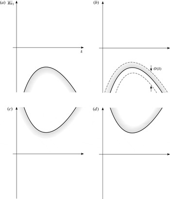The stability diagrams in the $(k,\overline{Ra}_{1})$ -plane for these cases are depicted in figure 2. We note here that case (c) will eventually be shown to not be permissible for physically realistic parameter values, but we leave this case in the discussion for completeness.

Figure 2.

Schematic representation of the neutral-stability curves (solid) and the regions of instability (shaded) for direct modes in the four scenarios: (a) ${\it\Omega}_{1}+\hat{{\it\Omega}}_{1}>0$ , $c_{1}>0$ , $d_{1}<0$ ; (b) ${\it\Omega}_{1}+\hat{{\it\Omega}}_{1}>0$ , $c_{1}<0$ , $d_{1}>0$ ; (c) ${\it\Omega}_{1}+\hat{{\it\Omega}}_{1}<0$ , $c_{1}>0$ , $d_{1}<0$ ; (d) ${\it\Omega}_{1}+\hat{{\it\Omega}}_{1}<0$ , $c_{1}<0$ , $d_{1}>0$ . The stability diagrams for case (a) are qualitatively related to those for case (d) by the sign change $\overline{Ra}_{1}\mapsto -\overline{Ra}_{1}$ , ${\it\Omega}_{1}+\hat{{\it\Omega}}_{1}\mapsto -({\it\Omega}_{1}+\hat{{\it\Omega}}_{1})$ , $c_{1}\mapsto -c_{1}$ and $d_{1}\mapsto -d_{1}$ ; similarly for cases (b) and (c). It should be noted that $c_{1}$ and $d_{1}$ have opposite signs in each case, so that overstability does not arise. In each plot, the stability results from the small- ${\it\delta}$ theory are strictly valid locally in a region of width $O({\it\delta})$ centred on the neutral-stability boundary, as indicated in (b).

The presence of different convective scenarios, and hence the nature of the driving mechanisms, is quite sensitive to the parameters $Le_{j}$ and $\mathscr{C}_{j}$ (through the groups ${\it\Omega}_{1}+\hat{{\it\Omega}}_{1}$ , $c_{1}$ and $d_{1}$ ). To emphasize the sensitivity of the system to $Le_{j}$ and $\mathscr{C}_{j}$ in isolation, we examine the following two parameter regimes: (i) $\mathit{Le}_{1}=\mathit{Le}_{2}$ , which we refer to as a ‘single-solute-diffusive’ regime; (ii) $\mathscr{C}_{1}=\mathscr{C}_{2}$ , which we refer to as a ‘single-solute-rejection’ regime. The parameters $\mathscr{C}_{j}$ measure the effective rates of solute rejection, involving a joint effect of the segregation coefficients $k_{j}$ and compositional ratios $\bar{C}_{j}^{bot}$ . The independent effects of a difference in $k_{j}$ and a difference in $\bar{C}_{j}^{bot}$ are discussed in § 5. For simplicity, we take $\bar{S}=0$ , noting that the limit $\bar{S}\rightarrow 0$ is non-singular. We assume that $0\leqslant {\it\phi}_{0}<1$ , $0<m_{j}<1$ , $\mathit{Le}_{j}>1$ and $\mathscr{C}_{j}\leqslant 0$ throughout.

(i) When $\mathit{Le}_{1}=\mathit{Le}_{2}\equiv \mathit{Le}$ , scenario (a) occurs if

(4.12) $$\begin{eqnarray}\mathscr{C}_{2}/\mathscr{C}_{1}>1.\end{eqnarray}$$

Next, scenario (b) occurs if either of the following two sets of criteria is satisfied:

(4.13a ) $$\begin{eqnarray}\displaystyle & \displaystyle 1-\frac{1-{\it\phi}_{0}}{m_{2}\mathit{Le}}<\frac{\mathscr{C}_{2}}{\mathscr{C}_{1}}<1-\frac{1-{\it\phi}_{0}}{m_{2}\mathit{Le}^{2}}\quad \text{for }\mathit{Le}\geqslant \frac{1-{\it\phi}_{0}}{m_{2}}, & \displaystyle\end{eqnarray}$$

(4.13b ) $$\begin{eqnarray}\displaystyle & \displaystyle 0\leqslant \frac{\mathscr{C}_{2}}{\mathscr{C}_{1}}<1-\frac{1-{\it\phi}_{0}}{m_{2}\mathit{Le}^{2}}\quad \text{for }\left(\frac{1-{\it\phi}_{0}}{m_{2}}\right)^{1/2}<\mathit{Le}<\frac{1-{\it\phi}_{0}}{m_{2}}. & \displaystyle\end{eqnarray}$$

Finally, scenario (d) arises if

(4.14) $$\begin{eqnarray}0\leqslant \frac{\mathscr{C}_{2}}{\mathscr{C}_{1}}<1-\frac{1-{\it\phi}_{0}}{m_{2}\mathit{Le}}\quad \text{for }\mathit{Le}>\frac{1-{\it\phi}_{0}}{m_{2}}.\end{eqnarray}$$

It should be noted that scenario (c) does not arise in this regime.

(ii) When $\mathscr{C}_{1}=\mathscr{C}_{2}\equiv \mathscr{C}$ , we find that only scenario (a) can arise provided

(4.15) $$\begin{eqnarray}\mathit{Le}_{1}<\mathit{Le}_{2}<{\textstyle \frac{1}{2}}\left\{\mathit{Le}_{1}+1+[(\mathit{Le}_{1}+1)^{2}+4m_{1}\mathit{Le}_{1}/m_{2}]^{1/2}\right\},\end{eqnarray}$$

independently of $\mathscr{C}$ .

These results will be exploited and physical interpretations discussed after the oscillatory modes have been presented below.

4.2.2. Oscillatory modes

When $\overline{Ra}=\overline{Ra}_{2}=0$ (case 1), the neutrally stable oscillatory modes must satisfy (4.8) and (4.9) with $({\it\sigma}_{I}^{1})^{2}>0$ . Notably, a non-zero solution for ${\it\sigma}_{I}^{1}$ , indicating the presence of an oscillatory instability, depends on a single parameter combination $Q_{1}$ and the wavenumber $k$ . By analysing (4.9) for $n=1$ in the limit of small ${\it\sigma}_{I}^{1}$ , we find that the oscillatory modes occur for $Q_{1}>{\rm\pi}^{2}/[4({\rm\pi}^{2}+k^{2})]$ .

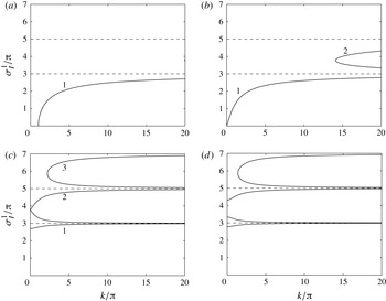
Figure 3 shows the effect of $Q_{1}$ on the solution structure ${\it\sigma}_{I}^{1}$ versus $k$ for $n=1$ , as computed from (4.9). At a fixed $Q_{1}$ , we find that there is a family of disjoint branches, with the associated ${\it\sigma}_{I}^{1}$ lying in the intervals $(0,3{\rm\pi})$ and $((2l+1){\rm\pi},(2l+3){\rm\pi})$ , where $l$ is a positive integer. The branches approach limiting values ${\it\sigma}_{I}^{1}=(2l+1){\rm\pi}$ as $k\rightarrow \infty$ . Thus, many more solution branches occur for increasing values of $k$ ; only the first three, labelled 1–3, are apparent in figure 3. For $Q_{1}<{\textstyle \frac{1}{4}}$ , the lowest branch (mode 1) features a long-wavelength cutoff at $k=k_{\mathit{cutoff}}\equiv {\rm\pi}\left[1/\left(4Q_{1}\right)-1\right]^{1/2}$ , below which the oscillatory instability does not persist (e.g. figure 3 a). For $Q_{1}\geqslant {\textstyle \frac{1}{4}}$ , this solution is present at all wavenumbers, including zero wavenumber (figures 3 b–d). As $Q_{1}$ increases, each of the higher branches (modes 2 and 3) undergoes a breakup at zero wavenumber, forming a decoupled pair of branches; for mode 2 this occurs at $Q_{1}\approx 49.867$ (figure 3 c). Similar behaviour is exhibited by the next higher branches on increasing $Q_{1}$ further.

Figure 3.

Frequency ${\it\sigma}_{I}^{1}$ as a function of wavenumber $k$ for $n=1$ and (a) $Q_{1}={\textstyle \frac{1}{8}}$ , (b) $Q_{1}={\textstyle \frac{1}{4}}$ , (c) $Q_{1}\approx 49.867$ and (d) $Q_{1}=100$ . In each case, there is a family of disjoint solution branches, asymptoting to ${\it\sigma}_{I}^{1}=(2l+1){\it\pi}$ as $k\rightarrow \infty$ (dashed), where $l$ is a positive integer. Many more branches occur for increasing $k$ ; only the first three, labelled 1–3, are shown. The scales in each plot are the same to allow the effect of $Q_{1}$ to be seen more easily. For $Q_{1}<{\textstyle \frac{1}{4}}$ , as in (a), there is a long-wavelength cutoff along the mode-1 branch. In (c), there is a breakup of the mode-2 branch, resulting in a decoupled pair of branches, as apparent in (d). Similar behaviour is exhibited by all the higher solution branches.

When $Q_{1}>0$ , the different stability scenarios can be categorized as follows: (a) ${\it\Omega}_{1}+\hat{{\it\Omega}}_{1}>0$ , $c_{1}>0$ , $d_{1}>0$ ; (b) ${\it\Omega}_{1}+\hat{{\it\Omega}}_{1}>0$ , $c_{1}<0$ , $d_{1}<0$ ; (c) ${\it\Omega}_{1}+\hat{{\it\Omega}}_{1}<0$ , $c_{1}>0$ , $d_{1}>0$ ; (d) ${\it\Omega}_{1}+\hat{{\it\Omega}}_{1}<0$ , $c_{1}<0$ , $d_{1}<0$ . It should be noted that these are the same as the previous cases (a)–(d) for direct modes, except that the sign of $d_{1}$ , and hence $Q_{1}$ , is reversed. Again, we note that case (c) will eventually be shown to not be permissible for physically realistic parameter values, but we leave this case in the discussion for completeness. 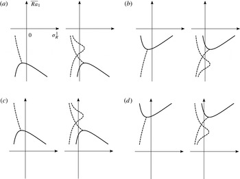The stability diagrams in the $(k,\overline{Ra}_{1})$ -plane for these cases are depicted in figure 4. The corresponding growth rates ${\it\sigma}_{R}^{1}$ as functions of Rayleigh number $\overline{Ra}_{1}$ at fixed $k$ are depicted in figure 5.

Figure 4.

Schematic representation of the neutral-stability curves for the direct mode (solid), the oscillatory modes (dashed), the transition boundary separating the growing direct modes from the growing oscillatory modes (dotted), and the regions of instability (shaded) in the four scenarios: (a) ${\it\Omega}_{1}+\hat{{\it\Omega}}_{1}>0$ , $c_{1}>0$ , $d_{1}>0$ ; (b) ${\it\Omega}_{1}+\hat{{\it\Omega}}_{1}>0$ , $c_{1}<0$ , $d_{1}<0$ ; (c) ${\it\Omega}_{1}+\hat{{\it\Omega}}_{1}<0$ , $c_{1}>0$ , $d_{1}>0$ ; (d) ${\it\Omega}_{1}+\hat{{\it\Omega}}_{1}<0$ , $c_{1}<0$ , $d_{1}<0$ . The stability diagrams for case (a) are qualitatively related to those for case (d) by the sign change $\overline{Ra}_{1}\mapsto -\overline{Ra}_{1}$ , ${\it\Omega}_{1}+\hat{{\it\Omega}}_{1}\mapsto -({\it\Omega}_{1}+\hat{{\it\Omega}}_{1})$ , $c_{1}\mapsto -c_{1}$ and $d_{1}\mapsto -d_{1}$ ; similarly for cases (b) and (c). It should be noted that $c_{1}$ and $d_{1}$ have the same sign in each case, so that oscillatory modes are present for sufficiently large wavenumbers. Only the first three oscillatory branches are shown. As in figure 2, the results are valid only in a local sense (i.e. within an $O({\it\delta})$ neighbourhood of the neutral-stability boundary).

Figure 5.

Growth rate ${\it\sigma}_{R}^{1}$ as a function of Rayleigh number $\overline{Ra}_{1}$ (shown in the ${\it\sigma}_{R}^{1}$ versus $\overline{Ra}_{1}$ plane) for fixed $k$ and $n=1$ . Cases (a–d) correspond to the neutral-stability diagrams portrayed in figures 4(a–d), respectively, with the plots on the left (right) representing cross-sections at $k<k_{\mathit{cutoff}}$ ( $k>k_{\mathit{cutoff}}$ );  $k_{\mathit{cutoff}}$ is the lowest oscillatory mode wavenumber cutoff as identified in the analysis of § 4.2. In each plot, the solid (dashed) curve corresponds to the direct (oscillatory) solution branch; only the first two oscillatory modes are indicated.

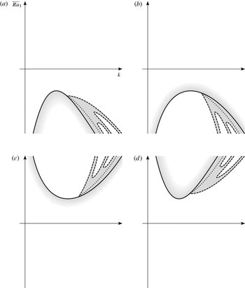
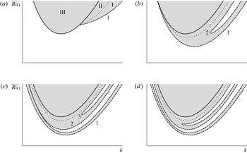
The situation shown in figure 4 is representative but does not illustrate the full range of possible behaviours. In particular, the details vary as $Q_{1}$ varies in accordance with the results of figure 3. Figure 6 depicts the sketches of the neutral-stability curve for the direct mode (solid), the neutral-stability curves for the oscillatory modes (dashed) and the transition boundary between the growing direct modes and the growing oscillatory modes (dotted) for illustrative values of $Q_{1}$ . The results shown correspond to scenario (d) in figure 4; scenarios (a–c) possess similar behaviour. The neutral curves for the oscillatory modes can be associated with the frequency solution branches shown in figure 3. Figure 6(a) shows a case when $Q_{1}<{\textstyle \frac{1}{4}}$ , in which the lowest oscillatory curve (mode 1) terminates on the direct curve at a finite $k$ with an associated ${\it\sigma}_{I}^{1}$ of zero. When $Q_{1}={\textstyle \frac{1}{4}}$ , this termination occurs at $k=0$ (figure 6 b), while for $Q_{1}>{\textstyle \frac{1}{4}}$ the branches do not intersect (figures 6 c,d). A couple of further aspects related to the juxtaposition of the higher oscillatory modes and the direct mode are illustrated in figure 6 for (c) $Q_{1}\approx 49.867$ and (d) $Q_{1}>49.867$ . In (c) the second oscillatory branch (mode 2) splits at $k=0$ , forming a pair of decoupled oscillatory branches, as apparent in (d). The same qualitative results hold also for the higher oscillatory modes. It should be noted also that these modes never intersect the direct mode.

Figure 6.

Sketches of typical neutral-stability curves for the direct mode (solid), the oscillatory modes (dashed) and the transition boundary separating the growing direct modes from the growing oscillatory modes (dotted) in the $(k,\overline{Ra}_{1})$ -plane for representative cases (a) $0<Q_{1}<{\textstyle \frac{1}{4}}$ , (b) $Q_{1}={\textstyle \frac{1}{4}}$ , (c) $Q_{1}\approx 49.867$ and (d) $49.867<Q_{1}<291.766$ . The oscillatory branches are labelled as in figure 3. Each sketch applies to the case $\overline{Ra}=\overline{Ra}_{2}=0$ (case 1), and ${\it\Omega}_{1}+\hat{{\it\Omega}}_{1}<0$ , $c_{1}<0$ and $d_{1}<0$ (scenario d in figure 4). The system is linearly unstable in the shaded region. This region divides, as in (a), into three domains, marked I–III, in which a pair of growing oscillatory modes exists (I), two growing direct modes exist (II) and a single growing direct mode exists (III). As $Q_{1}$ increases, the point at which the mode-1 branch terminates on the direct branch as well as the noses of the higher oscillatory branches (modes 2 and 3) move to smaller wavenumbers (cf. figure 3). In (b) the mode-1 branch terminates on the direct branch at $k=0$ , while in (c) and (d) there is no such termination. In (c) the mode-2 branch splits at $k=0$ to form a decoupled pair of oscillatory branches, as seen in (d).

As was done for the direct modes, we rewrite the inequalities that define the different scenarios in figure 4 in terms of the original parameters. Three parameter regimes are now of particular interest. Two of these regimes are the same as those discussed for direct modes (regimes (i) and (ii)). Additionally, we examine a more general case when both the double-solute-diffusive and double-solute-rejection effects are present ( $\mathit{Le}_{1}\neq \mathit{Le}_{2}$ and $\mathscr{C}_{1}\neq \mathscr{C}_{2}$ , regime (iii) below).

(i) When $\mathit{Le}_{1}=\mathit{Le}_{2}\equiv \mathit{Le}$ , we find that only scenario (a) can arise, provided either of the following two sets of criteria is satisfied:

(4.16a ) $$\begin{eqnarray}\displaystyle & \displaystyle 1-\frac{1-{\it\phi}_{0}}{m_{2}\mathit{Le}^{2}}<\frac{\mathscr{C}_{2}}{\mathscr{C}_{1}}<1\quad \text{for }\mathit{Le}\geqslant \left(\frac{1-{\it\phi}_{0}}{m_{2}}\right)^{1/2}, & \displaystyle\end{eqnarray}$$

(4.16b ) $$\begin{eqnarray}\displaystyle & \displaystyle \frac{\mathscr{C}_{2}}{\mathscr{C}_{1}}\geqslant 0\quad \text{for }\mathit{Le}<\left(\frac{1-{\it\phi}_{0}}{m_{2}}\right)^{1/2}. & \displaystyle\end{eqnarray}$$

(ii) When $\mathscr{C}_{1}=\mathscr{C}_{2}\equiv \mathscr{C}$ , scenario (a) requires

(4.17) $$\begin{eqnarray}\mathit{Le}_{2}<\mathit{Le}_{1},\end{eqnarray}$$

while scenario (b) occurs if

(4.18) $$\begin{eqnarray}\mathit{Le}_{2}>{\textstyle \frac{1}{2}}\left\{\mathit{Le}_{1}+1+[(\mathit{Le}_{1}+1)^{2}+4m_{1}\mathit{Le}_{1}/m_{2}]^{1/2}\right\}.\end{eqnarray}$$

It should be noted that these criteria are independent of $\mathscr{C}$ . An inspection shows that scenarios (c) and (d) do not arise in this regime.

(iii) We now restore both the double-solute-diffusive ( $\mathit{Le}_{1}\neq \mathit{Le}_{2}$ ) and double-solute-rejection ( $\mathscr{C}_{1}\neq \mathscr{C}_{2}$ ) effects. The question we are asking is whether a combined action of these effects can give rise to scenario (d), particularly to an oscillatory instability when $\overline{Ra}_{1}>0$ . A case that appears to enjoy a particular simplicity has ${\it\phi}_{0}=0$ , in which the scenario of figure 4(d) arises if

(4.19) $$\begin{eqnarray}\frac{\mathit{Le}_{1}}{\mathit{Le}_{2}}<\frac{\mathscr{C}_{2}}{\mathscr{C}_{1}}<1-\frac{1}{m_{2}\mathit{Le}_{2}}\quad \text{for }\mathit{Le}_{2}>\frac{1}{m_{2}}.\end{eqnarray}$$

4.2.3. Regime diagrams

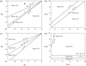
A simple representation of the regions in parameter space, where different convective scenarios are possible, is shown in figure 7. Figure 7(a) shows the results in the ( $\mathscr{C}_{1},\mathscr{C}_{2}$ )-plane for the case of equal Lewis numbers (single-solute-diffusive regime). Figure 7(b) shows the results in the ( $Le_{1},Le_{2}$ )-plane for the case of equal compositional ratios (single-solute-rejection regime). These plots are also extended to more general situations of unequal Lewis numbers (figure 7 c) and unequal compositional ratios (figure 7 d). The transition boundaries between different convective scenarios correspond to the points at which any of the parameter combinations ${\it\Omega}_{1}+\hat{{\it\Omega}}_{1}$ , $c_{1}$ and $d_{1}$ vanishes. It should be noticed that these plots capture all the scenarios that can be found in figures 2 and 4, except for scenario (c). Detailed analysis shows that the latter scenario does not arise for any allowed parameter values. The reduced parameter regimes examined are thus exhaustive. The description may be further generalized to include the effects of latent-heat release, with some implications discussed in § 5.

Figure 7.

Regime diagrams. The regions of different convective scenarios, as identified in figures 2 and 4, are indicated. Plots (a) and (c) show the results in the $(\mathscr{C}_{1},\mathscr{C}_{2})$ -plane, with equal Lewis numbers ( $\mathit{Le}_{1}=\mathit{Le}_{2}=5$ ) in (a) and unequal ones ( $\mathit{Le}_{1}=5$ , $\mathit{Le}_{2}=10$ ) in (c). Plots (b) and (d) show the results in the $(\mathit{Le}_{1},\mathit{Le}_{2})$ -plane, with equal compositional ratios ( $\mathscr{C}_{1}=\mathscr{C}_{2}\equiv \mathscr{C}$ ) in (b) and unequal ones ( $\mathscr{C}_{1}=-5$ , $\mathscr{C}_{2}=-1$ ) in (d). The results in (b) are independent of the value of $\mathscr{C}$ . The remaining parameters are fixed at $\bar{S}=0$ , $m_{1}=m_{2}={\textstyle \frac{1}{2}}$ and ${\it\phi}_{0}=0$ . The neutral-stability curves, validated numerically, at the points marked ○ and ● in (a) are shown in figures 10(a) and (b).

4.3. Case 3: $\overline{Ra}\neq 0$ , $\overline{Ra}_{1}=0$ , $\overline{Ra}_{2}=0$

In the presence of thermal buoyancy alone, the forms (4.7)–(4.9) are unchanged but $\overline{Ra}_{1}$ , ${\it\Omega}_{1}+\hat{{\it\Omega}}_{1}$ , $c_{1}$ and $d_{1}$ are replaced with $\overline{Ra}$ , ${\it\Omega}+\hat{{\it\Omega}}$ , $c$ and $d$ , respectively, where ${\it\Omega}+\hat{{\it\Omega}}=m_{1}({\it\Omega}_{1}+\hat{{\it\Omega}}_{1})+m_{2}({\it\Omega}_{2}+\hat{{\it\Omega}}_{2})$ , $c=m_{1}c_{1}+m_{2}c_{2}$ and $d=m_{1}d_{1}+m_{2}d_{2}$ , or

(4.20a ) $$\begin{eqnarray}\displaystyle & \displaystyle {\it\Omega}+\hat{{\it\Omega}}=\frac{\left(1-{\it\phi}_{0}\right)\left[m_{1}\mathit{Le}_{1}\mathscr{C}_{1}+m_{2}\mathit{Le}_{2}\mathscr{C}_{2}-\left(m_{1}\mathit{Le}_{1}+m_{2}\mathit{Le}_{2}\right)\bar{S}\right]}{m_{1}\mathit{Le}_{1}\mathscr{C}_{1}+m_{2}\mathit{Le}_{2}\mathscr{C}_{2}-\left(1-{\it\phi}_{0}\right)\bar{S}}, & \displaystyle\end{eqnarray}$$

(4.20b ) $$\begin{eqnarray}\displaystyle & \displaystyle c=\frac{\left(m_{1}\mathit{Le}_{1}\mathscr{C}_{1}+m_{2}\mathit{Le}_{2}\mathscr{C}_{2}\right)\!({\it\Omega}+\!\hat{{\it\Omega}})\!-\![m_{1}\mathit{Le}_{1}({\it\Omega}_{1}+\hat{{\it\Omega}}_{1})+m_{2}\mathit{Le}_{2}({\it\Omega}_{2}+\hat{{\it\Omega}}_{2})]\!\left(1\!-{\it\phi}_{0}\right)\bar{S}}{\left(1-{\it\phi}_{0}\right)\left[m_{1}\mathit{Le}_{1}\mathscr{C}_{1}+m_{2}\mathit{Le}_{2}\mathscr{C}_{2}-\left(1-{\it\phi}_{0}\right)\bar{S}\right]}, & \displaystyle \nonumber\\ \displaystyle & & \displaystyle\end{eqnarray}$$

(4.20c ) $$\begin{eqnarray}\displaystyle & \displaystyle d=-\frac{\bar{S}\left[m_{1}\mathit{Le}_{1}+m_{2}\mathit{Le}_{2}-\left(1-{\it\phi}_{0}\right)\right]}{\left[m_{1}\mathit{Le}_{1}\mathscr{C}_{1}+m_{2}\mathit{Le}_{2}\mathscr{C}_{2}-\left(1-{\it\phi}_{0}\right)\bar{S}\right]^{2}}. & \displaystyle\end{eqnarray}$$

$\bar{S}>0$

${\it\Omega}+\hat{{\it\Omega}}$

$d$

$c$

$c>0$

$\overline{Ra}<0$

$c<0$

$\overline{Ra}<0$

$\mathit{Le}_{j}$

$\mathit{Le}_{1}\gg \mathit{Le}_{2}\gg 1$

$c\sim m_{2}\bar{S}\left(\mathscr{C}_{1}-\mathscr{C}_{2}\right)\mathit{Le}_{2}/\left(m_{1}\mathscr{C}_{1}^{2}\right)$

$\mathit{Le}_{2}\gg \mathit{Le}_{1}\gg 1$

However, for the liquid that descends along the liquidus surface upon cooling ( ${\rm\Delta}T^{\ast }>0$ ), both alternatives described above would require increase of the liquid density with increasing temperature ( ${\it\alpha}^{\ast }<0$ ), which is not the usual liquid behaviour.