1 Introduction
In the years since Turing’s pioneering work in morphogenesis (Turing Reference Turing1952), there have been numerous extensions to this basic reaction–diffusion patterning mechanism (Murray Reference Murray2001). One extension is to consider the influence of advection on reaction–diffusion systems, whereby the interacting chemicals are transported along by some process. Resulting reaction–diffusion–advection models have been studied from many different perspectives with a variety of forms of advection. Such models are commonly used to model patterning processes when advection is present for myriad applications, ranging from cell aggregation due to phyllotaxis (Bernasconi & Boissonade Reference Bernasconi and Boissonade1997) to patterning of populations due to directed motion (Grindrod Reference Grindrod1988; Sherratt Reference Sherratt2011; Kurowski et al. Reference Kurowski, Krause, Mizuguchi, Grindrod and Van Gorder2017). Various types of active transport of, e.g. cells, are possible that give rise to advection terms in the governing equations for a population. If the advection is due to the gradients of a function of some given chemical field, then this can model chemotaxis (Hillen & Painter Reference Hillen and Painter2009; Horstmann Reference Horstmann2011). Other forms of cell movement include rheotaxis in the presence of flow (Marcos et al. Reference Fu, Powers and Stocker2012), phyllotaxis in the presence of light (Jönsson et al. Reference Jönsson, Heisler, Shapiro, Meyerowitz and Mjolsness2006; Smith et al. Reference Smith, Guyomarc’h, Mandel, Reinhardt, Kuhlemeier and Prusinkiewicz2006) or magnetotaxis in the presence of an external electromagnetic field (Faivre & Schuler Reference Faivre and Schuler2008). We remark that the morphogens in reaction–diffusion systems are typically thought of as single molecules, such as the proteins Nodal and Lefty (Müller et al. Reference Müller, Rogers, Jordan, Lee, Robson, Ramanathan and Schier2012), but can correspond to other structures, such as cells in different morphological states, or other developmentally important factors (Kondo & Miura Reference Kondo and Miura2010). Here we will be agnostic to the specific nature of the morphogens, and simply consider systems that can be modelled via reaction, diffusion and advection.
Advection of a substance which regulates active tension was incorporated into a two-phase model of the cytoplasm which accounts for the spatio-temporal dynamics of the cytoskeleton and the cytosol by Radszuweit et al. (Reference Radszuweit, Alonso, Engel and Bär2013); more generally, advection due to active stress up regulation by an activator was studied by Bois, Jülicher & Grill (Reference Bois, Jülicher and Grill2011) in the context of patterning in active fluids. Nakagaki, Yamada & Ito (Reference Nakagaki, Yamada and Ito1999) study spatio-temporal patterns of rhythmic contraction within Physarum polycephalumis under the assumption that the chemical oscillator regulates the rhythmic contraction and interacts spatially via diffusion and advection of protoplasm. Their inclusion of an advection effect reproduces certain experimentally observed phenomena such as fluctuation of the contraction wave. A similar analysis was carried out for a reaction–diffusion–advection model of Physarum plasmodium by Yamada, Nakagaki & Ito (Reference Yamada, Nakagaki and Ito1999). Fluid mechanical forces, as well as transport phenomena, have been implicated in several developmental processes (Cartwright, Piro & Tuval Reference Cartwright, Piro and Tuval2009).
Nonlinear advection has been shown to introduce oscillatory instabilities in reaction–convection–diffusion systems as well (Marlow, Sasaki & Vasquez Reference Marlow, Sasaki and Vasquez1997; McGraw & Menzinger Reference McGraw and Menzinger2003). Novel mechanisms and patterns have also been explored experimentally (Rovinsky & Menzinger Reference Rovinsky and Menzinger1993; Nugent, Quarles & Solomon Reference Nugent, Quarles and Solomon2004; Míguez, Satnoianu & Muñuzuri Reference Míguez, Satnoianu and Muñuzuri2006b ) and travelling wave analyses have been carried out (Flach, Schnell & Norbury Reference Flach, Schnell and Norbury2007). Such flow-distributed oscillation routes to spatial pattern formation were experimentally verified in the Beluosov–Zhabotinsky reaction (Kærn & Menzinger Reference Kærn and Menzinger1999, Reference Kærn and Menzinger2000, Reference Kærn and Menzinger2002). In addition to fluid flows with chemical species, we also note that advection of chemical species may be attained through the use of electric fields (Carballido-Landeira, Taboada & Muñuzuri Reference Carballido-Landeira, Taboada and Muñuzuri2012; Dähmlow & Müller Reference Dähmlow and Müller2015; Dähmlow, Luengviriya & Müller Reference Dähmlow, Luengviriya and Müller2015). Reaction–diffusion–advection models have been used to explain chemical–mechanical coupling in particular organisms, such as the rhythmic contraction of the plasmodium of Physarum polycephalum (Nakagaki et al. Reference Nakagaki, Yamada and Ito1999). More complicated reaction–diffusion–advection models have seen recent application to pattern formation of Dictyostelium discoideum (Eckstein et al. Reference Eckstein, Vidal-Henriquez, Bae, Zykov, Bodenschatz and Gholami2018).
Phase differences in reaction–diffusion–advection systems were studied and applied to morphogenesis by Perumpanani, Sherratt & Maini (Reference Perumpanani, Sherratt and Maini1995), with the difference of two constant advection parameters highlighted as critical to the linearized dynamics and resulting diffusion-driven instabilities. Satnoianu & Menzinger (Reference Satnoianu and Menzinger2002) investigated reactive flows as a way of introducing inexact phase differences within Turing patterns, while Andresén et al. (Reference Andresén, Bache, Mosekilde, Dewel and Borckmanns1999) used advection to find Turing patterns with equal diffusion coefficients that would not be possible in the absence of advection. In addition to the Turing instability, such reaction–diffusion–advection systems are known to admit wave instabilities (Rovinsky & Menzinger Reference Rovinsky and Menzinger1992; Flach et al. Reference Flach, Schnell and Norbury2007; Berenstein Reference Berenstein2012a ,Reference Berenstein b ; Ghosh, Paul & Ray Reference Ghosh, Paul and Ray2016), including the case where the inhibitor is immobile (Dawson, Lawniczak & Kapral Reference Dawson, Lawniczak and Kapral1994). Both stationary and travelling patterns may coexist in such reaction–diffusion–advection systems (Satnoianu Reference Satnoianu2003), and wave instabilities manifest in chemical (Riaz, Kar & Ray Reference Riaz, Kar and Ray2004) and ecological (Malchow Reference Malchow1995, Reference Malchow2000) models. Klika, Kozaák & Gaffney (Reference Klika, Kozaák and Gaffney2018) explored the use of advection and combinations of different boundary conditions to relax some of the stringent conditions required for Turing-like instabilities in two-species systems.
In addition to planar dynamics, reaction–diffusion–advection systems have been considered on curved surfaces, such as spheres. Such systems have been used to model the transport of water across the surface of the Earth (Williamson & Rasch Reference Williamson and Rasch1989; Smolarkiewicz & Rasch Reference Smolarkiewicz and Rasch1991), chemical transport due to atmospheric convection (Pudykiewicz Reference Pudykiewicz2006), the transport of microorganisms (Burrows et al. Reference Burrows, Butler, Jöckel, Tost, Kerkweg, Pöschl and Lawrence2009a ,Reference Burrows, Elbert, Lawrence and Pöschl b ) and dust transport in arid environments (Kellogg & Griffin Reference Kellogg and Griffin2006). The birth and death of patterns on the sphere due to source and sink behaviour for a reaction–diffusion–advection system was recently studied by Krause et al. (Reference Krause, Burton, Fadai and Van Gorder2018). In the case of growing geometries, advection-like terms can result from the conversion of the temporally varying spatial problem to one on a static domain (Crampin, Gaffney & Maini Reference Crampin, Gaffney and Maini1999; Plaza et al. Reference Plaza, Sanchez-Garduno, Padilla, Barrio and Maini2004; Barreira, Elliott & Madzvamuse Reference Barreira, Elliott and Madzvamuse2011).
There has been far less work on models which couple chemical systems to spatially heterogeneous advection. A simple tubular reactor with continuous feeding and cooling in which an exothermic Arrhenius reaction, modelled by one equation for the chemical reaction, and another for the flow, was studied in Yochelis & Sheintuch (Reference Yochelis and Sheintuch2009a ); see also Yochelis & Sheintuch (Reference Yochelis and Sheintuch2010). Vasquez (Reference Vasquez2004) studied the instability induced by a shear flow in chemical systems. By coupling the Brusselator system to a Poiseuille flow in a two-dimensional (2-D) rectangular domain, with the flow acting equally on both the activator and inhibitor, Vasquez (Reference Vasquez2004) reason that molecular diffusion in a pipe with a moving fluid can be approximated with an effective diffusion coefficient; since the velocity of the fluid must vary over a given cross-section of the pipe, the local effective diffusion varies spatially. At some locations, the effective diffusivities between the inhibitor and the activator can become greater than unity, even if the diffusion coefficient is less than unity. Vasquez, Meyer & Suedhoff (Reference Vasquez, Meyer and Suedhoff2008) then consider a similar model for a system consisting of two layers moving relative to each other. See also Stucchi & Vasquez (Reference Stucchi and Vasquez2013, Reference Stucchi and Vasquez2014) for similar results on the cubic autocatalytic reaction kinetics, Ayodele, Raabe & Varnik (Reference Ayodele, Raabe and Varnik2015) for results on a two-species Gray–Scott model with advection, Kuptsov, Satnoianu & Daniels (Reference Kuptsov, Satnoianu and Daniels2005) for results on Lengyel–Epstein reaction kinetics for the chlorite-iodide-malonic acid-starch reaction, Liu et al. (Reference Liu, Zhou, Zheng, Zhao, Gao, Pan and Horvaáth2016) for results on the chlorite-trithionate reaction and Ermakova et al. (Reference Ermakova, Shnol, Panteleev, Butylin, Volpert and Ataullakhanov2009) for results on FitzHugh–Nagumo reaction kinetics. There have also been a number of works which have focused on travelling reaction fronts in reaction–diffusion–advection systems under Poiseuille flow (Edwards Reference Edwards2002; Spangler & Edwards Reference Spangler and Edwards2003; Koptyug, Zhivonitko & Sagdeev Reference Koptyug, Zhivonitko and Sagdeev2008; Vasquez & Coroian Reference Vasquez and Coroian2010). The modification of wave fronts in the Kuramoto–Sivashinsky equation due to a Couette flow was considered in Vilela & Vasquez (Reference Vilela and Vasquez2014). Couette flow in a rotating pipe was used to advect single and double-species reaction–diffusion systems in Balinsky & Pismen (Reference Balinsky and Pismen1998), and the influence of this advection on Turing patterns was explicitly discussed.
More theoretically, Straube & Pikovsky (Reference Straube and Pikovsky2011) employ an approach based on Lyapunov–Bloch exponents in order to study pattern formation in reaction–diffusion–advection systems with advection functions which are periodic in space and vary in time. Rickett et al. (Reference Rickett, Penfold, Blyth, Purvis and Cooker2015) consider a two-layer fluid model with chemical species, with a planar Poiseuille flow driven by an external pressure gradient. This flow is seen to enhance growth rates of instabilities, while stable decay is suppressed with increasing base flow speed. Boundary-driven oscillations in reaction–diffusion–advection systems were studied by Vidal-Henriquez et al. (Reference Vidal-Henriquez, Zykov, Bodenschatz and Gholami2017). In many of the aforementioned studies, the ratio of diffusivities is usually taken to unity, as the goal is to study the emergence of patterning due to the advection. In contrast, we shall primarily be interested in situations where the advection modifies existing diffusion-driven patterns emergent without the presence of advection, as these will correspond to canonical Turing patterns.
Control or modification of patterns through spatially uniform constant advection has been considered, with some results suggesting that the advection can modify the robustness of patterns (Satnoianu, Maini & Menzinger Reference Satnoianu, Maini and Menzinger2001; Míguez, Izús & Muñuzuri Reference Míguez, Izús and Muñuzuri2006a ; Yochelis & Sheintuch Reference Yochelis and Sheintuch2009b ). Wei & Winter (Reference Wei and Winter2012) consider the role that advection plays in the dynamics of spike solutions arising under Schnakenberg kinetics. The persistence and robustness of vegetation on slopes were studied by considering striped patterns under a reaction–diffusion–advection model by Siero et al. (Reference Siero, Doelman, Eppinga, Rademacher, Rietkerk and Siteur2015). The rate of advection may modify the pattern formed, with spotted patterns for zero advection becoming travelling spots for small advection under the reaction–diffusion–advection two-dimensional Brusselator model with uniform constant and equal advection studied by Hu, Li & Li (Reference Hu, Li and Li2009). For larger advection, the travelling spots observed by Hu et al. (Reference Hu, Li and Li2009) degenerate into striped patterns. Such travelling patterns have been seen for small advection in other models (Zhou et al. Reference Zhou, Wang, Li and Jin2009), and appear to maintain fidelity for small enough advection. Reaction–diffusion–advection models have also been proposed for spatially localizing treadmilling aggregates of molecular motors (Yochelis, Bar-On & Gov Reference Yochelis, Bar-On and Gov2016). Kim & Lin (Reference Kim and Lin2007) propose an anisotropy embedding in order to expand the space of possible patterns emergent from certain reaction–diffusion–advection systems. Optimal control of a reaction–diffusion–advection form of the FitzHugh–Nagumo equations, with two-dimensional Poiseuille flow, has been considered recently by Uzunca et al. (Reference Uzunca, Küçükseyhan, Yücel and Karasözen2017). Regarding applications, Ledesma-Durán et al. (Reference Ledesma-Durán, Juárez-Valencia, Morales-Malacara and Santamaría-Holek2017) study skin patterns on Pseudoplatystoma fishes and hypothesize that a traveling chemical wave originates the disordered motifs of the pattern and that the advection mechanism later aligns the pattern in specific directions resulting in actually observed striped patterns. Other applications relate to the formation of structures due to the proper combination of patterning and flow properties, with recent work involving the fabrication of intricate three-dimensional (3-D) structures useful in water purification (Tan et al. Reference Tan, Chen, Peng, Zhang and Gao2018).
There has been a good deal of work on flows within unbounded domains, or on manifolds which are compact yet have no boundary. We shall be interested in the case where the flow is confined in some way, such as within a pipe. We shall consider two chemical species embedded within a finite domain, including a 2-D rectangular channel, a 3-D rectangular duct and a 3-D cylindrical pipe. We consider a Poiseuille flow which is driven by a pressure differential between two ends of the domain, as well as uniform flows in order to demonstrate the role of geometry, and to make analytical progress. Numerical simulations are then used to more accurately resolve the patterns which develop in these flows, with our observations suggesting a strong dependence of patterning on both the geometry of the vessel as well as on the form of advection considered. Finally we also numerically explore geometries with substantial boundary curvature, in order to understand flows when the fluid velocity is not confined to be unidirectional.
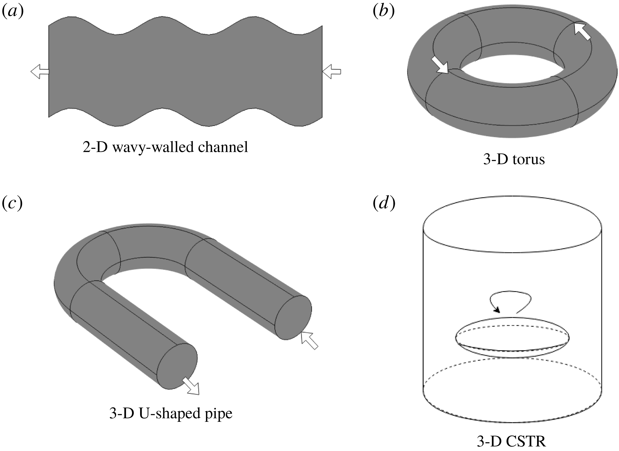
The remainder of the paper is organized as follows. In § 2, we outline the general flow problem, as well as reductions to specific vessel geometries under steady laminar flow. We non-dimensionalize the models and discuss respective time scales in each case. In § 3 we analytically study the linear instability analysis for a general heterogeneous advection problem, and then for the three specific vessel geometries listed above (under spatially averaged advection). For each case, the geometry is shown to play a role in the selection of unstable eigenmodes. Furthermore, we show that the generic instability is that of an oscillatory or wave Turing instability, suggesting that rather than static spatial patterns, spatio-temporal patterns should be expected as the generic behaviour. In § 4, we consider numerical simulations for the three sample vessel geometries, in order to resolve which of the patterns suggested by the analysis of § 3 actually develop. We also discuss the manner in which advection changes the Turing space, with differential advection leading to a wider variety of possible spatial or spatio-temporal patterns that would be found in the absence of advection. In § 5, we consider similar simulations, only for the case of Stokes flow computed numerically in complex curved geometries, in order to ascertain the roles that lateral advection and curvature may play in pattern formation for biological or chemical systems. These examples consist of a wavy-walled channel, a torus, a U-shaped pipe and a simple model of a continuous stirred-tank reactor (CSTR). We summarize and discuss our results in § 6.
2 Coupling of reaction–diffusion models to Stokes flow
A general model for a reaction–diffusion–advection system, with advection due to a fluid flow governed by incompressible Navier–Stokes, is given by
 $$\begin{eqnarray}\displaystyle & \displaystyle \frac{\unicode[STIX]{x2202}u}{\unicode[STIX]{x2202}\tilde{t}}=\unicode[STIX]{x1D6FE}f(u,v)+\tilde{\unicode[STIX]{x1D6FF}}_{u}\unicode[STIX]{x1D6FB}^{2}u-\unicode[STIX]{x1D70E}_{u}\boldsymbol{A}\boldsymbol{\cdot }\unicode[STIX]{x1D735}u, & \displaystyle\end{eqnarray}$$
 $$\begin{eqnarray}\displaystyle & \displaystyle \frac{\unicode[STIX]{x2202}v}{\unicode[STIX]{x2202}\tilde{t}}=\unicode[STIX]{x1D6FE}g(u,v)+\tilde{\unicode[STIX]{x1D6FF}}_{v}\unicode[STIX]{x1D6FB}^{2}v-\unicode[STIX]{x1D70E}_{v}\boldsymbol{A}\boldsymbol{\cdot }\unicode[STIX]{x1D735}v, & \displaystyle\end{eqnarray}$$
 $$\begin{eqnarray}\displaystyle & \displaystyle \unicode[STIX]{x1D735}\boldsymbol{\cdot }\boldsymbol{A}=0, & \displaystyle\end{eqnarray}$$
 $$\begin{eqnarray}\displaystyle & \displaystyle \frac{\unicode[STIX]{x2202}\boldsymbol{A}}{\unicode[STIX]{x2202}\tilde{t}}+(\boldsymbol{A}\boldsymbol{\cdot }\unicode[STIX]{x1D735})\boldsymbol{A}=\unicode[STIX]{x1D708}\unicode[STIX]{x1D6FB}^{2}\boldsymbol{A}-\unicode[STIX]{x1D735}p, & \displaystyle\end{eqnarray}$$
 $$\begin{eqnarray}\displaystyle & \displaystyle \boldsymbol{A}(\tilde{\boldsymbol{x}},t=0)=\boldsymbol{A}_{0}(\tilde{\boldsymbol{x}}), & \displaystyle\end{eqnarray}$$
where
 $u$
and
 $v$
are the chemical species or morphogens and
 $\boldsymbol{A}$
is the advecting flow (while often thought of as a fluid, this could also involve other forces such as an electromagnetic field, in which case the field equations would change). The functions
 $f$
and
 $g$
are the reaction kinetics,
 $\unicode[STIX]{x1D6FE}$
is a parameter which scales the reaction rates,
 $\tilde{\unicode[STIX]{x1D6FF}}_{u}$
and
 $\tilde{\unicode[STIX]{x1D6FF}}_{v}$
are Fickian diffusion parameters,
 $\unicode[STIX]{x1D70E}_{u}$
and
 $\unicode[STIX]{x1D70E}_{v}$
are parameters which couple the morphogens to the flow,
 $\unicode[STIX]{x1D708}$
is the fluid viscosity and
 $p$
is the pressure.
The spatial variable
 $\tilde{\boldsymbol{x}}$
will be dictated by the problem geometry. In a 2-D rectangular channel, we have
 $\tilde{\boldsymbol{x}}=(\tilde{x},{\tilde{y}})$
, while in a 3-D rectangular duct,
 $\tilde{\boldsymbol{x}}=(\tilde{x},{\tilde{y}},\tilde{z})$
and in a 3-D cylindrical pipe,
 $\tilde{\boldsymbol{x}}=(\tilde{r},\tilde{\unicode[STIX]{x1D703}},\tilde{x})$
. More generally, for our theoretical analysis, we shall most often consider a coordinate frame
 $\tilde{\boldsymbol{x}}=(\tilde{x},\tilde{\boldsymbol{y}})$
, where the domain does not vary in the
 $\tilde{x}$
direction, which is also the direction of the flow, while
 $\tilde{\boldsymbol{y}}$
denotes the variables in the cross-section (
 ${\tilde{y}}$
for a 2-D channel flow,
 ${\tilde{y}},\tilde{z}$
for a 3-D duct flow,
 $\tilde{r},\tilde{\unicode[STIX]{x1D703}}$
for a 3-D pipe flow). Then, we take the problem domain
 $\unicode[STIX]{x1D6FA}=[0,L]\times \unicode[STIX]{x1D6FA}^{\prime }$
, where
 $\unicode[STIX]{x1D6FA}^{\prime }$
denotes the cross-section, which we assume is simply connected. We shall consider steady laminar flow via Stokes flow, rather than the full Navier–Stokes equations, in which case (2.4) reduces to the Stokes flow problem
 $$\begin{eqnarray}\unicode[STIX]{x1D6FB}^{2}\boldsymbol{A}=\frac{1}{\unicode[STIX]{x1D708}}\unicode[STIX]{x1D735}p.\end{eqnarray}$$
This is sensible, as creeping flow is the proper regime for advection of the chemical species to balance diffusion.
We shall assume that the flow is driven by a constant pressure gradient in the
 $\tilde{x}$
direction, say
 $\unicode[STIX]{x1D735}p=\unicode[STIX]{x2202}p/\unicode[STIX]{x2202}x=P_{\triangle }$
. Then, the velocity profile takes the form
 $$\begin{eqnarray}\boldsymbol{A}=\left(\frac{P_{\triangle }}{\unicode[STIX]{x1D708}}A_{\tilde{x}}(\tilde{\boldsymbol{y}}),\mathbf{0}\right),\end{eqnarray}$$
where
 $A_{\tilde{x}}(\tilde{\boldsymbol{y}})$
is a scalar function defined on each cross-section
 $\unicode[STIX]{x1D6FA}^{\prime }$
as the solution to Poisson’s equation
 $$\begin{eqnarray}\unicode[STIX]{x1D6FB}_{\tilde{\boldsymbol{y}}}^{2}A_{\tilde{x}}=1,\quad \text{in }\unicode[STIX]{x1D6FA}^{\prime },\quad \boldsymbol{n}\boldsymbol{\cdot }\unicode[STIX]{x1D735}_{\tilde{\boldsymbol{ y}}}A_{\tilde{x}}=0,\quad \text{on }\unicode[STIX]{x2202}\unicode[STIX]{x1D6FA}^{\prime }.\end{eqnarray}$$
2.1 Dimensionless model
We scale time with the reaction rate,
 $\tilde{t}=\unicode[STIX]{x1D6FE}^{-1}t$
, where
 $t$
is dimensionless. We scale spatial variables as
 $\tilde{x}=Lx$
and
 $\tilde{\boldsymbol{y}}=H\boldsymbol{y}$
, where
 $L$
and
 $H$
are characteristic length scales, while
 $x$
and
 $\boldsymbol{y}$
are dimensionless spatial coordinates. We then have
 $x\in [0,1]$
, while
 $H$
is selected so that
 $|\boldsymbol{y}|=O(1)$
. The dimensionless forms of (2.1)–(2.2) are then given by
 $$\begin{eqnarray}\displaystyle & \displaystyle \frac{\unicode[STIX]{x2202}u}{\unicode[STIX]{x2202}t}=f(u,v)+\unicode[STIX]{x1D6FF}_{u}\unicode[STIX]{x1D6FB}_{\boldsymbol{y}}^{2}u+\unicode[STIX]{x1D6FF}_{u}\unicode[STIX]{x1D6FC}^{2}\frac{\unicode[STIX]{x2202}^{2}u}{\unicode[STIX]{x2202}x^{2}}-\unicode[STIX]{x1D6FD}_{u}A(\boldsymbol{y})\frac{\unicode[STIX]{x2202}u}{\unicode[STIX]{x2202}x}, & \displaystyle\end{eqnarray}$$
 $$\begin{eqnarray}\displaystyle & \displaystyle \frac{\unicode[STIX]{x2202}v}{\unicode[STIX]{x2202}t}=g(u,v)+\unicode[STIX]{x1D6FF}_{v}\unicode[STIX]{x1D6FB}_{\boldsymbol{y}}^{2}v+\unicode[STIX]{x1D6FF}_{v}\unicode[STIX]{x1D6FC}^{2}\frac{\unicode[STIX]{x2202}^{2}v}{\unicode[STIX]{x2202}x^{2}}-\unicode[STIX]{x1D6FD}_{v}A(\boldsymbol{y})\frac{\unicode[STIX]{x2202}v}{\unicode[STIX]{x2202}x}, & \displaystyle\end{eqnarray}$$
where
 $\unicode[STIX]{x1D6FB}_{\boldsymbol{y}}^{2}$
denotes the Laplacian in those coordinates orthogonal to the flow direction within the cross-section
 $\unicode[STIX]{x1D6FA}^{\prime }$
. The dimensionless diffusion parameters are
 $\unicode[STIX]{x1D6FF}_{u}=\tilde{\unicode[STIX]{x1D6FF}}_{u}/(\unicode[STIX]{x1D6FE}H^{2})$
and
 $\unicode[STIX]{x1D6FF}_{v}=\tilde{\unicode[STIX]{x1D6FF}}_{v}/(\unicode[STIX]{x1D6FE}H^{2})$
, whereas the dimensionless advection parameters are
 $$\begin{eqnarray}\unicode[STIX]{x1D6FD}_{u}={\displaystyle \frac{\unicode[STIX]{x1D70E}_{u}H^{2}P_{\triangle }|A_{avg}|}{\unicode[STIX]{x1D708}\unicode[STIX]{x1D6FE}L}}\quad \text{and}\quad \unicode[STIX]{x1D6FD}_{u}={\displaystyle \frac{\unicode[STIX]{x1D70E}_{v}H^{2}P_{\triangle }|A_{avg}|}{\unicode[STIX]{x1D708}\unicode[STIX]{x1D6FE}L}}.\end{eqnarray}$$
The function
 $A(\boldsymbol{y})$
is a normalized solution to (2.8), so that
 $A_{\tilde{x}}(\tilde{\boldsymbol{y}})=H^{2}A_{avg}A(\boldsymbol{y})$
, where
 $A_{avg}$
denotes the averaged value of the flow within the cross-section, and
 $\int _{\unicode[STIX]{x1D6FA}^{\prime }}A(\boldsymbol{y})\,\text{d}\boldsymbol{y}=1$
, so that
 $A(\boldsymbol{y})$
holds the spatial structure of the flow. Finally,
 $\unicode[STIX]{x1D6FC}=H/L$
denotes the aspect ratio of the domain.
We keep the parameter restrictions and hence analysis as general as possible, so that our results are applicable to a wide variety of reactions and flow regimes. Having selected the reaction time scale, we consider
 $0<\unicode[STIX]{x1D6FF}_{u,v}\ll 1$
, since the diffusion time scale is small relative to the reaction time scale. As advection of the chemical with the flow can be controlled via a pressure gradient, one may consider either
 $|\unicode[STIX]{x1D6FD}_{u,v}|\ll 1$
or
 $|\unicode[STIX]{x1D6FD}_{u,v}|=O(1)$
. For
 $|\unicode[STIX]{x1D6FD}_{u,v}|\gg 1$
, there is no longer a balance between reaction kinetics and the advection, and in this case advection acts on such a fast time scale that it is not locally noticed by the reactions. Furthermore, for very fast flows, we would more properly have to consider full Navier–Stokes, rather than Stokes, flows. As such, we restrict our attention to
 $-1\leqslant \unicode[STIX]{x1D6FD}_{u,v}\leqslant 1$
, noting that
 $\unicode[STIX]{x1D6FD}_{u,v}$
can be positive or negative, depending on the direction of the pressure gradient, as well as on the coupling parameters
 $\unicode[STIX]{x1D70E}_{u,v}$
. For bounded domains which are long enough to allow for patterns to develop and persist, one would require
 $\unicode[STIX]{x1D6FC}\ll 1$
. However, when considering periodic domains, we take
 $\unicode[STIX]{x1D6FC}=O(1)$
, and can in that setting view
 $\unicode[STIX]{x1D6FC}$
as a local aspect ratio.
In parameter regimes we consider, the convective and diffusive Damköhler numbers satisfy
 $Da\ll 1$
and
 $Da_{\text{II}}\ll 1$
, as the reaction rate is large relative to convective and diffusive effects. This is the sensible limit for spatial patterning. Otherwise, the reactions will occur too slowly for there to be enough local reaction to allow for spatial patterning, since the chemicals will diffuse uniformly before reaction can occur. On the other hand, the Péclet number is not restricted in such a manner since both diffusion and advection may be independently small or large (albeit both must be small relative to the reaction rate), and broadly both our theoretical results and simulations hold for the full range of Péclet numbers. We will, however, show that different Péclet numbers can select different eigenmodes, and hence qualitatively different patterns will emerge.
2.2 Reaction kinetics
While we will consider a general linear stability analysis for arbitrary reaction kinetics, we choose a specific example for numerical simulations. We will confine our attention to simulations of the Schnakenberg kinetics (Schnakenberg Reference Schnakenberg1979), also known as the activator-depleted model, which can be described by the (non-dimensional) functions
 $$\begin{eqnarray}\displaystyle & \displaystyle f(u,v)=a-u+u^{2}v, & \displaystyle\end{eqnarray}$$
 $$\begin{eqnarray}\displaystyle & \displaystyle g(u,v)=b-u^{2}v, & \displaystyle\end{eqnarray}$$
 $a>0$
and
 $b>0$
are production rates of the activator and inhibitor, respectively. This model admits the spatially homogeneous steady state given by
 $u^{\ast }=a+b$
and
 $v^{\ast }=b/(a+b)^{2}$
. We choose this model as it can exhibit both spot solutions and stripe (labyrinthine) patterns in two spatial dimensions depending on the cubic terms when written in a normal form (Ermentrout Reference Ermentrout1991). The two-dimensional spot and stripe (labyrinthine) patterns have been shown in a variety of works (Boissonade, Dulos & De Kepper Reference Boissonade, Dulos and De Kepper1995; Shoji, Iwasa & Kondo Reference Shoji, Iwasa and Kondo2003), and this makes the Schnakenberg kinetics an attractive choice, since the behaviour in the absence of advection is well understood. In three dimensions, the number of qualitatively distinct patterns becomes quite large (Shoji et al.
Reference Shoji, Yamada, Ueyama and Ohta2007; Dehghan & Abbaszadeh Reference Dehghan and Abbaszadeh2016), although we are unaware of any such classification of such states applicable to this simple system. Instead, we will emphasize the roles of domain shape and curvature, as well as advection, in the selection and stabilization of different patterns.
Note that the reaction kinetics are derived under the assumption that the chemical reactions take place in thermal equilibrium, and with no net heat energy absorbed or released, hence the reaction is neither endothermic nor exothermic. It is possible to consider more complicated/realistic reactions, but even in the case of no fluid flow there is not much literature on this case. Our present results (as well as existing Turing instability results in the purely reaction–diffusion setting) are therefore assumed to correspond with a thermal steady state.
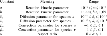
We provide a range of reaction kinetic parameters as well as dimensionless mass transfer parameters in table 1.
Table of dimensionless groups and dimensionless reaction kinetic parameters.

2.3 Turing instability in reaction–diffusion subsystem
We summarize the Turing instability mechanism in reaction–diffusion systems, so that we may later explore how advection will change the instability mechanism and resulting patterns. To this end, we consider the dimensionless model (2.9)–(2.10) in the absence of advection, e.g.
 $\unicode[STIX]{x1D6FD}_{u}=\unicode[STIX]{x1D6FD}_{v}=0$
. Assuming that
 $(u^{\ast },v^{\ast })$
is a spatially homogeneous solution satisfying the algebraic equations
 $f(u^{\ast },v^{\ast })=0$
and
 $g(u^{\ast },v^{\ast })=0$
, we consider a perturbation
 $u=u^{\ast }+\unicode[STIX]{x1D716}\hat{u}$
and
 $v=v^{\ast }+\unicode[STIX]{x1D716}\hat{v}$
, for small
 $0<\unicode[STIX]{x1D716}\ll 1$
. We shall only be interested in spatially homogeneous steady states which are stable under the reaction kinetics, and upon defining
 $f_{u}^{\ast }=(\unicode[STIX]{x2202}f/\unicode[STIX]{x2202}u)(u^{\ast },v^{\ast })$
,
 $f_{v}^{\ast }=(\unicode[STIX]{x2202}f/\unicode[STIX]{x2202}v)(u^{\ast },v^{\ast })$
,
 $g_{u}^{\ast }=(\unicode[STIX]{x2202}g/\unicode[STIX]{x2202}u)(u^{\ast },v^{\ast })$
,
 $g_{v}^{\ast }=(\unicode[STIX]{x2202}g/\unicode[STIX]{x2202}v)(u^{\ast },v^{\ast })$
, we require that the Jacobian matrix of the reaction kinetics has negative trace and positive determinant, i.e.
 $$\begin{eqnarray}f_{u}^{\ast }+g_{v}^{\ast }<0\quad \text{and}\quad f_{u}^{\ast }g_{v}^{\ast }-f_{v}^{\ast }g_{u}^{\ast }>0.\end{eqnarray}$$
From (2.9)–(2.10), the linear perturbations must satisfy the linear system
 $$\begin{eqnarray}\displaystyle & \displaystyle \frac{\unicode[STIX]{x2202}\hat{u} }{\unicode[STIX]{x2202}t}=f_{u}^{\ast }\hat{u} +f_{v}^{\ast }\hat{v}+\unicode[STIX]{x1D6FF}_{u}\unicode[STIX]{x1D6FB}_{\boldsymbol{y}}^{2}\hat{u} +\unicode[STIX]{x1D6FF}_{u}\unicode[STIX]{x1D6FC}^{2}\frac{\unicode[STIX]{x2202}^{2}\hat{u} }{\unicode[STIX]{x2202}x^{2}}, & \displaystyle\end{eqnarray}$$
 $$\begin{eqnarray}\displaystyle & \displaystyle \frac{\unicode[STIX]{x2202}\hat{v}}{\unicode[STIX]{x2202}t}=g_{u}^{\ast }\hat{u} +g_{v}^{\ast }\hat{v}+\unicode[STIX]{x1D6FF}_{v}\unicode[STIX]{x1D6FB}_{\boldsymbol{y}}^{2}\hat{v}+\unicode[STIX]{x1D6FF}_{v}\unicode[STIX]{x1D6FC}^{2}\frac{\unicode[STIX]{x2202}^{2}\hat{v}}{\unicode[STIX]{x2202}x^{2}}. & \displaystyle\end{eqnarray}$$
For a general domain of cross-section
 $\unicode[STIX]{x1D6FA}^{\prime }$
, we assume
 $$\begin{eqnarray}\left(\begin{array}{@{}c@{}}\hat{u} \\ \hat{v}\end{array}\right)=\left(\begin{array}{@{}c@{}}\overline{u}\\ \overline{v}\end{array}\right)\exp (\text{i}kx+\unicode[STIX]{x1D706}t)w(\boldsymbol{y}),\end{eqnarray}$$
where
 $\overline{u}$
and
 $\overline{v}$
are constants,
 $k\in \mathbb{Z}$
,
 $\unicode[STIX]{x1D706}\in \mathbb{C}$
, while
 $w(y)$
is a solution to the eigenvalue problem
 $$\begin{eqnarray}\unicode[STIX]{x1D6FB}_{\boldsymbol{y}}^{2}w=-\unicode[STIX]{x1D71E}w,\quad \text{for }\boldsymbol{y}\in \unicode[STIX]{x1D6FA}^{\prime },\quad \unicode[STIX]{x1D735}_{\boldsymbol{ y}}w\boldsymbol{\cdot }\boldsymbol{n}=0,\quad \text{on }\boldsymbol{y}\in \unicode[STIX]{x2202}\unicode[STIX]{x1D6FA}^{\prime }.\end{eqnarray}$$
Assuming that the cross-section is a simply connected and sufficiently smooth domain, the spectrum is discrete and takes the form
 $0=\unicode[STIX]{x1D71E}_{0}\leqslant \unicode[STIX]{x1D71E}_{1}\leqslant \unicode[STIX]{x1D71E}_{2}\leqslant \cdots \,$
with
 $\unicode[STIX]{x1D71E}_{\ell }\rightarrow \infty$
as the index
 $\ell \rightarrow \infty$
. Note that the precise values of
 $\unicode[STIX]{x1D71E}_{\ell }$
will depend on the form of
 $\unicode[STIX]{x1D6FA}^{\prime }$
. With this, (2.14)–(2.15) reduces to the algebraic system
 $$\begin{eqnarray}\unicode[STIX]{x1D706}\left(\begin{array}{@{}cc@{}}1 & 0\\ 0 & 1\end{array}\right)\left(\begin{array}{@{}c@{}}\overline{u}\\ \overline{v}\end{array}\right)=\left(\begin{array}{@{}cc@{}}f_{u}^{\ast }-\unicode[STIX]{x1D6FF}_{u}(k^{2}\unicode[STIX]{x03C0}^{2}\unicode[STIX]{x1D6FC}^{2}+\unicode[STIX]{x1D71E}_{\ell }) & f_{v}^{\ast }\\ g_{u}^{\ast } & g_{v}^{\ast }-\unicode[STIX]{x1D6FF}_{v}(k^{2}\unicode[STIX]{x03C0}^{2}\unicode[STIX]{x1D6FC}^{2}+\unicode[STIX]{x1D71E}_{\ell })\end{array}\right)\left(\begin{array}{@{}c@{}}\overline{u}\\ \overline{v}\end{array}\right)=J(k,\ell )\left(\begin{array}{@{}c@{}}\overline{u}\\ \overline{v}\end{array}\right).\end{eqnarray}$$
A perturbation of the form (2.16) is linearly unstable provided that one of the corresponding
 $\unicode[STIX]{x1D706}=\unicode[STIX]{x1D706}(k,\ell )$
satisfies
 $\text{Re}(\unicode[STIX]{x1D706}(k,\ell ))>0$
. From the stable reaction kinetics,
 $\text{tr}(J(0,0))<0$
and
 $\det (J(0,0))>0$
. Further, from (2.18), we have
 $\text{tr}(J(k,\ell ))=\text{tr}(J(0,0))-(\unicode[STIX]{x1D6FF}_{u}+\unicode[STIX]{x1D6FF}_{v})(k^{2}\unicode[STIX]{x03C0}^{2}\unicode[STIX]{x1D6FC}^{2}+\unicode[STIX]{x1D71E}_{\ell })<\text{tr}(J(0,0))<0$
. So,
 $\text{Re}(\unicode[STIX]{x1D706}(k,\ell ))>0$
if and only if
 $\det (J(k,\ell ))<0$
for the pair
 $(k,\ell )$
. Yet, when
 $(k,\ell )=(0,0)$
, we have
 $\det (J(0,0))>0$
, and we may also verify that
 $\det (J(k,\ell ))>0$
in the limit
 $k^{2}+\ell ^{2}\rightarrow \infty$
. Therefore, there are at most a bounded set of pairs
 $(k,\ell )$
for which
 $\det (J(k,\ell ))<0$
. Explicitly calculating
 $\det (J(k,\ell ))$
from (2.18), we find that the necessary conditions on the reaction kinetics and diffusion parameters are as follows:
 $$\begin{eqnarray}\unicode[STIX]{x1D6FF}_{u}g_{v}^{\ast }+\unicode[STIX]{x1D6FF}_{v}f_{u}^{\ast }>0\quad \text{and}\quad (\unicode[STIX]{x1D6FF}_{u}g_{v}^{\ast }+\unicode[STIX]{x1D6FF}_{v}f_{u}^{\ast })^{2}-4\unicode[STIX]{x1D6FF}_{u}\unicode[STIX]{x1D6FF}_{v}(f_{u}^{\ast }g_{v}^{\ast }-f_{v}^{\ast }g_{u}^{\ast })>0.\end{eqnarray}$$
Let us define the parameter combinations
 $$\begin{eqnarray}{\mathcal{K}}_{\pm }=\frac{\unicode[STIX]{x1D6FF}_{u}g_{v}^{\ast }+\unicode[STIX]{x1D6FF}_{v}f_{u}^{\ast }\pm \sqrt{(\unicode[STIX]{x1D6FF}_{u}g_{v}^{\ast }+\unicode[STIX]{x1D6FF}_{v}f_{u}^{\ast })^{2}-4\unicode[STIX]{x1D6FF}_{u}\unicode[STIX]{x1D6FF}_{v}(f_{u}^{\ast }g_{v}^{\ast }-f_{v}^{\ast }g_{u}^{\ast })}}{2\unicode[STIX]{x1D6FF}_{u}\unicode[STIX]{x1D6FF}_{v}}.\end{eqnarray}$$
If all four of the conditions (2.13) and (2.19) hold, we define the Turing space
 ${\mathcal{T}}$
by
 $$\begin{eqnarray}{\mathcal{T}}=\{(k,\ell )|{\mathcal{K}}_{-}<k^{2}\unicode[STIX]{x03C0}^{2}\unicode[STIX]{x1D6FC}^{2}+\unicode[STIX]{x1D71E}_{\ell }<{\mathcal{K}}_{+}\}.\end{eqnarray}$$
If
 $(k,\ell )\in {\mathcal{T}}$
, then the corresponding perturbation (2.16) is linearly unstable. The Turing space is therefore the set of all modes which correspond to linearly unstable spatial perturbation of the spatially homogeneous steady state
 $(u^{\ast },v^{\ast })$
.
2.4 Summary
While the construction of the Turing space, and hence the set of possible patterns, is straightforward in purely reaction–diffusion models, when advection terms are included, there is no such clean theory. In § 3 we shall consider the theoretical underpinnings of such an instability theory for reaction–diffusion–advection in the presence of Stokes flow. Having illustrated the general principles of this instability, we will next turn our attention to concrete examples. In § 4 we will describe the reaction–diffusion–advection system in three simple periodic geometries for which we can analytically deduce the fluid velocity given a pressure drop across the periodic boundaries. The assumption of periodicity is sensible as long as the extent of the domain is sufficiently large to neglect inlet and outlet boundary conditions on the morphogen concentrations and the fluid flow. For each of these examples, we compare and contrast the theoretical instability results with actual patterns observed in numerical simulations. In § 5, we turn our attention to four more complicated geometries, for which we cannot in general solve (2.3) and (2.6), and so must numerically resolve the fluid flow. These examples consist of a wavy-walled channel, a torus, a U-shaped pipe and a simple model of a continuous stirred-tank reactor (CSTR). Although the flow and hence results cannot be calculated analytically, the emergent patterning is still akin to that of the simpler domains of § 4, and the theoretical insights of § 3 remain valid, despite the additional geometric complexity.
3 Diffusive instabilities in coupled chemical – flow systems
We first consider a general problem for a spatially heterogeneous flow, with spatial variations orthogonal to the direction of the flow. We shall restrict our attention to steady flows which reach equilibrium before chemicals are added or before chemical reactions take place. An example of such a flow would be steady Poiseuille flow.
3.1 Linear instability framework
In the cases of steady Poiseuille flow considered in the models of § 2, the reaction–diffusion–advection problems involve advection terms which depend on the spatial coordinates orthogonal to the flow direction. This will also be true of more general steady flows, assuming that the basin geometry is invariant in the direction of the flow. This greatly complicates the instability analysis, relative to the classical Turing case.
In order to determine the stability of spatially uniform steady states and to search for diffusion-driven instabilities and resulting pattern formation, one must linearize (2.9)–(2.10) about a given steady state. Assuming
 $(u^{\ast },v^{\ast })$
satisfies
 $f(u^{\ast },v^{\ast })=0$
and
 $g(u^{\ast },v^{\ast })=0$
, we consider
 $u=u^{\ast }+\unicode[STIX]{x1D716}\hat{u}$
and
 $v=v^{\ast }+\unicode[STIX]{x1D716}\hat{v}$
, for small
 $0<\unicode[STIX]{x1D716}\ll 1$
. Defining
 $f_{u}^{\ast }=(\unicode[STIX]{x2202}f/\unicode[STIX]{x2202}u)(u^{\ast },v^{\ast })$
,
 $f_{v}^{\ast }=(\unicode[STIX]{x2202}f/\unicode[STIX]{x2202}v)(u^{\ast },v^{\ast })$
,
 $g_{u}^{\ast }=(\unicode[STIX]{x2202}g/\unicode[STIX]{x2202}u)(u^{\ast },v^{\ast })$
and
 $g_{v}^{\ast }=(\unicode[STIX]{x2202}g/\unicode[STIX]{x2202}v)(u^{\ast },v^{\ast })$
, we obtain the linearized system
 $$\begin{eqnarray}\displaystyle & \displaystyle \frac{\unicode[STIX]{x2202}\hat{u} }{\unicode[STIX]{x2202}t}=f_{u}^{\ast }\hat{u} +f_{v}^{\ast }\hat{v}+\unicode[STIX]{x1D6FF}_{u}\unicode[STIX]{x1D6FB}_{\boldsymbol{y}}^{2}\hat{u} +\unicode[STIX]{x1D6FF}_{u}\unicode[STIX]{x1D6FC}^{2}\frac{\unicode[STIX]{x2202}^{2}\hat{u} }{\unicode[STIX]{x2202}x^{2}}-\unicode[STIX]{x1D6FD}_{u}A(\boldsymbol{y})\frac{\unicode[STIX]{x2202}\hat{u} }{\unicode[STIX]{x2202}x}, & \displaystyle\end{eqnarray}$$
 $$\begin{eqnarray}\displaystyle & \displaystyle \frac{\unicode[STIX]{x2202}\hat{v}}{\unicode[STIX]{x2202}t}=g_{u}^{\ast }\hat{u} +g_{v}^{\ast }\hat{v}+\unicode[STIX]{x1D6FF}_{v}\unicode[STIX]{x1D6FB}_{\boldsymbol{y}}^{2}\hat{v}+\unicode[STIX]{x1D6FF}_{v}\unicode[STIX]{x1D6FC}^{2}\frac{\unicode[STIX]{x2202}^{2}\hat{v}}{\unicode[STIX]{x2202}x^{2}}-\unicode[STIX]{x1D6FD}_{v}A(\boldsymbol{y})\frac{\unicode[STIX]{x2202}\hat{v}}{\unicode[STIX]{x2202}x}. & \displaystyle\end{eqnarray}$$
We shall always assume that the reaction kinetics are stable, that is to say
 $f_{u}^{\ast }+g_{v}^{\ast }<0$
and
 $f_{u}^{\ast }g_{v}^{\ast }-f_{v}^{\ast }g_{u}^{\ast }>0$
at the spatially uniform steady state, so that the only instability arises from the spatial contributions. We shall also assume that
 $\unicode[STIX]{x1D6FA}$
has an
 $x$
scale like
 $x\in [0,1]$
, while we refrain from scaling the other coordinates
 $\boldsymbol{y}$
as these will depend strongly on the domain geometry selected.
From the linearity of (3.1)–(3.2), we assume that the perturbations take the form
 $$\begin{eqnarray}\hat{u} (x,\boldsymbol{y},t)=\exp (\text{i}k\unicode[STIX]{x03C0}x+\unicode[STIX]{x1D706}t)w_{1}(\boldsymbol{y}),\quad \hat{v}(x,\boldsymbol{y},t)=\exp (\text{i}k\unicode[STIX]{x03C0}x+\unicode[STIX]{x1D706}t)w_{2}(\boldsymbol{y}),\end{eqnarray}$$
where
 $\boldsymbol{w}(\boldsymbol{y})=(w_{1}(\boldsymbol{y}),w_{2}(\boldsymbol{y}))^{\text{T}}$
is the spatial eigenfunction for the
 $\boldsymbol{y}$
coordinates. Then, equations (3.1)–(3.2) are put into the form of the eigenvalue problem
 $$\begin{eqnarray}\displaystyle \unicode[STIX]{x1D706}\boldsymbol{w} & = & \displaystyle \left(\begin{array}{@{}cc@{}}f_{u}^{\ast }-\unicode[STIX]{x1D6FF}_{u}(k\unicode[STIX]{x03C0}\unicode[STIX]{x1D6FC})^{2} & f_{v}^{\ast }\\ g_{u}^{\ast } & g_{v}^{\ast }-\unicode[STIX]{x1D6FF}_{v}(k\unicode[STIX]{x03C0}\unicode[STIX]{x1D6FC})^{2}\end{array}\right)\boldsymbol{w}\nonumber\\ \displaystyle & & \displaystyle +\,\left(\begin{array}{@{}cc@{}}\unicode[STIX]{x1D6FF}_{u} & 0\\ 0 & \unicode[STIX]{x1D6FF}_{v}\end{array}\right)\unicode[STIX]{x1D6FB}_{\boldsymbol{y}}^{2}\boldsymbol{w}-\text{i}k\unicode[STIX]{x03C0}A(\boldsymbol{y})\left(\begin{array}{@{}cc@{}}\unicode[STIX]{x1D6FD}_{u} & 0\\ 0 & \unicode[STIX]{x1D6FD}_{v}\end{array}\right)\boldsymbol{w},\end{eqnarray}$$
 $$\begin{eqnarray}\unicode[STIX]{x1D735}_{\boldsymbol{y}}\boldsymbol{w}\boldsymbol{\cdot }\boldsymbol{n}=\mathbf{0}\quad \text{at }\boldsymbol{y}\in \unicode[STIX]{x2202}_{\boldsymbol{y}}\unicode[STIX]{x1D6FA}.\end{eqnarray}$$
Provided a solution consisting of eigenfunctions
 $\boldsymbol{w}(\boldsymbol{y})$
and eigenvalues
 $\unicode[STIX]{x1D706}$
exists, one will be able to determine the local stability or instability of specific modes. However, note that the general theory for Sturm–Liouville matrix problems which include spatially heterogeneous terms (e.g. the function
 $A(\boldsymbol{y})$
) and complex coefficients is not well developed, particularly in more than one variable, and we cannot make general claims about the existence of solutions to this eigenvalue problem. The problem is generally not self-adjoint, and at best either numerical approximations or certain analytical bounds or estimates may be obtained; see Greenberg & Marletta (Reference Greenberg and Marletta2001), Yurko (Reference Yurko2006), Veliev (Reference Veliev2007), Şeref & Veliev (Reference Şeref and Veliev2014) for examples on subsets of the real line. While it may be tempting to consider
 $w_{1}(\boldsymbol{y})$
and
 $w_{2}(\boldsymbol{y})$
separately, note that when both
 $f_{v}^{\ast }$
and
 $g_{u}^{\ast }$
are non-zero (which is characteristic of reaction kinetics permitting the Turing instability) these functions are fundamentally linked, and the problem is effectively fourth order in space and nonlinear in the eigenvalue
 $\unicode[STIX]{x1D706}$
if converted into a scalar problem. Hence, unless there are further reductions or assumptions made, the eigenvalue problem (3.4)–(3.5) is not generically amenable to analysis, save for numerical approximation. In what follows, we shall present situations for which this eigenvalue problem is simplified, due to either assumptions on the parameter space or the geometry of the domain.
3.2 The general scalar Sturm–Liouville problem
The eigenvalue problem (3.4)–(3.5) is not generically solvable, as it is not guaranteed to be self-adjoint. In this section, we shall consider the standard assumption that
 $w_{1}(\boldsymbol{y})$
and
 $w_{2}(\boldsymbol{y})$
are linearly dependent, in particular the same function up to a scalar multiple. We shall arrive at conditions under which the Sturm–Liouville problem is self-adjoint, and use this to understand the stability problem in this regime.
To simplify (3.4)–(3.5), we assume
 $w_{1}(\boldsymbol{y})=\overline{u}w(\boldsymbol{y})$
and
 $w_{2}(\boldsymbol{y})=\overline{v}w(\boldsymbol{y})$
, for scalar constants
 $u,v$
. The linear perturbation (3.3) then reduces to
 $$\begin{eqnarray}\left(\begin{array}{@{}c@{}}\hat{u} \\ \hat{v}\end{array}\right)=\left(\begin{array}{@{}c@{}}\overline{u}\\ \overline{v}\end{array}\right)\exp (\text{i}k\unicode[STIX]{x03C0}x+\unicode[STIX]{x1D706}t)w(\boldsymbol{y}),\end{eqnarray}$$
while (3.4)–(3.5) is put into the form
 $$\begin{eqnarray}\displaystyle & \displaystyle \unicode[STIX]{x1D706}\overline{u}w=f_{u}^{\ast }\overline{u}w+f_{v}^{\ast }\overline{v}w+\unicode[STIX]{x1D6FF}_{u}\overline{u}\unicode[STIX]{x1D6FB}_{\boldsymbol{y}}^{2}w-\unicode[STIX]{x1D6FF}_{u}k^{2}\unicode[STIX]{x03C0}^{2}\unicode[STIX]{x1D6FC}^{2}\overline{u}w-\text{i}\unicode[STIX]{x03C0}k\unicode[STIX]{x1D6FD}_{u}A(\boldsymbol{y})\overline{u}w, & \displaystyle\end{eqnarray}$$
 $$\begin{eqnarray}\displaystyle & \displaystyle \unicode[STIX]{x1D706}\overline{v}w=g_{u}^{\ast }\overline{u}w+g_{v}^{\ast }\overline{v}w+\unicode[STIX]{x1D6FF}_{v}\overline{v}\unicode[STIX]{x1D6FB}_{\boldsymbol{y}}^{2}w-\unicode[STIX]{x1D6FF}_{v}k^{2}\unicode[STIX]{x03C0}^{2}\unicode[STIX]{x1D6FC}^{2}\overline{v}w-\text{i}\unicode[STIX]{x03C0}k\unicode[STIX]{x1D6FD}_{v}A(\boldsymbol{y})\overline{v}w. & \displaystyle\end{eqnarray}$$
Notice that (3.7) and (3.8) are not, in general, consistent, and this again is due to the spatial heterogeneity. One may show that these equations are consistent provided
 $$\begin{eqnarray}\unicode[STIX]{x1D6FF}_{u}\unicode[STIX]{x1D6FB}_{\boldsymbol{y}}^{2}w-\text{i}\unicode[STIX]{x03C0}k\unicode[STIX]{x1D6FD}_{u}A(\boldsymbol{y})w=\mathfrak{C}(\unicode[STIX]{x1D6FF}_{v}\unicode[STIX]{x1D6FB}_{\boldsymbol{y}}^{2}w-\text{i}\unicode[STIX]{x03C0}k\unicode[STIX]{x1D6FD}_{v}A(\boldsymbol{y})w),\end{eqnarray}$$
where
 $\mathfrak{C}$
is some non-zero constant. This, in turn, implies that
 $$\begin{eqnarray}\frac{\unicode[STIX]{x1D6FD}_{u}}{\unicode[STIX]{x1D6FF}_{u}}=\frac{\unicode[STIX]{x1D6FD}_{v}}{\unicode[STIX]{x1D6FF}_{v}},\end{eqnarray}$$
which is therefore the consistency condition. This condition is somewhat natural, and effectively states that the relative strength of advection to diffusion must remain constant between the two equations in order for the system to be self-adjoint, i.e. for there to exist an eigenfunction expansion of the form (3.6). Note that the problem could still be solved numerically without this condition, but then the spectral properties would need to be determined numerically, as done for assorted specific spatially heterogeneous problems in the literature (Vasquez Reference Vasquez2004). Such consistency conditions have been asserted in the study of other reaction–diffusion–advection systems in which spatially dependent advection is considered (Klika et al. Reference Klika, Kozaák and Gaffney2018; Krause et al. Reference Krause, Burton, Fadai and Van Gorder2018), and hence the appearance of (3.10) in our model is not particularly surprising. In order to motivate the spectral properties of such systems, we shall therefore continue under the assumption that (3.10) holds. We shall later drop this restriction in the case of averaged advection.
Under the assumption of the consistency condition (3.10), we see that the eigenfunction
 $w(\boldsymbol{y})$
must satisfy an eigenvalue problem of the form
 $$\begin{eqnarray}\unicode[STIX]{x1D6FB}_{\boldsymbol{y}}^{2}w-\text{i}s_{k}A(\boldsymbol{y})w=\unicode[STIX]{x1D707}w,\end{eqnarray}$$
subject to the no-flux boundary conditions
 $$\begin{eqnarray}\unicode[STIX]{x1D735}_{\boldsymbol{y}}w\boldsymbol{\cdot }\boldsymbol{n}=0,\quad \text{at }\boldsymbol{y}\in \unicode[STIX]{x2202}_{\boldsymbol{y}}\unicode[STIX]{x1D6FA},\end{eqnarray}$$
where
 $\unicode[STIX]{x2202}_{\boldsymbol{y}}\unicode[STIX]{x1D6FA}$
denotes the boundary of
 $\unicode[STIX]{x1D6FA}$
in the direction orthogonal to
 $x$
and
 $\boldsymbol{n}$
denotes the outward normal derivative to this boundary. Here
 $\unicode[STIX]{x1D707}=\unicode[STIX]{x1D707}(s_{k})$
is a complex eigenvalue. For our problem of interest, we will have
 $s_{k}=(\unicode[STIX]{x03C0}k\unicode[STIX]{x1D6FD}_{u})/\unicode[STIX]{x1D6FF}_{u}$
, hence the eigenvalues will, in general, depend on the spectrum,
 $k$
, corresponding to the orthogonal direction.
For general
 $A(\boldsymbol{y})$
, there is no closed form solution for the eigenvalues. However, there have been a number of theoretical works showing that for bounded and smooth (continuously differentiable)
 $A(\boldsymbol{y})$
and for simply connected and smooth
 $\unicode[STIX]{x1D6FA}$
, there exists a discrete spectrum of the form
 $\unicode[STIX]{x1D707}_{\ell }(s_{k})=-{\mathcal{M}}_{\ell }(s_{k})^{2}+\text{i}{\mathcal{N}}_{\ell }(s_{k})$
,
 $\ell =0,1,2,\ldots \,$
, with
 ${\mathcal{M}}_{\ell }(s_{k})$
and
 ${\mathcal{N}}_{\ell }(s_{k})$
real-valued functions of
 $s_{k}$
. We omit the highly technical details, and the interested reader is referred to Evans (Reference Evans1981), Edmunds, Evans & Fleckinger (Reference Edmunds, Evans and Fleckinger1983), Brown et al. (Reference Brown, McCormack, Evans and Plum1999) and Qi, Zheng & Sun (Reference Qi, Zheng and Sun2011) for theoretical results on Schrödinger operators with complex potential and Chavel (Reference Chavel1984) for theoretical results for the Neumann eigenvalues of the Laplacian on manifolds. The form of this spectrum is in analogue to what we commonly see for real-valued eigenvalue problems, in that
 $\text{Re}(\unicode[STIX]{x1D707}_{\ell })=-{\mathcal{M}}_{\ell }(s_{k})^{2}\leqslant 0$
for the Laplacian on well-behaved domains. (For the Neumann problem, the first eigenvalue will be zero, while subsequent eigenvalues will be negative, so at the first index the equality holds.)
The appearance of the complex part
 $\text{Im}(\unicode[STIX]{x1D707}_{\ell })={\mathcal{N}}_{\ell }(s_{k})$
is due to the spatially heterogeneous contribution, suggesting that the heterogeneity modifies the character of the eigenvalues and resulting instabilities. This is akin to earlier works which demonstrated oscillatory or wave Turing instabilities. Note that
 ${\mathcal{N}}_{\ell }(s_{k})\neq 0$
generically, although it may be zero for specific parameter sets. When this term is zero, the spatial patterns corresponding to that mode become stationary. If
 ${\mathcal{N}}_{\ell }(s_{k})=0$
for all
 $\ell$
, then the emergent pattern will be purely spatial rather than spatio-temporal, akin to the Turing instability.
We finally remark that
 ${\mathcal{M}}_{\ell }(0)\neq 0$
for
 $\ell \geqslant 1$
, while
 ${\mathcal{N}}_{\ell }(0)=0$
for all
 $\ell$
. Indeed,
 $-{\mathcal{M}}_{\ell }(0)^{2}$
is exactly the spectrum of the Neumann Laplacian on the manifold formed from a cross-section of
 $\unicode[STIX]{x1D6FA}$
orthogonal to
 $x$
.
Defining
 $\unicode[STIX]{x1D707}_{\ell }(a)=-{\mathcal{M}}_{\ell }(s_{k})^{2}+\text{i}{\mathcal{N}}_{\ell }(s_{k})$
and
 $w_{\ell }(\boldsymbol{y})$
to be the eigenvalues and eigenfunctions, respectively, of the eigenvalue problem (3.11)–(3.12), we then have that the linearized equations (3.7)–(3.8) take the form
 $$\begin{eqnarray}\unicode[STIX]{x1D706}\left(\begin{array}{@{}cc@{}}1 & 0\\ 0 & 1\end{array}\right)\left(\begin{array}{@{}c@{}}\overline{u}\\ \overline{v}\end{array}\right)=({\mathcal{P}}(k,\ell )+\text{i}{\mathcal{Q}}(k,\ell ))\left(\begin{array}{@{}c@{}}\overline{u}\\ \overline{v}\end{array}\right),\end{eqnarray}$$
where
 $$\begin{eqnarray}\displaystyle & \displaystyle {\mathcal{P}}(k,\ell )=\left(\begin{array}{@{}cc@{}}{\mathcal{P}}_{11} & {\mathcal{P}}_{12}\\ {\mathcal{P}}_{21} & {\mathcal{P}}_{22}\end{array}\right)=\left(\begin{array}{@{}cc@{}}f_{u}^{\ast } & f_{v}^{\ast }\\ g_{u}^{\ast } & g_{v}^{\ast }\end{array}\right)-\left(k^{2}\unicode[STIX]{x03C0}^{2}\unicode[STIX]{x1D6FC}^{2}+{\mathcal{M}}_{\ell }\left(\frac{\unicode[STIX]{x03C0}k\unicode[STIX]{x1D6FD}_{u}}{\unicode[STIX]{x1D6FF}_{u}}\right)^{2}\right)\left(\begin{array}{@{}cc@{}}\unicode[STIX]{x1D6FF}_{u} & 0\\ 0 & \unicode[STIX]{x1D6FF}_{v}\end{array}\right),\qquad & \displaystyle\end{eqnarray}$$
 $$\begin{eqnarray}\displaystyle & \displaystyle {\mathcal{Q}}(k,\ell )=\left(\begin{array}{@{}cc@{}}{\mathcal{Q}}_{11} & 0\\ 0 & {\mathcal{Q}}_{22}\end{array}\right)={\mathcal{N}}_{\ell }\left(\frac{\unicode[STIX]{x03C0}k\unicode[STIX]{x1D6FD}_{u}}{\unicode[STIX]{x1D6FF}_{u}}\right)\left(\begin{array}{@{}cc@{}}\unicode[STIX]{x1D6FF}_{u} & 0\\ 0 & \unicode[STIX]{x1D6FF}_{v}\end{array}\right). & \displaystyle\end{eqnarray}$$
From the analysis completed in appendix A, we find that the temporal eigenvalues,
 $\unicode[STIX]{x1D706}_{\pm }(k,\ell )$
, have real and imaginary parts
 $$\begin{eqnarray}\displaystyle \text{Re}(\unicode[STIX]{x1D706}_{\pm }) & = & \displaystyle \frac{\text{tr}({\mathcal{P}})}{2}\pm \frac{1}{2^{3/2}}\{\! ([\text{tr}({\mathcal{P}})^{2}-4\det ({\mathcal{P}})-({\mathcal{Q}}_{11}-{\mathcal{Q}}_{22})^{2}]^{2}\nonumber\\ \displaystyle & & \displaystyle +\,4({\mathcal{P}}_{11}-{\mathcal{P}}_{22})^{2}({\mathcal{Q}}_{11}-{\mathcal{Q}}_{22})^{2})^{1/2}+\text{tr}({\mathcal{P}})^{2}-4\det ({\mathcal{P}})-({\mathcal{Q}}_{11}-{\mathcal{Q}}_{22})^{2}\}^{1/2},\nonumber\\ \displaystyle & & \displaystyle\end{eqnarray}$$
 $$\begin{eqnarray}\displaystyle \text{Im}(\unicode[STIX]{x1D706}_{\pm }) & = & \displaystyle \frac{\text{tr}({\mathcal{Q}})}{2}\mp \frac{\text{sgn}(({\mathcal{P}}_{11}-{\mathcal{P}}_{22})({\mathcal{Q}}_{11}-{\mathcal{Q}}_{22}))}{2^{3/2}}\nonumber\\ \displaystyle & & \displaystyle \times \,\{\!([\text{tr}({\mathcal{P}})^{2}-4\det ({\mathcal{P}})-({\mathcal{Q}}_{11}-{\mathcal{Q}}_{22})^{2}]^{2}\nonumber\\ \displaystyle & & \displaystyle +\,4({\mathcal{P}}_{11}-{\mathcal{P}}_{22})^{2}({\mathcal{Q}}_{11}-{\mathcal{Q}}_{22})^{2})^{1/2}-[\text{tr}({\mathcal{P}})^{2}-4\det ({\mathcal{P}})-({\mathcal{Q}}_{11}-{\mathcal{Q}}_{22})^{2}]\}^{1/2}.\nonumber\\ \displaystyle & & \displaystyle\end{eqnarray}$$
Provided that the reaction kinetics are stable, we will have a diffusion-driven instability given
 $\text{Re}(\unicode[STIX]{x1D706}_{\pm })>0$
for at least one pair
 $(k,\ell )$
such that
 $\max \{k,\ell \}>0$
.
Although we have needed to assume the consistency condition (3.10), the results here still highlight three interesting features emergent from diffusion-driven instabilities in such systems. First, note that the real part of the temporal eigenvalues will depend on the difference between the two complex parts. If advection terms acting on
 $u$
and
 $v$
are equivalent (in the proper scaling), then there is not modification of the real part, and hence no change in the stability compared with diffusion alone. However, if there is a differential advection between the two chemical species, then the stability properties may change. More specific results will depend strongly on the form and strength of the advection considered; however, for some examples the advection may stabilize or destabilize the dynamics, suppressing or enhancing the diffusion-driven instability. In the latter case, the range of spectral parameters
 $(k,\ell )$
giving instability may change, with new modes excited.
Second, observe that the imaginary part of the temporal eigenvalues will generically be non-zero when advection is non-zero. Therefore, rather than the classical Turing instability which corresponds to purely real-valued eigenvalues transitioning from negative to positive under particular diffusion strengths, here we will have complex eigenvalues which have real parts which transition from negative to positive. This corresponds to an oscillatory or wave Turing instability, meaning that patterns which are formed under diffusion may move or propagate in time, in contrast to classical Turing patterns which remain stationary in time. Oscillatory or wave type instabilities have attracted attention in the literature, and can emerge even in the absence of advection in higher-dimensional systems (Yang et al. Reference Yang, Dolnik, Zhabotinsky and Epstein2002; Yang & Epstein Reference Yang and Epstein2003), although such instabilities are commonly observed in various reaction–diffusion–advection systems studied in the literature (Rovinsky & Menzinger Reference Rovinsky and Menzinger1992; Flach et al. Reference Flach, Schnell and Norbury2007; Berenstein Reference Berenstein2012a ,Reference Berenstein b ; Ghosh et al. Reference Ghosh, Paul and Ray2016).
Third, there is a strong dependence on domain geometry, since the complex eigenvalues
 $\unicode[STIX]{x1D707}_{\ell }$
correspond to a spatially heterogeneous generalization of the classical spectrum for the Neumann Laplacian on a manifold formed from a cross-section of
 $\unicode[STIX]{x1D6FA}$
orthogonal to
 $x$
. When the spatially heterogeneous term is neglected,
 $\unicode[STIX]{x1D707}_{\ell }(0)$
exactly recovers the eigenvalues for this classical problem, with the spectrum
 $\unicode[STIX]{x1D707}_{\ell }(0)$
strongly depending on the domain geometry. While the actual spatio-temporal patterns observed in the full problem will depend on the nonlinear terms, the unstable spectrum and hence possible unstable modes which may be selected by the nonlinearity, will be determined in part by the problem geometry.
While the parameter restriction (3.10) was needed for consistency of the linearized problem, numerical simulations for specific parameter regimes and specific forms of advection will result in an eigenvalue spectrum which will still demonstrate these observed properties. These three features of the temporal eigenvalues, namely the real part depending on the relative difference in advection between
 $u$
and
 $v$
and an imaginary part which is generically non-zero, along with dependence on domain geometry, will recur through the more specific examples we shall now consider.
3.3 Instability regions and the Turing space as a function of advection parameters
As the spectral problem can only be solved in very restrictive cases, we now consider a compromise which will still enable us to consider particular geometries. We analyse an averaged or homogenized form of the flow problems outlined in § 2, which can also be interpreted as a plug flow. While we shall later see through numerical simulations certain examples of cases where different patterns emerge at different flow rates in the full heterogeneous problem, such averaged problems preserve interesting features of the basin geometry and the local spectral problem, while still permitting analytically tractable spectral results.
Before carrying out numerical simulations, we shall analytically determine the instability region (or, Turing space) corresponding to Schnakenberg reaction kinetics in the case of spatially uniform flow. We shall choose to work with a continuous rather than a discrete spectrum, corresponding to dynamics on an unbounded region in
 $\mathbb{R}^{N}$
,
 $N\geqslant 2$
. To recover the instability region for a specific finite geometry, one would take the intersection of the spectrum corresponding to that specific geometry with the calculated instability region given here. The case of spatially varying flow is more complicated, as has been shown in the previous section, and needs to be considered specific to the underlying geometry. Still, the results we obtain here for the uniform case will be qualitatively useful in terms of understanding the role of advection in modifying the instability region. Note that patterns which form due to the instability may be treated as a superposition of various unstable modes (although there is often one or more dominant modes), and hence the eventual pattern formed will correspond to spectral parameters which lie within this region of parameter space.
We consider
 $(x,\boldsymbol{y})\in \unicode[STIX]{x1D6FA}$
with
 $\unicode[STIX]{x1D6FA}\subset [0,1]\times \mathbb{R}^{N-1}$
,
 $N=2,3$
. The
 $x$
coordinate has been scaled with an aspect ratio parameter
 $\unicode[STIX]{x1D6FC}$
so that
 $x\in [0,1]$
, but the other coordinates, while non-dimensional, are not scaled in any particular manner. Making use of (2.12), we consider spatially uniform advection in the
 $x$
direction, obtaining
 $$\begin{eqnarray}\displaystyle & \displaystyle \frac{\unicode[STIX]{x2202}u}{\unicode[STIX]{x2202}t}=a-u+u^{2}v+\unicode[STIX]{x1D6FF}_{u}\unicode[STIX]{x1D6FC}^{2}\frac{\unicode[STIX]{x2202}^{2}u}{\unicode[STIX]{x2202}x^{2}}+\unicode[STIX]{x1D6FF}_{u}\unicode[STIX]{x1D6FB}_{\boldsymbol{y}}^{2}u-\unicode[STIX]{x1D6FD}_{u}\frac{\unicode[STIX]{x2202}u}{\unicode[STIX]{x2202}x}, & \displaystyle\end{eqnarray}$$
 $$\begin{eqnarray}\displaystyle & \displaystyle \frac{\unicode[STIX]{x2202}v}{\unicode[STIX]{x2202}t}=b-u^{2}v+\unicode[STIX]{x1D6FF}_{v}\unicode[STIX]{x1D6FC}^{2}\frac{\unicode[STIX]{x2202}^{2}v}{\unicode[STIX]{x2202}x^{2}}+\unicode[STIX]{x1D6FF}_{v}\unicode[STIX]{x1D6FB}_{\boldsymbol{y}}^{2}v-\unicode[STIX]{x1D6FD}_{v}\frac{\unicode[STIX]{x2202}v}{\unicode[STIX]{x2202}x}. & \displaystyle\end{eqnarray}$$
Carrying out a linearization, we assume that the linearization may be represented in terms of perturbations of the form
 $$\begin{eqnarray}\left(\begin{array}{@{}c@{}}\hat{u} \\ \hat{v}\end{array}\right)=\left(\begin{array}{@{}c@{}}\overline{u}\\ \overline{v}\end{array}\right)\exp (\text{i}k\unicode[STIX]{x03C0}x+\text{i}\boldsymbol{l}\boldsymbol{\cdot }\boldsymbol{y}+\unicode[STIX]{x1D706}t),\end{eqnarray}$$
where
 $k$
is a discrete spectrum for the axial coordinate and
 $\boldsymbol{l}$
is the vector of continuous spectra for the coordinates
 $\boldsymbol{y}$
corresponding to the cross-section of the domain orthogonal to
 $x$
. If one were to specify a specific finite domain, then this spectrum becomes discrete, as well. Scaling
 $K=\unicode[STIX]{x1D6FC}k\unicode[STIX]{x03C0}$
and
 $L=|\boldsymbol{l}|$
, we obtain the Jacobian matrix
 $$\begin{eqnarray}J=\left(\begin{array}{@{}cc@{}}\displaystyle \frac{b-a}{a+b}-\unicode[STIX]{x1D6FF}_{u}(K^{2}+L^{2})-\text{i}\unicode[STIX]{x1D6FD}_{u}K & (a+b)^{2}\\ \displaystyle -\frac{2b}{a+b} & -(a+b)^{2}-\unicode[STIX]{x1D6FF}_{v}(K^{2}+L^{2})-\text{i}\unicode[STIX]{x1D6FD}_{v}K\end{array}\right),\end{eqnarray}$$
and writing
 $$\begin{eqnarray}\displaystyle & \displaystyle {\mathcal{P}}(K,L)=\left(\begin{array}{@{}cc@{}}\displaystyle \frac{b-a}{a+b}-\unicode[STIX]{x1D6FF}_{u}(K^{2}+L^{2}) & (a+b)^{2}\\ \displaystyle -\frac{2b}{a+b} & -(a+b)^{2}-\unicode[STIX]{x1D6FF}_{v}(K^{2}+L^{2})\end{array}\right), & \displaystyle\end{eqnarray}$$
 $$\begin{eqnarray}\displaystyle & \displaystyle {\mathcal{Q}}(K)=-\text{i}K\left(\begin{array}{@{}cc@{}}\unicode[STIX]{x1D6FD}_{u} & 0\\ 0 & \unicode[STIX]{x1D6FD}_{v}\end{array}\right), & \displaystyle\end{eqnarray}$$
we find that the real and imaginary parts of the temporal eigenvalues take the form given by (3.16)–(3.17). See appendix A for details.
From here we may construct the Turing space in terms of the scaled wavenumbers
 $K$
and
 $L$
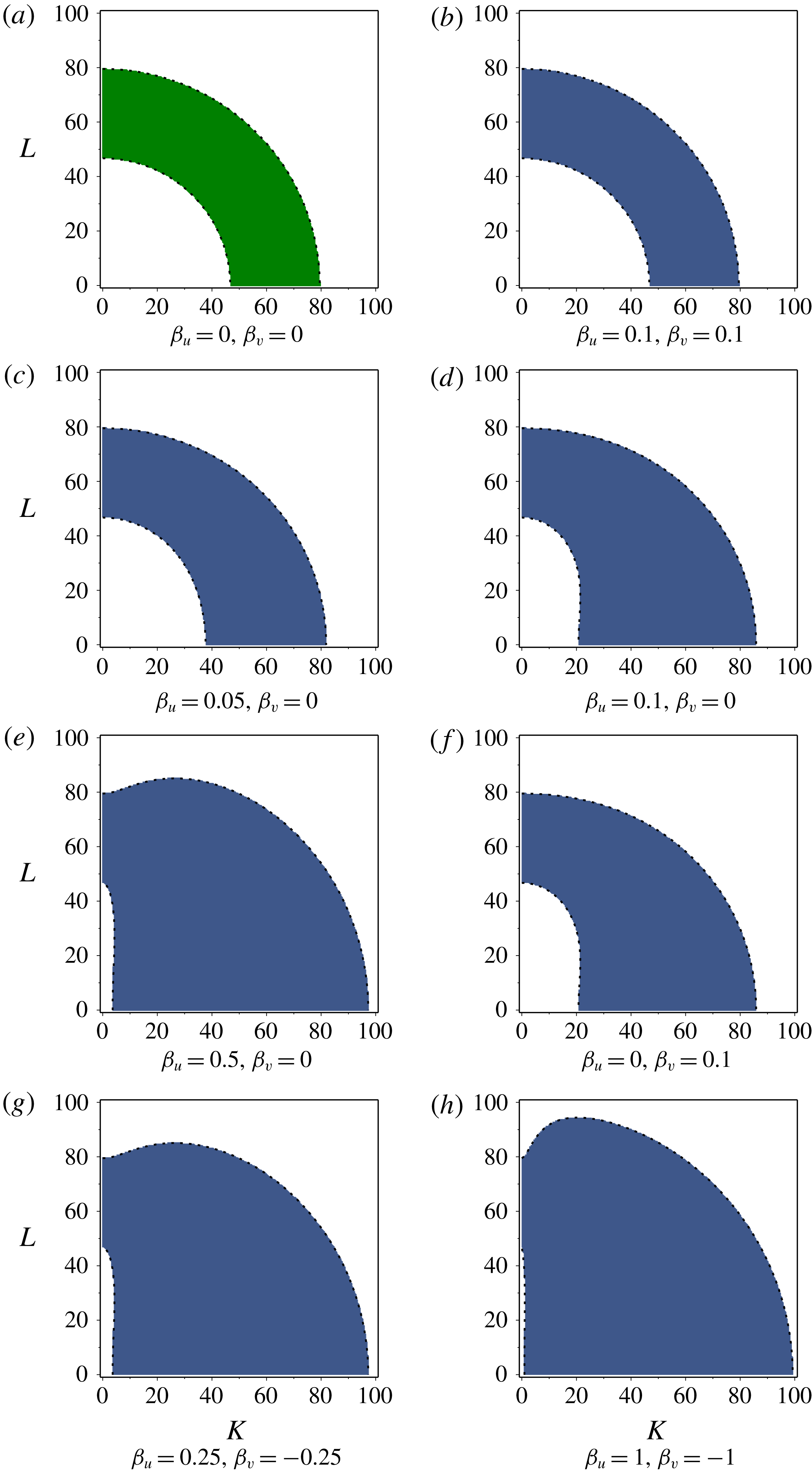
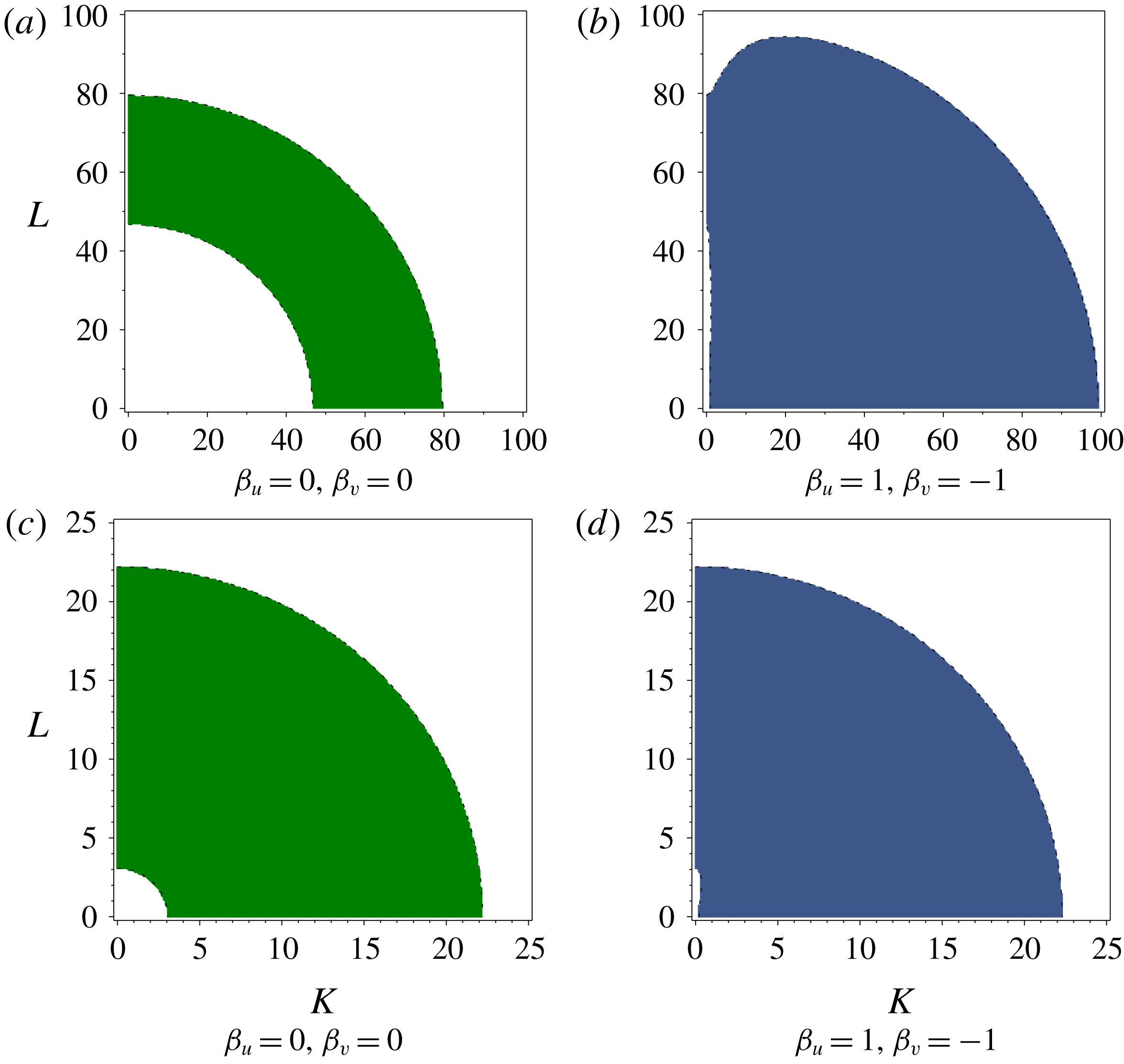
. We give examples of this in figures 1–2.
Instability regions of wavenumber space
 $(K,L)=(\unicode[STIX]{x1D6FC}k\unicode[STIX]{x03C0},|\boldsymbol{l}|)$
for Schnakenberg reaction kinetics given different values of the advection parameters
 $\unicode[STIX]{x1D6FD}_{u}$
and
 $\unicode[STIX]{x1D6FD}_{v}$
. We set
 $\unicode[STIX]{x1D6FF}_{u}=10^{-4}$
,
 $\unicode[STIX]{x1D6FF}_{v}=2\times 10^{-3}$
,
 $a=0.01$
and
 $b=1.65$
. We scale the spectrum like
 $K=\unicode[STIX]{x1D6FC}k\unicode[STIX]{x03C0}$
and
 $L=|\boldsymbol{l}|$
, hence the aspect ratio
 $\unicode[STIX]{x1D6FC}$
will only scale the instability region. White regions indicate
 $\text{Re}(\unicode[STIX]{x1D706}_{\pm ,k,\boldsymbol{l}})<0$
and hence stability. Green regions indicate
 $\text{Re}(\unicode[STIX]{x1D706}_{\pm ,k,\boldsymbol{l}})>0$
and
 $\text{Im}(\unicode[STIX]{x1D706}_{\pm ,k,\boldsymbol{l}})=0$
, corresponding to the Turing space
 ${\mathcal{T}}$
of (2.21), hence any patterns which develop would be stationary. Blue regions indicate
 $\text{Re}(\unicode[STIX]{x1D706}_{\pm ,k,\boldsymbol{l}})>0$
and
 $\text{Im}(\unicode[STIX]{x1D706}_{\pm ,k,\boldsymbol{l}})\neq 0$
, hence spatio-temporal patterns, including patterns which translate with the flow.

Instability regions of wavenumber space
 $(K,L)=(\unicode[STIX]{x1D6FC}k\unicode[STIX]{x03C0},|\boldsymbol{l}|)$
for Schnakenberg reaction kinetics given different parameter values. In (a,c) we take
 $\unicode[STIX]{x1D6FD}_{u}=\unicode[STIX]{x1D6FD}_{v}=0$
, while in (b,d) we take the maximal difference in advection parameters, hence
 $\unicode[STIX]{x1D6FD}_{u}=1$
,
 $\unicode[STIX]{x1D6FD}_{v}=-1$
. (Recall that the advection parameters scale like
 $-1\leqslant \unicode[STIX]{x1D6FD}_{u},\unicode[STIX]{x1D6FD}_{v}\leqslant 1$
, and it is the differential advection strength
 $|\unicode[STIX]{x1D6FD}_{u}-\unicode[STIX]{x1D6FD}_{v}|$
which shall matter for changing the instability region, hence the maximal differential advection is 2.) We set (a,b)
 $\unicode[STIX]{x1D6FF}_{u}=10^{-4}$
,
 $\unicode[STIX]{x1D6FF}_{v}=2\times 10^{-3}$
,
 $a=0.01$
and
 $b=1.65$
; (c,d)
 $\unicode[STIX]{x1D6FF}_{u}=1.6\times 10^{-3}$
,
 $\unicode[STIX]{x1D6FF}_{v}=1.6\times 10^{-1}$
,
 $a=0.1$
and
 $b=0.99$
. We scale the spectrum like
 $K=\unicode[STIX]{x1D6FC}k\unicode[STIX]{x03C0}$
and
 $L=|\boldsymbol{l}|$
, hence the aspect ratio
 $\unicode[STIX]{x1D6FC}$
will only scale the instability region. White regions indicate
 $\text{Re}(\unicode[STIX]{x1D706}_{\pm ,k,\boldsymbol{l}})<0$
and hence stability. Green regions indicate
 $\text{Re}(\unicode[STIX]{x1D706}_{\pm ,k,\boldsymbol{l}})>0$
and
 $\text{Im}(\unicode[STIX]{x1D706}_{\pm ,k,\boldsymbol{l}})=0$
, corresponding to the Turing space
 ${\mathcal{T}}$
of (2.21), hence any patterns which develop would be stationary. Blue regions indicate
 $\text{Re}(\unicode[STIX]{x1D706}_{\pm ,k,\boldsymbol{l}})>0$
and
 $\text{Im}(\unicode[STIX]{x1D706}_{\pm ,k,\boldsymbol{l}})\neq 0$
, hence spatio-temporal patterns, including patterns which translate with the flow.

In figure 1 we fix all system parameters save for advection, and then determine how the Turing space will change with a change in advection parameters. Panel (a) corresponds to zero advection, in which case we recover the region for the standard Turing instability for our choice of reaction kinetics and diffusion parameters, as derived in § 2.3. Increasing both advection parameters in the same manner, we see in panel (b) that the instability now corresponds to temporal eigenvalues with non-zero imaginary part. The size of the region is unchanged from panel (a), as both advection parameters are equal and hence there is no differential flow; as mentioned in previous sections, we need
 $\unicode[STIX]{x1D6FD}_{u}-\unicode[STIX]{x1D6FD}_{v}\neq 0$
in order to change the real part of the temporal eigenvalues away from what would be seen in a standard Turing instability. This is shown in subsequent panels, where we consider
 $\unicode[STIX]{x1D6FD}_{u}\neq \unicode[STIX]{x1D6FD}_{v}$
. In panels (c–e) we gradually increase the size of
 $\unicode[STIX]{x1D6FD}_{u}$
while fixing
 $\unicode[STIX]{x1D6FD}_{v}=0$
, finding that the extent of the Turing space increases as well. Note that this increase in the extent of the Turing space is the same whether we change
 $\unicode[STIX]{x1D6FD}_{u}$
and
 $\unicode[STIX]{x1D6FD}_{v}$
, as evidenced from comparing panels (c,f). Again, it is only the relative difference between these two parameters which will determine the change in the Turing space. In panels (g,h) we increase the difference in advection parameters further. Since we have scaled the problem so that
 $-1\leqslant \unicode[STIX]{x1D6FD}_{u},\unicode[STIX]{x1D6FD}_{v}\leqslant 1$
, panel (h) shows the maximum possible extent of the Turing space for these parameter values.
Figure 1 demonstrates that when advection acts differently on each type of morphogen, the result is to enlarge the Turing space, resulting in a wider variety of feasible unstable modes, and hence a greater variety of possible patterns. We further highlight this in figure 2, where we consider three different parameter sets and plot both standard Turing spaces (for
 $\unicode[STIX]{x1D6FD}_{u}=\unicode[STIX]{x1D6FD}_{v}=0$
) and enlarged Turing spaces due to maximal differential advection. Regardless of whether or not there is differential flow between the two morphogens, there will still be the possibility for spatio-temporal patterning, as even
 $\unicode[STIX]{x1D6FD}_{u}=\unicode[STIX]{x1D6FD}_{v}\neq 0$
will result in temporal eigenvalues with non-zero imaginary part. Therefore, the generic behaviour of patterns will be to move, rather than to remain stationary. As we shall later show through simulations, when advection varies in space, there will be an even greater possibility for patterns, with one type of pattern forming in a region of faster flow, and another pattern forming in a region of slower flow.
4 Pattern formation in channels, pipes and ducts
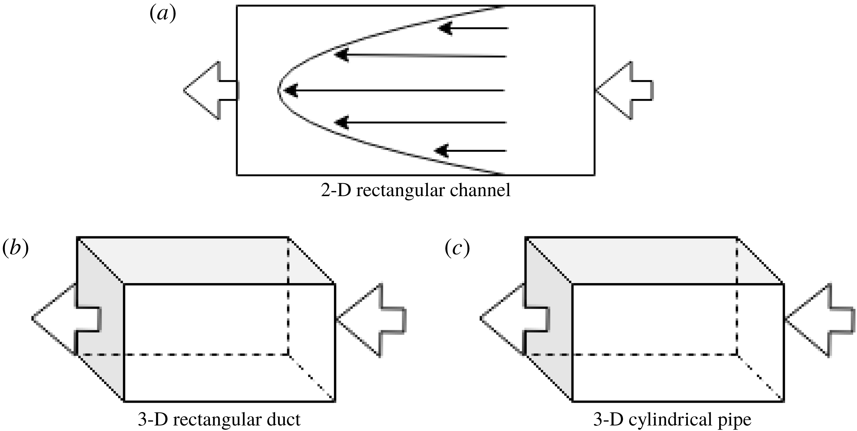
Having outlined the general approach for detecting instabilities in reaction–diffusion–advection systems in complex domains, we shall now present several analytical examples corresponding to common flow basins, such as a 2-D rectangular channel, 3-D cylindrical pipe and 3-D rectangular duct (see figure 3 for diagrams of each geometry). We use these geometries for numerical simulations, which will verify the onset of instabilities which we approximate analytically with the linear theory.
While the governing equations in each geometry are difficult to analyse in detail, for specific reaction kinetics they are amenable to numerical simulation using general-purpose software, without the need for specialized numerical methods (although such approaches can be useful in the context of reaction–diffusion–advection systems). Here we show simulations of the reaction–diffusion–advection equations in the three geometries described in the cases of Stokes flow and averaged advection. These were computed using the finite-element software COMSOL (see Dickinson, Ekström & Fontes Reference Dickinson, Ekström and Fontes2014, for a relevant review). In each case we discretized the spatial domain into triangular or tetrahedral elements, and interpolated the solution using second-order finite elements. The reaction–diffusion–advection system was evolved in time using a standard backward-difference-formula time stepping scheme with a tolerance of
 $10^{-5}$
, and an initial time step of
 $10^{-6}$
, though the solver adaptively changed the time step depending on the current problem structure. For the 2-D channel we used
 $24\,912$
triangular elements, for the 3-D pipe flow we used
 $39\,281$
tetrahedral elements and for the 3-D duct we used
 $32\,429$
tetrahedral elements.
We compared select (uniform flow) simulations to finite-difference simulations carried out in Matlab, and obtained solutions which agreed for sufficiently fine meshes. Additional spatial and temporal convergence checks were carried out to ensure the accuracy of our numerical method, though we remark that identical initial data had to be used in each case. For each geometry, a normally distributed random spatial noise with standard deviation
 $10^{-3}$
was added to the homogeneous initial data to observe patterning due to the diffusion–advection instabilities described in the preceding section. Specifically, we set
 $u(x,y,0)=u^{\ast }+\unicode[STIX]{x1D701}_{u}(x,y)$
and
 $v(x,y,0)=v^{\ast }+\unicode[STIX]{x1D701}_{v}(x,y)$
, where
 $\unicode[STIX]{x1D701}_{u},\unicode[STIX]{x1D701}_{v}\sim {\mathcal{N}}(0,10^{-3})$
are independently distributed for each morphogen and each spatial mesh point (and similarly in the 3-D case). We used the same seed to observe the same realization of the random perturbation in each case within the same geometry. For brevity we only show plots of the activator,
 $u$
, in all figures, but note that one may obtain similar patterning in the inhibitor.
A schematic diagram of the three periodic geometries considered in this section, a 2-D rectangular channel (a), a 3-D rectangular duct (b) and a 3-D cylindrical pipe (c). We use large arrows to represent periodic flow conditions on boundaries, and assume no flux of morphogens and no slip of fluid on all other boundaries. The parabolic profile of fluid velocity is sketched in the 2-D rectangular channel in (a).

4.1 Two-dimensional rectangular channel
4.1.1 Model for a 2-D rectangular channel
Consider a rectangular channel with dimensions
 $\tilde{x}\in [0,L]$
,
 ${\tilde{y}}\in [0,H]$
. We assume that the flow within the rectangular channel is steady, parallel and laminar. The pressure gradient is assumed constant, and is applied in the
 $\tilde{x}$
direction, so that
 $p=P(\tilde{x})$
. We ignore the effects of gravity. By imposing no-slip conditions at the walls, the boundary conditions are velocity equal to zero at
 ${\tilde{y}}=0$
and
 ${\tilde{y}}=H$
. We consider
 $\boldsymbol{A}=(A_{\tilde{x}},A_{{\tilde{y}}})$
, where
 $A_{\tilde{x}}$
and
 $A_{{\tilde{y}}}$
are velocities in the
 $\tilde{x}$
and
 ${\tilde{y}}$
directions, respectively. As we assume a flow driven by a constant pressure gradient, for ease of notation we denote
 $\text{d}P/\text{d}\tilde{x}=P_{\unicode[STIX]{x1D6E5}}$
. After standard calculations, we have
 $$\begin{eqnarray}\boldsymbol{A}=\left(\frac{P_{\unicode[STIX]{x1D6E5}}}{2\unicode[STIX]{x1D708}}{\tilde{y}}({\tilde{y}}-H),0\right),\end{eqnarray}$$
which is the Poiseuille flow for a 2-D rectangular channel. We choose the non-dimensional parameters as in § 2.1, and note that
 $A_{avg}=-1/6$
, hence
 $A(y)=6y(1-y)$
. The non-dimensional system modelling the reaction–diffusion–advection system in a 2-D rectangular channel then reads
 $$\begin{eqnarray}\displaystyle & \displaystyle \frac{\unicode[STIX]{x2202}u}{\unicode[STIX]{x2202}t}=f(u,v)+\unicode[STIX]{x1D6FF}_{u}\frac{\unicode[STIX]{x2202}^{2}u}{\unicode[STIX]{x2202}y^{2}}+\unicode[STIX]{x1D6FF}_{u}\unicode[STIX]{x1D6FC}^{2}\frac{\unicode[STIX]{x2202}^{2}u}{\unicode[STIX]{x2202}x^{2}}+6\unicode[STIX]{x1D6FD}_{u}y(1-y)\frac{\unicode[STIX]{x2202}u}{\unicode[STIX]{x2202}x}, & \displaystyle\end{eqnarray}$$
 $$\begin{eqnarray}\displaystyle & \displaystyle \frac{\unicode[STIX]{x2202}v}{\unicode[STIX]{x2202}t}=g(u,v)+\unicode[STIX]{x1D6FF}_{v}\frac{\unicode[STIX]{x2202}^{2}v}{\unicode[STIX]{x2202}y^{2}}+\unicode[STIX]{x1D6FF}_{v}\unicode[STIX]{x1D6FC}^{2}\frac{\unicode[STIX]{x2202}^{2}v}{\unicode[STIX]{x2202}x^{2}}+6\unicode[STIX]{x1D6FD}_{v}y(1-y)\frac{\unicode[STIX]{x2202}v}{\unicode[STIX]{x2202}x}, & \displaystyle\end{eqnarray}$$
 $$\begin{eqnarray}\displaystyle & \displaystyle u(0,y,t)=u(1,y,t),\quad v(0,y,t)=v(1,y,t), & \displaystyle\end{eqnarray}$$
 $$\begin{eqnarray}\displaystyle & \displaystyle \frac{\unicode[STIX]{x2202}u}{\unicode[STIX]{x2202}x}(0,y,t)=\frac{\unicode[STIX]{x2202}u}{\unicode[STIX]{x2202}x}(1,y,t),\quad \frac{\unicode[STIX]{x2202}v}{\unicode[STIX]{x2202}x}(0,y,t)=\frac{\unicode[STIX]{x2202}v}{\unicode[STIX]{x2202}x}(1,y,t), & \displaystyle\end{eqnarray}$$
 $$\begin{eqnarray}\displaystyle & \displaystyle \frac{\unicode[STIX]{x2202}u}{\unicode[STIX]{x2202}y}(x,0,t)=\frac{\unicode[STIX]{x2202}v}{\unicode[STIX]{x2202}y}(x,0,t)=\frac{\unicode[STIX]{x2202}u}{\unicode[STIX]{x2202}y}(x,1,t)=\frac{\unicode[STIX]{x2202}v}{\unicode[STIX]{x2202}y}(x,1,t)=0. & \displaystyle\end{eqnarray}$$
Since we are interested in loss of stability of spatially uniform states for the chemical species, we shall choose initial conditions of the form
 $$\begin{eqnarray}u(x,y,0)=u^{\ast }+U(x,y),\quad v(x,y,0)=v^{\ast }+V(x,y),\end{eqnarray}$$
where
 $u^{\ast },v^{\ast }$
are the spatially uniform steady states satisfying the algebraic equations
 $f(u^{\ast },v^{\ast })=g(u^{\ast },v^{\ast })=0$
while we take small perturbations with amplitudes
 $|U(x,y)|\ll 1$
,
 $|V(x,y)|\ll 1$
.
4.1.2 Instability in a 2-D rectangular channel flow
We first consider a flow within a 2-D rectangular channel, as described in § 4.1. Linearization of the equations (4.2a )–(4.2b ) gives
 $$\begin{eqnarray}\displaystyle & \displaystyle \frac{\unicode[STIX]{x2202}\hat{u} }{\unicode[STIX]{x2202}t}=f_{u}^{\ast }\hat{u} +f_{v}^{\ast }\hat{v}+\unicode[STIX]{x1D6FF}_{u}\frac{\unicode[STIX]{x2202}^{2}\hat{u} }{\unicode[STIX]{x2202}y^{2}}+\unicode[STIX]{x1D6FF}_{u}\unicode[STIX]{x1D6FC}^{2}\frac{\unicode[STIX]{x2202}^{2}\hat{u} }{\unicode[STIX]{x2202}x^{2}}+6\unicode[STIX]{x1D6FD}_{u}y(1-y)\frac{\unicode[STIX]{x2202}\hat{u} }{\unicode[STIX]{x2202}x}, & \displaystyle\end{eqnarray}$$
 $$\begin{eqnarray}\displaystyle & \displaystyle \frac{\unicode[STIX]{x2202}\hat{v}}{\unicode[STIX]{x2202}t}=g_{u}^{\ast }\hat{u} +g_{v}^{\ast }\hat{v}+\unicode[STIX]{x1D6FF}_{v}\frac{\unicode[STIX]{x2202}^{2}\hat{v}}{\unicode[STIX]{x2202}y^{2}}+\unicode[STIX]{x1D6FF}_{v}\unicode[STIX]{x1D6FC}^{2}\frac{\unicode[STIX]{x2202}^{2}\hat{v}}{\unicode[STIX]{x2202}x^{2}}+6\unicode[STIX]{x1D6FD}_{v}y(1-y)\frac{\unicode[STIX]{x2202}\hat{v}}{\unicode[STIX]{x2202}x}. & \displaystyle\end{eqnarray}$$
Let
 $$\begin{eqnarray}\left(\begin{array}{@{}c@{}}\hat{u} \\ \hat{v}\end{array}\right)=\left(\begin{array}{@{}c@{}}\overline{u}\\ \overline{v}\end{array}\right)\exp (\text{i}k\unicode[STIX]{x03C0}x+\unicode[STIX]{x1D706}t)w(y),\end{eqnarray}$$
where
 $\overline{u}$
and
 $\overline{v}$
are constants. Then, we obtain the spectral problem
 $$\begin{eqnarray}\displaystyle \unicode[STIX]{x1D706}\left(\begin{array}{@{}cc@{}}1 & 0\\ 0 & 1\end{array}\right)\left(\begin{array}{@{}c@{}}\overline{u}\\ \overline{v}\end{array}\right)w(y) & = & \displaystyle \left\{\left[\left(\begin{array}{@{}cc@{}}f_{u}^{\ast } & f_{v}^{\ast }\\ g_{u}^{\ast } & g_{v}^{\ast }\end{array}\right)-\unicode[STIX]{x1D6FC}^{2}k^{2}\unicode[STIX]{x03C0}^{2}\left(\begin{array}{@{}cc@{}}\unicode[STIX]{x1D6FF}_{u} & 0\\ 0 & \unicode[STIX]{x1D6FF}_{v}\end{array}\right)\right]w(y)+\left(\begin{array}{@{}cc@{}}\unicode[STIX]{x1D6FF}_{u} & 0\\ 0 & \unicode[STIX]{x1D6FF}_{v}\end{array}\right)w^{\prime \prime }(y)\right.\nonumber\\ \displaystyle & & \displaystyle +\left.6\text{i}\unicode[STIX]{x03C0}k\left(\begin{array}{@{}cc@{}}\unicode[STIX]{x1D6FD}_{u} & 0\\ 0 & \unicode[STIX]{x1D6FD}_{v}\end{array}\right)y(1-y)w(y)\right\}\left(\begin{array}{@{}c@{}}\overline{u}\\ \overline{v}\end{array}\right).\end{eqnarray}$$
The spatial eigenvalue problem for
 $w(y)$
takes the form
 $$\begin{eqnarray}\left(\begin{array}{@{}cc@{}}\unicode[STIX]{x1D6FF}_{u} & 0\\ 0 & \unicode[STIX]{x1D6FF}_{v}\end{array}\right)w^{\prime \prime }(y)+6\text{i}\unicode[STIX]{x03C0}k\left(\begin{array}{@{}cc@{}}\unicode[STIX]{x1D6FD}_{u} & 0\\ 0 & \unicode[STIX]{x1D6FD}_{v}\end{array}\right)y(1-y)w(y)=\left(\begin{array}{@{}cc@{}}\unicode[STIX]{x1D71E}_{1} & 0\\ 0 & \unicode[STIX]{x1D71E}_{2}\end{array}\right)w(y).\end{eqnarray}$$
The eigenvalue problem (4.7) is consistent provided that
 $\unicode[STIX]{x1D6FD}_{u}/\unicode[STIX]{x1D6FF}_{u}=\unicode[STIX]{x1D6FD}_{v}/\unicode[STIX]{x1D6FF}_{v}$
,
 $\unicode[STIX]{x1D71E}_{1}=\unicode[STIX]{x1D6FF}_{u}\unicode[STIX]{x1D707}$
,
 $\unicode[STIX]{x1D71E}_{2}=\unicode[STIX]{x1D6FF}_{v}\unicode[STIX]{x1D707}$
, where
 $\unicode[STIX]{x1D707}$
is an eigenvalue of the scalar eigenvalue problem
 $$\begin{eqnarray}w^{\prime \prime }(y)+6\text{i}\unicode[STIX]{x03C0}k\frac{\unicode[STIX]{x1D6FD}_{u}}{\unicode[STIX]{x1D6FF}_{u}}y(1-y)w(y)=\unicode[STIX]{x1D707}w(y).\end{eqnarray}$$
The eigenfunction solutions to (4.8) are products of hypergeometric functions and exponential terms, and it is prohibitively complicated to obtain a reasonable analytic approximation to the eigenvalues
 $\unicode[STIX]{x1D707}$
, so we omit these details. However, as discussed earlier, we do know certain properties of the eigenvalues. Let us denote
 $\unicode[STIX]{x1D707}=\unicode[STIX]{x1D707}_{\ell ,k}(\unicode[STIX]{x1D6FD}_{u}/\unicode[STIX]{x1D6FF}_{u})=\hat{\unicode[STIX]{x1D707}}_{\ell }((\unicode[STIX]{x1D6FD}_{u}/\unicode[STIX]{x1D6FF}_{u})k)$
, for
 $\ell =0,1,2,\ldots$
. Then,
 $\text{Re}(\hat{\unicode[STIX]{x1D707}}_{\ell }(a))\leqslant 0$
, while
 $\text{Im}(\hat{\unicode[STIX]{x1D707}}_{\ell }(a))\neq 0$
for
 $a\neq 0$
in general.
Writing
 $\unicode[STIX]{x1D707}_{\ell ,k}=\text{Re}(\unicode[STIX]{x1D707}_{\ell ,k}(\unicode[STIX]{x1D6FD}_{u}/\unicode[STIX]{x1D6FF}_{u}))+\text{i}\text{Im}(\unicode[STIX]{x1D707}_{\ell ,k}(\unicode[STIX]{x1D6FD}_{u}/\unicode[STIX]{x1D6FF}_{u}))$
, the spectral problem (4.6) now is put into the form
 $$\begin{eqnarray}\displaystyle \unicode[STIX]{x1D706}\left(\begin{array}{@{}cc@{}}1 & 0\\ 0 & 1\end{array}\right)\left(\begin{array}{@{}c@{}}\overline{u}\\ \overline{v}\end{array}\right) & = & \displaystyle \left\{\left(\begin{array}{@{}cc@{}}f_{u}^{\ast } & f_{v}^{\ast }\\ g_{u}^{\ast } & g_{v}^{\ast }\end{array}\right)-(\unicode[STIX]{x1D6FC}^{2}k^{2}\unicode[STIX]{x03C0}^{2}+|\text{Re}(\unicode[STIX]{x1D707}_{\ell ,k}(\unicode[STIX]{x1D6FD}_{u}/\unicode[STIX]{x1D6FF}_{u}))|)\left(\begin{array}{@{}cc@{}}\unicode[STIX]{x1D6FF}_{u} & 0\\ 0 & \unicode[STIX]{x1D6FF}_{v}\end{array}\right)\right.\nonumber\\ \displaystyle & & \displaystyle +\left.\text{i}\text{Im}(\unicode[STIX]{x1D707}_{\ell ,k}(\unicode[STIX]{x1D6FD}_{u}/\unicode[STIX]{x1D6FF}_{u}))\left(\begin{array}{@{}cc@{}}\unicode[STIX]{x1D6FF}_{u} & 0\\ 0 & \unicode[STIX]{x1D6FF}_{v}\end{array}\right)\right\}\left(\begin{array}{@{}c@{}}\overline{u}\\ \overline{v}\end{array}\right).\end{eqnarray}$$
We define
 $$\begin{eqnarray}\displaystyle & \displaystyle {\mathcal{P}}(\ell ,k)=\left(\begin{array}{@{}cc@{}}f_{u}^{\ast } & f_{v}^{\ast }\\ g_{u}^{\ast } & g_{v}^{\ast }\end{array}\right)-(\unicode[STIX]{x1D6FC}^{2}k^{2}\unicode[STIX]{x03C0}^{2}+|\text{Re}(\unicode[STIX]{x1D707}_{\ell ,k}(\unicode[STIX]{x1D6FD}_{u}/\unicode[STIX]{x1D6FF}_{u}))|)\left(\begin{array}{@{}cc@{}}\unicode[STIX]{x1D6FF}_{u} & 0\\ 0 & \unicode[STIX]{x1D6FF}_{v}\end{array}\right), & \displaystyle\end{eqnarray}$$
 $$\begin{eqnarray}\displaystyle & \displaystyle {\mathcal{Q}}(\ell ,k)=\text{Im}(\unicode[STIX]{x1D707}_{\ell ,k}(\unicode[STIX]{x1D6FD}_{u}/\unicode[STIX]{x1D6FF}_{u}))\left(\begin{array}{@{}cc@{}}\unicode[STIX]{x1D6FF}_{u} & 0\\ 0 & \unicode[STIX]{x1D6FF}_{v}\end{array}\right). & \displaystyle\end{eqnarray}$$
Then, applying (3.16)–(3.17), we see that the imaginary part of the temporal eigenvalues
 $\unicode[STIX]{x1D706}_{\pm ,\ell ,k}$
is generically non-zero, hence we expect spatio-temporal patterning whenever
 $\text{Re}(\unicode[STIX]{x1D706}_{\pm ,\ell ,k})>0$
for at least one pair of
 $\ell$
and
 $k$
, according to (3.16).
Due to spatial heterogeneity, explicit closed form calculation of eigenvalues is not possible for the heterogeneous problem, yet the above analysis does indicate that the onset of instabilities should be fairly generic within the proper parameter regime. In order to press further with our analysis, we now turn our attention to averaged flow in a 2-D rectangular channel. This will simplify the spatial eigenvalue problem, and hence some information on the precise structure of the emergent patterning will be lost. However, this approach is still useful in understanding the onset of the instability, as it will not require the restriction between the advection and diffusion parameters which were required for the spatially heterogeneous problem to be self-adjoint.
Taking the average of the advection over a cross-section, the dimensionless reaction–advection–diffusion equations (4.2a )–(4.2b ) become
 $$\begin{eqnarray}\displaystyle & \displaystyle \frac{\unicode[STIX]{x2202}u}{\unicode[STIX]{x2202}t}=f(u,v)+\unicode[STIX]{x1D6FF}_{u}\frac{\unicode[STIX]{x2202}^{2}u}{\unicode[STIX]{x2202}y^{2}}+\unicode[STIX]{x1D6FF}_{u}\unicode[STIX]{x1D6FC}^{2}\frac{\unicode[STIX]{x2202}^{2}u}{\unicode[STIX]{x2202}x^{2}}+\unicode[STIX]{x1D6FD}_{u}\frac{\unicode[STIX]{x2202}u}{\unicode[STIX]{x2202}x}, & \displaystyle\end{eqnarray}$$
 $$\begin{eqnarray}\displaystyle & \displaystyle \frac{\unicode[STIX]{x2202}v}{\unicode[STIX]{x2202}t}=g(u,v)+\unicode[STIX]{x1D6FF}_{v}\frac{\unicode[STIX]{x2202}^{2}v}{\unicode[STIX]{x2202}y^{2}}+\unicode[STIX]{x1D6FF}_{v}\unicode[STIX]{x1D6FC}^{2}\frac{\unicode[STIX]{x2202}^{2}v}{\unicode[STIX]{x2202}x^{2}}+\unicode[STIX]{x1D6FD}_{v}\frac{\unicode[STIX]{x2202}v}{\unicode[STIX]{x2202}x}, & \displaystyle\end{eqnarray}$$
while the boundary and initial conditions remain of the form (4.2c )–(4.2f ). Linearization of these equations gives
 $$\begin{eqnarray}\displaystyle & \displaystyle \frac{\unicode[STIX]{x2202}\hat{u} }{\unicode[STIX]{x2202}t}=f_{u}^{\ast }\hat{u} +f_{v}^{\ast }\hat{v}+\unicode[STIX]{x1D6FF}_{u}\frac{\unicode[STIX]{x2202}^{2}\hat{u} }{\unicode[STIX]{x2202}y^{2}}+\unicode[STIX]{x1D6FF}_{u}\unicode[STIX]{x1D6FC}^{2}\frac{\unicode[STIX]{x2202}^{2}\hat{u} }{\unicode[STIX]{x2202}x^{2}}+\unicode[STIX]{x1D6FD}_{u}\frac{\unicode[STIX]{x2202}\hat{u} }{\unicode[STIX]{x2202}x}, & \displaystyle\end{eqnarray}$$
 $$\begin{eqnarray}\displaystyle & \displaystyle \frac{\unicode[STIX]{x2202}\hat{v}}{\unicode[STIX]{x2202}t}=g_{u}^{\ast }\hat{u} +g_{v}^{\ast }\hat{v}+\unicode[STIX]{x1D6FF}_{v}\frac{\unicode[STIX]{x2202}^{2}\hat{v}}{\unicode[STIX]{x2202}y^{2}}+\unicode[STIX]{x1D6FF}_{v}\unicode[STIX]{x1D6FC}^{2}\frac{\unicode[STIX]{x2202}^{2}\hat{v}}{\unicode[STIX]{x2202}x^{2}}+\unicode[STIX]{x1D6FD}_{v}\frac{\unicode[STIX]{x2202}\hat{v}}{\unicode[STIX]{x2202}x}. & \displaystyle\end{eqnarray}$$
Let
 $$\begin{eqnarray}\left(\begin{array}{@{}c@{}}\hat{u} \\ \hat{v}\end{array}\right)=\left(\begin{array}{@{}c@{}}\overline{u}\\ \overline{v}\end{array}\right)\exp (\text{i}(k\unicode[STIX]{x03C0}x+l\unicode[STIX]{x03C0}y)+\unicode[STIX]{x1D706}t),\end{eqnarray}$$
where
 $\overline{u}$
and
 $\overline{v}$
are constants. Then,
 $$\begin{eqnarray}\unicode[STIX]{x1D706}\left(\begin{array}{@{}cc@{}}1 & 0\\ 0 & 1\end{array}\right)\left(\begin{array}{@{}c@{}}\overline{u}\\ \overline{v}\end{array}\right)=J\left(\begin{array}{@{}c@{}}\overline{u}\\ \overline{v}\end{array}\right),\end{eqnarray}$$
where
 $$\begin{eqnarray}J=\left(\begin{array}{@{}cc@{}}f_{u}^{\ast } & f_{v}^{\ast }\\ g_{u}^{\ast } & g_{v}^{\ast }\end{array}\right)-(l^{2}+\unicode[STIX]{x1D6FC}^{2}k^{2})\unicode[STIX]{x03C0}^{2}\left(\begin{array}{@{}cc@{}}\unicode[STIX]{x1D6FF}_{u} & 0\\ 0 & \unicode[STIX]{x1D6FF}_{v}\end{array}\right)+\unicode[STIX]{x03C0}\text{i}k\left(\begin{array}{@{}cc@{}}\unicode[STIX]{x1D6FD}_{u} & 0\\ 0 & \unicode[STIX]{x1D6FD}_{v}\end{array}\right).\end{eqnarray}$$
Following the approach of appendix A, we define
 $$\begin{eqnarray}\tilde{J}(l,k)=\left(\begin{array}{@{}cc@{}}f_{u}^{\ast } & f_{v}^{\ast }\\ g_{u}^{\ast } & g_{v}^{\ast }\end{array}\right)-\unicode[STIX]{x03C0}^{2}(l^{2}+\unicode[STIX]{x1D6FC}^{2}k^{2})\left(\begin{array}{@{}cc@{}}\unicode[STIX]{x1D6FF}_{u} & 0\\ 0 & \unicode[STIX]{x1D6FF}_{v}\end{array}\right),\end{eqnarray}$$
with
 $\text{tr}(\tilde{J}(l,k))<0$
(from stable reaction kinetics),
 $$\begin{eqnarray}\displaystyle & \displaystyle \unicode[STIX]{x1D6F7}(l,k)=(\text{tr}(\tilde{J}(l,k)))^{2}-4\det (\tilde{J}(l,k)), & \displaystyle\end{eqnarray}$$
 $$\begin{eqnarray}\displaystyle & \displaystyle \unicode[STIX]{x1D6F9}(l,k)=(g_{v}^{\ast }-f_{u}^{\ast }+(\unicode[STIX]{x1D6FF}_{u}-\unicode[STIX]{x1D6FF}_{v})(l^{2}+\unicode[STIX]{x1D6FC}^{2}k^{2})\unicode[STIX]{x03C0}^{2})^{2}, & \displaystyle\end{eqnarray}$$
 $$\begin{eqnarray}\displaystyle & \displaystyle \unicode[STIX]{x1D6E9}=\unicode[STIX]{x03C0}^{2}(\unicode[STIX]{x1D6FD}_{u}-\unicode[STIX]{x1D6FD}_{v})^{2}. & \displaystyle\end{eqnarray}$$
We then obtain
 $$\begin{eqnarray}\text{Re}(\unicode[STIX]{x1D706}_{\pm })=\frac{\text{tr}(\tilde{J})}{2}\pm \frac{1}{2^{3/2}}[\{\unicode[STIX]{x1D6F7}^{2}+2k^{2}\unicode[STIX]{x1D6E9}(\unicode[STIX]{x1D6F9}-2\unicode[STIX]{x1D6F7})+k^{4}{\unicode[STIX]{x1D6E9}^{2}\}}^{1/2}+\unicode[STIX]{x1D6F7}-k^{2}\unicode[STIX]{x1D6E9}]^{1/2}.\end{eqnarray}$$
With this, the system (4.12)–(4.13) exhibits a diffusion-driven instability provided: (i)
 $\operatorname{tr}(\tilde{J}(0,0))<0$
, (ii)
 $\det (\tilde{J}(0,0))>0$
and (iii) there exist
 $l,k\in \mathbb{Z}$
such that
 $\text{Re}(\unicode[STIX]{x1D706}_{+})$
in (4.23) is positive. Note that the dependence of the real part of the eigenvalues on the difference in the constant advections is consistent with earlier findings by Perumpanani et al. (Reference Perumpanani, Sherratt and Maini1995) and others.
Unlike in the classical Turing instability, however, we have that the imaginary part of
 $\unicode[STIX]{x1D706}_{\pm }$
is non-zero, even if the difference of the advection parameters is zero. Hence, we have an oscillatory Turing or Turing wave type instability (Yang et al.
Reference Yang, Dolnik, Zhabotinsky and Epstein2002; Yang & Epstein Reference Yang and Epstein2003) for non-zero advection, even if there is no change to the real part of the eigenvalues as is true when advection acting on
 $u$
and
 $v$
is the same. We expect that this will manifest patterns which move in time, or even less regular wave patterns. Temporal eigenvalues with non-zero imaginary part and resulting wave instabilities have previously been observed in reaction–diffusion–advection systems (Rovinsky & Menzinger Reference Rovinsky and Menzinger1992; Flach et al.
Reference Flach, Schnell and Norbury2007; Berenstein Reference Berenstein2012a
,Reference Berenstein
b
; Ghosh et al.
Reference Ghosh, Paul and Ray2016). This will typically correspond to translation of spatial patterns with the fluid flow.
In the case where the advection parameters are equal, we have
 $\unicode[STIX]{x1D6E9}=0$
, and the formula (4.23) reduces to
 $$\begin{eqnarray}\displaystyle \text{Re}(\unicode[STIX]{x1D706}_{\pm }) & = & \displaystyle \frac{\text{tr}(\tilde{J})}{2}\pm \frac{1}{2}\sqrt{\unicode[STIX]{x1D6F7}(l,k)}\nonumber\\ \displaystyle & = & \displaystyle \frac{\text{tr}(\tilde{J})}{2}\pm \frac{1}{2}\sqrt{(\text{tr}(\tilde{J}(l,k)))^{2}-4\det (\tilde{J}(l,k))}.\end{eqnarray}$$
Positivity of this expression in the presence of stable reaction kinetics is exactly the standard condition for Turing instability. However, note that the imaginary part
 $\text{Im}(\unicode[STIX]{x1D706}_{\pm })$
is non-zero unless both
 $\unicode[STIX]{x1D6FD}_{u}=\unicode[STIX]{x1D6FD}_{v}=0$
, i.e. when there is zero advection.
4.1.3 Pattern formation in the 2-D rectangular channel flow
We simulated (4.2), with the reaction kinetics given by (2.12), in order to explore the behaviour of patterned solutions under the different flow regimes discussed previously. In all cases we carried out simulations for a long time period (until
 $t=4\times 10^{4}$
), and record approximate times when the solutions have settled into either a steady state, or a translationally periodic steady state (e.g. when a fixed pattern is moving due to the advection in the flow, but is equivalent to a translated pattern). In some cases more complex behaviours than steady states or moving steady states occur, but we are observing either long-time asymptotic behaviour (or very long metastable states).
Spatial snapshots of solution
 $u$
to (4.2) using (2.12) at different times, and using different values of equal advection parameters
 $\unicode[STIX]{x1D6FD}_{u}=\unicode[STIX]{x1D6FD}_{v}=\unicode[STIX]{x1D6FD}$
. We set
 $\unicode[STIX]{x1D6FF}_{u}=10^{-4}$
,
 $\unicode[STIX]{x1D6FF}_{v}=10^{-2}$
,
 $\unicode[STIX]{x1D6FC}=1$
,
 $a=0.1$
and
 $b=0.99$
, and varied the advection parameters along each row as
 $\unicode[STIX]{x1D6FD}=0$
in (a–c),
 $\unicode[STIX]{x1D6FD}=0.1$
in (d–f),
 $\unicode[STIX]{x1D6FD}=0.3$
in (g–i) and
 $\unicode[STIX]{x1D6FD}=0.5$
in (j–l). Note that the flow in each panel (d–l) is from right to left.

We first demonstrate the influence of varying the advection parameters for a parameter regime which forms spot solutions without advection. For very small values of the advection (
 $\unicode[STIX]{x1D6FD}_{u}=\unicode[STIX]{x1D6FD}_{v}<0.01$
, not shown), spots form and move along the direction of the advection, although not uniformly due to the parabolic velocity profile of the flow. We show larger values of the advection in figure 4 where, in addition to moving along with the flow (movement toward the left), the spots display shearing behaviour and can locally form into steady stripe patterns aligned with the flow, for sufficiently large advection parameters. In each case, two or three qualitatively distinct regions are apparent. We note the spots on the horizontal boundaries move more slowly than their interior neighbours, but are dragged along due to both the flow and the nonlinear interactions. Spots on the very interior experience the highest levels of advection due to the flow, but it is also relatively uniform and so these spots only begin to deform at very high values of these parameters. Between these two regions we observe the most interesting behaviour, including spot shearing, due to the non-uniform flow between the centre and the horizontal boundaries. We also note that the transient behaviours clearly demonstrate the emergence of combinations of modes aligned with the flow in the horizontal direction. Finally, we mention that without advection the solution takes longer to stabilize to a stationary pattern than the case with advection takes to reach a translationally periodic steady state.
As figure 4 suggests that there are essentially three regions, it is worth taking inventory of how this relates to the patterns predicted by our instability analysis. The central region consists of spots which are formed through the Turing mechanism, and then advected with the flow. Provided these spots are both small enough and located at the centre of the domain, they will persist even for strong flows (
 $\unicode[STIX]{x1D6FD}_{u,v}=O(1)$
), since the wavelength of the unstable perturbation leading to the spots is sufficiently small relative to spatial variations in the velocity field. As such, the structure of the patterns in the centre of figure 4(i) are akin to the spots which develop in stationary flow case of figure 4(c), with the only difference being the motion of the pattern. This is well predicted by the linear instability analysis when the flow was approximated by a uniform flow, as in the case of spatially averaged advection described in the second half of § 4.1.2. Likewise, if the spot patterns are small enough, then a row of spots may pin to the boundaries of the domain in the direction orthogonal to the flow. For small
 $\unicode[STIX]{x1D6FD}_{u,v}$
these patterns will be similar in size and shape to those formed in the static case (compare the spots appearing on the boundaries of figure 4
c,f), in which case the spatially averaged analysis still provides a reasonable prediction of the pattern which develops. As such, the analysis carried out by approximating the flow as uniform in space (see appendix A) is a reasonable approximation in both regimes, without the need for more advanced spectral theory.
Between these two regions, there is a third regime consisting of sheared patterns, eventually giving way to stripes or bands for strong enough flow. This is not predicted well by the spatially averaged theory, as within this region there is a strong velocity gradient in the direction orthogonal to the flow. While in other regions, standard Turing patterns form and are then advected while maintaining their overall form, it is in this region where the simulations differ most from the standard Turing patterns (as seen when comparing figure 4
c with i,l). For cases such as this, one must consider the more general spectral analysis outlined in § 3.2. We consider a velocity field with constant gradient in space, e.g.
 $A(y)=y$
, in order to better understand this shear region. This is a reasonable approximation provided that the patterns formed are small relative to the global velocity field for the flow, in which case curvature resulting in a parabolic flow can be locally approximated by a constant gradient flow (with a Couette flow type profile) within the shear zone; such is the case in figure 4. Details of the resulting spectral problem are given in appendix B. To summarize, while the spectrum and hence Turing space are similar to that of the uniform flow, the eigenfunctions take the form
 $\text{e}^{\text{i}kx}w_{\ell }(y)$
, with
 $w_{\ell }(y)$
asymmetric over
 $y\in [0,1]$
, with the degree of asymmetry increasing as the strength of the flow is increased. This is in contrast to the symmetric eigenfunctions
 $\text{e}^{\text{i}kx}\text{e}^{\text{i}\ell y}$
obtained in the case of uniform flow. We hypothesize that the asymmetry of higher modes prevents their selection under the full nonlinear dynamics, resulting in the lowest (constant) mode being selected, resulting in a band which is constant in
 $y$
and varies in
 $x$
over the same length scale which defines a spot. This is exactly what is observed in figure 4(i,l). We shall later demonstrate similar behaviour in shear zones emergent in 3-D simulations.
We next consider parameters where labyrinthine solutions form without advection in figure 5. Due to the periodic boundary condition in the
 $x$
direction, even on the static domain we observe a tendency for these solutions to align with this axis (and this is consistent across many different random initial data). If the advection was sufficiently large (approximately greater than or equal to
 $0.001$
), then these solutions were driven into a perfectly aligned stripe solution which then did not vary in time. For advection smaller than this, we observed movement of the overall pattern as before, which becomes noticeable due to the breaking of the stripe patterns near the boundaries. For some values of the advection, these patterns entered a time-dependent behaviour where, in addition to translating along the flow, stripes near the boundary would periodically break apart and reform. While this effect was small, it motivated us to consider different kinds of stripe patterns to try and isolate a mechanism underlying this phenomenon, which we now describe.
In figures 6–7 we plot solutions for different parameters which admit striped patterns. We see that without advection, stripes form and align along the
 $y$
axis. When advection is turned on, these stripes move but also bend to accommodate the profile of the flow. Due to the lack of flow at the boundaries, this requires dragging the part of the stripe at the boundary much more slowly than the centre. For these parameters, we see that this can lead to an oscillating break-up of the parts of the stripe at the boundaries with the rest, as shown in figure 7. This occurs first for one side and then the other, with a relatively quick separation leading to the larger stripe attaching to the spot further downstream. The movement of stripes occurs on the scale of
 $O(10^{2})$
time units, the separation and reconnection on the scale of
 $O(10^{1})$
time units and the time between these events on the scale of
 $O(10^{3})$
time units, leading us to suspect that some kind of tension builds up in the stripe which is released at each of these periodic events. An initial asymmetry in the stripe formation leads these to occur separately at each boundary.
Spatial snapshots of solution
 $u$
to (4.2) using (2.12) at different times, and using different values of equal advection parameters
 $\unicode[STIX]{x1D6FD}_{u}=\unicode[STIX]{x1D6FD}_{v}=\unicode[STIX]{x1D6FD}$
. We set
 $\unicode[STIX]{x1D6FF}_{u}=10^{-4}$
,
 $\unicode[STIX]{x1D6FF}_{v}=2\times 10^{-3}$
,
 $\unicode[STIX]{x1D6FC}=1$
,
 $a=0.01$
and
 $b=1.65$
, and varied the advection parameters along each row as
 $\unicode[STIX]{x1D6FD}=0$
in (a–c),
 $\unicode[STIX]{x1D6FD}=10^{-5}$
in (d–f),
 $\unicode[STIX]{x1D6FD}=0.001$
in (g–i),
 $\unicode[STIX]{x1D6FD}=0.01$
in (j–l) and
 $\unicode[STIX]{x1D6FD}=0.1$
in (m–o). Note that the flow in each panel is from right to left. Note that the flow in each panel (d–o) is from right to left.

Spatial snapshots of solution
 $u$
to (4.2) using (2.12) at different times, and using different values of equal advection parameters
 $\unicode[STIX]{x1D6FD}_{u}=\unicode[STIX]{x1D6FD}_{v}=\unicode[STIX]{x1D6FD}$
. We set
 $\unicode[STIX]{x1D6FF}_{u}=4\times 10^{-4}$
,
 $\unicode[STIX]{x1D6FF}_{v}=8\times 10^{-3}$
,
 $\unicode[STIX]{x1D6FC}=1$
,
 $a=0.05$
and
 $b=1.65$
, and varied the advection parameters along each row as
 $\unicode[STIX]{x1D6FD}=0$
in (a–c), and
 $\unicode[STIX]{x1D6FD}=2\times 10^{-4}$
in (d–f). Note that the flow in each panel (d–f) is from right to left.

Further simulations of the solution
 $u$
from figure 6(d–f). Note that the flow in all panels is from right to left.

We now discuss simulations using uniform flow-driven advection. Constant uniform advection for small advection parameters (either being of order
 $0.01$
or less) leads to similar patterns as the stationary cases without advection. Namely, we observe spot movement, and stripe formation, but these all occur uniformly in
 $y$
, and depend almost entirely on the kinetic and diffusive parameters used, rather than any effect due to the advection. As an example, in figure 8(a–c), we show simulations where a labyrinthine pattern forms and is carried along uniformly in the flow. Here, the final snapshot is qualitatively similar to the stationary solution in figure 5(c), but we note that this pattern is moving rapidly to the left, such that it is periodic with a period of approximately
 $10$
units of time. In this slow flow regime, these results are consistent, up to a sign, with a change of coordinates to a moving frame
 $\tilde{x}=x-\unicode[STIX]{x1D6FD}_{u}t$
. In this case,
 $\unicode[STIX]{x1D6FD}_{u}=\unicode[STIX]{x1D6FD}_{v}$
, but qualitatively we observe the same dynamical behaviour, with possibly different speeds, if these advection parameters are unequal. We now describe this in some detail, for both uniform and Poiseuille flow.
Spatial snapshots of solution
 $u$
to (4.12)–(4.13) using (2.12) at different times. We set
 $\unicode[STIX]{x1D6FF}_{u}=10^{-4}$
,
 $\unicode[STIX]{x1D6FF}_{v}=2\times 10^{-3}$
,
 $\unicode[STIX]{x1D6FC}=1$
,
 $a=0.01$
,
 $b=1.65$
and
 $\unicode[STIX]{x1D6FD}_{u}=\unicode[STIX]{x1D6FD}_{v}=0.1$
. Note that the flow in all panels is from right to left.

Spatial snapshots of solution
 $u$
to (4.12)–(4.13) using (2.12) at different times. We set
 $\unicode[STIX]{x1D6FF}_{u}=10^{-4}$
,
 $\unicode[STIX]{x1D6FF}_{v}=2\times 10^{-3}$
,
 $\unicode[STIX]{x1D6FC}=1$
,
 $a=0.01$
,
 $b=1.65$
and
 $\unicode[STIX]{x1D6FD}_{u}=0$
,
 $\unicode[STIX]{x1D6FD}_{v}=0.1$
in (a–c),
 $\unicode[STIX]{x1D6FD}_{u}=0.1$
,
 $\unicode[STIX]{x1D6FD}_{v}=0$
in (d–f) and
 $\unicode[STIX]{x1D6FD}_{u}=0.5$
,
 $\unicode[STIX]{x1D6FD}_{v}=-0.5$
in (g–i). Note that the flow is from right to left in all panels. In panels (g–i), however, the chemical species
 $v$
is pulled in the opposite direction.

The patterns respond in different ways to the flow depending on the signs and magnitudes of the advection parameters,
 $\unicode[STIX]{x1D6FD}_{u}$
and
 $\unicode[STIX]{x1D6FD}_{v}$
, in both uniform and non-uniform flows. If
 $\unicode[STIX]{x1D6FD}_{u}=0$
but
 $\unicode[STIX]{x1D6FD}_{u}>0$
, then patterns (e.g. the spots in figure 4) move along with the flow to the left. If
 $\unicode[STIX]{x1D6FD}_{v}=0$
but
 $\unicode[STIX]{x1D6FD}_{u}>0$
, then the motion is to the right, in opposition to the flow. For equal parameters, the effective direction is determined by the chemical species with smaller diffusion parameter. So in the simulated cases above, we see movement of patterns to the left, corresponding to the case of a ‘stronger’ advection of
 $v$
due to
 $\unicode[STIX]{x1D6FF}_{v}>\unicode[STIX]{x1D6FF}_{u}$
. For scaled advection such that
 $\unicode[STIX]{x1D6FD}_{u}\approx \unicode[STIX]{x1D6FD}_{v}\unicode[STIX]{x1D6FF}_{u}/\unicode[STIX]{x1D6FF}_{v}$
, the effective velocity of the patterns is substantially reduced, and by fine-tuning these parameters, the patterns can be stabilized to be completely stationary, but this seems to depend on the kind of flow and patterns observed, and hence we suspect it is a nonlinear effect. For the simulations in figure 4, if we set
 $\unicode[STIX]{x1D6FD}_{v}=21\unicode[STIX]{x1D6FD}_{v}$
, the spots were approximately stationary.
Sufficiently large and unequal uniform advection can lead to a mode selection in the case of labyrinthine patterns, whereas we never observed qualitative differences for spot patterns for any magnitude of uniform advection. We give examples of such differences in the labyrinthine case in figure 9, using the same base parameters as in figure 8 but with unequal values of
 $\unicode[STIX]{x1D6FD}_{u}$
and
 $\unicode[STIX]{x1D6FD}_{v}$
. Here we see a strong mode selection tending towards rapidly moving vertical stripes. The direction the stripes travel depends on the relative magnitude of these parameters, as discussed in the previous paragraph, so that those in figure 9(a–c) are moving rapidly to the left, whereas those in (c–i) are moving rapidly to the right. We also note that the time scale to reach vertical moving stripes changes with the effective advection in a way consistent with the diffusion scaling. Specifically, note that the time scale in figure 9(b) is much longer than in (e) or (h), and that in this simulation
 $\unicode[STIX]{x1D6FD}_{u}=0$
and
 $\unicode[STIX]{x1D6FD}_{v}=0.1$
, where
 $\unicode[STIX]{x1D6FF}_{v}/\unicode[STIX]{x1D6FF}_{u}=20$
so that the effect of advection on
 $v$
is smaller than the comparable advection acting on
 $u$
. Finally, we note that the selection of these modes is very different from the horizontal stripes in figure 5, which arise from Stokes flow.
Spatial snapshots of solution
 $u$
to (4.2) using (2.12) at different times, and using different values of advection parameters
 $\unicode[STIX]{x1D6FD}_{u}\neq \unicode[STIX]{x1D6FD}_{v}$
. We set
 $\unicode[STIX]{x1D6FF}_{u}=10^{-4}$
,
 $\unicode[STIX]{x1D6FF}_{v}=10^{-2}$
,
 $\unicode[STIX]{x1D6FC}=1$
,
 $a=0.1$
and
 $b=0.99$
, as in figure 4. We vary the advection parameters
 $\unicode[STIX]{x1D6FD}_{u}$
and
 $\unicode[STIX]{x1D6FD}_{v}$
along each row as
 $\unicode[STIX]{x1D6FD}_{u}=0.1$
,
 $\unicode[STIX]{x1D6FD}_{v}=0$
in (a–c),
 $\unicode[STIX]{x1D6FD}_{u}=0$
,
 $\unicode[STIX]{x1D6FD}_{v}=10$
in (d–f). Note that the flow in each panel is from right to left.

Similarly, in order to deduce the role of differential advection between the two chemical species on the development of spot patterns, we consider the same parameter regime as in figure 4, and study the case of
 $\unicode[STIX]{x1D6FD}_{u}\neq \unicode[STIX]{x1D6FD}_{v}$
. We show sample plots from these simulations in figure 10. The parameters were chosen such that the effective advection was of the same order of magnitude between the two cases. In this case, the activator is more strongly advected than the inhibitor (as
 $\unicode[STIX]{x1D6FD}_{u}/\unicode[STIX]{x1D6FF}_{u}>\unicode[STIX]{x1D6FD}_{v}/\unicode[STIX]{x1D6FF}_{v}$
). So, the panels in figure 10(a–c) with
 $\unicode[STIX]{x1D6FD}_{u}=0.1$
and
 $\unicode[STIX]{x1D6FD}_{v}=0$
are qualitatively similar to those in figure 4, as the mass transport is comparable. The only notable differences are here that the patterns are less coherent, and there is some internal shedding of regions of high activator concentration. To obtain a similar effective advection with
 $\unicode[STIX]{x1D6FD}_{u}=0$
, we set
 $\unicode[STIX]{x1D6FD}_{v}=10$
in figure 10(d–f). When these parameters were taken to be much smaller, we noticed this would result in spot movement slowly from left to right (in the opposite direction of figure 10
a–c). Here, for this stronger flow regime, we see localized structures moving left to right, but they are substantially distorted, and far more localized (i.e. the internal maxima of the activator is much higher; see the difference in the colour bars). We also observe faster spot movement near the walls compared to the interior, which at first seems counter-intuitive. However, both the direction of movement and differences in speed can be understood as
 $\unicode[STIX]{x1D6FD}_{v}$
is advection of the inhibitor, and we are plotting the activator, so really the inhibitor is being transported along the fluid flow and the localized structures in the activator apparently move against this flow. We also remark that these structures are coherent in that they translate but generally persist, with instabilities only appearing to arise due to collisions (as their speeds are not constant in the
 $y$
direction).
4.2 Three-dimensional rectangular duct
4.2.1 Model for a 3-D rectangular duct
Consider a rectangular duct with dimensions
 $\tilde{x}\in [0,L]$
,
 ${\tilde{y}}\in [0,H_{1}]$
,
 $\tilde{z}\in [0,H_{2}]$
. We assume that the flow within the rectangular duct is steady, parallel and laminar. The pressure gradient is assumed constant, and is applied in the
 $\tilde{x}$
direction alone, so that
 $p=P(\tilde{x})$
. As earlier, we shall set
 $\text{d}P/\text{d}\tilde{x}=P_{\unicode[STIX]{x1D6E5}}$
. We ignore the effects of gravity. By imposing no-slip conditions at the walls, the boundary conditions are velocity equal to zero at
 ${\tilde{y}}=0$
,
 ${\tilde{y}}=H_{1}$
,
 $\tilde{z}=0$
and
 $\tilde{z}=H_{2}$
.
The derivation for the 3-D rectangular duct flow is involved, and we simply quote the result, which is due to Boussinesq (Reference Boussinesq1868). The Poiseuille flow for such a 3-D rectangular duct is given by
 $\boldsymbol{A}=(A_{\tilde{x}},A_{{\tilde{y}}},A_{\tilde{z}})$
, where
 $A_{{\tilde{y}}}=A_{\tilde{z}}=0$
, and
 $$\begin{eqnarray}A_{\tilde{x}}=-\frac{P_{\unicode[STIX]{x1D6E5}}}{2\unicode[STIX]{x1D708}}{\tilde{y}}(H_{1}-{\tilde{y}})+\frac{4H_{1}^{2}P_{\unicode[STIX]{x1D6E5}}}{\unicode[STIX]{x1D708}\unicode[STIX]{x03C0}^{3}}\mathop{\sum }_{n=1}^{\infty }\frac{[\sinh (B_{n}\tilde{z})+\sinh (B_{n}(H_{2}-\tilde{z}))]\sin (B_{n}{\tilde{y}})}{(2n-1)^{3}\sinh (B_{n}H_{2})},\end{eqnarray}$$
where
 $$\begin{eqnarray}B_{n}=\frac{(2n-1)\unicode[STIX]{x03C0}}{H_{1}}.\end{eqnarray}$$
In order to non-dimensionalize the problem, we take
 $\tilde{x}=\overline{x}x$
,
 ${\tilde{y}}=\overline{y}y$
,
 $\tilde{z}=\overline{z}z$
, and we choose scalings
 $\overline{x}=L$
,
 $\overline{y}=H_{1}$
,
 $\overline{z}=H_{2}$
, and denote
 $\unicode[STIX]{x1D6FF}_{u}=\tilde{\unicode[STIX]{x1D6FF}}_{u}/(\unicode[STIX]{x1D6FE}H_{1}^{2})$
,
 $\unicode[STIX]{x1D6FF}_{v}=\tilde{\unicode[STIX]{x1D6FF}}_{v}/(\unicode[STIX]{x1D6FE}H_{1}^{2})$
. There are two aspect ratios for this problem, and these are defined by
 $\unicode[STIX]{x1D6FC}_{1}=H_{1}/H_{2}$
and
 $\unicode[STIX]{x1D6FC}_{2}=H_{1}/L$
. We define
 $\unicode[STIX]{x1D6FD}_{u,v}$
like in (2.11), only replacing
 $H$
with
 $H_{1}$
. We assume
 $H_{1}$
and
 $H_{2}$
are of the same order, and hence one could likely have chosen to scale the dimensionless groups with
 $H_{2}$
rather than
 $H_{1}$
.
We define the non-dimensional advection function by
 $$\begin{eqnarray}\displaystyle \hat{{\mathcal{A}}}(y,z) & = & \displaystyle -y(1-y)\nonumber\\ \displaystyle & & \displaystyle +\,\frac{8}{\unicode[STIX]{x03C0}^{3}}\mathop{\sum }_{n=1}^{\infty }\frac{[\sinh ((2n-1)\unicode[STIX]{x03C0}\unicode[STIX]{x1D6FC}_{1}z)+\sinh ((2n-1)\unicode[STIX]{x03C0}\unicode[STIX]{x1D6FC}_{1}(1-z))]}{(2n-1)^{3}\sinh ((2n-1)\unicode[STIX]{x03C0}\unicode[STIX]{x1D6FC}_{1})}\nonumber\\ \displaystyle & & \displaystyle \times \,\sin ((2n-1)\unicode[STIX]{x03C0}y).\end{eqnarray}$$
The average of this function over a cross-section is
 $$\begin{eqnarray}A_{avg}=-\frac{1}{6}+\frac{32}{\unicode[STIX]{x03C0}^{5}}\mathop{\sum }_{n=1}^{\infty }\frac{\cosh ((2n-1)\unicode[STIX]{x03C0}\unicode[STIX]{x1D6FC}_{1})-1}{\unicode[STIX]{x1D6FC}_{1}(2n-1)^{5}\sinh ((2n-1)\unicode[STIX]{x03C0}\unicode[STIX]{x1D6FC}_{1})}.\end{eqnarray}$$
We then define the normalized advection function by
 $$\begin{eqnarray}A(y,z)=\frac{\hat{{\mathcal{A}}}(y,z)}{A_{avg}}.\end{eqnarray}$$
The non-dimensional system with boundary conditions for the 3-D rectangular duct problem is then given by
 $$\begin{eqnarray}\displaystyle & \displaystyle \frac{\unicode[STIX]{x2202}u}{\unicode[STIX]{x2202}t}=f(u,v)+\unicode[STIX]{x1D6FF}_{u}\left(\frac{\unicode[STIX]{x2202}^{2}u}{\unicode[STIX]{x2202}y^{2}}+\unicode[STIX]{x1D6FC}_{1}^{2}\frac{\unicode[STIX]{x2202}^{2}u}{\unicode[STIX]{x2202}z^{2}}+\unicode[STIX]{x1D6FC}_{2}^{2}\frac{\unicode[STIX]{x2202}^{2}u}{\unicode[STIX]{x2202}x^{2}}\right)+\unicode[STIX]{x1D6FD}_{u}A(y,z)\frac{\unicode[STIX]{x2202}u}{\unicode[STIX]{x2202}x}, & \displaystyle\end{eqnarray}$$
 $$\begin{eqnarray}\displaystyle & \displaystyle \frac{\unicode[STIX]{x2202}v}{\unicode[STIX]{x2202}t}=g(u,v)+\unicode[STIX]{x1D6FF}_{v}\left(\frac{\unicode[STIX]{x2202}^{2}v}{\unicode[STIX]{x2202}y^{2}}+\unicode[STIX]{x1D6FC}_{1}^{2}\frac{\unicode[STIX]{x2202}^{2}v}{\unicode[STIX]{x2202}z^{2}}+\unicode[STIX]{x1D6FC}_{2}^{2}\frac{\unicode[STIX]{x2202}^{2}v}{\unicode[STIX]{x2202}x^{2}}\right)+\unicode[STIX]{x1D6FD}_{v}A(y,z)\frac{\unicode[STIX]{x2202}v}{\unicode[STIX]{x2202}x}, & \displaystyle\end{eqnarray}$$
 $$\begin{eqnarray}\displaystyle & \displaystyle u(0,y,z,t)=u(1,y,z,t),\quad v(0,y,z,t)=v(1,y,z,t), & \displaystyle\end{eqnarray}$$
 $$\begin{eqnarray}\displaystyle & \displaystyle \frac{\unicode[STIX]{x2202}u}{\unicode[STIX]{x2202}x}(0,y,z,t)=\frac{\unicode[STIX]{x2202}u}{\unicode[STIX]{x2202}x}(1,y,z,t),\quad \frac{\unicode[STIX]{x2202}v}{\unicode[STIX]{x2202}x}(0,y,z,t)=\frac{\unicode[STIX]{x2202}v}{\unicode[STIX]{x2202}x}(1,y,z,t), & \displaystyle\end{eqnarray}$$
 $$\begin{eqnarray}\displaystyle & \displaystyle \frac{\unicode[STIX]{x2202}u}{\unicode[STIX]{x2202}y}(x,0,z,t)=\frac{\unicode[STIX]{x2202}u}{\unicode[STIX]{x2202}y}(x,1,z,t)=\frac{\unicode[STIX]{x2202}v}{\unicode[STIX]{x2202}y}(x,0,z,t)=\frac{\unicode[STIX]{x2202}v}{\unicode[STIX]{x2202}y}(x,1,z,t)=0, & \displaystyle\end{eqnarray}$$
 $$\begin{eqnarray}\displaystyle & \displaystyle \frac{\unicode[STIX]{x2202}u}{\unicode[STIX]{x2202}z}(x,y,0,t)=\frac{\unicode[STIX]{x2202}u}{\unicode[STIX]{x2202}z}(x,y,1,t)=\frac{\unicode[STIX]{x2202}v}{\unicode[STIX]{x2202}z}(x,y,0,t)=\frac{\unicode[STIX]{x2202}v}{\unicode[STIX]{x2202}z}(x,y,1,t)=0. & \displaystyle\end{eqnarray}$$
The initial conditions are given by
 $$\begin{eqnarray}u(x,y,z,0)=u^{\ast }+U(x,y,z),\quad v(x,y,z,0)=v^{\ast }+V(x,y,z),\end{eqnarray}$$
where
 $u^{\ast },v^{\ast }$
satisfy
 $f(u^{\ast },v^{\ast })=g(u^{\ast },v^{\ast })=0$
, while
 $|U(x,y,z)|\ll 1$
and
 $|V(x,y,z)|\ll 1$
.
4.2.2 Instability in a 3-D rectangular duct flow
The flow problem discussed in § 4.2 results in a flow function
 ${\mathcal{A}}(y,z)$
which must be represented in terms of an infinite series, resulting in a complicated 2-D eigenvalue problem which is not separable in spatial variables
 $y$
and
 $z$
. This eigenvalue problem is far less tractable even than those considered previously, and hence we shall immediately consider an averaged flow for this case. From the definition of
 $A(y,z)$
given in (4.29), we have that
 $\int _{0}^{1}\int _{0}^{1}A(y,z)\,\text{d}y\,\text{d}z=1$
. Then, taking the averaged advection over a cross-section orthogonal to
 $x$
in the 3-D rectangular duct, the reaction–diffusion–advection equations (4.30a
)–(4.30b
) are put into the form
 $$\begin{eqnarray}\displaystyle & \displaystyle \frac{\unicode[STIX]{x2202}u}{\unicode[STIX]{x2202}t}=f(u,v)+\unicode[STIX]{x1D6FF}_{u}\left(\frac{\unicode[STIX]{x2202}^{2}u}{\unicode[STIX]{x2202}y^{2}}+\unicode[STIX]{x1D6FC}_{1}^{2}\frac{\unicode[STIX]{x2202}^{2}u}{\unicode[STIX]{x2202}z^{2}}+\unicode[STIX]{x1D6FC}_{2}^{2}\frac{\unicode[STIX]{x2202}^{2}u}{\unicode[STIX]{x2202}x^{2}}\right)+\unicode[STIX]{x1D6FD}_{u}\frac{\unicode[STIX]{x2202}u}{\unicode[STIX]{x2202}x}, & \displaystyle\end{eqnarray}$$
 $$\begin{eqnarray}\displaystyle & \displaystyle \frac{\unicode[STIX]{x2202}v}{\unicode[STIX]{x2202}t}=g(u,v)+\unicode[STIX]{x1D6FF}_{v}\left(\frac{\unicode[STIX]{x2202}^{2}v}{\unicode[STIX]{x2202}y^{2}}+\unicode[STIX]{x1D6FC}_{1}^{2}\frac{\unicode[STIX]{x2202}^{2}v}{\unicode[STIX]{x2202}z^{2}}+\unicode[STIX]{x1D6FC}_{2}^{2}\frac{\unicode[STIX]{x2202}^{2}v}{\unicode[STIX]{x2202}x^{2}}\right)+\unicode[STIX]{x1D6FD}_{v}\frac{\unicode[STIX]{x2202}v}{\unicode[STIX]{x2202}x}, & \displaystyle\end{eqnarray}$$
while the boundary and initial conditions remain (4.30c
)–(4.30g
). Linearizing about a spatially uniform steady state
 $(u^{\ast },v^{\ast })$
, we obtain
 $$\begin{eqnarray}\displaystyle & \displaystyle \frac{\unicode[STIX]{x2202}u}{\unicode[STIX]{x2202}t}=f_{u}^{\ast }u+f_{v}^{\ast }v+\unicode[STIX]{x1D6FF}_{u}\left(\frac{\unicode[STIX]{x2202}^{2}u}{\unicode[STIX]{x2202}y^{2}}+\unicode[STIX]{x1D6FC}_{1}^{2}\frac{\unicode[STIX]{x2202}^{2}u}{\unicode[STIX]{x2202}z^{2}}+\unicode[STIX]{x1D6FC}_{2}^{2}\frac{\unicode[STIX]{x2202}^{2}u}{\unicode[STIX]{x2202}x^{2}}\right)+\unicode[STIX]{x1D6FD}_{u}\frac{\unicode[STIX]{x2202}u}{\unicode[STIX]{x2202}x}, & \displaystyle\end{eqnarray}$$
 $$\begin{eqnarray}\displaystyle & \displaystyle \frac{\unicode[STIX]{x2202}v}{\unicode[STIX]{x2202}t}=g_{u}^{\ast }u+g_{v}^{\ast }v+\unicode[STIX]{x1D6FF}_{v}\left(\frac{\unicode[STIX]{x2202}^{2}v}{\unicode[STIX]{x2202}y^{2}}+\unicode[STIX]{x1D6FC}_{1}^{2}\frac{\unicode[STIX]{x2202}^{2}v}{\unicode[STIX]{x2202}z^{2}}+\unicode[STIX]{x1D6FC}_{2}^{2}\frac{\unicode[STIX]{x2202}^{2}v}{\unicode[STIX]{x2202}x^{2}}\right)+\unicode[STIX]{x1D6FD}_{v}\frac{\unicode[STIX]{x2202}v}{\unicode[STIX]{x2202}x}. & \displaystyle\end{eqnarray}$$
Upon taking
 $$\begin{eqnarray}\left(\begin{array}{@{}c@{}}\hat{u} \\ \hat{v}\end{array}\right)=\left(\begin{array}{@{}c@{}}\overline{u}\\ \overline{v}\end{array}\right)\exp (\text{i}(k\unicode[STIX]{x03C0}x+l\unicode[STIX]{x03C0}y+m\unicode[STIX]{x03C0}z)+\unicode[STIX]{x1D706}t),\end{eqnarray}$$
with
 $\overline{u}$
and
 $\overline{v}$
constants, we obtain the spectral problem
 $$\begin{eqnarray}\unicode[STIX]{x1D706}\left(\begin{array}{@{}cc@{}}1 & 0\\ 0 & 1\end{array}\right)\left(\begin{array}{@{}c@{}}\overline{u}\\ \overline{v}\end{array}\right)=J\left(\begin{array}{@{}c@{}}\overline{u}\\ \overline{v}\end{array}\right),\end{eqnarray}$$
where
 $$\begin{eqnarray}J=\left(\begin{array}{@{}cc@{}}f_{u}^{\ast } & f_{v}^{\ast }\\ g_{u}^{\ast } & g_{v}^{\ast }\end{array}\right)-\unicode[STIX]{x03C0}^{2}(l^{2}+\unicode[STIX]{x1D6FC}_{1}^{2}m^{2}+\unicode[STIX]{x1D6FC}_{2}^{2}k^{2})\left(\begin{array}{@{}cc@{}}\unicode[STIX]{x1D6FF}_{u} & 0\\ 0 & \unicode[STIX]{x1D6FF}_{v}\end{array}\right)+\unicode[STIX]{x03C0}\text{i}k\left(\begin{array}{@{}cc@{}}\unicode[STIX]{x1D6FD}_{u} & 0\\ 0 & \unicode[STIX]{x1D6FD}_{v}\end{array}\right).\end{eqnarray}$$
Following the approach of appendix A, we define
 $$\begin{eqnarray}\tilde{J}(k,l,m)=\left(\begin{array}{@{}cc@{}}f_{u}^{\ast } & f_{v}^{\ast }\\ g_{u}^{\ast } & g_{v}^{\ast }\end{array}\right)-\unicode[STIX]{x03C0}^{2}(l^{2}+\unicode[STIX]{x1D6FC}_{1}^{2}m^{2}+\unicode[STIX]{x1D6FC}_{2}^{2}k^{2})\left(\begin{array}{@{}cc@{}}\unicode[STIX]{x1D6FF}_{u} & 0\\ 0 & \unicode[STIX]{x1D6FF}_{v}\end{array}\right),\end{eqnarray}$$
with
 $\text{tr}(\tilde{J}(k,l,m))<0$
(from stable reaction kinetics),
 $$\begin{eqnarray}\displaystyle & \displaystyle \unicode[STIX]{x1D6F7}(l,k)=(\text{tr}(\tilde{J}(k,l,m)))^{2}-4\det (\tilde{J}(k,l,m)), & \displaystyle\end{eqnarray}$$
 $$\begin{eqnarray}\displaystyle & \displaystyle \unicode[STIX]{x1D6F9}(l,k)=(g_{v}^{\ast }-f_{u}^{\ast }+\unicode[STIX]{x03C0}^{2}(\unicode[STIX]{x1D6FF}_{u}-\unicode[STIX]{x1D6FF}_{v})(l^{2}+\unicode[STIX]{x1D6FC}_{1}^{2}m^{2}+\unicode[STIX]{x1D6FC}_{2}^{2}k^{2}))^{2}, & \displaystyle\end{eqnarray}$$
and
 $\unicode[STIX]{x1D6E9}$
defined as in (4.22).
Taking these functions in (4.23) we then obtain the criterion for the stability or instability of the linearized problem in a 3-D rectangular duct. The system (4.31)–(4.32) exhibits a diffusion-driven instability provided (i)
 $\operatorname{tr}(\tilde{J}(0,0,0))<0$
, (ii)
 $\det (\tilde{J}(0,0,0))>0$
and (iii) there exist
 $k,l,m\in \mathbb{Z}$
such that
 $\text{Re}(\unicode[STIX]{x1D706}_{+})$
in (4.23) is positive. This instability is generically of oscillatory or wave Turing form, due to non-zero imaginary part of the unstable eigenvalue. As in previous cases, the real part of the eigenvalues will only be modified by differential advection of
 $u$
and
 $v$
, while the imaginary part will, in general, be non-zero whenever there is non-zero advection in the system.
4.2.3 Pattern formation in the 3-D rectangular duct flow
We now describe patterns emerging in our models in the three-dimensional geometries studied. As mentioned, the dynamics in three dimensions is much richer, and so we do not try and classify all solution behaviours. Rather, we give a few examples illustrating the interplay of geometry and reaction–diffusion–advection systems under the realistic flow regimes previously described. To visualize our 3-D solutions, we will only plot a subdomain where the solution satisfies some threshold involving the value of the activator,
 $u$
. This is a biologically meaningful thing to do, as patterns in development are associated with large values of one of the morphogens of interest (and these morphogens are typically out of phase when studying Schnakenberg kinetics). We note that small ‘roughness’ exhibited in these solutions corresponds simply to our threshold being applied to the finite elements themselves, which are tetrahedra, and is not a meaningful feature of the solutions themselves.
Analogously to figure 4, we first use parameters where the reaction–diffusion system forms 3-D spherical ‘spots’ in the absence of advection. We plot simulations with these parameters with and without advection in figure 11, where the domain is the 3-D rectangular duct. As in the 2-D case, without advection, spherical balls of solution form, with some half-spheres forming on the boundaries. As the advection parameters are turned up, these balls travel down the channel (with periodic conditions on the front-left face and the back-right face of the cube). For sufficiently large advection parameters, spheres near the centre of the domain break into 3-D tubes, analogous to the stripes observed in figure 4. Spots on the boundaries appear to shear due to the flow, but remain isolated from one another for these parameters.
Spatial snapshots of solution
 $u$
to (4.30) using (2.12) using different values of the advection parameters. We set
 $\unicode[STIX]{x1D6FF}_{u}=1.6\times 10^{-3}$
,
 $\unicode[STIX]{x1D6FF}_{v}=1.6\times 10^{-1}$
,
 $\unicode[STIX]{x1D6FC}_{1}=\unicode[STIX]{x1D6FC}_{2}=1$
,
 $a=0.1$
and
 $b=0.99$
. We plot all solutions at time
 $t=10^{3}$
and only plot elements which satisfy
 $u\geqslant 4$
. Note that the flow is into the domain in the right rear face, and out of the domain in the forward left face, of the rectangular duct.

Next, we consider the same parameters as in figure 5 in the 3-D rectangular duct which gave rise to labyrinthine patterns in two dimensions. These kinds of patterns have several generalizations in three dimensions, and we observe one kind of these in figure 12(a,b), without advection. Here, 3-D porous surfaces spontaneously form which form a labyrinth-like structure within the cube. For uniform or non-uniform flow, these patterns are turned into flat sheets aligned with the flow, if the advection parameters are sufficiently large. Likely this is due to a strong mode-selection effect due to the advection, and that the final patterned state is more sensitive to this in three dimensions than in two dimensions, where more complex patterns persist despite advection.
Spatial snapshots of solution
 $u$
to (4.30) using (2.12) at different times, and using different values of the advection parameters. We set
 $\unicode[STIX]{x1D6FF}_{u}=1.6\times 10^{-3}$
,
 $\unicode[STIX]{x1D6FF}_{v}=3.2\times 10^{-2}$
,
 $\unicode[STIX]{x1D6FC}_{1}=\unicode[STIX]{x1D6FC}_{2}=1$
,
 $a=0.05$
and
 $b=1.65$
. We plot all solutions at time
 $t=10^{3}$
and only plot elements which satisfy
 $u\geqslant 2$
. Note that the flow in panels (a,c) is into the domain in the right rear face, and out of the domain in the forward left face, of the rectangular duct.

4.3 Three-dimensional cylindrical pipe
4.3.1 Model for a 3-D cylindrical pipe
Consider a cylindrical pipe with dimensions
 $\tilde{r}\in [0,R]$
and
 $\tilde{x}\in [0,L]$
. We assume that the flow within the cylindrical pipe is steady, parallel, axisymmetric and laminar. The pressure gradient is assumed constant, and is applied in the
 $\tilde{x}$
direction, so that
 $p=P(\tilde{x})$
. We ignore the effects of gravity. By imposing no-slip conditions at the walls,
 $\boldsymbol{A}=(A_{\tilde{r}},A_{\tilde{\unicode[STIX]{x1D703}}},A_{\tilde{x}})=0$
at
 $\tilde{r}=R$
. Since the flow is parallel and axisymmetric,
 $A_{\tilde{r}}=0$
and
 $A_{\tilde{\unicode[STIX]{x1D703}}}=0$
. In the standard way, we find
 $$\begin{eqnarray}\boldsymbol{A}=\left(0,0,\frac{P_{\unicode[STIX]{x1D6E5}}}{4\unicode[STIX]{x1D708}}(\tilde{r}^{2}-R^{2})\right),\end{eqnarray}$$
which is the Poiseuille flow for a cylindrical pipe.
To non-dimensionalize the problem, we choose
 $\tilde{r}=\overline{r}r$
,
 $\tilde{x}=\overline{x}x$
, with
 $\overline{x}=L$
,
 $\overline{r}=R$
, and we define
 $\unicode[STIX]{x1D6FC}=R/L$
to be the aspect ratio. We take the scalings
 $\unicode[STIX]{x1D6FF}_{u}=\tilde{\unicode[STIX]{x1D6FF}}_{u}/(\unicode[STIX]{x1D6FE}R^{2})$
,
 $\unicode[STIX]{x1D6FF}_{v}=\tilde{\unicode[STIX]{x1D6FF}}_{v}/(\unicode[STIX]{x1D6FE}R^{2})$
. The dimensionless groups
 $\unicode[STIX]{x1D6FD}_{u,v}$
are selected as in (2.11), with
 $H$
replaced by
 $R$
. In non-dimensional coordinates, the averaged advection over a cross-section is given by
 $$\begin{eqnarray}A_{avg}=\frac{\displaystyle \int _{0}^{2\unicode[STIX]{x03C0}}\int _{0}^{1}(r^{2}-1)r\,\text{d}r\,\text{d}\unicode[STIX]{x1D703}}{\displaystyle \int _{0}^{2\unicode[STIX]{x03C0}}\int _{0}^{1}r\,\text{d}r\,\text{d}\unicode[STIX]{x1D703}}=-\frac{1}{2},\end{eqnarray}$$
and so we choose
 $A(r)=2(1-r^{2})$
.
The non-dimensional system with relevant boundary conditions is given by
 $$\begin{eqnarray}\displaystyle & \displaystyle \frac{\unicode[STIX]{x2202}u}{\unicode[STIX]{x2202}t}=f(u,v)+\frac{\unicode[STIX]{x1D6FF}_{u}}{r}\frac{\unicode[STIX]{x2202}}{\unicode[STIX]{x2202}r}\left(r\frac{\unicode[STIX]{x2202}u}{\unicode[STIX]{x2202}r}\right)+\frac{\unicode[STIX]{x1D6FF}_{u}}{r^{2}}\frac{\unicode[STIX]{x2202}^{2}u}{\unicode[STIX]{x2202}\unicode[STIX]{x1D703}^{2}}+\unicode[STIX]{x1D6FF}_{u}\unicode[STIX]{x1D6FC}^{2}\frac{\unicode[STIX]{x2202}^{2}u}{\unicode[STIX]{x2202}x^{2}}+2\unicode[STIX]{x1D6FD}_{u}(1-r^{2})\frac{\unicode[STIX]{x2202}u}{\unicode[STIX]{x2202}x}, & \displaystyle\end{eqnarray}$$
 $$\begin{eqnarray}\displaystyle & \displaystyle \frac{\unicode[STIX]{x2202}v}{\unicode[STIX]{x2202}t}=g(u,v)+\frac{\unicode[STIX]{x1D6FF}_{v}}{r}\frac{\unicode[STIX]{x2202}}{\unicode[STIX]{x2202}r}\left(r\frac{\unicode[STIX]{x2202}v}{\unicode[STIX]{x2202}r}\right)+\frac{\unicode[STIX]{x1D6FF}_{v}}{r^{2}}\frac{\unicode[STIX]{x2202}^{2}v}{\unicode[STIX]{x2202}\unicode[STIX]{x1D703}^{2}}+\unicode[STIX]{x1D6FF}_{v}\unicode[STIX]{x1D6FC}^{2}\frac{\unicode[STIX]{x2202}^{2}v}{\unicode[STIX]{x2202}x^{2}}+2\unicode[STIX]{x1D6FD}_{v}(1-r^{2})\frac{\unicode[STIX]{x2202}v}{\unicode[STIX]{x2202}x}, & \displaystyle\end{eqnarray}$$
 $$\begin{eqnarray}\displaystyle & \displaystyle u(r,\unicode[STIX]{x1D703},0,t)=u(r,\unicode[STIX]{x1D703},1,t),\quad v(r,\unicode[STIX]{x1D703},0,t)=v(r,\unicode[STIX]{x1D703},1,t), & \displaystyle\end{eqnarray}$$
 $$\begin{eqnarray}\displaystyle & \displaystyle \frac{\unicode[STIX]{x2202}u}{\unicode[STIX]{x2202}x}(r,\unicode[STIX]{x1D703},0,t)=\frac{\unicode[STIX]{x2202}u}{\unicode[STIX]{x2202}x}(r,\unicode[STIX]{x1D703},1,t),\quad \frac{\unicode[STIX]{x2202}v}{\unicode[STIX]{x2202}x}(r,\unicode[STIX]{x1D703},0,t)=\frac{\unicode[STIX]{x2202}v}{\unicode[STIX]{x2202}x}(r,\unicode[STIX]{x1D703},1,t), & \displaystyle\end{eqnarray}$$
 $$\begin{eqnarray}\displaystyle & \displaystyle u(r,0,x,t)=u(r,2\unicode[STIX]{x03C0},x,t),\quad v(r,0,x,t)=v(r,2\unicode[STIX]{x03C0},x,t), & \displaystyle\end{eqnarray}$$
 $$\begin{eqnarray}\displaystyle & \displaystyle \frac{\unicode[STIX]{x2202}u}{\unicode[STIX]{x2202}\unicode[STIX]{x1D703}}(r,0,x,t)=\frac{\unicode[STIX]{x2202}u}{\unicode[STIX]{x2202}\unicode[STIX]{x1D703}}(r,2\unicode[STIX]{x03C0},x,t),\quad \frac{\unicode[STIX]{x2202}v}{\unicode[STIX]{x2202}\unicode[STIX]{x1D703}}(r,0,x,t)=\frac{\unicode[STIX]{x2202}v}{\unicode[STIX]{x2202}\unicode[STIX]{x1D703}}(r,2\unicode[STIX]{x03C0},x,t), & \displaystyle\end{eqnarray}$$
 $$\begin{eqnarray}\displaystyle & \displaystyle \frac{\unicode[STIX]{x2202}u}{\unicode[STIX]{x2202}r}(1,\unicode[STIX]{x1D703},x,t)=\frac{\unicode[STIX]{x2202}v}{\unicode[STIX]{x2202}r}(1,\unicode[STIX]{x1D703},x,t)=0, & \displaystyle\end{eqnarray}$$
 $$\begin{eqnarray}\displaystyle & \displaystyle u\text{ and }v\text{ bounded at }r=0. & \displaystyle\end{eqnarray}$$
The initial conditions are given by
 $$\begin{eqnarray}\displaystyle u(r,\unicode[STIX]{x1D703},x,0)=u^{\ast }+U(r,\unicode[STIX]{x1D703},x),\quad v(r,\unicode[STIX]{x1D703},x,0)=v^{\ast }+V(r,\unicode[STIX]{x1D703},x), & & \displaystyle\end{eqnarray}$$
where
 $u^{\ast },v^{\ast }$
satisfy
 $f(u^{\ast },v^{\ast })=g(u^{\ast },v^{\ast })=0$
, while
 $|U(r,\unicode[STIX]{x1D703},x)|\ll 1$
,
 $|V(r,\unicode[STIX]{x1D703},x)|\ll 1$
.
4.3.2 Instability in a 3-D cylindrical pipe flow
We next turn our attention to the case corresponding to a 3-D cylindrical pipe flow, modelled by (4.43a )–(4.43b ). We perform a linearization of these equations, finding
 $$\begin{eqnarray}\displaystyle & \displaystyle \frac{\unicode[STIX]{x2202}\hat{u} }{\unicode[STIX]{x2202}t}=f_{u}^{\ast }\hat{u} +f_{v}^{\ast }\hat{v}+\frac{\unicode[STIX]{x1D6FF}_{u}}{r}\frac{\unicode[STIX]{x2202}}{\unicode[STIX]{x2202}r}\left(r\frac{\unicode[STIX]{x2202}\hat{u} }{\unicode[STIX]{x2202}r}\right)+\frac{\unicode[STIX]{x1D6FF}_{u}}{r^{2}}\frac{\unicode[STIX]{x2202}^{2}\hat{u} }{\unicode[STIX]{x2202}\unicode[STIX]{x1D703}^{2}}+\unicode[STIX]{x1D6FF}_{u}\unicode[STIX]{x1D6FC}^{2}\frac{\unicode[STIX]{x2202}^{2}\hat{u} }{\unicode[STIX]{x2202}x^{2}}+2\unicode[STIX]{x1D6FD}_{u}(1-r^{2})\frac{\unicode[STIX]{x2202}\hat{u} }{\unicode[STIX]{x2202}x}, & \displaystyle\end{eqnarray}$$
 $$\begin{eqnarray}\displaystyle & \displaystyle \frac{\unicode[STIX]{x2202}\hat{v}}{\unicode[STIX]{x2202}t}=g_{u}^{\ast }\hat{u} +g_{v}^{\ast }\hat{v}+\frac{\unicode[STIX]{x1D6FF}_{v}}{r}\frac{\unicode[STIX]{x2202}}{\unicode[STIX]{x2202}r}\left(r\frac{\unicode[STIX]{x2202}\hat{v}}{\unicode[STIX]{x2202}r}\right)+\frac{\unicode[STIX]{x1D6FF}_{v}}{r^{2}}\frac{\unicode[STIX]{x2202}^{2}\hat{v}}{\unicode[STIX]{x2202}\unicode[STIX]{x1D703}^{2}}+\unicode[STIX]{x1D6FF}_{v}\unicode[STIX]{x1D6FC}^{2}\frac{\unicode[STIX]{x2202}^{2}\hat{v}}{\unicode[STIX]{x2202}x^{2}}+2\unicode[STIX]{x1D6FD}_{v}(1-r^{2})\frac{\unicode[STIX]{x2202}\hat{v}}{\unicode[STIX]{x2202}x}. & \displaystyle\end{eqnarray}$$
We take
 $$\begin{eqnarray}\left(\begin{array}{@{}c@{}}\hat{u} \\ \hat{v}\end{array}\right)=\left(\begin{array}{@{}c@{}}\overline{u}\\ \overline{v}\end{array}\right)\exp (\text{i}k\unicode[STIX]{x03C0}x+\text{i}m\unicode[STIX]{x1D703}+\unicode[STIX]{x1D706}t)w(r),\end{eqnarray}$$
where
 $\overline{u}$
and
 $\overline{v}$
are constants,
 $k$
and
 $m$
are integers. Then, we obtain the spectral problem
 $$\begin{eqnarray}\displaystyle \unicode[STIX]{x1D706}\left(\begin{array}{@{}cc@{}}1 & 0\\ 0 & 1\end{array}\right)\left(\begin{array}{@{}c@{}}\overline{u}\\ \overline{v}\end{array}\right)w & = & \displaystyle \left\{\left[\left(\begin{array}{@{}cc@{}}f_{u}^{\ast } & f_{v}^{\ast }\\ g_{u}^{\ast } & g_{v}^{\ast }\end{array}\right)-\unicode[STIX]{x1D6FC}^{2}k^{2}\unicode[STIX]{x03C0}^{2}\left(\begin{array}{@{}cc@{}}\unicode[STIX]{x1D6FF}_{u} & 0\\ 0 & \unicode[STIX]{x1D6FF}_{v}\end{array}\right)\right]w\right.\nonumber\\ \displaystyle & & \displaystyle +\,\left(\begin{array}{@{}cc@{}}\unicode[STIX]{x1D6FF}_{u} & 0\\ 0 & \unicode[STIX]{x1D6FF}_{v}\end{array}\right)\left(\frac{1}{r}\frac{\text{d}}{\text{d}r}\left(r\frac{\text{d}w}{\text{d}r}\right)-\frac{m^{2}}{r^{2}}w\right)\nonumber\\ \displaystyle & & \displaystyle +\left.2\text{i}\unicode[STIX]{x03C0}k\left(\begin{array}{@{}cc@{}}\unicode[STIX]{x1D6FD}_{u} & 0\\ 0 & \unicode[STIX]{x1D6FD}_{v}\end{array}\right)(1-r^{2})w\right\}\left(\begin{array}{@{}c@{}}\overline{u}\\ \overline{v}\end{array}\right).\end{eqnarray}$$
The spatial eigenvalue problem for
 $w(r)$
takes the form
 $$\begin{eqnarray}\left(\begin{array}{@{}cc@{}}\unicode[STIX]{x1D6FF}_{u} & 0\\ 0 & \unicode[STIX]{x1D6FF}_{v}\end{array}\right)\left(\frac{1}{r}\frac{\text{d}}{\text{d}r}\left(r\frac{\text{d}w}{\text{d}r}\right)-\frac{m^{2}}{r^{2}}w\right)+2\text{i}\unicode[STIX]{x03C0}k\left(\begin{array}{@{}cc@{}}\unicode[STIX]{x1D6FD}_{u} & 0\\ 0 & \unicode[STIX]{x1D6FD}_{v}\end{array}\right)(1-r^{2})w=\left(\begin{array}{@{}cc@{}}\unicode[STIX]{x1D71E}_{1} & 0\\ 0 & \unicode[STIX]{x1D71E}_{2}\end{array}\right)w.\end{eqnarray}$$
As in earlier examples, the eigenvalue problem (4.48) is consistent provided that
 $\unicode[STIX]{x1D6FD}_{u}/\unicode[STIX]{x1D6FF}_{u}=\unicode[STIX]{x1D6FD}_{v}/\unicode[STIX]{x1D6FF}_{v}$
,
 $\unicode[STIX]{x1D71E}_{1}=\unicode[STIX]{x1D6FF}_{u}\unicode[STIX]{x1D707}$
,
 $\unicode[STIX]{x1D71E}_{2}=\unicode[STIX]{x1D6FF}_{v}\unicode[STIX]{x1D707}$
, where
 $\unicode[STIX]{x1D707}$
is an eigenvalue of the scalar eigenvalue problem
 $$\begin{eqnarray}\frac{1}{r}\frac{\text{d}}{\text{d}r}\left(r\frac{\text{d}w}{\text{d}r}\right)+\left(2\text{i}\unicode[STIX]{x03C0}k\frac{\unicode[STIX]{x1D6FD}_{u}}{\unicode[STIX]{x1D6FF}_{u}}(1-r^{2})-\frac{m^{2}}{r^{2}}\right)w=\unicode[STIX]{x1D707}w,\end{eqnarray}$$
with
 $w^{\prime }(1)=0$
and
 $w$
bounded at
 $r=0$
. The eigenfunction solutions to (4.49) are products of complex Whittaker M and W functions, which we omit as the explicit construction of the spectrum is too involved to give here and not particularly enlightening (Abramowitz & Stegun Reference Abramowitz and Stegun1965). As before, we denote
 $\unicode[STIX]{x1D707}=\unicode[STIX]{x1D707}_{\ell ,m,k}(\unicode[STIX]{x1D6FD}_{u}/\unicode[STIX]{x1D6FF}_{u})=\hat{\unicode[STIX]{x1D707}}_{\ell }(\unicode[STIX]{x1D6FD}_{u}/\unicode[STIX]{x1D6FF}_{u}k,m)$
, for
 $\ell =0,1,2,\ldots \,$
. Then,
 $\text{Re}(\hat{\unicode[STIX]{x1D707}}_{\ell }(a))\leqslant 0$
, while
 $\text{Im}(\hat{\unicode[STIX]{x1D707}}_{\ell }(a))\neq 0$
for
 $a\neq 0$
in general.
Writing
 $\unicode[STIX]{x1D707}_{\ell ,m,k}=\text{Re}(\unicode[STIX]{x1D707}_{\ell ,m,k}(\unicode[STIX]{x1D6FD}_{u}/\unicode[STIX]{x1D6FF}_{u}))+\text{i}\text{Im}(\unicode[STIX]{x1D707}_{\ell ,m,k}(\unicode[STIX]{x1D6FD}_{u}/\unicode[STIX]{x1D6FF}_{u}))$
, the spectral problem (4.47) now is put into the form
 $$\begin{eqnarray}\displaystyle \unicode[STIX]{x1D706}\left(\begin{array}{@{}cc@{}}1 & 0\\ 0 & 1\end{array}\right)\left(\begin{array}{@{}c@{}}\overline{u}\\ \overline{v}\end{array}\right) & = & \displaystyle \left\{\left(\begin{array}{@{}cc@{}}f_{u}^{\ast } & f_{v}^{\ast }\\ g_{u}^{\ast } & g_{v}^{\ast }\end{array}\right)-(\unicode[STIX]{x1D6FC}^{2}k^{2}\unicode[STIX]{x03C0}^{2}+|\text{Re}(\unicode[STIX]{x1D707}_{\ell ,m,k}(\unicode[STIX]{x1D6FD}_{u}/\unicode[STIX]{x1D6FF}_{u}))|)\left(\begin{array}{@{}cc@{}}\unicode[STIX]{x1D6FF}_{u} & 0\\ 0 & \unicode[STIX]{x1D6FF}_{v}\end{array}\right)\right.\nonumber\\ \displaystyle & & \displaystyle +\left.\text{i}\text{Im}(\unicode[STIX]{x1D707}_{\ell ,m,k}(\unicode[STIX]{x1D6FD}_{u}/\unicode[STIX]{x1D6FF}_{u}))\left(\begin{array}{@{}cc@{}}\unicode[STIX]{x1D6FF}_{u} & 0\\ 0 & \unicode[STIX]{x1D6FF}_{v}\end{array}\right)\right\}\left(\begin{array}{@{}c@{}}\overline{u}\\ \overline{v}\end{array}\right).\end{eqnarray}$$
Defining
 $$\begin{eqnarray}\displaystyle & \displaystyle {\mathcal{P}}(\ell ,k)=\left(\begin{array}{@{}cc@{}}f_{u}^{\ast } & f_{v}^{\ast }\\ g_{u}^{\ast } & g_{v}^{\ast }\end{array}\right)-(\unicode[STIX]{x1D6FC}^{2}k^{2}\unicode[STIX]{x03C0}^{2}+|\text{Re}(\unicode[STIX]{x1D707}_{\ell ,m,k}(\unicode[STIX]{x1D6FD}_{u}/\unicode[STIX]{x1D6FF}_{u}))|)\left(\begin{array}{@{}cc@{}}\unicode[STIX]{x1D6FF}_{u} & 0\\ 0 & \unicode[STIX]{x1D6FF}_{v}\end{array}\right), & \displaystyle\end{eqnarray}$$
 $$\begin{eqnarray}\displaystyle & \displaystyle {\mathcal{Q}}(\ell ,k)=\text{Im}(\unicode[STIX]{x1D707}_{\ell ,m,k}(\unicode[STIX]{x1D6FD}_{u}/\unicode[STIX]{x1D6FF}_{u}))\left(\begin{array}{@{}cc@{}}\unicode[STIX]{x1D6FF}_{u} & 0\\ 0 & \unicode[STIX]{x1D6FF}_{v}\end{array}\right) & \displaystyle\end{eqnarray}$$
and again applying (3.16)–(3.17), we see that the imaginary part of the temporal eigenvalues
 $\unicode[STIX]{x1D706}_{\pm ,\ell ,m,k}$
is generically non-zero, hence we expect spatio-temporal patterning whenever
 $\text{Re}(\unicode[STIX]{x1D706}_{\pm ,\ell ,m,k})>0$
for at least one pair of
 $\ell$
,
 $m$
and
 $k$
, according to (3.16).
We now consider averaged flow within a 3-D cylindrical pipe. Again taking the advection to be averaged over a cross-section, the reaction–advection–diffusion equations (4.43a )–(4.43b ) become
 $$\begin{eqnarray}\displaystyle & \displaystyle \frac{\unicode[STIX]{x2202}u}{\unicode[STIX]{x2202}t}=f(u,v)+\frac{\unicode[STIX]{x1D6FF}_{u}}{r}\frac{\unicode[STIX]{x2202}}{\unicode[STIX]{x2202}r}\left(r\frac{\unicode[STIX]{x2202}u}{\unicode[STIX]{x2202}r}\right)+\frac{\unicode[STIX]{x1D6FF}_{u}}{r^{2}}\frac{\unicode[STIX]{x2202}^{2}u}{\unicode[STIX]{x2202}\unicode[STIX]{x1D703}^{2}}+\unicode[STIX]{x1D6FF}_{u}\unicode[STIX]{x1D6FC}^{2}\frac{\unicode[STIX]{x2202}^{2}u}{\unicode[STIX]{x2202}x^{2}}+\unicode[STIX]{x1D6FD}_{u}\frac{\unicode[STIX]{x2202}u}{\unicode[STIX]{x2202}x}, & \displaystyle\end{eqnarray}$$
 $$\begin{eqnarray}\displaystyle & \displaystyle \frac{\unicode[STIX]{x2202}v}{\unicode[STIX]{x2202}t}=g(u,v)+\frac{\unicode[STIX]{x1D6FF}_{v}}{r}\frac{\unicode[STIX]{x2202}}{\unicode[STIX]{x2202}r}\left(r\frac{\unicode[STIX]{x2202}v}{\unicode[STIX]{x2202}r}\right)+\frac{\unicode[STIX]{x1D6FF}_{v}}{r^{2}}\frac{\unicode[STIX]{x2202}^{2}v}{\unicode[STIX]{x2202}\unicode[STIX]{x1D703}^{2}}+\unicode[STIX]{x1D6FF}_{v}\unicode[STIX]{x1D6FC}^{2}\frac{\unicode[STIX]{x2202}^{2}v}{\unicode[STIX]{x2202}x^{2}}+\unicode[STIX]{x1D6FD}_{v}\frac{\unicode[STIX]{x2202}v}{\unicode[STIX]{x2202}x}, & \displaystyle\end{eqnarray}$$
with the boundary and initial conditions remaining (4.43c )–(4.43i ). Note that only the advection terms (last terms) of the equations are changed into the average value of the velocity. We perform a linearization of these equations, finding
 $$\begin{eqnarray}\displaystyle & \displaystyle \frac{\unicode[STIX]{x2202}\hat{u} }{\unicode[STIX]{x2202}t}=f_{u}^{\ast }\hat{u} +f_{v}^{\ast }\hat{v}+\frac{\unicode[STIX]{x1D6FF}_{u}}{r}\frac{\unicode[STIX]{x2202}}{\unicode[STIX]{x2202}r}\left(r\frac{\unicode[STIX]{x2202}\hat{u} }{\unicode[STIX]{x2202}r}\right)+\frac{\unicode[STIX]{x1D6FF}_{u}}{r^{2}}\frac{\unicode[STIX]{x2202}^{2}\hat{u} }{\unicode[STIX]{x2202}\unicode[STIX]{x1D703}^{2}}+\unicode[STIX]{x1D6FF}_{u}\unicode[STIX]{x1D6FC}^{2}\frac{\unicode[STIX]{x2202}^{2}\hat{u} }{\unicode[STIX]{x2202}x^{2}}+\unicode[STIX]{x1D6FD}_{u}\frac{\unicode[STIX]{x2202}\hat{u} }{\unicode[STIX]{x2202}x}, & \displaystyle\end{eqnarray}$$
 $$\begin{eqnarray}\displaystyle & \displaystyle \frac{\unicode[STIX]{x2202}\hat{v}}{\unicode[STIX]{x2202}t}=g_{u}^{\ast }\hat{u} +g_{v}^{\ast }\hat{v}+\frac{\unicode[STIX]{x1D6FF}_{v}}{r}\frac{\unicode[STIX]{x2202}}{\unicode[STIX]{x2202}r}\left(r\frac{\unicode[STIX]{x2202}\hat{v}}{\unicode[STIX]{x2202}r}\right)+\frac{\unicode[STIX]{x1D6FF}_{v}}{r^{2}}\frac{\unicode[STIX]{x2202}^{2}\hat{v}}{\unicode[STIX]{x2202}\unicode[STIX]{x1D703}^{2}}+\unicode[STIX]{x1D6FF}_{v}\unicode[STIX]{x1D6FC}^{2}\frac{\unicode[STIX]{x2202}^{2}\hat{v}}{\unicode[STIX]{x2202}x^{2}}+\unicode[STIX]{x1D6FD}_{v}\frac{\unicode[STIX]{x2202}\hat{v}}{\unicode[STIX]{x2202}x}. & \displaystyle\end{eqnarray}$$
First, note that the eigenvalue problem
 $$\begin{eqnarray}\frac{1}{r}\frac{\text{d}}{\text{d}r}\left(r\frac{\text{d}\unicode[STIX]{x1D70C}}{\text{d}r}\right)-\frac{m^{2}}{r^{2}}\unicode[STIX]{x1D70C}=\unicode[STIX]{x1D706}\unicode[STIX]{x1D70C},\end{eqnarray}$$
with
 $\unicode[STIX]{x1D70C}^{\prime }(1)=0$
and
 $\unicode[STIX]{x1D70C}$
bounded at
 $r=0$
, has solutions
 $$\begin{eqnarray}\unicode[STIX]{x1D70C}_{m,l}(r)=\text{J}_{m}(\sqrt{-\unicode[STIX]{x1D706}_{m,l}}r),\end{eqnarray}$$
where
 $\text{J}_{m}$
is the Bessel function of the first kind of order
 $m$
. The eigenvalues are
 $\unicode[STIX]{x1D706}_{m,l}=-(j_{m,l}^{\prime })^{2}$
, where
 $j_{m,l}^{\prime }$
is the
 $l$
th zero of
 $\text{J}_{m}^{\prime }$
; note that the eigenvalues are negative and are monotonically decreasing in each index. Then,
 $\unicode[STIX]{x1D70C}_{m,l}(r)=\text{J}_{m}(j_{m,l}^{\prime }r)$
. Using the above, we shall take a perturbation of the form
 $$\begin{eqnarray}\left(\begin{array}{@{}c@{}}\hat{u} \\ \hat{v}\end{array}\right)=\left(\begin{array}{@{}c@{}}\overline{u}\\ \overline{v}\end{array}\right)\text{J}_{m}(j_{m,l}^{\prime }r)\exp (\text{i}k\unicode[STIX]{x03C0}x+\text{i}m\unicode[STIX]{x1D703}+\unicode[STIX]{x1D706}t).\end{eqnarray}$$
Here,
 $\overline{u},\overline{v}$
are constants. The linearized equations yield
 $$\begin{eqnarray}J=\left(\begin{array}{@{}cc@{}}f_{u}^{\ast } & f_{v}^{\ast }\\ g_{u}^{\ast } & g_{v}^{\ast }\end{array}\right)-((j_{m,l}^{\prime })^{2}+\unicode[STIX]{x1D6FC}^{2}k^{2}\unicode[STIX]{x03C0}^{2})\left(\begin{array}{@{}cc@{}}\unicode[STIX]{x1D6FF}_{u} & 0\\ 0 & \unicode[STIX]{x1D6FF}_{v}\end{array}\right)+\unicode[STIX]{x03C0}\text{i}k\left(\begin{array}{@{}cc@{}}\unicode[STIX]{x1D6FD}_{u} & 0\\ 0 & \unicode[STIX]{x1D6FD}_{v}\end{array}\right).\end{eqnarray}$$
Following the approach of appendix A, we define
 $$\begin{eqnarray}\displaystyle & \displaystyle \tilde{J}(m,l,k)=\left(\begin{array}{@{}cc@{}}f_{u}^{\ast } & f_{v}^{\ast }\\ g_{u}^{\ast } & g_{v}^{\ast }\end{array}\right)-((j_{m,l}^{\prime })^{2}+\unicode[STIX]{x1D6FC}^{2}k^{2}\unicode[STIX]{x03C0}^{2})\left(\begin{array}{@{}cc@{}}\unicode[STIX]{x1D6FF}_{u} & 0\\ 0 & \unicode[STIX]{x1D6FF}_{v}\end{array}\right), & \displaystyle\end{eqnarray}$$
 $$\begin{eqnarray}\displaystyle & \displaystyle \unicode[STIX]{x1D6F7}(m,l,k)=(\text{tr}(\tilde{J}(m,l,k)))^{2}-4\det (\tilde{J}(m,l,k)), & \displaystyle\end{eqnarray}$$
 $$\begin{eqnarray}\displaystyle & \displaystyle \unicode[STIX]{x1D6F9}(m,l,k)=(g_{v}^{\ast }-f_{u}^{\ast }+(\unicode[STIX]{x1D6FF}_{u}-\unicode[STIX]{x1D6FF}_{v})((j_{m,l}^{\prime })^{2}+\unicode[STIX]{x1D6FC}^{2}k^{2}\unicode[STIX]{x03C0}^{2}))^{2}, & \displaystyle\end{eqnarray}$$
with
 $\unicode[STIX]{x1D6E9}$
as defined in (4.22). Taking these functions in (4.23) we then obtain the stability or instability of the linearized problem. In particular, the system (4.53)–(4.54) exhibits a diffusion-driven instability provided (i)
 $\operatorname{tr}(\tilde{J}(0,0,0))<0$
, (ii)
 $\det (\tilde{J}(0,0,0))>0$
and (iii) there exist
 $l\in \mathbb{Z}_{+}$
,
 $m,k\in \mathbb{Z}$
such that
 $\text{Re}(\unicode[STIX]{x1D706}_{+})$
in (4.23) is positive. This instability is generically of oscillatory or wave Turing form, due to non-zero imaginary part of the unstable eigenvalue. Again, the real part of the eigenvalues will only be modified by advection if the respective advections acting on each of
 $u$
and
 $v$
are not equivalent (that is to say,
 $\unicode[STIX]{x1D6FD}_{u}\neq \unicode[STIX]{x1D6FD}_{v}$
).
Spatial snapshots of solution
 $u$
to (4.43) using (2.12) using different values of the advection parameters. We set
 $\unicode[STIX]{x1D6FF}_{u}=1.6\times 10^{-3}$
,
 $\unicode[STIX]{x1D6FF}_{u}=1.6\times 10^{-1}$
,
 $\unicode[STIX]{x1D6FC}=0.5$
,
 $a=0.1$
and
 $b=0.99$
. We plot all solutions at time
 $t=10^{3}$
and only plot elements which satisfy
 $u\geqslant 4$
. Note that the flow in both panels is into the domain at the back of the cylinder and out of the domain at the forward face of the cylinder.

4.3.3 Pattern formation in a 3-D cylindrical pipe flow
We demonstrate these same parameter regimes of spots and stripes in the 3-D pipe in figures 13–14, respectively. The 3-D sphere patterns observed in the pipe in figure 13 have comparable qualitative behaviour to those observed in the 3-D channel in figure 11, where stripes appear in the centre of the pipe where the flow is rapid, and distorted spots crawl along the outer boundary. The labyrinthine structure in the pipe in the advection-free case of figure 14(a) is similar to that formed in the 3-D duct in figure 12(a–b), although we note some torsion in the structure along the length of the pipe. For solutions corresponding to non-zero values of the advection parameters, we observe a striking difference from those solutions obtained for zero advection parameters. Linear structures align along with the flow, as shown in figure 13(b), but several of these coalesce to form cylindrical structures as well as individual tubes, highlighting the increased organization of patterns emergent within a non-zero flow. Additionally, we observe some alternating spot-like structures touching the top boundary of the pipe in figure 14(b). This clearly indicates a strong difference between the structures in the 3-D duct and the 3-D pipe geometries in the presence of advection.
Spatial snapshots of solution
 $u$
to (4.43) using (2.12) using different values of the advection parameters. We set
 $\unicode[STIX]{x1D6FF}_{u}=1.6\times 10^{-3}$
,
 $\unicode[STIX]{x1D6FF}_{u}=3.2\times 10^{-2}$
,
 $\unicode[STIX]{x1D6FC}=0.51$
,
 $a=0.05$
and
 $b=1.65$
. We plot all solutions at time
 $t=10^{3}$
and only plot elements which satisfy
 $u\geqslant 2$
. Note that the flow in panels (a,b) is into the domain at the back of the cylinder and out of the domain at the forward face of the cylinder.

5 Pattern formation in more complex geometries
In all of the preceding geometries, the non-uniformity of the flow only varied in the transverse direction to the flow itself, greatly simplifying the advection felt by the reaction–diffusion system. Lateral dispersion can result from turbulent mixing in the fluid, or from more complex geometries where the fluid is forced to have non-zero components in multiple directions. More complex flows can arise naturally in domains with significant boundary curvature, and we explore such domains numerically in this section in order to demonstrate a more complicated flow regime than the cases considered thus far (though we will restrict attention to Stokes flow for simplicity). In all of these cases we do not have an analytical expression for the fluid velocity
 $\boldsymbol{A}$
, and so resolve this numerically for a steady state solution to (2.6) and (2.3) before simulating the reaction–diffusion–advection system. To do this we used the ‘Creeping Flow’ interface in COMSOL. This was also compared with a direct finite-element implementation of the Stokes and continuity equations, and in all cases we obtained a convergent steady state flow which satisfied these equations up to numerical tolerances.
5.1 Two-dimensional rectangular wavy-walled channel
For simplicity, we will first consider modifications to the geometry, and hence the flow, driving the advection in § 4.1. Specifically, we will modify the horizontal boundaries at the top and bottom of the domain to be periodic functions of
 $x$
. For a schematic of the geometry, see figure 15(a). This is often referred to as wavy-walled channel flow, and has been considered in a number of works (Sobey Reference Sobey1985; Ralph Reference Ralph1986; Roberts & Mackley Reference Roberts and Mackley1996; Rush, Newell & Jacobi Reference Rush, Newell and Jacobi1999).
Stability of wavy-walled channel flows for the full Navier–Stokes equations was numerically explored by Selvarajan, Tulapurkara & Ram (Reference Selvarajan, Tulapurkara and Ram1999). For small curved boundaries, Stokes flow solutions can be obtained which are asymptotic corrections to channel flow by treating the size of the boundary curvature and the frequency of the boundary oscillations as small parameters. Such solutions have been extended to understanding flow through wavy channels with leaky poroelastic boundaries (Wei et al. Reference Wei, Waters, Liu and Grotberg2003), which have physiological applications. While analytical expressions do not exist for all such flows, their characteristics are reasonably well understood for small Reynolds number flows. In particular, stagnation leading to circular streamlines has been shown to occur if the waviness of the wall is sufficiently large, and this has implications for a variety of phenomena, such as thin films moving across the boundary (Pozrikidis Reference Pozrikidis1987, Reference Pozrikidis1988). There have been extensions to 3-D geometries (Wang Reference Wang2006), but for simplicity we will only consider 2-D flows here.
Consider the rectangular channel flow described in § 4.1. We now modify this problem to be posed in the domain given by
 $$\begin{eqnarray}\tilde{x}\in [0,L],\quad {\tilde{y}}\in [\unicode[STIX]{x1D716}H\sin (2k\tilde{x}\unicode[STIX]{x03C0}/L),H(1+\unicode[STIX]{x1D716}\sin (2k\tilde{x}\unicode[STIX]{x03C0}/L))],\end{eqnarray}$$
where we assume
 $k\in \mathbb{Z}^{+}$
and
 $\unicode[STIX]{x1D716}>0$
. Following the same non-dimensionalization of the space variables in that section, we will instead work in the domain given by
 $$\begin{eqnarray}x\in [0,1],\quad y\in [\unicode[STIX]{x1D716}\sin (2k\unicode[STIX]{x03C0}x),1+\unicode[STIX]{x1D716}\sin (2k\unicode[STIX]{x03C0}x)].\end{eqnarray}$$
In general, we expect no simplifications due to symmetry, and so for creeping flow (valid as long as the Reynolds number is small enough) we must solve (2.3) and (2.6) numerically for the steady velocity field
 $\boldsymbol{A}=(A_{x},A_{y})$
. We do this by prescribing the boundary conditions
 $$\begin{eqnarray}\displaystyle & \displaystyle \boldsymbol{A}(0,y)=\boldsymbol{A}(1,y),\quad \text{for }y\in [0,1], & \displaystyle\end{eqnarray}$$
 $$\begin{eqnarray}\displaystyle & \displaystyle \boldsymbol{A}(x,\unicode[STIX]{x1D716}\sin (2k\unicode[STIX]{x03C0}x))=\boldsymbol{A}(x,1+\unicode[STIX]{x1D716}\sin (2k\unicode[STIX]{x03C0}x))=0,\quad \text{for }x\in [0,1], & \displaystyle\end{eqnarray}$$
and we require the flow to have a unit mean throughout the domain. This is equivalent to prescribing an arbitrary pressure drop across the channel, and then rescaling the flow as in earlier sections. We therefore have
 $$\begin{eqnarray}A_{avg}=\int _{0}^{1}\int _{\unicode[STIX]{x1D716}\sin (2k\unicode[STIX]{x03C0}x)}^{1+\unicode[STIX]{x1D716}\sin (2k\unicode[STIX]{x03C0}x)}\Vert \boldsymbol{A}\Vert \,\text{d}y\,\text{d}x=1.\end{eqnarray}$$
The non-dimensional system for the reaction–advection–diffusion system then reads
 $$\begin{eqnarray}\displaystyle & \displaystyle \frac{\unicode[STIX]{x2202}u}{\unicode[STIX]{x2202}t}=f(u,v)+\unicode[STIX]{x1D6FF}_{u}\frac{\unicode[STIX]{x2202}^{2}u}{\unicode[STIX]{x2202}y^{2}}+\unicode[STIX]{x1D6FF}_{u}\unicode[STIX]{x1D6FC}^{2}\frac{\unicode[STIX]{x2202}^{2}u}{\unicode[STIX]{x2202}x^{2}}+\unicode[STIX]{x1D6FD}_{u}\left(A_{x}\frac{\unicode[STIX]{x2202}u}{\unicode[STIX]{x2202}x}+A_{y}\frac{\unicode[STIX]{x2202}u}{\unicode[STIX]{x2202}y}\right), & \displaystyle\end{eqnarray}$$
 $$\begin{eqnarray}\displaystyle & \displaystyle \frac{\unicode[STIX]{x2202}v}{\unicode[STIX]{x2202}t}=g(u,v)+\unicode[STIX]{x1D6FF}_{v}\frac{\unicode[STIX]{x2202}^{2}v}{\unicode[STIX]{x2202}y^{2}}+\unicode[STIX]{x1D6FF}_{v}\unicode[STIX]{x1D6FC}^{2}\frac{\unicode[STIX]{x2202}^{2}v}{\unicode[STIX]{x2202}x^{2}}+\unicode[STIX]{x1D6FD}_{v}\left(A_{x}\frac{\unicode[STIX]{x2202}v}{\unicode[STIX]{x2202}x}+A_{y}\frac{\unicode[STIX]{x2202}v}{\unicode[STIX]{x2202}y}\right), & \displaystyle\end{eqnarray}$$
 $$\begin{eqnarray}\displaystyle & \displaystyle u(0,y,t)=u(1,y,t),\quad v(0,y,t)=v(1,y,t), & \displaystyle\end{eqnarray}$$
 $$\begin{eqnarray}\displaystyle & \displaystyle \frac{\unicode[STIX]{x2202}u}{\unicode[STIX]{x2202}x}(0,y,t)=\frac{\unicode[STIX]{x2202}u}{\unicode[STIX]{x2202}x}(1,y,t),\quad \frac{\unicode[STIX]{x2202}v}{\unicode[STIX]{x2202}x}(0,y,t)=\frac{\unicode[STIX]{x2202}v}{\unicode[STIX]{x2202}x}(1,y,t), & \displaystyle\end{eqnarray}$$
 $$\begin{eqnarray}\displaystyle & \displaystyle \frac{\unicode[STIX]{x2202}u}{\unicode[STIX]{x2202}\boldsymbol{n}}(x,\unicode[STIX]{x1D716}\sin (2k\unicode[STIX]{x03C0}x),t)=\frac{\unicode[STIX]{x2202}v}{\unicode[STIX]{x2202}\boldsymbol{n}}(x,\unicode[STIX]{x1D716}\sin (2k\unicode[STIX]{x03C0}x),t), & \displaystyle\end{eqnarray}$$
 $$\begin{eqnarray}\displaystyle & \displaystyle \frac{\unicode[STIX]{x2202}u}{\unicode[STIX]{x2202}\boldsymbol{n}}(x,1+\unicode[STIX]{x1D716}\sin (2k\unicode[STIX]{x03C0}x),t)=\frac{\unicode[STIX]{x2202}v}{\unicode[STIX]{x2202}\boldsymbol{n}}(x,1+\unicode[STIX]{x1D716}\sin (2k\unicode[STIX]{x03C0}x),t)=0, & \displaystyle\end{eqnarray}$$
 $\boldsymbol{n}$
is the normal to the boundary. We take the initial data similar to those given by (4.2f
).
A schematic diagram of the four more complicated geometries considered in this section. In (a,c) we use large arrows to represent periodic flow conditions on boundaries, (b) has flow driven by a prescribed external pressure, and (d) has a flow driven by the rotation of an ellipsoid inside of the cylindrical flow domain. For all other boundaries, we assume no flux of morphogens and no slip conditions for the fluid.

We simulated equations (5.6) for a variety of values of the parameters, noting especially the additional parameters
 $k$
and
 $\unicode[STIX]{x1D716}$
which govern the wall geometry. In each case we used between
 $130\,000$
and
 $140\,000$
triangular elements in COMSOL, and note that this is substantially more elements than used in the previous 2-D simulations. Additionally, a non-uniform mesh was generated to account for the irregular flow geometry automatically. We will illustrate our results by fixing
 $k=3$
and varying
 $\unicode[STIX]{x1D716}$
. We also take
 $\unicode[STIX]{x1D6FC}=1/3$
and show plots with the
 $x$
axis scaled so that it is proportional to the dimensional variables (e.g. the geometry is a wavy pipe which is three times longer than it is wide). We first describe the flows as
 $\unicode[STIX]{x1D716}$
varies, though we note that these have been well studied in the literature.
We plot the magnitude of the fluid velocities (which have been normalized to unity, cf. (5.5)), as well as plots of a corresponding pressure with streamlines in figure 16. As reported in the literature for creeping flow, if the curvature is sufficiently large, then streamlines no longer become locally parallel and develop into circular streamlines inside of zones of stagnation. As we non-dimensionalized the fluid velocity to have an average of unity throughout the domain, this implies that as the curvature increases, there will be regions of larger fluid velocity due to increased regions of stagnation in the flow. This is precisely what we observe in figure 16, which is a very different flow profile from the unidirectional flows investigated in all previous sections. Finally, we mention that we will investigate smaller advection parameters than in previous sections. This is primarily because small advection parameters are sufficient to observe very rich dynamics in this geometry. Additionally, these more complicated flows required more computational time for lower values of the advection parameters due to a CFL-like condition used in the finite-element software due to higher local values of the advection.
The magnitude of the fluid velocity vector and pressures corresponding to solutions of (2.3) and (2.6), with the normalization given by (5.5), for
 $k=3$
and different values of
 $\unicode[STIX]{x1D716}$
. The pressure distributions are also normalized to unity, and contain streamlines overlaid. The flow is from right to left within each channel.

Spatial snapshots of solution
 $u$
to (5.6) using (2.12) at different times, and using different values of equal advection parameters
 $\unicode[STIX]{x1D6FD}_{u}=\unicode[STIX]{x1D6FD}_{v}=\unicode[STIX]{x1D6FD}$
. We set
 $k=3$
,
 $\unicode[STIX]{x1D716}=0.1$
,
 $\unicode[STIX]{x1D6FF}_{u}=10^{-4}$
,
 $\unicode[STIX]{x1D6FF}_{v}=10^{-2}$
,
 $\unicode[STIX]{x1D6FC}=1/3$
,
 $a=0.1$
and
 $b=0.99$
, and varied the advection parameters along each column. Each row represents a later point in time as
 $t=30$
in (a,b),
 $t=50$
in (c,d) and
 $t=1000$
in (e,f). The flow is from right to left within each channel.

Spatial snapshots of solution
 $u$
to (5.6) using (2.12) at different times, and using different values of equal advection parameters
 $\unicode[STIX]{x1D6FD}_{u}=\unicode[STIX]{x1D6FD}_{v}=\unicode[STIX]{x1D6FD}$
. We set
 $k=3$
,
 $\unicode[STIX]{x1D716}=0.5$
,
 $\unicode[STIX]{x1D6FF}_{u}=10^{-4}$
,
 $\unicode[STIX]{x1D6FF}_{v}=10^{-2}$
,
 $\unicode[STIX]{x1D6FC}=1/3$
,
 $a=0.1$
and
 $b=0.99$
, and varied the advection parameters along each column. Each row represents a later point in time as
 $t=30$
in (a,b),
 $t=50$
in (c,d) and
 $t=1000$
in (e,f). The flow is from right to left within each channel.

Spatial snapshots of solution
 $u$
to (5.6) using (2.12) at different times, and using different values of equal advection parameters
 $\unicode[STIX]{x1D6FD}_{u}=\unicode[STIX]{x1D6FD}_{v}=\unicode[STIX]{x1D6FD}$
. We set
 $k=3$
,
 $\unicode[STIX]{x1D716}=1$
,
 $\unicode[STIX]{x1D6FF}_{u}=10^{-4}$
,
 $\unicode[STIX]{x1D6FF}_{v}=10^{-2}$
,
 $\unicode[STIX]{x1D6FC}=1/3$
,
 $a=0.1$
and
 $b=0.99$
, and varied the advection parameters along each column. Each row represents a later point in time as
 $t=30$
in (a–b),
 $t=50$
in (c–d) and
 $t=1000$
in (e–f). The flow is from right to left within each channel.

We first consider
 $\unicode[STIX]{x1D716}=0.1$
, where no regions of stagnation are detectable in the fluid velocity field. We plot solutions of the reaction–diffusion–advection system in figure 17 corresponding to this geometry, with different values of the advection parameters and over different points in time. As this geometry is only a small modification of that used in figure 4, we observe comparable behaviour for small advection parameters (although we note that the advection parameters used here are an order of magnitude smaller than those used in the square geometry). Spots primarily move horizontally along the flow, with differential advection so that spots near the boundaries are very slow, whereas those in the centre move more than twice as fast (for both sets of advection parameters). We do note that spots near the boundaries crawl across the curved surface, and tend to become much more distorted than simulations in the square geometry for comparable advection parameters. In the square channel flow, for comparable advection parameters, spots remained circular and only translated along the flow, whereas here it is clear that spots change shape in time if they are sufficiently close to the boundary. We also see spot doubling and merging for arbitrarily long time periods. This dynamic behaviour can be observed in most simulations for transient time periods, but does not occur in the square channel simulations after a transient period has passed.
We next demonstrate simulations corresponding to
 $\unicode[STIX]{x1D716}=0.5$
in figure 18. As this geometry now contains small regions of stagnant flow, we observe several qualitatively new phenomena. Spots form in these stagnant regions and only change shape when they directly interact with moving areas of high activator concentration, which are carried along regions of high flow velocity near the centre of the domain. The stagnant flow areas also pattern more quickly, and reach stationary patterned steady states before spot formation in the moving centre has completed. We observe more drastic spot merging and splitting, which occurs over long periods of time (e.g. we suspect it is not a transient behaviour but a continuous dynamical phenomenon due to the flow). For larger advection, we also see streaking of spots into stripes comparable in some ways to the stripe formation in figure 4, but this only occurs if the local flow velocity is large enough (compare figure 18(f) with figure 16
c). Finally, we note that at the bends (extrema of the
 $\sin$
function), the total magnitude of the fluid velocity decreases, and stripe to spot transitions occur. In these regions we also observe spots slipping along the wall.
Finally we consider simulations with
 $\unicode[STIX]{x1D716}=1$
in figure 19, in order to model pattern formation in a very tortuous channel. We observe qualitatively similar dynamics to that seen in figure 18, but more pronounced due to the more extreme geometry. In particular there are now much larger regions of stagnation, and spots transition to stripes in several places along the centre of the domain where the flow varies the most. There are more regions of striped or blurred patterns, likely due to much larger variations in the magnitude of the fluid velocity throughout the domain. These become more pronounced as the advection parameters are increased. Again we note that the spots in the stagnant flow regions are approximately stationary, and only change along the boundary of this region due to interaction with the more active region of the domain.
5.2 Three-dimensional toroidal domain
Thus far all of the geometries considered have been semi-infinite via the use of periodic conditions along some boundaries. A closed torus with forcing can provide a simple yet non-trivial example of circulating flow in a curved geometry which has been exploited in combustion research (Nenniger et al. Reference Nenniger, Kridiotis, Chomiak, Longwell and Sarofim1985), and recent bioreactor experiments have been designed which result in toroidal geometries (Vadivelu et al. Reference Vadivelu, Kamble, Munaz and Nguyen2017). As far as we are aware, no current literature has considered diffusive instabilities inside of a torus, though some authors have considered pattern forming systems on the surface of a torus (Sánchez-Garduño et al. Reference Sánchez-Garduño, Krause, Castillo and Padilla2018). Fluid flows in tori are especially of interest in the mathematical side of hydrodynamics, as such a geometry is non-trivial but still suitable for some analytical insight (Chen & Price Reference Chen and Price1996). In particular, such geometries allow for the computation of streamfunctions and hence analytical resolution of the flow given suitable forcing (Khuri & Wazwaz Reference Khuri and Wazwaz1997; Happel & Brenner Reference Happel and Brenner2012), though here we will numerically resolve the flow. Stokes flow in a torus has been considered as a simple model for flow in tortuous blood vessels, and analytical computations comparing the effective resistance of its tortuosity compared with a straight pipe have been carried out (Chadwick Reference Chadwick1985).
We parameterize a torus of outer radius
 $R_{o}$
and inner radius
 $R_{i}$
by
 $$\begin{eqnarray}\left.\begin{array}{@{}c@{}}\tilde{x}=(R_{o}+R_{i}\cos (\unicode[STIX]{x1D719}))\cos (\unicode[STIX]{x1D703}),\quad {\tilde{y}}=(R_{o}+R_{i}\cos (\unicode[STIX]{x1D719}))\sin (\unicode[STIX]{x1D703}),\\ \tilde{z}=R_{i}\sin (\unicode[STIX]{x1D719}),\quad \unicode[STIX]{x1D719},\unicode[STIX]{x1D703}\in [0,2\unicode[STIX]{x03C0}).\end{array}\right\}\end{eqnarray}$$
We provide a schematic of this geometry in figure 15(b). In order to drive a flow, we assume a constant pressure drop in the
 $\unicode[STIX]{x1D719}$
coordinate, which can be equivalently written as
 $p=P_{\unicode[STIX]{x1D6E5}}\unicode[STIX]{x1D719}$
. As before, we solve (2.3) and (2.6) in the torus and normalize the velocity to unity, so the value of
 $P_{\unicode[STIX]{x1D6E5}}$
is again taken into the advection parameters
 $\unicode[STIX]{x1D6FD}_{u}$
and
 $\unicode[STIX]{x1D6FD}_{v}$
. We assume no-flux conditions on the chemical species on the boundary of the torus, and no slip conditions for the fluid velocity
 $\boldsymbol{A}$
, and hence the geometry is entirely closed. The governing equations and their non-dimensionalization follow similarly to before, except here we set
 $\unicode[STIX]{x1D6FC}=R_{i}/R_{o}$
to be the relevant aspect ratio, noting that to preserve geometric features of the typical ring torus, we only consider
 $0<\unicode[STIX]{x1D6FC}<1$
. In our simulations we take
 $P_{\unicode[STIX]{x1D6E5}}=1$
, and set the pressure to be zero at an arbitrary point, but again note these choices do not affect the resulting fluid velocity
 $\boldsymbol{A}$
.
Cross-sections of the magnitude of the fluid velocity vector in (a) and pressure contours with streamlines (black) in (b) for flow in the torus. These correspond to solutions of (2.3) and (2.6), with the fluid velocities normalized to unity, and a given pressure forcing
 $p=\unicode[STIX]{x1D719}$
. The pressure distributions are also normalized to unity, and contain streamlines overlaid.

As before, we discretized the domain using no fewer than
 $100\,000$
tetrahedral elements, and will plot subsets for which the activator is above a given threshold. We performed simulations using different values of the geometric parameter
 $\unicode[STIX]{x1D6FC}$
as well as the diffusion and advection parameters which together incorporate the size and shape of the domain. For brevity, we show results for the case
 $\unicode[STIX]{x1D6FC}=1/3$
, for which the domain is relatively curved along its boundaries (and the number of tetrahedral elements used is
 $147\,182$
). We plot the magnitude of the fluid velocity, pressure, and streamlines in figure 20. Locally in a cross-section, i.e. for fixed
 $\unicode[STIX]{x1D719}$
, the velocity profile is similar to the parabolic profile given by (4.41).
Spatial plots of solution
 $u$
to (2.1)–(2.2) in a toroidal domain using (2.12) at different times, and using different values of equal advection parameters
 $\unicode[STIX]{x1D6FD}_{u}=\unicode[STIX]{x1D6FD}_{v}=\unicode[STIX]{x1D6FD}$
. We only plot elements satisfying
 $u\geqslant 4$
. We set
 $\unicode[STIX]{x1D6FF}_{u}=6.25\times 10^{-4}$
,
 $\unicode[STIX]{x1D6FF}_{v}=6.25\times 10^{-2}$
,
 $\unicode[STIX]{x1D6FC}=1/3$
,
 $a=0.1$
and
 $b=0.99$
, and varied the advection parameters along each row. Each column represents a later point in time.

We show some simulations of the reaction–diffusion–advection system on the torus in figure 21 for varying advection strengths. In the absence of advection, the system generates spherical regions of high activator concentration as in figures 11(a) or 13(a) (not shown). For small advection, we see an initial mode selection of spherical and tubular patterns form, but over longer periods of time the tubes eventually break up into spherical regions, most of which lie on the boundary (figure 21 a–c). As advection is increased, we observe shearing of these spheres, and eventually curved tubular structures form as in figures 11(b) or 13(b), which coexist with these spherical regions (figure 21 d–f). For sufficiently large advection, we observe only these tubular structures, which eventually coalesce onto the boundaries and reach a steady state configuration.
These features are broadly consistent with the simulations in the duct and the pipe shown in the previous section, though there is a stronger tendency here for solutions to tend toward boundaries. This is consistent with studies on localized structured in reaction–diffusion systems, where spikes and other unstable modes tend to cluster in regions of highest Gaussian curvature (Del Pino, Felmer & Kowalczyk Reference Del Pino, Felmer and Kowalczyk2002; Tse, Wei & Winter Reference Tse, Wei and Winter2010). In this way, the non-uniform curvature of the torus impacts the selection of unstable modes which can be reinforced via the advective flow, leading to steady tubular structures along specific streamlines.
5.3 Three-dimensional U-shaped pipe
We now consider a more realistic variant of the previous example: flow in a U-shaped pipe, driven by an axial pressure gradient. Flow in curved pipes has been well studied theoretically and experimentally for a wide variety of pipe geometries and flow regimes (Lyne Reference Lyne1971; Berger, Talbot & Yao Reference Berger, Talbot and Yao1983). Flow in such geometries has relevance to physiological applications, where tortuosity of a capillary network, for instance, can be quite high (Chandran & Yearwood Reference Chandran and Yearwood1981).
We modify the geometry of the previous section in order to construct our U-shaped pipe. We consider half of the revolution of the torus used previously, with inner radius
 $R_{i}$
and out radius
 $R_{0}=1$
, and on each open end we attach a cylindrical pipe of radius
 $R=R_{i}$
and length
 $L$
. Flow is then driven through the pipe via a pressure difference
 $P_{\unicode[STIX]{x1D6E5}}$
between the two ends, applied on the open faces of the cylinders. We provide a schematic of this geometry in figure 15(c).
Cross-sections of the magnitude of the fluid velocity vector in (a) and pressure contours with streamlines (black) in (b) for the U-shaped pipe with inner radius
 $R_{i}=1/3$
and straight pipes of length
 $L=2$
. These correspond to solutions of (2.3) and (2.6), with the fluid velocities normalized to unity, driven by a pressure drop across the pipe. The pressure distributions are also normalized to unity, and contain streamlines overlaid.

We discretized the domain using 180 596 tetrahedral elements. We plot the magnitude of the fluid velocity, pressure and streamlines in figure 22. In the cylindrical sections the velocity profile is essentially the parabolic profile given by (4.41), whereas for the curved portion of the pipe the profile is the same as that shown in figure 20.
Spatial plots of solution
 $u$
to (2.1)–(2.2) within the U-shaped pipe with inner radius
 $R_{i}=1/3$
and straight pipes of length
 $L=2$
, using (2.12) at different times, and using different values of equal advection parameters
 $\unicode[STIX]{x1D6FD}_{u}=\unicode[STIX]{x1D6FD}_{v}=\unicode[STIX]{x1D6FD}$
. We only plot elements satisfying
 $u\geqslant 4$
. We set
 $\unicode[STIX]{x1D6FF}_{u}=6.25\times 10^{-4}$
,
 $\unicode[STIX]{x1D6FF}_{v}=6.25\times 10^{-2}$
,
 $a=0.1$
and
 $b=0.99$
, and varied the advection parameters along each row. Each column represents a later point in time.

We show some simulations of the reaction–diffusion–advection system within the U-shaped pipe in figure 23 for varying advection strengths. Broadly the behaviours observed are similar to the case of the torus shown in figure 21. One notable difference is that tubular structures seem to be retained for longer periods of time, and break-up into spots for moderate advection occurs less in the bent pipe compared to the torus. Specifically, in figure 21(f), the domain consists of a single steady tubular structure in the centre of the torus, surrounded by hemispheres on the boundary. Using the same parameters at the same time point, in figure 23(f) we see a single steady tubular structure form in the U-shaped pipe, but the boundary is a mix of hemispheres and tubular structures, some of which are becoming destabilized. Eventually the final qualitative pattern approaches that of the torus, but the destabilization of boundary structures, and the arrangement of hemispheres into symmetrical packed configurations takes substantially longer in the pipe than in the torus. Similarly, transient spheres persist in figure 23(h) whereas they have already become tubular structures in figure 21(g). We note that there is an inherent sensitivity to initial perturbations in Turing systems, so systematic analysis is required to verify these conjectures. Nevertheless, we anticipate that variation across the domain of the curvature has some impact on the stability, and hence rate of convergence, of nonlinear patterns.
5.4 Three-dimensional continuous stirred-tank reactor
Lastly we consider another closed geometry modelling a continuous stirred-tank reactor. Such reactors have been used in a variety of fields from chemical engineering to hydrology for decades, and designs for such reactors vary widely. Here, in order to simulate the simplest possible version of such a reactor, we consider a closed section of a pipe with an interior boundary given by an ellipsoid, on which we prescribe a rotational velocity. This set-up is analogous to a magnetic bar stirrer used in chemical and biological laboratories (Lu, Ryu & Liu Reference Lu, Ryu and Liu2002), though we will only consider steady Stokes flow and hence will only recapitulate results for fairly slow rotation rates. Balinsky & Pismen (Reference Balinsky and Pismen1998) considered similar rotating flows in the context of pattern formation, though without a full resolution of three-dimensional Turing structures. The interplay between Couette flow and reaction–diffusion patterning in CSTR domains was considered theoretically by Elezgaray & Arneodo (Reference Elezgaray and Arneodo1991), although their theoretical analysis considered rather different configurations, using equal diffusion coefficients, different reaction kinetics, neglecting advection within the domain (instead using certain boundary conditions as a proxy for the flow).
The equations governing the chemical evolution are the same as in (4.43), except for two modifications. Firstly, we introduce an ellipsoid into the interior of the domain given by
 $$\begin{eqnarray}\unicode[STIX]{x1D6FA}_{e}=\left\{x,y,z:\frac{(x-x_{1})^{2}}{a_{1}^{2}}+\frac{(y-y_{1})^{2}}{b_{1}^{2}}+\frac{(z-z_{1})^{2}}{c_{1}^{2}}\leqslant 1\right\},\end{eqnarray}$$
where
 $a_{1},b_{1},c_{1}>0$
and
 $x_{1},y_{1},z_{1}$
characterize the ellipsoidal geometry,
 $\unicode[STIX]{x1D6FA}_{p}$
is the cylindrical pipe geometry and the full domain is then restricted to
 $\unicode[STIX]{x1D6FA}=\unicode[STIX]{x1D6FA}_{p}\setminus \unicode[STIX]{x1D6FA}_{e}$
. Secondly, the periodic conditions (4.43) are replaced by Neumann conditions which are also applied on the boundary of the ellipsoid as
 $$\begin{eqnarray}\frac{\unicode[STIX]{x2202}u}{\unicode[STIX]{x2202}\boldsymbol{n}}(x,y,z,t)=\frac{\unicode[STIX]{x2202}v}{\unicode[STIX]{x2202}\boldsymbol{n}}(x,y,z,t)=0,\quad \text{at }x=0,1\text{ or }(x,y,z)\in \unicode[STIX]{x2202}\unicode[STIX]{x1D6FA}_{e},\end{eqnarray}$$
where
 $\boldsymbol{n}$
is the normal to the boundary, and the boundary of the ellipse is given by
 $\unicode[STIX]{x2202}\unicode[STIX]{x1D6FA}_{e}$
. We provide a schematic of this geometry in figure 15(d).
To find the fluid velocity, we solve (2.3) and (2.6) over the domain
 $\unicode[STIX]{x1D6FA}$
using the following boundary conditions:
 $$\begin{eqnarray}\left.\begin{array}{@{}c@{}}\boldsymbol{A}=\mathbf{0},\quad \text{for }(x,y,z)\in \unicode[STIX]{x2202}\unicode[STIX]{x1D6FA}_{p},\\ \boldsymbol{A}=\unicode[STIX]{x1D714}\hat{\boldsymbol{i}}\times (x,y,z),\quad \text{for }(x,y,z)\in \unicode[STIX]{x2202}\unicode[STIX]{x1D6FA}_{e},\end{array}\right\}\end{eqnarray}$$
where
 $\unicode[STIX]{x1D714}$
is a given rotation rate, and
 $\hat{\boldsymbol{i}}$
is the unit vector along the
 $x$
direction. This leads to a velocity at the ellipsoid’s boundary given by
 $\boldsymbol{A}=\unicode[STIX]{x1D714}(y,-x,0)$
. Due to the linearity of Stokes flow, the value of
 $\unicode[STIX]{x1D714}$
only determines the magnitude of the fluid velocity but otherwise does not impact any features of the flow. So after normalizing the fluid velocity by
 $$\begin{eqnarray}\int _{\unicode[STIX]{x1D6FA}}\Vert \boldsymbol{A}\Vert \,\text{d}x\,\text{d}y\,\text{d}z=1,\end{eqnarray}$$
we can absorb this constant into the advection parameters
 $\unicode[STIX]{x1D6FD}_{u}$
and
 $\unicode[STIX]{x1D6FD}_{v}$
as we did in previous cases with the imposed pressure drop
 $P_{\unicode[STIX]{x1D6E5}}$
, so in simulations set
 $\unicode[STIX]{x1D714}=1$
.
The flow field corresponding to such geometries will be quite complex, even though we have neglected any inertial effects. In particular we note that near the ellipsoid the magnitude of the fluid velocity is substantially larger than away from the ellipsoid, and so meshing the domain correctly to account for this is crucial, despite having chosen a smooth rotating rigid body to avoid sharp edge effects. Here we focused on a specific choice of geometric parameters, and used
 $134\,713$
tetrahedral elements in all simulations, with mesh refinement near the ellipsoid. We plot streamlines in figure 24 corresponding to our choice of geometric parameters, which give a prolate ellipsoid rotating within the cylindrical geometry.
Streamlines (blue) in the CSTR geometry for
 $\unicode[STIX]{x1D6FC}=1/2$
,
 $a_{1}=0.2$
,
 $b_{1}=0.2$
,
 $c_{1}=0.4$
,
 $x_{1}=1/4$
and
 $y_{1}=z_{1}=0$
. These correspond to solutions of (2.3) and (2.6), given the boundary conditions (5.10), with the fluid velocities normalized to unity. Note that the pipe has been plotted with rescaled height and rotated with the
 $x$
axis oriented upwards.

Spatial plots of solution
 $u$
to (2.1)–(2.2) in the CSTR (with parameters given in figure 24) using (2.12) at different times, and using different values of equal advection parameters
 $\unicode[STIX]{x1D6FD}_{u}=\unicode[STIX]{x1D6FD}_{v}=\unicode[STIX]{x1D6FD}$
. We only plot elements satisfying
 $u\geqslant 4$
. We set
 $\unicode[STIX]{x1D6FF}_{u}=1.5625\times 10^{-4}$
,
 $\unicode[STIX]{x1D6FF}_{v}=1.5625\times 10^{-2}$
,
 $a=0.1$
and
 $b=0.99$
, and varied the advection parameters along each row. Each column represents a later point in time.

We show simulations of the reaction–diffusion–advection system in this domain in figure 25. For slow flow velocities (in (a)), we see that there is some initial curving of the patterns near the rotating ellipsoid, but that by the end of the simulation time, most regions of high activator concentration have become slowly moving spheres, with some distortion near the rotating surface. For larger values of advection, however, we see a much more pronounced mode selection which appears to be along streamlines nearby to the rotating body. Two distinct curved tubular regions form and change as nearby regions influence them non-locally, and as they move in different regions of flow. The final patterned state is not steady as splitting and distortion of rotating spots continues, but these tubular structures appear to be mostly stable in this final configuration. We remark that spheres are created and destroyed throughout the domain due to nonlinear interactions with one another, as they are carried along the convoluted streamlines.
6 Discussion
We have considered the influence of flow-induced advection of morphogens in reaction–diffusion–advection systems using realistic creeping flows and geometries. Systems of this type are important for a wide class of applications, from understanding pattern formation in laboratory settings, such as in the microfluidic study of amoeba (Eckstein et al. Reference Eckstein, Vidal-Henriquez, Bae, Zykov, Bodenschatz and Gholami2018), to the alignment of patterns in fish skin (Ledesma-Durán et al. Reference Ledesma-Durán, Juárez-Valencia, Morales-Malacara and Santamaría-Holek2017). There is also a rich literature studying reaction–diffusion–advection systems, but most of it considers simple forms of advection, or simple geometries (such as the unbounded plane). Here, we have extended these results to bounded 2-D and 3-D geometries, and considered both simple uniform flow and Stokes flow driven by a constant pressure gradient.
We qualitatively analysed the stability of homogeneous solutions to the general reaction–diffusion–advection system under reasonable simplifying assumptions, and in cases corresponding to three exemplar geometries. A key finding is that equal advection does not change the real part of the dispersion (stability) parameter
 $\unicode[STIX]{x1D706}$
, but generically forces it to take a non-zero imaginary part, which is not observed in the absence of advection. Consistent with other literature, we find that differential advection can change the real part of this dispersion parameter, and hence induce instability. Finally, we can explicitly show the profound impact that geometry has on the modes which can be unstable in a diffusion-driven instability. While the specific unstable modes are not often computable, these analytical results give substantial intuition into the role of geometry in pattern selection.
We considered numerical simulations in these three specific geometries using both Poiseuille flow and uniform flow. We demonstrated that advection can change spots to stripes, or align striped patterns. Much richer dynamics was also possible, such as sheared spots, coexistence of spots and stripes aligned with the flow or oscillatory buckling of stripes due to the non-uniformity of Poiseuille flow. In 3-D simulations, we explicitly demonstrated differences of mode selection due to geometry, and observed several novel patterns, such as cylindrical sheets in the 3-D pipe. We sampled only a small number of the great variety of spatio-temporal patterning one can observe in these 3-D geometries in order to demonstrate the importance of geometry and flow on pattern selection. Differential flow instabilities between the two morphogens were shown to introduce new unstable modes (relative to the standard Turing regime), as was shown in figures 1–2.
We also studied several more complex geometries for which the Stokes flow had to be resolved numerically. We first considered a curved planar domain given by a wavy-walled channel, which gave rise to bidirectional creeping flow. Here the non-uniform curvature of the domain gave rise to an extremely heterogeneous flow field, which in turn led to exceptionally complex spatio-temporal patterns. Spots could travel through these channels, become striped patterns and then separate again into spots further down the flow field. Additionally, regions of stagnation gave rise to simple stationary spot patterns.
We then considered flow within a torus driven by a pressure drop throughout one rotation of the major radius. This system is analogous to the 3-D pipe, but the non-uniform curvature impacted the mode selection towards curved tubular structures if the flow was sufficiently large. Analogously to the 2-D stripe formation, sufficiently rapid flow led to a steady tubular pattern. We also explored a U-shaped pipe to explore the impacts of a changing geometry throughout the flow path. There we found similar behaviours to the torus but with a modulation of the patterns due to the straight segments of the pipe, and found some evidence that coherent patterns were less robust due to the geometry. Lastly we considered a model of a rotating rigid ellipsoid inside of a closed cylinder, loosely based on a tank with a magnetic stirrer. Heterogeneity in the flow field led to regions of stagnant sphere formation as well as complex curved tubular structures which rearranged themselves over longer time periods. Distortion of Turing structures, as well as slow advection along streamlines, was also observed.
We note that all of the domains presented model closed systems either using semi-infinite boundaries (periodic) or compact domains with no sources or sinks, beyond the chemical reactions (as they are not mass conserving). This idealization is applicable to very few realistic systems, but permits the analysis of homogeneous spatial steady states, and hence the rest of our analysis. In essence these domains correspond to an infinite residence time over the whole domain, whereby the reactions can reach some kind of equilibrium which translates along with the advection. One could, of course, include feeding and drainage for suitably fast kinetics or slow flow rates, but the fundamental phenomenology is distinct from classical Turing patterns due to diffusive instabilities (Klika et al. Reference Klika, Kozaák and Gaffney2018). As an example, the experiment used in Rovinsky & Menzinger (Reference Rovinsky and Menzinger1993) could in principle be studied by the use of our 3-D pipe geometry, without including the sources or sinks of morphogen at the far ends of the pipe. Finally we mention that on the experimental side, Epstein & Lengyel (Reference Epstein and Lengyel1995) and others have been trying to design simple closed geometries amenable to this kind of idealized analysis, with the hope of understanding fundamental aspects of these highly nonlinear phenomena.
While these simulations contain many complex features, the broad behaviours can be understood in terms of the previous analysis, and simulations in simpler domains. These simulations also suggest that there is much left to understand in terms of pattern formation and chemical mixing in complicated flow regimes. We believe that such complex flow regimes, alongside realistic geometries, would make for interesting further work along these lines.
As an example, the concept of combining reaction–diffusion models with turbulent flow or reaction–diffusion processes with turbulent mixing has attracted some attention in high-temperature regimes for violent chemical reactions and combustion (Baldyga & Bourne Reference Baldyga and Bourne1984; Komori et al. Reference Komori, Hunt, Kanzaki and Murakami1991; Veynante & Vervisch Reference Veynante and Vervisch2002; Pierce & Moin Reference Pierce and Moin2004), with applications in areas such as metallurgy (Sloman, Please & Van Gorder Reference Sloman, Please and Van Gorder2018). For the chlorite-iodide-malonic acid reaction, it is suggested by De Kepper et al. (Reference De Kepper, Castets, Dulos and Boissonade1991) that turbulent mixing results in identical effective diffusivities across the different chemical species. For certain problems, turbulent mixing and chemical turbulence may be approximated by superdiffusion (Golovin, Matkowsky & Volpert Reference Golovin, Matkowsky and Volpert2008). The use of turbulent mixing for pattern generation in mathematical models of biological or biochemical processes has not been as well explored in the literature. However, Abraham (Reference Abraham1998) notes that turbulent advection may result in spatial patterning of phytoplankton and zooplankton populations; see also Reigada et al. (Reference Reigada, Hillary, Bees, Sancho and Sagués2003). Turbulent diffusion was incorporated into prey–predator models by Vilar, Solé & Rubı (Reference Vilar, Solé and Rubı2003), who used their model to explain plankton field observations, finding spatio-temporal patterning.
A more modest generalization to consider before turbulent flows would be time-dependent laminar flows, either through Navier–Stokes or Stokes formulations, such as those driven by time-variable pressure differences. In such cases, for appropriate boundary data and basin geometries, one can obtain flows of the form
 $\boldsymbol{A}=(A(\boldsymbol{y},t),\mathbf{0})$
. Interestingly, related mathematical problems have already been considered in the setting of the Turing instability and pattern formation on growing domains: from conservation of mass and applying Reynold’s transport theorem within a growing domain, a time-dependent advection term appears in the reaction diffusion equations, much like the advective velocity field arising in a time-dependent flow (Crampin et al.
Reference Crampin, Gaffney and Maini1999; Plaza et al.
Reference Plaza, Sanchez-Garduno, Padilla, Barrio and Maini2004; Krause, Ellis & Van Gorder Reference Krause, Ellis and Van Gorder2019). Other related topics which may merit consideration include patterning on growing domains immersed in fluid baths, or patterning of chemicals in thin films on the surface of growing domains.
Mode selection and control of patterning in these complex geometries is of current interest in the field of pattern formation, as recent applications beyond developmental biology have employed Turing patterning mechanisms. Tan et al. (Reference Tan, Chen, Peng, Zhang and Gao2018) developed a nanoscale 3-D polyamide membrane using a Turing-type instability, and has suggested that this process could be used to produce useful water filters for desalination and other applications. Mode selection plays a key role in determining the final pattern, and could be used to help design experimental protocols leading to Turing structures with desirable properties. Here we have demonstrated how advection via fluid flow, which is amenable to use in experiments, could be used to tune modes which are Turing unstable, and hence lead to specific structured patterns; see, for instance, figures 1–2, which demonstrate the change in unstable modes due to differential instability. Many synthetic biologists have also become interested in building DNA circuits and similar simple biochemical systems capable of generating Turing patterns (Smith & Dalchau Reference Smith and Dalchau2018). In these systems, rheological controls could be leveraged to aid in the spatial organization of patterning. Of course, fluid motion plays several important roles in developmental biology as well, and the overlap with Turing-type mechanisms is relatively unexplored (Cartwright et al. Reference Cartwright, Piro and Tuval2009).
Appendix A. Diffusive instabilities in a spatially uniform flow
The general model of a reaction–advection–diffusion system in which the advection is incompressible is given by
 $$\begin{eqnarray}\displaystyle & \displaystyle \frac{\unicode[STIX]{x2202}u}{\unicode[STIX]{x2202}t}=f(u,v)+\unicode[STIX]{x1D6FF}_{u}\unicode[STIX]{x1D6FB}^{2}u-\unicode[STIX]{x1D6FD}_{u}\boldsymbol{A}(\boldsymbol{x})\boldsymbol{\cdot }\unicode[STIX]{x1D735}u, & \displaystyle\end{eqnarray}$$
 $$\begin{eqnarray}\displaystyle & \displaystyle \frac{\unicode[STIX]{x2202}v}{\unicode[STIX]{x2202}t}=g(u,v)+\unicode[STIX]{x1D6FF}_{v}\unicode[STIX]{x1D6FB}^{2}v-\unicode[STIX]{x1D6FD}_{v}\boldsymbol{B}(\boldsymbol{x})\boldsymbol{\cdot }\unicode[STIX]{x1D735}v, & \displaystyle\end{eqnarray}$$
where
 $\unicode[STIX]{x1D6FF}_{u},\unicode[STIX]{x1D6FF}_{v}$
are the diffusion coefficients,
 $\unicode[STIX]{x1D6FD}_{u},\unicode[STIX]{x1D6FD}_{v}$
the advection coefficients, while
 $f$
and
 $g$
are the reaction kinetics.
Consider
 $\boldsymbol{A}(\boldsymbol{x})=\boldsymbol{A}_{0}$
,
 $\boldsymbol{B}(\boldsymbol{x})=\boldsymbol{B}_{0}$
, which correspond to a spatially uniform flow on
 $\mathbb{R}^{N}$
. In some cases, such as for averaged or homogenized flow, this is exactly the problem being solved. In other cases, such as near the tip of the parabolic profile in the creeping flow within the centre of a channel, duct or pipe, this model is a good approximation. This model loses validity when there is a strong spatial gradient orthogonal to the flow, such as the sloped sides of a parabolic profile.
Consider a linearization of these equations by perturbing a spatially uniform steady state, that is
 $u=u^{\ast }+\unicode[STIX]{x1D716}\hat{u}$
,
 $v=v^{\ast }+\unicode[STIX]{x1D716}\hat{v}$
, where
 $u^{\ast },v^{\ast }$
satisfy
 $f(u^{\ast },v^{\ast })=0=g(u^{\ast },v^{\ast })$
,
 $0<\unicode[STIX]{x1D716}\ll 1$
,
 $\hat{u} ,\hat{v}=O(1)$
. The linearized problem is given by
 $$\begin{eqnarray}\displaystyle & \displaystyle \frac{\unicode[STIX]{x2202}\hat{u} }{\unicode[STIX]{x2202}t}=f_{u}^{\ast }\hat{u} +f_{v}^{\ast }\hat{v}+\unicode[STIX]{x1D6FF}_{u}\unicode[STIX]{x1D6FB}^{2}\hat{u} -\unicode[STIX]{x1D6FD}_{u}\boldsymbol{A}_{0}\boldsymbol{\cdot }\unicode[STIX]{x1D735}\hat{u} , & \displaystyle\end{eqnarray}$$
 $$\begin{eqnarray}\displaystyle & \displaystyle \frac{\unicode[STIX]{x2202}\hat{v}}{\unicode[STIX]{x2202}t}=g_{u}^{\ast }\hat{u} +g_{v}^{\ast }\hat{v}+\unicode[STIX]{x1D6FF}_{v}\unicode[STIX]{x1D6FB}^{2}\hat{v}-\unicode[STIX]{x1D6FD}_{v}\boldsymbol{B}_{0}\boldsymbol{\cdot }\unicode[STIX]{x1D735}\hat{v}. & \displaystyle\end{eqnarray}$$
As (A 3)–(A 4) is a linear partial differential equation system, we assume a perturbation of the form
 $$\begin{eqnarray}\left(\begin{array}{@{}c@{}}\hat{u} \\ \hat{v}\end{array}\right)=\left(\begin{array}{@{}c@{}}\overline{u}\\ \overline{v}\end{array}\right)\exp (\text{i}\boldsymbol{k}\boldsymbol{\cdot }\boldsymbol{x}+\unicode[STIX]{x1D706}t),\end{eqnarray}$$
where
 $\overline{u},\overline{v}$
are constants,
 $\boldsymbol{k}\in \mathbb{R}^{N}$
is the vector of arbitrary wavenumbers corresponding to the spatial structure of the perturbation and
 $\unicode[STIX]{x1D706}\in \mathbb{C}$
is the temporal eigenvalue which shall determine the linear stability. This puts (A 3)–(A 4) into the form of a matrix equation
 $$\begin{eqnarray}\left(\begin{array}{@{}cc@{}}\unicode[STIX]{x1D706} & 0\\ 0 & \unicode[STIX]{x1D706}\end{array}\right)\left(\begin{array}{@{}c@{}}\overline{u}\\ \overline{v}\end{array}\right)=J(\boldsymbol{k})\left(\begin{array}{@{}c@{}}\overline{u}\\ \overline{v}\end{array}\right),\end{eqnarray}$$
where
 $$\begin{eqnarray}J(\boldsymbol{k})=\left(\begin{array}{@{}cc@{}}f_{u}^{\ast } & f_{v}^{\ast }\\ g_{u}^{\ast } & g_{v}^{\ast }\end{array}\right)-|\boldsymbol{k}|^{2}\left(\begin{array}{@{}cc@{}}\unicode[STIX]{x1D6FF}_{u} & 0\\ 0 & \unicode[STIX]{x1D6FF}_{v}\end{array}\right)-\text{i}\left(\begin{array}{@{}cc@{}}\unicode[STIX]{x1D6FD}_{u}\boldsymbol{A}_{0}\boldsymbol{\cdot }\boldsymbol{k} & 0\\ 0 & \unicode[STIX]{x1D6FD}_{v}\boldsymbol{B}_{0}\boldsymbol{\cdot }\boldsymbol{k}\end{array}\right).\end{eqnarray}$$
We assume stable reaction kinetics, hence
 $\text{tr}(J(\mathbf{0}))<0$
and
 $\det (J(\mathbf{0}))>0$
. Furthermore,
 $$\begin{eqnarray}\text{Re}(\text{tr}(J(\boldsymbol{k})))=\text{tr}(J(\mathbf{0}))-|\boldsymbol{k}|^{2}(\unicode[STIX]{x1D6FF}_{u}+\unicode[STIX]{x1D6FF}_{v})<\text{tr}(J(\mathbf{0}))<0.\end{eqnarray}$$
Therefore, in order to determine if we have a diffusion driven instability, we must determine the sign of
 $\det (J(\boldsymbol{k}))>0$
; if the sign is negative for some bounded region of
 $\boldsymbol{k}$
, then we have a diffusion-driven instability.
To make further progress, consider the matrix
 $\unicode[STIX]{x1D648}=P+iQ$
, where
 $$\begin{eqnarray}P=\left(\begin{array}{@{}cc@{}}p_{11} & p_{12}\\ p_{21} & p_{22}\end{array}\right),\quad Q=\left(\begin{array}{@{}cc@{}}q_{1} & 0\\ 0 & q_{2}\end{array}\right).\end{eqnarray}$$
Eigenvalues
 $\unicode[STIX]{x1D709}_{\pm }$
of
 $M$
satisfy
 $$\begin{eqnarray}\displaystyle 0 & = & \displaystyle \det \left(\begin{array}{@{}cc@{}}p_{11}+\text{i}q_{1}-\unicode[STIX]{x1D709} & p_{12}\\ p21 & p_{22}+\text{i}q_{2}-\unicode[STIX]{x1D709}\end{array}\right)\nonumber\\ \displaystyle & = & \displaystyle (p_{11}+\text{i}q_{1}-\unicode[STIX]{x1D709})(p_{22}+\text{i}q_{2}-\unicode[STIX]{x1D709})-p_{12}p_{21}\nonumber\\ \displaystyle & = & \displaystyle \unicode[STIX]{x1D709}^{2}-(p_{11}+p_{22})\unicode[STIX]{x1D709}-\text{i}(q_{1}+q_{2})\unicode[STIX]{x1D709}+(p_{11}p_{22}-p_{12}p_{21}-q_{1}q_{2})+\text{i}(p_{11}q_{2}+p_{22}q_{1})\nonumber\\ \displaystyle & = & \displaystyle \unicode[STIX]{x1D709}^{2}-\text{tr}(P)\unicode[STIX]{x1D709}-\text{i}\text{tr}(Q)\unicode[STIX]{x1D709}+(\det (P)-\det (Q))+\text{i}(p_{11}q_{2}+p_{22}q_{1}).\end{eqnarray}$$
We find
 $$\begin{eqnarray}\displaystyle \unicode[STIX]{x1D709}_{\pm } & = & \displaystyle \frac{\text{tr}(P)+\text{i}\text{tr}(Q)}{2}\nonumber\\ \displaystyle & & \displaystyle \pm \,\frac{1}{2}\{[\text{tr}(P)^{2}-\text{tr}(Q)^{2}-4(\det (P)-\det (Q))]\nonumber\\ \displaystyle & & \displaystyle +\,\text{i}[2\text{tr}(P)\text{tr}(Q)-4(p_{11}q_{2}+p_{22}q_{1})]\}^{1/2}.\end{eqnarray}$$
In order to better understand the structure of these eigenvalues, recall
 $$\begin{eqnarray}\sqrt{\unicode[STIX]{x1D719}+\text{i}\unicode[STIX]{x1D703}}=\frac{1}{2}\sqrt{2\sqrt{\unicode[STIX]{x1D719}^{2}+\unicode[STIX]{x1D703}^{2}}+2\unicode[STIX]{x1D719}}-\frac{\text{i}}{2}\text{sgn}(\unicode[STIX]{x1D703})\sqrt{2\sqrt{\unicode[STIX]{x1D719}^{2}+\unicode[STIX]{x1D703}^{2}}-2\unicode[STIX]{x1D719}},\end{eqnarray}$$
with
 $\unicode[STIX]{x1D719}$
,
 $\unicode[STIX]{x1D703}\in \mathbb{R}$
. Applying this, we may write the real part of the eigenvalues as
 $$\begin{eqnarray}\displaystyle \text{Re}(\unicode[STIX]{x1D709}_{\pm }) & = & \displaystyle \frac{\text{tr}(P)}{2}\pm \frac{1}{4}\{\!2([\text{tr}(P)^{2}-\text{tr}(Q)^{2}-4(\det (P)-\det (Q))]^{2}\nonumber\\ \displaystyle & & \displaystyle +\,[2\text{tr}(P)\text{tr}(Q)-4(p_{11}q_{2}+p_{22}q_{1})]^{2})^{1/2}\nonumber\\ \displaystyle & & \displaystyle +\,2[\text{tr}(P)^{2}-\text{tr}(Q)^{2}-4(\det (P)-\det (Q))]\}^{1/2}.\end{eqnarray}$$
Simplifying the terms inside (A 13), we find
 $$\begin{eqnarray}\left.\begin{array}{@{}c@{}}\text{tr}(P)^{2}-\text{tr}(Q)^{2}-4(\det (P)-\det (Q))=\text{tr}(P)^{2}-4\det (P)-(q_{1}-q_{2})^{2},\\ 2\text{tr}(P)\text{tr}(Q)-4(p_{11}q_{2}+p_{22}q_{1})=2(p_{11}-p_{22})(q_{1}-q_{2}),\end{array}\right\}\end{eqnarray}$$
hence
 $$\begin{eqnarray}\displaystyle \text{Re}(\unicode[STIX]{x1D709}_{\pm }) & = & \displaystyle \frac{\text{tr}(P)}{2}\pm \frac{1}{2^{3/2}}\{([\text{tr}(P)^{2}-4\det (P)-(q_{1}-q_{2})^{2}]^{2}4(p_{11}-p_{22})^{2}(q_{1}-q_{2})^{2})^{1/2}\nonumber\\ \displaystyle & & \displaystyle +\,\text{tr}(P)^{2}-4\det (P)-(q_{1}-q_{2})^{2}\}^{1/2}.\end{eqnarray}$$
To use this result, let us identify
 $J(\boldsymbol{k})$
with
 $M$
by setting
 $$\begin{eqnarray}P=\left(\begin{array}{@{}cc@{}}f_{u}^{\ast }-\unicode[STIX]{x1D6FF}_{u}|\boldsymbol{k}|^{2} & f_{v}^{\ast }\\ g_{u}^{\ast } & g_{v}^{\ast }-\unicode[STIX]{x1D6FF}_{v}|\boldsymbol{k}|^{2}\end{array}\right),\quad Q=\left(\begin{array}{@{}cc@{}}-\unicode[STIX]{x1D6FD}_{u}\boldsymbol{A}_{0}\boldsymbol{\cdot }\boldsymbol{k} & 0\\ 0 & -\unicode[STIX]{x1D6FD}_{v}\boldsymbol{B}_{0}\boldsymbol{\cdot }\boldsymbol{k}\end{array}\right).\end{eqnarray}$$
Then, define the functions
 $$\begin{eqnarray}\displaystyle & \displaystyle \unicode[STIX]{x1D6F7}(|\boldsymbol{k}|)=\text{tr}(P)^{2}-4\det (P)=(f_{u}^{\ast }-g_{v}^{\ast }+(\unicode[STIX]{x1D6FF}_{v}-\unicode[STIX]{x1D6FF}_{u})|\boldsymbol{k}|^{2})^{2}+4f_{u}^{\ast }g_{v}^{\ast }, & \displaystyle\end{eqnarray}$$
 $$\begin{eqnarray}\displaystyle & \displaystyle \unicode[STIX]{x1D6F9}(|\boldsymbol{k}|)=4(p_{11}-p_{22})^{2}=4(f_{u}^{\ast }-g_{v}^{\ast }+(\unicode[STIX]{x1D6FF}_{v}-\unicode[STIX]{x1D6FF}_{u})|\boldsymbol{k}|^{2})^{2}. & \displaystyle\end{eqnarray}$$
Note that
 $\unicode[STIX]{x1D6F9}(|\boldsymbol{k}|)=4\unicode[STIX]{x1D6F7}(|\boldsymbol{k}|)-16f_{u}^{\ast }g_{v}^{\ast }$
. Further, we define the vector
 $$\begin{eqnarray}\unicode[STIX]{x1D723}=\unicode[STIX]{x1D6FD}_{u}\boldsymbol{A}_{0}-\unicode[STIX]{x1D6FD}_{v}\boldsymbol{B}_{0}\end{eqnarray}$$
to express the relative difference in the two constant advections.
The system (A 1)–(A 2) undergoes a diffusion-driven instability provided that (i)
 $\text{tr}(J(\mathbf{0}))<0$
, (ii)
 $\det (J(\mathbf{0}))>0$
and (iii) there exists wave number vectors
 $\boldsymbol{k}\in \mathbb{R}^{n}$
such that
 $$\begin{eqnarray}\displaystyle 0 & {<} & \displaystyle \frac{f_{u}^{\ast }+g_{v}^{\ast }-(\unicode[STIX]{x1D6FF}_{u}+\unicode[STIX]{x1D6FF}_{v})|\boldsymbol{k}|^{2}}{2}\nonumber\\ \displaystyle & & \displaystyle +\,\frac{1}{2^{3/2}}\left\{\sqrt{(\unicode[STIX]{x1D6F7}(|\boldsymbol{k}|)-(\unicode[STIX]{x1D723}\boldsymbol{\cdot }\boldsymbol{k})^{2})^{2}+\unicode[STIX]{x1D6F9}(|\boldsymbol{k}|)(\unicode[STIX]{x1D723}\boldsymbol{\cdot }\boldsymbol{k})^{2}}+\unicode[STIX]{x1D6F7}(|\boldsymbol{k}|)-(\unicode[STIX]{x1D723}\boldsymbol{\cdot }\boldsymbol{k})^{2}\right\}^{1/2},\nonumber\\ \displaystyle & & \displaystyle\end{eqnarray}$$
where
 $\unicode[STIX]{x1D6F7}$
,
 $\unicode[STIX]{x1D6F9}$
,
 $\unicode[STIX]{x1D723}$
are as defined in (A 17), (A 18) and (A 19), respectively.
If
 $\unicode[STIX]{x1D723}\boldsymbol{\cdot }\boldsymbol{k}=\mathbf{0}$
(either if
 $\unicode[STIX]{x1D723}=\mathbf{0}$
so that the relative advection between species is zero, or if
 $\unicode[STIX]{x1D723}$
and
 $\boldsymbol{k}$
are orthogonal vectors), then the condition (A 20) reduces to
 $$\begin{eqnarray}0<\frac{f_{u}^{\ast }+g_{v}^{\ast }-(\unicode[STIX]{x1D6FF}_{u}+\unicode[STIX]{x1D6FF}_{v})|\boldsymbol{k}|^{2}}{2}+\frac{1}{2}\sqrt{\unicode[STIX]{x1D6F7}(|\boldsymbol{k}|)},\end{eqnarray}$$
which is the standard condition for a Turing instability.
The imaginary part of the temporal eigenvalues read (following a similar approach to what we have done above for the real part)
 $$\begin{eqnarray}\displaystyle \text{Im}(\unicode[STIX]{x1D709}_{\pm }) & = & \displaystyle \frac{\text{tr}(Q)}{2}\mp \frac{\text{sgn}((p_{11}-p_{22})(q_{1}-q_{2}))}{2^{3/2}}\{\! ([\text{tr}(P)^{2}-4\det (P)-(q_{1}-q_{2})^{2}]^{2}\nonumber\\ \displaystyle & & \displaystyle +\,4(p_{11}-p_{22})^{2}(q_{1}-q_{2})^{2})^{1/2}-[\text{tr}(P)^{2}-4\det (P)-(q_{1}-q_{2})^{2}]\}^{1/2}.\qquad\end{eqnarray}$$
While the real part of an eigenvalue will only depend on the relative difference in advection terms (with reduction to the real part found in the standard Turing instability when the two effective advection strengths cancel), the expression for the corresponding imaginary part of an eigenvalue is in general non-zero for non-zero advection. This is true even when the effective advection acting on
 $u$
and
 $v$
is the same; in this case,
 $q_{1}=q_{2}=q$
, and the expression simplifies to
 $$\begin{eqnarray}\text{Im}(\unicode[STIX]{x1D709}_{\pm })=\frac{\text{tr}(Q)}{2}=\frac{q_{1}+q_{2}}{2}=q.\end{eqnarray}$$
Therefore, the generic instability is an oscillatory or wave type spatio-temporal Turing pattern, rather than a classical stationary Turing pattern.
Appendix B. Diffusive instabilities in a spatially linear flow
While the uniform flow model considered in appendix A is useful near the centre or boundary of the cross-section of a flow domain, between these two, we observed a shearing of patterns in many simulations. In such a region, the parabolic profile for the Stokes flow can be approximated by the linear profile
 $A(y)\approx y$
, akin to the Couette flow. While reaction–diffusion systems have previously been considered in the context of Couette flow (Elezgaray & Arneodo Reference Elezgaray and Arneodo1991; Balinsky & Pismen Reference Balinsky and Pismen1998), often simplifying assumptions were made, which prevent us from directly applying those results to our problem. As such, we shall consider the resulting spectral problem here.
We restrict our attention to a non-dimensional domain in two space variables, which from (2.9)–(2.10) becomes
 $$\begin{eqnarray}\displaystyle & \displaystyle \frac{\unicode[STIX]{x2202}u}{\unicode[STIX]{x2202}t}=f(u,v)+\unicode[STIX]{x1D6FF}_{u}\frac{\unicode[STIX]{x2202}^{2}u}{\unicode[STIX]{x2202}y^{2}}+\unicode[STIX]{x1D6FF}_{u}\unicode[STIX]{x1D6FC}^{2}\frac{\unicode[STIX]{x2202}^{2}u}{\unicode[STIX]{x2202}x^{2}}-\unicode[STIX]{x1D6FD}_{u}y\frac{\unicode[STIX]{x2202}u}{\unicode[STIX]{x2202}x}, & \displaystyle\end{eqnarray}$$
 $$\begin{eqnarray}\displaystyle & \displaystyle \frac{\unicode[STIX]{x2202}v}{\unicode[STIX]{x2202}t}=g(u,v)+\unicode[STIX]{x1D6FF}_{v}\frac{\unicode[STIX]{x2202}^{2}v}{\unicode[STIX]{x2202}y^{2}}+\unicode[STIX]{x1D6FF}_{v}\unicode[STIX]{x1D6FC}^{2}\frac{\unicode[STIX]{x2202}^{2}v}{\unicode[STIX]{x2202}x^{2}}-\unicode[STIX]{x1D6FD}_{v}y\frac{\unicode[STIX]{x2202}v}{\unicode[STIX]{x2202}x}. & \displaystyle\end{eqnarray}$$
Under the linear instability framework of § 3.1, choosing a spatial perturbation of the form (3.3), we obtain the temporal eigenvalue problem
 $$\begin{eqnarray}\unicode[STIX]{x1D706}\boldsymbol{w}=\left(\begin{array}{@{}cc@{}}f_{u}^{\ast }-\unicode[STIX]{x1D6FF}_{u}(k\unicode[STIX]{x03C0}\unicode[STIX]{x1D6FC})^{2} & f_{v}^{\ast }\\ g_{u}^{\ast } & g_{v}^{\ast }-\unicode[STIX]{x1D6FF}_{v}(k\unicode[STIX]{x03C0}\unicode[STIX]{x1D6FC})^{2}\end{array}\right)\boldsymbol{w}+\left(\begin{array}{@{}cc@{}}\unicode[STIX]{x1D6FF}_{u} & 0\\ 0 & \unicode[STIX]{x1D6FF}_{v}\end{array}\right)\frac{\unicode[STIX]{x2202}^{2}\boldsymbol{w}}{\unicode[STIX]{x2202}y^{2}}-\text{i}k\unicode[STIX]{x03C0}\left(\begin{array}{@{}cc@{}}\unicode[STIX]{x1D6FD}_{u} & 0\\ 0 & \unicode[STIX]{x1D6FD}_{v}\end{array}\right)y\boldsymbol{w},\end{eqnarray}$$
for
 $k\in \mathbb{Z}$
. To make further progress, we need to solve the spatial eigenvalue problem for
 $\boldsymbol{w}(y)$
, which is the spatial mode in the
 $y$
direction. This problem takes the form
 $$\begin{eqnarray}\displaystyle & \displaystyle \left(\begin{array}{@{}cc@{}}\unicode[STIX]{x1D6FF}_{u} & 0\\ 0 & \unicode[STIX]{x1D6FF}_{v}\end{array}\right)\frac{\unicode[STIX]{x2202}^{2}\boldsymbol{w}}{\unicode[STIX]{x2202}y^{2}}-\text{i}k\unicode[STIX]{x03C0}\left(\begin{array}{@{}cc@{}}\unicode[STIX]{x1D6FD}_{u} & 0\\ 0 & \unicode[STIX]{x1D6FD}_{v}\end{array}\right)y\boldsymbol{w}=\unicode[STIX]{x1D71E}\boldsymbol{y}, & \displaystyle\end{eqnarray}$$
 $$\begin{eqnarray}\displaystyle & \displaystyle \frac{\unicode[STIX]{x2202}\boldsymbol{w}}{\unicode[STIX]{x2202}y}=0\quad \text{at }y=0,1. & \displaystyle\end{eqnarray}$$
Here
 $\unicode[STIX]{x1D71E}$
is a constant matrix.
For the reasons discussed in § 3.2, the general matrix Sturm–Liouville problem (B 4) is not self-adjoint. In order to make further analytical progress, we assume
 $\unicode[STIX]{x1D6FD}_{u}/\unicode[STIX]{x1D6FF}_{u}=\unicode[STIX]{x1D6FD}_{v}/\unicode[STIX]{x1D6FF}_{v}$
, yet comment that the numerical results are qualitatively similar even when this simplifying assumption is not obeyed. We then write
 $\boldsymbol{w}(y)=(\overline{u},\overline{v})^{\text{T}}w(y)$
, where
 $w(y)$
is a scalar function satisfying
 $$\begin{eqnarray}\displaystyle & \displaystyle \frac{\text{d}^{2}w}{\text{d}y^{2}}-\text{i}s_{k}yw=\unicode[STIX]{x1D707}w, & \displaystyle\end{eqnarray}$$
 $$\begin{eqnarray}\displaystyle & \displaystyle \frac{\unicode[STIX]{x2202}w}{\unicode[STIX]{x2202}y}=0\quad \text{at }y=0,1, & \displaystyle\end{eqnarray}$$
where for convenience we define
 $s_{k}=k\unicode[STIX]{x03C0}\unicode[STIX]{x1D6FD}_{u}/\unicode[STIX]{x1D6FF}_{u}$
for each
 $k\in \mathbb{Z}$
. Note that
 $s_{k}$
depends on the spatial eigenvalue
 $k\unicode[STIX]{x03C0}$
along the orthogonal coordinate
 $x$
. The ordinary differential equation (B 6) is of Airy type, although it involves a complex potential rather than the standard real potential. Eigenvalue problems of this form have been considered both on the real line and half-line, as such problems arise in the analysis of superconductor models (Almog Reference Almog2008; Helffer Reference Helffer2011). We did not see any results in the literature for a compact interval, such as our case of
 $y\in [0,1]$
, and so we derive the needed results here.
Note that the general form of an eigenfunction which satisfies the boundary condition at
 $y=1$
reads
 $$\begin{eqnarray}\displaystyle w(y) & = & \displaystyle \text{Bi}^{\prime }\left(\frac{(-\text{i}s_{k})^{1/3}}{s_{k}}(\text{i}\unicode[STIX]{x1D707}-s_{k})\right)\text{Ai}\left(\frac{(-\text{i}s_{k})^{1/3}}{s_{k}}(\text{i}\unicode[STIX]{x1D707}-s_{k}y)\right)\nonumber\\ \displaystyle & & \displaystyle -\,\text{Ai}^{\prime }\left(\frac{(-\text{i}s_{k})^{1/3}}{s_{k}}(\text{i}\unicode[STIX]{x1D707}-s_{k})\right)\text{Bi}\left(\frac{(-\text{i}s_{k})^{1/3}}{s_{k}}(\text{i}\unicode[STIX]{x1D707}-s_{k}y)\right),\end{eqnarray}$$
where Ai and Bi denote the Airy functions, and
 $\text{Ai}^{\prime }$
and
 $\text{Bi}^{\prime }$
denote their respective derivatives. We have omitted an arbitrary scaling constant. Using the remaining boundary condition at
 $y=0$
, we obtain a relation
 $E(\unicode[STIX]{x1D707})=0$
, where
 $$\begin{eqnarray}\displaystyle E(\unicode[STIX]{x1D707}) & = & \displaystyle \text{Bi}^{\prime }\left(\frac{(-\text{i}s_{k})^{1/3}}{s_{k}}(\text{i}\unicode[STIX]{x1D707}-s_{k})\right)\text{Ai}^{\prime }\left(\frac{(-\text{i}s_{k})^{1/3}}{s_{k}}(\text{i}\unicode[STIX]{x1D707})\right)\nonumber\\ \displaystyle & & \displaystyle -\,\text{Ai}^{\prime }\left(\frac{(-\text{i}s_{k})^{1/3}}{s_{k}}(\text{i}\unicode[STIX]{x1D707}-s_{k})\right)\text{Bi}^{\prime }\left(\frac{(-\text{i}s_{k})^{1/3}}{s_{k}}(\text{i}\unicode[STIX]{x1D707})\right).\end{eqnarray}$$
The function
 $E(\unicode[STIX]{x1D707})$
is effectively a scaling of an Evans function (Evans Reference Evans1975; Kapitula & Sandstede Reference Kapitula and Sandstede2004), the roots of which will determine the spectrum
 $\unicode[STIX]{x1D707}$
for the eigenvalue problem (B 6)–(B 7).
We expect the real part of the spectrum is negative and decreasing. To make further analytical progress, we consider the asymptotic approximations
 $$\begin{eqnarray}\text{Ai}(Y)=\frac{\exp (-\frac{2}{3}Y^{3/2})}{2\sqrt{\unicode[STIX]{x03C0}}Y^{1/4}},\quad \text{Bi}(Y)=\frac{\exp (\frac{2}{3}Y^{3/2})}{2\sqrt{\unicode[STIX]{x03C0}}Y^{1/4}}.\end{eqnarray}$$
For additional details, see chapter 9 of Olver et al. (Reference Olver, Lozier, Boisvert and Clark2010) or chapter 10 of Abramowitz & Stegun (Reference Abramowitz and Stegun1965). Applying these approximations in (B 9), we find
 $$\begin{eqnarray}E(\unicode[STIX]{x1D707})=\frac{1}{4\unicode[STIX]{x03C0}}\left(\frac{(-\text{i}s_{k})^{1/3}}{s_{k}}(\text{i}\unicode[STIX]{x1D707}-s_{k})\right)^{1/4}\left(\frac{(-\text{i}s_{k})^{1/3}}{s_{k}}(\text{i}\unicode[STIX]{x1D707})\right)^{1/4}\tilde{E}(\unicode[STIX]{x1D707})+O(|\unicode[STIX]{x1D707}|^{-2}),\end{eqnarray}$$
where
 $$\begin{eqnarray}\tilde{E}(\unicode[STIX]{x1D707})=\sinh \left(\frac{2}{3}\left(-\frac{(-\text{i}s_{k})^{1/3}}{s_{k}}(\text{i}\unicode[STIX]{x1D707})\right)^{3/2}-\frac{2}{3}\left(-\frac{(-\text{i}s_{k})^{1/3}}{s_{k}}(\text{i}\unicode[STIX]{x1D707}-s_{k})\right)^{3/2}\right).\end{eqnarray}$$
We have trivial roots
 $\unicode[STIX]{x1D707}=0$
and
 $\unicode[STIX]{x1D707}=-is_{k}$
. These have zero real part, and exist due to the Neumann boundary conditions. Non-trivial zeroes are given by solutions to
 $\tilde{E}(\unicode[STIX]{x1D707})=0$
. We consider an approximation
 $\unicode[STIX]{x1D707}\approx \hat{\unicode[STIX]{x1D707}}=-\unicode[STIX]{x1D707}_{R}+\text{i}\unicode[STIX]{x1D707}_{I}$
, and take an asymptotic expansion in large
 $\unicode[STIX]{x1D707}_{R}$
, finding
 $$\begin{eqnarray}\tilde{E}(\unicode[STIX]{x1D707})=\sinh \left(-\text{i}\sqrt{\unicode[STIX]{x1D707}_{R}}-\frac{2\unicode[STIX]{x1D707}_{I}+s}{4\sqrt{\unicode[STIX]{x1D707}_{R}}}+O(\unicode[STIX]{x1D707}_{R}^{-3/2})\right).\end{eqnarray}$$
Recalling that the only zeroes of the hyperbolic sine function lie on the imaginary axis and take the form
 $\ell \text{i}\unicode[STIX]{x03C0}$
,
 $\ell \in \mathbb{Z}$
, we have
 $$\begin{eqnarray}-\text{i}\sqrt{\unicode[STIX]{x1D707}_{R}}-\frac{2\unicode[STIX]{x1D707}_{I}+s_{k}}{4\sqrt{\unicode[STIX]{x1D707}_{R}}}+O(\unicode[STIX]{x1D707}_{R}^{-3/2})=-\ell \text{i}\unicode[STIX]{x03C0}.\end{eqnarray}$$
Choosing
 $\unicode[STIX]{x1D707}_{R}=\ell ^{2}\unicode[STIX]{x03C0}^{2}$
and
 $\unicode[STIX]{x1D707}_{I}=-s_{k}/2$
, we then have the spectrum
 $$\begin{eqnarray}\unicode[STIX]{x1D707}\approx -\ell ^{2}\unicode[STIX]{x03C0}^{2}-\frac{s_{k}}{2}\text{i}+O((\ell \unicode[STIX]{x03C0})^{-3}),\end{eqnarray}$$
which is quite accurate as
 $|\ell |$
increases.
We have shown that the spatial eigenvalues for the problem (B 6)–(B 7) with negative real part take the form
 $\unicode[STIX]{x1D707}_{\ell ,k}\approx -\ell ^{2}\unicode[STIX]{x03C0}^{2}-(s_{k}/2)\text{i}=-\ell ^{2}\unicode[STIX]{x03C0}^{2}-((k\unicode[STIX]{x03C0}\unicode[STIX]{x1D6FD}_{u})/2\unicode[STIX]{x1D6FF}_{u})\text{i}$
,
 $\ell ,k\in \mathbb{Z}$
, while using (B 8), the corresponding eigenfunctions are given by
 $$\begin{eqnarray}\displaystyle w(y) & = & \displaystyle \text{Bi}^{\prime }\left(\frac{(-\text{i}s_{k})^{1/3}}{s_{k}}(\text{i}\unicode[STIX]{x1D707}_{\ell ,k}-s_{k})\right)\text{Ai}\left(\frac{(-\text{i}s_{k})^{1/3}}{s_{k}}(\text{i}\unicode[STIX]{x1D707}_{\ell ,k}-s_{k}y)\right)\nonumber\\ \displaystyle & & \displaystyle -\,\text{Ai}^{\prime }\left(\frac{(-\text{i}s_{k})^{1/3}}{s_{k}}(\text{i}\unicode[STIX]{x1D707}_{\ell ,k}-s_{k})\right)\text{Bi}\left(\frac{(-\text{i}s_{k})^{1/3}}{s_{k}}(\text{i}\unicode[STIX]{x1D707}_{\ell ,k}-s_{k}y)\right).\end{eqnarray}$$
Working out the temporal spectrum
 $\unicode[STIX]{x1D706}_{k,\ell }$
, we observe that the spectrum and resulting Turing space is not very different from what was observed in the case of uniform flow (particularly for larger values of
 $k$
and
 $\ell$
). The difference, then, lies in the form of the eigenfunctions. The eigenfunctions of the form
 $\text{e}^{\text{i}kx}$
exhibit a high degree of symmetry, so that patterns can repeat over each wavelength, whereas the eigenfunctions (B 16) are asymmetric. Once the transients mix out, and a dominant mode is selected in the full nonlinear model, we hypothesize that the asymmetric states in
 $y$
are overlooked, with the emergent pattern instead corresponding to a uniform state corresponding to
 $\text{Rr}(\unicode[STIX]{x1D707}_{\ell ,k})=0$
granted by the Neumann data. This results in a uniform region along the
 $y$
direction, with a concentration peak in the orthogonal
 $x$
direction corresponding to the dominant spatial mode
 $k$
, consistent with what is seen in figure 4(i,l) in 2-D flow, and figures 11(b) and 12(c) in 3-D flows.