1 Introduction
Although we recognize that ‘to predict is not to explain’ (Thom Reference Thom1993), it is a fact that the fluid mechanics community has, since Richardson (Reference Richardson1922), expressed the need to recreate natural phenomena by artificial means using automatic calculations, and this for numerous design and forecasting applications. Conversely, having at one’s disposal the state of all of the variables in a flow at every instant of time is precious information currently out of reach of most experimental investigations which, when cleverly exploited, may contribute to a refined understanding of the simulated system.
Scalar mixing, that is the homogenization of stirred fluid mixtures, is both a paradigm for irreversible phenomena and a necessary step in many natural or man-made operations. Its simulation, or modelling, is a subject of constant improvement. Some methods mimic nature closely by computing the position of a large collection of particles advected by the flow, each affected by a random noise, the manifestation of molecular diffusion (Öttinger Reference Öttinger1996; Pope Reference Pope2000). A smooth macroscopic concentration field is obtained by local averaging on a coarsened grid, thus requiring a gigantic number of individual particles to prevent spurious statistical fluctuations when defining a local concentration.
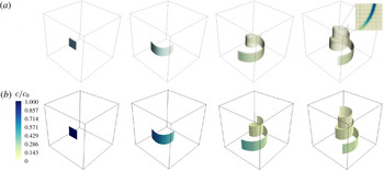
Diffusion of a square blob of scalar of side
 $\unicode[STIX]{x03C0}/2$
advected by a Batchelor vortex simulated (a) by DNS and (b) by the diffusive sheet method (DSM). Snapshots are taken at
 $t=0$
,
 $t=8$
,
 $t=24$
and
 $t=40$
. The global Péclet number
 $Pe$
based on the box size and the maximum velocity is equal to 188 400. The local Péclet number
 $Pe_{0}$
based on the initial thickness
 $s_{0}=0.05$
and the shear rate is equal to 12. In the DNS, the volume rendering uses an opacity filter evolving with time in order to emphasize the relevant concentration values. The inset in the rightmost panel shows the details of the concentration field on a horizontal cut along with the collocation points. In the DSM, the colour level represents the local concentration at the centre plane of the sheet.

Another very popular method consists of computing the evolution of the concentration field itself through direct numerical simulation (DNS) of the Navier–Stokes (for the stirring field) and Fourier (for the scalar) equations, with the appropriate space and time-step resolution (Moin & Mahesh Reference Moin and Mahesh1998). An example is shown in figure 1(a), where an initial blob of scalar rolls up around a Batchelor vortex. For such a calculation, the maximal admissible mesh size must be chosen such that the finest concentration gradients should be resolved. This is a stringent requirement in the weakly diffusive limit: in a simple flow mixing a substance with diffusivity
 $D$
, stirred at scale
 $L$
by a velocity
 $U$
, the width of the concentration gradient, also known as the Batchelor scale, is
 $L/\sqrt{Pe}$
, where the Péclet number
 $Pe=UL/D$
can be arbitrarily large. It is thus not sufficient to appropriately resolve the flow internal boundary layer
 $L/\sqrt{Re}$
, with
 $Re=UL/\unicode[STIX]{x1D708}$
the Reynolds number of the carrying fluid with viscosity
 $\unicode[STIX]{x1D708}$
, when the Schmidt number
 $Sc=\unicode[STIX]{x1D708}/D$
is larger than unity (Yeung, Donzis & Sreenivasan Reference Yeung, Donzis and Sreenivasan2005; Schwertfirm & Manhart Reference Schwertfirm and Manhart2007). In random turbulent flows, the concentration gradient presents a broad dispersion around the mean mentioned above (Schumacher, Sreenivasan & Yeung Reference Schumacher, Sreenivasan and Yeung2005), incorporating in particular gradients sharper than the mean, so that a simulation should, in principle, resolve the finest gradient of the concentration field to be faithful. The constraint of having to solve accurately for the Batchelor scale indicates that the number of points in each direction must increase as
 $N\sim Pe^{1/2}$
. The total numerical cost of a DNS is thus proportional to
 $N^{3}$
(in three dimensions) and to a factor
 $N$
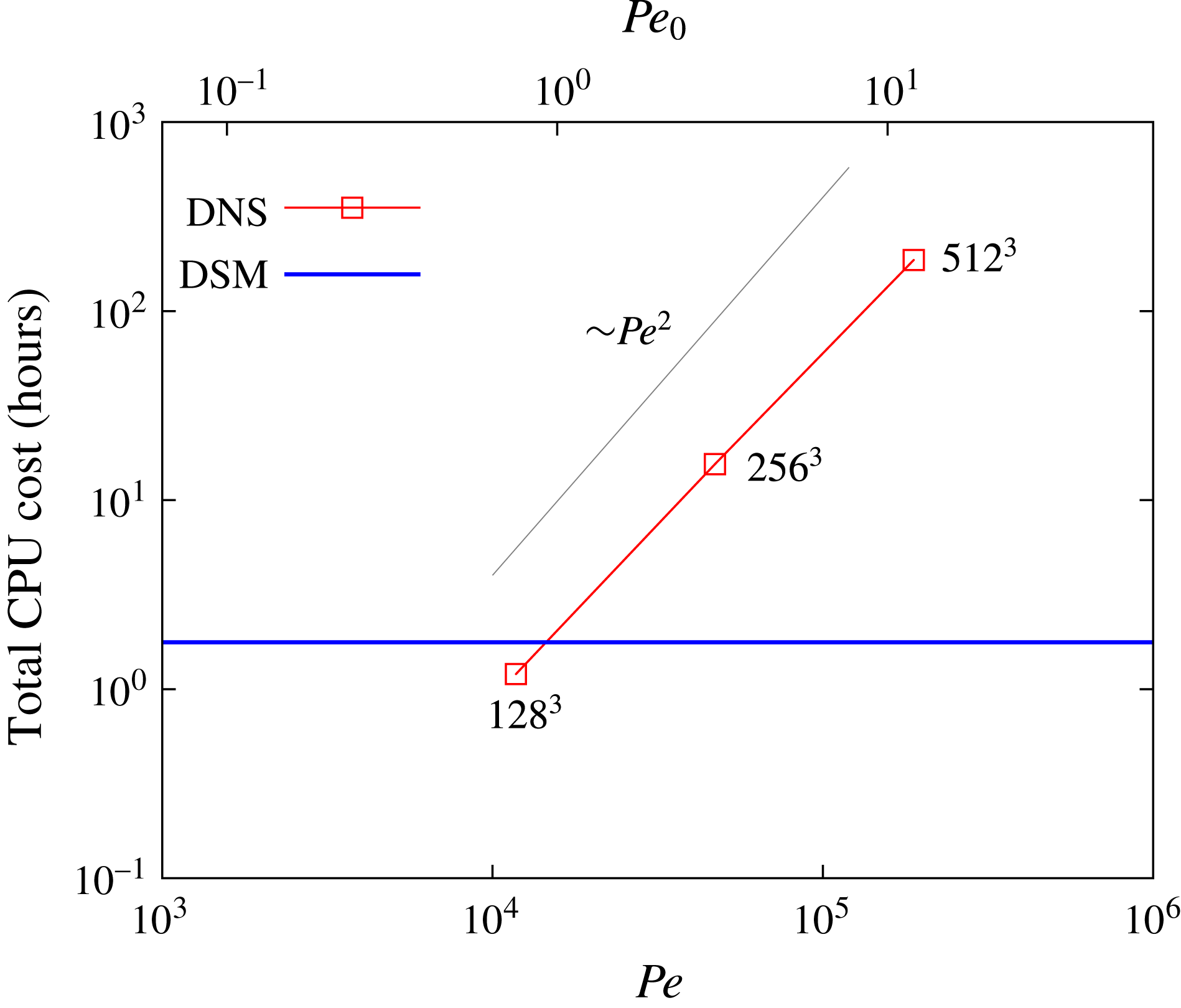
due to the decrease of the time step necessary for numerical stability. This scaling, indeed observed for the DNS calculation of a Batchelor vortex flow, as shown in figure 2, indicates that the numerical cost of a DNS scales approximately like
 $Pe^{2}$
, thus limiting its applicability to the moderate, if not low, Péclet flow regimes.
Comparison of the total numerical cost between a classical pseudospectral DNS and the new DSM. The advection of a passive scalar by a Batchelor vortex is considered (see § 2.3 for details). The numerical cost is independent of the Péclet number for the DSM whereas it scales approximately as
 $Pe^{2}$
for the DNS (the corresponding spatial resolution is indicated next to each point for reference).

Given these inherent limitations, an alternative computational method was proposed by Meunier & Villermaux (Reference Meunier and Villermaux2010), called the diffusive strip method (DSM). Instead of keeping track of the location of very many tracer particles, or solving an advection–diffusion equation for the concentration field on an extremely refined mesh, the method consists of visualizing a mixture as a set of blobs, stretched by the stirring field. The blobs are deformed kinematically by the flow, soon shaping into stretched stripes in two dimensions (Ottino Reference Ottino1989), parameterized by their local elongation. For each blob, the full advection–diffusion equation describing the dynamics of the scalar concentration is amenable, nearly rigorously (see Meunier & Villermaux Reference Meunier and Villermaux2003), to a simple diffusion equation in suitably transformed coordinates of space and time functions of the diffusivity
 $D$
and the strip elongation rate, as first exploited in this context by Ranz (Reference Ranz1979). The corresponding solution is asymptotically valid in the limit of large Péclet numbers and vanishing blob thickness with respect to the curvature radius. The method, which has a long history and a wide range of fields of interest (see the references in Meunier & Villermaux Reference Meunier and Villermaux2010), has some proximity to the flamelet representation of reactive mixtures in the combustion context (Peters Reference Peters1984), as well as direct implications for the study of mixing in particulate suspensions (Souzy et al.
Reference Souzy, Lhuissier, Villermaux and Metzger2017). Once the kinematic transport of the strip is made, the overall concentration field of the mixture is computed a posteriori, for any Péclet number
 $Pe$
, and results from a superposition principle discovered by Villermaux & Duplat (Reference Villermaux and Duplat2003), explained in detail in Duplat & Villermaux (Reference Duplat and Villermaux2008) and more recently worked out for the study of mixing by porous media (Villermaux Reference Villermaux2012a
; Le Borgne, Dentz & Villermaux Reference Le Borgne, Dentz and Villermaux2015) and for fundamental aspects of the architecture of random mixtures (Le Borgne et al.
Reference Le Borgne, Huck, Dentz and Villermaux2017). Variation of the Péclet number is thus made, with this method, at no additional cost, even for very large
 $Pe$
.
The present paper extends the two-dimensional DSM to its fully three-dimensional version which we call, by analogy, the diffusive sheet method (with, hence, the same acronym, DSM) since sheets are the three-dimensional analogues of the two-dimensional stripes (Buch Jr & Dahm Reference Buch and Dahm1996; Fountain, Khakhar & Ottino Reference Fountain, Khakhar and Ottino1998). We follow a surface advected by a three-dimensional flow, keeping track of its local expansion, thus allowing us to reconstruct the overall scalar concentration at any time, for any Péclet number. Figure 1 is a comparison of the method with a straight DNS for a simple Batchelor vortex, to be studied in detail in § 2, showing a good agreement between the two methods concerning the position of the scalar sheet. The comparative computational cost in figure 2 demonstrates the obvious advantage of the DSM over traditional DNS.
The details of the numerical method, notably the way surfaces are parameterized and refined as they are distorted by the flow, are given in § 2, where the method is also validated by a comparison with a DNS in a simple Batchelor vortex. In § 3, we study mixing in a real experiment, using a Taylor–Couette configuration whose stirring field is documented and modelled. The mixing properties of this flow, which are measured quantitatively, are inferred from its stirring kinematics and compared with the predictions from the DSM. We conclude in § 4.
2 A new method for scalar mixing in three dimensions
The mixing process of a passive-scalar substance in a prescribed flow has been modelled in many ways. The Eulerian formulation provides a full description of the evolution of a scalar concentration field through an advection–diffusion equation,
 $$\begin{eqnarray}\frac{\unicode[STIX]{x2202}c}{\unicode[STIX]{x2202}t}+\boldsymbol{v}\boldsymbol{\cdot }\unicode[STIX]{x1D735}c=D\unicode[STIX]{x0394}c,\end{eqnarray}$$
where
 $c$
is the concentration of the scalar field and
 $D$
is the diffusivity of the substance being mixed. The flow field
 $\boldsymbol{v}(\boldsymbol{x},t)$
is assumed to be known a priori and is not coupled with the evolution of
 $c$
itself, defining a passive-scalar dynamics. It is feasible to solve (2.1) with a DNS, but, as explained in § 1 and visible from figure 2, it is costly at large Péclet number.
The DSM, on the other hand, enables the study of convection–diffusion mixing problems by relying on the kinematics of the flow only. The approach consists of reducing the problem (2.1) to a simple diffusion equation in adequate rescaled coordinates, given by
 $$\begin{eqnarray}\frac{\unicode[STIX]{x2202}c}{\unicode[STIX]{x2202}\unicode[STIX]{x1D70F}}=\frac{\unicode[STIX]{x2202}^{2}c}{\unicode[STIX]{x2202}{\tilde{n}}^{2}},\end{eqnarray}$$
where
 $\unicode[STIX]{x1D70F}$
and
 ${\tilde{n}}$
are time and space variables respectively, depending on the scalar diffusivity and the topology of the velocity field, which are explicitly given below.
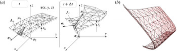
Schematic figure of the advected triangulated surface (a), where
 $s_{k}$
and
 $A_{k}$
are the striation thickness and area of a given triangle
 $k$
respectively. An arbitrary surface is chosen as initial condition (b) with homogeneous mesh triangulation (black) and flow-dependent refinement (colour). It should be noted that even though the original triangulation is evenly distributed, the refinement depends spatially on the local deformation experienced by each triangle following the flow field.

2.1 The DSM
We know (see, e.g., Batchelor Reference Batchelor1952; Cocke Reference Cocke1969; Orszag Reference Orszag1970; Girimaji & Pope Reference Girimaji and Pope1990; Duplat & Villermaux Reference Duplat and Villermaux2000) that material line elements tend to orient along the principal axis corresponding to the maximum positive strain rate (we call it
 $\unicode[STIX]{x1D6FE}$
) of the stirring field. Similarly, material area elements tend to lie in the plane of the principal strain-rate axis, whereas the principal compression direction lies perpendicular to the surface (Betchov Reference Betchov1956; Ashurst et al.
Reference Ashurst, Kerstein, Kerr and Gibson1987), an essential feature at the root of the DSM (Meunier & Villermaux Reference Meunier and Villermaux2010). When a volume of fluid is deformed, it typically stretches (more in one direction than the other; see Betchov Reference Betchov1956), and contracts in the third direction, due to incompressibility. The area
 $A_{i}(t)$
of a (non-diffusing) material element
 $i$
covering an advected surface is related to its transverse thickness
 $s_{i}(t)$
by
 $$\begin{eqnarray}s_{i}(t)=s_{i0}\frac{A_{i_{0}}}{A_{i}(t)},\end{eqnarray}$$
where
 $s_{i0}$
and
 $A_{i_{0}}$
are the initial thickness and area of element
 $i$
respectively. We will suppose that the initial distribution of scalar in the fluid bulk can be well approximated by a triangulated surface (figure 3), carrying the information on the local thickness. We now make the assumption that, in this frame of reference, the displacement field can be adequately approximated by a Taylor expansion of the flow at first order. The normal shrinking velocity is simply
 $$\begin{eqnarray}v_{n}=\frac{n}{s_{i}}\frac{\text{d}s_{i}}{\text{d}t}.\end{eqnarray}$$
This stretching dynamics produces an increasing gap of length scales between the thickness of the sheet, which diminishes with time, and the characteristic lengths along the elongating surface. Therefore, the longitudinal concentration gradients can be neglected in comparison with the normal ones (Meunier & Villermaux Reference Meunier and Villermaux2003). This allows us to rewrite the advection–diffusion equation (2.1) by neglecting the scalar gradients on the surface,
 $\unicode[STIX]{x2202}c/\unicode[STIX]{x2202}\unicode[STIX]{x1D70E}_{1}$
,
 $\unicode[STIX]{x2202}c/\unicode[STIX]{x2202}\unicode[STIX]{x1D70E}_{2}$
(see figure 3), as well as longitudinal diffusion terms as
 $$\begin{eqnarray}\frac{\unicode[STIX]{x2202}c}{\unicode[STIX]{x2202}t}+\frac{n}{s_{i}}\frac{\text{d}s_{i}}{\text{d}t}\frac{\unicode[STIX]{x2202}c}{\unicode[STIX]{x2202}n}=D\frac{\unicode[STIX]{x2202}^{2}c}{\unicode[STIX]{x2202}n^{2}}.\end{eqnarray}$$
This one-dimensional advection–diffusion equation can be further simplified by defining rescaled time and space coordinates (Ranz Reference Ranz1979),
 $$\begin{eqnarray}\unicode[STIX]{x1D70F}=D\int _{0}^{t}\frac{\text{d}t^{\prime }}{s_{i}(t^{\prime })^{2}}\quad \text{and}\quad {\tilde{n}}=\frac{n}{s_{i}(t)},\end{eqnarray}$$
thus mapping (2.5) onto the diffusion equation (2.2). For a given initial concentration profile
 $C_{0}(n)$
across the surface element, the general solution is given by
 $$\begin{eqnarray}c(\unicode[STIX]{x1D70F},{\tilde{n}})=\int _{{\tilde{n}}^{\prime }=-\infty }^{{\tilde{n}}^{\prime }=+\infty }\frac{C_{0}({\tilde{n}}^{\prime })}{\sqrt{4\unicode[STIX]{x03C0}t}}\exp \left(-\frac{({\tilde{n}}-{\tilde{n}}^{\prime })^{2}}{4\unicode[STIX]{x1D70F}}\right)\text{d}{\tilde{n}}^{\prime }.\end{eqnarray}$$
It has a simple form in the case of an initial Gaussian concentration profile
 $C_{0}({\tilde{n}})=c_{0}\exp (-{\tilde{n}}^{2})$
,
 $$\begin{eqnarray}\displaystyle & \displaystyle c(\unicode[STIX]{x1D70F},{\tilde{n}})=c_{m}\exp \left(-\frac{{\tilde{n}}^{2}}{1+4\unicode[STIX]{x1D70F}}\right), & \displaystyle\end{eqnarray}$$
 $$\begin{eqnarray}\displaystyle & \displaystyle c_{m}=\frac{c_{0}}{\sqrt{1+4\unicode[STIX]{x1D70F}}}. & \displaystyle\end{eqnarray}$$
Therefore, computation of the deformation of a scalar sheet in a fluid flow, following its local stretching rate and thickness, is sufficient to reconstruct the three-dimensional concentration field around it a posteriori, including diffusive effects. The power of this method lies in its simplicity: the computation is to be made only once and the concentration field can be obtained for any value of the diffusivity
 $D$
or initial sheet thickness
 $s_{0}$
(because they are encoded in
 ${\tilde{n}}$
and
 $\unicode[STIX]{x1D70F}$
) from a unique simulation with no additional numerical cost.
The concentration profile across a diffusing element
 $i$
paving a sheet deformed in a flow is entirely determined by its local compression state
 $s_{i}(t)$
and history (the definition of
 $\unicode[STIX]{x1D70F}$
in (2.6) involves an integral over time). These depend on the flow in particular, and several canonical examples have been considered, including random chaotic flows where
 $s_{i}(t)$
shrinks exponentially fast in time or flows where the decay is a power law (see Villermaux (Reference Villermaux2012b
) and references therein). We will be interested here in deformation fields similar to shear flows, which induce a compression as
 $$\begin{eqnarray}s_{i}(t)=\frac{s_{0}}{\sqrt{1+(\unicode[STIX]{x1D6FE}t)^{2}}},\end{eqnarray}$$
with a rate of compression
 $-\dot{s_{i}}/s_{i}$
weakening at large time as
 $t^{-1}$
. In that case, we have from (2.6)
 $$\begin{eqnarray}\displaystyle \unicode[STIX]{x1D70F}(t)=\frac{\unicode[STIX]{x1D6FE}t}{Pe_{0}}\left(1+\frac{1}{3}(\unicode[STIX]{x1D6FE}t)^{2}\right),\end{eqnarray}$$
where
 $$\begin{eqnarray}Pe_{0}=\frac{\unicode[STIX]{x1D6FE}s_{0}^{2}}{D}\end{eqnarray}$$
is the Péclet number based on the initial sheet thickness
 $s_{0}$
. Molecular diffusion alters the distribution of the concentration levels
 $c$
for times
 $\unicode[STIX]{x1D70F}$
larger than unity (Villermaux & Duplat Reference Villermaux and Duplat2003), thus defining the mixing time
 $t_{s}$
such that
 $\unicode[STIX]{x1D70F}(t_{s})=O(1)$
, providing, in the present case,
 $$\begin{eqnarray}t_{s}\sim \unicode[STIX]{x1D6FE}^{-1}Pe_{0}^{1/3}\quad \text{for}~Pe_{0}\gg 1.\end{eqnarray}$$
The maximal concentration at the centre of the sheet element given by (2.9) is constant and equal to
 $c_{0}$
for
 $t<t_{s}$
and decays as
 $$\begin{eqnarray}c_{m}\sim \unicode[STIX]{x1D70F}^{-1/2}\sim (\unicode[STIX]{x1D6FE}t)^{-3/2}\quad \text{for}~t>t_{s}.\end{eqnarray}$$
This decay law is a straightforward consequence of mass conservation
 $c_{m}\times \sqrt{Dt}\times A_{i}(t)=c_{0}\times s_{0}\times A_{i0}$
with
 $A_{i}(t)/A_{i0}=s_{0}/s_{i}(t)$
given in (2.3).
It is interesting to check that the approximation at the root of the Ranz transformation in (2.6) used by the DSM is valid. The longitudinal diffusion terms have been neglected with respect to the normal diffusion terms at the time when diffusion starts to act, i.e. at the mixing time. The ratio of these terms is proportional to
 $(\unicode[STIX]{x1D6FE}t)^{4}$
for a linear growth of the material elements, that is, equal to
 $Pe_{0}^{4/3}$
at
 $t=t_{s}$
. This ratio is equal to
 $Pe_{0}^{2}$
in the case of exponential growth of material elements. In each case, the method is thus asymptotically valid in the limit of large Péclet numbers.
2.2 Numerical implementation
A numerical code in C language was developed to simulate the advection of a prescribed sheet with the flow motion. In order to triangulate the surface and follow each triangular element, together with the information on local stretching and thickness, we have made use of the GNU Triangulated Surface (GTS) Library (Popinet Reference Popinet2010). The interest of this library lies in an efficient connection between elements such as vertices, edges and triangular faces, together with a wide set of functions that allow for fast calculation of areas, distances and normals, among others. The navigation through the hierarchy of triangles, edges and vertices pertaining to the whole surface is optimized with a tree-like structure.
A crucial point in the implementation of the DSM is the dynamic refinement of the surface. Indeed, although the initial triangulated surface is well resolved, its stretching leads to large triangles in areas where higher definition is required to properly describe the scalar distribution. Moreover, regions of the surface that display high curvature need a larger number of triangles than flat regions. The mesh-refinement process is triggered periodically (depending on the stretching experienced by the surface, every 50 time steps being typically enough for the cases considered here) by both triangle size (every triangle edge reaching a length longer than a prescribed criterion is split into two, a vertex is added at its middle point, and two new triangles are built through that new vertex) and triangle quality (a far-from-equilateral triangle is also divided to avoid a mesh predominant orientation forced by a directional stretch).
A fourth-order Runge–Kutta scheme was used to integrate the displacement of each mesh vertex with a given flow velocity field. The Courant–Friedrichs–Lewy (CFL) condition for the time step
 $\unicode[STIX]{x0394}t$
of integration is constrained by the spacing
 $l$
between contiguous vertices to be displaced with local velocity
 $\boldsymbol{v}$
, so that
 $\unicode[STIX]{x0394}t<l/|\boldsymbol{v}|$
. A surface under stretch poses a less restrictive condition as vertices move apart since mesh refinement shortens the distance between integration points. The time step is imposed such that the maximum vertex displacement between two time steps on the whole mesh is smaller than the minimum sheet edge thickness. Real flows, however, may produce material sheet folding, and seldom highly curved and/or stagnant regions where the tracers accumulate. These areas, where the DSM method breaks down, are characterized by a radius of curvature that becomes smaller than the striation thickness. In 2D, Meunier & Villermaux (Reference Meunier and Villermaux2010) found that these cusps were localized and that they did not alter the global quantities of the flow such as the probability density function and the spectra, precisely because they were less and less numerous with respect to the ever growing regular area of the sheet.
Several modifications were performed to the GTS library in order to implement the DSM: primarily, the creation of an extended triangle object to track intrinsic variables, namely the striation thickness
 $s_{i}$
and dimensionless time
 $\unicode[STIX]{x1D70F}_{i}$
. The evolution of each triangle thickness
 $s_{i}$
is computed at each time step
 $t_{n}$
from (2.3), making use of the directly measurable triangle area,
 $$\begin{eqnarray}s_{i}(t_{n})=s_{i}(t_{n-1})\frac{A_{i}(t_{n-1})}{A_{i}(t_{n})},\end{eqnarray}$$
as well as the dimensionless time (2.6),
 $$\begin{eqnarray}\unicode[STIX]{x1D70F}_{i}(t_{n})=\unicode[STIX]{x1D70F}_{i}(t_{n-1})+D\int _{t_{n-1}}^{t_{n}}\frac{\text{d}t}{s_{i}^{2}}.\end{eqnarray}$$
The concentration located at each triangular face is therefore obtained by the expression (2.9),
 $c_{mi}(t_{n})=c_{0}/\sqrt{1+4\unicode[STIX]{x1D70F}_{i}(t_{n})}$
for selected values of
 $Pe_{0}$
. A count of the number of events for values of
 $c_{m}/c_{0}$
ranging from 0 to 1 yields the distribution of maxima
 $q(c_{m})$
. Nevertheless, a more detailed distribution of the scalar concentration
 $p(c)$
can be extracted from the DSM data. Each triangular face contributes to the total distribution by a transverse Gaussian diffusive profile of concentration which peaks at the surface with a value equal to
 $c_{m}$
and reaches transverse distances of the order of
 $s_{i}\sqrt{1+4\unicode[STIX]{x1D70F}_{i}}$
(2.9). Accounting for the relative area of each triangle and the extension of their thickness, the overall concentration distribution
 $p(c)$
is constructed as the weighted sum of the whole set of elements paving the surface. Since each of them contributes by a characteristic
 $\cup$
-shaped elementary distribution (
 ${\sim}(c\sqrt{\ln [c_{M}/c]})^{-1}$
, see Meunier & Villermaux Reference Meunier and Villermaux2003), reflecting a Gaussian profile of concentration across the sheet element, we have
 $$\begin{eqnarray}\displaystyle p(c) & = & \displaystyle \mathop{\sum }_{i}p_{i}(c)\end{eqnarray}$$
 $$\begin{eqnarray}\displaystyle & {\sim} & \displaystyle \mathop{\sum }_{i}\frac{A_{i}s_{i}\sqrt{1+4\unicode[STIX]{x1D70F}_{i}}}{c\sqrt{-\log (c/c_{m})}},\end{eqnarray}$$
subjected to the normalization
 $\int p(c)\,\text{d}c=1$
.
2.3 Comparison with DNS and theoretical predictions
In order to validate the DSM and its numerical implementation, we compare it with a more conventional numerical method, namely a DNS that solves for (2.1) using an open-source pseudospectral code called SNOOPY (Lesur & Longaretti Reference Lesur and Longaretti2007). To facilitate this comparison, we consider an idealized configuration that can be explored using classical pseudospectral methods in tri-periodic domains. This allows us to reach sufficiently large Péclet numbers, which optimizes the comparison with the DSM.
For the sake of simplicity and continuity with the two-dimensional version of the DSM (Meunier & Villermaux Reference Meunier and Villermaux2010), we consider the case of a modified Batchelor vortex defined in cylindrical coordinates as
 $$\begin{eqnarray}\boldsymbol{u}=(u_{r},u_{\unicode[STIX]{x1D703}},u_{z})=\left(0,\frac{1-\text{e}^{-(r/R_{1})^{2}}}{r/R_{1}},q\text{e}^{-(r/R_{2})^{2}}\right),\end{eqnarray}$$
where
 $q$
is the axial velocity on the axis of symmetry. The classical Batchelor vortex would correspond to
 $R_{1}=R_{2}$
, with a constant axial velocity in addition to the Gaussian profile above. This flow is invariant along the vertical direction but is not periodic in the horizontal direction. Since we want to compare the DSM with a classical pseudospectral approach, the Batchelor vortex has to be regularized in order to match the tri-periodic boundary conditions. This is achieved by multiplying the velocity components by a two-dimensional Tukey window localized on the vertical sides of a cubic domain of side
 $L=2\unicode[STIX]{x03C0}$
centred around the origin. For instance, in order to enforce periodicity in the
 $x$
direction, the velocity components are multiplied by the following window function:
 $$\begin{eqnarray}f(x)=\left\{\begin{array}{@{}ll@{}}\displaystyle \frac{1}{2}\left(1+\cos \left(\unicode[STIX]{x03C0}\frac{-\unicode[STIX]{x03C0}-x+\unicode[STIX]{x1D716}}{\unicode[STIX]{x1D716}}\right)\right)\quad & \text{if}~x\in [-\unicode[STIX]{x03C0},-\unicode[STIX]{x03C0}+\unicode[STIX]{x1D716}],\\ 1\quad & \text{if}~x\in [-\unicode[STIX]{x03C0}+\unicode[STIX]{x1D716},\unicode[STIX]{x03C0}-\unicode[STIX]{x1D716}],\\ \displaystyle \frac{1}{2}\left(1+\cos \left(\unicode[STIX]{x03C0}\frac{\unicode[STIX]{x03C0}-x+\unicode[STIX]{x1D716}}{\unicode[STIX]{x1D716}}\right)\right)\quad & \text{if}~x\in [\unicode[STIX]{x03C0}-\unicode[STIX]{x1D716},\unicode[STIX]{x03C0}],\end{array}\right.\end{eqnarray}$$
where
 $\unicode[STIX]{x1D716}$
is a small constant, typically
 $\unicode[STIX]{x1D716}=10^{-1}$
. The resulting flow is
 $2\unicode[STIX]{x03C0}$
-periodic in both horizontal directions and exactly corresponds to the Batchelor vortex, apart from a very thin region close to the vertical boundaries of the cubic domain. In the following, the concentration is non-zero only in the central part of the vortex, ensuring that our localized regularization does not affect the results in the bulk of the vortex.
The initial condition for the passive scalar is given by
 $$\begin{eqnarray}c(x,y,z,t=0)=\left\{\begin{array}{@{}ll@{}}\text{e}^{-(y/s_{0})^{2}}\quad & \displaystyle \text{if}~x\in \left[-\frac{3\unicode[STIX]{x03C0}}{4},\frac{-\unicode[STIX]{x03C0}}{4}\right],z\in \left[\frac{-5\unicode[STIX]{x03C0}}{6},\frac{-\unicode[STIX]{x03C0}}{3}\right],\\ 0\quad & \text{elsewhere},\end{array}\right.\end{eqnarray}$$
where
 $s_{0}$
is the initial thickness of the scalar sheet. Although this exact initial condition was imposed in the DSM calculations, a regularization of the edges and corners of the initial sheet is required in DNS in order to build a continuous three-dimensional scalar field. This is achieved by using the same Gaussian profile in all directions around the sheet border.
From a numerical point of view, the scalar is decomposed onto
 $N$
Fourier modes in each direction. The diffusive term in (2.1) is solved implicitly using exponential factors whereas the advection term is solved explicitly using a fourth-order Runge–Kutta scheme. The solution is fully dealiased using the
 $2/3$
truncation method. The numerical resolution of the DNS depends on the Batchelor scale, defined as the length scale where diffusion balances stretching by the flow. In the following, we simply assume that a DNS of (2.1) requires a grid size of the order of the Batchelor scale.
The results shown in figures 1 and 4 were obtained for the set of parameters
 $R_{1}=0.3$
,
 $R_{2}=0.9$
,
 $q=0.2$
,
 $s_{0}=0.05$
and
 $D=1/30\,000$
. This corresponds to a global Péclet number of
 $Pe=UL/D\approx 188\,400$
using
 $U\approx 1$
and
 $L=2\unicode[STIX]{x03C0}$
. The local Péclet number, relevant for the DSM, is
 $Pe_{0}=\unicode[STIX]{x1D6FE}s_{0}^{2}/D\approx 12$
using
 $\unicode[STIX]{x1D6FE}\approx U/L\approx 0.16$
. The Batchelor scale (Batchelor (Reference Batchelor1959); see also Villermaux (Reference Villermaux2012a
) for an adaptation to a decaying stretching rate) can be estimated by
 $\ell _{B}=\sqrt{D/\unicode[STIX]{x1D6FE}}\approx 0.015$
, which imposes a resolution of at least 512 Fourier modes in each direction so that
 $\ell _{B}\approx 1.2\,\text{d}x$
(
 $\text{d}x$
being the grid size). We study the evolution of the scalar sheet up to
 $t=40$
. Figure 1 shows isocontours of the scalar field at the particular value
 $c/c_{0}=10^{-3}$
for different times together with the DSM zero-thickness surface and local maximum concentration. The DSM simulation is run for 25 000 time steps, the final surface is composed of 77 688 triangles and the time step, which varies in time according to the mesh refinement and the velocity field, ranges from
 $10^{-2}$
to
 $10^{-4}$
. The total area grows linearly with time; therefore, upon mesh refinement, the number of triangles used to describe the surface grows linearly with time too. The temporal evolution of the maximum concentration in the field,
 $c_{M}=\max (c_{mi})$
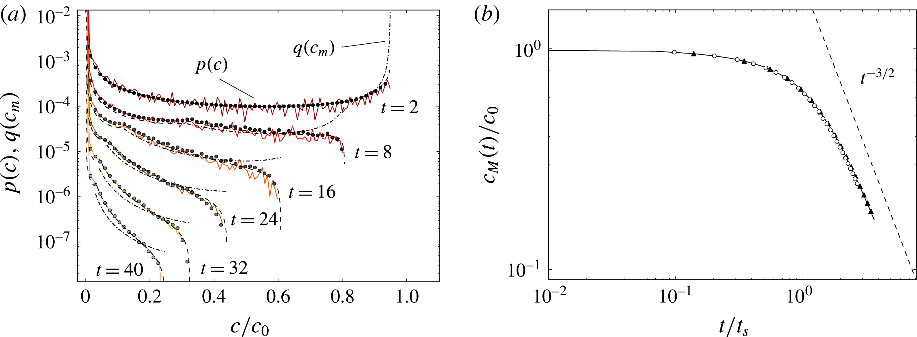
, is shown in figure 4(b), comparing the data obtained with the DNS (dots), the DSM (solid line) and the theoretical prediction (dot-dashed),
 $$\begin{eqnarray}c_{M}=\max \left(\frac{c_{0}}{\sqrt{1+4\unicode[STIX]{x1D70F}(r)}}\right),\quad \text{where}~\unicode[STIX]{x1D70F}(r)=t\frac{D}{{s_{0}}^{2}}+t^{3}\frac{D\unicode[STIX]{x1D6E4}^{2}}{3\unicode[STIX]{x03C0}^{2}r^{4}{s_{0}}^{2}},\end{eqnarray}$$
with
 $\unicode[STIX]{x1D6E4}=2\unicode[STIX]{x03C0}R_{1}$
the circulation of the vortex and
 $r$
the radial position of the scalar. For the problem considered here, the mixing time (2.13) is approximately
 $t_{s}\approx 14$
and the expected decay
 $c_{M}\sim t^{-3/2}$
for
 $t>t_{s}$
is observed.
(a) The probability density function of concentrations
 $p(c)$
at successive times given by the DSM (white circles), the DNS computation (solid colour lines) and the theoretical prediction (black circles) for
 $s_{0}=0.05$
,
 $D=30\,000^{-1}$
and
 $\unicode[STIX]{x1D6FE}=0.16$
, and thus
 $Pe_{0}=\unicode[STIX]{x1D6FE}s_{0}^{2}/D\approx 12$
. The theoretical prediction of
 $q(c_{m})$
(dot-dashed) is added for the sake of completeness. The distributions at different times have been shifted downwards for clarity. (b) The temporal evolution of the concentration maximum computed with the DSM (solid line), DNS (white circles) and the theoretical evolution for the Batchelor vortex (black triangles).

The probability density function
 $p(c)$
for this Batchelor vortex is computed at different times from the DNS data and shown in figure 4(a). The DSM prediction from (2.18) is in excellent agreement with it, as well as with the expected distribution of maximal concentrations
 $q(c_{m})\sim 1/(\text{d}c_{m}/\text{d}r)$
and concentration distribution
 $p(c)$
, which are
 $$\begin{eqnarray}\displaystyle & \displaystyle q(c_{m})=\frac{t^{3/4}{s_{0}}^{2}}{(-({c_{m}}^{2}-1){s_{0}}^{2}-4tD{c_{m}}^{2})^{5/4}}\sqrt{\frac{\unicode[STIX]{x1D6E4}}{2\unicode[STIX]{x03C0}}}\left(\frac{D}{3}\right)^{1/4}\sqrt{-\frac{2}{c_{m}}-\frac{3}{4}\frac{({c_{m}}^{2}-1){s_{0}}^{2}}{tD{c_{m}}^{3}}},\qquad & \displaystyle\end{eqnarray}$$
 $$\begin{eqnarray}\displaystyle & \displaystyle p(c)=\int _{r_{min}}^{r_{max}}\frac{\sqrt{1+4\unicode[STIX]{x1D70F}(r)}}{c\sqrt{-\log (c\sqrt{1+4\unicode[STIX]{x1D70F}(r)})}}\,\text{d}r,\qquad & \displaystyle\end{eqnarray}$$
where
 $r_{min}=\unicode[STIX]{x03C0}/4$
and
 $r_{max}=3\unicode[STIX]{x03C0}/4$
. Initially,
 $p(c)$
displays a
 $\cup$
shape (the signature in concentration space of the spatial Gaussian profile), implying large values of the initial concentration, peaking at
 $c/c_{0}=1$
and
 $c/c_{0}=0$
. Progressively, the large concentrations are transported towards lower levels, which sit on the most stretched area and are thus proportionally more numerous, therefore modifying the shape of
 $p(c)$
into a globally decaying distribution in
 $c$
, the most probable levels being close to
 $c=0$
at maximal dilution.
Let us now discuss the relative numerical cost between the two methods. The DNS is run until
 $t=40$
, which corresponds to 6692 iterations with a typical time step of
 $\text{d}t=6\times 10^{-3}$
fixed by the CFL condition associated with the explicit treatment of the advection term. Using 16 Intel Xeon processors and a parallelization using Message Passing Interface, the simulation took approximately 11.5 h, for a total CPU cost of approximately 187 h (which does not include the additional time spent writing outputs). This has to be compared with the DSM numerical cost, which is approximately 1.5 h on one single processor of a personal laptop. In addition, it is straightforward to change the Péclet number for the DSM since it corresponds to changing the diffusive kernel while keeping the same Lagrangian advection of the sheet. On the contrary, a new simulation must be run from scratch to change the Péclet number in a DNS. Additionally, any increase of the Péclet number increases the DNS cost accordingly: the spatial resolution is fixed by the Batchelor scale
 $\ell _{B}=\sqrt{D/\unicode[STIX]{x1D6FE}}\sim L/Pe^{1/2}$
. Let us assume that we fix the spatial resolution according to
 $\ell _{B}=\text{d}x=L/N$
, where
 $\text{d}x$
is the grid size. The total numerical cost of a DNS scales approximately as
 $N^{4}$
(a factor
 $N^{3}$
is due to the increase in spatial resolution in each direction and a factor
 $N$
is due to the decrease in time step associated with the CFL condition, increasing the number of iterations required to reach a given physical time). This means that the computational cost of a DNS goes like
 $Pe^{2}$
, as shown in figure 2, which limits its applicability to low Péclet numbers only. The DSM cost, however, is independent of the Péclet number and therefore out-scales any classical Eulerian grid-based method in the limit of large Péclet number.
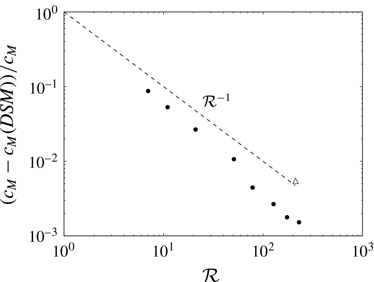
The spatial convergence of the DSM simulations has been tested by gradually increasing the number of triangles with a constant time step for all cases and dynamical refinement switched off. We recall that the temporal integration is based on a fourth-order Runge–Kutta scheme. Figure 5 shows that the relative error between the quasianalytical solution and the DSM is typically below 1 %. The method is of order one with respect to the parameter
 ${\mathcal{R}}=\sqrt{N}$
corresponding to the inverse of the mesh size. It is clear that a better convergence could be obtained by using optimized parameterizations of the surface as in Branicki & Wiggins (Reference Branicki and Wiggins2009). Furthermore, the description of invariant manifolds in 3D has been extensively studied recently (see the review by Krauskopf et al.
Reference Krauskopf, Osinga, Doedel, Henderson, Guckenheimer, Vladimirsky, Dellnitz and Junge2005), leading to various techniques that might be useful for the advection of the sheet in the DSM. However, it should be noted that the error is already extremely small, with a moderate number of flat triangles showing that the DSM is extremely promising.
The relative error on the maximum concentration at time
 $t=40$
for the case of the Batchelor vortex as a function of the resolution parameter
 ${\mathcal{R}}=\sqrt{N}$
, where
 $N$
is the number of triangles. The white triangle shows the relative error for the actual simulation discussed in the paper where dynamical refinement and adaptive time steps are used.

2.4 Reconstruction of the scalar field
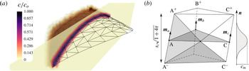
The information confined at the surface of an advected sheet in the DSM suffices to infer the local structure of the mixture (maximal concentration and sheet thickness) as long as the sheet does not fold onto itself. However, when two subparts of the sheet are brought close by so that their diffuse Gaussian concentration boundaries overlap (a process called aggregation; see Duplat & Villermaux Reference Duplat and Villermaux2008), the local maximal concentration is not equal to the maximal concentration of each subpart. In that case, a full 3D reconstruction of the scalar field is necessary, as shown in figure 6(a).
(a) Scalar reconstruction in three dimensions around the simulated 3D-DSM triangulated surface and cut-plane depicting the concentration level for a coarse mesh and a moderate
 $Pe$
for the sake of visualization. (b) Discretized coordinates inside truncated volumes of triangular base
 $\widehat{\text{ABC}}$
are filled with concentration levels defined by the Gaussian profile in the transverse direction
 $\boldsymbol{n}$
.

A three-dimensional reconstruction of the spatial distribution of scalar is performed in the following way. Once the elongation of each triangle is computed, the concentration level
 $c_{m}=c_{0}/\sqrt{1+4\unicode[STIX]{x1D70F}_{i}}$
at the mid-plane of the virtual surface is obtained. This is the maximum value of the transverse diffusional Gaussian profile, which depends on time and on the prescribed Péclet number (see (2.9)). The concentration decays with the distance from the sheet mid-plane, as shown in figure 6(b). Therefore, a concentration value, coming from each triangle, is set for each coordinate in the three-dimensionally discretized surrounding space through the relative position to each triangle. The procedure considers truncated volumes around each triangular face such that two neighbouring triangles do not contribute to the same space and nor are vacuum volumes left in between. For each triangle, every vertex A, B and C is shifted in the direction resulting from the sum of the normals of all of the triangles pertaining to that specific vertex
 $\boldsymbol{m}_{a}$
,
 $\boldsymbol{m}_{b}$
,
 $\boldsymbol{m}_{c}$
, to yield A+, B+ and C+, as shown in figure 6(b), and in the opposite direction to yield A-, B- and C-. The distance that places these sets apart is the thickness of the diffusive profile
 $s_{i}\sqrt{1+4\unicode[STIX]{x1D70F}_{i}}$
. The truncated volume is then enclosed by a constructed set of four triangles for each lateral face (as shown in the figure, A+C+C-A-) and the top and bottom covers.
The algorithm to reconstruct the concentration field makes use of the GTS library to identify the points lying inside each volume and then provides a concentration value depending on the distance from the mid-plane
 $\widehat{\text{ABC}}$
through the Gaussian profile and on the calculated
 $c_{m}$
of that triangle with the DSM, by summation. Figure 6(a) shows a scalar reconstruction around a given triangulated surface of 200 elements (black lines) and a cut-plane view across one section of it (grey plane with isocontours). The algorithm has been used with a three-dimensional discretization of
 $100^{3}$
points in a cube containing the whole surface at
 $t=2$
s for
 $Pe_{0}=5000$
.
This procedure eliminates the multiple contributions of a direct transverse filling of the concentration level to points near curved regions of the surface. Nevertheless, it allows for the aggregation process (the concentration sums) to be well treated since non-neighbouring triangles sitting in different regions of a folded surface could contribute from opposite sides to overlapping volumes between two scalar sheets when the distance between those sheets is smaller than the thickness
 $s_{i}\sqrt{1+4\unicode[STIX]{x1D70F}}$
.
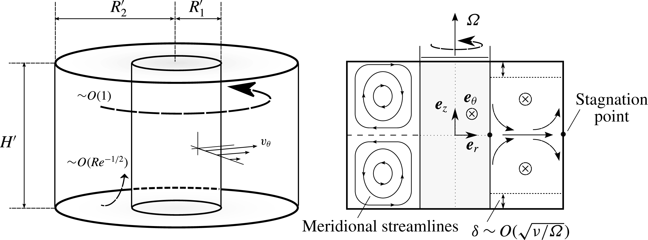
Schematic view of the Taylor–Couette configuration. A primary azimuthal flow
 $v_{\unicode[STIX]{x1D703}}$
of order 1 is generated by the inner rotating cylinder (
 $r=R_{1}^{\prime }$
). The presence of viscous boundary layers at the top and bottom induces a secondary circulation of order
 $Re^{-1/2}$
in the meridian plane, also known as Ekman pumping.

3 A real Taylor–Couette flow
We now investigate the capabilities of the DSM in representing a mixing experiment in a real flow, at much higher Péclet number than those reachable by DNS. In order to model the velocity field correctly and simply, the flow is, on purpose, chosen axisymmetric and stationary. The well-known Taylor–Couette configuration formed by the gap between two concentric cylinders is an excellent candidate due to its experimental and numerical simplicity.
3.1 Experimental set-up
A small solid cylinder of radius
 $R_{1}^{\prime }=2$
cm is located concentrically in a larger glass cylinder of radius
 $R_{2}^{\prime }=5$
cm (see figure 7). The flow under study is located between the two cylinders and delimited vertically by a flat bottom and a flat PMMA transparent top at a height
 $H^{\prime }=6$
cm. The inner solid cylinder is rotated using a brushless motor at an angular velocity
 $\unicode[STIX]{x1D6FA}$
equal to 1.5 or
 $3~\text{rad}~\text{s}^{-1}$
while the outer cylinder is kept motionless. The working fluid is made of a mixture of water and a volume fraction of 10 % of UCON oil (which is approximately 40 000 times more viscous than water at room temperature (UCON 75-H-90,000, available from DOW Company, Michigan, USA)). This working mixture has a viscosity five times larger than the viscosity of water, which prevents the appearance of time-dependent centrifugal instabilities. This property also has the advantage of decreasing the diffusion coefficient
 $D$
of the working fluid (Sutherland Reference Sutherland1905) and hence increasing the Péclet number by a factor of 5. The diffusion coefficient of fluorescein in this mixture is equal to
 $10^{-10}~\text{m}^{2}~\text{s}^{-1}$
.
The inner-cylinder characteristic length
 $R_{1}^{\prime }$
and rotation-associated time
 $\unicode[STIX]{x1D6FA}^{-1}$
are chosen to non-dimensionalize the problem. The non-dimensional parameters are the dimensionalized outer cylinder
 $R=R_{2}^{\prime }/R_{1}^{\prime }=2.5$
, the aspect ratio
 $H=H^{\prime }/R_{1}^{\prime }=3$
, the Reynolds number
 $Re=\unicode[STIX]{x1D6FA}{R_{1}^{\prime }}^{2}/\unicode[STIX]{x1D708}$
(which is equal to 120 and 240 at
 $\unicode[STIX]{x1D6FA}=1.5$
and
 $3~\text{rad}~\text{s}^{-1}$
respectively) and the Péclet number
 $Pe=\unicode[STIX]{x1D6FA}{R_{1}^{\prime }}^{2}/\unicode[STIX]{x1D708}$
(equal to
 $6\times 10^{6}$
and
 $12\times 10^{6}$
at
 $\unicode[STIX]{x1D6FA}=1.5$
and
 $3~\text{rad}~\text{s}^{-1}$
respectively, out of reach from DNS).
Two different visualization methods are used to characterize the mixing induced by this flow. First, an illumination in volume provided by an LED strip wound around the outer cylinder is used, which allows for qualitative top-view visualizations. This strip superimposes RGB LEDs such that the emitted light can be tuned in colour and intensity in order to excite fluorescein and/or rhodamine. Second, a 1.5 W blue laser (488 nm) is used to produce a luminous meridian sheet of 0.5 mm thickness. Side view visualizations permit quantitative measurement of the light intensity which has been calibrated with respect to the concentration in fluorescein. Both imaging techniques are optimized by painting the bottom disk and the inner cylinder black to avoid undesired reflection. Images are recorded using a sensitive 8 bit camera.
3.2 Laminar flow field
The rotation of the inner cylinder at
 $\unicode[STIX]{x1D6FA}$
induces an azimuthal velocity
 $v_{\unicode[STIX]{x1D703}}$
, as shown in figure 7. This flow would be invariant along the axial coordinate
 $z$
for an infinite cylinder height
 $H^{\prime }$
since the experiments were carried out at sufficiently low Reynolds number to prevent centrifugal instabilities. However, the presence of the top and bottom end plates induces a strong Ekman pumping, leading to a meridional recirculation shown schematically in figure 7. These two torus-like vortices break the
 $z$
-invariance of the azimuthal velocity while preserving the axisymmetry and the stationarity of the flow. This 3D viscous flow is not known theoretically and it has thus been measured experimentally and simulated numerically. It has then been fitted by an analytical model which will be used as an input for the DSM simulations.
3.2.1 Particle image velocimetry (PIV) measurements
In order to measure the velocity in a meridional plane, the flow was seeded with small buoyant particles of diameter
 $100~\unicode[STIX]{x03BC}\text{m}$
and the meridional laser sheet was thickened to 3 mm to prevent particles from leaving the sheet during the time
 $\unicode[STIX]{x0394}t=0.04$
s between two images. Images were first recorded from a side view orthogonal to the meridional laser sheet and treated using an intercorrelation PIV algorithm (Meunier & Leweke Reference Meunier and Leweke2003). This leads to instantaneous meridional velocity fields
 $(v_{r},v_{z})$
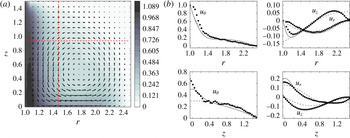
, which are then averaged over 100 realizations of the fields. Figure 8(a) shows the upper half of the meridional plane, where the torus-like vortex is clearly visible. The third component of the velocity,
 $v_{\unicode[STIX]{x1D703}}$
, can also be obtained by recording images with an angle
 $\unicode[STIX]{x1D6FC}\approx 15^{\circ }$
with respect to the normal of the laser sheet. This stereoscopic PIV measurement gives a horizontal velocity component equal to
 $\cos (\unicode[STIX]{x1D6FC})v_{r}+\sin (\unicode[STIX]{x1D6FC})v_{\unicode[STIX]{x1D703}}$
, from which the azimuthal component
 $v_{\unicode[STIX]{x1D703}}$
can be extracted by comparison with the previous (orthogonal) measurement. This azimuthal velocity is plotted as a colour scale in figure 8(a). It clearly shows that the strong azimuthal velocity located close to the inner cylinder is advected by the meridional flow at mid-height towards the outer cylinder. It should be noted that there is a (weakly visible) velocity discontinuity at the top left corner due to the sliding of the rotating inner cylinder along the motionless top end plate.
Particle image velocimetry measurements of the Taylor–Couette flow at
 $Re=120$
. (a) The vector field (
 $u_{r}$
,
 $u_{z}$
) is superimposed on the azimuthal velocity
 $u_{\unicode[STIX]{x1D703}}$
plotted as grey scale. (b) Experimental velocity profiles at
 $z=0.95$
(top) and
 $r=1.5$
(bottom) are plotted as symbols and compared with numerical simulations (solid lines) and analytic expressions (dashed lines) given by (3.2).

Two different velocity profiles are extracted from this experimental velocity field and compared with axisymmetric numerical simulations obtained with a finite element code. There is an excellent agreement between the experimental results (symbols) and the numerical results (solid lines) except for a 20 % discrepancy close to the inner cylinder for the radial velocity and at mid-height for the axial profile. This is probably due to the strong azimuthal velocity in these regions which creates a loss of particles between the two images despite the large thickness of the laser sheet during the PIV measurement.
3.2.2 Analytical field approximation
Analytical expressions are used to fit the velocity components measured in the previous section. The azimuthal velocity can be chosen independently of the radial and axial velocities, these two being linked by continuity as
 $$\begin{eqnarray}\frac{1}{r}\frac{\unicode[STIX]{x2202}(ru_{r})}{\unicode[STIX]{x2202}r}+\frac{\unicode[STIX]{x2202}u_{z}}{\unicode[STIX]{x2202}z}=0.\end{eqnarray}$$
This constraint is easily fulfilled by assuming that they derive from a stream function
 $\unicode[STIX]{x1D6F9}(r,z)$
as
 $u_{r}=-(1/r)(\unicode[STIX]{x2202}\unicode[STIX]{x1D6F9}/\unicode[STIX]{x2202}z),u_{z}=(1/r)(\unicode[STIX]{x2202}\unicode[STIX]{x1D6F9}/\unicode[STIX]{x2202}r)$
. This stream function is taken as a sum of Fourier modes whose parity is chosen in order to respect the impermeable boundary conditions. For two Fourier modes, this leads to
 $$\begin{eqnarray}\left.\!\begin{array}{@{}c@{}}\displaystyle u_{r}=\frac{1}{r}\frac{2\unicode[STIX]{x03C0}K}{H}\left[\sin \left(\frac{\unicode[STIX]{x03C0}(r-1)}{R-1}\right)\right]\left[\cos \left(\frac{2\unicode[STIX]{x03C0}z}{H}\right)+a\cos \left(\frac{4\unicode[STIX]{x03C0}z}{H}\right)\right],\\ \displaystyle u_{\unicode[STIX]{x1D703}}=\exp \!\left[-\frac{c_{1}(r-1)}{\tanh (c_{2}(H/2-z))}-\frac{c_{1}(r-1)}{\tanh (c_{2}(H/2+z))}\right]\!+c_{3}\sin ^{2}\!\left(\frac{\unicode[STIX]{x03C0}(r-1)}{R-1}\right)\!\!\left(\!1-\frac{4z^{2}}{H^{2}}\right)\!,\\ \displaystyle u_{z}=\frac{-1}{r}\frac{\unicode[STIX]{x03C0}K}{R-1}\left[\cos \left(\frac{\unicode[STIX]{x03C0}(r-1)}{R-1}\right)\right]\left[\sin \left(\frac{2\unicode[STIX]{x03C0}z}{H}\right)+\frac{a}{2}\sin \left(\frac{4\unicode[STIX]{x03C0}z}{H}\right)\right],\end{array}\right\}\end{eqnarray}$$
where
 $K$
and
 $a$
allow the radial and vertical velocity to be fitted. The azimuthal velocity
 $u_{\unicode[STIX]{x1D703}}$
is sought as the sum of two terms. The first term (containing two fitting constants
 $c_{1}$
and
 $c_{2}$
) models the singularities at the top and bottom inner corners. The second term (with amplitude
 $c_{3}$
) models the bulk flow. These expressions are plotted as dashed lines in figure 8(b) and compared with the PIV measurements (dots) and the numerical simulations (solid lines) with
 $K=0.95$
,
 $a=0.4$
,
 $c_{1}=1.8$
,
 $c_{2}=1.2$
and
 $c_{3}=0.17$
. There is a good agreement between the analytical model and the numerical solution in the bulk of the flow. The model is not perfectly tuned inside the boundary layers (see, for example, the divergence of
 $u_{z}$
in the radial profile for
 $r^{\prime }<2.5$
cm) since the model is chosen with slip boundary conditions for simplicity. However, these simple expressions are sufficient to study the dynamics of the scalar since it is injected and remains far from the boundary layers. This analytical flow field is used in the following as an input for the DSM simulations.
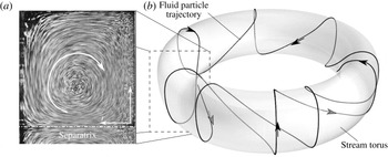
(a) Averaged stack of particle images in a meridional section, revealing the meridional streamlines. (b) Schematic drawing of a 3D streamline and its stream torus.

3.3 Topology and dynamics of the scalar
The structure of the streamlines obviously reflects the axisymmetry of the flow. The projection of the streamlines on a meridional plane is made of concentric closed curves due to the meridional circulation, as revealed by the stack of particle images of figure 9(a). The 3D streamlines lie on the tori obtained by revolving these closed curves around the cylinder axis, as schematically shown in figure 9(b). Each streamline looks like a helix wrapped around the inner cylinder. However, this helix is asymmetric since the azimuthal velocity is smaller at the outer top side of the torus than at the inner bottom side. It should be noted that these streamlines do not need to be closed curves since the period of rotation in the meridional plane and around the axis may not be commensurate.
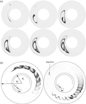
Top views of the Taylor–Couette cell under global LED illumination. (a) Raw images showing the successive deformation of a fluorescein blob into a helical strip just after injection at radius 4 cm and after 2, 4, 6, 8 and 10 turns in the cell for a rotation rate of
 $1.5~\text{rad}~\text{s}^{-1}$
and
 $Re=120$
. (b) Top-view images of a developed fluorescein strip after several turning periods for
 $Re=120$
(left) and
 $Re=240$
(right).

This helical topology is indeed observed experimentally on injecting a scalar blob into the bulk of the flow (at approximately half a radius below the top end plate). Figure 10 shows the structure of the scalar illuminated in volume for different blob injection locations and Reynolds numbers. The scalar progressively shapes into a helical strip wrapped around the cylinder axis. The helix is also asymmetric and its amplitude is larger when the injection location is closer to the cell wall boundaries.
The initial scalar blob, because it is a blob and not a point, is not located on a single torus: it ranges from a small torus to a large torus, which have different azimuthal velocities. At the smaller Reynolds number (
 $\unicode[STIX]{x1D6FA}=1.5~\text{rad}~\text{s}^{-1}$
), the smaller torus is advected faster than the larger torus, such that the head of the spiral has a smaller diameter than its tail. It is surprising to see that this phenomenon is reversed at the larger Reynolds number (
 $\unicode[STIX]{x1D6FA}=3~\text{rad}~\text{s}^{-1}$
), where the head has a larger diameter than the tail. This is due to the fact that a strong azimuthal velocity is present in the viscous boundary layers which become thinner at large Reynolds number and cannot reach the inner part of the helix. This highlights the fact that the structure of the scalar is sensitive to the Reynolds number via the position of the meridional streamlines with respect to the azimuthal velocity field.
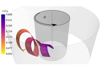
Numerical simulation of an injected blob at flow conditions given by
 $Re=120$
,
 $Pe=6\times 10^{6}$
. A ribbon-like surface, as observed in the experiments, is obtained through the numerical advection of the vertex positions at time 1.5
 $t_{s}$
. The initial thickness of the sheet is taken such that the local Péclet number is equal to
 $Pe_{0}=\unicode[STIX]{x1D6FA}s_{0}^{2}/D=5000$
.

The structure of the scalar is then checked numerically using the DSM. The velocity field is prescribed analytically for the low-Reynolds-number flow (
 $\unicode[STIX]{x1D6FA}=1.5~\text{rad}~\text{s}^{-1}$
) by (3.2), with
 $K=0.95$
,
 $a=0.4$
,
 $c_{1}=1.8$
,
 $c_{2}=1.2$
and
 $c_{3}=0.17$
. The initial sheet of scalar is located at
 $r\simeq 1.45$
,
 $z\simeq 0.4$
with a virtual thickness equal to
 $s_{0}=0.7$
mm. Figure 11 shows the position of the scalar sheet at time
 $t\simeq 42$
s. The sheet indeed rolls up into a helix where the head has a smaller diameter than the tail. The helix presents approximately three pitches and the pitch is equal to 0.43, which is in good agreement with the experiment. The location of the sheet could have been predicted by a classical Lagrangian method. However, the DSM simulations give much more information, as will be shown below.
3.4 Maximum scalar concentration
For any distorted state of the scalar sheet, the DSM predicts the concentration field structure around it. Figure 11 shows the maximum concentration
 $c_{m}$
along the sheet, no longer equal to its initial value
 $c_{0}$
at that instant of time. The maximum of the scalar has been reduced by approximately 40 % at the head of the helix. At the tail of the spiral, the scalar has been reduced by a factor of 10, which indicates that the stretching has been larger there, where the diameter of the helix is larger than at the tail.
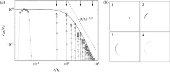
(a) The temporal evolution of the maximum concentration obtained experimentally (round symbols) and numerically (solid line) for
 $Re=120$
. Time is scaled by the longest mixing time
 $t_{s}=35~\text{s}$
given by the less stretched regions. The numerical prediction is computed with
 $c_{M}=\max [\text{erf}(1/4\sqrt{\unicode[STIX]{x1D70F}})]$
for a characteristic top-hat function of the diffusive profile (see (3.3)). (b) Experimental visualization of the scalar blob within the meridional laser sheet at four different times marked by arrows in (a).

On the experimental side, the laser-induced fluorescence technique gives quantitative measurements of the fluorescein concentration
 $c$
in a meridional section. Such visualizations are shown in figure 12(b) at the exact time when the stretched blob reaches this meridional section. In the first and second images (obtained after one and two rotations around the cylinder axis respectively), the concentration is almost equal to the initial concentration. However, in the third and fourth images, the blob has been sufficiently stretched for diffusion to set in and decrease the concentration levels.
The global maximum concentration of the scalar,
 $c_{M}=\max (c_{m})$
, defined in (2.22), can be measured both from the DSM and from the experiment. A slight modification to match the injection condition of the blob in the experiment is, however, in order. The blob is initially segregated from the diluting environment, and in that case the initial concentration profile across the deformed blob is not a Gaussian as used before for numerical convenience, but a top-hat profile, for which, in place of (2.9), we have (Villermaux & Duplat Reference Villermaux and Duplat2003)
 $$\begin{eqnarray}c_{m}=c_{0}\,\text{erf}(1/4\sqrt{\unicode[STIX]{x1D70F}}),\end{eqnarray}$$
with no other consequence on the trends and scaling dependences but slight quantitative differences with (2.9). The temporal evolution of
 $c_{M}$
is plotted in figure 12(a) as a solid line and compared with the direct measurements. Unlike the numerical simulations, the experimental measurements do not give the full three-dimensional concentration field, so that
 $c_{M}$
is only obtained at discrete times when the blob passes through the laser sheet (distinguished as grey symbols). The maximal concentration remains constant up to a mixing time
 $t_{s}$
and then decreases as
 $t^{-3/2}$
. This temporal evolution is observed for any triangular element of the sheet in the DSM and it is only the mixing time that varies from one triangle to another, depending on the local stretching. The maximal concentration
 $c_{M}$
is found on the triangle that has been the least stretched, and that has therefore the longest mixing time
 $t_{s}$
.
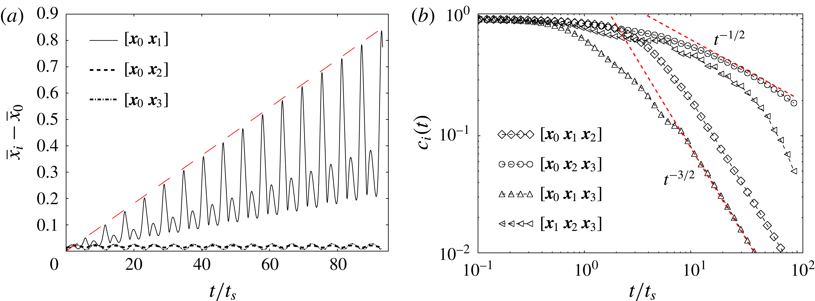
(a) The temporal evolution of the distance between two nearby tracers initially aligned in the
 $r$
direction (solid line), in the azimuthal direction (dashed line) and in the axial direction (dotted line). The long-dashed line is drawn to point out the linear growth of
 $[\boldsymbol{x}_{0}\boldsymbol{x}_{1}]$
. (b) The scalar concentration decay for the four triangular surface elements based on the four tracers used in (a). The local Péclet number
 $Pe_{0}=\unicode[STIX]{x1D6FA}s_{0}^{2}/D$
based on the initial thickness
 $s_{0}$
is taken equal to 100.

The temporal decay
 $c_{m}\sim (t/t_{s})^{-3/2}$
observed all along the sheet for
 $t>t_{s}$
indicates that the flow in this Taylor–Couette cell induces a deformation kinematics very similar to a simple shear flow, of the kind of the Batchelor vortex studied before. We will now discuss this point using the detailed information provided by the DSM.
3.5 Stretching rates
The concentration decay in a scalar sheet is intimately linked to its stretching history, which is analysed here using the DSM for the analytic velocity field (3.2). Three small orthogonal segments are located initially at the injection point of the scalar and advected in time. The lengths of these segments are plotted as a function of time in figure 13(a). The segment
 $[\boldsymbol{x}_{0}\boldsymbol{x}_{2}]$
aligned with the azimuthal direction (plotted as a dashed line) has a length that oscillates very weakly but remains close to zero, a consequence of axisymmetry. The segment
 $[\boldsymbol{x}_{0}\boldsymbol{x}_{3}]$
aligned with the axial direction (plotted as a dotted line) also has a length that remains close to zero because its two extremities belong to the same stream torus (see the schematic drawing of figure 9). Their azimuthal velocity
 $u_{\unicode[STIX]{x1D703}}$
and angular velocity
 $\unicode[STIX]{x1D714}$
around
 $(r_{C},z_{C})$
may be different at a given time. However, their mean azimuthal velocity and angular velocity over one period are equal. This is why the length of the segment
 $[\boldsymbol{x}_{0}\boldsymbol{x}_{3}]$
is exactly periodic. By contrast, the length of the segment
 $[\boldsymbol{x}_{0}\boldsymbol{x}_{1}]$
aligned with the radial direction increases linearly with time, although being modulated periodically. This is due to the fact that
 $\boldsymbol{x}_{0}$
and
 $\boldsymbol{x}_{1}$
belong to different stream tori that have different mean azimuthal velocities and mean angular velocities. After one period, the point
 $\boldsymbol{x}_{1}$
has a different axial and azimuthal position from the point
 $\boldsymbol{x}_{0}$
. This difference is proportional to the initial radial distance
 $\unicode[STIX]{x0394}r=r_{1}-r_{0}$
, which remains constant. The length thus grows linearly in each period as in a simple radial shear flow. This property of the flow, although surprising for such a complex 3D flow, is a direct consequence of the axisymmetry and the stationarity of the flow. These two constraints restrict the flow to a quasi-2D dynamics despite the 3D structure of the scalar sheet.
The concentration can then be studied locally using the small orthogonal segments. It is clear that the triangle
 $[\boldsymbol{x}_{0}\boldsymbol{x}_{2}\boldsymbol{x}_{3}]$
, which is tangent to the stream torus, has a surface that is only modulated periodically. The striation thickness
 $s$
of such a triangle does not decrease with time in a long period. The time
 $\unicode[STIX]{x1D70F}(t)=\int _{0}^{t}D\,\text{d}t^{\prime }/s^{2}$
in (2.6) is thus proportional to the time
 $t$
in a long period such that the maximal concentration
 $c_{m}\sim \unicode[STIX]{x1D70F}^{-1/2}$
decays as a normal diffusion process, i.e. like
 $t^{-1/2}$
, as seen in figure 13(b). By contrast, all of the other triangles contain the point
 $\boldsymbol{x}_{1}$
which lies on a different stream torus. These triangles have a surface that grows linearly with time in a long period and a striation thickness
 $s$
that decreases as
 $t^{-1}$
because of incompressibility. The time
 $\unicode[STIX]{x1D70F}(t)$
is thus now proportional to
 $t^{3}$
(see (2.11)) such that the maximal concentration
 $c_{m}$
decreases like
 $t^{-3/2}$
. This is clearly observed in figure 13(b) for all of the triangles that contain
 $\boldsymbol{x}_{1}$
. These scalings are only valid in a long period (
 $t>5\,t_{s}$
) due to the periodic modulation of the (overall linear) growth of the area.
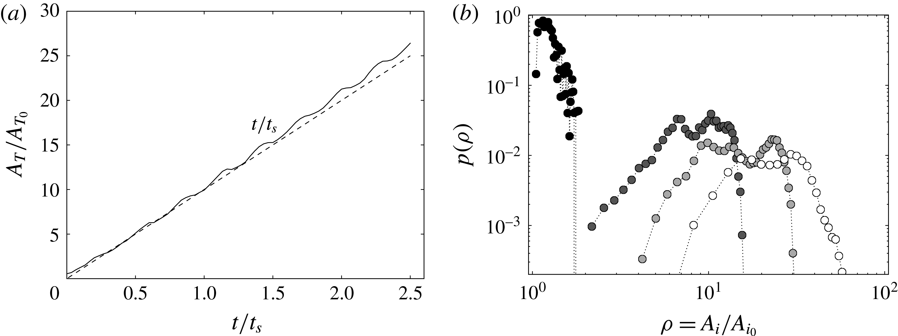
(a) The temporal evolution of the total area
 $A_{T}$
(solid line) of the full numerical sheet used to model the experiment compared with a linear growth with time (dashed line). (b) The probability density function of elongations
 $\unicode[STIX]{x1D70C}$
of the areas
 $A_{i}$
of the triangular elements for
 $t\sim 0.07\,t_{s}$
(black),
 $t=0.5\,t_{s}$
(dark grey),
 $t=0.83\,t_{s}$
(light grey) and
 $t=1.3\,t_{s}$
(white), where
 $t_{s}$
refers to the longest mixing time along the sheet.

In the experiment, the blob of dye is injected with a small but finite radial extent such that the surface of the sheet is expected to grow linearly with time. The total area
 $A_{T}$
of the sheet computed numerically is plotted in figure 14(a) as a function of time. It increases linearly despite small and evanescent periodic modulations, a linear growth of the surface elements consistent with the scaling law of the maximal concentration as
 $t^{-3/2}$
observed experimentally and numerically.
3.6 Elongations
However, if the net sheet area and the one of all of its subelements grow linearly in time, they do not do so at the same pace: at a given instant of time, some elements have been more elongated that others. The DSM is also useful in quantifying the distribution of the elongation
 $\unicode[STIX]{x1D70C}=A_{i}/A_{i0}=s_{i0}/s_{i}$
(see (2.3)) of the triangular surface elements that constitute the sheet area. Given the calculated thickness
 $\tilde{s_{i}}=s_{i}/s_{i0}$
for each triangle, the elongation
 $\unicode[STIX]{x1D70C}_{i}=A_{i}/A_{i0}=\tilde{s_{i}}^{-1}$
is obtained as well as its probability density function
 $p(\unicode[STIX]{x1D70C})$
from the ensemble of triangles on the surface, as shown in figure 14(b). This distribution is obviously a Dirac function around
 $\unicode[STIX]{x1D70C}=1$
initially. The most probable stretching increases linearly in time, like the mean stretching, and the distribution
 $p(\unicode[STIX]{x1D70C})$
progressively broadens around it. The support of the distribution remains, however, bounded around the maximum, a sign that the stretching rates experienced by different parts of the sheet are close. This is partly due to the fact that the initial blob is very small, and is thus sensitive to the motion of nearby tori only, preventing it from visiting the entire flow, but is also due to the fact that the motion within these tori is correlated in time (the flow is stationary), preventing the multiplicative succession of stretchings/foldings which is known to be a good recipe for homogeneous mixing. This relatively narrow elongation distribution is in contrast to the one found in chaotic flows (see, for example, Meunier & Villermaux (Reference Meunier and Villermaux2010) with a two-dimensional sine flow), where
 $p(\unicode[STIX]{x1D70C})$
converges towards a lognormal broad distribution.
This fact also indicates that the nature of the stirring protocol has a profound consequence on the transient stretching histories of different subparts of a stirred blob in the flow (Varosi, Antonsen & Ott Reference Varosi, Antonsen and Ott1991), and thus on the distribution of the mixing times
 $t_{s}$
along the resulting distorted sheet, and finally on the distribution of concentration
 $p(c)$
produced by the interplay between substrate stretching and molecular diffusion, the aspect we envisage now.
3.7 The probability density function of the concentration
The quantitative measurement of the fluorescein dye concentration made in the meridional section allows us to reconstruct the three-dimensional concentration of the helix of scalar by assuming that it is advected at a constant rate by the azimuthal velocity (the so-called Taylor hypothesis). This approximation is valid since the scalar does not diffuse much during the rapid passage of the helix through the meridional laser sheet. The concentration distribution can thus be calculated at each passage of the helix by summing up the concentration level given by the pixels on each image comprising the period of the blob passage.
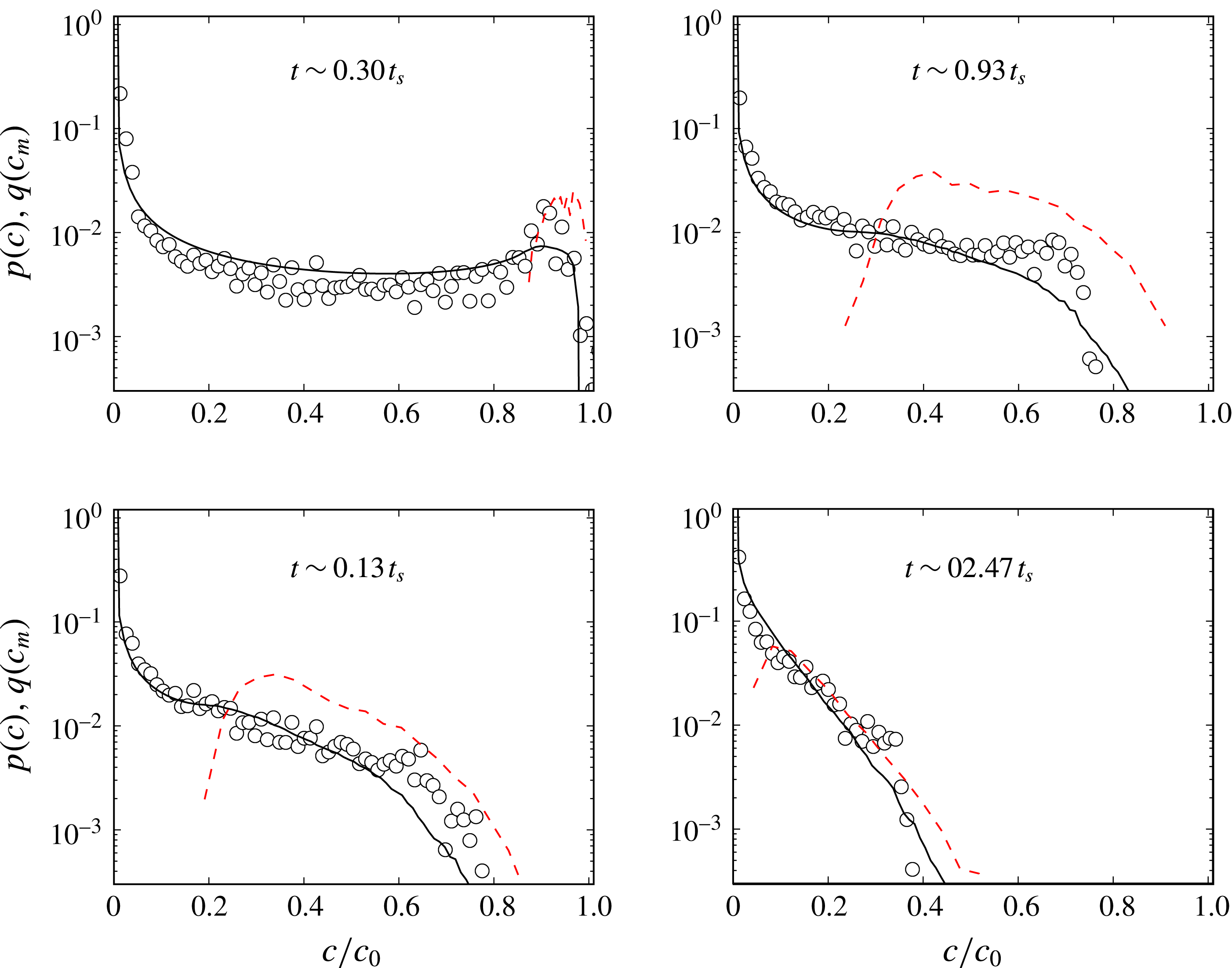
The concentration distributions
 $p(c)$
are plotted in figure 15 for four different times. At early times
 $t\sim 0.3\,t_{s}$
, that is before the mixing time, the concentration distribution has a characteristic
 $\cup$
shape (
 ${\sim}(c\sqrt{\ln [c_{M}/c]})^{-1}$
), reflecting a Gaussian-like profile of the concentration across the merely eroded sheet, with
 $c_{M}\approx 0.9\,c_{0}$
. The distribution of the maxima of concentration along the sheet
 $q(c_{m})$
, which is linked to the distribution of elongations
 $\unicode[STIX]{x1D70C}$
by
 $$\begin{eqnarray}q(c_{m})=p(\unicode[STIX]{x1D70C})\left|\frac{\text{d}\unicode[STIX]{x1D70C}}{\text{d}c_{m}}\right|,\end{eqnarray}$$
is indeed peaked around
 $c_{M}$
.
After the mixing time, diffusion tends to erode the large-concentration peak and all concentration levels are transported towards zero, the dilution concentration. As for the Batchelor vortex studied in § 2, lower concentration levels sit in the most stretched area and are thus proportionally more numerous, therefore modifying the shape of
 $p(c)$
into a globally decaying distribution in
 $c$
, the most probable levels being close to
 $c=0$
at maximal dilution, as seen in figure 15. In this way, the maximum concentration
 $c_{M}$
has dropped to a third of the initial concentration at
 $t\sim 2.47\,t_{s}$
.
Comparison of the scalar concentration levels obtained experimentally (circles) and numerically (solid lines) at
 $Re=120$
and
 $Pe=6\times 10^{6}$
at progressive stages referred to the mixing time
 $t_{s}=35$
s. The maximal concentration distributions
 $q(c_{m})$
are plotted as red dashed lines.

The distribution
 $p(c)$
is reconstructed by the DSM as explained in § 2, assigning to each triangular element constituting the sheet a Gaussian spatial profile of width
 $s_{i}\sqrt{\unicode[STIX]{x1D70F}_{i}}$
(see (2.18) and (2.24)). This straightforward calculation in the DSM scheme provides a correct prediction of the real concentration distribution as long as the sheet does not reconnect with itself. This is the ‘solitary strip’ or ‘solitary sheet’ limit described by Meunier & Villermaux (Reference Meunier and Villermaux2010) and more recently by Le Borgne et al. (Reference Le Borgne, Dentz and Villermaux2015), which suits the high-Péclet-number and/or intermediate-time limit. The strongly diffusive limit, at large times, involves necessarily, by contrast, diffusive overlaps between subparts of the sheet. In this case, the scalar field reconstruction described in § 2.4 is mandatory to obtain the full concentration field. The solitary sheet assumption is nevertheless correct here within the times displayed in figure 15 (see, however, figure 16), the DSM calculation, without field reconstruction, succeeding in representing the measured concentration distribution well.
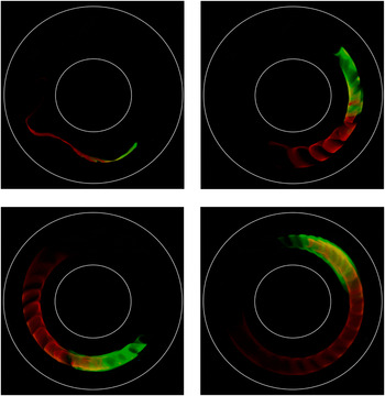
Top-view picture of an elongated blob of fluorescein (leading green half) and rhodamine (following red half) in the Taylor–Couette set-up turning counterclockwise in progressive pictures globally illuminated with an LED white-light array. The injection was performed with a single pipette half filled with rhodamine (red) and the other half with fluorescein (green).

It should be noted finally that
 $p(c)$
is progressively well approximated by
 $q(c_{m})$
, a fact originally discussed by Meunier & Villermaux (Reference Meunier and Villermaux2003), who explained how the variability in
 $c_{m}$
caused by the distribution of elongations overcomes in
 $p(c)$
that due to the Gaussian transverse profile at large times. This fact has, since then, allowed a transparent discussion on the status of
 $p(c)$
in the fully overlapping aggregation regime (Villermaux & Duplat Reference Villermaux and Duplat2003; Duplat & Villermaux Reference Duplat and Villermaux2008; Meunier & Villermaux Reference Meunier and Villermaux2010; Le Borgne et al.
Reference Le Borgne, Dentz and Villermaux2015).
4 Conclusions
The purpose of this work was to extend the diffusive strip method (DSM) originally proposed by Meunier & Villermaux (Reference Meunier and Villermaux2010) to its ‘sheet’ version suitable for modelling scalar mixing in three dimensions. The numerical adaptation of this method was achieved by employing a triangulation method (Popinet Reference Popinet2010) to parametrize the surface of a blob, soon deformed as a sheet by three-dimensional stirring fields. Across each triangle, a transverse diffusive problem is solved in suitably modified space–time coordinates, as a function of the local deformation rate. The method is, like its two-dimensional version, close to exact in the sense that the only components of the concentration gradients that are not represented are those that are rendered negligible by the dynamics, that is, those along the sheet.
The method was first validated against an accurate DNS in a modified Batchelor vortex at moderate Péclet number (§ 2) and then confronted with detailed experimental measurements in a Taylor–Couette cell, at much higher Péclet number (§ 3). In both cases, a blob initially injected into the stirring field shapes into a helical sheet, whose local concentration decays in time
 $t$
as a result of a coupling between elongation and molecular diffusion, like
 $t^{-3/2}$
, earlier when the sheet element has been more stretched. A distribution of concentration arises from the variability of the sheet element elongation at a given instant of time, very well represented by the DSM, whether at moderate Péclet number on a model flow when the DNS can be a judge of it or at large Péclet number when experiments in the real world are the natural reference.
The method amounts to computing the deformation of a scalar sheet in a flow, following its local stretching rate and thickness, and we have shown that this information is sufficient to reconstruct the three-dimensional concentration field around it a posteriori, including diffusive effects. The power of this method lies in its proximity to first principles (it is a reformulation of the diffusion equation on a moving substrate) and its simplicity: the computation is to be made only once and the concentration field is obtained for any value of the scalar diffusivity or initial sheet size from a unique simulation with no additional numerical cost (figure 2).
This method is particularly well suited to representing transient mixing, in any stirring protocol, irrespective of the mean stretching law, be it algebraic, as in the cases investigated here (where material lines grow proportionally to time), exponential (like in chaotic flows producing Baker transforms) or even super-exponential flows (occurring as transients in developing instabilities; see, e.g., de Rivas & Villermaux Reference de Rivas and Villermaux2016). The reason is that the kinematics of the flow is all absorbed in the Ranz transformation (see (2.6)) mapping any particular case to a diffusion equation. In this respect, the method will equally apply to chaotic flows with steady or time-dependent protocols (Cartwright, Feingold & Piro Reference Cartwright, Feingold and Piro1996) and turbulent flows.
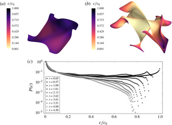
Mixing of a blob in an ABC flow with
 $A=B=C=1$
,
 $Pe=7500$
and
 $Pe_{0}=12$
with
 $s_{0}=0.1$
for (a)
 $t=0.95\,t_{s}$
and (b)
 $t=4.5\,t_{s}$
. (c) Concentration distributions
 $P(c)$
for increasing times normalized by the mixing time
 $t_{s}$
.

As it is now, the drawback of the method is that as a blob is progressively deformed and expanded in a flow, it has to be more refined to be accurately represented. For instance, in the deformation fields considered here, the sheet area grows linearly in time, and thus so does the number of triangles needed to cover it. This inflation has a numerical cost. However, a not-yet-implemented mesh-coarsening process has been studied to delete triangles reaching concentration values below a given threshold in order to preserve the high efficiency of the method when applied to complicated flows. There is indeed no need to over-resolve sheet subareas that are basically flat (a few large triangles are sufficient for these regions which are the rule rather than the exception, see, e.g., figure 10) or those bearing a very small concentration, close to the trivial dilution level (which carry no useful information). This easily implemented modification of the method will naturally limit the inflation. It might prove very useful for long runs in chaotic flows with mean exponential area stretching. However, the application of the method at its present stage of development to an Arnold–Beltrami–Childress (ABC) flow (Dombre et al.
Reference Dombre, Frisch, Greene, Hénon, Mehr and Soward1986) poses no difficulty at least when the simulation runs for up to a few average mixing times. As seen in figure 17, the concentration levels are close to bimodally distributed when
 $t/t_{s}\ll 1$
, and there is no trace of the initial concentration
 $c=c_{0}$
anymore at
 $t=4.5\,t_{s}$
, showing that the medium is then appreciably mixed, as expected. Similarly to the linear flows studied here, the concentration distribution
 $P(c)$
is uniformly decreasing in the ABC flow, reflecting the fact that lower concentration levels
 $c$
lie on more stretched, and thus proportionally more numerous, portions of the deformed blob.
Another more subtle issue concerns the possible interaction of the sheet with itself, the phenomenon we have called diffusive overlap, or aggregation, which is known to be at the root of the build-up of non-academic stirred concentration fields. This ingredient was not considered here, although it concerns the very late stages of the helical sheet dilution, as illustrated in figure 16. The injected blob was on purpose composed of two colour dyes (fluorescein and rhodamine), and it is seen that, when the sheet diffuse boundaries have grown enough, overlap stars to occur. At these very late stages, the helix parts are intertwined and start to interact, invading regions that share the contributions of both dyes. In that limit, the overall concentration field must be reconstructed according to the method described in § 2.4. However, triangle merging or deletion in the overlapping regime remains a challenging issue for the DSM.
Acknowledgements
The Agence Nationale de la Recherche (ANR) is acknowledged for funding of the ANR-DFG grant TurbMix (ANR-14-CE35-0031-01). We thank S. Popinet for useful discussions and advice on the GTS library details and its potential applications. This library is available at http://gts.sourceforge.net/. Computational results are visualized employing a Python-based tool for 3D plotting, Mayavi: 3D scientific data visualization and plotting in Python (Ramachandran & Varoquaux Reference Ramachandran and Varoquaux2011).