
1. Introduction
Turbulent bubbly flow is encountered in many practical applications. Examples are heat exchangers in power plants, or cooling systems of nuclear reactors. The simultaneous existence of physical phenomena spanning a wide range of scales of motion is certainly one, if not the most, complex aspect of bubbly multiphase flows. Experimental studies of bubble-laden flows are particularly challenging. Non-intrusive imaging techniques (Lau, Deen & Kuipers Reference Lau, Deen and Kuipers2013) are, in fact, currently limited to very dilute void fractions (Mercado et al. Reference Mercado, Gomez, Van Gils, Sun and Lohse2010). In this scenario, despite other limitations, direct numerical simulation (DNS), where all the relevant scales of motion are resolved by the computational grid and time step, proves to be a tool of paramount importance for a deeper understanding of the physics of bubbly flows. In particular, wall-bounded turbulence and its interaction with bubbles can be analysed by simulating a turbulent channel flow (Kim, Moin & Moser Reference Kim, Moin and Moser1987; Moser, Kim & Mansour Reference Moser, Kim and Mansour1999; Vreman & Kuerten Reference Vreman and Kuerten2014). The latter constitutes a fundamental configuration where all the relevant features of the physics of the problem can be analysed. The doubly periodic domain and the simple geometry allow us to reduce three-dimensional quantities to averaged one-dimensional profiles for which a clear interpretation can be drawn.
A comprehensive review of DNS of bubbly flows is presented in Tryggvason et al. (Reference Tryggvason, Dabiri, Aboulhasanzadeh and Lu2013). Bubble-laden channel flows are scarcely investigated compared to turbulent single-phase channel flows. This is primarily due to the extreme computational resources needed to carry out such simulations where bubble motion and deformability have to be resolved. In the pioneering work by Lu & Tryggvason (Reference Lu and Tryggvason2006) a relatively small channel (referred to as ‘minimum channel’) at  $Re_\tau =127$ was simulated for different gas volume fractions. This study focused on volume fraction and velocity statistics in a downflow channel as a function of the gas concentration. For nearly spherical bubbles migration towards the core of the channel was observed at statistically steady state. A significant reduction of the mass flow rate was observed when imposing the shear stress at the walls. Furthermore, the wakes generated by the rising motion of the bubbles were found to strongly increase the velocity fluctuations in the core region. In contrast, a reduction of the turbulence intensities close to the wall was reported. In subsequent studies, the effect of bubble size (Lu & Tryggvason Reference Lu and Tryggvason2007) and bubble deformability (Lu & Tryggvason Reference Lu and Tryggvason2008) were investigated. A reduction in the lateral lift for highly deformed bubbles was observed in an upflow configuration. The latter findings on upflow configurations were furthermore confirmed in a later study of the same authors carried out at
 $Re_\tau =250$ (Lu & Tryggvason Reference Lu and Tryggvason2013). It is worth mentioning the work of Santarelli & Fröhlich (Reference Santarelli and Fröhlich2015, Reference Santarelli and Fröhlich2016) where a relatively large number of bubbles, approximated as rigid spheres, was simulated in an upflow channel. Moreover, a constant density and viscosity field in the governing equations was used. Despite the simplifying assumptions, these studies revealed useful insights into turbophoresis effects and bubble clustering.
To improve the understanding of the complex flow structure in bubble-laden channel flows, this paper focuses on a local flow topology analysis based on the invariants of the velocity-gradient tensor following the pioneering work of Chong, Perry & Cantwell (Reference Chong, Perry and Cantwell1990) and Perry & Chong (Reference Perry and Chong1987). In the case of incompressible flows, all possible small-scale flow structures can be categorized into two nodal and two focal topologies. Regarding the general distribution of flow topologies in single-phase channel flows, important observations have already been made by Blackburn, Mansour & Cantwell (Reference Blackburn, Mansour and Cantwell1996): ‘Probability density functions of tensor invariants for the outer regions of the channel flow showed a similarity to other turbulent flows with apparent preference for stable focus/stretching and unstable node/saddle/saddle topologies’. Using DNS data of wall-bounded shear flows with zero-pressure-gradient as well as boundary layers with separation and reattachment, Chong et al. (Reference Chong, Soria, Perry, Chacin, Cantwell and Na1998) examined turbulence structures from the viewpoint of the attached eddy hypothesis. The generation of Reynolds stress, turbulent kinetic energy and dissipation in a low Reynolds number turbulent boundary layer have been studied by Chacin & Cantwell (Reference Chacin and Cantwell2000). It has been found that the strongest Reynolds stress and turbulent kinetic energy generating events occur where the discriminant of the velocity-gradient tensor has a rapid change of sign. Chacin & Cantwell (Reference Chacin and Cantwell2000) further demonstrated how the time evolution of the invariants can be studied by computing along particle paths in a Lagrangian frame of reference. Apparently, the invariants tend to evolve towards two distinct asymptotes in the plane of invariants. Several simplified models for the evolution of the velocity-gradient tensor are additionally described.
In the context of incompressible two-phase flows, Hasslberger, Klein & Chakraborty (Reference Hasslberger, Klein and Chakraborty2018) analysed the distribution of local flow topologies in bubbly air–water systems. It has been found that focal topologies, representing vortical motion, predominantly reside inside the gaseous bubbles. However, the work of Hasslberger et al. (Reference Hasslberger, Klein and Chakraborty2018) was limited to two interacting bubbles at a technically relevant bubble Reynolds number – in contrast to the present study where (dense) bubble swarms are examined. The behaviour of flow topologies in the primary atomization of liquid jets has been investigated by Hasslberger et al. (Reference Hasslberger, Ketterl, Klein and Chakraborty2019a) who introduced a simple model for the size distribution of coherent structures. The latter model's validity is also tested in the context of this work. Recently, Dodd & Jofre (Reference Dodd and Jofre2019) reported on small-scale flow topologies in decaying isotropic turbulence laden with finite-size droplets. Focusing on the carrier phase close to the interface, the invariants calculation has been conditioned on the distance from the droplet surface. It has been shown that, outside the viscous region near the interface, the flow topology distribution is in agreement with homogeneous isotropic turbulence. Inside the viscous layer at the droplet surface, the flow topologies shift from a preference for high-enstrophy/low-dissipation motions to a preference for low-enstrophy/high-dissipation. According to Dodd & Jofre (Reference Dodd and Jofre2019), the shapes of the invariant distributions at the droplet surface are very similar to those reported in the literature for the viscous sublayer of turbulent wall-bounded flows. Similarly, a particular focus is placed on the vicinity of the interface in the present study. The behaviour on both sides of the interface is important in finding a universal modelling strategy for under-resolved two-phase flow simulations. Due to the vorticity accumulation effect in the lighter phase of turbulent two-phase flows (Dixit & Govindarajan Reference Dixit and Govindarajan2010; Tripathi, Sahu & Govindarajan Reference Tripathi, Sahu and Govindarajan2014), conclusions on the flow structure close to the interface may well be different for bubble- and droplet-laden flows.
Insightful applications of flow topology analysis are also available in the context of (compressible) reactive flows (Wacks et al. Reference Wacks, Chakraborty, Klein, Arias and Im2016; Chakraborty et al. Reference Chakraborty, Wacks, Ketterl, Klein and Im2019; Han et al. Reference Han, Scholtissek, Dietzsch, Jahanbakhshi and Hasse2019), but shall only be mentioned for completeness due to the largely different physics involved. Further academic configurations, like isotropic turbulence, are studied by Ooi et al. (Reference Ooi, Martin, Soria and Chong1999) and Elsinga & Marusic (Reference Elsinga and Marusic2010), for instance.
The foremost goal of this study is to improve the fundamental understanding of coherent structures in bubble-laden channel flows. The analysis of flow topologies and coherent structures is key to the understanding of undoubtedly complex turbulent flows because they allow for a characterization of the flow by means of mathematically well-defined canonical flow types. Adding the multiphase character to turbulent flows makes the situation even more complicated. Hence, to draw a clear picture of the multi-physics problem, statistics like the probability of different flow types are evaluated in a phase-conditional manner – without the different flow behaviours in both phases masking each other. Using this mathematical tool, a direct comparison between flow structures induced by the channel walls and by the dense swarm of (interacting) bubbles is facilitated. Furthermore, the differences and similarities between laminar and turbulent bubble-laden flows are highlighted and the wall-interface analogy is discussed.
The observations and conclusions from this study might also inspire the identification of universal features of the flow which can later be exploited for a simplified description, i.e. modelling, of these flows. One possibility for sub-grid modelling is the well-established eddy viscosity concept. In a recent contribution by Fang, Wang & Bergstrom (Reference Fang, Wang and Bergstrom2019), (classical) vortex identifiers, e.g. the famous  $\lambda _2$- and
 $Q$-criteria (defined in § 2), are used to build eddy viscosity sub-grid-scale models for large eddy simulation. The building of eddy viscosity sub-grid-scale models using invariants is also extensively discussed by Trias et al. (Reference Trias, Folch, Gorobets and Oliva2015). Another example is the model of Kobayashi (Reference Kobayashi2005), which uses the coherent structure function. Since all of these models are based on the second (and third) invariant of the velocity-gradient tensor, the connection to the flow type classification in this paper becomes clear, cf. § 2 on the mathematical background. However, to develop and test such models is beyond the scope of this work. In terms of more advanced than eddy viscosity modelling, in particular accounting for the two-phase nature of the flow, it is an important first step to understand deviations from the well-known single-phase flow behaviour. Thus, the present analysis focuses on the physics of flow topology distributions conditional on different phases.
The underlying DNS database stands out for the high bubble count, the wide range of gas concentrations, the large channel flow domain and the fact that no simplifying assumptions on the bubble motion and deformation were used. Different techniques for accurate interface propagation have been developed over the years, most prominently the front-tracking method, the level-set method, the volume-of-fluid (VOF) method and combinations thereof – featuring specific advantages and disadvantages each. The VOF method has been chosen for this study due to its inherent volume conservation property and ability to deal with strong interface deformations as well as topological changes (although breakup does not occur for the bubble regime considered here). The issue of spurious numerical bubble coalescence has been avoided by a novel multi-marker geometrical VOF method (Cifani Reference Cifani2017; Cifani, Kuerten & Geurts Reference Cifani, Kuerten and Geurts2018).
2. Mathematical background
The invariants of the velocity-gradient tensor
 \begin{equation} A_{ij} \equiv \frac{\partial u_i }{\partial x_j}=S_{ij}+W_{ij} \end{equation}
give rise to a set of canonical flow types, i.e. local flow topologies (Perry & Chong Reference Perry and Chong1987; Chong et al. Reference Chong, Perry and Cantwell1990). This tensor's symmetric and anti-symmetric components are represented by  $S_{ij}=0.5(A_{ij}+A_{ji})$ and
 $W_{ij}=0.5(A_{ij}-A_{ji})$, respectively. The corresponding characteristic equation
 $\lambda ^3+P\lambda ^2+Q\lambda +R=0$ exhibits three solutions, i.e. the eigenvalues
 $\lambda _1$,
 $\lambda _2$ and
 $\lambda _3$ of
 $A_{ij}$. Since the first invariant of
 $A_{ij}$ reads
 \begin{equation} P \equiv -\mathrm{trace}(A_{ij})=-(\lambda_1+\lambda_2+\lambda_3) = - S_{ii}= 0 \end{equation}
for incompressible flows ( $\partial u_i / \partial x_i=0$), the second and third invariants of
 $A_{ij}$ reduce to
 \begin{equation} Q \equiv (\mathrm{trace}(A_{ij})^2-\mathrm{trace}(A_{ij}^2))/2=(-S_{ij}S_{ij}+W_{ij}W_{ij})/2 \end{equation}
and
 \begin{equation} R \equiv -\det(A_{ij})=(-S_{ij}S_{jk}S_{ki}-3W_{ij}W_{jk}S_{ki})/3 \end{equation}
for the case considered here. The characteristic equation's discriminant
 \begin{equation} D=(27R^2+4Q^3)/108 \end{equation}
divides the  $Q{-}R$ phase space into two regions:
 $D>0$ where
 $A_{ij}$ shows one real eigenvalue and two complex conjugate eigenvalues (hence focal topologies), and
 $D<0$ where
 $A_{ij}$ shows three real eigenvalues (hence nodal topologies). Corresponding to
 $D=0$, two lines separating the topologies in the phase space are specified by
 \begin{gather} r_{1a}=-2(-3Q)^{3/2}/27, \end{gather}
 \begin{gather}r_{1b}=+2(-3Q)^{3/2}/27. \end{gather}
In the region  $D>0$,
 $A_{ij}$ exhibits purely imaginary eigenvalues on the line
 \begin{equation} r_2=0. \end{equation}
The lines  $r_{1a}$,
 $r_{1b}$ and
 $r_2$ divide the
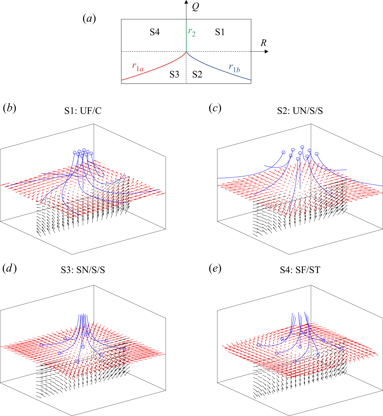
 $Q{-}R$ phase space into four canonical flow topologies in the incompressible case. In addition to the topology borders
 $r_{1a}$,
 $r_{1b}$ and
 $r_2$ in the
 $Q{-}R$ phase space, a graphical representation of flow topologies S1 to S4 is shown in figure 1. It is further instructive to split the second invariant
 $Q$ into two parts,
 \begin{equation} Q = Q_S + Q_W = {- S_{ij}S_{ij}/2} + {W_{ij} W_{ij}/2}, \end{equation}
where  $Q_S$ and
 $Q_W$ denote the second invariants of
 $S_{ij}$ and
 $W_{ij}$, respectively;
 $Q_S$ remains a negative quantity since
 $-4\nu Q_S=2\nu S_{ij}S_{ij}$, i.e. the dissipation of kinetic energy into heat per unit mass, where
 $\nu$ is the kinematic viscosity. The latter part,
 $Q_W$, is directly related to vorticity
 $\omega _i$ and enstrophy
 $\omega _i \omega _i /2$ according to
 $W_{ij} W_{ij}/2 = \omega _{i} \omega _{i} / 4$. Thus,
 $Q<0$ is indicative of strain-dominated regions and
 $Q>0$ is indicative of vorticity-dominated regions. In a similar manner, the generation (or destruction) of dissipation and enstrophy is reflected in the corresponding parts of the third invariant
 $R$.
Classification of flow topologies S1 to S4 and projection of topology borders  $r_{1a}$,
 $r_{1b}$ and
 $r_2$ in the
 $Q$–
 $R$ plane for the incompressible case
 $P=0$ (a). Dashed lines indicate
 $Q=0$ and
 $R=0$, respectively; graphical representation (b–e) corresponding to UF = unstable focus,
 $\text {UN} = \text {unstable node}$,
 $\text {SN} = \text {stable node}$,
 $\text {SF} = \text {stable focus}$,
 $\text {C} = \text {compressing}$,
 $\text {S} = \text {saddle}$,
 $\text {ST} = \text {stretching}$. The blue circles indicate the origin of the blue streamlines.

3. Numerical method and computational set-up
The incompressible Navier–Stokes equations have been solved numerically by employing the massively parallel code detailed in Cifani (Reference Cifani2017) and Cifani et al. (Reference Cifani, Kuerten and Geurts2018). The latter has been designed to efficiently handle up to  $O(10^4)$ fully deformable bubbles in wall-bounded turbulence. By means of a modified pressure-correction formulation, the use of a fast-Poisson solver is made possible while retaining an accurate numerical solution at high density ratios (Cifani Reference Cifani2019). In the framework of the finite-volume method, spatial discretization on a staggered grid is implemented by the third-order quadratic upstream interpolation for convective kinematics (QUICK) scheme for momentum advection and the second-order central differencing scheme for diffusive fluxes. A second-order Adams–Bashforth scheme is used for the time marching. The volume fraction field is advected by means of a geometrical VOF method based on piecewise-linear interface calculation. Hence, in the three-dimensional simulations, a planar phase interface is reconstructed in all computational cells occupied by volume fractions between 0 and 1. This guarantees sharpness of the volume fraction field and a mass loss within a fraction of a percentage (Cifani et al. Reference Cifani, Michalek, Priems, Kuerten, van der Geld and Geurts2016). The multi-marker formulation applied here (Cifani Reference Cifani2017; Cifani et al. Reference Cifani, Kuerten and Geurts2018) assigns a separate volume fraction field (of limited size, only in the vicinity of the considered bubble) to each bubble to avoid spurious numerical bubble coalescence which would frequently occur for the single-marker formulation. For the bubble size and fluid properties investigated in this work, characterized by the Weber/Eötvös number, physical bubble coalescence is assumed to be very unlikely. Instead, we focus on the dynamics generated by a given number of bubbles whose interaction result in bouncing. The same set-up was, for example, adopted by Lu & Tryggvason (Reference Lu and Tryggvason2006). Physical coalescence can in principle be introduced by assigning a single marker function to two colliding bubbles. An example of such strategy has been proposed in Kwakkel, Breugem & Boersma (Reference Kwakkel, Breugem and Boersma2013) where a film drainage model has been developed to determine the occurrence of physical coalescence. While the extension to physical coalescence goes beyond this study, it could represent an interesting development for future investigations. Surface tension is accurately accounted for by using the generalized height function method (Popinet Reference Popinet2009; Cifani et al. Reference Cifani, Kuerten and Geurts2018).
The rectangular domain of size  $4{\rm \pi} H \times 2 H \times 4{\rm \pi} H/3$, where
 $H$ is the channel half-width, is uniformly discretized by
 $1152 \times 240 \times 384 \approx 1.06 \times 10^8$ cells. Thus, the computational grid is slightly finer in the wall-normal direction owing to the wall influence. Accurately capturing the dynamics of nearly spherical bubbles requires more than 15 cells per diameter in the framework of the geometrical VOF method according to Cifani et al. (Reference Cifani, Kuerten and Geurts2018). Regarding the resolution of the flow, Uhlmann (Reference Uhlmann2008) shows that 15 cells per diameter is sufficiently fine for a bubble Reynolds number of 130 which is close to the values investigated here. Since more than 20 cells per spherical diameter are used in this work, the mesh resolution is considered to be high enough. No-slip wall boundary conditions are imposed in the
 $y$-direction, whereas periodic boundary conditions are imposed in the mean flow direction
 $x$ and the homogeneous direction
 $z$. The density and dynamic viscosity ratio of both phases are specified as
 $\rho _l / \rho _g = 20$ and
 $\mu _l / \mu _g = 20$ as a default. Additionally, a comparison between
 $\mu _l / \mu _g = 20$ and
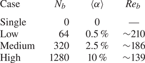
 $\mu _l / \mu _g = 1$ is presented in § 4.6. An overview of the simulation parameters in terms of the bubble count
 $N_b$, overall void fraction
 $\langle \alpha \rangle$ and bubble Reynolds number
 $Re_b$
 \begin{equation} Re_b = \frac{u_{x,rel} d_b }{\nu_l} \end{equation}
is given in table 1. The relative axial velocity of both phases is calculated as  $u_{x,rel}=\langle u_x \rangle _l - \langle u_x \rangle _g$, where the phase-conditional spatial averaging
 $\langle \cdot \rangle _{l,g}$ is limited to the bulk part of the domain (
 $0.5<y/H<1.5$), excluding the wall boundary layers. In all cases, the bubble diameter
 $d_b$, the gravity in the mean flow direction
 $g$ and the surface tension coefficient
 $\sigma$ are chosen such that an Eötvös number of
 $Eo=(\rho _l-\rho _g)gd_b^2/\sigma =0.633$ is obtained. Since the simulation is based on a fixed mass flow rate resulting in a constant bulk Reynolds number of
 \begin{equation} Re = \frac{\langle u_x \rangle_l H }{\nu_l} \approx 3.1 \times 10^3, \end{equation}
the friction Reynolds number
 \begin{equation} Re_\tau = \frac{u_\tau H }{\nu_l} = \frac{\sqrt{\tau_w /\rho_l} H }{\nu_l} \approx 180 \end{equation}
based on the wall shear stress  $\tau _w$ is slightly modified by the inclusion of bubbles.
DNS case overview in terms of bubble count  $N_b$, void fraction
 $\langle \alpha \rangle$ and bubble Reynolds number
 $Re_b$.

4. Results and discussion
4.1. Analytical reference solution
As the subsequent discussion on the numerical results reveals, several features of the complex bubble-laden channel flow can be explained by utilizing an analogy to much simpler generic laminar flows. For this reason, an analytical flow topology analysis (as introduced in § 2) on laminar bubble-affected flows in the creeping flow regime (Hasslberger, Marten & Klein Reference Hasslberger, Marten and Klein2019b) is briefly reviewed here. The underlying field descriptions are based on the analytical solutions of Hadamard & Rybczynski (see Sadhal, Ayyaswamy & Chung Reference Sadhal, Ayyaswamy and Chung2012) for far-field boundary conditions (i.e. undisturbed parallel flow imposed at infinite distance  $r \rightarrow \infty$ from the bubble centre) and Satapathy & Smith (Reference Satapathy and Smith1961) for near-field boundary conditions (i.e. undisturbed parallel flow imposed at a finite distance from the bubble centre). In the example presented, the near-field boundary conditions are imposed at
 $r/r_b=3$. The dynamic viscosity ratio
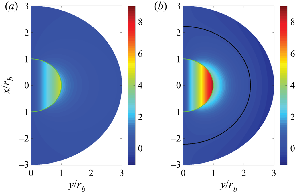
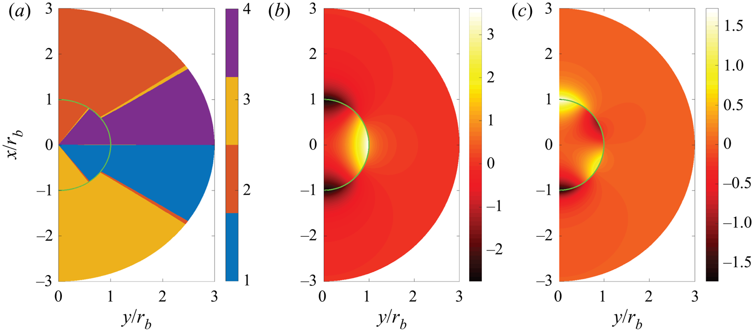
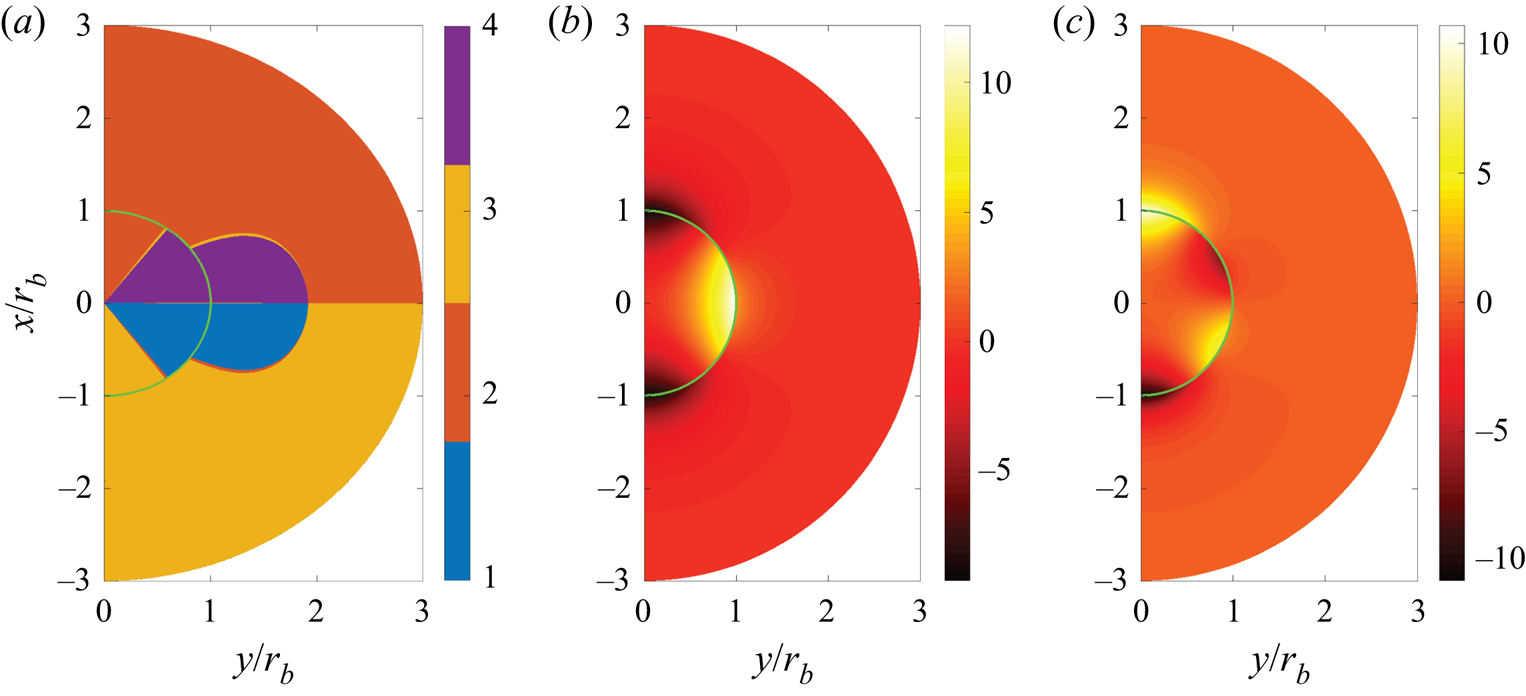
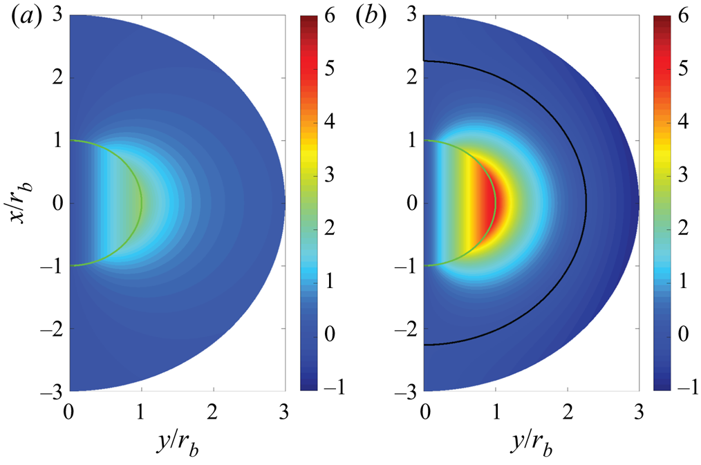
 $\mu _l / \mu _g = 20$ is identical to the DNS database investigated below. Figure 2 shows a comparison of vorticity for both boundary condition cases. The often referenced classical solution is based on far-field boundary conditions whereas the near-field boundary conditions seem to resemble better the situation in bubble-laden channel flows including lateral confinement due to walls or bubble–bubble interactions. Due to considerable differences, especially in terms of the topology classification, both cases are discussed in this work. The corresponding fields of the second invariant
 $Q$, third invariant
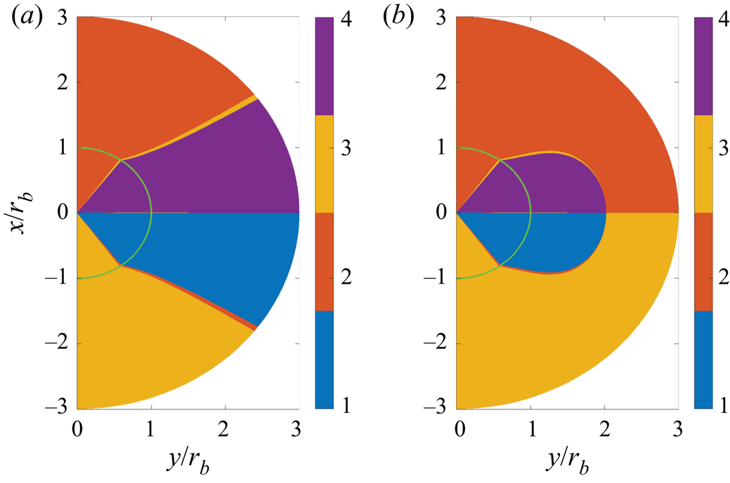
 $R$ and flow topology classification are included in figure 3 for far-field boundary conditions and figure 4 for near-field boundary conditions. In the vicinity of the bubble, a nodal-to-focal-to-nodal transition has been observed in both phases and the focal topologies (S1 and S4) are predominant in the interior phase. It has also been found that the topology distribution in the interior phase is independent of the dynamic viscosity ratio and the boundary conditions, which is not the case in the exterior phase. The focal region in the exterior phase extends to infinity for far-field boundary conditions, whereas it is bounded to a tire-like zone attached to the bubble for near-field boundary conditions. It is worth mentioning that the constant topology volume fractions in the interior phase can be derived analytically to be 10 % for nodal topologies S2/S3, and 40 % for focal topologies S1/S4 for this laminar solution. A complete mathematical description of both cases can be found elsewhere (Hasslberger et al. Reference Hasslberger, Marten and Klein2019b).
Axisymmetric analytical solution: plane-normal vorticity component  $\omega _z (d_b/u_{x,rel})$ for
 $\mu _l / \mu _g = 20$ with far-field (a) and near-field (b) boundary conditions. The main flow direction is vertical. The green and black lines indicate the interface and the zero-vorticity iso-contour, respectively.

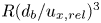
Axisymmetric analytical solution: flow topologies (a), second invariant 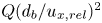 $Q (d_b/u_{x,rel} )^2$ (b) and third invariant
 $R (d_b/u_{x,rel} )^3$ (c) for
 $\mu _l / \mu _g = 20$ with far-field boundary conditions. The main flow direction is from top to bottom and the green line indicates the interface.

Axisymmetric analytical solution: flow topologies (a), second invariant 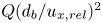 $Q (d_b/u_{x,rel} )^2$ (b) and third invariant
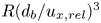 $R (d_b/u_{x,rel} )^3$ (c) for
 $\mu _l / \mu _g = 20$ with near-field boundary conditions. The main flow direction is from top to bottom and the green line indicates the interface.

4.2. Vorticity and topology fields
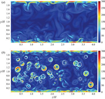
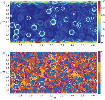
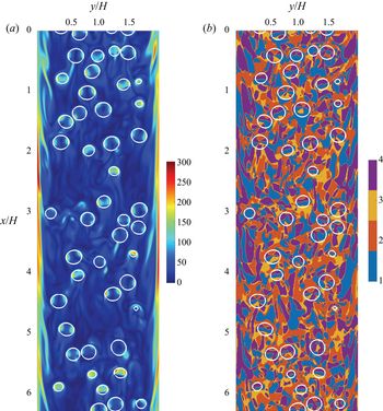
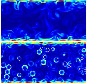
Being closely related to the analysis of flow topologies or coherent structures, the (easier-to-interpret) vorticity fields are presented in figure 5 to obtain a first qualitative impression of the simulation results. As can be expected for wall-bounded turbulent flows, vorticity levels in the wall boundary layer are high for both extreme cases discussed here, the single-phase flow ‘single’ as well as the two-phase flow with the highest bubble count ‘high’. In addition, elevated vorticity levels can be observed in the vicinity of the interface for two-phase flows when the bubbles are cut at their mid-plane. The comparison of figure 5(b) with the analytical creeping flow solution in figure 2 reveals an obvious similarity, namely the torus-like region (whose axis points in mean flow direction) of elevated vorticity in the vicinity of the interface.
Spanwise slices of vorticity magnitude 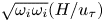 $\sqrt {\omega _i \omega _i} (H/u_\tau)$ at
 $x=L_x/2$ for case ‘single’ (a) and case ‘high’ (b). Interface coloured white.

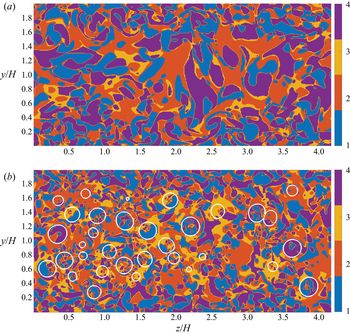
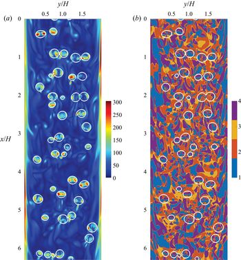
The corresponding discrete topology fields at the same location can be found in figure 6. Several interesting observations can be made which will be quantified in the following sections. The behaviour in the wall boundary region is similar for the ‘single’ and ‘high’ cases since the bubbles are rarely penetrating into that region (cf. volume fraction distribution in figure 9). However, clear differences are identified in the bulk part of the domain. The bubbles are acting as mixing elements and fragmenting the large topology structures. As the axisymmetric analytical solution already suggests, the flow behaviour in the lateral and axial directions is different. Hence, in addition to spanwise slices, axial slices of the vorticity and topology fields are depicted in figure 7. Although the situation in the DNS is not as symmetric as in the analytical solution, a close inspection reveals that S2 and S3 are the dominant topologies proximately ahead and in the wake of the bubbles, respectively. Since the behaviour in both phases is also different, subsequent statistics are evaluated in a conditional manner, i.e. separately for the gaseous and liquid phase.
Spanwise slices of topology fields at  $x=L_x/2$ for case ‘single’ (a) and case ‘high’ (b). Interface coloured white.

Axial slices of the first half of the channel showing the vorticity magnitude 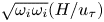 $\sqrt {\omega _i \omega _i} (H/u_\tau)$ (a) and the corresponding topology field (b) at
 $z=L_z/2$ for case ‘high’. The main flow direction is from top to bottom. Interface coloured white.

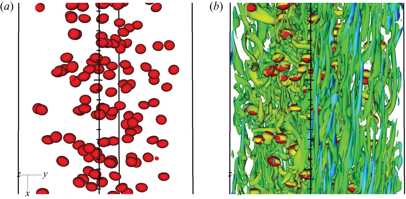
Due to the limited information from two-dimensional slices, the combination with a three-dimensional visualization in figure 8 better represents the intrinsically coherent nature of vortical structures. Consistent with earlier observations by Blackburn et al. (Reference Blackburn, Mansour and Cantwell1996), distinct vortex filaments elongated in mean flow direction are identified close to the walls. Furthermore, the bubbles mostly show a dominant tire-like focal zone (specified by  $Q (H/u_\tau )^2=100$ here) around the bubble, as predicted by the analytical reference in figure 4.
Close-up view of case ‘medium’: the red surface represents the interface and the  $Q (H/u_\tau )^2=100$ iso-contour (coloured by velocity magnitude) indicates dominant vortical structures. The main flow direction is from top to bottom.

4.3. Wall-normal and phase-conditional statistics
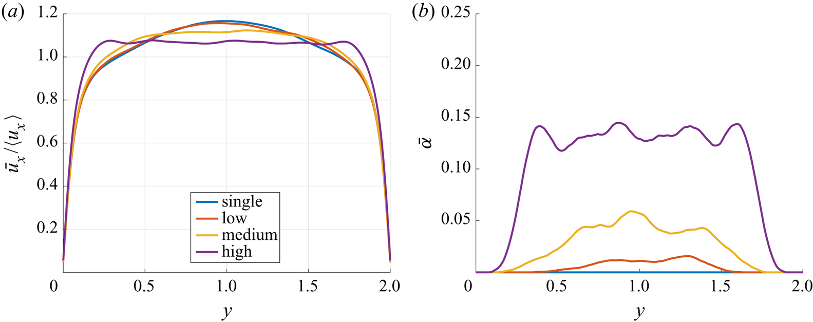
Figure 9(a) shows the wall-normal profiles of axial velocity  $\bar {u}_x$ (averaged in the
 $x$- and
 $z$-directions) for all investigated cases. Hardly any difference occurs between the single-phase flow and the two-phase flow with the lowest bubble count. In the ‘medium’ case, a flattening of the velocity profile can clearly be discerned. The highest bubble count causes further flattening of the profile and the location of maximum velocity moves from the centre of the channel towards the sidewalls, which is in agreement with earlier observations by Lu & Tryggvason (Reference Lu and Tryggvason2006). The corresponding wall-normal profiles of the gas volume fraction
 $\bar {\alpha }$ can be found in figure 9(b). In all cases, the bubbles prefer to reside in the bulk region, which is a consequence of the specific simulation set-up. As has been shown by Dabiri, Lu & Tryggvason (Reference Dabiri, Lu and Tryggvason2013), for example, the Eötvös number determines whether the bubbles are accumulating near the wall or in the bulk of the channel. Since only the fields at one time level are considered, perfectly symmetric wall-normal profiles must not be expected. Further statistics on the bubble-laden channel flow can be found in Cifani, Kuerten & Geurts (Reference Cifani, Kuerten and Geurts2020).
Normalized wall-normal profiles of slice-averaged axial velocity  $\bar {u}_x/\langle u_x \rangle$ (a) and gas volume fraction
 $\bar {\alpha }$ (b) for all cases.

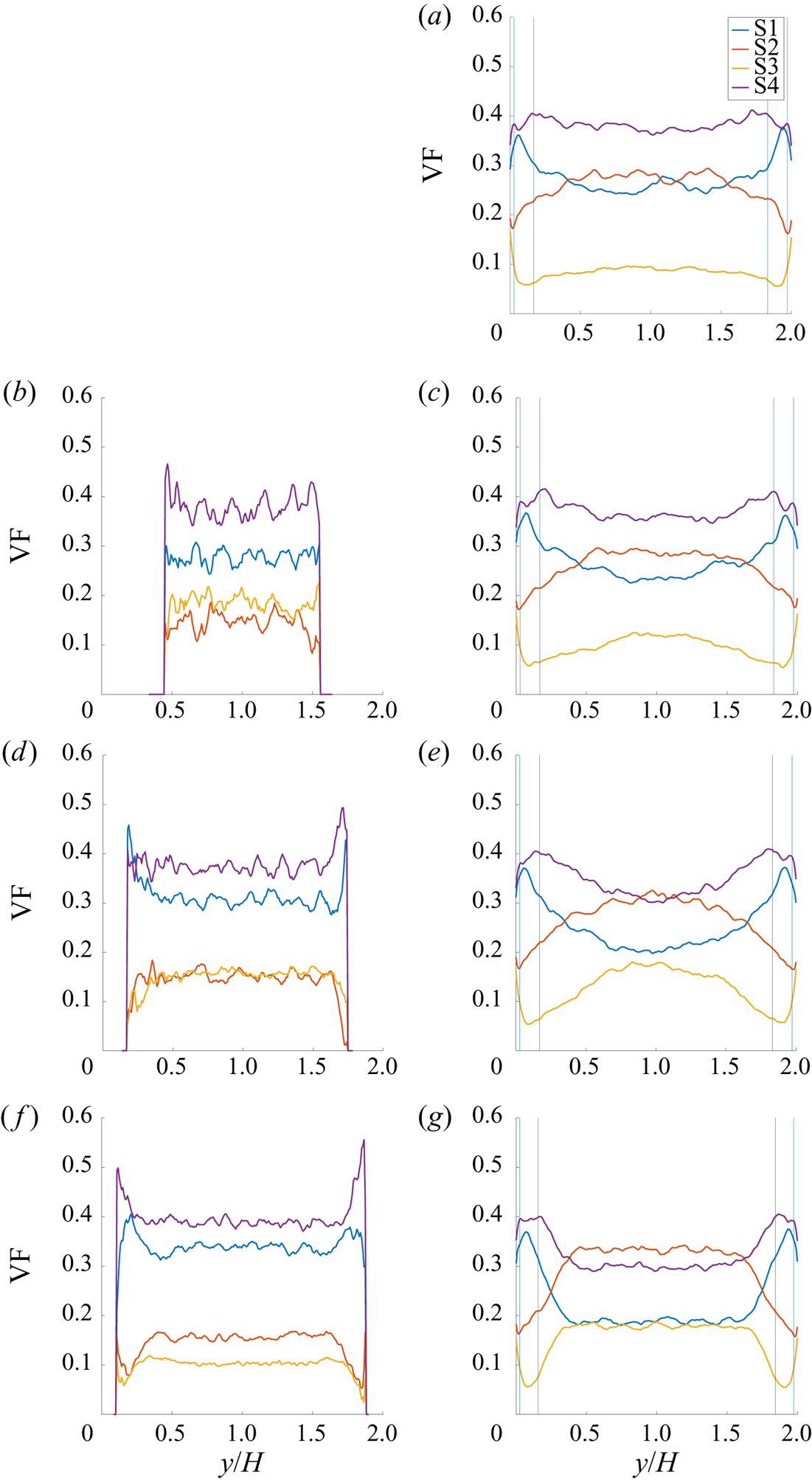
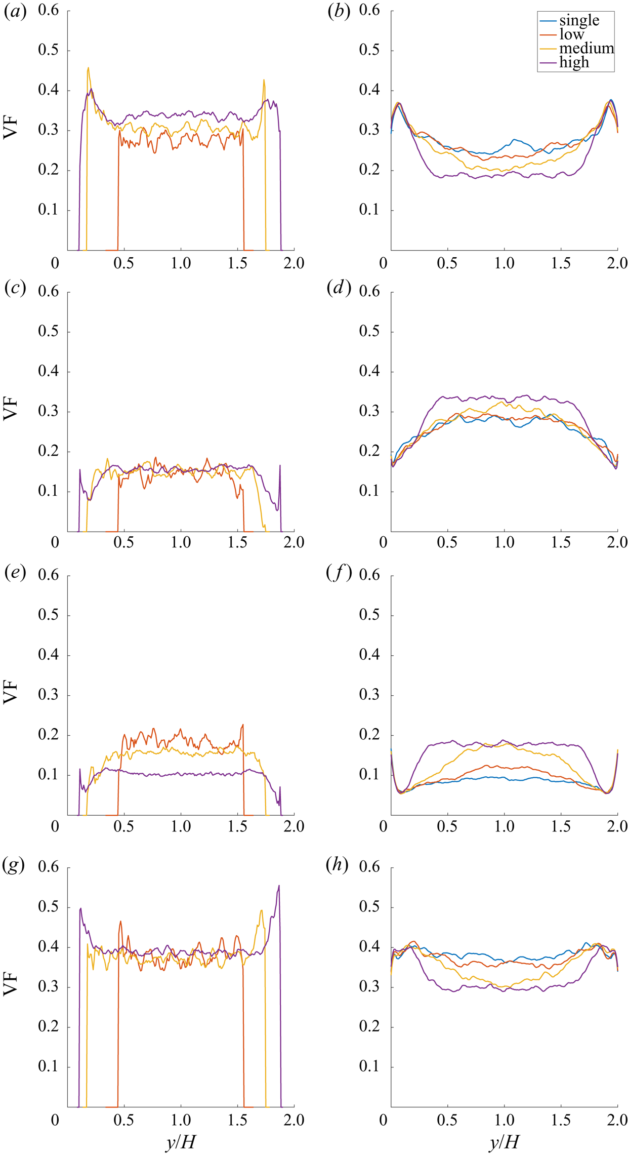
The wall-normal profiles of slice-based (i.e. with respect to horizontal planes parallel to the walls) topology volume fractions are depicted in figure 10. As one would probably expect, there seems to be a monotonic trend with increasing bubble number, i.e. from top to bottom. To highlight this aspect of the comparison in terms of topology volume fractions, figure 20 is additionally presented in the Appendix. Instead of distinguishing the different cases in the figure panels, as in figure 10, it distinguishes the different flow topologies in the figure panels. Due to the fairly monotonic trend, it is sufficient to discuss only the two extreme cases, ‘single’ and ‘high’, in the following sections. Note that the topology volume fractions depicted here are independent of the size distribution of flow structures which is discussed later in § 4.5. To distinguish wall-dominated regions from the bulk flow, estimates of the viscous–buffer layer transition ( $y+=u_\tau y/\nu _l \approx 5$) and the buffer–logarithmic layer transition (
 $y+\approx 30$) are additionally included as thin vertical lines in figure 10. The kinks in the topology volume fraction curves seem to correlate (to some degree) with the different regions of the wall boundary layer. Considering that
 $\partial u_x / \partial y$ is the only non-zero component of the velocity-gradient tensor directly at the wall, it follows that
 $Q=R=0$. Clustering at the origin is indicative of boundary layer like flow structures according to Blackburn et al. (Reference Blackburn, Mansour and Cantwell1996) but the topology classification is undefined directly at the
 $Q$-
 $R$-origin. Thus, the topology classification in the viscous sub-layer should be interpreted with great caution. The behaviour in the wall boundary layer is largely unaffected by the bubble count since the bubbles are not penetrating into that region. However, in the bulk flow, the bubbles obviously exhibit a homogenizing effect on the flow structures and the topology classification. The distribution of focal and nodal topologies in the gaseous phase is similar to analytically predicted reference values (by two independent approaches: Hasslberger et al. (Reference Hasslberger, Ketterl, Klein and Chakraborty2019a) assuming a symmetric population in the
 $Q$-
 $R$-space and Hasslberger et al. (Reference Hasslberger, Marten and Klein2019b) assuming creeping flow), i.e. 40 % for focal topologies S1/S4 and 10 % for nodal topologies S2/S3.
Wall-normal profiles of slice-based topology volume fractions VF conditional on the gas phase (b,d,f) and liquid phase (a,c,e,g) for cases ‘single’ (a), ‘low’ (b,c), ‘medium’ (d,e), ‘high’ (f,g). The thin vertical lines indicate the viscous–buffer layer transition and the buffer–logarithmic layer transition of the boundary layers on both sidewalls.

In the present single-phase case, ‘single’, the focal topology S4 (stable focus/stretching) is the dominant flow type, followed by focal topology S1 (unstable focus/compressing) in the vicinity of the rigid sidewalls but followed by nodal topology S2 (unstable node/saddle/saddle) in the bulk of the channel. Hence, there seems to be an interplay between both unstable topologies, S1 and S2. Nodal topology S3 (stable node/saddle/saddle) is the least frequent flow type in both regions. This general distribution of flow topologies seems to be in agreement with the literature, e.g. referring to Blackburn et al. (Reference Blackburn, Mansour and Cantwell1996): ‘Probability density functions of tensor invariants for the outer regions of the channel flow showed a similarity to other turbulent flows with apparent preference for stable focus/stretching (i.e. S4) and unstable node/saddle/saddle (i.e. S2) topologies’. Such a tendency has also been seen for other canonical flow types involving a Navier–Stokes dynamics, like homogeneous isotropic turbulence (Ooi et al. Reference Ooi, Martin, Soria and Chong1999).
In the present two-phase cases, the share of nodal topologies in the bulk part of the liquid carrier phase clearly increases due to the inclusion of bubbles – at the cost of focal topologies. Nodal topology S2 has even replaced focal topology S4 as the dominant flow type in this region. Again, there seems to be an interplay between both unstable (S1, S2) and both stable (S3, S4) topologies: from zero to maximum bubble count, the volume fractions of S1 and S2 change by approximately 5 % whereas S3 and S4 change by approximately 10 %. It can therefore be concluded that the inclusion of bubbles results in a partial shift from focal to nodal flow character whereas the share of stable and unstable flow types remains fairly constant. Remarkably, the share of stable and unstable topologies is approximately 50 % on average for the single-phase as well as the two-phase cases. The same holds true not only in the liquid carrier phase but also in the gaseous dispersed phase. In contrast to the bubble influence, especially the nodal topology S2 decreases and focal topology S1 increases towards the rigid sidewalls until the viscous sublayer is reached. No clear analogy can be discerned in terms of the global effects of bubble inclusion and wall confinement on flow topologies. In terms of the near-wall behaviour, it seems also necessary to distinguish the different regions of the boundary layer, i.e. the viscous sublayer, the buffer layer and the region where the logarithmic scaling holds. Agreeing with Dodd & Jofre (Reference Dodd and Jofre2019), focal topologies (high-enstrophy/low-dissipation) are decreasing and nodal topologies (low-enstrophy/high-dissipation) are increasing in the viscous sublayer.
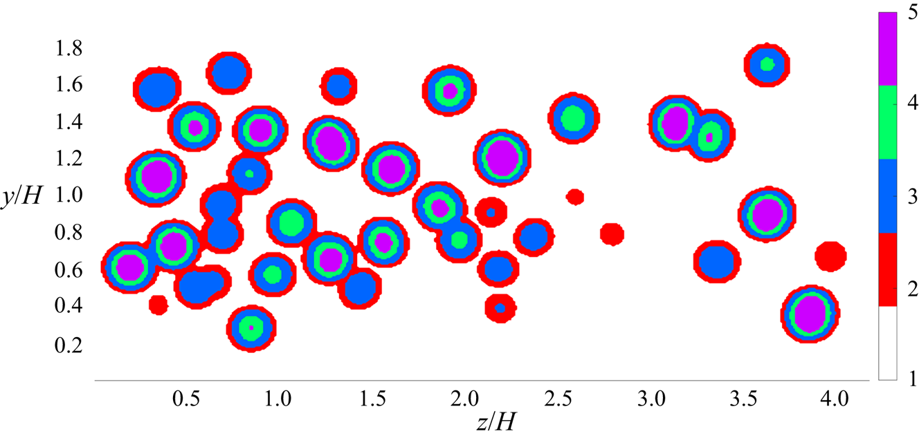
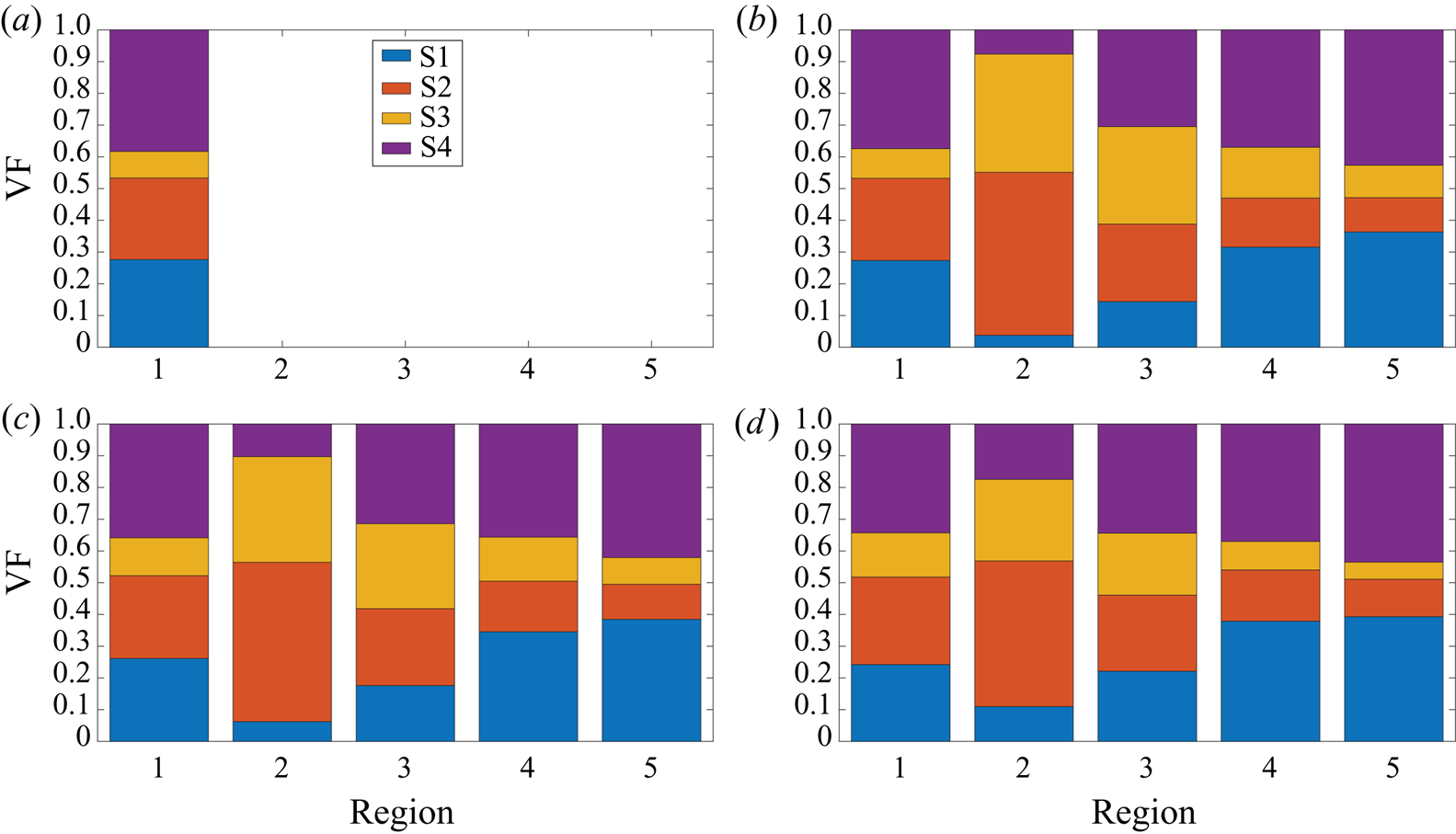
It is instructive to extend the conditional topology evaluation to additional regions in the vicinity of the interface. The meaning of the different regions 1 to 5 can be inferred from figure 11:  $1=\text {liquid bulk}$,
 $2=\text {liquid-interface}$,
 $3=\text {interface}$,
 $4=\text {interface-gas}$,
 $5=\text {gas bulk}$. Those regions are defined by low-pass filtering the volume fraction field
 $\alpha$ and setting threshold values for the filtered field
 $\tilde {\alpha }$ such that the desired width of regions 2, 3 and 4 is obtained (thickness of a few cells in this study). Figure 12 demonstrates a consistent picture in terms of topology distribution for all investigated cases. Apparently, nodal topology S2 is clearly dominant on the liquid side of the interface (region 2) but this is not the case on the gas side of the interface (region 4). Nevertheless, the general increase of nodal topologies, and decrease of focal topologies, from the interior gaseous side to the exterior liquid side is consistent with the analytical findings for laminar creeping flows (figures 3 and 4). Compared to the gas bulk (region 5), the percentage of nodal topology S2 is also increased in region 1, although this region includes the effect of the wall boundary layer which leads to a decrease of S2 as can be seen in figure 10(a,c,e,g). It has already been mentioned in the discussion of figure 7 that the topology distribution in the vicinity of the bubbles in the DNS is not as symmetric as in the analytical solution. Ahead of the bubbles, often the flow is of pure S2 topology type whereas the wake of the bubbles involves a non-negligible share of focal topologies S1 and S4 (due to vortex shedding) besides nodal topology S3. Therefore, S2 and S3 are not equally distributed on the liquid side of the interface (region 2). The generality of these findings must certainly be checked for higher bubble Reynolds numbers and other density/viscosity jumps at the interface.
Spanwise slice of region tags at  $x=L_x/2$ for case ‘high’:
 $1=\text {liquid bulk}$,
 $2=\text {liquid-interface}$,
 $3=\text {interface}$,
 $4=\text {interface-gas}$,
 $5=\text {gas bulk}$.

Topology volume fractions VF conditional on flow regions 1–5 for case ‘single’ (a), ‘low’ (b), ‘medium’ (c), ‘high’ (d).

Regions in the vicinity of the interface, which are of particular importance regarding the sub-grid modelling of two-phase flows, show a clearly different behaviour depending on the phase. A different scaling of velocity variance components on both sides of the interface is also reported in Lakehal (Reference Lakehal2018). Since other quantities relevant to modelling, e.g. the dissipation of turbulent kinetic energy, are likely to show a similar degree of asymmetry with respect to both sides of the interface, a potential sub-grid model must be able to account for this difference. This statement holds true at least if there is a strong coupling between both phases. In other situations, e.g. involving a stronger density jump at the interface (similar to free surface flows), it is probably sufficient to correctly reproduce the behaviour of the heavier phase due to its higher inertia. For the flow conditions considered by Fulgosi et al. (Reference Fulgosi, Lakehal, Banerjee and De Angelis2003), including only mild interface deformations, the lighter phase has been shown to perceive the interface like a solid surface (wall-interface analogy). Accordingly, the topology volume fractions in region 4 in figure 12 are similar to the near-wall distribution in figure 10(a,c,e,g).
4.4. Joint probability of the second and third invariant
To account for the different scale disparity of the second and third invariants, these quantities are normalized by their standard deviation first, i.e.  $Q^*=Q/sd(Q)$ and
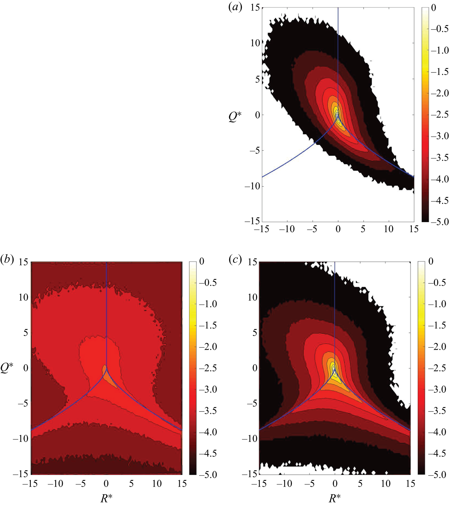
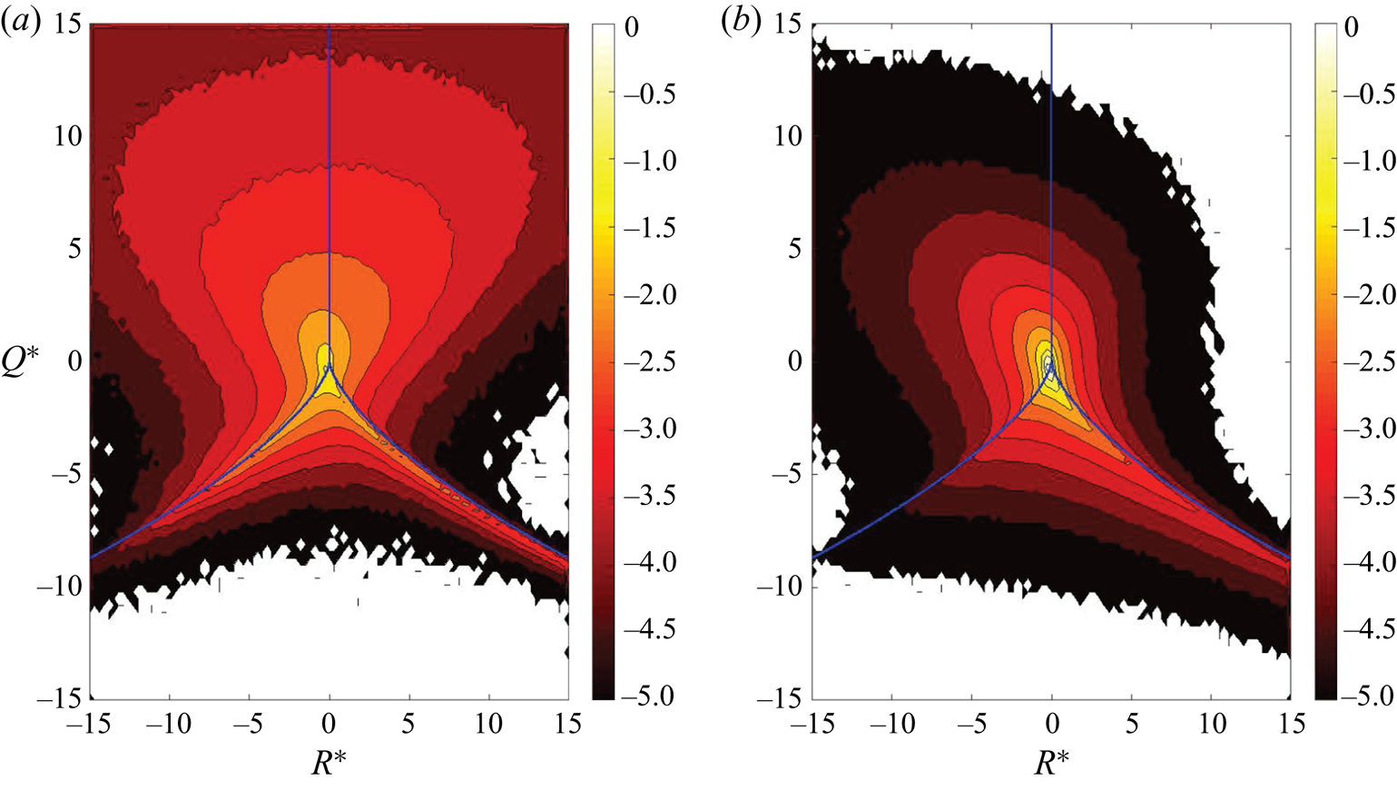
 $R^*=R/sd(R)$, before constructing their joint probability density function. Due to the monotonic behaviour demonstrated earlier, only the extreme cases ‘single’ and ‘high’ are examined in figure 13. Note that the gaseous and liquid phases of both cases are normalized by the standard deviations of the single-phase case to allow for a direct comparison with each other. The typical teardrop shape, well known from the literature (Blackburn et al. Reference Blackburn, Mansour and Cantwell1996; Chong et al. Reference Chong, Soria, Perry, Chacin, Cantwell and Na1998; Chacin & Cantwell Reference Chacin and Cantwell2000), appears very clearly for the single-phase flow. The visual impression of highest population in the S4 quadrant and lowest population in the S3 quadrant matches the calculated topology volume fractions in figure 12. The shape of the joint probability density function, including the apparent accumulation at the topology borders
 $r_{1a}$ and
 $r_{1b}$, for the liquid phase of case ‘high’ is in agreement with the topology analysis on bubble-induced turbulence by Hasslberger et al. (Reference Hasslberger, Klein and Chakraborty2018). Compared to the single-phase flow, an elevated probability of finding nodal topologies S2 and S3 can clearly be discerned, which has already been discussed earlier by means of the corresponding volume fractions. It is worthwhile to recall that the strongest Reynolds stress and turbulent kinetic energy generating events occur where the discriminant of the velocity-gradient tensor, (2.5), has a rapid change of sign (i.e. near the topology borders just mentioned) as indicated by Chacin & Cantwell (Reference Chacin and Cantwell2000). In the gaseous phase of case ‘high’, the shape of the joint probability density function is also somewhat skewed (in the same direction as for the typical single-phase teardrop shape), which is not surprising since both phases are coupled via the deforming interface. However, the scale disparity of
 $Q^*$ and
 $R^*$ is clearly different in both phases. Most prominently, the gaseous phase shows a tendency for higher
 $Q^*$ values, indicating strong vortical motion (either vortex compression or vortex stretching), which is consistent with the observation of a dominant torus-like ring vortex. It can be concluded that the invariant behaviour in both phases is quite different, which is reflected by the different flow topology distributions.
Joint probability density function with common logarithmic scale of the normalized second invariant  $Q^*$ and third invariant
 $R^*$ conditional on the gas phase (b) and liquid phase (a,c) for case ‘single’ (a) and case ‘high’ (b,c). The blue lines indicate the topology borders
 $r_{1a}$,
 $r_{1b}$ and
 $r_2$ according to § 2.

4.5. Size distribution of coherent structures
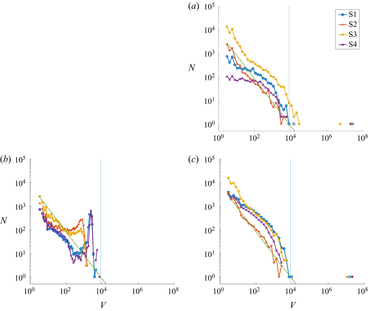
A flood-fill algorithm is applied to determine the size distribution of the topology islands, i.e. coherent structures. Cells of the same topology are considered as connected if they share a common cell face, i.e. each cell not residing at the domain boundary exhibits six potential neighbours. The size range is partitioned into 50 exponentially sized bins to account for the exponential character of the size distribution. The minimum island size is limited to three cells in order to exclude single- and double-cell islands which are likely to be influenced by numerical effects. In figure 14,  $N$ represents the number of topology islands of a certain normalized size
 \begin{equation} V=V^*/({\rm \Delta} x {\rm \Delta} y {\rm \Delta} z), \end{equation}
where  $V^*$ is the actual topology island volume. Apart from very few outliers, i.e. large islands around
 $V\approx 10^7$ at occurrence
 $N=1$, the size distribution
 $N(V)$ in the liquid phase follows roughly a linear trend in the log–log diagram, which suggests a power law like relationship. According to a simple model developed in Hasslberger et al. (Reference Hasslberger, Ketterl, Klein and Chakraborty2019a) (dashed green line in figure 14), the topology size spectrum in the continuous liquid phase can be approximated with reasonable accuracy by
 \begin{equation} N(V)=V_{max} V^{-1}, \end{equation}
where  $V_{max}=(4/3){\rm \pi} (d_b/2)^3/({\rm \Delta} x {\rm \Delta} y {\rm \Delta} z)$ is the corresponding measure of the dominant length scale, i.e. the normalized bubble volume in this case. The model assumes a continuous cascade process ranging from the largest flow structures (approximately at the bubble size) to the smallest identifiable structures on the dissipation level. Figure 6 already demonstrated qualitatively that bubbles are acting as mixing elements and fragment the large topology islands in the bulk of the channel. This fact is obviously reflected in the size distribution: the right end of the liquid spectrum is shifted to somewhat smaller values in the two-phase case compared to the single-phase case (note the logarithmic scale). Apart from the outliers (which are above the cascade range considered), all scales of motion are below the bubble size. Furthermore, it is clear that only coherent structures smaller than the bubble volume, represented by the vertical blue line in figure 14, can exist in the gaseous phase. Note also the distinct size distribution peaks somewhat below the bubble volume. The biggest focal topologies (S1, S4) appear to be larger than the biggest nodal topologies (S2, S3) inside the bubbles, which is also consistent with the analytical findings for laminar creeping flows (figures 3 and 4). The non-monotonic topology size spectrum in the gaseous phase is apparently not described by the simple model (4.2) assuming a continuous cascade process because the flow inside the bubbles is rather dominated by a large torus-like ring vortex. However, for comparably small topology volumes, even the gaseous phase follows the trend predicted by the simple model. In this context, it is interesting to note the increasing separation of nodal and focal topologies towards smaller topology volumes, which can be seen clearly for the single-phase case but is less pronounced for the two-phase case. It seems reasonable that nodal topologies, characterized by dissipation dominating over enstrophy (2.9), are the prevalent flow type for the smallest identifiable structures on the level where kinetic energy dissipates to internal energy. The observed behaviour might be an indication that the turbulence dissipation range is shifted/extended to smaller length scales in two-phase flows when compared to single-phase flows.
Size distribution of connected topology structures conditional on the gas phase (b) and liquid phase (a,c) for case ‘single’ (a) and case ‘high’ (b,c). The vertical blue line represents the bubble volume and the dashed green line represents a simple model (4.2) of the topology size spectrum.

4.6. Influence of the viscosity ratio
Although  $\mu _l / \mu _g = 20$ (thus
 $\nu _l / \nu _g = 1$) is a more realistic set-up for real-world applications, another simulation with
 $\mu _l / \mu _g = 1$ (thus
 $\nu _l / \nu _g = 0.05$) has been performed for the case with the highest bubble count to check upon the influence of the viscosity ratio. It should be kept in mind that a change of
 $\nu _g$ has an influence on both the smallest possible turbulent structures (Kolmogorov length scale
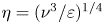 $\eta =(\nu ^3/\varepsilon )^{1/4}$) as well as the boundary layer thickness
 $\delta \propto \sqrt {\nu /U}$ on the gaseous side of the interface. Comparison by means of a turbulent Reynolds number defined as
 \begin{equation} Re_t = \frac{\sqrt{\langle (u_x - \langle u_x \rangle_{l,g})^2 \rangle_{l,g}} \,d_b}{\nu_{l,g}} \end{equation}
yields  $Re_{t,g} \approx 108.3$ and
 $Re_{t,l} \approx 53.1$ for
 $\mu _l / \mu _g = 20$ whereas it yields
 $Re_{t,g} \approx 3.6$ and
 $Re_{t,l} \approx 52.6$ for
 $\mu _l / \mu _g = 1$. These considerations suggest a much less turbulent, possibly quasi-laminar, behaviour within the bubbles for
 $\mu _l / \mu _g = 1$. Indeed, it can be seen from the spanwise (figure 15) and axial slices (figure 16) of the vorticity magnitude and the corresponding topology fields for
 $\mu _l / \mu _g = 1$ that the flow structure in the gaseous phase is much more regular when compared to figures 5, 6 and 7 for
 $\mu _l / \mu _g = 20$. In figure 16, many bubbles can be found showing not only the same sequence of topologies in main flow direction, i.e. S2–S4–S1–S3, but also very similar shapes of the topology regions as compared to the analytical solution for
 $\mu _l / \mu _g = 1$ in figure 18. Another strong similarity concerns the distinct vorticity peaks (torus-like ring vortex) in the vicinity of the interface at an inclination of 90 degrees with respect to the main flow direction which can be found in the DNS (figure 16) as well as the analytical solution (figure 17). It is also interesting to study the viscosity ratio effect by means of the joint probability density function of the normalized second and third invariants of the velocity gradient tensor. Figure 19 for
 $\mu _l / \mu _g = 1$ shall therefore be compared to figure 13 for
 $\mu _l / \mu _g = 20$. The behaviour in the liquid phase seems to be largely unaffected by the change of
 $\mu _g$, which is consistent with the limited response of
 $Re_{t,l}$. In contrast, the behaviour in the gaseous phase changes significantly. The skewed shape of the joint probability density function (in the same direction as for the typical single-phase teardrop shape) in the turbulent case of
 $\mu _l / \mu _g = 20$ practically disappears in the quasi-laminar case of
 $\mu _l / \mu _g = 1$. The volume fractions of nodal topologies S2 and S3 as well as focal topologies S1 and S4 are quite similar. As Hasslberger et al. (Reference Hasslberger, Marten and Klein2019b) showed, a symmetric shape of the joint probability distribution with respect to the axis
 $R=0$ also occurs for the analytical solution for laminar creeping flows.
Spanwise slices of vorticity magnitude 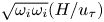 $\sqrt {\omega _i \omega _i} (H/u_\tau)$ (a) and the corresponding topology field (b) at
 $x=L_x/2$ for case ‘high’ with
 $\mu _l / \mu _g = 1$. Interface coloured white.

Axial slices of the first half of the channel showing the vorticity magnitude 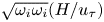 $\sqrt {\omega _i \omega _i} (H/u_\tau)$ (a) and the corresponding topology field (b) at
 $z=L_z/2$ for case ‘high’ with
 $\mu _l / \mu _g = 1$. The main flow direction is from top to bottom. Interface coloured white.

Axisymmetric analytical solution: plane-normal vorticity component  $\omega _z (d_b/u_{x,rel})$ for
 $\mu _l / \mu _g = 1$ with far-field (a) and near-field (b) boundary conditions. The main flow direction is vertical. The green and black lines indicate the interface and the zero-vorticity iso-contour, respectively.

Axisymmetric analytical solution: flow topologies for  $\mu _l / \mu _g = 1$ with far-field (a) and near-field (b) boundary conditions. The main flow direction is from top to bottom and the green line indicates the interface.

Joint probability density function with common logarithmic scale of the normalized second invariant  $Q^*$ and third invariant
 $R^*$ conditional on the gas phase (a) and liquid phase (b) for case ‘high’ with
 $\mu _l / \mu _g = 1$. The blue lines indicate the topology borders
 $r_{1a}$,
 $r_{1b}$ and
 $r_2$ according to § 2.

The above discussion on the generally different flow behaviour in both phases is supposed to draw attention to the correct interpretation of measurements in experiments or simulations. It is likely that, in unconditional flow measurements, the different turbulence levels in the continuous and dispersed phase are masking each other. A clearer picture can be obtained by evaluating statistics in a phase-conditional manner, as is done in this work. The observed limited change of the liquid flow in response to variations in the gaseous flow is to be expected for water–air like density ratios of the order of  $10^3$ (similar to free surface flows) but this is not obvious for a lower density ratio of 20 (as investigated here) where the coupling between both phases is generally stronger.
5. Concluding remarks
In general, the inclusion of bubbles has a strong influence on the flow characteristics, depending on the (local) void fraction. The fact that bubbles are acting as mixing elements is likely to have a strong impact on technical applications regarding the efficiency of heat and mass transfer between both phases.
Several similarities (e.g. dominance of focal topologies inside the bubbles, vorticity distribution inside and in the vicinity of the bubbles, scale disparity of the second and third invariants in their joint probability density functions) with an analytical solution for laminar creeping flows have been observed although the flow is turbulent in the present configuration. The distribution of focal and nodal topologies in the gaseous phase is also very similar to analytically predicted reference values (by two independent approaches in the literature, one assuming a symmetric population in the invariant space and one assuming creeping flow), i.e. 40 % for focal topologies S1/S4 and 10 % for nodal topologies S2/S3. These analogies are particularly obvious for a dynamic viscosity ratio of unity for which a quasi-laminar flow structure emerges inside the bubbles.
No clear analogy can be discerned in terms of the global effects of bubble inclusion and wall confinement on flow topologies. At the cost of both focal topologies, the share of both nodal topologies in the bulk part of the liquid carrier phase clearly increases due to the inclusion of bubbles. In contrast, especially nodal topology S2 decreases and focal topology S1 increases towards the rigid walls until the viscous sublayer is reached. In terms of the near-wall behaviour, it seems also necessary to distinguish the different regions of the boundary layer, i.e. the viscous sublayer, the buffer layer and the region where the logarithmic scaling holds. It can be concluded that the inclusion of bubbles results in a partial shift from focal to nodal flow character whereas the share of stable and unstable flow types remains fairly constant. Remarkably, the share of stable and unstable topologies is approximately 50 % on average, without or with bubbles and in both phases. This finding might be valuable for a unified description of such flows.
Regions in the vicinity of the phase interface, which are of particular importance regarding the sub-grid modelling of two-phase flows, show a clearly different behaviour depending on the phase: strain dominated on the liquid side of the interface, vorticity dominated on the gas side of the interface. Since other quantities relevant to modelling, e.g. the dissipation of turbulent kinetic energy, are likely to show a similar degree of asymmetry with respect to both sides of the interface, a potential sub-grid model must be able to account for this difference.
Regarding the size distribution of coherent structures in the liquid carrier phase, a power law based model developed earlier in the literature approximates the measured topology size spectrum with reasonable accuracy. In the gaseous dispersed phase, a non-monotonic size spectrum has been observed instead which cannot be reproduced by the simple model.
In this present work, the configuration set-up and the fluid properties have been chosen such that the bubbles tend to reside in the core of the channel. The effects of walls and bubbles on turbulent flow structures can consequently be distinguished from each other. In future work, it might be interesting to extend the analysis to scenarios where the bubbles penetrate more deeply into the wall boundary layer. It is yet unclear how this affects the development of coherent structures and corresponding global measures like the wall shear stress. Despite increasing computational cost, it would be worthwhile to repeat the analysis also for higher (bubble) Reynolds numbers.
Acknowledgements
Support by the German Research Foundation (Deutsche Forschungsgemeinschaft – DFG, GS: KL1456/4-1) is gratefully acknowledged. Part of this work was carried out on the Dutch national e-infrastructure with the support of the SURF Cooperative. The Netherlands Organization for Scientific Research (NWO) is gratefully acknowledged for granting access to national supercomputer facilities.
Declaration of interests
The authors report no conflict of interest.
Appendix
To highlight a different aspect of the comparison in § 4.3, figure 20 shows an alternative arrangement of the data already shown in figure 10. Figure 20 reveals fairly monotonic changes in topology volume fractions with increasing void fraction, i.e. bubble number (cases single, low, medium, high):
(i) S1 (focal, unstable): increase in the gas, decrease in the liquid;
(ii) S2 (nodal, unstable): marginal change in the gas, increase in the liquid;
(iii) S3 (nodal, stable): decrease in the gas, increase in the liquid;
(iv) S4 (focal, stable): marginal change in the gas, decrease in the liquid.
Wall-normal profiles of slice-based topology volume fractions VF conditional on the gas phase (a,c,e,g) and liquid phase (b,d,f,h) for flow topology S1 (a,b), S2 (c,d), S3 (e,f), S4 (g,h).