1. Introduction
The present study follows a previous weakly nonlinear analysis of wrinkled shocks describing the formation of triple points (Mach stems) propagating along the front of strong shock waves in the Newtonian limit (Clavin Reference Clavin2013; Denet et al. Reference Denet, Biamino, Lodato, Vervisch and Clavin2015). Here a numerical study is performed concerning a moderately weak shock in air, reflected from a sinusoidal wall of small amplitude (incident Mach number 1.5, wall amplitude and wavelength 1 mm and 20 mm, respectively). The linear stability analysis of planar shocks has a long history starting with the works of Lighthill (Reference Lighthill1949, Reference Lighthill1950) and Freeman (Reference Freeman1955), who showed a relaxation which follows a power law. The normal mode analysis cannot capture such a relaxation rate and leads to neutral modes that are non-radiating (see D’Yakov Reference D’Yakov1954; Kontorovich Reference Kontorovich1957; Clavin & Williams Reference Clavin and Williams2012). In these early works, little attention was paid to the formation of triple points that were, indeed, observed in the pioneering experiments of Lapworth (Reference Lapworth1959) and of Briscoe & Kovitz (Reference Briscoe and Kovitz1968) concerning shock waves reflected from a wavy wall. The analytical description of such singular points requires nonlinear analyses. The cellular structure of detonations was the motivation behind the pioneering nonlinear analysis of Majda & Rosales (Reference Majda and Rosales1983). In the present study, attention is focused not only on the spontaneous formation of triple points on the shock waves alone, their interactions and their dynamics, but also on the flow pattern generated in the shocked gas. One of the questions that is addressed is to know to what extent the transverse motion of the triple points, once formed, is influenced by the complex flow generated in the shocked gas. The configuration is selected so as to match some existing experimental data and also to obtain a sufficiently smooth initial deformation of the shock front. Under these conditions, the spontaneous formation of triple points on the shock front can be triggered and thoroughly described. The hope is that, sufficiently far from the wall, the dynamics of the reflected shock is mainly controlled by the intrinsic nonlinear dynamics of a freely propagating shock wave.
The study of the formation of triple points on pure shocks is useful for improving our understanding of the cellular structure of weakly unstable detonations against transverse perturbations. Previous weakly nonlinear analyses (Clavin & Denet Reference Clavin and Denet2002; Clavin Reference Clavin2013) have shown that the main characteristics of the cellular pattern of detonations that are weakly unstable to multi-dimensional disturbances are associated with nonlinear mechanisms which are inherent to the leading shock. The rate of heat release is responsible for the linear instability that feeds the cellular pattern. It selects the range of unstable wavelengths and the cell size is directly related to the detonation thickness. However, the heat release does not play an important role in the formation and the dynamics of the triple points (or lines) propagating on the leading shock wave. This is true only near the multi-dimensional instability threshold of detonations. Experiments and numerical investigations show that the situation is much more complex in strongly unstable detonations. Hot pockets of reactive mixture explode in the shocked gas and a Kelvin–Helmholtz instability of the contact discontinuity line (shear wave) develops (see the work of Radulescu et al. Reference Radulescu, Sharpe, Lee, Kiyanda, Higgins and Hanson2005, Mazaheri, Mahmoudi & Radulescu Reference Mazaheri, Mahmoudi and Radulescu2012 and Mahmoudi & Mazaheri Reference Mahmoudi and Mazaheri2015 for example). The complexity comes from the fact that a one-dimensional instability mechanism (secondary bifurcation of pulsating detonations) is superimposed on the multi-dimensional instability. This phenomenon, in particular, deserves further theoretical analysis that is outside the scope of the present study. We will come back to this point in the conclusion.
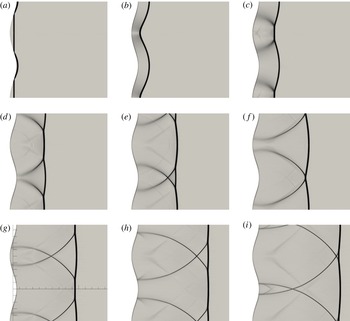
Time frames of the evolution of the shock after reflection. (a)
 $0~{\rm\mu}\text{s}$
, (b)
 $10~{\rm\mu}\text{s}$
, (c)
 $20~{\rm\mu}\text{s}$
, (d)
 $30~{\rm\mu}\text{s}$
, (e)
 $40~{\rm\mu}\text{s}$
, (f)
 $50~{\rm\mu}\text{s}$
, (g)
 $60~{\rm\mu}\text{s}$
, (h)
 $70~{\rm\mu}\text{s}$
, (i)
 $80~{\rm\mu}\text{s}$
. The reference marks in (g) are 2 mm spaced.

As anticipated in the theoretical analysis (Clavin Reference Clavin2013), a long-lived pattern of triple points, similar to that observed in cellular detonations, develops on an inert shock starting from a smooth sinusoidal disturbance of the front. This has been recently confirmed by both a preliminary numerical simulation and a shock tube experiment (Denet et al. Reference Denet, Biamino, Lodato, Vervisch and Clavin2015), performed using an existing experimental set up devoted to multiple investigations (Jourdan et al. Reference Jourdan, Houas, Schwaederlé, Layes, Carrey and Diaz2004). The present numerical study aims to reproduce this experiment using direct numerical simulation (DNS) in order to clarify the nature of the cellular front and of the flow associated with the interaction of the transverse travelling waves propagating in the shocked gas in the form of very thin fronts. These flow patterns have not yet been investigated and only the transverse shock waves have been visualized in the experiment via Schlieren photography.
The interaction between obstacles and shock waves has been the subject of many studies on shock reflection in inert flows (see Izumi, Aso & Nishida Reference Izumi, Aso and Nishida1994; Gelfand et al. Reference Gelfand, Khomik, Bartenev, Medvedev, Grönig and Olivier2000; Kowalczyk, Płatkowski & Waluś Reference Kowalczyk, Płatkowski and Waluś2000; Ben-Dor Reference Ben-Dor2007; Skews & Kleine Reference Skews and Kleine2007; Taieb, Ribert & Hadjadj Reference Taieb, Ribert and Hadjadj2010; Shadloo, Hadjadj & Chaudhuri Reference Shadloo, Hadjadj and Chaudhuri2014, and references therein) and also in the context of detonation establishment of Mach stems and detonation re-initiation (see Bhattacharjee et al. Reference Bhattacharjee, Lau-Chapdelaine, Maines, Maley and Radulescu2013). In contrast to these studies, the amplitude of the wavy wall in the present numerical study is so small that the focusing phenomenon is limited to producing an increase of pressure in the concave part of the wall, which can be considered as a shallow reflector (Kowalczyk et al. Reference Kowalczyk, Płatkowski and Waluś2000). As a consequence, the reflection on the wavy wall is regular and no transition to Mach reflection is observed at the wall. As shown in figure 1, the shock front looks smoothly perturbed just after reflection and no triple points are observed at first. A few micro-seconds after reflection, triple points are formed spontaneously on the reflected shock front. These points and the relevant subsequent interactions are later responsible for the establishment, on the reflected shock front and the downstream shocked gases, of a long-lived pattern which appears similar to that typically observed in cellular detonations. Sufficiently far from the wavy wall, the flow patterns in the inert shocked gas of the reflected shock bear some relatively marked resemblance to the burnt gas flow of the cellular detonation front observed in previous two-dimensional numerical studies (e.g. Taki & Fujiwara Reference Taki and Fujiwara1981; Kailasanath et al. Reference Kailasanath, Oran, Boris and Young1985; Guirguis, Oran & Kailasanath Reference Guirguis, Oran and Kailasanath1986; Bourlioux & Majda Reference Bourlioux and Majda1992; Oran et al. Reference Oran, Weber, Stefaniw, Lefebvre and Anderson1998; Gamezo, Desbordes & Oran Reference Gamezo, Desbordes and Oran1999). The resemblance is even more striking in the case of small heat release (cf. Bourlioux & Majda Reference Bourlioux and Majda1992, §3, case A).
The two-dimensional compressible flow generated after the shock reflection on the wavy wall is strongly unsteady and very complicated. It will be shown that the salient features of the instantaneous streamline patterns consist of a few standard flows associated with critical points. Critical points have been identified for a long time in the ‘phase-space’ of the solutions of autonomous ordinary differential equations. The concept has been developed in fluid mechanics more recently, in the 1960s, for analysing three-dimensional incompressible flows (see Perry & Chong Reference Perry and Chong1987; Chong, Perry & Cantwell Reference Chong, Perry and Cantwell1990, and references therein). In the frame attached to a critical point, the flow velocity is zero and the streamline slope is indeterminate. An asymptotically exact solution of the Navier–Stokes equations is obtained around each critical point using Taylor series. The critical points are classified into categories, according to the value of the invariants of the velocity gradient tensor. For example, this approach has been successful in exhibiting the physical picture of turbulent boundary layers (Chacin & Cantwell Reference Chacin and Cantwell2000). Our purpose is not to develop the theory of critical points in two-dimensional compressible flows: that has not yet been done to the best of our knowledge. Our purpose is limited to showing how such short-lived pieces of singular flow appear intermittently in the unsteady compressible flow and control the topology of the instantaneous streamline patterns.
The paper is organized as follows. The parameters of the numerical computation are presented in § 2 and the results from the DNS are compared to the available experimental data in § 3. The structure and the dynamics of the triple points propagating on the leading front is thoroughly analysed in § 4. The flow topology and the relevant patterns are analysed in § 5. Finally, the results are discussed in § 6. For completeness, some details regarding the numerical solver used to perform DNS are provided in appendices A–C.
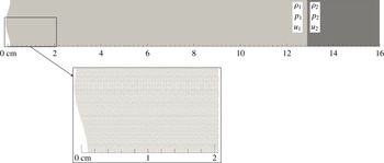
View of the computational domain coloured by the initial density field.

2. Methodology
The interaction between a shock and a sinusoidal wall is simulated numerically in a two-dimensional geometry. In order to obtain the most detailed description of the flow field generated after the shock reflection, a DNS is performed using the high-order spectral difference (SD) method (Kopriva & Kolias Reference Kopriva and Kolias1996; Jameson Reference Jameson2010) to solve the compressible Navier–Stokes equations. The SD scheme, in particular, enables arbitrary high-order computations on unstructured meshes and provides high resolution of the flow features while introducing minimal numerical dissipation. The adopted shock capturing methodology is designed to provide sub-cell resolution of the flow discontinuities through a high-order dissipation term (Persson & Peraire Reference Persson and Peraire2006; Persson Reference Persson2013). As a result, detrimental numerical damping of the instabilities of the shock front is minimized. Details regarding the numerical method and the shock capturing approach, which, in particular, features a novel auto-calibration algorithm, are reported for completeness in appendices A and B. It is worthwhile stressing that the present setup is characterized by a large separation of scales. In the reflected shock configuration, the velocities of the complex flow pattern in the shocked gas are orders of magnitude smaller than the incoming velocity. Such flows are difficult to detect in an experiment and challenging to numerically reproduce with a sufficient level of detail.
The Navier–Stokes equations – augmented with a localized artificial viscosity term for shock-capturing purposes – are integrated over a computational domain 16 cm long and 2 cm high with
 $600\times 90$
unstructured quadrilateral elements, whose typical dimension is about
 $250~{\rm\mu}\text{m}$
. The reported computations are fifth-order in space and time. Accordingly,
 $5\times 5$
solution points are used in each element and the actual spatial resolution can be estimated to be of the order of 50
 ${\rm\mu}\text{m}$
. The total number of degrees of freedom is
 $1.35\times 10^{6}$
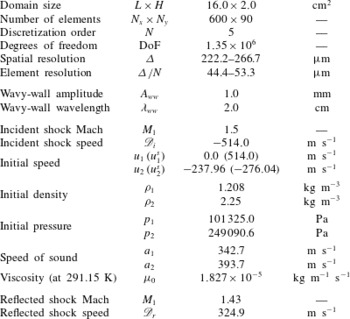
. The left no-slip wall has a sinusoidal shape with 1 mm amplitude and 2 cm wavelength. The right boundary is set as an inflow, whose parameters correspond to the compressed (shocked gases) state of the incident shock (see below), whereas the top and bottom boundaries are set as periodic. The computational domain is depicted in figure 2, where a close-up of the bottom left part is included to better visualize the size of the elements. The mesh dimension and resolution, and the initial flow parameters discussed below, are summarized in table 1.
Mesh parameters and flow setup. Velocities are indicated in the laboratory reference frame; relevant values in the shock reference frame are indicated in parentheses.

All the parameters of the simulations have been selected to match the experiment of Biamino reported in Denet et al. (Reference Denet, Biamino, Lodato, Vervisch and Clavin2015). In this experiment, a vertical planar shock propagating at a velocity
 $\mathscr{D}_{i}=514~\text{m}~\text{s}^{-1}$
(and Mach number 1.5) in air at rest is reflected from a wavy wall. The velocity of the reflected (quasi-planar) shock is
 $\mathscr{D}_{r}=325~\text{m}~\text{s}^{-1}$
in the laboratory frame. The propagation velocity relative to the upstream gas, which is set into motion at a speed of
 $239~\text{m}~\text{s}^{-1}$
by the incident shock before reflection, is
 $325+239=564~\text{m}~\text{s}^{-1}$
. Whence, the corresponding Mach number of the reflected shock is measured equal to 1.43. The front of the reflected shock features triple points moving in both transverse directions at a vertical velocity of about
 $310~\text{m}~\text{s}^{-1}$
; see figure 3(a,c,e). The trajectories of these triple points form a diamond-like pattern similar to the markings left by a detonation on soot-coated foils at the walls of the tube.
Regarding the numerical setup, typical properties of air are used in the simulation, hence the specific heat ratio
 ${\it\gamma}$
is set equal to 1.4, the Prandtl number is set equal to 0.72 and the dynamic viscosity is computed by the Sutherland’s law:
 ${\it\mu}(T)={\it\mu}_{0}\left(T/T_{0}\right)^{3/2}(T_{0}+T_{S})/(T+T_{S})$
with
 ${\it\mu}_{0}=1.827\times 10^{-5}~\text{kg}~\text{m}^{-1}~\text{s}^{-1}$
,
 $T_{S}=120$
K and
 $T_{0}=291.15~\text{K}$
. Using the same notation as in figure 2, the initial pressure and density of the gas initially at rest are
 $p_{1}=101\,325~\text{Pa}$
and
 ${\it\rho}_{1}=1.208~\text{kg}~\text{m}^{-3}$
. The pressure and density of the compressed gas of the incident shock,
 $p_{2}=249\,090.6~\text{Pa}$
and
 ${\it\rho}_{2}=2.25~\text{kg}~\text{m}^{-3}$
, are obtained from the Rankine–Hugoniot conditions (see appendix C) for a propagation Mach number
 $M_{1}\equiv \mathscr{D}_{i}/a_{1}=1.5$
where
 $a_{1}=({\it\gamma}p_{1}/{\it\rho}_{1})^{1/2}\approx 342.68~\text{m}~\text{s}^{-1}$
is the speed of sound. According to the Hugoniot relations, the velocity of the compressed gas relative to the shock is
 $u_{2}^{s}=\mathscr{D}_{i}{\it\rho}_{1}/{\it\rho}_{2}=276.04~\text{m}~\text{s}^{-1}$
corresponding to a velocity in the laboratory frame
 $u_{2}\equiv u_{2}^{s}-\mathscr{D}_{i}=-237.96~\text{m}~\text{s}^{-1}$
. In the computation, these values for
 $p_{2}$
,
 ${\it\rho}_{2}$
and
 $u_{2}$
are set as the inlet parameters so as to prevent any perturbation to the flow at the right boundary. As shown in figure 2, the incident shock is initially located at 12.88 cm from the wavy wall – whose position is hereinafter identified with the location of its mid-plane – and left to evolve for a total time of
 $700~{\rm\mu}\text{s}$
, and a total of 350 frames, one every
 $2~{\rm\mu}\text{s}$
, have been extracted from the simulation. At the speed of 514
 $\text{m}~\text{s}^{-1}$
, it takes about
 $250~{\rm\mu}\text{s}$
for the incident shock to reach the wavy wall. At the end of the computation,
 $450~{\rm\mu}\text{s}$
after the interaction with the wavy wall, the reflected shock is at a distance of 14.62 cm from the wall, corresponding to an average velocity
 $\mathscr{D}_{r}$
of the reflected shock in the laboratory reference frame of about
 $324.9~\text{m}~\text{s}^{-1}$
(
 $\mathscr{D}_{r}=325~\text{m}~\text{s}^{-1}$
in the experiment). The air upstream of the reflected shock has a velocity of
 $237.96~\text{m}~\text{s}^{-1}$
oriented to the left, and the propagation velocity of the reflected shock in the upstream gas at rest is
 $324.9+237.96=562.86~\text{m}~\text{s}^{-1}$
(
 $564~\text{m}~\text{s}^{-1}$
in the experiment). The speed of sound upstream of the reflected shock, where the pressure and density are equal to 249 090.6 Pa and
 $2.25~\text{kg}~\text{m}^{-3}$
, respectively, is
 $({\it\gamma}p/{\it\rho})^{1/2}\approx 393.7~\text{m}~\text{s}^{-1}$
, so that the resulting propagation Mach number of the reflected shock equals 1.43, as reported in the experiment.
3. Comparison to experiments
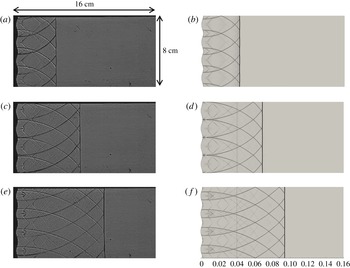
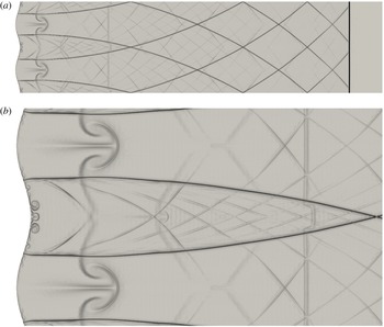
Qualitative comparison between experimental (a,c,e, Denet et al. Reference Denet, Biamino, Lodato, Vervisch and Clavin2015) and numerical (b,d,f). Schlieren images at three different times after reflection.
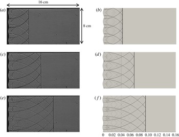
The Schlieren images obtained by the numerical simulation, showing the reflected shock and the transverse waves propagating in the shocked gas, are plotted for comparison in figure 3(b,d,f) for the same instants of time after reflection (120, 200,
 $280~{\rm\mu}\text{s}$
) for which the experimental Schlieren images of Biamino (Denet et al.
Reference Denet, Biamino, Lodato, Vervisch and Clavin2015) are available; see figure 3(a,c,e). The comparison is quite satisfactory.
Also note that, as shown in figure 4, the speed of sound in the shocked gas of the reflected shock wave is not quite uniform; it lies in the range
 $440{-}450~\text{m}~\text{s}^{-1}$
, which is in good agreement with the evaluation of
 $446~\text{m}~\text{s}^{-1}$
obtained by using the Rankine–Hugoniot conditions for a propagation Mach number 1.43 and upstream conditions
 $p=249\,090.6$
Pa and
 ${\it\rho}=2.25~\text{kg}~\text{m}^{-3}$
.
3.1. The spurious weak contact discontinuity
The vertical line which is visible in the computation (see figure 3) at about 4 cm from the sinusoidal wall, is a weak contact discontinuity (or entropy wave) which was generated at the beginning of the computation due to the initial establishment of the resolved shock front from the given (ideal) sharp discontinuity (Rankine–Hugoniot conditions) imposed at the element interfaces. During the first stages of the computation, the numerical scheme reacts to properly resolve such a sharp discontinuity. As a result, during the first few iterations, a right-running very weak acoustic wave and a left-running contact discontinuity are generated. The former leaves the computational domain through the right boundary in about
 $200~{\rm\mu}\text{s}$
as expected, whereas the latter – which corresponds to a jump in the density of about 2.4 % of the density jump of the initial shock – travels toward the wall at the flow velocity of
 $237.96~\text{m}~\text{s}^{-1}$
and later meets the reflected shock front at about
 $106~{\rm\mu}\text{s}$
after reflection. Although the issue could have been avoided by computing the initial solution with an established (namely numerically resolved) shock front extracted from a precursor simulation of a similar steady shock at the same Mach number, this type of initialization was not deemed necessary in the present work. In fact, as can be observed in figures 3 and 5 at the end of the calculation, the strength of this spurious discontinuity is sufficiently low not to significantly perturb the flow and the structures in the shocked gases. This notwithstanding, in order to prevent any influence by this spurious perturbation, the analysis and the quantitative results presented in the next sections are restricted to the first
 $100~{\rm\mu}\text{s}$
after reflection, in other words, approximately
 $6~{\rm\mu}\text{s}$
before the interaction between the reflected shock and the spurious contact discontinuity takes place.
Contour map of the speed of sound at
 $t=280~{\rm\mu}\text{s}$
.

Numerical Schlieren picture of the flow at
 $t=450~{\rm\mu}\text{s}$
(a) and close-up view of the region near the wall (b).

3.2. The transverse velocity of the triple points
The measure of the vertical displacement of the triple points along the lead shock (moving at velocity
 $\mathscr{D}_{r}=325~\text{m}~\text{s}^{-1}$
in the laboratory frame) yields a velocity of about
 $310~\text{m}~\text{s}^{-1}$
. This is again in perfect agreement with what is reported in the experiment.
Following the procedure described below, the subsonic velocity
 $310~\text{m}~\text{s}^{-1}$
is shown to correspond to the supersonic propagation with a Mach number 1.03
 $\pm$
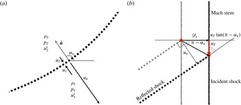
0.02 of the weak transverse shocks that are issued from the triple points and propagate in the shocked gas of the leading shock front (after reflection on the wavy wall); see the Schlieren images. According to the geometrical construction depicted in figure 6(b), the propagation velocity
 $|u_{n}|$
of a planar front, tilted by an angle
 ${\it\alpha}_{n}-{\rm\pi}/2$
(
 ${\it\alpha}_{n}$
is the angle between the horizontal and the normal oriented in the opposite direction to propagation; see figure 6
a), is linked to the vertical velocity
 $|u_{T}|$
of its intersection with a vertical line propagating at the velocity
 $\mathscr{D}_{r}$
by the relation
 $$\begin{eqnarray}|u_{n}|=\left[\mathscr{D}_{r}+|u_{T}|\tan ({\rm\pi}-{\it\alpha}_{n})\right]\cos ({\rm\pi}-{\it\alpha}_{n}),\end{eqnarray}$$
written here for a wave propagating downward with a normal velocity
 $|u_{n}|>\mathscr{D}_{r}$
and with
 ${\it\alpha}_{n}\in [{\rm\pi}/2,{\rm\pi}]$
. For
 $|u_{T}|=310~\text{m}~\text{s}^{-1}$
,
 $\mathscr{D}_{r}=325~\text{m}~\text{s}^{-1}$
and an angle
 ${\it\alpha}_{n}=133.7^{\circ }$
– a value that corresponds to the transverse shock of the triple point on the upper part of figure 7(a) at
 $t=50~{\rm\mu}\text{s}$
– (3.1) yields
 $|u_{n}|=443.2~\text{m}~\text{s}^{-1}$
. The corresponding Mach number is computed from the local sound speed and the normal component of the flow velocity relative to the secondary shock front, as described below.
(a) Schematic representation of a transverse wave front and identification of the relevant quantities. (b) Geometrical construction to obtain the vertical velocity
 $|u_{T}|$
of the triple point from the normal velocity of the reflected shock (transverse wave)
 $|u_{n}|$
and from the horizontal of the lead shock
 $\mathscr{D}_{r}$
, both measured in the fixed referential frame of the laboratory.

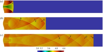
Contours of density at three subsequent instants in time showing the location of the selected points for the analysis of the wave fronts. (a)
 $t=50~{\rm\mu}\text{s}$
, (b)
 $200~{\rm\mu}\text{s}$
,(c)
 $440~{\rm\mu}\text{s}$
.

3.3. The Mach number of the transverse waves
In this section, the flow parameters across the transverse waves, at different locations and instants in time, are analysed in order to establish the propagation Mach number and speed of these waves in the laboratory reference frame.
The normal to the transverse waves
 $\hat{\boldsymbol{n}}$
is obtained by measuring the local peak value of the gradient of density, namely,
 $\hat{\boldsymbol{n}}=\boldsymbol{{\rm\nabla}}{\it\rho}/\Vert \boldsymbol{{\rm\nabla}}{\it\rho}\Vert$
. Hence, by definition,
 $\hat{\boldsymbol{n}}$
is oriented in the direction of increasing density. Given a position vector
 $\boldsymbol{x}$
in the vicinity of a transverse wave, the normal component of the flow velocity
 $\boldsymbol{u}(\boldsymbol{x})$
in the laboratory frame is denoted
 $u\equiv \boldsymbol{u}(\boldsymbol{x})\boldsymbol{\cdot }\hat{\boldsymbol{n}}$
and the normal flow velocity relative to the front is
 $u^{\text{s}}\equiv u-u_{n}$
where
 $u_{n}=-|u_{n}|$
if the direction of propagation is opposite to
 $\hat{\boldsymbol{n}}$
and
 $u_{n}=|u_{n}|$
otherwise. For a shock wave one has
 $u^{s}>0$
. The quantities
 $u$
and
 $u^{s}$
are defined at two points
 $\boldsymbol{x}_{1}$
and
 $\boldsymbol{x}_{2}$
on each side of the front. With reference to the sketch in figure 6(a), the regions 1 and 2 are established such that
 $\hat{\boldsymbol{n}}$
points from 1 (less dense gas) to 2 (dense side), so that the propagation Mach number is
 $$\begin{eqnarray}M_{1}^{\text{s}}\equiv u_{1}^{s}/\sqrt{{\it\gamma}p_{1}/{\it\rho}_{1}}>1,\end{eqnarray}$$
where
 $p_{1}$
and
 ${\it\rho}_{1}$
are obtained from the numerical results. Using the Rankine–Hugoniot conditions in appendix C, the measures of the ratios
 $p_{2}/p_{1}$
or
 ${\it\rho}_{2}/{\it\rho}_{1}$
are expected to give the same propagation Mach number
 $M_{1}^{s}$
. The estimated value is taken equal to the average of those obtained from the pressure and density ratios, respectively, and the relevant errors are indicated in table 2 as
 ${\it\epsilon}_{M_{1}}$
. Using (3.2), the measured value of
 $M_{1}^{s}$
and the speed of sound, can be used to compute the (normal) velocities in the shock reference frame
 $u_{1}^{s}$
and, from mass conservation,
 $u_{2}^{s}={\it\rho}_{1}u_{1}^{s}/{\it\rho}_{2}$
. For a wave front which propagates along the direction
 $\hat{\boldsymbol{n}}$
with velocity
 $u_{n}$
(relative to the laboratory reference frame), the measured values of
 $u_{i}$
and the computed values of
 $u_{i}^{s}$
have to satisfy the equations
 $u_{1}=u_{1}^{s}+u_{n}$
and
 $u_{2}=u_{2}^{s}+u_{n}$
simultaneously. Hence,
 $u_{n}$
is estimated as
 $(u_{1}+u_{2}-u_{1}^{s}-u_{2}^{s})/2$
. The relevant accuracy can be evaluated with respect to the obvious identity
 $u_{1}-u_{1}^{s}=u_{2}-u_{2}^{s}$
. This is indicated in table 2 as
 ${\it\epsilon}_{u_{n}}$
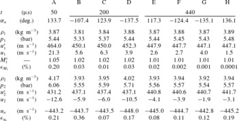
. These checks have been performed at different points of different transverse waves in the shocked gas and at different times with an overall accuracy of the order of 0.4 % or less. The results concerning the eight points indicated in figure 7, where arrows are used to identify the normal
 $\hat{\boldsymbol{n}}$
, are shown in table 2. The Rankine–Hugoniot relations are verified with a good accuracy in the actual measurements, showing that the waves are weak transverse shocks whose propagation Mach number is in the range 1.01–1.05. Using the measured value of
 $|u_{T}|$
of about
 $310~\text{m}~\text{s}^{-1}$
,
 $\mathscr{D}_{r}=324.9~\text{m}~\text{s}^{-1}$
and the angles
 ${\it\alpha}_{n}$
at the points A, D and H – the closest to the triple points – (3.1) can be used to estimate
 $|u_{n}|$
for the aforementioned points and compare with the value obtained from the Rankine–Hugoniot relations (see table 2). A good agreement is obtained with relative errors (not indicated) always smaller than 1.2 %. The negative sign of the values of
 $u_{n}$
indicates that the transverse waves depicted in figure 7 move opposite to the direction of the represented vectors. Hence, the two transverse waves in figure 7(a) (
 $t=50~{\rm\mu}\text{s}$
), which are also shown in the upper part of figure 1(f), move toward each other. A short time later they interact to form a crossing point downstream of the leading shock, as is shown in the upper part of figure 1(g) (
 $t=60~{\rm\mu}\text{s}$
). At any instant in time, the resulting system of transverse weak shocks takes the form of a diamond-like pattern, which is visible in figures 5(a) or 7(c) and which appears quite similar to the arrangement observed in the experiment through Schlieren photography (see figure 3). Notice the small increase of density in the shocked gas of both transverse waves after interaction in figures 7(b) and 7(c). This pattern should not be confused with the one constituted by the trajectories (in the laboratory reference frame) of the triple points of the leading shock. The latter is stationary.
Wave-front parameters. The errors are computed as
 ${\it\epsilon}_{{\it\phi}}=100\times 2|{\it\phi}_{a}-{\it\phi}_{b}|/|{\it\phi}_{a}+{\it\phi}_{b}|$
, where
 ${\it\phi}$
is either
 $M_{1}^{s}$
or
 $u_{n}$
and subscripts
 $a$
and
 $b$
indicate two relevant measures.

4. Structure and dynamics of the triple points
The flow field is strongly unsteady and extremely complex, as we shall see in § 5. On the contrary, the dynamics of the triple points on the leading shock is relatively simple and regular. In this section, attention is focused on the structure and dynamics of the triple points colliding on the leading shock.
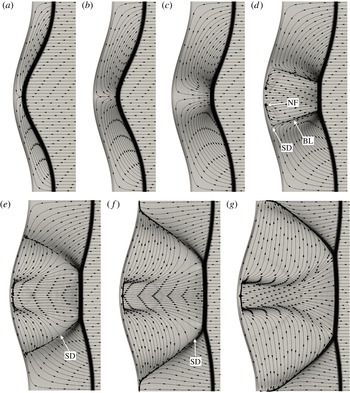
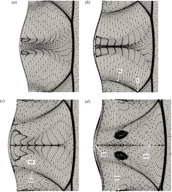
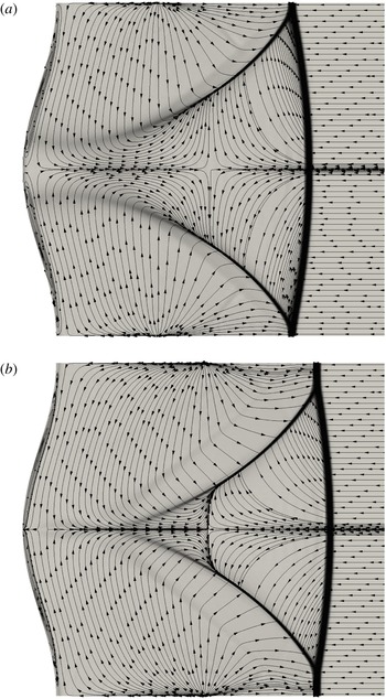
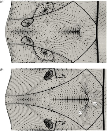
Time evolution of the flow streamlines and Schlieren image after reflection (SD, saddle point; BL, bifurcation line; NF, node-focus). (a)
 $t=6~{\rm\mu}\text{s}$
, (b)
 $10~{\rm\mu}\text{s}$
, (c)
 $14~{\rm\mu}\text{s}$
, (d)
 $18~{\rm\mu}\text{s}$
, (e)
 $22~{\rm\mu}\text{s}$
, (f)
 $26~{\rm\mu}\text{s}$
, (g)
 $30~{\rm\mu}\text{s}$
.

4.1. The formation of singularities in a finite time
The spontaneous formation of singularities in the slope of the shock front is clearly shown in figure 1, where close-ups of the region in the vicinity of the wavy wall are depicted at different instants in time just after the impact of the shock wave on the wall. The streamlines are shown in figure 8(a–d), where the arrows show the direction of the flow in the laboratory-fixed frame. The reflected shock has a quasi-smooth shape just after reflection. The formation of cusps pointing toward the concave part of the wavy wall is first observed at about
 $12{-}14~{\rm\mu}\text{s}$
on the concave part of the shock front. As seen in figure 1(c), at about
 $20~{\rm\mu}\text{s}$
these singularities have already split into pairs of triple points propagating in opposite directions along the shock front. The triple points subsequently collide for the first time at about
 $50~{\rm\mu}\text{s}$
(cf. figure 1
f). We will come back in § 5 to the formation of triple points and, more specifically, to the corresponding transient flow field in the shocked gas.
The reflection of shock waves on a rigid wall is a well-known problem, which has been extensively studied for a long time (Courant & Friedrichs Reference Courant and Friedrichs1948). The main result is the transition between a regular reflection (two shocks: an incident shock and a reflected shock) for a small angle of incidence to a Mach reflection (Mach stem configuration: three shocks plus a contact line). The critical angle of incidence for transition from regular to Mach reflection over a cylindrical convex surface is typically in the range 30°–40° for shocks in nitrogen at Mach numbers greater than 1.1; the computed critical angle of incidence is about 40° at Mach 1.5 (see Ben-Dor Reference Ben-Dor2007, figure 4.27). In particular, for the sinusoidal wall shape considered here, the wedge angle is easily obtained as
 ${\it\theta}_{w}=90^{\circ }+(180^{\circ }/{\rm\pi})\tan ^{-1}[f^{\prime }(y)]$
, where
 $f^{\prime }(y)$
is the derivative, with respect to the vertical coordinate
 $y$
, of the wall profile
 $f(y)=A_{ww}\cos (2{\rm\pi}y/{\it\lambda}_{ww})$
. For
 $A_{ww}=1$
mm and
 ${\it\lambda}_{ww}=2$
cm, as in the present study, the smallest value of
 ${\it\theta}_{w}$
is 72.6°. Hence, the geometry of the reflector under consideration does not allow the transition to Mach reflection during the whole interaction between the incident shock and the wall. In the short lapse of time during which the impact between the incident shock and the wavy wall takes place, the reflection is regular but the reflected shock and the concave part of the wall are so close that they are difficult to separate in figure 1(a). As already mentioned, the reflected shock front appears to have a smoothly curved profile just after reflection.
4.2. Free-slip versus no-slip conditions at the endwall
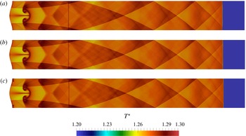
In order to understand whether or not the complex and intermittent flow in the shocked gases is essential to the formation and the dynamics of the triple points, additional computations using the Euler equations (i.e. no viscosity except in the shock tracking region) and Navier–Stokes equations with a free-slip boundary condition at the wall have been performed. In such conditions, the development and subsequent destabilization of the boundary layer at the wall cannot occur. A comparison of the (normalized) temperature maps obtained from inviscid and viscous computations, these last with free- or no-slip boundary conditions, is depicted in figure 9. With the exception of the region close to the wall, no difference is visible in the flow field and in the trajectories of the triple points.
This comparison shows that the dynamics of the cellular shock front is quasi-local, intrinsic to that of the triple points and independent of the flow field downstream of the shock. This flow field is a consequence of the motion of the triple points and, sufficiently far from the endwall, has no real retro-action on the dynamics of the cellular shock front.
Contour maps of normalized temperature at
 $t=440~{\rm\mu}\text{s}$
. (a) Euler equations, (b) Navier–Stokes equations, free-slip wall condition, (c) Navier–Stokes equations, no-slip wall condition.

4.3. Mach stems and slip lines
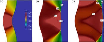
Contour maps of normalized temperature after reflection: IS, incident shock; MS, Mach stem; RS, reflected shock; SL, slip line. (a)
 $t=14~{\rm\mu}\text{s}$
, (b)
 $30~{\rm\mu}\text{s}$
, (c)
 $38~{\rm\mu}\text{s}$
.

The triple points observed on the cellular shock wave have the same typical three-shock configuration as the Mach reflection presented in textbooks (see Courant & Friedrichs Reference Courant and Friedrichs1948). Such a configuration is constituted by four lines ending at the same point: an incident shock (IS), a reflected shock (RS), another shock called a Mach stem (MS) and a slip line (SL), which is located in the portion of gas between the Mach stem and the reflected shock. The slip line, also called a contact discontinuity line, is a discontinuity in the tangential component of the flow velocity. Under the action of the molecular viscosity, this contact line is transformed into a thin shear layer. In the so-called
 ${\it\lambda}$
-configuration of Mach reflection on a planar rigid wall, the flow is normal through the Mach stem, which is oriented perpendicular to the wall, and the triple point moves away obliquely from the wall (see Courant & Friedrichs Reference Courant and Friedrichs1948, figure 57, p. 334). A similar structure is clearly shown on the leading shock, for example, in the two figures 10(c) and 16(b). Both of these figures correspond to the same instant of time, namely
 $t=38~{\rm\mu}\text{s}$
, the former depicting the temperature contours, normalized with respect to the temperature upstream of the reflected shock, and the latter visualizing the flow streamlines. Its subsequent evolution is shown on the temperature contours at different instants in time between 30 and 96
 ${\rm\mu}\text{s}$
in figures 10–12. The Mach stem and the incident shock, equivalent to those of a
 ${\it\lambda}$
-configuration, constitute the front of the leading shock, while the reflected shock and the slip line develop in the shocked gas downstream of the leading shock. The ordering of the Mach stem, the slip line and the reflected shock (with the slip line located in the zone between Mach stem and the reflected shock), which intersect at the triple point in a
 ${\it\lambda}$
-configuration, allows the reflected and the incident shock parts of the leading shock to be separated. There are two families of triple points that are symmetric and propagate in opposite directions on the leading shock, upwards (downwards) if the reflected shock is inclined upwards (downwards) into the shocked gas of the leading shock. Collisions between these triple points occur regularly on the leading shock, approximately every
 $30~{\rm\mu}\text{s}$
.
4.4. The collision of the triple points
As already known in the context of cellular detonations, see for example Fickett & Davis (Reference Fickett and Davis1979) and Bourlioux & Majda (Reference Bourlioux and Majda1992), the triple point configuration is inverted after each collision: the Mach stems and the incident shocks get switched. This happens, for example, in the collision occurring just before
 $t=82~{\rm\mu}\text{s}$
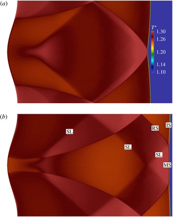
. The IS (respectively MS) section is located in the centre (respectively on the sides) of figure 11(d) (before collision), whereas its location appears switched in figure 12(b) (after collision). Accordingly, the IS is always located between approaching triple points and, vice versa, the MS is located between departing triple points. Notice that the displacement direction of the triple points can be inferred by looking at their distance of separation in subsequent snapshots: for instance, their separation decreases with time in figures 11(c) and 11(d) and increases in figures 12(a) and 12(b). An inversion is also observed between figures 10(c) and 11(b). The collision between the triple points occurs on the upper and lower horizontal boundaries between
 $t=46~{\rm\mu}\text{s}$
and
 $t=54~{\rm\mu}\text{s}$
; see figures 11(a) and 11(b). Before the collision of the two triple points, the reflected shocks intersect at a point (on the horizontal axis) moving toward the incident shock; see figures 11(c) and 11(d). Near the leading shock wave, the reflected shock is quasi-parallel to the slip line of the other triple point. When the two triple points collide on the leading shock, the point of intersection of the two reflected shocks reaches the leading shock, the reflected shocks and the slip lines are superimposed and cross each other and are almost parallel; see figure 12(a) or the two figures 11(a) and 11(b). At first sight, the triple points appear to cross each other without deformation. This is not quite the case, since the entrance angle between the trajectories of the triple points before collision is different from the exit angle after collision; see Fickett & Davis (Reference Fickett and Davis1979). This is also observed in the DNS and in the model equation discussed in the next section.
Contour maps of normalised temperature after reflection: IS, incident shock; MS, Mach stem; RS, reflected shock; SL, slip line. (a)
 $t=46~{\rm\mu}\text{s}$
, (b)
 $54~{\rm\mu}\text{s}$
, (c)
 $62~{\rm\mu}\text{s}$
, (d)
 $70~{\rm\mu}\text{s}$
.

Contour maps of normalized temperature after reflection: IS, incident shock; MS, Mach stem; RS, reflected shock; SL, slip line.
 $t=84~{\rm\mu}\text{s}$
(a),
 $96~{\rm\mu}\text{s}$
(b).

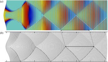
Trajectories of the triple points on the reflected shock: comparison between the DNS results (a), and the front evolution according to (4.1) (b) (the first tick on the horizontal axis denotes the location of the wall). (a) Shows a sequence of the actual shock profiles over time, coloured by the normalized temperature (minimum–maximum set at 1.21–1.30 to enhance the contrast between the MS and IS sections of the leading front; the dashed lines represents the trajectories of the lower triple point).

4.5. Comparison with a model equation
The spontaneous formation of triple points was theoretically analysed in previous works by Clavin (Reference Clavin2013) and Denet et al. (Reference Denet, Biamino, Lodato, Vervisch and Clavin2015). From these studies, a nonlinear wave equation describing the dynamics of the wrinkles of a shock interface was derived. This equation was obtained for strong shocks,
 $M_{1}\gg 1$
, in the Newtonian limit,
 $M_{1}^{2}({\it\gamma}-1)=O(1)$
, where the acoustic flow in the shocked gas is characterized by a lower intensity than the incompressible flow. Let the streamwise position of the perturbed shock be denoted as
 $x={\it\alpha}(y,t)$
, where
 $y$
is the spanwise coordinate, then the model equation written in the frame attached to the mean position of the leading shock reads
 $$\begin{eqnarray}\underbrace{\frac{\partial ^{2}{\it\alpha}}{\partial t^{2}}-a_{2}^{2}\frac{\partial ^{2}{\it\alpha}}{\partial y^{2}}}_{\text{wave equation}}+\underbrace{a_{1}M_{1}\frac{\partial }{\partial t}\left(\frac{\partial {\it\alpha}}{\partial y}\right)^{2}}_{\text{nonlinear term}}=0,\end{eqnarray}$$
where
 $a_{1}$
and
 $a_{2}$
are defined as the speed of sound on the supersonic and subsonic sides of the shock, respectively. Equation (4.1) is the combination of a wave equation, which accounts for the propagation of shock deformations along its surface at the speed
 $a_{2}$
, with a nonlinear term – proportional to
 $u_{1}=a_{1}M_{1}$
– which is responsible for the generation of cusps from smooth deformations of the shock front. Generally speaking, the linear modes are such that the intersection points of the acoustic waves with the leading shock propagate transversally along the shock front at the same velocity as the intersection points of the entropy–vorticity wave. In the asymptotic limit
 $M_{1}\gg 1$
,
 $M_{1}^{2}({\it\gamma}-1)=O(1)$
, the acoustic waves and the entropy–vorticity wave are, respectively, quasi-perpendicular and quasi-parallel to the shock front. Therefore, the transverse (vertical) propagation velocity of the disturbances on the front is
 $a_{2}$
, to the leading order. The conditions under investigation in this paper,
 $M_{1}\approx 1.43$
for the reflected shock and
 ${\it\gamma}=1.4$
, are far from the limit considered in the theoretical analysis,
 $M_{1}\gg 1$
. As a consequence the angle between the secondary shock waves (propagating in the normal direction nearly at the speed of sound
 $a_{2}$
in the shocked gas) and the leading shock is about 45°, which is very different from the nearly 90° predicted by the above analysis. Nevertheless, a tentative comparison between the model equation and the DNS can be undertaken, provided that
 $a_{2}$
in (4.1) is replaced by the observed vertical displacement velocity of the triple points,
 $|u_{T}|=310~\text{m}~\text{s}^{-1}$
, and the horizontal displacement velocity of the leading shock in the laboratory frame is introduced,
 $\mathscr{D}_{r}=325~\text{m}~\text{s}^{-1}$
(see § 3).
With such modifications, (4.1) is solved numerically with a sixth-order Padé scheme for a duration of
 $210~{\rm\mu}\text{s}$
. The initial condition
 ${\it\alpha}(y,0)$
is set using the shock profile extracted from the DNS at a time of
 $4~{\rm\mu}\text{s}$
after its reflection on the wall. The time evolution of the shock front obtained from (4.1) is depicted in figure 13(b), where subsequent profiles are shown every
 $2~{\rm\mu}\text{s}$
and horizontally translated according to the propagation velocity of the reflected shock,
 $\mathscr{D}_{r}$
. On figure 13(a), a sequence of snapshots of the actual shock profile over time is shown, coloured by the normalized temperature. Notice that the colour map has been set so as to enhance the contrast between the Mach stem and the incident shock sections of the leading shock. The trajectory of the bottom triple point is traced by a hand-drawn dashed line.
As can be seen, the main features of the shock dynamics and the formation and displacement of the triple points are qualitatively well reproduced. The nonlinear term in the model equation leads to the formation of cusps, corresponding to the triple points in the DNS, which propagate along the shock front. As previously pointed out by Denet et al. (Reference Denet, Biamino, Lodato, Vervisch and Clavin2015), an asymmetry in the trajectories of the cusps is observed before and after each collision. Although less pronounced, the same asymmetry is also visible in the DNS. After few collisions of the triple points, their trajectories become straight and the above-mentioned asymmetry is progressively lost. The curvature of the shock front decreases as well. In the early stages, after the cusps are generated on the profile, the model equation produces an excess in their vertical displacement velocity and their first collision happens earlier than in the DNS. This excess in the vertical velocity is clearly responsible for the mismatch in the longitudinal size of the cellular structures which, later on and after the initial transient, are about 12 % shorter than in the DNS (cf. the black arrow in figure 13).
Considering the mismatch between the limiting hypotheses in deriving (4.1) and the actual flow parameters adopted in the DNS, namely the limit of very large Mach numbers in the former compared to the value of 1.43 in the latter (which also includes viscous effects), a better quantitative agreement cannot be expected. It is not fully clear, at this stage, whether or not viscous effects have a significant influence in explaining the observed discrepancy between the model equation and the DNS. The comparison with the results from inviscid computations reported in § 4.2 seems to indicate that this is not the case. Future investigations are planned to approach the limit of large Mach numbers through DNS and, possibly, clarify this point.
5. Instantaneous flow fields
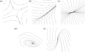
The complex flow field associated with the transverse waves propagating in the shocked gas is strongly unsteady, as shown in figures 8 and 15–22. The arrows along the streamlines in these figures indicate the direction of the flow in the fixed reference frame of the laboratory. To enhance clarity, critical points, as detailed in the following discussion, are labelled when needed in the relevant figures as: SD for saddle points, BL for bifurcation lines, ND for nodes, FC for foci and NF for node-focus points (cf. figure 14).
Critical points extracted from the shock wavy-wall DNS: (a) is a long-lived stagnation point, (b) is an accumulation line similar to the picture obtained in a section of a bifurcation line in three-dimensional flows, (c–e) are short-lived sinks or sources depending on the flow direction. They are respectively called stable and unstable critical points in the terminology used in the phase space of autonomous ordinary differential equations. (a) Saddle (SD), (b) bifurcation line (BL), (c) node (ND), (d) focus (FC), (e) node-focus (NF).

5.1. Transient critical points in two-dimensional compressible flows
In order to obtain precise information about the flow topology and its evolution in the shocked region, here the instantaneous streamline patterns are thoroughly examined at different instants in time. One of the most striking features is the existence of several types of critical points in the instantaneous streamline patterns of the two-dimensional and unsteady shocked flow within the compressed gas. For more details about the description of flow patterns using critical points, the reader is referred to the works of Perry & Chong (Reference Perry and Chong1987) and Chong et al. (Reference Chong, Perry and Cantwell1990) and references therein. In the absence of sources or sinks, the divergence of the velocity field is zero in two-dimensional incompressible flows. The only critical points that can then occur are foci (or vortices) and saddles (or stagnation points). The situation is different in unsteady two-dimensional compressible flows, in which a large variety of critical points can be observed, as is the case for three-dimensional incompressible flows. The unsteady term in the equation of mass conservation (time derivative of density) can introduce transient source or sink points in the form of nodes or node-foci. Examples of the diverse critical points of the flow, extracted from the present numerical simulation, are reported in figure 14.
It is worthwhile stressing, at this point, the importance of adopting a high-order numerical platform in the computation to deal with the broad range of velocity scales. The flow velocity of the shocked gas is typically of the order of
 $2{-}10~\text{m}~\text{s}^{-1}$
. These values are relatively small compared to the local speed of sound, about
 $450~\text{m}~\text{s}^{-1}$
, the transverse velocity of the triple points,
 $310~\text{m}~\text{s}^{-1}$
and the propagation velocity of the leading shock wave in the laboratory frame of reference,
 $325~\text{m}~\text{s}^{-1}$
. These high velocities introduce a short characteristic time for the evolution of the flow field, which is of the same order of magnitude as the transit time of acoustic waves, typically a few
 ${\rm\mu}\text{s}$
. This explains the compressible nature of the flow field in the shocked gases, despite the small velocities that characterize it. The small value of the flow velocity in the laboratory reference frame is related to the fact that, in the absence of wrinkles or multi-dimensional effects, the shocked gas of a planar shock – reflected from a planar wall with zero angle of incidence – is at rest.
5.2. The formation of the triple points
The formation of the triple points a brief time after the shock reflection follows a quite complicated scenario that can be analysed in terms of critical point flows. In the computation, a no-slip condition (zero velocity) is used at the wavy wall. Up to
 $14~{\rm\mu}\text{s}$
after reflection, the front of the leading shock is smoothly deformed; see figure 8(a,b). The flow field in the shocked gas presents saddle points at the crests of the sinusoidal wall (top and bottom of the figures) and at the troughs (central axis of the figures). These critical points are connected by an unsteady flow in the boundary layers, which flows, at early stages, from the crests to the troughs. This corresponds to the opposite horizontal components of the flow velocity at the trough and at the crest: the flow velocity at the trough is oriented from left to right, namely, toward the leading shock and in the same direction as the propagation of the shock, while the flow at the crest is oriented in the opposite direction, namely, toward the wall. The flow in the boundary layers is necessarily strongly unsteady, for the density and the pressure of the shocked gas are larger near the troughs than they are near the crests; accordingly, the reflected shock wave is stronger near the troughs and weaker near the crests. An abrupt transition then occurs between 14 and
 $18~{\rm\mu}\text{s}$
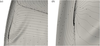
, when a critical point of the node-focus type suddenly appears near the wall on both sides of the horizontal axis of the troughs, as shown in figure 8(c,d). Enlarged views of this node-focus point are presented in figure 15. A sudden inversion of the flow is thus produced, alongside the trough, in the boundary layers. The connection with the flow coming from the crest is made through a new saddle point in the boundary layer, from which streamlines are issued along a line, almost perpendicular to the wall, toward the leading shock, as shown in figure 8(d). This line, toward which the flow trajectories are asymptotic, is in fact a bifurcation line (cf. figure 14). The intersection of this bifurcation line with the leading shock occurs just below a cusp that is beginning to appear on the shock front and from which a weak transverse shock is formed. The bifurcation line is then transformed into this transverse weak shock moving upwards attached to the cusp of the leading shock; see figure 8(e). Notice that a saddle point is also formed on the bifurcation line at about
 $t=20~{\rm\mu}\text{s}$
. This saddle point moves toward the leading shock wave, as shown in figure 8(e–g). It reaches the cusp at
 $t=30~{\rm\mu}\text{s}$
and forms the slip line which can be seen issuing from the triple point in figures 8(g) and 10(b). At the same time the flows in the boundary layers are completely reversed and are oriented from the troughs to the crests.
Close-up of the flow pattern above the trough at
 $t=18~{\rm\mu}\text{s}$
(figure 8
d): system of unstable node-focus/saddle/bifurcation line (a) and enlarged view of the node-focus only (b).

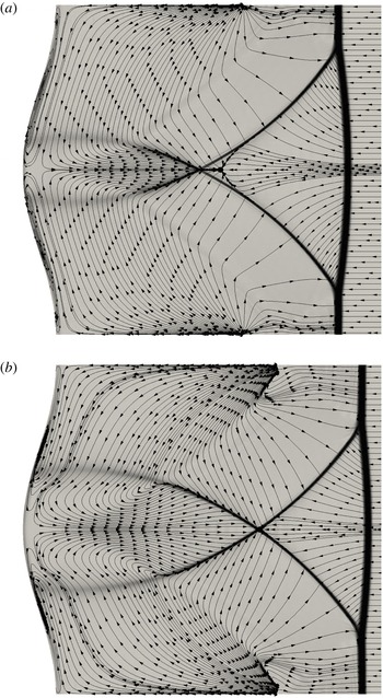
Time evolution of the flow streamlines and Schlieren image after reflection (SD, saddle point; BL, bifurcation line; ND, node; NF, node-focus; I, interaction point. (a)
 $t=34~{\rm\mu}\text{s}$
, (b)
 $38~{\rm\mu}\text{s}$
, (c)
 $42~{\rm\mu}\text{s}$
, (d)
 $46~{\rm\mu}\text{s}$
.

As a result of the formation of the two cusps on the leading shock, the front between them – namely, the Mach stem portion – that was initially straight, becomes slightly curved as the triple points move away from the centreline; see the sequential snapshots in figures 8(d–g) and 16(a–d).
5.3. Flow patterns resulting from the interaction between the transverse waves
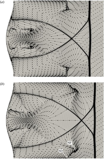
Time evolution of the flow streamlines and Schlieren image after reflection. (a)
 $t=50~{\rm\mu}\text{s}$
, (b)
 $54~{\rm\mu}\text{s}$
.

Time evolution of the flow streamlines and Schlieren image after reflection. (a)
 $t=58~{\rm\mu}\text{s}$
, (b)
 $62~{\rm\mu}\text{s}$
.

Time evolution of the flow streamlines and Schlieren image after reflection. (a)
 $t=66~{\rm\mu}\text{s}$
, (b)
 $70~{\rm\mu}\text{s}$
.

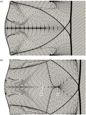
Time evolution of the flow streamlines and Schlieren image after reflection. (a)
 $t=74~{\rm\mu}\text{s}$
, (b)
 $84~{\rm\mu}\text{s}$
.

Time evolution of the flow streamlines and Schlieren image after reflection. (a)
 $t=90~{\rm\mu}\text{s}$
, (b)
 $96~{\rm\mu}\text{s}$
.

The flow patterns produced by the interaction between the transverse waves is strongly unsteady and the topology of the instantaneous streamlines is characterized by intermittent appearances of short-lived critical points. We will limit the following presentation to some basic features.
The first interaction between the transverse shocks occurs near the wall crest, at about
 $t=30~{\rm\mu}\text{s}$
; see figure 8(g). The point of intersection then propagates toward the leading shock on the horizontal lines that define the top and the bottom of figure 16. To the right of this point of intersection (cf. figure 16
b), the branches that connect with the triple points on the leading shock show a relatively marked discontinuity in the velocity field and the streamlines end at the front at an angle. This angle indicates that the velocity components normal to the front are discontinuous, as expected across a shock. As explained in § 3, these branches are sonic shock fronts (see, for instance, point A in table 2 and the relevant figure 7). The branches to the left of the above-mentioned point of intersection, which descend down to the wall, appear to have retained a bifurcation line topology.
As the strength of the transverse shocks increases, saddle points appear near the middle of these shocks. Stronger gradients of density are present on the right of these points, whereas weaker gradients characterize the tail on the left. These saddle points are clearly visible in figure 16(c). Before the first collision of the triple points on the leading shock, which occurs between
 $t=46~{\rm\mu}\text{s}$
and
 $t=50~{\rm\mu}\text{s}$
(see figures 16
d and 17
a), the interaction between the node-focus points near the wall and the slip lines that are visible in figure 11(a), leads to the formation of short-lived pairs of counter-rotating vortices. These are depicted in figure 16(d). At that time the flow is fully reversed at the external side of the thin boundary layers on the wavy wall. Moreover, stagnation (saddle) points are formed at two locations on the horizontal central axis, one close to the wall and the other near the leading shock. With regard to the latter, it appears that the main mechanism responsible for its appearance is the progressive decrease of horizontal momentum between
 $34~{\rm\mu}\text{s}$
and
 $46~{\rm\mu}\text{s}$
(see figure 16), to the point that the flow is reversed and a stagnation point is formed. Evidence of this decrease of momentum is the fact that the streamlines of the central flow field in the shocked gas are progressively opening out toward the leading shock. In fact, given a relatively unchanged curvature of the Mach stem (cf. figure 11
a) and the fixed value of the velocity upstream of the leading shock, it is easily shown that the gradual spreading of the streamlines is a consequence of the decrease of the horizontal component of velocity while preserving its tangential component across the leading shock.
A few
 ${\rm\mu}\text{s}$
later the above-mentioned counter-rotating vortices are swept by the tail of transverse shocks that approach the central line; see figure 17(a). As depicted in figures 17(b) and 18(a), these shocks begin to interact on the centreline and form a crossing point which propagates toward the leading shock. In front of the crossing point, a saddle is also visible, which is first transformed into a (sink) node and then swept away by the transverse shocks (see figure 18). At the same time the nodes that were formed on the horizontal lines at the top and bottom left of figure 16(c,d) are split into a system of node-foci separated by a saddle (cf. figures 18 and 19). This is due to the interaction with the slip lines visualized in figure 11(c). These foci will then merge and disappear as the transverse shocks get closer, but will seed a second rank of counter-rotating vortices above the wall crests, where the slip lines meet (the first rank is represented by the vortices induced by the central flow over the wall trough). These ranks of counter-rotating vortices are clearly visible in figure 21(a). Notice that a similar (but stronger) hierarchy of counter-rotating vortices can also be seen in the numerical simulation of detonations by Bourlioux & Majda (Reference Bourlioux and Majda1992) in the case of large heat release and low activation energy described therein.
Another intriguing feature is the simultaneous formation of a saddle and a node at the same point near the middle of the horizontal central axis at
 $t\approx 80~{\rm\mu}\text{s}$
. They are already separated in figure 20(b). The position of the saddle appears stationary whereas the node moves forwards. Later on, at
 $t\approx 90~{\rm\mu}\text{s}$
, the latter splits into a system of node-foci with a saddle in the middle (see figure 21), after having been crossed by the interacting slip lines that are depicted in figure 12(b). This mechanism appears similar to the one already observed over the wall crests, and will later determine the onset of a third rank of counter-rotating vortical structures on the centreline. These vortices are visible in figure 22(b). As can be evinced by looking at the different frames in figure 22, although the flow structure grows rapidly in complexity, the mechanism described above – the node splitting into a foci-saddle system – appears to be at the base of the formation of a hierarchy of counter-rotating vortex pairs, even far away from the wavy wall. These vortex pairs are formed by the above-mentioned mechanism at the crossing location of the slip lines left behind in the shocked gas by the leading reflected shock.
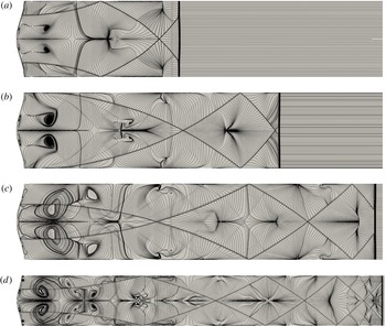
Time frames of the evolution of the flow streamlines and Schlieren image after reflection. (a)
 $t=120~{\rm\mu}\text{s}$
, (b)
 $200~{\rm\mu}\text{s}$
, (c)
 $280~{\rm\mu}\text{s}$
, (d)
 $440~{\rm\mu}\text{s}$
.

Also note that, due to the continuous interaction with the transverse shocks and the repeated inversion in flow direction, the boundary layers at the wall are eventually completely detached and destabilized, as can be seen in figures 5 and 22(d).
6. Discussion and conclusion
In the present study, the cellular structure created by the rebound of a planar (inert) shock from a wavy wall with a sinusoidal profile of small amplitude has been addressed with direct numerical simulation using a high-order spectral difference discretization of the Navier–Stokes equations in their fully compressible form, combined with a specific treatment to capture the shock with minimum perturbation and dissipation of the flow away from discontinuities.
The main properties of the shock reflection, as well as its propagation speed after rebound, the global flow topology featuring transverse propagating waves and the displacement speed of triple points travelling along the shock surface, have been compared to experimental observations to validate the numerical procedure.
Despite the fact that the wall geometry had been purposely designed to prevent the transition from regular reflection to Mach reflection during the interaction with the incident shock, both the experimental and numerical results have shown the spontaneous formation of triple points and Mach stems on the shock front a few moments after its reflection from the wall. As a direct consequence of the formation of triple points – featuring typical systems with a Mach stem, an incident shock, a reflected shock and a slip line – and their subsequent mutual interactions, complex flow patterns have been observed in the shocked gases. Such patterns are the result of subsequent and repeated interactions between transverse fronts and slip lines, which are originated at the triple points on the reflected shock.
The comparison between the results of computations using no-slip and free-slip wall boundary conditions reveals that the flow field in the shocked gases is mostly due to the dynamics of the reflected shock and the triple points, the impact of the wall boundary layer being negligible away from it. Even though it is not easy to clearly separate the causes from the effects, the complex flow field in the shocked gas looks mainly driven by the dynamics of the triple point on the shock front. The feedback of the nonlinear flow patterns on the dynamics of the shock is limited to the near field responsible for the Mach-stem formation. Once they are formed, the dynamics of the triple points, sufficiently far from the wavy wall, is no longer affected by the complex flow in the shocked gas, as shown by the regular trajectories of triple points in figure 13.
This leads the authors to think that the nonlinear dynamics of the wrinkled shock wave could be described in the general case by a local equation, as is the case in the asymptotic limit
 $M_{1}\gg 1$
,
 $M_{1}^{2}({\it\gamma}-1)=O(1)$
investigated by Clavin (Reference Clavin2013). The numerical solution of an extension of (4.1), using for initial condition the smoothly wrinkled shock front obtained by the DNS just after reflection, shows a nonlinear dynamics of the shock front quite similar to that observed in the DNS and the companion experiment.
Striking similarities have been clearly highlighted with the cellular structure of weakly unstable detonations. The observed similarities suggest – and further confirm (Clavin & Denet Reference Clavin and Denet2002; Clavin Reference Clavin2013) – that the nonlinear mechanisms responsible for the formation of the triple points and Mach stems on a weakly unstable detonation are inherent in the dynamics of the leading (inert) shock front. Near to the multi-dimensional instability threshold, the role of the combustion is thus limited to the linear instability. This conclusion concerns weakly unstable detonations only. The case of strongly unstable detonations mentioned in the second paragraph of the Introduction is much more complex. However, the present analysis shows that the cellular pattern on the leading shock is not affected by the complex flow in the shocked gas. To what extent this could also be true for strongly unstable detonations remains an open question that deserves further studies.
Another result of our analysis is that the gas viscosity has a negligible effect on the observed flow patterns and cannot be responsible for the flatness of the shock front. The relaxation to a flat front, then, could result from the nonlinear dynamics of the triple points in the periodic cellular pattern. This is suggested by the comparison with the solution to the model (4.1) in figure 13, which also shows a relaxation toward a quasi-flat front in the absence of any linear dissipative term. In figure 1, the direct numerical simulation also shows that the proximity of the end wall, just after the reflection, increases the initial relaxation rate to a flat front, as soon as the triple points are formed. The linear effects of a strong viscosity, namely, higher than that of a gas, as in liquids or melted metals, is an open question. However, according to our nonlinear analysis in gases, which shows that the effect of viscosity is dominated by the relevant nonlinear terms, it is doubtful – and remains to be confirmed – that the linear viscous damping, reported for instance by Miller & Ahrens (Reference Miller and Ahrens1991), could dominate the nonlinear dynamics.
From the high-order simulations and the relevant detailed description of the flow in the shocked gases, the exact nature of the transverse waves appearing during the interaction between the wavy wall and the planar shock has been elucidated. The results can be summarized as follows. The reverse jets formed by the flow impacting on the troughs of the wavy wall are confined by bifurcation lines. The transverse waves emerge from the progressive transformation of these bifurcation lines into sonic propagating discontinuities, or transverse reflected shocks, attached to the triple points, which in turn travel back and forth along the shock surface. The transition between the topology of the bifurcation lines and the sonic fronts appears to be characterized by the presence of a saddle point. Unstable node-foci also develop at the tails of the slip lines which emanate from the triple points. The interaction between the slip lines and the reflected branches of the transverse shocks leads to the formation of counter-rotating vortices. The mutual interaction of the transverse shocks, in the form of collisions between them, leads to the formation of stagnation points and sources. These source points, in particular, move in the shocked gases, following the reflected shock front until they reach regions of strong vorticity generated by contiguous pairs of slip lines. The consequent interaction appears to be the driving mechanism responsible for the onset of counter-rotating vortex pairs.
Acknowledgements
The use of the SD solver originally developed by Antony Jameson’s group at Stanford University, and financial support of the first Author by CNRS under the INSA Turbulence and Simulation Chair are gratefully acknowledged. This work was granted access to the HPC resources of IDRIS-CNRS under the allocation 2015-2b152 made by GENCI (Grand Equipement National de Calcul Intensif). The Haute Normandie Computing center CRIHAN is also acknowledged. We would also like to thank L. Houas, G. Jourdan and L. Biamino from IUSTI (Marseilles) for providing us with the experimental data.
Appendix A
The two-dimensional Navier–Stokes equations for gas dynamics are solved using the high-order spectral difference method for unstructured spatial discretization. The formulation of the equations on quadrilateral grids is similar to the one described by Sun, Wang & Liu (Reference Sun, Wang and Liu2007), which is summarized below for completeness. The unsteady compressible Navier–Stokes equations in conservative form are written as
 $$\begin{eqnarray}\frac{\partial \boldsymbol{U}}{\partial t}+\frac{\partial \boldsymbol{F}^{i}}{\partial x_{i}}=\mathbf{0}\quad (i=1,2),\end{eqnarray}$$
where
 $t$
represents the time,
 $\boldsymbol{x}=(x_{1},x_{2})$
the position vector,
 $\boldsymbol{U}=\left(\begin{array}{@{}cccc@{}}{\it\rho} & {\it\rho}u_{1} & {\it\rho}u_{2} & {\it\rho}e\end{array}\right)^{\text{T}}$
is the vector of conservative variables, and
 $\boldsymbol{F}^{i}=\boldsymbol{F}_{conv}^{i}+\boldsymbol{F}_{visc}^{i}$
account for the convective and viscous fluxes, respectively,
 $$\begin{eqnarray}\boldsymbol{F}_{conv}^{i}=\left(\begin{array}{@{}c@{}}{\it\rho}u_{i}\\ {\it\rho}u_{1}u_{i}+{\it\delta}_{1i}p\\ {\it\rho}u_{2}u_{i}+{\it\delta}_{2i}p\\ ({\it\rho}e+p)u_{i}\end{array}\right)\quad \text{and}\quad \boldsymbol{F}_{visc}^{i}=\left(\begin{array}{@{}c@{}}0\\ -2{\it\mu}\unicode[STIX]{x1D608}_{1i}\\ -2{\it\mu}\unicode[STIX]{x1D608}_{2i}\\ -2{\it\mu}u_{j}\unicode[STIX]{x1D608}_{ij}-{\it\lambda}\displaystyle \frac{\partial T}{\partial x_{i}}\end{array}\right).\end{eqnarray}$$
In the above equations,
 ${\it\rho}$
is the fluid density,
 $\boldsymbol{u}=(u_{1},u_{2})$
is the velocity vector,
 ${\it\delta}_{ij}$
is the Kronecker delta,
 $p$
is the pressure,
 ${\it\mu}$
is the dynamic viscosity,
 ${\it\lambda}={\it\mu}c_{p}/Pr$
is the thermal conductivity (computed from the Prandtl number
 $Pr$
), and
 $e$
is the total energy (internal
 $+$
kinetic). This last is related to the pressure by assuming the validity of the ideal gas law,
 $$\begin{eqnarray}\frac{p}{{\it\rho}}=({\it\gamma}-1)c_{v}T,\quad {\it\rho}e=\frac{p}{{\it\gamma}-1}+\frac{1}{2}{\it\rho}u_{i}u_{i},\end{eqnarray}$$
where
 ${\it\gamma}=c_{p}/c_{v}$
is the ratio between specific heat capacities at constant pressure and constant volume. The tensor
 $\unicode[STIX]{x1D608}_{ij}$
in (A 2a,b
) is the deviator of the deformation tensor, namely,
 $$\begin{eqnarray}\unicode[STIX]{x1D608}_{ij}=\frac{1}{2}\left(\frac{\partial u_{i}}{\partial x_{j}}+\frac{\partial u_{j}}{\partial x_{i}}\right)-\frac{1}{3}{\it\delta}_{ij}\frac{\partial u_{k}}{\partial x_{k}}.\end{eqnarray}$$
To achieve an efficient implementation, each element in the physical domain is transformed to a standard square element described by local coordinates
 ${\bf\xi}=({\it\xi}_{1},{\it\xi}_{2})$
, with
 ${\bf\xi}\in [-1:1]^{2}$
. The governing equations in the physical domain are then transferred into the computational domain, and they take the form
 $$\begin{eqnarray}\frac{\partial \boldsymbol{{\mathcal{U}}}}{\partial t}+\frac{\partial \boldsymbol{{\mathcal{F}}}^{i}}{\partial {\it\xi}_{i}}=\mathbf{0},\end{eqnarray}$$
 $$\begin{eqnarray}\boldsymbol{{\mathcal{U}}}=\text{det}(\unicode[STIX]{x1D645})\boldsymbol{U},\quad \boldsymbol{{\mathcal{F}}}=\text{adj}(\unicode[STIX]{x1D645})\boldsymbol{\cdot }\boldsymbol{F},\end{eqnarray}$$
where
 $\text{det}(\unicode[STIX]{x1D645})$
and
 $\text{adj}(\unicode[STIX]{x1D645})$
represent the determinant and the adjoint of the Jacobian matrix
 $\unicode[STIX]{x1D611}_{ij}=\partial x_{i}/\partial {\it\xi}_{j}$
, respectively.
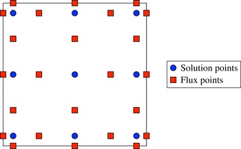
Schematic representation of the two-dimensional distribution of solution and flux points within the SD element for
 $n=3$
.

Within each standard element, two sets of points are defined, namely, the solution points and the flux points, as schematically illustrated in figure 23. In order to construct a degree
 $n-1$
polynomial for each coordinate direction, solutions at
 $n$
points are required. These
 $n$
points in one dimension are chosen to be the Gauss–Legendre quadrature points, whereas the flux points are selected to be the Gauss–Legendre quadrature points of order
 $n-1$
plus the two end points at
 ${\it\xi}=-1$
and
 ${\it\xi}=1$
, respectively. Accordingly, the
 $n$
solution points are obtained as the roots of the equation
 $$\begin{eqnarray}P_{n}({\it\xi})=\frac{2n-1}{n}{\it\xi}P_{n-1}({\it\xi})-\frac{n-1}{n}P_{n-2}({\it\xi})=0,\end{eqnarray}$$
where
 $P_{n}({\it\xi})$
is the Legendre polynomial of order
 $n$
,
 $P_{-1}({\it\xi})=0$
and
 $P_{0}({\it\xi})=1$
and
 ${\it\xi}$
is either
 ${\it\xi}_{1}$
or
 ${\it\xi}_{2}$
. This particular combination of solution and flux points, in particular, can be proved to be linearly stable for all orders of accuracy and is optimal in reducing aliasing errors and providing good conditioning for the nonlinear case (Jameson Reference Jameson2010; Jameson, Vincent & Castonguay Reference Jameson, Vincent and Castonguay2012). Using the
 $n$
solution points and the
 $n+1$
flux points, polynomials of degree
 $n-1$
and
 $n$
, respectively, can be built using Lagrange bases defined as
 $$\begin{eqnarray}h_{i}({\it\xi})=\mathop{\prod }_{\substack{ s=1 \\ s\neq i}}^{n}\left(\frac{{\it\xi}-{\it\xi}_{s}}{{\it\xi}_{i}-{\it\xi}_{s}}\right)\quad \text{and}\quad l_{i+1/2}({\it\xi})=\mathop{\prod }_{\substack{ s=0 \\ s\neq i}}^{n}\left(\frac{{\it\xi}-{\it\xi}_{s+1/2}}{{\it\xi}_{i+1/2}-{\it\xi}_{s+1/2}}\right).\end{eqnarray}$$
The reconstructed solution for the conserved variables in the standard element is then obtained as the tensor product of the two one-dimensional polynomials,
 $$\begin{eqnarray}\boldsymbol{U}({\bf\xi})=\mathop{\sum }_{j=1}^{n}\mathop{\sum }_{i=1}^{n}\frac{\boldsymbol{{\mathcal{U}}}_{i,j}}{\text{det}(\unicode[STIX]{x1D645})_{i,j}}h_{i}({\it\xi}_{1})h_{j}({\it\xi}_{2}),\end{eqnarray}$$
where
 $i$
and
 $j$
are the indices of the solution points within each standard element. Similarly, the reconstructed flux polynomials take the following form:
 $$\begin{eqnarray}\displaystyle & \displaystyle \boldsymbol{{\mathcal{F}}}^{1}({\bf\xi})=\mathop{\sum }_{j=1}^{n}\mathop{\sum }_{i=0}^{n}\boldsymbol{{\mathcal{F}}}_{i+1/2,j}^{1}\,l_{i+1/2}({\it\xi}_{1})\,h_{j}({\it\xi}_{2}), & \displaystyle\end{eqnarray}$$
 $$\begin{eqnarray}\displaystyle & \displaystyle \boldsymbol{{\mathcal{F}}}^{2}({\bf\xi})=\mathop{\sum }_{i=1}^{n}\mathop{\sum }_{j=0}^{n}\boldsymbol{{\mathcal{F}}}_{i,j+1/2}^{2}\,l_{j+1/2}({\it\xi}_{2})\,h_{i}({\it\xi}_{1}). & \displaystyle\end{eqnarray}$$
The reconstructed fluxes are only element-wise continuous, but discontinuous across cell interfaces. With regard to the convective flux contribution, a Riemann solver is employed to compute a common flux at the cell interfaces to ensure conservation and stability. In the current implementation, the Roe solver with entropy fix (Roe Reference Roe1981; Harten Reference Harten1983) is used. The left and right states here represent the solution on both sides of the shared edge flux point. Hence, along the
 ${\it\xi}_{1}$
direction, the reconstructed fluxes in (A 10) and (A 11) are made continuous by replacing the element interface fluxes
 $\boldsymbol{{\mathcal{F}}}_{1/2,j}^{1}$
and
 $\boldsymbol{{\mathcal{F}}}_{n+1/2,j}^{1}$
with the numerical interface fluxes
 $\boldsymbol{{\mathcal{F}}}_{L,j}^{1}$
and
 $\boldsymbol{{\mathcal{F}}}_{R,j}^{1}$
at the left and right element interfaces, respectively (similarly for the
 ${\it\xi}_{2}$
direction). The (continuous of order
 $n$
) flux polynomial functions can be written as
 $$\begin{eqnarray}\displaystyle & \displaystyle \boldsymbol{{\mathcal{F}}}^{1}({\bf\xi})=\mathop{\sum }_{j=1}^{n}\left[\mathop{\sum }_{i=1}^{n-1}\boldsymbol{{\mathcal{F}}}_{i+1/2,j}^{1}l_{i+1/2}({\it\xi}_{1})+\boldsymbol{{\mathcal{F}}}_{L,j}^{1}l_{1/2}({\it\xi}_{1})+\boldsymbol{{\mathcal{F}}}_{R,j}^{1}l_{n+1/2}({\it\xi}_{1})\right]h_{j}({\it\xi}_{2}), & \displaystyle\end{eqnarray}$$
 $$\begin{eqnarray}\displaystyle & \displaystyle \boldsymbol{{\mathcal{F}}}^{2}({\bf\xi})=\mathop{\sum }_{i=1}^{n}\left[\mathop{\sum }_{j=1}^{n-1}\boldsymbol{{\mathcal{F}}}_{i,j+1/2}^{2}l_{j+1/2}({\it\xi}_{2})+\boldsymbol{{\mathcal{F}}}_{i,L}^{2}l_{1/2}({\it\xi}_{2})+\boldsymbol{{\mathcal{F}}}_{i,R}^{2}l_{n+1/2}({\it\xi}_{2})\right]h_{i}({\it\xi}_{1}). & \displaystyle\end{eqnarray}$$
The continuous viscous flux polynomial functions are obtained, with similar relations to (A 12) and (A 13), after computing common interface viscous fluxes as a function of the average interface solution and solution gradient (Sun et al. Reference Sun, Wang and Liu2007).
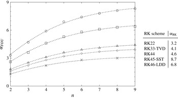
Explicit time integration is performed via the Runge–Kutta methodology. Several different types of Runge–Kutta schemes are available in the present numerical solver, such as the standard second- (RK22) and fourth-order (RK44) schemes with two and four stages, respectively. The third-order three-stage total variation diminishing (RK33-TVD), the fourth-order five-stage strong stability preserving (RK45-SST) and the low-storage fourth-order six-stage low-dispersion/dissipation (RK46-LDD) Runge–Kutta schemes are also implemented (see Gottlieb & Shu Reference Gottlieb and Shu1998; Spiteri & Ruuth Reference Spiteri and Ruuth2002; Bogey & Bailly Reference Bogey and Bailly2004, respectively).
The stability in time is ensured by setting the maximum time step to satisfy the Courant–Friedrichs–Lewy (CFL) and Fourier (FOU) conditions for the convective and diffusive fluxes, respectively. The maximum time steps for the CFL and FOU conditions is computed as the maximum value within the computational domain of
 $1/({\rm\Delta}t_{CFL}^{-1}+{\rm\Delta}t_{FOU}^{-1})$
, and
 ${\rm\Delta}t_{CFL}$
and
 ${\rm\Delta}t_{FOU}$
are locally defined as
 $$\begin{eqnarray}{\rm\Delta}t_{CFL}={\it\alpha}_{CFL}\frac{{\it\xi}_{s1}h}{{\it\lambda}}\quad \text{and}\quad {\rm\Delta}t_{FOU}={\it\alpha}_{FOU}\frac{({\it\xi}_{f2}h)^{2}}{2D{\it\nu}_{tot}},\end{eqnarray}$$
where
 $h$
is the element size,
 ${\it\xi}_{s1}h$
and
 ${\it\xi}_{f2}h$
represent the smallest distance of solution and flux points, respectively, to the element interface,
 ${\it\lambda}=\sqrt{u_{i}u_{i}}+a$
is the spectral radius of the convective flux Jacobian,
 $D$
is the dimension of the problem and
 ${\it\nu}_{tot}$
the total kinematic viscosity, which includes the molecular viscosity and the artificial viscosity from the shock capturing method (cf. appendix B). Notice that the values of
 ${\it\xi}_{s1}$
for the convective time step and
 ${\it\xi}_{f2}$
for the diffusive time step have been empirically selected to obtain an order-independent maximum time step in the case that a forward Euler time integration is used.
The coefficients
 ${\it\alpha}_{CFL}$
and
 ${\it\alpha}_{FOU}$
are introduced to adjust the limit of stability depending on the particular time integration scheme adopted. The former coefficient, in particular, is set to 1 for all the above-mentioned Runge–Kutta schemes but the RK45-SST, which allows a value of
 ${\it\alpha}_{CFL}=1.51$
(see Spiteri & Ruuth Reference Spiteri and Ruuth2002).
With regard to
 ${\it\alpha}_{FOU}$
, this coefficient is in general dependent on the order of the computation, the time integration scheme and the discretization scheme for the interface viscous fluxes. Empirical tests of pure diffusion of an initial Dirac profile, conducted using the present viscous flux by Sun et al. (Reference Sun, Wang and Liu2007), have highlighted a rather peculiar functional dependence between
 ${\it\alpha}_{FOU}$
and the order of the computation
 $n$
, namely,
 $$\begin{eqnarray}{\it\alpha}_{FOU}={\it\alpha}_{RK}\tanh (0.2\,n),\end{eqnarray}$$
where the values of
 ${\it\alpha}_{RK}$
for each Runge–Kutta scheme are determined by least-square fit of (A 15). The empirically determined limiting values of
 ${\it\alpha}_{FOU}$
, the fits from (A 15) and the relevant values of
 ${\it\alpha}_{RK}$
are reported in figure 24. Given the clear superiority of the RK45-SST in terms of maximum allowable time step, this scheme has been used to perform the DNS of the shock wavy-wall interaction presented in this study.
Limiting values of
 ${\it\alpha}_{FOU}$
as a function of the order
 $n$
(left) and values of the fit coefficients
 ${\it\alpha}_{RK}$
(right):
 $\times$
, RK22; ♢, RK33-TVD; ▵, RK44; ○, RK45-SST; ▫, RK46-LDD; - - - - - -, best fit using (A 15).

Appendix B
In general, high-order methods are susceptible to generating overshoots and undershoots in the neighbourhood of discontinuities. These spurious oscillations (frequently referred to as Gibbs phenomena) can be damped using artificial viscosity. However, if too much viscosity is added, then the quality of the solution may be detrimentally affected, even far from the shock. Thus, it is necessary to introduce artificial viscosity in a localized manner. In the best circumstances, the effects of artificial viscosity should be localized to a small part of each cell through which the shock passes.
In the present study, the method which is adopted is the one proposed by Persson & Peraire (Reference Persson and Peraire2006). This approach, which was originally developed for the discontinuous Galerkin (DG) scheme, combines a highly selective spectral sensor, based on the modal decomposition via orthogonal polynomials, with a consistently discretized artificial viscosity. The method smooths out the discontinuities in the solution to a width that is appropriately resolved by the mesh and the polynomial approximations. Hence, subcell resolution for high-order discretizations can be achieved. Moreover, if
 $p=n-1$
is the polynomial order of the solution, the amount of artificial viscosity is set to scale as
 $1/p$
and, for high-order polynomials, shock profiles which are much thinner than the element size can be obtained. The method is briefly summarized below.
The solved equation set, namely (A 1), is augmented with a Laplacian diffusion term,
 $$\begin{eqnarray}\frac{\partial \boldsymbol{U}}{\partial t}+\frac{\partial \boldsymbol{F}^{i}}{\partial x_{i}}=\frac{\partial }{\partial x_{i}}\left({\it\varepsilon}\frac{\partial \boldsymbol{U}}{\partial x_{i}}\right),\end{eqnarray}$$
where
 ${\it\varepsilon}$
represents the added artificial viscosity to be introduced in regions where the flow is under-resolved, such as across shocks and contact discontinuities. In order to sense these regions accurately, the level of smoothness of a selected variable
 ${\it\psi}$
, hereafter referred to as the sensor variable, is determined by checking the rate of decay of the expansion coefficients, or modal coefficients, of the solution in an orthogonal basis. In the present case, normalized orthogonal Legendre polynomials are adopted and the sensor variable is written as
 $$\begin{eqnarray}{\it\psi}({\it\xi})=\mathop{\sum }_{i=1}^{n}\hat{{\it\psi}}_{i}P_{i-1}^{\ast }({\it\xi}),\end{eqnarray}$$
where
 $P_{i}^{\ast }({\it\xi})$
is the normalised Legendre polynomial of degree
 $i$
, namely,
 $$\begin{eqnarray}P_{i}^{\ast }({\it\xi})=P_{i}({\it\xi})\sqrt{\frac{2\text{i}+1}{2}}\quad \Rightarrow \quad \int _{-1}^{1}P_{i}^{\ast }({\it\xi})P_{j}^{\ast }({\it\xi})\,\text{d}{\it\xi}={\it\delta}_{ij},\end{eqnarray}$$
and
 $\hat{{\it\psi}}_{i}$
are the modes of the sensor variable, which can be obtained from its nodal values through a simple matrix multiplication with the inverse Vandermonde matrix constructed using the selected polynomial basis (Hesthaven & Warburton Reference Hesthaven and Warburton2008).
After introducing the truncated expansion
 $$\begin{eqnarray}\overline{{\it\psi}}({\it\xi})=\mathop{\sum }_{i=1}^{n-1}\hat{{\it\psi}}_{i}P_{i-1}^{\ast }({\it\xi}),\end{eqnarray}$$
a resolution indicator (Persson & Peraire Reference Persson and Peraire2006; Persson Reference Persson2013), or sensor, inside each element is defined as
 $$\begin{eqnarray}s_{e}=\log _{10}\left[\frac{({\it\psi}-\overline{{\it\psi}},{\it\psi}-\overline{{\it\psi}})_{e}}{({\it\psi},{\it\psi})_{e}}\right],\end{eqnarray}$$
where
 $(\cdot \,,\cdot )_{e}$
is the standard inner product in the element. From (B 2) and (B 4), the orthonormality of the Legendre polynomial basis (cf. (B 3)), in particular, leads to the following simple expressions for the inner products in (B 5):
 $$\begin{eqnarray}({\it\psi}-\overline{{\it\psi}},{\it\psi}-\overline{{\it\psi}})_{e}=\!\int _{-1}^{1}\hat{{\it\psi}}_{n}^{2}P_{n-1}^{\ast }({\it\xi})P_{n-1}^{\ast }({\it\xi})\,\text{d}{\it\xi}=\hat{{\it\psi}}_{n}^{2},\end{eqnarray}$$
 $$\begin{eqnarray}\displaystyle ({\it\psi},{\it\psi})_{e}\! & = & \displaystyle \!\int _{-1}^{1}\mathop{\sum }_{i=1}^{n}\mathop{\sum }_{j=1}^{n}\hat{{\it\psi}}_{i}\hat{{\it\psi}}_{j}P_{i-1}^{\ast }({\it\xi})P_{j-1}^{\ast }({\it\xi})\,\text{d}{\it\xi}\end{eqnarray}$$
 $$\begin{eqnarray}\displaystyle \! & = & \displaystyle \!\mathop{\sum }_{i=1}^{n}\mathop{\sum }_{j=1}^{n}\hat{{\it\psi}}_{i}\hat{{\it\psi}}_{j}\int _{-1}^{1}P_{i-1}^{\ast }({\it\xi})P_{j-1}^{\ast }({\it\xi})\,\text{d}{\it\xi}=\mathop{\sum }_{i=1}^{n}\mathop{\sum }_{j=1}^{n}{\it\delta}_{ij}\hat{{\it\psi}}_{i}\hat{{\it\psi}}_{j}=\mathop{\sum }_{i=1}^{n}\hat{{\it\psi}}_{i}^{2}.\end{eqnarray}$$
Hence, the artificial viscosity is evaluated as
 $$\begin{eqnarray}{\it\varepsilon}_{e}=\left\{\begin{array}{@{}ll@{}}\displaystyle 0\quad & \displaystyle \text{for }s_{e}<s_{0}-{\it\kappa},\\ \displaystyle \frac{{\it\varepsilon}_{0}}{2}\left[1+\sin \frac{{\rm\pi}(s_{e}-s_{0})}{2{\it\kappa}}\right]\quad & \displaystyle \text{for }s_{0}-{\it\kappa}\leqslant s_{e}\leqslant s_{0}+{\it\kappa},\\ \displaystyle {\it\varepsilon}_{0}\quad & \displaystyle \text{for }s_{e}>s_{0}+{\it\kappa},\end{array}\right.\end{eqnarray}$$
where
 ${\it\varepsilon}_{0}$
,
 $s_{0}$
and
 ${\it\kappa}$
are additional parameters to be chosen empirically. In the present implementation,
 ${\it\varepsilon}_{0}$
is computed from the spectral radius of the flux Jacobian and the element size
 $h$
as
 $$\begin{eqnarray}{\it\varepsilon}_{0}={\it\lambda}_{max}h/(n-1),\end{eqnarray}$$
where
 ${\it\lambda}_{max}=\max (\sqrt{u_{i}u_{i}}+a)$
is the maximum wave speed in the whole domain and
 $a$
is the speed of sound (Barter & Darmofal Reference Barter and Darmofal2010).
Regarding the threshold
 $s_{0}$
and sensor tolerance
 ${\it\kappa}$
, these are computed via an auto-calibration algorithm, which, through a manufactured solution, is able to determine the optimal values for the shock-sensor parameters for an arbitrarily selected value of the order
 $n$
. In particular,
 $s_{0}$
is computed from the value of the sensor when a relatively sharp hyperbolic tangent profile is assumed for the solution. The relevant nodal values take the form
 $$\begin{eqnarray}{\it\psi}_{m.f.}({\it\xi}_{i})=\frac{1}{2}\left[1+\tanh \left(\frac{\text{tr}(i-1-n/2)+1/2}{(n-1)/5}\right)\right]\quad (i=1,\ldots ,n),\end{eqnarray}$$
where
 $\text{tr}(\cdot )$
represents truncation to the lower integer and is used to prevent the manufactured signal from being perfectly centred in the element of odd order
 $n$
, which is particularly undesirable for low orders (for
 $n=3$
, for example, this would make the manufactured signal linear and cause the threshold
 $s_{0}$
to be too low and the sensor to trigger artificial viscosity in smooth regions of the flow). If
 $s_{m.f.}$
is the value of the sensor for the manufactured solution, computed from (B 5), then
 $$\begin{eqnarray}s_{0}=s_{m.f.}-3\quad \text{and}\quad {\it\kappa}=1.\end{eqnarray}$$
Although the described calibration algorithm still involves some level of empiricism in the determination of the artificial viscosity parameters – namely, the correction to
 $s_{m.f.}$
in (B 12a,b
) and the value of
 ${\it\kappa}$
itself – the resulting values were found to work well in a variety of different test cases over a wide range of orders
 $n$
. A particularly desirable feature of this strategy effectively appears to be the removal of the order-dependence of the optimal parameters.
Also note that the element-wise viscosities from (B 9) are made
 $\mathscr{C}^{0}$
continuous as suggested by Persson (Reference Persson2013) by means of bilinear interpolation of the common values of
 ${\it\varepsilon}$
evaluated at the element interfaces.
Appendix C
Denoting by the subscript 1 and 2 the initial conditions and the conditions in the shocked gas respectively, the Rankine–Hugoniot relations for a planar shock wave propagating with a Mach number
 $M_{1}$
in an initial gas at rest take the form
 $$\begin{eqnarray}\displaystyle & \displaystyle \frac{p_{2}}{p_{1}}=\frac{2{\it\gamma}M_{1}^{2}-({\it\gamma}-1)}{{\it\gamma}+1}, & \displaystyle\end{eqnarray}$$
 $$\begin{eqnarray}\displaystyle & \displaystyle \frac{{\it\rho}_{2}}{{\it\rho}_{1}}=\frac{u_{1}^{s}}{u_{2}^{s}}=\frac{({\it\gamma}+1)M_{1}^{2}}{({\it\gamma}-1)M_{1}^{2}+2}, & \displaystyle\end{eqnarray}$$
 $$\begin{eqnarray}\displaystyle & \displaystyle M_{2}^{2}=\frac{({\it\gamma}-1)M_{1}^{2}+2}{2{\it\gamma}M_{1}^{2}-({\it\gamma}-1)}, & \displaystyle\end{eqnarray}$$
where
 $u_{1}^{s}$
and
 $u_{2}^{s}$
denote the normal flow velocities relative to the shock of the initial gas and the shocked gas, respectively, and
 $M_{1}=u_{1}^{s}/a_{1}$
with
 $a_{1}=\sqrt{{\it\gamma}p_{1}/{\it\rho}_{1}}$
.