1. Introduction
There has been a surge of interest in pore-scale modelling of reactive transport, with an increasing emphasis on coupling molecular scale processes to the evolution of porosity and mineral composition (Kang et al. Reference Kang, Tsimpanogiannis, Zhang and Lichtner2005; Lichtner & Kang Reference Lichtner and Kang2007; Li, Steefel & Yang Reference Li, Steefel and Yang2008; Mbogoro et al. Reference Mbogoro, Snowden, Edwards, Peruffo and Unwin2011; Molins et al. Reference Molins, Trebotich, Steefel and Shen2012, Reference Molins, Trebotich, Yang, Ajo-Franklin, Ligocki, Shen and Steefel2014; Chen et al. Reference Chen, Kang, Tang, Robinson, He and Tao2015; De Baere et al. Reference De Baere, Molins, Mayer and François2016; Pereira Nunes, Blunt & Bijeljic Reference Pereira Nunes, Blunt and Bijeljic2016; Starchenko, Marra & Ladd Reference Starchenko, Marra and Ladd2016; Soulaine et al. Reference Soulaine, Roman, Kovscek and Tchelepi2017; Molins et al. Reference Molins, Trebotich, Arora, Steefel and Deng2019; Oliveira, Blunt & Bijeljic Reference Oliveira, Blunt and Bijeljic2019; Dutka et al. Reference Dutka, Starchenko, Osselin, Magni, Szymczak and Ladd2020). Applications include subsurface hydrology, fossil-fuel extraction, environmental monitoring and  $\textrm {CO}_2$ sequestration. Recent experiments (Soulaine et al. Reference Soulaine, Roman, Kovscek and Tchelepi2017; Dutka et al. Reference Dutka, Starchenko, Osselin, Magni, Szymczak and Ladd2020) have shown that a soluble cylinder confined within a Hele-Shaw cell takes up a variety of shapes as it dissolves, which resemble one half of a lemniscate (or figure-of-eight). The evolving shapes have been used to validate numerical methods for simulating reactive transport at the pore scale (Soulaine et al. Reference Soulaine, Roman, Kovscek and Tchelepi2017; Molins et al. Reference Molins, Trebotich, Arora, Steefel and Deng2019; Dutka et al. Reference Dutka, Starchenko, Osselin, Magni, Szymczak and Ladd2020).
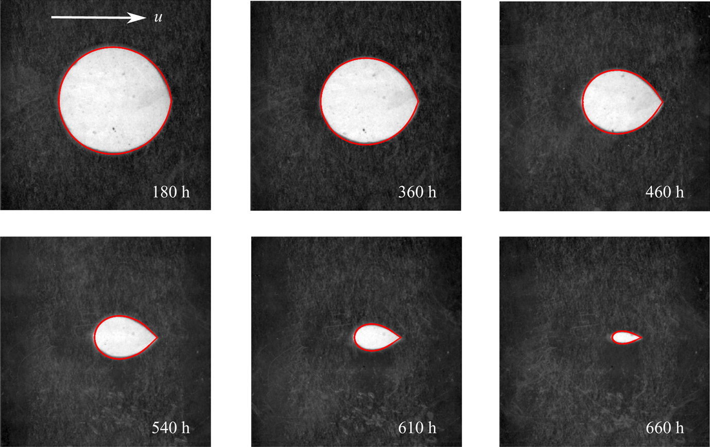
We recently noticed that shapes observed in these microfluidic experiments can be remarkably well described by a simple two-dimensional model, which assumes potential flow and diffusion-limited reactions. Dissolution is then controlled by the transport of ions across the concentration boundary layer around the surface of the solid object. Due to the conformal invariance of the flow and transport equations, solutions can be found by tracking a time-dependent conformal map from the unit circle to the physical boundary. Figure 1 shows photographs from a microfluidic Hele-Shaw cell (Dutka et al. Reference Dutka, Starchenko, Osselin, Magni, Szymczak and Ladd2020), along with shapes predicted by a time-dependent conformal mapping. An initially cylindrical disk develops a cusp on the downstream side, which sharpens as it dissolves. This contrasts with experiments at high Reynolds numbers ( $Re > 10^4$), where flow separation creates a well-mixed region behind the object and a flat trailing edge (Huang, Moore & Ristroph Reference Huang, Moore and Ristroph2015). In the microfluidic experiments the Reynolds number is negligible, and a cusp emerges at the downstream stagnation point; here, dissolution is slowest because the fluid is by then largely saturated with mineral ions.
Evolution of shapes in a dissolving disk; flow is from left to right. Images from microfluidic experiments (Dutka et al. Reference Dutka, Starchenko, Osselin, Magni, Szymczak and Ladd2020) show the characteristic shape of a dissolving cylinder, with a cusp developing on the trailing edge. The red outlines are generated by solutions of (3.1)–(3.5a–c). The times are from the experiments; the conformally mapped boundaries (shown in red) were selected at times when the enclosed area matched that of the undissolved solid (white).

Conformal mappings have been widely used to analyse interface motion in quasi-two-dimensional geometries (Pelcé Reference Pelcé2004; Gustafsson & Vasil'ev Reference Gustafsson and Vasil'ev2006), particularly in the context of viscous fingering (Saffman & Taylor Reference Saffman and Taylor1958; Adda Bedia & Amar Reference Adda Bedia and Amar1994) and solidification (Ivantsov Reference Ivantsov1947; Langer Reference Langer1980; Cummings et al. Reference Cummings, Hohlov, Howison and Kornev1999). Most notably, they were used to derive the shape of invariantly propagating forms: the Saffman–Taylor finger and the Ivantsov parabola. For dissolution-related problems, corresponding invariant finger solutions were obtained by Nilson & Griffiths (Reference Nilson and Griffiths1990) and Kondratiuk & Szymczak (Reference Kondratiuk and Szymczak2015). However, the conformal mapping approach can also be used to study the time-dependent dynamics of the growth process. A remarkable idea here, due to Löwner (Reference Löwner1923), Galin (Reference Galin1945) and Polubarinova-Kochina (Reference Polubarinova-Kochina1945), is that instead of following the boundary of the growing domain one can trace the evolution of a conformal transformation between this domain and a simpler region in a complex plane, typically the exterior of the unit circle. The evolution of this mapping follows a differential equation, which in many cases is simpler to study than the original growth problem. This approach has been successfully applied to the analysis of variety of Laplacian growth phenomena (Shraiman & Bensimon Reference Shraiman and Bensimon1984; Bensimon et al. Reference Bensimon, Kadanoff, Liang, Shraiman and Tang1986; Howison Reference Howison1992; Bauer & Bernard Reference Bauer and Bernard2006; Gubiec & Szymczak Reference Gubiec and Szymczak2008). Interestingly, this approach can also be generalized to cases where the growth is driven by advection–diffusion in a potential flow field, since this problem is also conformally invariant (Bazant Reference Bazant2004). The corresponding Polubarinova–Galin equation for the evolution of the mapping was first derived by Goldstein & Reid (Reference Goldstein and Reid1978) in the context of freezing of a saturated porous medium and then applied to a variety of solidification/melting and dissolution/precipitation problems (Kornev & Mukhamadullina Reference Kornev and Mukhamadullina1994; Bazant, Choi & Davidovitch Reference Bazant, Choi and Davidovitch2003; Choi et al. Reference Choi, Margetis, Squires and Bazant2005; Davidovitch, Choi & Bazant Reference Davidovitch, Choi and Bazant2005; Bazant Reference Bazant2006; Rycroft & Bazant Reference Rycroft and Bazant2016).
Here, we follow this formalism and compare results obtained by solving the Polubarinova–Galin equation with direct numerical simulations of a dissolving disk. On one hand, this allows us to obtain insights into the physics underlying the evolution of the size and shape of a dissolving object. On the other hand, we can investigate the key approximations necessary to use conformal mapping: potential flow, and transport-limited dissolution kinetics. Further progress can be made by representing the conformal mapping in terms of the leading coefficients in the Laurent expansion. We derive approximate analytical expressions for the evolution of the conformal radius, centre of mass and aspect ratio of a shrinking domain.
2. Dissolution in two dimensions: governing equations
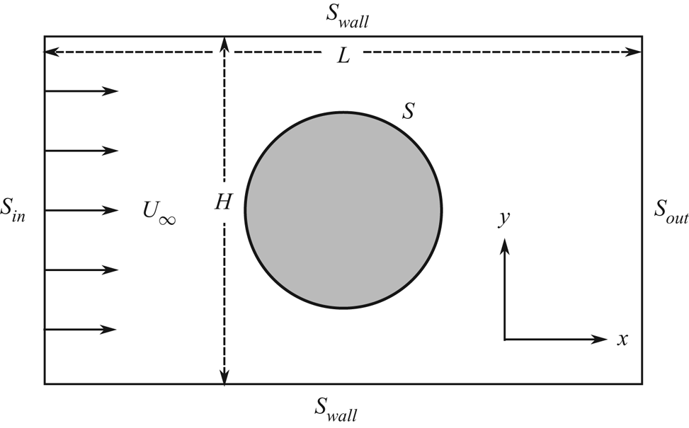
Laboratory experiments and numerical simulations (Dutka et al. Reference Dutka, Starchenko, Osselin, Magni, Szymczak and Ladd2020) used a quasi-two-dimensional Hele-Shaw cell, dimensions  $L (38\ \textrm {mm}) \times H (33\ \textrm {mm}) \times d (0.5\ \textrm {mm})$, with a disk of radius
 $R=10\ \textrm {mm}$ blocking the central region of the channel (figure 2). With these proportions, numerical simulations (Dutka et al. Reference Dutka, Starchenko, Osselin, Magni, Szymczak and Ladd2020) show that the dissolution of the disk is essentially two-dimensional, in contrast to taller and thinner cylinders where there is significant variability of shape in the vertical direction (Soulaine et al. Reference Soulaine, Roman, Kovscek and Tchelepi2017; Molins et al. Reference Molins, Trebotich, Arora, Steefel and Deng2019). In the present case diffusion smears out the variation in concentration over the small height of the disk (
 $0.5 \ \textrm {mm}$) and there are negligible differences between the results of two- and three-dimensional simulations. We therefore consider a two-dimensional pore space, sketched in figure 2, bounded by the lines
 $S_{in}$,
 $S_{out}$, and
 $S_{wall}$. A soluble disk, with boundary
 $S$, is located at the centre of the cell (
 $L/2,H/2)$. The fluid velocity along the inlet and outlet lines is constant (
 $U_\infty$), while the upper and lower walls are impermeable, emulating the experimental set-up. By moving the boundaries to distant locations, we can accommodate an isolated disk far from any boundaries.
The flow geometry considered in this paper. The system is two-dimensional with inlet ( $S_{in}$), outlet (
 $S_{out})$ and inert (
 $S_{wall}$) boundaries. The central circle is a thin cylinder of soluble mineral with a dissolving surface (
 $S$).

Fluid flowing under the experimental conditions can be approximated as a lubrication flow, with a vertically averaged velocity  $[u_x,u_y]$ given by
 \begin{equation} \boldsymbol{\nabla} p = \mu \left(\nabla^2{\boldsymbol{u}} - K^{-1}{\boldsymbol{u}} \right), \end{equation}
where  $\mu$ is the viscosity of the fluid and the pressure
 $p$ is determined by the incompressibility condition,
 \begin{equation} \boldsymbol{\nabla} \boldsymbol{\cdot} {\boldsymbol{u}} = 0. \end{equation}
The drag force density from the top and bottom plates,  $\mu K^{-1} {\boldsymbol {u}}$, must be included in the two-dimensional momentum balance; the effective permeability in the experimental cell
 $K = d^2/12 \approx 0.0208 \ \textrm {mm}^2$. The Reynolds number is small (
 $Re = U_\infty d / \nu < 0.01$), so inertial terms can be neglected.
Transport of reactants follows a convection–diffusion equation
 \begin{equation} \boldsymbol{\nabla} \boldsymbol{\cdot} ({\boldsymbol{u}} c) = D \nabla^2c, \end{equation}
where  $c$ is the cup-averaged concentration field (Bird, Stewart & Lightfoot Reference Bird, Stewart and Lightfoot2001) and
 $D$ is the molecular diffusion coefficient. Since dissolution of the solid is extremely slow in comparison with the time scales for reactant transport (Szymczak & Ladd Reference Szymczak and Ladd2012; Starchenko et al. Reference Starchenko, Marra and Ladd2016), the stationary limit of the convection–diffusion equation is sufficient. Dissolution of calcium sulphate is well described by a linear rate law in the undersaturation (Colombani Reference Colombani2008)
 \begin{equation} {\mathcal{R}}(c_S) = k(c_{sat}-c_S), \end{equation}
where  $c_S$ is the concentration on the mineral surface (
 $S$) and
 $k$ is the surface-reaction-rate constant. The boundary condition on
 $S$ can be found by matching the diffusive and reactive fluxes,
 \begin{equation} {\mathcal{R}}(c_S) = -D ({\boldsymbol{n}} \boldsymbol{\cdot} \boldsymbol{\nabla} c)|_S, \end{equation}
where the normal vector  ${\boldsymbol {n}}$ points into the fluid domain. In the limit of fast surface reactions, the concentration boundary condition reduces to a Dirichlet condition
 \begin{equation} c_S = c_{sat}, \end{equation}
where  $c_{sat} = 15.2 \ \textrm {M} {\ \rm m}^{-3}$ is the saturation concentration of
 $\textrm {CaSO}_4$ (Christoffersen & Christoffersen Reference Christoffersen and Christoffersen1976). Although the dissolution of gypsum is hindered by surface kinetics, in the experimental geometry its effect on the overall dissolution time scale is modest, of the order of 20 % (Dutka et al. Reference Dutka, Starchenko, Osselin, Magni, Szymczak and Ladd2020).
The concentration flux controls the (normal) motion of the surface points,
 \begin{equation} c_{sol}\frac{\mathrm d {\boldsymbol{x}}}{\mathrm d t} = D {\boldsymbol{n}} ({\boldsymbol{n}} \boldsymbol{\cdot} \boldsymbol{\nabla} c)|_S, \end{equation}
where  $c_{sol} = (1-\phi )/v_M$ is the molar concentration of the mineral phase, which had a measured porosity
 $\phi = 0.61$ (Dutka et al. Reference Dutka, Starchenko, Osselin, Magni, Szymczak and Ladd2020), while
 $v_M = 74.4 \times 10^{-6} {\ \rm m}^3 \ \textrm {M}^{-1}$ is the molar volume of the crystalline mineral. The characteristic time scale
 $\tau = R/(U_\infty \gamma )$ is
 $57.3 \ \textrm {h}$; here
 $\gamma = c_{sat}/c_{sol} = 0.0029$ is the ratio of molar concentrations of aqueous and (porous) solid phases. With the experimental flow rate (
 $1\ \textrm {ml}\ \textrm {h}^{-1}$) the Péclet number
 ${Pe = U_\infty R/D = 250}$. The activity-corrected diffusion coefficient,
 $D = 6.75 \times 10^{-4} \ \textrm {mm}^2 \ \textrm {s}^{-1}$, is used to account for the high ionic strength (
 ${\approx } 40 \ \textrm {mM}$) of the nearly saturated solution near the disk (Dutka et al. Reference Dutka, Starchenko, Osselin, Magni, Szymczak and Ladd2020). We have solved these equations, including the effects of confinement, using a finite-volume method (Starchenko et al. Reference Starchenko, Marra and Ladd2016; Starchenko & Ladd Reference Starchenko and Ladd2018); results of these simulations are shown in figures 5 and 6.
It is useful to make the variables dimensionless with the following scalings:
 \begin{equation} {\boldsymbol{x}} \rightarrow \frac{{\boldsymbol{x}}}{R},\quad {\boldsymbol{u}} \rightarrow \frac{{\boldsymbol{u}}}{U_\infty},\quad t \rightarrow \frac{t}{\tau} = \frac{U_\infty \gamma t}{R},\quad c \rightarrow \frac{c_{sat} - c}{c_{sat}},\quad \phi = - \frac {Kp}{U_\infty \mu R}. \end{equation}
The dimensionless governing equations are then
 \begin{gather} {\boldsymbol{u}} - K \nabla^2 {\boldsymbol{u}} = \boldsymbol{\nabla} \phi,\quad \nabla^2 \phi = 0, \end{gather}
 \begin{gather}Pe\, {\boldsymbol{u}} \boldsymbol{\cdot} \boldsymbol{\nabla} c = \nabla^2 c,\quad Pe\, \frac{\mathrm d {\boldsymbol{x}}}{\mathrm dt} = -{\boldsymbol{n}} ({\boldsymbol{n}}\boldsymbol{\cdot}\boldsymbol{\nabla} c)|_S, \end{gather}
with boundary conditions on the soluble mineral surface,
 \begin{equation} {\boldsymbol{n}} \boldsymbol{\cdot} \boldsymbol{\nabla} p = 0,\quad {\boldsymbol{u}} = 0,\quad ({\boldsymbol{n}}\boldsymbol{\cdot}\boldsymbol{\nabla} c)|_S = Da_\mathrm{II} c_S. \end{equation}
For the parameters of the experiment ( $k = 4.5 \times 10^{-3} \ \textrm {mm}\ \textrm {s}^{-1}$,
 $R = 10\ \textrm {mm}$,
 $D = 6.75 \times 10^{-4} \ \textrm {mm}^2 \ \textrm {s}^{-1}$), the second Damköhler number
 $Da_\mathrm {II} = kR/D = 67$. A uniform flow along the
 $x$ direction is set up across the inlet (
 $S_{in}$) and outlet (
 $S_{out}$) boundaries, with
 $c=1$ at the inlet and
 ${\boldsymbol {n}}\boldsymbol {\cdot }\boldsymbol {\nabla } c=0$ at the outlet (figure 2). The remaining boundaries (
 $S_{wall}$) are no slip, with
 ${\boldsymbol {n}}\boldsymbol {\cdot }\boldsymbol {\nabla } c=0$. Further details of the numerical and experimental methods can be found in Dutka et al. (Reference Dutka, Starchenko, Osselin, Magni, Szymczak and Ladd2020).
3. Time dependence of the conformal map
In order to apply conformal-mapping techniques, fluid motion must be reduced to a potential flow. Fortunately, the dimensionless permeability ( $K = d^2/12R^2 \approx 2 \times 10^{-4}$) is small in the experimental geometry, and the shear stress is therefore negligible outside a thin boundary layer around the disk. The Laplacian term in the momentum equation (2.9a,b) will be neglected, in order to maintain a potential flow within the entire fluid domain. Furthermore, we will assume that the chemical reactions on the mineral surface are rapid in comparison with ion diffusion, so that the boundary condition for the concentration (2.11a–c) can be replaced by
 $c_S=0$. The errors introduced by the assumptions of potential flow and fast reactions will be considered in § 4.2.
The dimensionless equations and boundary conditions (2.9a,b)–(2.11a–c), with  $K=0$ and
 $c_S=0$, can be written in complex notation
 \begin{gather} \bar {{\nabla}}_z {{\nabla}}_z \phi = 0, \end{gather}
 \begin{gather}\textrm{Re}\left[Pe\,(\bar {{\nabla}}_z \phi) ({{\nabla}}_z c)\right] = \bar {{\nabla}}_z {{\nabla}}_z c, \end{gather}
 \begin{gather}Pe \frac{\textrm{d} z_b}{\textrm{d} t} = -n_z \textrm{Re}\left[\bar n_z {{\nabla}}_z c\right]|_{z=z_b}; \end{gather}
 \begin{gather}\textrm{Re}\left[\bar n_z {{\nabla}}_z \phi\right] = 0,\quad c = 0,\quad z \in z_b, \end{gather}
 \begin{gather}\phi \rightarrow \textrm{Re}\left[z\right],\quad c \rightarrow 1,\quad z \rightarrow \infty. \end{gather}
The variable  $z = x + \textrm {i}y$ identifies locations in the physical domain and
 $z_b$ marks spatial positions along the mineral–fluid boundary (
 $S$); the subscript
 $z$ indicates gradients and normals in the physical (
 $z$) domain. Although the concentration field is not a harmonic function, the advection–diffusion equation (3.2) is nevertheless conformally invariant (Bazant Reference Bazant2004), and takes the same form in any domain that can be related to the physical one by a conformal mapping. The conformal invariance of (3.1), (3.2), (3.4a–c) and (3.5a–c) allows for a solution of the transport problem in a domain of our choosing, with the mapping function only entering into the evolution of the boundary (3.3).
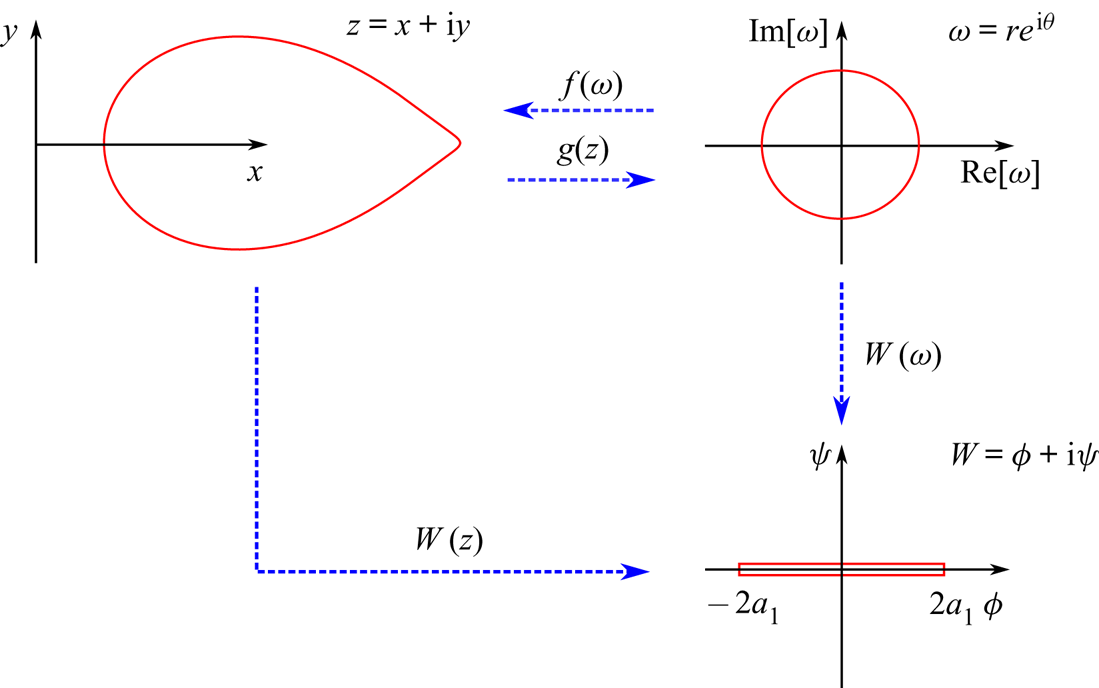
An analytic function  $f(\omega )$ maps the exterior of the unit circle
 $\omega = r\,\textrm {e}^{\textrm {i}\theta }$ to the physical domain,
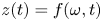 $z(t) = f(\omega , t)$, with a boundary
 $z_b(t) = f(\omega _b, t)$; the inverse mapping is defined by
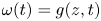 $\omega (t) = g(z, t)$. In § 5 we introduce an auxiliary domain
 $W = \phi + \textrm {i}\psi$, which is the exterior of a finite length slit;
 $\phi$ and
 $\psi$ are the velocity potential and stream function respectively. The connections between the physical domain (
 $z$) and the two mathematical domains (
 $\omega$ and
 $W$) are shown in figure 3. Derivatives of the mapping functions
 $g^\prime (z) = 1/f^\prime (g(z))$ can be used to relate gradients in the physical and mathematical domains,
 ${ {\nabla }}_z = \overline {g^\prime } {{\nabla }}_w$ (Needham Reference Needham2000). We will frequently suppress the time dependence of the mapping function, because it does not enter into the calculation of the flux but only into the evolution of the mapping function itself.
Illustration of the conformal mappings; the boundary of the object in the different domains is indicated by the red lines. The flow creates an asymmetry in the disk, but at high Péclet numbers the solution can be simplified by a conformal mapping from the physical domain  $z$ to the exterior of the unit circle
 $\omega = g(z)$. The function
 $f(\omega )$ maps back from the unit circle to the physical domain. In § 5 we exploit a general solution for advection–diffusion around an absorbing slit (length
 $4a_1$), which can be mapped from the physical domain using the complex potential
 $W = \phi + \textrm {i} \psi$; this domain can also be reached from the unit circle with the mapping
 $W(\omega ) = a_1(\omega + \omega ^{-1})$. The coefficient
 $a_1$ is the conformal radius (3.11); it reflects the size of the solid object in the physical domain.

The velocity potential around a unit disk takes the simple form (Bazant Reference Bazant2004),
 \begin{equation} \phi = \textrm{Re}\left[\omega + \omega^{-1}\right], \end{equation}
which on the surface of the disk is just  $\phi (\omega _b) = 2 \cos \theta$. The flux of aqueous ions leaving the mineral surface can be calculated in the mathematical domain using the relation
 $n_\omega = n_z g^\prime /|g^\prime |$,
 \begin{equation} \textrm{Re}\left[\bar n_z {{\nabla}}_z c\right]|_{z=z_b} = |g^\prime(z)| \textrm{Re}\left[\bar n_\omega {{\nabla}}_\omega c\right]_{|\omega|=1} = \frac{\sigma(\omega_b)}{|\,f^\prime(\omega_b)|}, \end{equation}
where the factor  $|g^\prime | = |\,f^\prime |^{-1}$ compensates for the change in metric under the conformal mapping. The flux around the unit circle can be obtained from the radial derivative of the concentration,
 \begin{equation} \sigma(\omega_b) = (\partial_r c)_{r=1}, \end{equation}
and the velocity of the boundary points from (3.3) is
 \begin{equation} \dot z_b = - \frac{\omega_b \sigma(\omega_b)}{Pe\, \overline{f^\prime(\omega_b)}}. \end{equation}
A marker point on the boundary moves simultaneously in both the physical and mathematical domains; for an individual Lagrangian point both  $z_b$ and
 $\omega _b$ are time dependent (Bensimon et al. Reference Bensimon, Kadanoff, Liang, Shraiman and Tang1986; Feigenbaum, Procaccia & Davidovich Reference Feigenbaum, Procaccia and Davidovich2001). Expressing
 $\dot z_b$ in (3.9) through the mapping function,
 $z_b(t) = f(\omega _b(t), t)$, leads to a generalized Polubarinova–Galin (PG) equation for the evolution of
 $f$ (Goldstein & Reid Reference Goldstein and Reid1978; Bazant et al. Reference Bazant, Choi and Davidovitch2003):
 \begin{equation} \textrm{Re}\left[\overline{\omega_b\,f^\prime(\omega_b, t)} \dot z_b\right] = \textrm{Re}\left[\overline{\omega_b\,f^\prime(\omega_b, t)} \partial_t\,f(\omega_b, t)\right] = -\frac {\sigma(\omega_b)}{Pe}. \end{equation}
The multiplication by  $\bar \omega _b$ eliminates the term proportional to
 $\dot \omega _b$, since
 $|\omega _b|^2 = 1$. The sign is the opposite from Bazant et al. (Reference Bazant, Choi and Davidovitch2003) because it is dissolution rather than precipitation.
3.1. The Laurent hierarchy
The mapping function can be expanded in a Laurent series (Galin Reference Galin1945; Polubarinova-Kochina Reference Polubarinova-Kochina1945; Howison Reference Howison1992; Bazant et al. Reference Bazant, Choi and Davidovitch2003; Rycroft & Bazant Reference Rycroft and Bazant2016)
 \begin{equation} f(\omega, t) = a_1(t) \omega + a_0(t) + a_{-1}(t) \omega^{-1} + \cdots. \end{equation}
In addition to providing a relatively simple solution strategy for the PG equation (3.10), the coefficients  $a_m$ offer physical insight into the size and shape of the evolving solid body. Reflection symmetry about the real (
 $x$) axis implies that the mapping function from the unit circle must also be symmetric,
 $\textrm {Im} [\,f(\bar \omega )]=-\textrm {Im} [\,f(\omega )]$, which requires that the Laurent coefficients
 $a_m$ are all real. The coefficient
 $a_1$ relates the overall size of the solid domain to the radius of the unit circle, and is usually referred to as the conformal radius. The conformal centre
 $a_0$ approximates the shift in the centre of mass when mapping to the real domain. Points within the solid are bounded by the condition
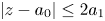 $|z-a_0| \le 2a_1$ (Pommerenke Reference Pommerenke1975), while far from the solid object (
 $|\omega | \rightarrow \infty$)
 $z \sim a_1 \omega$. The flux from (3.7) corresponds to a renormalized flow field in the physical domain, with a far field velocity
 $a_1 U_\infty$. In the mathematical domain the Péclet number must therefore be replaced by the rescaled value
 $Pe\, a_1$, reflecting the decreasing size of the dissolving cylinder; the flux is therefore explicitly time dependent (Bazant et al. Reference Bazant, Choi and Davidovitch2003).
Substituting the Laurent expansion for  $f(\omega )$ (3.11), the evolution of the boundary can be found from (3.10):
 \begin{equation} \textrm{Re} \left[Pe \sum_{m^\prime=-\infty}^1 \sum_{m^{\prime\prime}=-\infty}^1 {m^{\prime} a_{m^\prime} \dot a_{m^{\prime\prime}} \,\textrm{e}^{-\textrm{i}({m^{\prime}}-{m^{\prime\prime}})\theta}} \right] = -\sigma(\theta, t). \end{equation}
The mapping function can be approximated by a finite number of terms, with coefficients found by taking moments 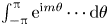 $\int _{-{\rm \pi} }^{{\rm \pi} } \textrm {e}^{\textrm {i}m\theta } \cdots \textrm {d}\theta$ of the evolution equation. For a Laurent series including terms up to
 $\omega ^{-M}$, there are
 $M+2$ unknowns, matched by
 $M+2$ cosine moments
 \begin{equation} \sum_{m^\prime=-M}^1 \sum_{m^{\prime\prime}=-M}^1\,m^{\prime} a_{m^\prime} \dot a_{m^{\prime\prime}} \left[\delta(m-m^\prime+m^{\prime\prime}) + \delta(m+m^\prime-m^{\prime\prime}) \right] = - \frac{\sigma_m(t)}{{\rm \pi} Pe}, \end{equation}
where  $\sigma _m$ are moments of the flux
 \begin{equation} \sigma_m(t) = \int_{-{\rm \pi}}^{\rm \pi} \cos(m\theta) \sigma(\theta, t)\,\textrm{d}\theta. \end{equation}
The coefficients satisfy the differential equations
 \begin{equation} \sum_{m^{\prime}=-M}^{1-m} m^{\prime}a_{m^\prime} {\dot a}_{m^\prime+m} + (m^{\prime}+m)a_{m^\prime+m} {\dot a}_{m^\prime} = s_m, \end{equation}
with  $s_m(t) = -\sigma _m(t)/({\rm \pi} Pe)$ and
 $0 \le m \le (M+1)$. Similar equations have been derived in the low Péclet limit (Rycroft & Bazant Reference Rycroft and Bazant2016), but without assuming a reflection symmetry. However, for symmetric objects we recover the same differential equations as Rycroft & Bazant (Reference Rycroft and Bazant2016), but with right-hand sides that are valid at any Péclet number, not just the asymptotic limits. In this work we examine high Péclet (§ 4) and low Péclet (§ 5.2) asymptotics as well as the general case (§ 5). For small Péclet numbers (
 $Pe \ll 1$) the Laurent series (3.11) can be truncated after the first two terms (§ 5.2) and closed form solutions obtained (Rycroft & Bazant Reference Rycroft and Bazant2016). At
 $Pe=0$, (3.15) reduces to the hierarchy describing Laplacian growth (
 $s_m=\delta _{1,m}$), analysed (for example) by Gustafsson & Vasil'ev (Reference Gustafsson and Vasil'ev2006).
Given an expression for the flux around the unit circle – (4.2), (5.5) or (5.6) – the evolution of the boundary can be found by solving a system of differential algebraic equations (DAEs) of the form  ${\boldsymbol {F}}({\boldsymbol {y}},\dot {\boldsymbol {y}}) = 0$, with initial conditions
 $a_1=1$,
 $a_{m\ne 1} = 0$. Equation (3.15) was implemented as a residual to the IDA solver (https://computing.llnl.gov/projects/sundials), using Python bindings (https://pypi.org/project/Assimulo/) provided by the Assimulo suite (Andersson, Führer & Åkesson Reference Andersson, Führer and Åkesson2015). The IDA implements backwards differencing of variable orders and variable step sizes to maintain the solution within a specified tolerance (
 $10^{-8}$ in this work). Consistent initial conditions, meaning that
 ${\boldsymbol {y}}(0)$ and
 $\dot {\boldsymbol {y}}(0)$ satisfy the DAEs, were implemented by noting that at
 $t=0$ all the coefficients except
 $a_1$ are zero, corresponding to a circular shape. The initial derivatives of the Laurent coefficients are then
 \begin{equation} \dot a_{1-m}(0) = \frac{s_m}{1+\delta_{m,0}}. \end{equation}
Event handling in Assimulo was used to terminate the simulation once the conformal radius was less than twice the specified tolerance.
The area and centre-of-mass position of the dissolving solid can be related to the Laurent coefficients by applying Green's theorem to the complex function  $F(z)$ (Rycroft & Bazant Reference Rycroft and Bazant2016)
 \begin{equation} \iint_A F'(z)\,\textrm{d} x\,\textrm{d} y = -\frac{1}{2\textrm{i}}\oint_C F(z_b)\,\textrm{d}\bar z_b, \end{equation}
where  $A$ is the (two-dimensional) domain bounded by the closed curve
 $C$ and the contour is taken in the counter-clockwise direction. Mapping to the unit circle
 $\omega _b = \textrm {e}^{\textrm {i}\theta }$, the contour integral can be converted to a definite integral,
 \begin{equation} \iint_A F^\prime(z)\,\textrm{d} x \,\textrm{d} y = \tfrac{1}{2}\int_{-{\rm \pi}}^{\rm \pi} F(\,f(\omega_b)) \overline{\omega_b f^\prime(\omega_b)}\,\textrm{d}\theta. \end{equation}
We can use this result to calculate the undissolved area  $A(t)$ (with
 $F(z) = z$), and the location of the centre of mass
 ${\rm \Delta} x(t)$ (with
 $F(z) = z^2/2$), using the Laurent expansion for
 $f(\omega )$ (3.11)
 \begin{gather} A(t) = {\rm \pi}\sum_{{m}=-M}^1\,m a_{m}^2(t), \end{gather}
 \begin{gather}{\rm \Delta} x(t) = \frac{\rm \pi}{2A(t)} \sum_{{m^\prime}=-M}^1 \sum_{{m^{\prime\prime}}=-M}^1 (m^\prime+m^{\prime\prime}) a_{m^\prime+m^{\prime\prime}}(t)a_{m^\prime}(t)a_{m^{\prime\prime}}(t). \end{gather}
4. High  $Pe$ asymptote

In the high Péclet limit ( $Pe \gg 1$), there is an explicit solution for the concentration field outside the unit circle (Bazant Reference Bazant2004).
 \begin{equation} c(r, \theta) = \text{erf} \left( \sqrt{Pe}(r^{1/2}-r^{-1/2})\sin(|\theta|/2) \right). \end{equation}
The polar angle is bounded by  $-{\rm \pi} \le \theta \le {\rm \pi}$, with the downstream stagnation point at
 $\theta =0$ (trailing edge) and the upstream stagnation point at
 $\theta = {\rm \pi}$ (leading edge). Equation (4.1) can be obtained by mapping the solution in the upper half-plane
 $c = \text{erf} (\sqrt {Pe}\ \textrm {Im}[\xi ])$ to the exterior of the unit circle, with the mapping function
 $\omega = \xi ^{1/2}+\xi ^{-1/2}$ (Bazant Reference Bazant2004). The asymptotic character of the solution follows from the mapping function, which imposes a spurious
 $c=0$ condition along the
 $\theta =0$ line behind the disk. At large
 $Pe$ the field values downstream of a given location have a negligible effect on the upstream values; hence the asymptotic character of the solution.
The flux around the unit circle (3.8) can be obtained from the radial derivative of the concentration (4.1),
 \begin{equation} \sigma(\theta,t) = (\partial_r c)_{r=1} = 2\sqrt{\frac{Pe\,a_1(t)}{\rm \pi}} \sin (|\theta|/2), \end{equation}
with moments
 \begin{equation} \sigma_m(t) = \frac{8}{1-4m^2} \sqrt{\frac{Pe\,a_1(t)}{\rm \pi}}. \end{equation}
As discussed in § 3.1, the Péclet number has been replaced by the rescaled value  $Pe\, a_1$, and the flux is therefore explicitly time dependent. Integrating the hierarchy (3.15) with the asymptotic flux moments (4.3) requires 128 Laurent coefficients to obtain the collapse time with six-digit precision. The computations take of the order of 3 minutes.
4.1. Comparison with experiment
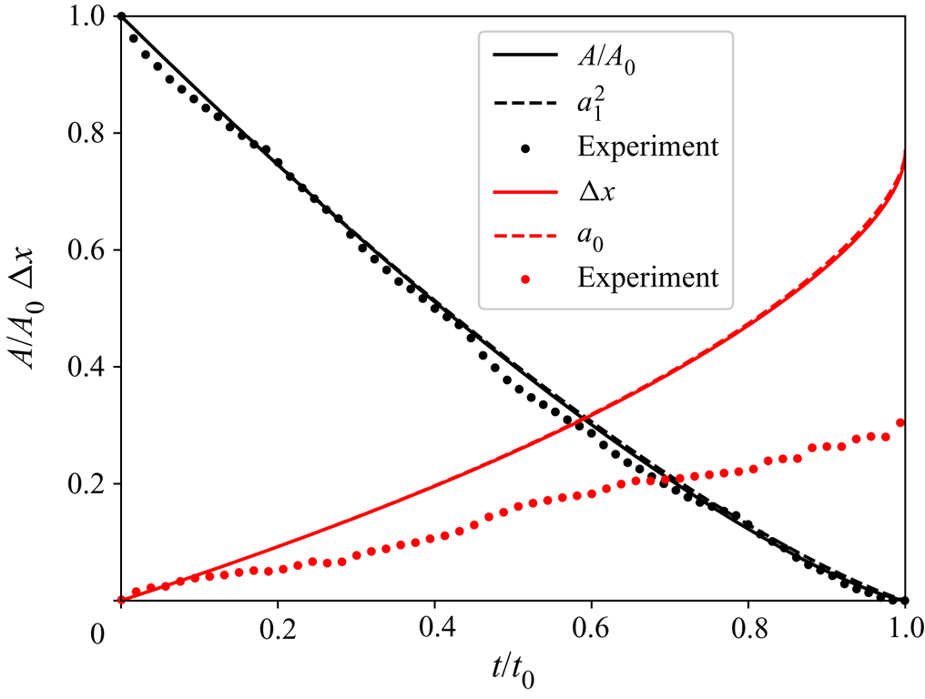
Numerical solutions of the hierarchy (3.15), with the high Péclet flux moments (4.2), lead to a surprisingly close match with experimentally observed shapes (figure 1), despite the differences in fluid flow (viscous versus potential) and boundary conditions. However, solutions from the PG equation were matched to experimental images with the same undissolved area, rather than the same time. Figure 4 includes a comparison of the area of the undissolved solid (3.19) with experimental measurements from Dutka et al. (Reference Dutka, Starchenko, Osselin, Magni, Szymczak and Ladd2020). The time axis is scaled by the collapse time  $t_0$, which is the time taken for complete dissolution of the sample. In the scaled time the areas match to within the uncertainties of the experimental measurements, so that the different underlying physics is reflected only in a change of time scale. The experimental conditions result in a time scale
 $\tau = 57.3 \ \textrm {h}$ (§ 2), while the sample took
 $1000 \ \textrm {h}$ to dissolve completely. The dimensionless collapse time from experiment is therefore
 $t_0 = 17.5$, whereas the collapse time from the PG equation is
 $t_0 = 14.5$. The size and shape of the undissolved solid can therefore be mapped to the experimental observations by a change in time scale of less than 20 %.
The area and shift in centre of mass of a dissolving disk as a function of time. The solid lines are a fully convergent solution ( $M=128$) of the PG equation (3.15), while experimental measurements (Dutka et al. Reference Dutka, Starchenko, Osselin, Magni, Szymczak and Ladd2020) are shown as solid circles. The dashed lines are single moment approximations to (3.19) and (3.20),
 $A/A_0 \approxeq a_1^2$ and
 ${\rm \Delta} x \approxeq a_0$ (§ 4.3). The time scale
 $t_0$ is the collapse time of the disk, when the dissolving solid vanishes entirely:
 $t_0 = 14.5$ from the PG equation versus
 $17.5$ from experiment.

The centre of mass of the disk shifts downstream as it dissolves, but the theoretical prediction is approximately twice as large as the experimentally observed shift (figure 4). Discrepancies in dissolution time scale and drift of the centre of mass have been investigated by numerical simulations and will be discussed in § 4.2. The assumption of potential flow and transport-limited kinetics leads to faster dissolution at the leading edge of the disk than in the experiment, but nevertheless the shapes at matching areas (figure 1) are very similar. We discuss the independence of shape and shift in terms of the Laurent coefficients in §§ 4.3 and 5.3.
We note that the experiment used for figure 4 is not the same as the one shown in figure 1. For figure 1 we selected the experiment with the most regular shapes, but halfway through that experiment the flow rate was quadrupled, changing the time scale. We therefore used another experiment, with a constant flow rate but slightly less regular shapes, for figure 4. A complete description of the experimental results can be found in Dutka et al. (Reference Dutka, Starchenko, Osselin, Magni, Szymczak and Ladd2020); it includes videos of all the experiments, and examples of the images utilized for figures 1 and 4 (figures 11 and 10 respectively from that work).
4.2. Limitations of potential flow and transport-limited kinetics
We have shown in § 4.1 that the differences between the theoretical model described by (3.1)–(3.5a–c) and microfluidic experiments can largely be accounted for by a change in time scale and a shift in the position of the centre of mass; the solid shapes are remarkably similar and the outlines of the boundary overlap almost exactly. Finite-volume simulations of equations enable us to track the effects of the different physics that separates the solutions of (3.1)–(3.5a–c) from the laboratory experiments: Stokes versus potential flow, finite versus infinite Damköhler number and confined versus unbounded systems. The finite-volume simulations are second-order approximations to (2.9a,b)–(2.11a–c), laid out in § 2; the methods have been described in detail elsewhere (Starchenko et al. Reference Starchenko, Marra and Ladd2016; Starchenko & Ladd Reference Starchenko and Ladd2018; Dutka et al. Reference Dutka, Starchenko, Osselin, Magni, Szymczak and Ladd2020).
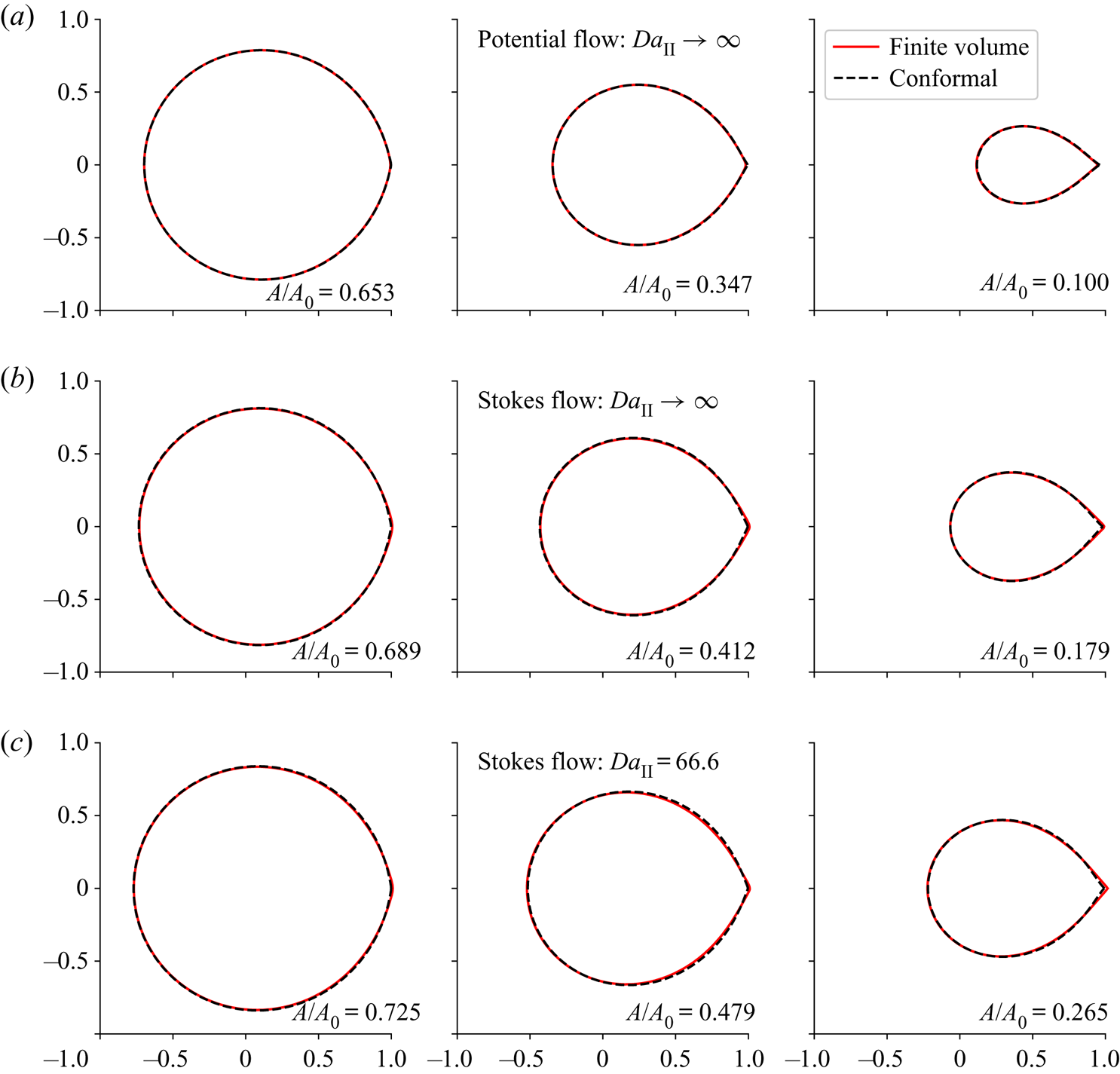
Figure 5 shows the shape of a dissolving disk from finite-volume simulations (red lines) at different dimensionless times ( $t=4, 8, 12$). Images in each row correspond to a particular physical model indicated by the title – potential flow versus Stokes flow and transport-limited dissolution versus a finite reaction rate; the dimensionless time in each column is the same. The black dashed lines are from a conformal mapping of potential flow and transport-limited kinetics in an infinite domain, at times chosen so that the area of the undissolved solid matches that in the finite-volume simulation; those areas are indicated in each panel.
Finite-volume simulations (red lines) of a dissolving disk (Dutka et al. Reference Dutka, Starchenko, Osselin, Magni, Szymczak and Ladd2020) at  $Pe=250$; the simulations are matched with solutions of the Polubarinova–Galin equation (3.15) at the same area. Dimensionless times for the three columns are
 $t=4$,
 $t=8$, and
 $t=12$ respectively, with the time scale from (2.8c). (a) Finite-volume simulations with potential flow and transport-limited kinetics, as used in conformal mapping. A finite-volume simulation with Stokes flow instead of potential flow is shown in (b). (c) Results with the reaction rate characterizing the experiments (
 $k=4.5 \times 10^{-3} \ \textrm {mm} \ \textrm {s}^{-1}$); the Damköhler number
 $Da_\mathrm {II} = k/U_\infty = 66.7$. Solutions of the PG equation (black dashed lines) have been scaled in time and shifted to coincide with the finite-volume simulations. The time scales and shifts are shown in figure 6.

Results from a potential flow simulation, with a slip boundary condition on the surface of the dissolving disk, are shown in figure 5(a). Transport-limited kinetics,  $c({\boldsymbol {r}} \in S)=0$, were used to match the solution from the PG equation. In this case solutions of the PG equation (3.15) need no rescaling of the time or shift in centre of mass to map onto the finite-volume results. The time scale (
 $t_C$) and shift (
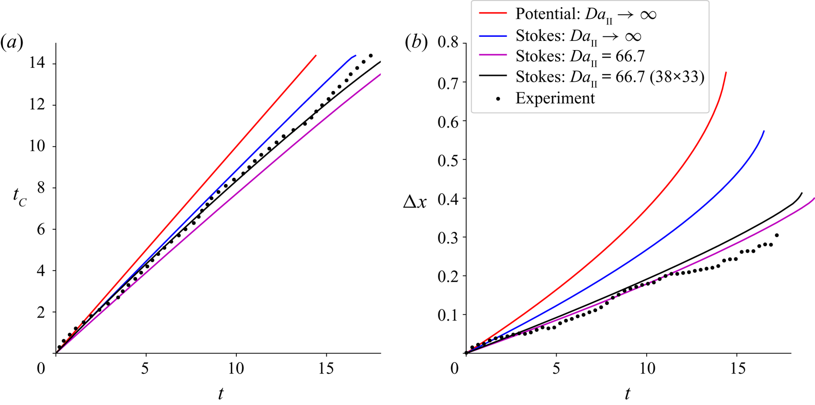
 ${\rm \Delta} x$) exactly match the finite-volume simulation, as indicated by the red line (with a slope of 1) in figure 6(a) and the red line in figure 6(b).
Time scale and centre of mass for different flow and transport equations. (a) The rescaled time ( $t_C$) of the conformal mapping (potential flow,
 $Da_\mathrm {II} \rightarrow \infty$, infinite domain) is compared with the dissolution time scale for different physical models (
 $t$): potential flow,
 $Da_\mathrm {II} \rightarrow \infty$, unbounded domain (red); Stokes flow,
 $Da_\mathrm {II} \rightarrow \infty$, unbounded domain (blue); Stokes flow,
 $Da_\mathrm {II} = 66.7$, unbounded domain (magenta); Stokes flow,
 $Da_\mathrm {II} = 66.7$, finite domain (black). For potential flow (with
 $Da_\mathrm {II} = \infty$ and an unbounded domain) the time scales
 $t_C$ and
 $t$ are the same, so the slope is unity. The decreased slopes for Stokes-flow simulations reflect the slower dissolution in these cases. (b) The shift in centre of mass for different physical models. The black circles are the experimental results; the corresponding simulations are shown by the black lines.

In Stokes flow the fluid velocity on the disk vanishes, which sets up a viscous boundary layer around the disk with a thickness of order  $d$, the gap between the plates of the Hele-Shaw cell. The disk dissolves more slowly than in the potential flow case, as indicated in figure 6(a). In order to match shapes, rescaled times
 $t_C$ were determined by matching areas between solutions of the PG equation and finite-volume simulations
 \begin{equation} A(t_C) = A_{sim}(t). \end{equation}
The linear dependence of  $t_C$ on
 $t$ (figure 6a) shows that there is a single rescaling of the time that enables the shapes from conformal mapping to match those from Stokes-flow simulations. The shift in centre of mass is reduced by switching from potential to Stokes flow (figure 6b) and is more in line with the experimental observations, although the shift (blue line) is still too large.
A closer match with the experimental time scale can be achieved by including a finite surface dissolution rate, which in dimensionless form is given by (2.11a–c). Now the shift in centre of mass closely aligns with the experimental measurements shown in figure 4, although the dissolution is slightly slower (magenta line in figure 6a). The remaining discrepancy can be resolved by using a similar sized Hele-Shaw cell, with dimensions  $3.8 R \times 3.3 R$ as opposed to an unbounded system. This produces a small change in the centre of mass position (black line in figure 6b) but reduces the time for complete dissolution to
 $t_0 = 17.5$ (figure 6a) or
 $1000 \ \textrm {h}$, which precisely matches the experiment.
4.3. Analytic solutions for the low-order Laurent coefficients
Analytical approximations to the Laurent coefficients can be obtained by first truncating the expansion of the mapping function (3.11), beyond the third term. The truncated moment hierarchy from (3.15) becomes
 \begin{gather} -2a_{-1}^0 \dot a_{-1}^0 + 2a_1^0 \dot a_1^0 = -\frac{8}{\sqrt{{\rm \pi}^3 Pe}}\sqrt{a_1^0}, \end{gather}
 \begin{gather}-a_{-1}^0 \dot a_0^0 + a_1^0 \dot a_0^0 = \frac{8}{3\sqrt{{\rm \pi}^3 Pe}}\sqrt{a_1^0}, \end{gather}
 \begin{gather}-a_{-1}^0 \dot a_1^0 + a_1^0 \dot a_{-1}^0 = \frac{8}{15\sqrt{{\rm \pi}^3 Pe}}\sqrt{a_1^0} . \end{gather}
The zero superscript denotes approximate solutions for  $a_m$ from the three-term expansion of
 $f$. Noticing that
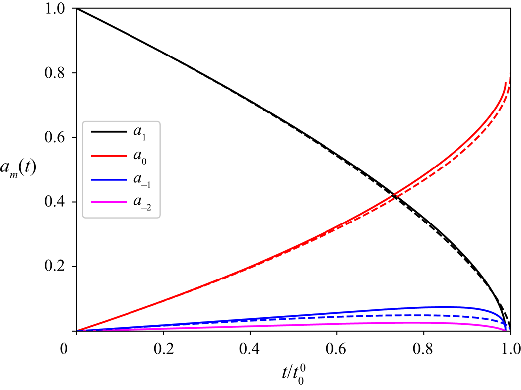
 $a_1$ (solid black line in figure 7) is significantly larger that
 $a_{-1}$ (solid blue line in figure 7), we can solve for
 $a_1^0$ by neglecting the small term
 $2a_{-1}^0\dot a_{-1}^0$ in (4.5),
 \begin{equation} a_1^0(t) = \left(1 - \frac{t}{t_0^0}\right)^{2/3}. \end{equation}
The collapse time, when  $a_1^0$ vanishes,
 \begin{equation} t_0^0 = \frac{\sqrt{{\rm \pi}^3 Pe}}{6} = 14.674 \end{equation}
is within  $1\,\%$ the exact (
 $M = 128$) value,
 $t_0 = 14.506$. There are only small differences between the exact numerical solution for
 $a_1$ (solid black line) and the approximate result
 $a_1^0$ (dashed black line), mostly near the collapse point; the exact coefficient
 $a_1$ vanishes at
 $t_0$, while the analytical approximation
 $a_1^0$ vanishes at
 $t_0^0$, which is approximately 1 % larger.
Time-dependent Laurent coefficients at  $Pe=250$. The solid lines are numerical results with
 $M = 128$. The time has been scaled by the analytical collapse time
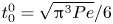 $t_0^0 = \sqrt {{\rm \pi} ^3 Pe}/6$; the numerical collapse time
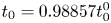 $t_0 = 0.98857t_0^0$. The dashed lines are the analytical approximations from (4.8) and (4.12a,b).

The remaining coefficients can be found by replacing the time variable in (4.6) and (4.7) by  $a_1^0$, noting that
 $\dot a_1^0 = -2/(3t_0^0 \sqrt {a_1^0})$
 \begin{gather} \left(-a_{-1}^0+a_1^0\right) \frac{\textrm{d} a_0^0}{\textrm{d} a_1^0} = -\frac{2}{3}a_1^0, \end{gather}
 \begin{gather}-a_{-1}^0+a_1^0 \frac{\textrm{d} a_{-1}^0}{\textrm{d} a_1^0} = -\frac{2}{15}a_1^0. \end{gather}
Solving first for  $a_{-1}^0$ and then for
 $a_0^0$, the solutions in terms of
 $a_1^0$ are
 \begin{equation} a_0^0 = 5 \exp(-15/2)\left[\text{Ei}(15/2)-\text{Ei}(15/2+\ln a_1^0) \right],\quad a_{-1}^0 = -\tfrac{2}{15}a_1^0 \ln a_1^0, \end{equation}
where  ${\text{Ei}(x)} = -\int _{-x}^{\infty } t^{-1}\,\textrm {e}^{-t}\,\textrm {d} t$ is the exponential integral function. The analytical solutions from (4.12a,b) are compared with numerical results (
 $M = 128$) in figure 7. There are only small differences in centre of mass (red lines) between the numerical (solid) and analytical (dashed) results. At the collapse point (
 $t=t_0^0$)
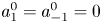 $a_1^0 = a_{-1}^0 = 0$, while the shift in centre of mass reaches a constant value close to the numerical one,
 $a_0^0 = 5 \exp(-15/2)\text{Ei}(15/2) = 0.800$. The discrepancy in
 $a_{-1}^0$ (blue lines) in figure 7 comes from the neglect of higher-order Laurent coefficients (
 $m < -1$), rather than the approximation for
 $a_1^0$.
4.4. Time-dependent area and centre of mass
In § 4.2, we noted that the impact of potential flow and transport-limited kinetics was largely restricted to the time dependence of the area of the solid domain and the shift in its centre of mass (figure 6); the shapes at the same area were similar for the different physical models (figure 5). Here we examine the time dependence of the conformal area ( $a_1$) and centre (
 $a_0$), which are closely connected to the area and centre of mass of the disk. Figure 4 shows that approximations to the area and centre of mass derived from the first two coefficients in the Laurent expansion (dashed lines) are almost indistinguishable from the exact results (solid lines). Taking the terms involving just
 $m = 0$ and
 $m=1$ from (3.19) and (3.20), we have:
 \begin{equation} \frac{A}{A_0} \approxeq a_1^2,\quad {\rm \Delta} x \approxeq a_0. \end{equation}
The area corresponds approximately to the square of the conformal radius, whereas the centre-of-mass position corresponds to the conformal centre.
Equations (4.13a,b) and (4.8) imply that the area of the object will decrease as  $(1-t/t_0^0)^{4/3}$. The scaling is not exact, but a comparison of the solid and dashed black lines in figures 4 and 7 shows that it is very close. Interestingly a similar scaling is predicted for mechanical erosion at large Reynolds numbers (Moore et al. Reference Moore, Ristroph, Childress, Zhang and Shelley2013), despite the different mechanisms for material removal. Erosion of friable materials such as clay (Ristroph et al. Reference Ristroph, Moore, Childress, Shelley and Zhang2012) is due to the large shear stresses on the solid surface caused by the flowing fluid. On the other hand, dissolution is a result chemical reactions at the solid surface. However, the interplay of convection and diffusion, momentum in one case (erosion) and mass in the other (dissolution), may offer an explanation for the similarity in the scaling of the area.
In contrast to the shapes in figure 1, with the cusp pointing downstream, erosion produces objects with the cusp pointing upstream (Ristroph et al. Reference Ristroph, Moore, Childress, Shelley and Zhang2012). Nevertheless, in both cases the flux scales as  $\sqrt {U_\infty /a_1}$, which is also the case for dissolution at large
 $Re$ (Huang et al. Reference Huang, Moore and Ristroph2015). This gives a general scaling relation for the evolution of the conformal radius
 $\dot a_1 \sim a_1^{-1/2}$ which leads to (4.8). The area of two-dimensional bodies then scales as
 $(1-t/t_0)^{4/3}$ (Moore et al. Reference Moore, Ristroph, Childress, Zhang and Shelley2013), while the volume of three-dimensional bodies scales as
 $(1-t/t_0)^2$ (Huang et al. Reference Huang, Moore and Ristroph2015). However, at low Péclet numbers the area decays approximately linearly in time (§ 5.2) for both dissolution (Rycroft & Bazant Reference Rycroft and Bazant2016) and erosion (Quaife & Moore Reference Quaife and Moore2018).
4.5. Motion of the leading and trailing edges
The position and curvature of the boundary near the leading ( $\theta = {\rm \pi}$) and trailing (
 $\theta = 0$) edges can be written in terms of cumulants of the Laurent coefficients,
 \begin{equation} S_n^\pm(t) = \sum_{m=-M}^1 (\pm 1)^m m^n a_m(t), \end{equation}
where the minus sign refers to the leading edge, and the plus sign to the trailing edge. The positions and curvatures are given by
 \begin{equation} z_b^\pm = S_0^\pm,\quad C_b^\pm = \frac{\textrm{d}^2x/\textrm{d}\theta^2}{(\textrm{d} y/\textrm{d}\theta)^2} = - \frac{S_2^\pm}{(S_1^\pm)^2}. \end{equation}
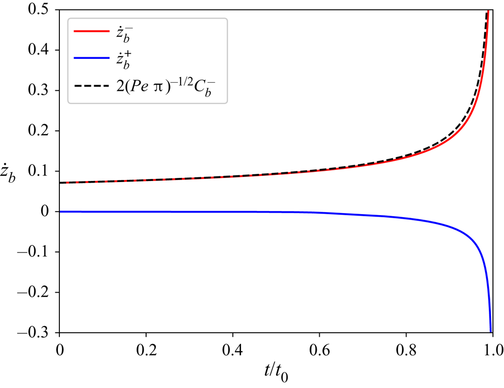
The velocity of the leading edge increases slowly at first and then more rapidly, as shown in figure 8. Similarly to a parabolic tip (Cummings et al. Reference Cummings, Hohlov, Howison and Kornev1999), the velocity of the leading edge is proportional to the square-root of the curvature. The multiplicative factor,  ${2/\sqrt {Pe\,{\rm \pi} }}$, can be found by summing the time derivatives of the coefficients
 \begin{equation} \dot {S}_0^-(0) = \sum_{m=-M}^1 (-1)^m \dot{a}_m(0) = \frac{4}{3 t_0^0}\left(\tfrac{1}{2}+\sum_{m=1}^\infty (-1)^{m-1}\frac{1}{4m^2-1}\right) =\frac{2}{\sqrt{Pe\,{\rm \pi}}}, \end{equation}
where  $\dot {a}_m(0)$ given by (3.16). It is larger than the velocity of a parabolic tip (Cummings et al. Reference Cummings, Hohlov, Howison and Kornev1999) by a factor of
 $\sqrt {2}$, but consistent with the flux at the leading edge of the circle (4.2). The connection between velocity and curvature is approximately maintained at later times, as shown in figure 8.
Velocity of the leading and trailing edges,  $\dot {z}_b^\pm$, at
 $Pe=250$ (
 $M = 128$); the plus sign refers to the trailing edge and the minus sign to the leading edge. The curvature of the leading edge (4.15b) is shown as the dashed black line.

By contrast, the trailing edge is essentially stationary ( $\dot {S}_0^+(0)=0$) until late in the dissolution, when the effective Péclet number,
 $a_1(t) Pe$, is small. In reality the trailing edge has a small velocity even at
 $t=0$ (§ 5); however, a limitation of the asymptotic approximation is that the flux at the trailing edge is predicted to vanish (4.1), whereas in fact it takes a constant value of
 $1/{\rm \pi}$ (Choi et al. Reference Choi, Margetis, Squires and Bazant2005). However, these differences are not significant when making comparisons with the experiment, given the uncertainties in the data.
5. Solutions for arbitrary Péclet number
The high Péclet asymptotic approximation (§ 4), is valid in the region  $\theta \gg Pe^{-1/2}$ (Choi et al. Reference Choi, Margetis, Squires and Bazant2005). Near the trailing tip,
 $\theta \ll Pe^{-1/2}$, the flux takes a different form from (4.2),
 $\sigma \rightarrow 1/{\rm \pi}$. However, an exact conformal mapping can be derived from a Boussinesq transformation, which uses the velocity potential
 $\phi$ and stream function
 $\psi$ as coordinates. The physical domain
 $z \in {\mathcal {R}}^2$ is mapped to the
 $\phi$–
 $\psi$ plane with the complex function
 $W(z) = \phi (z) + \textrm {i} \psi (z)$, as illustrated in figure 3. The stream function
 $\psi$ is constant along the boundary of the disk and can be taken to be zero. The boundary of the dissolving disk then maps to a slit along the real axis (
 $\phi , \psi =0)$, with
 $-2a_1 \le \phi \le 2a_1$. The parameter
 $a_1 < 1$ is time dependent (with
 $a_1(0) = 1$), reflecting the shrinking scale of the object; determining
 $a_1(t)$ is again part of the calculation.
A new function  $C(\phi ,\psi ) = \textrm {e}^{-Pe \phi /2}[1-c(\phi ,\psi )]$ satisfies the Helmholtz equation
 \begin{equation} \partial_\phi^2 C + \partial_\psi^2 C = (Pe/2)^2 C, \end{equation}
with boundary conditions (Goldstein & Reid Reference Goldstein and Reid1978)
 \begin{gather} C = \textrm{e}^{-Pe \phi/2},\quad -2a_1 \le \phi \le 2a_1,\quad \psi = 0, \end{gather}
 \begin{gather}C \rightarrow 0,\quad \phi^2 + \psi^2 \rightarrow \infty. \end{gather}
The solution of (5.1)–(5.3a,b) can be found by solving an integral equation for the flux  $(\partial _\psi c )_{\psi =0}$,
 \begin{equation} {\rm \pi}= \int_{-2a_1}^{2a_1} K\left[\tfrac{1}{2}Pe(\phi-\phi^\prime)\right]\left(\partial_\psi c \right)_{\psi=0}, \textrm{d} \phi^\prime, \end{equation}
where the kernel  $K(x) = \textrm {e}^x K_0(|x|)$ and
 $K_0$ is a modified Bessel function. This approach was first used by Goldstein & Reid (Reference Goldstein and Reid1978), who applied it to the evolution of a frozen domain with a heat sink at the origin. They calculated a series of shapes similar to those shown in figure 5. Subsequently, Kornev & Mukhamadullina (Reference Kornev and Mukhamadullina1994) solved for the steady-state shape of the frozen region directly. These problems involve both a fluid region with convection diffusion (as here), but also a coupled interior region with a Laplacian temperature field. In our case there is only the exterior domain but the same method can be used to calculate the concentration flux on the surface.
The integral equation can be transformed to the unit circle  $\omega _b = \textrm {e}^{\textrm {i} \theta }$ by the mapping function
 $W(\omega _b) = a_1(\omega _b + \omega _b^{-1})$. The (real) mapping function for the boundary is just the velocity potential on a circle of radius
 $a_1$,
 $\phi = 2a_1 \cos \theta$. From the mapping function
 $W(\omega _b)$, we have
 $\textrm {d}\phi + \textrm {i}\textrm {d}\psi = 2a_1 \sin \theta (-r \textrm {d}\theta + \textrm {i} \textrm {d} r)$, and the integral equation can be transformed to the
 $\theta$ coordinate,
 \begin{equation} {\rm \pi}= \int_{0}^{\rm \pi} K\left[\lambda(\cos\theta-\cos\theta^\prime)\right]\sigma(\theta^\prime)\,\textrm{d} \theta^\prime, \end{equation}
where  $\lambda = Pe\, a_1$ and the flux
 $\sigma (\theta ) = \partial _r c(r,\theta )|_{r=a_1}$. The flux in (4.2) is the high Péclet limit of (5.5) (Goldstein & Reid Reference Goldstein and Reid1978).
It is preferable to solve the integral equation on the circle (5.5) rather than the slit (5.4) because the flux is well behaved; for  $\theta \gg Pe^{-1}$,
 $\sigma \sim \sin |\theta |/2$, while for
 $\theta \ll Pe^{-1}$,
 $\sigma \sim {\rm \pi}^{-1}$ (Choi et al. Reference Choi, Margetis, Squires and Bazant2005). On the other hand, the flux in (5.4) is singular at
 $\phi = \pm 1$. Given a numerical representation of the flux (appendix A), we can solve for the evolution of the disk as in § 4; the Laurent coefficients are calculated by numerical integration over the perimeter of the circle. In this case the flux
 $\sigma (\theta , t)$ must be recalculated at every time step, because the Péclet number is no longer just a scaling parameter. Nevertheless, a typical simulation, with
 $M=32$ and 128 quadrature points, takes approximately 10 minutes to integrate to the collapse point; this level of approximation is sufficient to predict the collapse time
 $t_0$ to 5 significant figures. The remaining figures were generated using 34 Laurent coefficients to represent the mapping function (
 $M=32$); the collapse time with
 $M=64$ differs by less than one part in
 $10^5$. The more rounded tip may reduce the dependence of the shape on the number of Laurent coefficients in comparison with calculations using the high
 $Pe$ asymptotic flux.
5.1. Shapes of a dissolving disk at different Péclet numbers
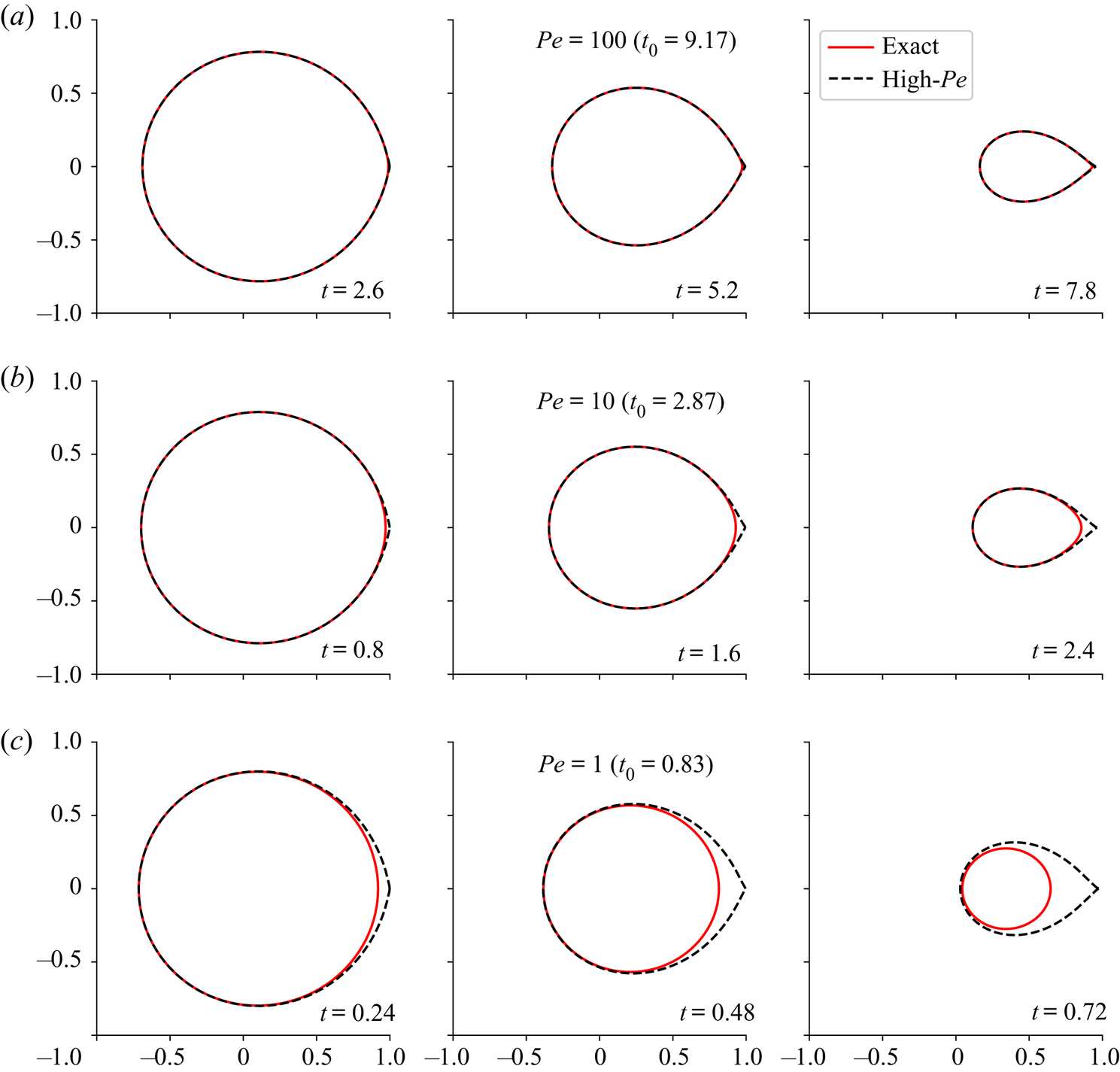
The shapes of a dissolving disk have been calculated for different initial Péclet numbers ( $Pe$); the results are summarized in figure 9. At sufficiently large Péclet numbers (
 $Pe > 100$), the shapes derived from the asymptotic flux (3.8) are almost indistinguishable from the exact shapes from (5.5) (figure 9a). The sequence of shapes is independent of
 $Pe$, with a dimensionless time scale proportional to
 $\sqrt {Pe}$. Since time was made non-dimensional by the fluid velocity (2.8c), the physical time scale is proportional to
 $Pe^{-1/2}$.
Dissolution in potential flow by an exact conformal mapping (red solid lines) and the high Péclet asymptotic approximation (black dashed lines). Results are shown at different dimensionless times and at Péclet numbers:  $Pe = 100$ (a),
 $Pe = 10$ (b) and
 $Pe = 1$ (c). The time for complete dissolution
 $t_0$ derived from the exact conformal mapping is shown in parentheses.

The disk develops a cusp at the trailing edge, which becomes more pronounced as it dissolves. This shape is characteristic of dissolution experiments and simulations at low  $Re$, but high
 $Pe$ (Soulaine et al. Reference Soulaine, Roman, Kovscek and Tchelepi2017; Dutka et al. Reference Dutka, Starchenko, Osselin, Magni, Szymczak and Ladd2020). The fluid near the trailing edge is nearly saturated with mineral ions and the disk dissolves much more slowly here than on the leading edge. The slow dissolution of the trailing edge also accounts for the positive shift in the centre of mass (figure 4). There does not seem to be an asymptotic shape where only the size (
 $a_1$) and centre (
 $a_0$) are time varying. Instead, the tip is constantly evolving in a history dependent manner. Interestingly, high Péclet precipitation does have an invariant shape (Davidovitch et al. Reference Davidovitch, Choi and Bazant2005), although it is not known what initial conditions lead to that shape. We were unable to find a similar factorization for the mapping function of a dissolving object, and numerical results show that an invariant shape does not evolve from an initially circular disk.
By contrast, dissolution at high Reynolds numbers results in a flat trailing edge, due to enhanced mixing in the wake behind the object (Huang et al. Reference Huang, Moore and Ristroph2015). The leading edge of a dissolving cylinder (or sphere) has a finite radius of curvature (Huang et al. Reference Huang, Moore and Ristroph2015), as it does at low  $Re$. On the other hand, erosion at high Reynolds number leads to a triangular-shaped tip with straight edges meeting at approximately
 $90^\circ$ (Ristroph et al. Reference Ristroph, Moore, Childress, Shelley and Zhang2012; Moore et al. Reference Moore, Ristroph, Childress, Zhang and Shelley2013).
At lower  $Pe$, (3.8) incorrectly predicts a cusp at the trailing edge, while the exact solution is more egg shaped (figure 9b). Furthermore, the asymptotic flux does not capture the persistent circular shape when
 $Pe < 1$ (figure 9c). The circular shape at low Péclet (
 ${Pe < 1}$) has been found previously (Rycroft & Bazant Reference Rycroft and Bazant2016), using a low Péclet asymptotic expansion. The numerical approach outlined in this section is uniformly valid over the whole range of Péclet numbers, and smoothly connects the low and high-
 $Pe$ asymptotes. In § 5.2 we improve on the low Péclet expansion in Rycroft & Bazant (Reference Rycroft and Bazant2016) by including logarithmic (in
 $Pe$) contributions to the flux.
5.2. Low Péclet limit
At low Péclet numbers there is an asymptotic expansion of (5.4) for which the leading terms are (Choi et al. Reference Choi, Margetis, Squires and Bazant2005)
 \begin{equation} \sigma(\theta, t) = \frac{1 + (1-C)Pe\, a_1(t)\cos \theta + {\textit{O}}(Pe^2)}{C}; \end{equation}
here,  $C(t) = -\gamma - \ln (Pe\, a_1(t)/4)$ and
 $\gamma$ is Euler's constant.
The flux (5.6) has only two moments up to linear order in  $Pe$: from (3.14)
 \begin{equation} \sigma_0 = 2{\rm \pi} C^{-1},\quad \sigma_1 = {\rm \pi}Pe\, a_1 (C^{-1}-1). \end{equation}
With the low- $Pe$ flux (5.6), (4.5)–(4.7) are
 \begin{gather} -2a_{-1} \dot a_{-1} + 2a_1 \dot a_1 = -\frac{2C^{-1}(t)}{Pe}, \end{gather}
 \begin{gather}-a_{-1} \dot a_0 + a_1 \dot a_0 = -a_1(C^{-1}(t)-1), \end{gather}
 \begin{gather}-a_{-1} \dot a_1 + a_1 \dot a_{-1} = 0 . \end{gather}
If the disk is initially circular,  $a_{-1} = 0$ for all times (since
 $\dot a_{-1} \propto a_{-1}$); in fact, if we ignore contributions to the flux from order
 $Pe^2$ and above, all the Laurent coefficients other than
 $a_0$ and
 $a_1$ are zero. Taking
 $m = -M$ in (3.15), we find from an equation similar to (5.10) that
 $a_{-M} = 0$. Working up through the hierarchy (3.15), with successively decreasing values of
 $m$, it can be seen that all the coefficients up to
 $a_0$ vanish.
In order to analyse the dissolution of complex shapes, Rycroft & Bazant (Reference Rycroft and Bazant2016) argued that the logarithmic term in  $C$ could be assumed constant,
 $C(t) = C_0 = -\gamma - \ln (Pe/4)$. In that case, the area and shift depend linearly on time (Rycroft & Bazant Reference Rycroft and Bazant2016), with a collapse time and final shift in centre of mass
 \begin{equation} t_0 = \frac{Pe}{2}C_0,\quad {\rm \Delta} x(t_0) = \frac{Pe}{2} (C_0-1). \end{equation}
Taking into account the time scale defined in (2.8c), the dissolution time (in units of  $R^2/D$) diverges as
 $\log Pe$ in the Smoluchowski (diffusion) limit, where the solution corresponds to Laplacian growth.
Taking the time dependence of  $C$ into account, and solving (5.8) with the initial condition
 $a_1(0) = 1$ (
 $a_{-1}=0$), we obtain an implicit equation for
 $a_1$,
 \begin{equation} t = \frac{Pe}{4}\left[\left(1-2\gamma-2\ln\frac{Pe}{4}\right)\left(1-a_1^2\right)+ a_1^2 \ln a_1^2\right]. \end{equation}
Next, we solve for  $a_0$ with
 $a_1$ as the independent variable, as in (4.10) and (4.11). Equation (5.9) can then be rewritten as
 \begin{equation} a_1 \frac{\textrm{d} a_0}{\textrm{d} a_1}\frac{\textrm{d} a_1}{\textrm{d} t} = -\frac{C^{-1}(a_1)}{Pe}\frac{\textrm{d} a_0}{\textrm{d} a_1} = -a_1(C^{-1}(a_1)-1). \end{equation}
Integrating with respect to  $a_1$, and applying the boundary condition
 $a_0(1) = 0$ (
 $t=0$), we have
 \begin{equation} a_0 = \frac{Pe}{4}\left[\left(-1-2\gamma-2\ln\frac{Pe}{4}\right)\left(1-a_1^2\right)+ a_1^2 \ln a_1^2\right]. \end{equation}
We then obtain exact asymptotic expressions for the collapse time and final shift at low  $Pe$,
 \begin{equation} t_0 = \frac{Pe}{2}\left(C_0 + \frac{1}{2}\right),\quad {\rm \Delta} x(t_0) = \frac{Pe}{2}\left(C_0 - \frac{1}{2}\right). \end{equation}
The approximate collapse time (5.11a) is shorter than the exact result (5.15a) by  $Pe/4$ and the final shift by
 $Pe/4$ also ((5.11b) and (5.15b)).
5.3. Dependence of area, shift and shape on time and Péclet number
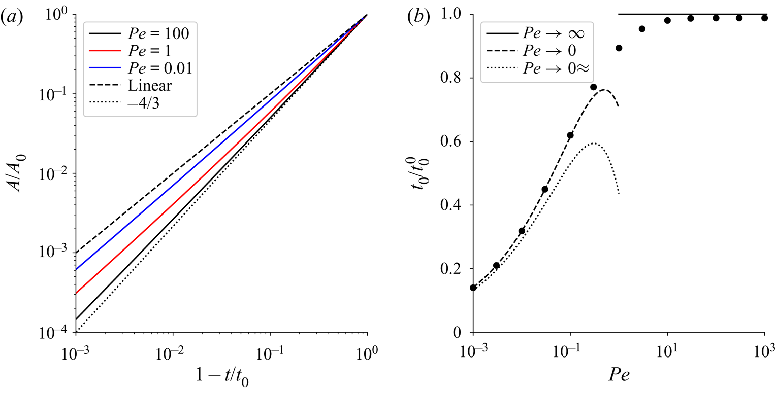
A log–log plot, shown in figure 10(a), indicates that the undissolved area is approximately a power of the time remaining before collapse  $A/A_0 = (1-t/t_0)^\alpha$. At high Péclet numbers
 $\alpha \approx 4/3$ as indicated in (4.8); however, contributions from Laurent coefficients with
 ${m < 0}$ modify the power, making it slightly less than
 $4/3$. Results at
 $Pe=100$ (solid black line) are asymptotic and show no discernible change at larger Péclet numbers. At lower Péclet numbers the exponents decrease towards a linear decay
 $A/A_0 = (1-t/t_0)$ (dotted line), which was predicted (Rycroft & Bazant Reference Rycroft and Bazant2016) from a low Péclet asymptotic expansion of the flux (§ 5.2). However, if the Péclet number is reduced below
 $Pe = 0.01$, there is only a minimal change from the blue line, suggesting that the predicted asymptotic limit, shown by the dotted line in figure 10(a), is never reached. Rycroft & Bazant (Reference Rycroft and Bazant2016) argued that the logarithmic term in
 $C$ could be assumed to be constant, but this approximation fails to capture the correct evolution of the area near the collapse point. In § 5.2 we developed an exact asymptotic (low
 $Pe$) calculation for the dissolution of an initially circular disk, which shows that there are logarithmic corrections to the linear decay that occurs for constant
 $C$.
Exact solutions for the time-dependent area (a) and collapse time (b). The  $x$ axis in panel (a) indicates the time remaining before collapse; note that time is decreasing in the positive direction. The areas are plotted logarithmically to show the approximate power-law scaling; the dashed line is the linear decay at low
 $Pe$ from Rycroft & Bazant (Reference Rycroft and Bazant2016), while the dotted line is the high
 $Pe$ asymptote
 $A(t)/A_0 = (1-t/t_0)^{4/3}$. The numerically determined collapse times are shown in panel (b) as a function of Péclet number. Asymptotic expressions for high and low Péclet numbers, from (4.9) and (5.15a,b), are shown as solid and dashed lines; the approximate low
 $Pe$ asymptote (5.11a,b) is shown as the dotted line.

The numerically determined collapse times  $t_0(Pe)$ are shown in figure 10(b). The collapse time is scaled by the high-
 $Pe$ asymptotic value
 $t_0^0 = \sqrt {Pe\,{\rm \pi} ^3/36}$. Since
 $t_0^0$ is an analytical approximation (4.9), it does not exactly capture the collapse time, even at large
 $Pe$, but is slightly too large; nevertheless, the collapse time at
 $Pe=100$ is within 1 % of
 $t_0^0$. At lower Péclet numbers the disk dissolves faster than predicted by the asymptotic flux (4.2), as indicated in figures 9(b) and 9(c). When
 $Pe < 1$ the disk remains circular (figure 9c), and all the Laurent coefficients apart from
 $a_1$ (radius) and
 $a_0$ (shift) are vanishingly small; an initially circular disk simply shrinks and shifts downstream (Rycroft & Bazant Reference Rycroft and Bazant2016). The exact low
 $Pe$ asymptote (§ 5.2) is indicated by the dashed line; the approximate asymptote assuming a constant
 $C = C(0)$ is shown as the dotted line.
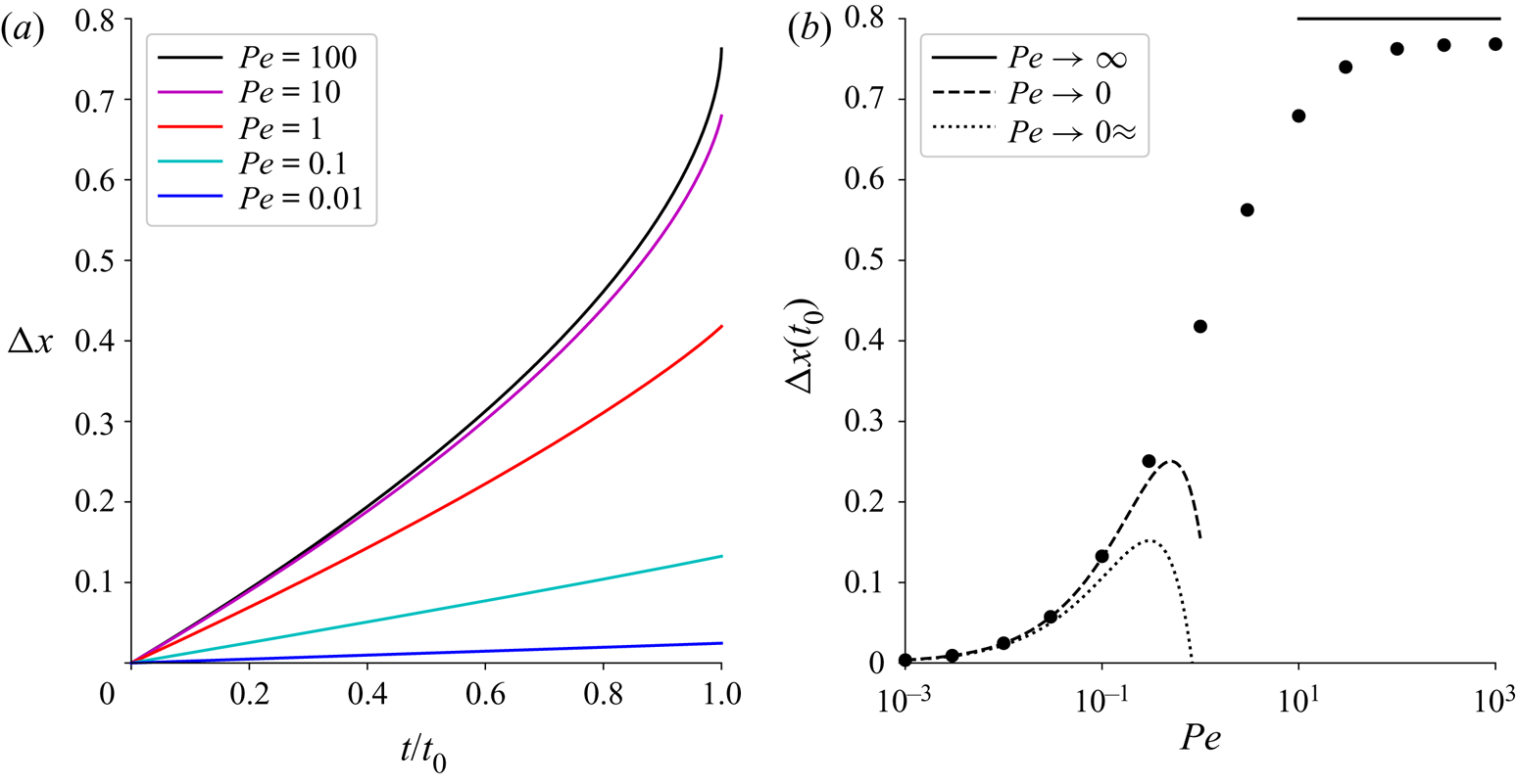
The centre of mass of the dissolving disk  ${\rm \Delta} x(t)$ is shown in figure 11 over a range of Péclet numbers. At low Péclet numbers the shift is nearly linear in time, but there are small logarithmic corrections (5.14), as discussed in § 5.2. At higher Péclet numbers the shift increases more rapidly with time and undergoes a sharp increase in slope near the collapse point. Nevertheless, there is a well-defined value for the shift at the collapse point
 ${\rm \Delta} x(t_0)$, which we have determined numerically as
 ${\rm \Delta} x(t_0, Pe\rightarrow \infty ) = 0.769$. The approximate value from (4.12a,b) is
 $0.800$, which is
 $4\,\%$ larger. The asymptotic approximations at high and low Péclet number are shown by the dashed lines in figure 11(b) and the approximate low
 $Pe$ shift at the collapse point (Rycroft & Bazant Reference Rycroft and Bazant2016) by the dotted line.
Exact solutions for the shift in centre of mass ( ${\rm \Delta} x$). (a) The time-dependent shift
 ${\rm \Delta} x(t)$ for different Péclet numbers. (b) The final shift
 ${\rm \Delta} x(t_0)$ versus Péclet number. Asymptotic expressions for high and low Péclet numbers, from (4.12a,b) and (5.14), are shown as solid and dashed lines; the approximate low
 $Pe$ asymptote from (5.11a,b) is shown as the dotted line.

The shape of the dissolving object can be characterized by the aspect ratio
 \begin{equation} A_R(t) = \frac{4A(t)}{{\rm \pi} L(t)^2} \end{equation}
where the area of the object  $A(t)$ is given in (3.19) and the length
 $L$ is the distance between the leading and trailing edges (4.14),
 \begin{equation} L(t) = S_0^{+}(t) - S_0^{-}(t) = 2\sideset{}{^\prime}\sum_{m=-M}^1 a_m(t), \end{equation}
here the sum is restricted to the odd coefficients  $a_1, a_{-1}, a_{-3}, \ldots$. For an elliptical object,
 $A_R$ is equal to the ratio of minor to major axes. The aspect ratio varies from one at
 $t=0$ (circular disk), to a smaller value at
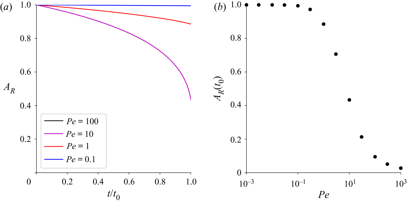
 $t_0$ (elliptical disk) resulting from the asymmetry introduced by the flow (figure 12a). For small Péclet numbers (
 $Pe < 0.1$) the aspect ratio remains constant, meaning that the disk is always circular. However, at
 $Pe = 1$ there is a growing asymmetry, not easily visible in figure 9(c), with
 $A_R \approx 0.9$ near the collapse point. At higher Péclet numbers the asymmetry becomes much larger, with a terminal aspect ratio
 $A_R(t_0) = 0.027$ at
 $Pe = 1000$ (figure 12b).
Exact solutions for the aspect ratio of the dissolving disk. (a) The time-dependent aspect ratio  $A_R(t)$ for different Péclet numbers. (b) The final aspect ratio
 $A_R(t_0)$ versus Péclet number.

5.4. The interplay of fluid velocity and conformal radius
The effective Péclet number  $Pe\,a_1(t)$ decreases with time as the solid dissolves, and eventually the dynamics is controlled by low
 $Pe$ asymptotics (Rycroft & Bazant Reference Rycroft and Bazant2016). Figure 13 shows the shapes of a dissolving cylinder at high initial Péclet number (
 $Pe=1000$). The surface coordinates have been scaled by the conformal radius
 $a_1$ so that the shapes near the collapse point remain visible; the coordinates are shifted along the
 $x$-axis to keep the centre of mass at the origin. The time
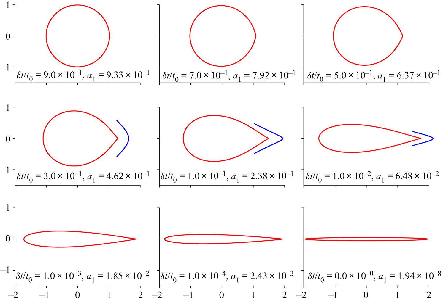
 $\delta t = t_0 - t$ indicates the time remaining before the solid vanishes.
Dissolution at different times to collapse,  $\delta t = t_0 - t$, for a Péclet number
 $Pe=1000$. Outlines of the shape of the undissolved solid (red lines) are scaled by the conformal radius (
 $a_1$), which is indicated in the legend. The blue lines show the region within 0.05 of the tip on a scale expanded sixteen fold. The inset plots (blue) have been shifted a small distance downstream to separate them from the main figures.

At high Péclet number ( $Pe=1000$) the disk develops a distinct cusp at the trailing edge, with slightly concave regions near the tip. By contrast, at lower Péclet numbers (figure 9) the trailing tip is always convex. However, although the tip looks sharp on the scale of the plot, an expanded scale shows that it remains slightly rounded (blue inset figures).
Starting with a high Péclet number means that the undissolved solid must be very small before the low- $Pe$ limit is approached. The collapse to the finite-time singularity (
 $\delta t \rightarrow 0$) is then very abrupt, as illustrated by the logarithmic time scale in the last row of figure 13. In high velocity erosion, an invariant triangular shape develops on the leading edge, which shrinks and shifts downstream with time (Moore et al. Reference Moore, Ristroph, Childress, Zhang and Shelley2013). Here, the shape of the solid body is evolving all the way to the end; there is no invariant shape.
Once  $Pe\,a_1$ drops below unity, all Laurent coefficients other than
 $a_1$,
 $a_0$, and
 $a_{-1}$ become small. The undissolved solid then takes up a roughly elliptical shape, which persists until collapse; the final shape can be seen in the last panel of figure 13. It may seem surprising in view of § 5.2 and figure 9(c) that the final shape is elliptical not circular. However, when the initial Péclet number is large, the object enters into the low
 $Pe$ asymptotic regime with a non-circular shape, so that the higher-order Laurent coefficients are decaying in time, but remain non-zero (Rycroft & Bazant Reference Rycroft and Bazant2016).
6. Conclusions
We have applied conformal-mapping methods to provide physical insight into the dissolution of thin cylinders of soluble materials such as gypsum. The approximations of potential flow and transport-limited dissolution, inherent in the application of conformal mapping, reduce the time scale by approximately 20 % and exaggerate the motion of the centre of mass. Nevertheless the predicted shapes are in remarkably good agreement with experimental observations (figure 1). Analysis of the Laurent coefficients that define the (time-dependent) map from the unit disk shows that the coefficients corresponding to the conformal radius ( $a_1$) and centre (
 $a_0$) largely separate from the negative indices (
 $a_{m<0}$) that specify the shape. It seems that the approximations separating (3.1)–(3.5a–c) from the experimental physics largely affect the conformal radius and centre, while leaving the negative Laurent coefficients almost unaffected. As the constraints – potential flow, diffusion-limited kinetics and an unbounded domain – are relaxed one by one, there are changes in both the time scale and location of the centre of mass, eventually leading to a very close match with experimental results.
We have solved the Polubarinova–Galin equation using different approximations for the flux of ions leaving the unit disk. For an exact solution at any Péclet number, we have implemented the integral equation formalism developed for frozen domains by Goldstein & Reid (Reference Goldstein and Reid1978) and Kornev & Mukhamadullina (Reference Kornev and Mukhamadullina1994). This extends previous asymptotic formulations (Bazant Reference Bazant2004; Rycroft & Bazant Reference Rycroft and Bazant2016) to the complete range of  $Pe$. At low Péclet numbers we have improved on previous work by including logarithmic corrections to the first three Laurent coefficients. There is then an exact match between numerical solutions and the low Péclet asymptotics, which compare well with the exact solutions when
 $Pe < 0.1$. The high Péclet asymptotic region begins around
 $Pe = 30$, and once again the area and shift in centre of mass can be found from simple analytical formulas for the first three Laurent coefficients, (4.8) and (4.12a,b). However, the high Péclet asymptotics is not entirely analytical because more coefficients are needed for a precise result; nevertheless, approximate results from the first three coefficients are frequently adequate.
The area of the dissolving body is linked to the evolution of the exterior harmonic moments in the  $z$ plane (Richardson Reference Richardson1972; Mineev-Weinstein, Wiegmann & Zabrodin Reference Mineev-Weinstein, Wiegmann and Zabrodin2000; Gustafsson & Vasil'ev Reference Gustafsson and Vasil'ev2006; Leshchiner et al. Reference Leshchiner, Thrasher, Mineev-Weinstein and Swinney2010), which can be defined as
 \begin{equation} B_m = \iint_{A_{ext}} z^{-m} \,\textrm{d} x \,\textrm{d} y - {\rm \pi}R_{ext}^2 \delta_{m,0} = -\frac{1}{2i}\oint_C z_b^{-m} \bar z_b \,\textrm{d} z_b, \end{equation}
where the exterior (fluid) domain  $A_{ext}$ is bounded by a large circle of radius
 $R_{ext}$,
 $m = 0, 1, 2, \ldots$ and
 $C$ is the boundary of the solid. The moments
 $B_m$ remain finite as
 $R_{ext} \rightarrow \infty$ and can be expressed as integrals over the unit circle,
 \begin{equation} B_m = -\tfrac{1}{2}\int_{-{\rm \pi}}^{\rm \pi} f^{-m}(\omega_b) \overline{f(\omega_b)} f^\prime(\omega_b) \omega_b \,\textrm{d}\theta. \end{equation}
The solid area  $A(t) = - B_0(t)$ can be directly connected to (3.19) by the equivalence of the two contour integrals (since
 $A(t)$ is real). For classical Laplacian growth (the
 $Pe \rightarrow 0$ limit of our system), a surprising result found by Richardson (Reference Richardson1972) is that
 $\dot B_m(t) = 0$ for
 $m>0$. In other words, all the harmonic moments are constant, except for the area itself. The infinite number of conservation laws links the evolution of the growing contour with the mathematics of integrable soliton systems (Mineev-Weinstein et al. Reference Mineev-Weinstein, Wiegmann and Zabrodin2000; Wiegmann & Zabrodin Reference Wiegmann and Zabrodin2000). The presence of the flow breaks the integrability, yet we observe a somewhat similar phenomenon, with the dynamics of the contour largely controlled by the first few terms.
Finally, we note that this work can be seen within the framework of a larger class of erosion and dissolution physics, both at high and low Reynolds numbers. Each regime gives rise to distinct shapes for the dissolving body.
(i) Erosion at large
$Re$: pointed leading edge, flat trailing edge (Ristroph et al. Reference Ristroph, Moore, Childress, Shelley and Zhang2012).(ii) Erosion at small
$Re$: pointed leading and trailing edges; symmetric shape (Quaife & Moore Reference Quaife and Moore2018).(iii) Dissolution at large
$Re$: rounded leading edge, flat trailing edge (Huang et al. Reference Huang, Moore and Ristroph2015).(iv) Dissolution at small
$Re$: rounded leading edge, pointed trailing edge (this work).


At high Reynolds number (cases i and iii), the boundary layer thickness scales as  $a_1^{1/2}$. The flux is proportional to
 $1/\delta$, which leads to the observed time dependence of the conformal radius (or size),
 $a_1(t) = (1-t/t_0)^{2/3}$. In case (iv) (this work), the concentration boundary layer again scales as
 $a_1^{1/2}$ because of the assumption of potential flow. However, in low
 $Re$ erosion (case ii), the area scaling is linear in time with logarithmic corrections (Quaife & Moore Reference Quaife and Moore2018). This is the same scaling observed in low Péclet dissolution (5.12).
Acknowledgements
Results from finite-volume simulations were generated with the OpenFOAM® toolkit (v.1706; http://www.openfoam.com/). Source codes used to calculate the evolution of the mapping functions are provided as a supporting file. Work at the University of Florida was supported by the U.S. Department of Energy, Office of Science, Office of Basic Energy Sciences, Chemical Sciences, Geosciences, and Biosciences Division under award number DE-SC0018676. Work at the University of Warsaw was supported by the National Science Centre (Poland) under research grant no. 2012/07/E/ST3/01734.
Declaration of interests
The authors report no conflict of interest.
Supplementary material
Supplementary material is available at https://doi.org/10.1017/jfm.2020.609.
Appendix A. Numerical solution for the flux around a disk
Here we outline a numerical solution of the integral equation from (5.5)
 \begin{equation} {\rm \pi}= \int_{0}^{\rm \pi} K\left[\lambda(\cos\theta-\cos\theta^\prime)\right]\sigma(\theta^\prime)\,\textrm{d} \theta^\prime, \end{equation}
where the kernel is given by
 \begin{equation} K(x) = \textrm{e}^x K_0(|x|), \end{equation}
and  $K_0$ is a modified Bessel function. The primary difficulty in integrating (A 1) is that the kernel has a logarithmic singularity in the region where
 $\theta \approx \theta ^\prime$. However, the (integrable) singularity can be eliminated by subtracting the source at the receiver point,
 \begin{equation} {\rm \pi}= \int_{0}^{\rm \pi} K\left[\lambda(\cos\theta-\cos\theta^\prime)\right] \left[\sigma(\theta^\prime) - \sigma(\theta) \right] \textrm{d} \theta^\prime + \sigma(\theta)\int_{0}^{\rm \pi} K\left[\lambda(\cos\theta-\cos\theta^\prime)\right] \textrm{d} \theta^\prime. \end{equation}
The first integral has a well-behaved integrand, vanishing as  $x \,\ln |x|$ in the region
 $\theta \approx \theta ^\prime$ (
 $x = \theta - \theta ^\prime$), and can be calculated by midpoint quadrature. We create a discrete set of
 $N$ points on the circle,
 $\theta _n = (n+\frac {1}{2}){\rm \pi} /N$, and calculate the off-diagonal matrix elements (
 $m\ne n$),
 \begin{equation} K_{mn} = \int_{\theta_n-\delta/2}^{\theta_n+\delta/2}K[\lambda(\cos\theta_m-\cos\theta^\prime)] \textrm{d}\theta^\prime = K\left[\lambda(\cos\theta_m-\cos\theta_n)\right] \delta, \end{equation}
with errors proportional to  $\delta ^3$, where
 $\delta = {\rm \pi}/N$.
We solve (A 3) for  $\sigma _m$ at each of the
 $N$ receiver points, which in the discrete representation becomes
 \begin{equation} \sum_{n=1}^N K_{mn} \sigma_n = {\rm \pi}, \end{equation}
with  $K_{m \ne n}$ given by (A 4), and
 \begin{equation} K_{mm} = I_m - \sum_{n \ne m} K_{mn}. \end{equation}
The integral  $I_m = \int _0^{\rm \pi} K[\lambda (\cos \theta _m-\cos \theta ^\prime )] \,\textrm {d} \theta ^\prime$ cannot be calculated by quadrature because of the singularity, so we must seek some kind of exact integration.
For a linear argument,  $K(a+bt)$, the kernel can be integrated exactly; in cases where
 $|a| > |bt|$,
 \begin{equation} \int \textrm{e}^{a+bt} K_0(|a+bt|) \,\textrm{d} t = \frac{a+bt}{b} \textrm{e}^{a+bt}\left(K_0 (|a+bt|) + \text{sgn}(a)K_1(|a+bt|)\right). \end{equation}
To make use of this result we subdivide the interval into  $2N_m+1$ subregions
 \begin{equation} \theta_n^k = \theta_n + k\delta^\prime, \end{equation}
where  $k = -N_m, -N_m+1, \ldots , N_m$ and
 $\delta ^\prime = \delta /(2N_m,+1)$
 \begin{equation} I_m = \sum_{n=1}^{N} \sum_{k=-N_m}^{N_m}\int_{-\delta^\prime/2}^{\delta^\prime/2}K \left[\lambda(\cos\theta_m-\cos(\theta_n^k + \theta^\prime))\right] \textrm{d}\theta^\prime. \end{equation}
If  $\delta ^\prime$ is sufficiently small, the argument of the kernel can be linearized about
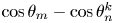 $\cos \theta _m-\cos \theta _n^k$,
 \begin{equation} I_m = \sum_{n=1}^N \sum_{k=-N_m}^{N_m} \int_{-\delta^\prime/2}^{\delta^\prime/2}K(a_m^{nk}+b^{nk}t)\,\textrm{d} t, \end{equation}
where  $a_m^{nk} = \lambda (\cos \theta _m - \cos \theta _n^k)$, and
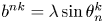 $b^{nk} = \lambda \sin \theta _n^k$. Typically, we set
 $N_m=8$ giving
 $17$ subintervals for each collocation point; increasing
 $N_m$ to 16 gave indistinguishable results. The integral over each segment can be evaluated exactly, but the formulas depend on the sign of
 $a_m^{nk}$, as in (A 7). Source codes to calculate these integrals are available in the supplementary material available at https://doi.org/10.1017/jfm.2020.609.