1 Introduction
Over the past decade, an important feature of global climate change has been the accelerating mass loss from the Antarctic and Greenland Ice Sheets (Rignot et al. Reference Rignot, Velicogna, van den Broeke, Monaghan and Lenaerts2011, Reference Rignot, Jacobs, Mouginot and Scheuchl2013). This mass loss is occurring on the underside and fronts of ice shelves formed where glaciers reach the polar oceans and from the icebergs that calve from them (Jenkins et al. Reference Jenkins, Dutrieux, McPhail, Perrett, Webb and White2010). Field observations of both icebergs and ice shelves indicate that this mass loss is an increasing function of ocean temperature (e.g. Budd, Jacka & Morgan Reference Budd, Jacka and Morgan1980; Shepherd, Wingham & Rignot Reference Shepherd, Wingham and Rignot2004).
Depending on the temperature of the seawater, icebergs and floating ice shelves may either melt or dissolve. Melting occurs when the seawater is sufficiently warm, and is controlled only by heat transfer (Woods Reference Woods1992; Kerr Reference Kerr1994a ). In contrast, dissolving occurs when the sea is close to or below the melting point of ice, and it is controlled by a combination of heat and mass transfer (Woods Reference Woods1992; Kerr Reference Kerr1994b ; Wells & Worster Reference Wells and Worster2011; Kerr & McConnochie Reference Kerr and McConnochie2015).
Previous studies have examined a horizontal ice face melting (Kerr Reference Kerr1994a
) or dissolving (Kerr Reference Kerr1994b
) into either overlying or underlying fluid as well as a sloping ice face melting in overlying fluid (Kerr Reference Kerr1994a
). The work of Kerr (Reference Kerr1994b
) has been extended for a vertical ice wall dissolving into cold, salty water by Kerr & McConnochie (Reference Kerr and McConnochie2015) who examined the interface temperature and composition, and the dissolution velocity. They found the dissolution velocity to depend on the
 $4/3$
power of the difference between the ocean temperature and its freezing point. They also found that the transition from dissolving to melting occurs at a temperature difference between the far-field fluid and the fluid at the interface of approximately
 $6\,^{\circ }\text{C}$
. In addition, insight can be gained from the complementary problem of solidification in various configurations (Huppert Reference Huppert1990).
In a geophysical context, ice faces are frequently sloping. In particular, the floating ice shelves seen at the edge of many Antarctic glaciers have very shallow basal slopes on large scales (e.g. Jenkins et al. Reference Jenkins, Dutrieux, McPhail, Perrett, Webb and White2010) but often contain steeper features on smaller scales (Dutrieux et al. Reference Dutrieux, Stewart, Jenkins, Nicholls, Corr, Rignot and Steffen2014). It is these small-scale features that this study aims to extend the results of Kerr & McConnochie (Reference Kerr and McConnochie2015) to, although there may be implications for melting on larger scales.
In this paper, we aim to quantify the turbulent dissolution of a sloping ice wall. In § 2, the theoretical model of dissolution presented in Kerr & McConnochie (Reference Kerr and McConnochie2015) is extended to the general case of a sloping ice face. In § 3, the model is compared with experimental observations of sloping ice faces dissolving in water at oceanic salinities. In § 4, we predict the turbulent convective dissolution of sloping ice bodies in the polar oceans. Our conclusions are presented in § 5.
2 Dissolving theory
In this section, we review turbulent thermal convection on vertical and sloping boundaries in § 2.1, before the dissolution of a sloping solid surface by turbulent compositional convection is considered in § 2.2.
2.1 Thermal convection
In understanding mass transfer due to turbulent compositional convection, very useful insight can be gained by examining the experimental measurements on heat transfer by natural convection tabulated by Holman (Reference Holman2010).
For laminar natural convection on an isothermal boundary of temperature
 $T_{w}$
facing downward at an angle
 $\unicode[STIX]{x1D703}$
to the vertical, the Nusselt number
 $Nu$
is given by
 $$\begin{eqnarray}\displaystyle & \displaystyle Nu\approx 0.56\,(Ra\cos \unicode[STIX]{x1D703})^{1/4} & \displaystyle\end{eqnarray}$$
(Holman Reference Holman2010, p. 344), where
 $Nu=qL(k(T_{w}-T_{f}))^{-1}$
,
 $q$
is the heat flux from the boundary,
 $L$
is the length of the boundary,
 $k$
is the thermal conductivity of the fluid,
 $T_{f}$
is the far-field temperature of the fluid,
 $Ra=g\unicode[STIX]{x1D6FC}(T_{w}-T_{f})L^{3}(\unicode[STIX]{x1D705}\unicode[STIX]{x1D708})^{-1}$
is the Rayleigh number,
 $g$
is the gravitational acceleration,
 $\unicode[STIX]{x1D6FC}$
is the thermal expansion coefficient of the fluid,
 $\unicode[STIX]{x1D705}$
is the thermal diffusivity of the fluid, and
 $\unicode[STIX]{x1D708}$
is the kinematic viscosity of the fluid. Equation (2.1) was measured in water by Fujii & Imura (Reference Fujii and Imura1972) for values of
 $\unicode[STIX]{x1D703}$
from
 $0^{\circ }$
to
 $86.8^{\circ }$
and values of
 $Ra\cos \unicode[STIX]{x1D703}$
from
 $10^{5}$
to
 $10^{11}$
. In (2.1), the heat transfer is seen to depend on the component of gravitational acceleration up the sloping boundary,
 $g\cos \unicode[STIX]{x1D703}$
.
For turbulent natural convection on a constant heat flux boundary facing downward at an angle
 $\unicode[STIX]{x1D703}$
, the Nusselt number at high flux Rayleigh numbers
 $Ra_{f}$
is empirically correlated by
 $$\begin{eqnarray}\displaystyle & \displaystyle Nu\approx 0.17\,(Ra_{f}\cos ^{2}\unicode[STIX]{x1D703})^{1/4} & \displaystyle\end{eqnarray}$$
(Holman Reference Holman2010, p. 345), where
 $Ra_{f}=g\unicode[STIX]{x1D6FC}qL^{4}(k\unicode[STIX]{x1D705}\unicode[STIX]{x1D708})^{-1}$
. Equation (2.2) was measured in air by Vliet & Ross (Reference Vliet and Ross1975) for values of
 $\unicode[STIX]{x1D703}$
from
 $0^{\circ }$
to
 $80^{\circ }$
and values of
 $Ra_{f}\cos ^{2}\unicode[STIX]{x1D703}$
that ranged from
 $10^{10}$
to
 $10^{15}$
. Vliet & Ross (Reference Vliet and Ross1975) attributed the dependence of the heat transfer on the angle
 $\unicode[STIX]{x1D703}$
to a combination of the component of gravitational acceleration up the sloping boundary, and ‘the damping of the turbulence due to the thermally stable condition of the boundary layer flow’.
Since
 $Ra_{f}=Ra\,Nu$
, (2.2) is equivalent to
 $$\begin{eqnarray}\displaystyle & \displaystyle Nu\approx (0.17)^{4/3}Ra^{1/3}\cos ^{2/3}\unicode[STIX]{x1D703}=0.094\,Ra^{1/3}\cos ^{2/3}\unicode[STIX]{x1D703}. & \displaystyle\end{eqnarray}$$
It is important to note that the one-third power law dependence in (2.3) implies that the turbulent heat flux is independent of the length of the boundary and independent of position on the boundary (Holman Reference Holman2010, p. 337).
By assuming that the heat transport is continuous across the laminar–turbulent transition we can combine (2.1) and (2.3) to give a critical Rayleigh number where the transition will occur:
 $$\begin{eqnarray}\displaystyle & \displaystyle Ra_{c}\sim {\displaystyle \frac{2.0\times 10^{9}}{\cos ^{5}\unicode[STIX]{x1D703}}}. & \displaystyle\end{eqnarray}$$
This critical Rayleigh number corresponds to a critical transition distance up the sloping boundary of
 $$\begin{eqnarray}\displaystyle & \displaystyle L_{c}\sim {\displaystyle \frac{1260}{\cos ^{5/3}\unicode[STIX]{x1D703}}}\left({\displaystyle \frac{\unicode[STIX]{x1D705}\unicode[STIX]{x1D708}}{g\unicode[STIX]{x1D6FC}(T_{w}-T_{f})}}\right)^{1/3}. & \displaystyle\end{eqnarray}$$
It is noted that this distance is measured in the wall-parallel direction and is not the vertical height.
2.2 Dissolution of a sloping solid surface by turbulent compositional convection
Kerr & McConnochie (Reference Kerr and McConnochie2015) presented a theoretical analysis that predicted the ablation velocity and interface conditions of a dissolving vertical solid surface based on empirical heat transfer relationships equivalent to (2.3). The model was itself an extension of previous work investigating a horizontal surface dissolving into fluid above it (Kerr Reference Kerr1994b ).
The model envisages thermal and compositional boundary layers that grow diffusively until a time
 $\unicode[STIX]{x1D70F}$
when they are periodically removed by the eddies associated with turbulent compositional convection (cf. Lick Reference Lick1965; Howard Reference Howard and Görtler1966). The model can be generalised for a surface that is facing downward at an angle
 $\unicode[STIX]{x1D703}$
to the vertical by including the angle dependence that is given in (2.3).
We consider a solid surface with composition
 $C_{s}$
and far-field temperature
 $T_{s}$
in contact with a semi-infinite fluid with a far-field composition
 $C_{f}$
and far-field temperature
 $T_{f}$
. There are three unknown quantities at the interface between the solid and the fluid: the interface temperature
 $T_{i}$
, interface composition
 $C_{i}$
and the dissolution velocity
 $V$
. The analysis of Kerr & McConnochie (Reference Kerr and McConnochie2015), together with the heat transfer relationship given in (2.3), result in
 $T_{f}-T_{i}$
and the velocity scale
 ${\mathcal{V}}$
being given by
 $$\begin{eqnarray}\displaystyle & \displaystyle T_{f}-T_{i}={\displaystyle \frac{\unicode[STIX]{x1D70C}_{s}L_{s}+\unicode[STIX]{x1D70C}_{s}c_{s}(T_{i}-T_{s})}{\unicode[STIX]{x1D70C}_{f}c_{f}}}\,\left({\displaystyle \frac{D}{\unicode[STIX]{x1D705}_{f}}}\right)^{1/2}\left({\displaystyle \frac{C_{f}-C_{i}}{C_{f}-C_{s}}}\right) & \displaystyle\end{eqnarray}$$
and
 $$\begin{eqnarray}\displaystyle & \displaystyle {\mathcal{V}}={\displaystyle \frac{V}{\unicode[STIX]{x1D6FE}}}=\cos ^{2/3}\unicode[STIX]{x1D703}\,\left({\displaystyle \frac{g(\unicode[STIX]{x1D70C}_{f}-\unicode[STIX]{x1D70C}_{i})D^{2}}{\unicode[STIX]{x1D707}}}\right)^{1/3}\left({\displaystyle \frac{C_{f}-C_{i}}{C_{f}-C_{s}}}\right), & \displaystyle\end{eqnarray}$$
where subscript
 $f$
corresponds to fluid properties, subscript
 $i$
corresponds to properties at the interface, subscript
 $s$
corresponds to solid properties,
 $\unicode[STIX]{x1D70C}$
is the density,
 $L$
is the latent heat of fusion,
 $c$
is the specific heat,
 $D$
is the compositional diffusivity and
 $\unicode[STIX]{x1D707}$
is the fluid dynamic viscosity.
 $\unicode[STIX]{x1D6FE}$
is a constant of proportionality equal to approximately 0.094 (from (2.3)) or
 $0.090\pm 0.004$
(from Kerr & McConnochie (Reference Kerr and McConnochie2015)).
Equations (2.6) and (2.7) can be solved for the three unknowns using the thermodynamic constraint that the interface temperature and salinity must lie on the liquidus curve. However, from inspection it can be seen that the angle
 $\unicode[STIX]{x1D703}$
is predicted to have no effect on the interface conditions, while the dissolution velocity is predicted to be proportional to
 $\cos ^{2/3}\unicode[STIX]{x1D703}$
.
A correction for the moving solid–liquid boundary has been applied which results in (2.6) and (2.7) being valid when
 $(C_{f}-C_{i})\approx (C_{i}-C_{s})$
. This correction increases the compositional boundary layer thickness to account for the fact that the interface will retreat as the boundary layer grows. As a result, the compositional boundary layer thickness
 $h_{c}$
is more accurately given by
 $\sqrt{D\unicode[STIX]{x1D70F}}+V\unicode[STIX]{x1D70F}$
than by
 $\sqrt{D\unicode[STIX]{x1D70F}}$
. When
 $(C_{f}-C_{i})\ll (C_{i}-C_{s})$
the velocity of the boundary is negligible and the final term in (2.6) and (2.7) should be replaced with
 $(C_{f}-C_{i})/(C_{i}-C_{s})$
. Furthermore, when
 $(C_{f}-C_{i})\gg (C_{i}-C_{s})$
the model breaks down as the turbulent dissolution undergoes a transition to turbulent melting (see appendix of Kerr (Reference Kerr1994b
)).
The model also assumes that the compositional buoyancy released at the interface dominates the thermal buoyancy. As in Kerr & McConnochie (Reference Kerr and McConnochie2015), this condition can be described based on the ratio of compositional to thermal buoyancy
 ${\mathcal{R}}$
as:
 $$\begin{eqnarray}\displaystyle & \displaystyle {\mathcal{R}}={\displaystyle \frac{\unicode[STIX]{x1D6FD}(C_{f}-C_{s})\unicode[STIX]{x1D70C}_{f}c_{f}}{\unicode[STIX]{x1D6FC}[\unicode[STIX]{x1D70C}_{s}L_{s}+\unicode[STIX]{x1D70C}_{s}c_{s}(T_{i}-T_{s})]}}\gg 1, & \displaystyle\end{eqnarray}$$
where
 $\unicode[STIX]{x1D6FD}$
is the compositional expansion coefficient. This condition is generally met in the polar oceans as
 $\unicode[STIX]{x1D6FC}$
approaches zero at low temperatures.
When considering compositional convection, (2.5) needs to be adjusted to reflect properties of the solute rather than then thermal field. As such, (2.5) should be rewritten as:
 $$\begin{eqnarray}\displaystyle & \displaystyle L_{c}\sim {\displaystyle \frac{1260}{\cos ^{5/3}\unicode[STIX]{x1D703}}}\left({\displaystyle \frac{D\unicode[STIX]{x1D708}}{g\unicode[STIX]{x1D6FD}(C_{i}-C_{f})}}\right)^{1/3}. & \displaystyle\end{eqnarray}$$
For a vertical ice wall dissolving into the polar oceans at temperatures from
 $-1$
to
 $5\,^{\circ }\text{C}$
, using values of the physical constants and interface conditions from Kerr & McConnochie (Reference Kerr and McConnochie2015), equation (2.9) suggests that the compositional boundary layer undergoes a transition from laminar to turbulent flow at a distance from the base
 $L_{c}$
of 2–4 cm. In comparison, laboratory experiments using vertical ice walls have found that the transition to turbulence actually occurs at heights of 10–30 cm (Josberger & Martin Reference Josberger and Martin1981; Carey & Gebhart Reference Carey and Gebhart1982; Johnson & Mollendorf Reference Johnson and Mollendorf1984; Kerr & McConnochie Reference Kerr and McConnochie2015).
A possible explanation of this discrepancy lies in the observation of bidirectional flow in the laminar region next to a dissolving ice face (Josberger & Martin Reference Josberger and Martin1981). Due to the higher molecular diffusivity of heat than salt, the thermal boundary layer is significantly thicker than the haline boundary layer. In the laminar region this leads to a rising haline boundary layer close to the wall and a sinking thermal boundary layer further away from the wall. Once the flow is turbulent the two boundary layers are relatively well mixed and the boundary layer is one-directional. The interaction between the two boundary layers in the laminar region could have an important impact on the laminar–turbulent transition that is not included in the previous thermal experiments that were used to derive (2.5).
3 Comparison with laboratory experiments
To test (2.6), (2.7) and (2.9) we have conducted a series of experiments with a sloping ice face dissolving into cold salty water. The values that were used for the physical constants in (2.6), (2.7) and (2.9) are given in table 2 of Kerr & McConnochie (Reference Kerr and McConnochie2015). The experiments were performed in a temperature controlled room set at approximately
 $4\,^{\circ }\text{C}$
in a rectangular tank that was 1.2 m high, 0.2 m wide and 1.5 m long. A detailed description of the apparatus and experimental procedure are given in Kerr & McConnochie (Reference Kerr and McConnochie2015).
Within the tank was an aluminium heat exchanger that could be rotated to give a range of slopes. The ice was grown from fresh water against the sloping heat exchanger before the fluid was drained and replaced with salt water. The temperature and salinity of the far-field fluid was kept at approximately
 $4.5\,^{\circ }\text{C}$
(
 $3.7{-}5.7\,^{\circ }\text{C}$
) and 3.5 wt % NaCl (
 $3.46{-}3.64~\text{wt}\,\%$
NaCl) respectively. The slope angle was varied in the range
 $20{-}39.5^{\circ }$
from the vertical, in addition to a case where the slope angle was
 $0^{\circ }$
. Slopes between
 $0^{\circ }$
and
 $20^{\circ }$
were not performed as
 $\cos \unicode[STIX]{x1D703}$
changes by only a small amount within this range. Slopes shallower than
 $39.5^{\circ }$
were unfortunately not possible due to the turbulent transition length increasing as
 $\cos ^{-5/3}\unicode[STIX]{x1D703}$
(see (2.9)). Further increasing the slope would have resulted in laminar flow over too great an extent of the tank, resulting in the measurements being unreliable or impossible.
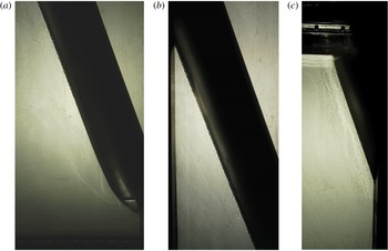
Figure 1 shows a photo from a typical experiment. The flow is visualised with the shadowgraph method. This particular experiment had a far-field temperature of
 $3.9\,^{\circ }\text{C}$
, a far-field salinity of 3.56 wt % NaCl, and a slope angle of
 $20^{\circ }$
. The white patches that are visible to the left of the ice are due to reflection off the ice face.
Shadowgraph images of the turbulent boundary layer flowing up the ice wall after approximately 20 min of an experiment with
 $T_{f}=3.9\,^{\circ }\text{C}$
,
 $C_{f}=3.56~\text{wt}\,\%$
NaCl and
 $\unicode[STIX]{x1D703}=20^{\circ }$
. (a) Shows the base of the tank to a height of 46 cm, (b) shows a height of 34–81 cm and (c) shows a height of 75 cm to the top of the fluid at 112 cm. The sloping dark object in each image is the heat exchanger and ice face. The vertical dark object in (b) and (c) is a support brace that sits on the outside of the tank. The transition to turbulence can be seen in (a).

Measurements of the ablation velocity and interface temperature were made throughout an experiment as described by Kerr & McConnochie (Reference Kerr and McConnochie2015). The uncertainty in interface temperature is estimated to be
 $0.1\,^{\circ }\text{C}$
based on measurements from thermistors frozen at the same height (Kerr & McConnochie Reference Kerr and McConnochie2015) while the uncertainty in ablation velocity is calculated by comparing our experimental results with (2.7). In addition to measuring the interface temperature and ablation velocity, the laminar–turbulent transition length
 $L_{c}$
was measured based on the shadowgraph imagery.
Measurements of the transition length were made from visual inspection of the flow and contain significant uncertainty. Particularly for shallow slope angles, pulses of turbulence began occurring over a range of heights. For each experiment the minimum and maximum height where turbulent eddies began to form was recorded and the average of these values is reported as the transition length.
A further complication when measuring the transition length was the fact that the bottom 5 cm of the ice was not planar. Instead, the ice curved around the base of the heat exchanger, increasing the slope angle near the bottom of the tank. The uncertainty associated with this will be largest for steep angles where the transition length is smallest but is not expected to be significant. Despite the uncertainty in measurements of the transition length, the results are sufficient to test the dependence on slope angle predicted by (2.9).
3.1 Ablation velocity
Equation (2.7) predicts that the ablation velocity will scale with
 $\cos ^{2/3}\unicode[STIX]{x1D703}$
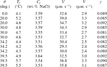
. Table 1 gives the experimental conditions and results used to test this prediction and to evaluate the constant of proportionality
 $\unicode[STIX]{x1D6FE}$
.
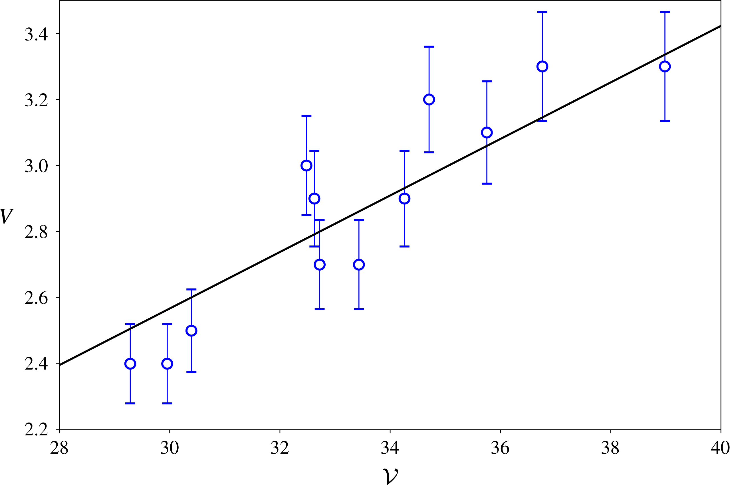
The measured ablation velocity as a function of the velocity scale given in (2.7). The straight line gives the predicted ablation velocity with
 $\unicode[STIX]{x1D6FE}=0.086$
. The error bars show the estimated experimental uncertainty of
 $\pm 5\,\%$
based on repeated experiments.

Measured ablation velocities
 $V$
with the experimental slope angle, far-field temperature
 $T_{f}$
, far-field salinity
 $C_{f}$
, the velocity scale from (2.7)
 ${\mathcal{V}}$
and calculated values of
 $\unicode[STIX]{x1D6FE}$
. The average value of
 $\unicode[STIX]{x1D6FE}$
across all experiments is 0.086.

The constant of proportionality
 $\unicode[STIX]{x1D6FE}$
is evaluated to be approximately
 $0.086\pm 0.005$
based on the experimental data given in table 1. This is slightly lower but comparable to the equivalent constant for a vertical ice wall reported by Kerr & McConnochie (Reference Kerr and McConnochie2015) of
 $0.090\pm 0.004$
. There is no systematic variation of
 $\unicode[STIX]{x1D6FE}$
with
 $\unicode[STIX]{x1D703}$
suggesting that the difference is due to experimental uncertainty rather than any further dependence on
 $\unicode[STIX]{x1D703}$
.
Figure 2 shows the measured ablation velocity
 $V$
plotted against the velocity scale
 ${\mathcal{V}}$
. The average value of
 $\unicode[STIX]{x1D6FE}$
from the experiments given in table 1 is used to plot the predicted ablation velocity (black line). The experimental measurements agree with the predicted ablation velocity to within the experimental uncertainty which is primarily due to the resolution of the photographs used to make the measurements.
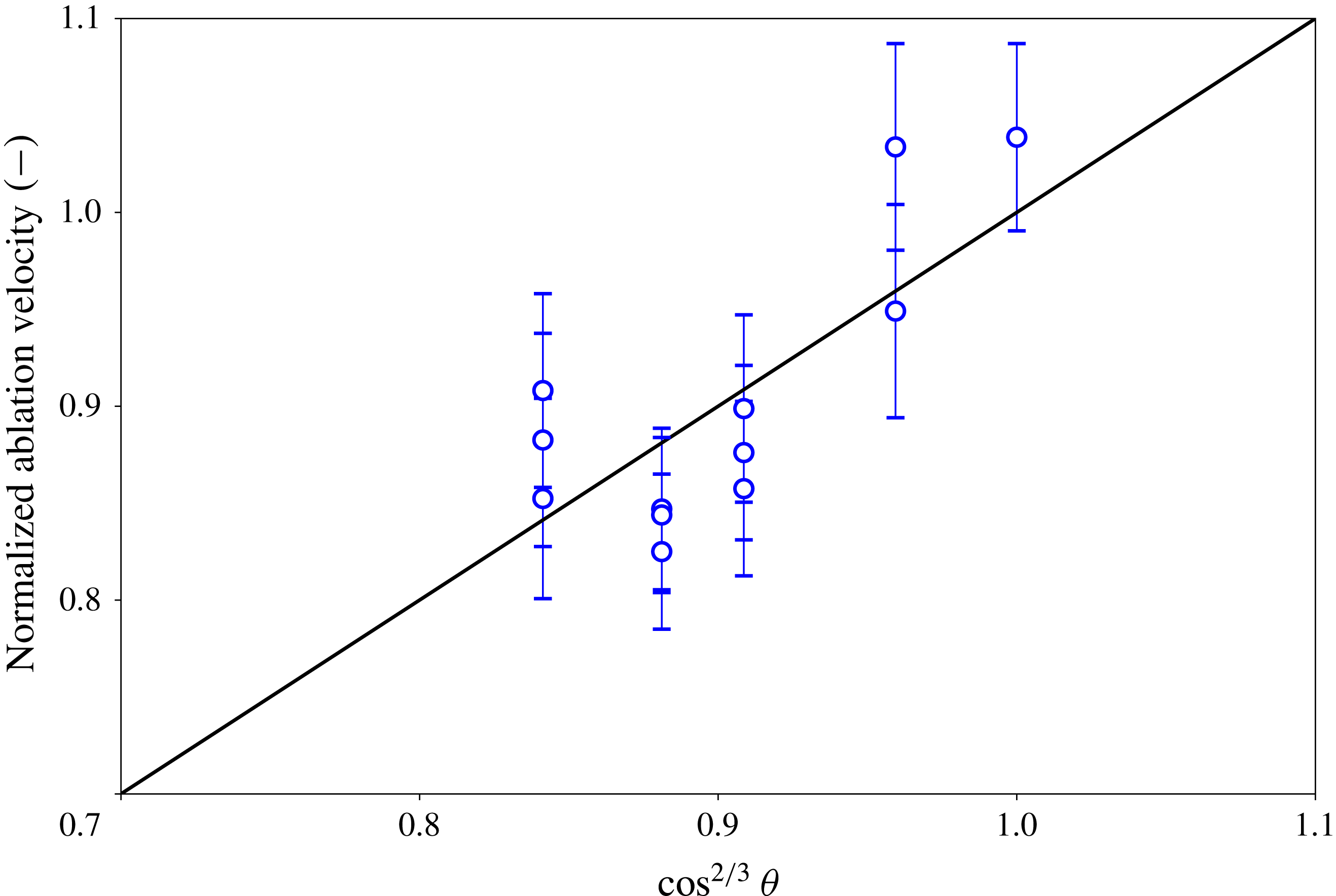
To remove any potential effects of the far-field conditions the ablation velocity has been normalised by the expected ablation velocity under the same ambient fluid conditions but a vertical ice wall. This normalised ablation velocity is plotted in figure 3.
The normalised ablation velocity as a function of
 $\cos ^{2/3}\unicode[STIX]{x1D703}$
. The ablation velocity has been normalised by the predicted ablation velocity given the same far-field conditions but a vertical wall. The error bars show the estimated experimental uncertainty of
 $\pm 5\,\%$
based on repeated experiments.

3.2 Interface temperature
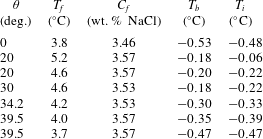
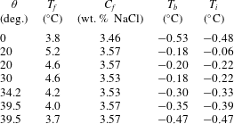
Table 2 gives the measured (
 $T_{b}$
) and predicted (
 $T_{i}$
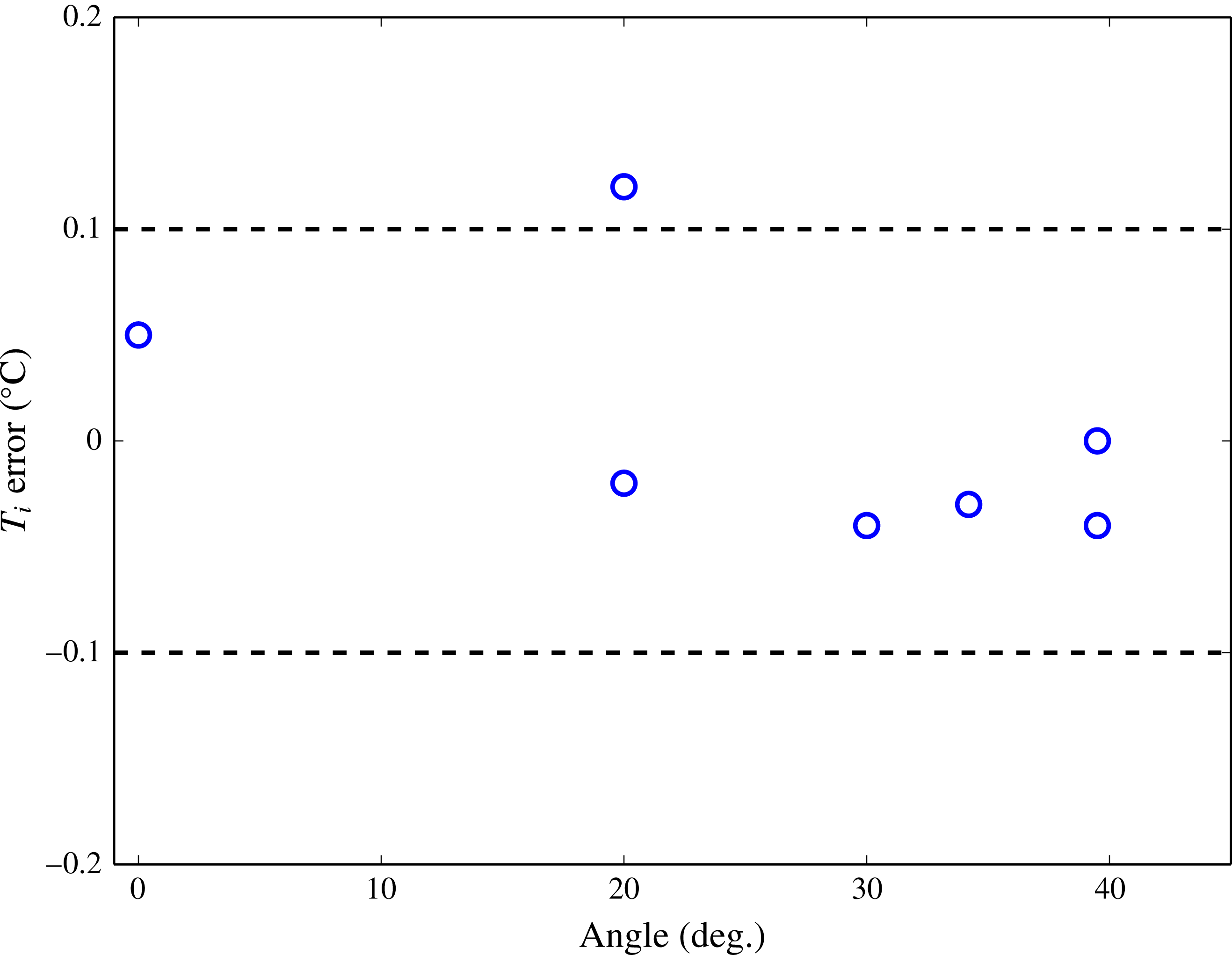
) interface temperatures with the far-field conditions and slope angle. Figure 4 shows the difference between the predicted and measured interface temperatures as a function of angle
 $\unicode[STIX]{x1D703}$
. The values for
 $\unicode[STIX]{x1D703}=0^{\circ }$
are taken from experiment E of Kerr & McConnochie (Reference Kerr and McConnochie2015).
Measured (
 $T_{b}$
) and predicted (
 $T_{i}$
) interface temperatures with the experimental slope angle
 $\unicode[STIX]{x1D703}$
, far-field temperature
 $T_{f}$
and far-field salinity
 $C_{f}$
. The values for
 $\unicode[STIX]{x1D703}=0^{\circ }$
are taken from experiment E of Kerr & McConnochie (Reference Kerr and McConnochie2015).
Difference between the experimental and predicted interface temperature as a function of slope angle
 $\unicode[STIX]{x1D703}$
. The two dashed lines show the expected
 $0.1\,^{\circ }\text{C}$
experimental uncertainty based on previous experiments (Kerr & McConnochie Reference Kerr and McConnochie2015). The value for
 $\unicode[STIX]{x1D703}=0^{\circ }$
is the average difference between the measured and predicted interface temperature from the experiments of Kerr & McConnochie (Reference Kerr and McConnochie2015).

Based on previous experiments (Kerr & McConnochie Reference Kerr and McConnochie2015), we estimate the uncertainty in measurements of the interface temperature to be approximately
 $0.1\,^{\circ }\text{C}$
. This experimental uncertainty is shown by the dashed lines in figure 4. The difference between our experimental interface temperatures and that predicted by (2.6) is generally less than the experimental uncertainty, suggesting that (2.6) is able to accurately predict the interface temperature over a range of slopes.
The experimental results and (2.6) show that the interface temperature is independent of the slope angle
 $\unicode[STIX]{x1D703}$
. The interface temperature depends on the relative transport of heat and salt to the interface which is primarily controlled by the ratio of the thermal and haline diffusivity. Given that these physical quantities are unaffected by the geometry of the ice face, it is unsurprising that the interface temperature is also unaffected by the geometry of the ice.
3.3 Transition length
Finally, the experimental results are used to test (2.9). As noted in § 2.1, the theoretical transition length is smaller than that which is observed in the case of a vertical ice wall dissolving into salt water. This discrepancy could be due to the instability being suppressed by the bidirectional flow caused by the opposing buoyancy of the temperature and salinity fields (Josberger & Martin Reference Josberger and Martin1981). Such an effect cannot occur in the thermal experiments used to derive (2.9) as the boundary layer flow is purely one-directional. When comparing our experimental measurements of the transition length to (2.9) we have used a non-dimensionalised length scale defined as
 $$\begin{eqnarray}\displaystyle & \displaystyle L_{c}^{\ast }=L_{c}\,\left({\displaystyle \frac{g(\unicode[STIX]{x1D70C}_{f}-\unicode[STIX]{x1D70C}_{i})}{D\unicode[STIX]{x1D707}}}\right)^{1/3}. & \displaystyle\end{eqnarray}$$
The term
 $(g(\unicode[STIX]{x1D70C}_{f}-\unicode[STIX]{x1D70C}_{i})/(D\unicode[STIX]{x1D707}))^{1/3}$
is approximately equal to
 $56\,000~\text{m}^{-1}$
for our experiments but varies slightly due to different far-field conditions. From (2.9) we expect
 $L_{c}^{\ast }=A\,\cos ^{-5/3}\unicode[STIX]{x1D703}$
where the coefficient
 $A$
will be determined from the experimental results.
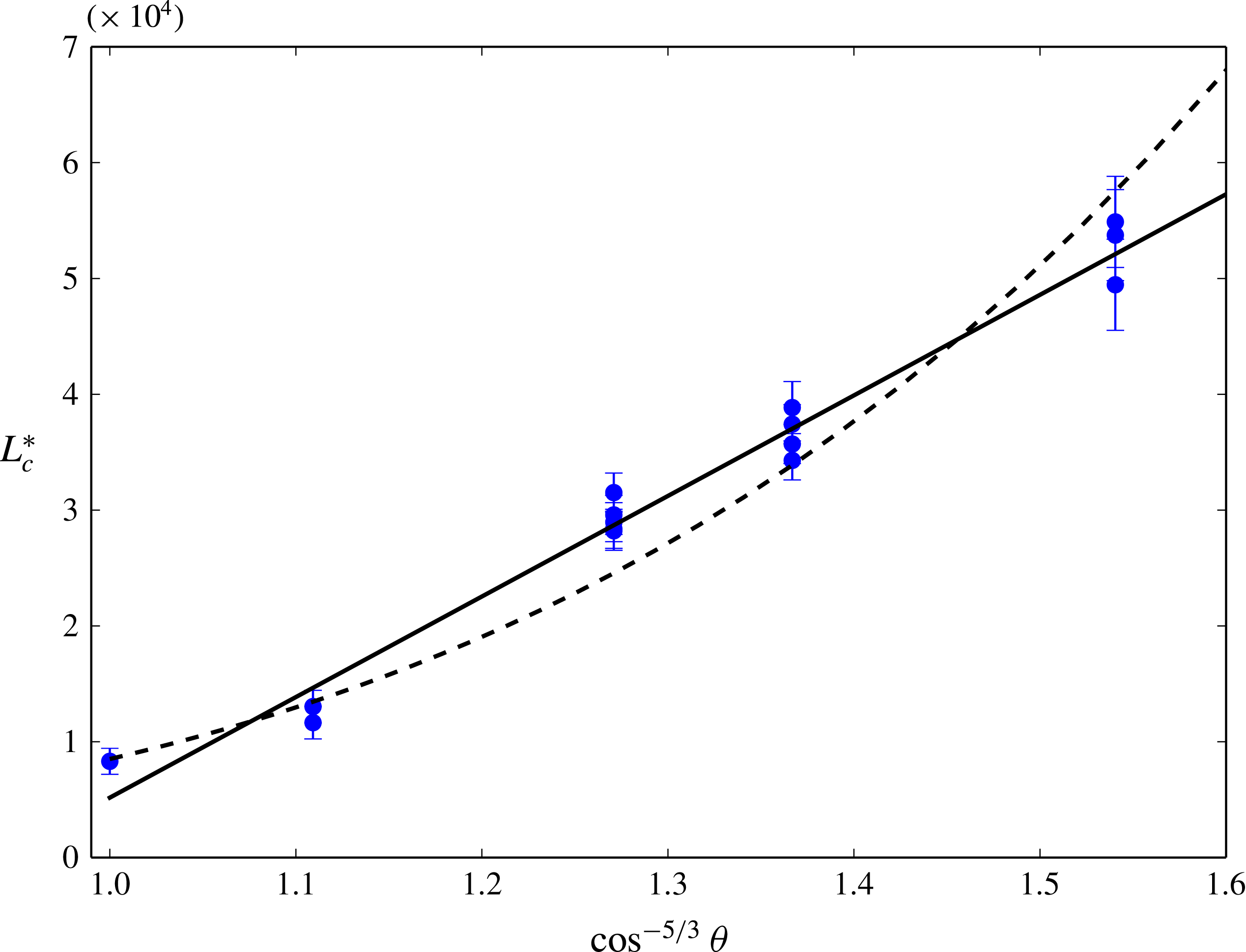
Experimental values of the non-dimensional transition length plotted against
 $\cos ^{-5/3}\unicode[STIX]{x1D703}$
. The solid line shows
 $L_{c}^{\ast }=86\,840\,\cos ^{-5/3}\unicode[STIX]{x1D703}\,-81\,670$
and the dashed line shows
 $L_{c}^{\ast }=8506\,\cos ^{-7.37}\unicode[STIX]{x1D703}$
.

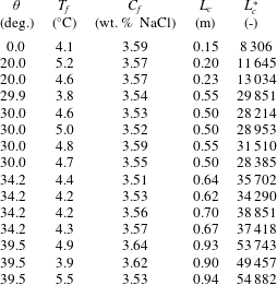
Measured transition length
 $L_{c}$
with the experimental slope angle
 $\unicode[STIX]{x1D703}$
, far-field temperature
 $T_{f}$
, far-field salinity
 $C_{f}$
and the non-dimensionalised transition length
 $L_{c}^{\ast }$
, from (3.1).
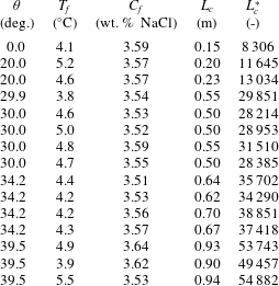
Table 3 gives the dimensional and non-dimensionalised transition lengths with the experimental conditions for each experiment. Figure 5 shows the non-dimensional transition length plotted against
 $\cos ^{-5/3}\unicode[STIX]{x1D703}$
. The error bars shown in figure 5 indicate the range of locations where turbulent fluctuations first appeared. When the slope is steep the onset of turbulent fluctuations was visually obvious and consistent in time. However, for shallow slope angles, pulses of turbulence originated over a wide range of heights and grew less rapidly.
The solid line in figure 5 shows
 $L_{c}^{\ast }=86\,840\,\cos ^{-5/3}\unicode[STIX]{x1D703}\,-81\,671$
. In order for
 $L_{c}\sim \cos ^{-5/3}\unicode[STIX]{x1D703}$
, as predicted by (2.9), a significant offset needs to be added to the equation. The dashed line shows
 $L_{c}^{\ast }=8506\,\cos ^{-7.37}\unicode[STIX]{x1D703}$
. This was obtained from fitting a power law to the experimental data.
Figure 5 suggests that, within our experimental parameters, the non-dimensional transition length can be given by
 $$\begin{eqnarray}\displaystyle & \displaystyle L_{c}^{\ast }=86\,840\,\cos ^{-5/3}\unicode[STIX]{x1D703}\,-81\,671 & \displaystyle\end{eqnarray}$$
or
 $$\begin{eqnarray}\displaystyle & \displaystyle L_{c}^{\ast }=8506\,\cos ^{-7.37}\unicode[STIX]{x1D703}. & \displaystyle\end{eqnarray}$$
The difference between the two power laws given in (3.2) and (3.3) is significant. For example, at similar far-field conditions to our experiments and a slope angle of
 $\unicode[STIX]{x1D703}=60^{\circ }$
, equation (3.2) would predict a transition length of 3.4 m while (3.3) would predict a transition length of 25 m. Without measurements of the transition length at shallower slope angles it is difficult to assess which power law is more accurate. If (3.3) is valid, then the presence of both salinity and temperature boundary layers greatly enhances the sensitivity of slope angle on the transition length compared to what was predicted by (2.9).
4 Ice shelf dissolution in seawater
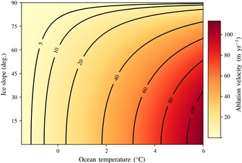
Here we apply the theory presented in § 2.2 to geophysical ice shelves. Equation (2.7) is used to calculate the ablation velocity as a function of ocean temperature and basal slope. The results are shown on figure 6. The interior of the ice is assumed to have a temperature
 $T_{s}$
of
 $-25\,^{\circ }\text{C}$
(Holland & Jenkins Reference Holland and Jenkins1999) and zero salinity while the ocean salinity is assumed to be
 $35~\text{g}~\text{kg}^{-1}$
. The density, specific heat, latent heat and freezing point are obtained from the thermodynamic equation of seawater (IOC, SCOR & IAPSO 2010), the fluid thermal conductivity and viscosity are obtained from Sharqawy, Lienhard & Zubair (Reference Sharqawy, Lienhard and Zubair2010) and the compositional diffusivity of NaCl is used (Kerr & McConnochie Reference Kerr and McConnochie2015). The value of
 $\unicode[STIX]{x1D6FE}$
is taken from the experimental results to be 0.086. The calculations are based on fluid at the surface but can be approximated for any depth by adding the freezing point depression due to pressure to the in situ ocean temperature.
On large scales, the basal slopes of Antarctic ice shelves are much shallower than those produced in our experiments (
 ${\approx}87^{\circ }$
). However, high resolution observations underneath the Pine Island Glacier ice shelf and Petermann Glacier, Greenland suggest that the basal topography is broken into a series of near-horizontal sections separated by sharp changes in elevation (Dutrieux et al.
Reference Dutrieux, Stewart, Jenkins, Nicholls, Corr, Rignot and Steffen2014). It is these relatively steep features that we will focus on as they are most applicable to the laboratory experiments.
Calculated values of the ablation velocity for ice in seawater as a function of ocean temperature and basal slope. The basal slope is measured from the vertical for consistency with the experiments and (2.7).

Meltwater channels have been observed under the Pine Island Glacier ice shelf and Petermann Glacier (Dutrieux et al.
Reference Dutrieux, Stewart, Jenkins, Nicholls, Corr, Rignot and Steffen2014). These channels are arranged both parallel and perpendicular to the glacier flow. The channels are approximately 200 m wide at the base and 200 m high, suggesting an average slope angle of approximately
 $27^{\circ }$
from the vertical. Considering the Petermann Glacier, we use an ocean temperature of
 $0.15\,^{\circ }\text{C}$
and a basal depth of 400 m (Dutrieux et al.
Reference Dutrieux, Stewart, Jenkins, Nicholls, Corr, Rignot and Steffen2014) to calculate a predicted melt rate of
 $17.0~\text{m}~\text{yr}^{-1}$
. This is very similar to the
 ${\sim}15~\text{m}~\text{yr}^{-1}$
that was measured on the channel flank by Dutrieux et al. (Reference Dutrieux, Stewart, Jenkins, Nicholls, Corr, Rignot and Steffen2014).
Under Pine Island Glacier ice shelf, Dutrieux et al. (Reference Dutrieux, Stewart, Jenkins, Nicholls, Corr, Rignot and Steffen2014) also observed a series of terraces separated by steep walls. The terraces have horizontal length scales of hundreds of metres while the terrace walls have heights of 5–50 m and typical slopes of
 $30{-}50^{\circ }$
from the vertical. Melting is very low over the near-horizontal terraces and concentrated over the steep walls, as would be expected from (2.7).
We select a representative angle of
 $40^{\circ }$
for the terrace walls under the Pine Island Glacier ice shelf. The conservative temperature observed by Jenkins et al. (Reference Jenkins, Dutrieux, McPhail, Perrett, Webb and White2010) was approximately
 $0.5\,^{\circ }\text{C}$
and the depth of the terraces is approximately 350 m below sea level. Based on a slope angle of
 $40^{\circ }$
, equation (2.7) predicts a melt rate of
 $22.6~\text{m}~\text{yr}^{-1}$
. For both of these calculations the freezing point depression with depth has been assumed to be
 $0.761\,^{\circ }\text{C}~\text{km}^{-1}$
(Jenkins Reference Jenkins2011). Estimates of the melt rate under Pine Island Glacier were not reported in Dutrieux et al. (Reference Dutrieux, Stewart, Jenkins, Nicholls, Corr, Rignot and Steffen2014). However, Dutrieux et al. (Reference Dutrieux, Vaughan, Corr, Jenkins, Holland, Joughin and Fleming2013) estimated the large scale melt rate for Pine Island Glacier to be
 $37~\text{m}~\text{yr}^{-1}$
away from the grounding line and Stanton et al. (Reference Stanton, Shaw, Truffer, Corr, Peters, Riverman, Bindschadler, Holland and Anandakrishan2013) measured the melt rate near the top of a meltwater channel to be
 $22~\text{m}~\text{yr}^{-1}$
.
Given the large number of important physical processes that are not included in the model presented in § 2, it is remarkable that such a strong agreement between the observed and predicted melt rate is achieved over these relatively steep features. Stratification has been shown to reduce the ablation rate of a vertical ice wall by causing the formation of double-diffusive layers and as such reducing the flow velocity (McConnochie & Kerr Reference McConnochie and Kerr2016). However, external flows caused by tides, ocean currents or subglacial discharges could be expected to increase the ablation rate (e.g. Cenedese & Gatto Reference Cenedese and Gatto2016; McConnochie & Kerr Reference McConnochie and Kerr2017). In addition, the far-field properties used in the calculations will vary both spatially and temporally. Despite these important caveats, where the model has been tested, the predictions agree strongly with observational measurements.
We also note that as the slope angle becomes shallower the theory presented in § 2 will probably become less accurate. The theory assumes that the flow next to the ice is due primarily to convection caused by the release of buoyant meltwater. As such, this represents the situation that Jenkins (Reference Jenkins2011) terms melt-driven convection, as opposed to convection-driven melting where a strong flow next to the ice causes enhanced melting. The empirical expressions given in (2.1)–(2.3) are valid until a slope angle of approximately
 $88^{\circ }$
(Holman Reference Holman2010) suggesting that as the ice surface approaches the horizontal the presented theory should only be used with caution.
5 Conclusions
In this paper we have extended the theoretical model of dissolution of a vertical ice face that was presented in Kerr & McConnochie (Reference Kerr and McConnochie2015) to a more generalised sloping ice face. In addition to the interface conditions (2.6) and ablation velocity (2.7) that were included in the model presented in Kerr & McConnochie (Reference Kerr and McConnochie2015), the laminar–turbulent transition length is also predicted (2.9).
Laboratory experiments were used to test the predictions of the theoretical model. The experiments were conducted at a far-field temperature of approximately
 $4.5\,^{\circ }\text{C}$
, a far-field salinity of approximately 3.5 wt. % NaCl and slope angles that varied from
 $0^{\circ }{-}39.5^{\circ }$
from the vertical. The measured ablation velocities and interface temperatures agree with the model predictions to within the experimental uncertainty of
 $10\,\%$
and
 $0.1\,^{\circ }\text{C}$
respectively.
Measurements of the laminar–turbulent transition length were complicated by the range of lengths at which the transition occurred, particularly for shallow slope angles. For the experimental data to agree with the theoretical predictions a significant intercept needs to be included. Alternatively, the dependence on slope angle may be considerably larger than predicted by earlier studies. Experiments at shallower slopes would be required to confirm the sensitivity of the transition length to the slope angle.
Finally, the expected ablation velocity is determined as a function of ocean temperature and basal slope for geophysically relevant parameters. The model is applied to the underside of a Greenland and Antarctic glacier where increased melt rates have been observed on steeper sections of the basal surface. The model predicts an ablation rate of approximately
 $17~\text{m}~\text{yr}^{-1}$
on the flanks of the subglacial channels observed under the Petermann Glacier which compares very favourably to observations of
 ${\sim}15~\text{m}~\text{yr}^{-1}$
.
Acknowledgements
We gratefully acknowledge the technical assistance of B. Tranter, T. Beasley and A. Rummery, and the financial support of the Australian Research Council Discovery grant DP120102772. We are also grateful to the anonymous reviewers who provided valuable suggestions throughout the review process.