1. Introduction
Processes involving the displacement of one fluid by another in the presence of surfactant are very important in many technologies such as coating processes (Schunk & Scriven Reference Schunk, Scriven, Kistler and Schweizer1997), microfluidics (Stone, Stroock & Ajdari Reference Stone, Stroock and Ajdari2004; Baret Reference Baret2012) and oil recovery (Shah & Schechter Reference Shah and Schechter2012). Many coating flows feature the steady wetting of a liquid on a substrate moving at speed
 $U$
. Such a dynamic wetting process fails when incomplete displacement occurs, usually at a critical speed
 $U^{crit}$
, and is accompanied by a change in flow from steady two-dimensional (2D) to unsteady three-dimensional (3D) (Vandre, Carvalho & Kumar Reference Vandre, Carvalho and Kumar2014). In the case where a liquid displaces air on the substrate, wetting failure leads to air entrainment and can be detrimental for coating processes since trapped air can degrade product quality (Kistler Reference Kistler and Berg1993; Weinstein & Ruschak Reference Weinstein and Ruschak2004). Therefore, understanding the mechanisms of wetting failure and finding ways to delay the onset of wetting failure are of great industrial significance (Vandre, Carvalho & Kumar Reference Vandre, Carvalho and Kumar2012, Reference Vandre, Carvalho and Kumar2013).
Surfactants are widely used to lower surface tension and enhance wettability (Schunk & Scriven Reference Schunk, Scriven, Kistler and Schweizer1997). This is due to their amphiphilic nature (i.e. they have a hydrophilic head and a hydrophobic tail), which leads to preferential concentration at interfaces. If surfactant concentrations at fluid interfaces are not uniform, surface-tension gradients arise. The resulting tangential stresses drive a Marangoni flow whose direction is from regions of low to high surface tension (Scriven & Sternling Reference Scriven and Sternling1960). In addition, surfactants can be freely transported along the interface through diffusion and convection and exchange between the interface and the bulk solution. Surfactants in the bulk can also agglomerate into micelles when the concentration is above a critical value and change solution rheology (Langevin Reference Langevin2014). Due to their complex dynamics, surfactants may have a non-trivial influence on the onset of wetting failure.
In our prior wetting-failure studies in the absence of surfactants (Vandre et al.
Reference Vandre, Carvalho and Kumar2012, Reference Vandre, Carvalho and Kumar2013), we studied the displacement of a receding fluid by an advancing fluid in a parallel channel, where the top boundary is stationary and the bottom substrate moves horizontally at speed
 $U$
. The onset of wetting failure is characterized by a critical capillary number
 $Ca^{crit}={\it\mu}U^{crit}/{\it\sigma}$
, where
 ${\it\mu}$
is the viscosity of the more viscous phase,
 $U^{crit}$
is the critical speed and
 ${\it\sigma}$
is the surface tension. The objective of the present paper is to determine how
 $Ca^{crit}$
changes when insoluble surfactants are present.
The addition of surfactants lowers the surface tension
 ${\it\sigma}$
, and can also lower the equilibrium contact angle
 ${\it\theta}_{mic}$
according to Young’s equation (Tricot Reference Tricot, Kistler and Schweizer1997). Our previous study (Vandre et al.
Reference Vandre, Carvalho and Kumar2013) shows that if
 ${\it\sigma}$
is uniformly reduced while
 ${\it\theta}_{mic}$
is kept constant (i.e. modelling different liquids at a fixed substrate wettability),
 $Ca^{crit}$
will remain the same but
 $U^{crit}$
will be lowered. In addition, if
 ${\it\theta}_{mic}$
is decreased while
 ${\it\sigma}$
remains the same (i.e. increasing substrate wettability), both
 $Ca^{crit}$
and the critical speed
 $U^{crit}$
will be raised. However, the influence of surface-tension gradients (i.e. Marangoni stresses) on
 $Ca^{crit}$
(and thus
 $U^{crit}$
) has not yet been characterized. Several experimental studies have reported changes in the value of
 $U^{crit}$
when surfactants are present.
Deryagin & Levi (Reference Deryagin and Levi1964) used slot coating to identify surfactants that can increase the critical speed
 $U^{crit}$
of photographic coatings. They reported that polyglycerides of alkenylsuccinic acids, diesters and some other surfactants can achieve this goal (increases up to
 ${\approx}$
85 %). Burley & Kennedy (Reference Burley and Kennedy1976) plunged a substrate into a liquid (glycerol/water) pool and recorded the critical speed at which air entrainment commences. They found that the presence of Teepol detergent lowers the critical speed (by up to
 ${\approx}$
17.5 %). Marston et al. (Reference Marston, Hawkins, Decent and Simmons2009) studied air-entrainment hysteresis using curtain coating with a pre-wet substrate. Similar to what Burley & Kennedy (Reference Burley and Kennedy1976) observed, they found that the addition of surfactants (sodium dodecyl sulphate) into glycerol/water mixtures reduces the critical speed (by up to
 ${\approx}$
66 %).
The changes in the critical speed obtained in the studies above can also be interpreted as changes in the critical capillary number,
 $Ca^{crit}$
. The values of
 $Ca^{crit}$
of Deryagin & Levi (Reference Deryagin and Levi1964) increase as the surfactant concentration increases. An increase in
 $Ca^{crit}$
is also found in the work of Burley & Kennedy (Reference Burley and Kennedy1976). However, results from Marston et al. (Reference Marston, Hawkins, Decent and Simmons2009) indicate that surfactants decrease
 $Ca^{crit}$
. Overall, the conflicting results from prior work point to the need for a fundamental study characterizing the influence of surfactants on wetting failure through Marangoni stresses, a reduction of surface tension and equilibrium contact angle, or a combination of these effects.
Building on our prior work (Vandre et al. Reference Vandre, Carvalho and Kumar2012, Reference Vandre, Carvalho and Kumar2013), we develop a hydrodynamic model involving creeping flows of dilute and insoluble surfactant solutions. The model is evaluated using three approaches: (i) a one-dimensional (1D) lubrication-type approach, (ii) a novel hybrid of a 1D description of the receding phase and a 2D description of the advancing phase, and (iii) an asymptotic theory of Cox (Reference Cox1986b ). Although similar 1D/2D hybrid approaches have previously been used to study single-phase (Stay & Barocas Reference Stay and Barocas2003) and two-phase (Smith & Neitzel Reference Smith and Neitzel2006; Lavalle et al. Reference Lavalle, Vila, Blanchard, Laurent and Charru2015) flows, this is the first work, to the best of the authors’ knowledge, that presents a hybrid model for fluid displacement with dynamic contact lines.
Section 2 describes the model formulation and solution methods. In § 3 the hybrid approach is evaluated in the absence of surfactant and compared with results from a full 2D calculation (Vandre et al. Reference Vandre, Carvalho and Kumar2013). Results from approaches (i)–(iii) are compared in § 4. Section 5 discusses the influence of surfactants on wetting failure, proposes a wetting failure mechanism, and presents results from parametric studies. Section 6 presents a comparison between model predictions and published experimental data. Finally, § 7 summarizes our results.
2. Model formulation and solution methods
2.1. Governing equations and boundary conditions
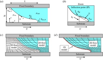
A hydrodynamic model is developed for the displacement of a receding fluid by an advancing fluid within a gap
 $H$
, where the top boundary is immobile and the bottom substrate moves horizontally at a speed
 $U$
(figure 1
a). The viscosities of the advancing and the receding fluids are denoted by
 ${\it\mu}_{adv}$
and
 ${\it\mu}_{rec}$
, respectively. Symbols
 $x$
and
 $y$
represent the Cartesian coordinates, and
 $s$
is the arclength along the fluid interface (located at
 $y=h$
) starting from the static (top) contact line. The horizontal length of the interface is denoted by
 $L$
.
Figure 1(b) shows the difference between the microscopic contact angle
 ${\it\theta}_{mic}$
and the dynamic (or macroscopic or apparent) contact angle
 ${\it\theta}_{M}$
. The angle
 ${\it\theta}_{mic}$
is the one at which the interface contacts the substrate, whereas
 ${\it\theta}_{M}$
, arising from the viscous bending of the interface, is measured at some distance away from the dynamic contact line. In this work, the maximum angle along the fluid interface is designated as
 ${\it\theta}_{M}$
and this position corresponds to the interface inflection point (IP). The height of the IP and the distance from the dynamic contact line to the IP are denoted by
 $h_{f}$
and
 $r_{f}$
, respectively. Note that
 ${\it\theta}_{mic,T}$
and
 ${\it\theta}_{mic,B}$
in figure 1(a) represent the microscopic contact angles at the top and the bottom substrates.
(a) Schematic of the problem geometry. (b) Enlarged view of the fluid interface and the inflection point (IP), which corresponds to the location of the maximum interface angle (
 ${\it\theta}_{M}$
). The height of the IP and the distance from the contact line to the IP are denoted by
 $h_{f}$
and
 $r_{f}$
, respectively. (c) Schematic of a full 2D approach. (d) Schematic of the 1D/2D hybrid approach.

To simplify the model, we neglect the influence of inertia so that Stokes equations apply to each phase:
 $$\begin{eqnarray}\boldsymbol{{\rm\nabla}}\boldsymbol{\cdot }\boldsymbol{v}=0,\quad \boldsymbol{{\rm\nabla}}p={\rm\nabla}^{2}\boldsymbol{v},\end{eqnarray}$$
where
 $\boldsymbol{v}$
and
 $p$
represent fluid velocity and pressure in a given phase. Note that lengths, velocities and stresses are non-dimensionalized with the characteristic scales
 $H$
,
 $U$
and
 ${\it\mu}U/H$
, respectively, with
 ${\it\mu}$
being the viscosity of a given phase.
The surfactants are assumed to be insoluble, and their transport along the fluid interface is governed by a steady-state convection–diffusion equation:
 $$\begin{eqnarray}\boldsymbol{{\rm\nabla}}_{s}\boldsymbol{\cdot }(\boldsymbol{v}_{s}{\it\Gamma})=\frac{1}{Pe}{\rm\nabla}_{s}^{2}\,{\it\Gamma},\end{eqnarray}$$
where
 $\boldsymbol{{\rm\nabla}}_{s}$
is the surface-gradient operator,
 $\boldsymbol{v}_{s}$
is the interface velocity, and
 ${\it\Gamma}$
is the dimensionless surfactant concentration scaled with the mean surfactant concentration
 ${\it\Gamma}_{m}$
at the interface. The surface Péclet number
 $Pe=UH/D_{s}$
contains the surface diffusion coefficient
 $D_{s}$
.
Following the convention of the dynamic-wetting literature, the capillary number
 $Ca$
(ratio of viscous forces to surface-tension forces) and the Marangoni number
 $M$
(ratio of surface-tension-gradient forces to viscous forces) are calculated based on the more viscous phase. These parameters appear in the following set of dimensionless boundary conditions along the fluid interface:
 $$\begin{eqnarray}\displaystyle & \displaystyle \boldsymbol{v}|_{rec}=\boldsymbol{v}|_{adv},\qquad & \displaystyle\end{eqnarray}$$
 $$\begin{eqnarray}\displaystyle & \displaystyle \boldsymbol{n}\boldsymbol{\cdot }\boldsymbol{v}=0,\qquad & \displaystyle\end{eqnarray}$$
 $$\begin{eqnarray}\displaystyle & \displaystyle M/{\it\delta}({\it\chi})\boldsymbol{{\rm\nabla}}_{s}{\it\sigma}\boldsymbol{\cdot }\boldsymbol{t}=\boldsymbol{n}\boldsymbol{\cdot }\unicode[STIX]{x1D64F}\boldsymbol{\cdot }\boldsymbol{t}|_{adv}-\boldsymbol{n}\boldsymbol{\cdot }\unicode[STIX]{x1D64F}\boldsymbol{\cdot }\boldsymbol{t}|_{rec},\qquad & \displaystyle\end{eqnarray}$$
 $$\begin{eqnarray}\displaystyle & \displaystyle {\it\kappa}(1/[Ca{\it\delta}({\it\chi})]+{\it\sigma}M/{\it\delta}({\it\chi}))=\left(\boldsymbol{n}\boldsymbol{\cdot }\unicode[STIX]{x1D64F}\boldsymbol{\cdot }\boldsymbol{n}|_{adv}-\boldsymbol{n}\boldsymbol{\cdot }\unicode[STIX]{x1D64F}\boldsymbol{\cdot }\boldsymbol{n}|_{rec}\right),\qquad & \displaystyle\end{eqnarray}$$
 $$\begin{eqnarray}\displaystyle & \displaystyle \left.\begin{array}{@{}c@{}}Ca={\it\mu}_{adv}U/{\it\sigma}_{m},\quad M=({\it\sigma}_{o}-{\it\sigma}_{m})/{\it\mu}_{adv}U\quad \text{and}\quad {\it\delta}({\it\chi})=1\quad \text{for}~{\it\chi}\leqslant 1;\\ Ca={\it\mu}_{rec}U/{\it\sigma}_{m},\quad M=({\it\sigma}_{o}-{\it\sigma}_{m})/{\it\mu}_{rec}U\quad \text{and}\quad {\it\delta}({\it\chi})=1/{\it\chi}\quad \text{for}~{\it\chi}>1\end{array}\right\}.\qquad & \displaystyle\end{eqnarray}$$
Here, (2.3)–(2.4) are the no-slip and no-penetration boundary conditions, and (2.5)–(2.6) represent interfacial stress balances along the tangential and normal directions. Subscripts ‘
 $adv$
’ and ‘
 $rec$
’ indicate properties in the advancing and receding phases, respectively. At the fluid interface, unit normal vector
 $\boldsymbol{n}$
points toward the receding phase and unit tangent vector
 $\boldsymbol{t}$
is in the same direction as arclength coordinate
 $s$
(figure 1
a). The term
 $\boldsymbol{{\rm\nabla}}_{s}{\it\sigma}$
in (2.5) denotes the surface-tension gradient along the interface,
 ${\it\kappa}$
in (2.6) represents the interface curvature, and
 $\unicode[STIX]{x1D64F}$
is the Newtonian stress tensor.
In these balances,
 $Ca{\it\delta}({\it\chi})={\it\mu}_{adv}U/{\it\sigma}_{m}$
,
 $M/{\it\delta}({\it\chi})=({\it\sigma}_{o}-{\it\sigma}_{m})/{\it\mu}_{adv}U$
, and
 ${\it\chi}={\it\mu}_{rec}/{\it\mu}_{adv}$
(see definitions for
 $Ca$
,
 $M$
and
 ${\it\delta}({\it\chi})$
in (2.7); the definitions are the same as those reported by Vandre et al.
Reference Vandre, Carvalho and Kumar2013). In the expressions for
 $Ca$
and
 $M$
,
 ${\it\sigma}_{o}$
is the surface tension of the surfactant-free solution and
 ${\it\sigma}_{m}$
is the mean surface tension corresponding to
 ${\it\Gamma}_{m}$
. In the absence of surfactant,
 ${\it\sigma}_{m}={\it\sigma}_{o}$
and the Marangoni stresses vanish (i.e.
 $M/{\it\delta}({\it\chi})=0$
). This limiting case was studied in our prior work (Vandre et al.
Reference Vandre, Carvalho and Kumar2012, Reference Vandre, Carvalho and Kumar2013, Reference Vandre, Carvalho and Kumar2014).
For simplicity, we assume that the surfactant is dilute enough to apply a linear equation of state (Jensen & Grotberg Reference Jensen and Grotberg1992; Rame Reference Rame2001; Kumar & Matar Reference Kumar and Matar2004; Craster & Matar Reference Craster and Matar2009):
 $$\begin{eqnarray}{\it\sigma}=1-{\it\Gamma}.\end{eqnarray}$$
Here, surface tension and surfactant concentration have been non-dimensionalized using the relations
 ${\it\sigma}^{\prime }={\it\sigma}_{m}+({\it\sigma}_{o}-{\it\sigma}_{m}){\it\sigma}$
and
 ${\it\Gamma}^{\prime }={\it\Gamma}_{m}{\it\Gamma}$
, where variables with a prime represent dimensional values (Craster & Matar Reference Craster and Matar2009). We also assume that surfactants do not deposit onto the solid surface from the fluid interface, so
 $\boldsymbol{n}\boldsymbol{\cdot }\boldsymbol{{\rm\nabla}}{\it\Gamma}=0$
is applied at the two ends of the fluid interface. These boundary conditions require that a constraint of constant surfactant mass be applied:
 $$\begin{eqnarray}\int _{S}{\it\Gamma}\,\text{d}s=S,\end{eqnarray}$$
where
 $S$
represents the total interface arclength.
A Navier-slip boundary condition is applied along the moving substrate to avoid the stress singularity caused by applying the no-slip boundary condition at the contact line (Huh & Scriven Reference Huh and Scriven1971; Dussan Reference Dussan1976; Chan et al. Reference Chan, Srivastava, Marchand, Andreotti, Biferale, Toschi and Snoeijer2013; Sibley, Nold & Kalliadasis Reference Sibley, Nold and Kalliadasis2015):
 $$\begin{eqnarray}\boldsymbol{t}_{s}\boldsymbol{\cdot }(\boldsymbol{v}-\boldsymbol{U})={\it\lambda}[\boldsymbol{n}_{s}\boldsymbol{\cdot }({\it\delta}({\it\chi})\boldsymbol{T})\boldsymbol{\cdot }\boldsymbol{t}_{s}],\end{eqnarray}$$
where
 ${\it\lambda}=l_{slip}/H$
is the dimensionless slip length, and
 $l_{slip}$
is the dimensional slip length. The function
 ${\it\delta}({\it\chi})$
is defined in (2.7), and
 $\boldsymbol{n}_{s}$
,
 $\boldsymbol{t}_{s},$
and
 $\boldsymbol{U}$
correspond to the substrate’s normal, tangent and velocity vectors, respectively. This slip boundary condition is applied along the entire bottom substrate and is able to recover the no-slip condition (
 $\boldsymbol{v}\rightarrow \boldsymbol{U}$
) for distances greater than
 $l_{slip}$
away from the dynamic wetting line. The no-slip boundary condition is applied to the top boundary and the no-penetration condition is applied to both the top and bottom boundaries.
In the hydrodynamic model, the microscopic contact angles
 ${\it\theta}_{mic}$
serve as boundary conditions at the two ends of the fluid interface (Blake Reference Blake2006). Generally,
 ${\it\theta}_{mic}$
may depend on the substrate speed
 $U$
and material properties such as
 ${\it\mu}$
and
 ${\it\sigma}$
(Kistler Reference Kistler and Berg1993). Here, we take the simplest view and assume that
 ${\it\theta}_{mic}$
is constant and equal to the static contact angle
 ${\it\theta}_{s}$
(Eggers Reference Eggers2005).
In order to isolate the influence of Marangoni stresses on wetting failure, we will assume that the microscopic contact angles are neutral at both contact lines (i.e.
 ${\it\theta}_{mic,T}={\it\theta}_{mic,B}=90^{\circ }$
) and remain unchanged by surfactants. In addition, the mean surface tensions
 ${\it\sigma}_{m}$
are kept the same for displacements in the absence and presence of Marangoni stresses. In § 6, these assumptions are relaxed to compare model predictions with experimental data.
The Stokes equations (2.1), surfactant-transport equation (2.2), and associated conditions (e.g. (2.3)–(2.10)) form the hydrodynamic model, which is evaluated with three approaches: (i) a 1D lubrication-type approach, (ii) a hybrid approach coupling a 1D description of the receding phase and a 2D description of the advancing phase, and (iii) an asymptotic theory of Cox (Reference Cox1986b ).
2.2. 1D model
The hydrodynamic model is simplified to a 1D equation system by using lubrication theory (Oron, Davis & Bankoff Reference Oron, Davis and Bankoff1997). To properly describe the curvature
 ${\it\kappa}$
of the interface during fluid displacement, a ‘quasi-parallel’ (QP) approximation is made in which the curvature gradients along the
 $x$
-coordinate are assumed to be equal to those along the arclength
 $s$
(
 $\text{d}{\it\kappa}/\text{d}x\approx \text{d}{\it\kappa}/\text{d}s$
) (Jacqmin Reference Jacqmin2004; Sbragaglia, Sugiyama & Biferale Reference Sbragaglia, Sugiyama and Biferale2008). Lubrication theory assumes that the flow is nearly parallel and that the interface slope is small. The QP approximation allows one to overcome the latter restriction by using the full curvature
 $\text{d}{\it\theta}/\text{d}s$
, where
 ${\it\theta}$
is the local interface angle (Jacqmin Reference Jacqmin2004; Snoeijer Reference Snoeijer2006; Vandre Reference Vandre2013; Vandre et al.
Reference Vandre, Carvalho and Kumar2013). This 1D approach is relatively simple to implement and thus it is of interest to see how its predictions compare to those from a more detailed approach such as the hybrid model (§ 2.3).
Using lubrication theory and the QP approximation, (2.1)–(2.7) can be simplified to
 $$\begin{eqnarray}\frac{\text{d}{\it\kappa}}{\text{d}s}=\frac{\text{d}^{2}{\it\theta}}{\text{d}s^{2}}=Ca{\it\delta}({\it\chi})\frac{\text{d}}{\text{d}x}\left(p_{adv}-p_{rec}\right)=F\left(h,Ca,{\it\lambda},{\it\chi},\frac{\text{d}{\it\Gamma}}{\text{d}x},M\right),\end{eqnarray}$$
where the curvature gradients along the arclength
 $\text{d}{\it\kappa}/\text{d}s$
balance the pressure gradients in the
 $x$
-direction from the two phases, as described by the function
 $F(h,Ca,{\it\lambda},{\it\chi},\text{d}{\it\Gamma}/\text{d}x,M)$
(see appendix A). Note that
 $p$
with subscripts is used to distinguish pressures in the advancing and receding phases. While the function
 $F$
accounts for flows due to surface-tension gradients, it does not account for the influence of surface-tension changes on the normal stress balance. Within the approximations used to derive (2.11), the latter effect is found to be an order-of-magnitude smaller relative to that of the mean surface tension and is thus neglected.
Similarly, the surfactant-transport equation (2.2) can be expressed as follows:
 $$\begin{eqnarray}\frac{\text{d}(u{\it\Gamma})}{\text{d}s}=\frac{1}{Pe}\frac{\text{d}^{2}{\it\Gamma}}{\text{d}s^{2}},\end{eqnarray}$$
where
 $u$
is the horizontal velocity component at the interface. This interfacial velocity depends on the same variables as the function
 $F$
(see appendix A). Note that the surfactant-transport equation (2.12) is coupled with (2.11) through the surface equation of state (2.8).
The following geometric relationships are used to obtain the interface height
 $h$
and
 $x$
-coordinate:
 $$\begin{eqnarray}\frac{\text{d}h}{\text{d}s}=-\text{sin}\,{\it\theta};\quad \frac{\text{d}x}{\text{d}s}=-\text{cos}\,{\it\theta}.\end{eqnarray}$$
To obtain the profiles of interface angle
 ${\it\theta}(s)$
, surfactant concentration
 ${\it\Gamma}(s)$
and interface height
 $h(s)$
, the governing equations (2.11)–(2.13) along with conditions (2.8) and (2.9) are solved with a second-order finite-difference method (Vandre et al.
Reference Vandre, Carvalho and Kumar2012).
2.3. Hybrid model
One way to evaluate the hydrodynamic model of § 2.1 is to use a full 2D description of both the advancing and receding phases. In our prior work (in which surfactants were absent), this was accomplished by discretizing both phases into finite elements (figure 1
c) (Vandre et al.
Reference Vandre, Carvalho and Kumar2012, Reference Vandre, Carvalho and Kumar2013, Reference Vandre, Carvalho and Kumar2014). Here, we use a less computationally intense approach that combines a 1D description of the receding phase while retaining a 2D description of the advancing phase (figure 1
d). This novel hybrid approach is motivated by the observations that (i) the receding fluid becomes long and slender as the interface deforms near the onset of wetting failure, and (ii) a 2D description of the advancing phase is needed to capture the correct streamline pattern in that phase (Vandre et al.
Reference Vandre, Carvalho and Kumar2012, Reference Vandre, Carvalho and Kumar2013). Such interface deformation is especially evident in air entrainment where
 ${\it\chi}\ll 1$
, which is the case of most interest in this paper. Note that the hybrid approach is distinct from the 1D approach of § 2.2, where 1D descriptions are used for both phases. In addition, the influence of surface-tension changes in both the normal and tangential stress balances is accounted for in the hybrid approach.
Lubrication theory and the QP approximation (§ 2.2) are applied to the receding phase to obtain equations involving the pressure and velocity in that phase:
 $$\begin{eqnarray}\displaystyle & \displaystyle Ah+\frac{1}{2}Bh^{2}+\frac{1}{6}\frac{\text{d}p}{\text{d}s}h^{3}=0, & \displaystyle\end{eqnarray}$$
 $$\begin{eqnarray}\displaystyle & \displaystyle \left.\frac{\partial u}{\partial y}\right|_{s}=B+\frac{\text{d}p}{\text{d}s}h,\quad \text{where}~A=\frac{{\it\chi}h+{\it\chi}{\it\lambda}u_{s}-\displaystyle \frac{1}{2}\displaystyle \frac{\text{d}p}{\text{d}s}h^{2}}{{\it\lambda}+h},~B=\frac{-{\it\chi}+A}{{\it\lambda}}, & \displaystyle\end{eqnarray}$$
 $u_{s}$
represents the horizontal interface velocity,
 $h$
is the interface height, and
 ${\it\lambda}=l_{slip}/H$
is the dimensionless slip length. The velocity gradient in (2.15) is evaluated at the interface.
In the advancing phase, a full 2D description ((2.1) and associated boundary conditions) is applied. In addition, the full convection–diffusion equation for surfactant transport ((2.2) and associated conditions) is used.
The 1D and 2D descriptions are coupled through the interfacial boundary conditions (2.3)–(2.6). Lubrication theory provides expressions for the normal and tangential stresses in the receding phase:
 $$\begin{eqnarray}\boldsymbol{n}\boldsymbol{\cdot }\unicode[STIX]{x1D64F}\boldsymbol{\cdot }\boldsymbol{t}|_{rec}\approx {\it\chi}\frac{\partial u}{\partial y};\quad \boldsymbol{n}\boldsymbol{\cdot }\unicode[STIX]{x1D64F}\boldsymbol{\cdot }\boldsymbol{n}|_{rec}\approx p.\end{eqnarray}$$
The equations governing the 1D and 2D descriptions are solved using the Galerkin finite-element method (FEM) with elliptic mesh generation (see appendix B). Mesh independence is determined by varying the number of elements until there is less than a 2 % variation in the values of
 $Ca^{crit}$
predicted from steady-state solution families. Since the interface tends to bend sharply near the contact line, elements are refined locally to resolve large gradients in the interface curvature. We found that to obtain mesh-independent solutions, element sizes near the contact line need to be less than
 $10^{-3}{\it\lambda}$
, where
 ${\it\lambda}$
is the dimensionless slip length in (2.10).
Advantages of the hybrid approach arise from its computational efficiency. Since the receding phase is described with a 1D model, the hybrid model reduces the number of variables by nearly 50 % in comparison to a full 2D flow model (Vandre et al. Reference Vandre, Carvalho and Kumar2012, Reference Vandre, Carvalho and Kumar2013) (figure 1 c,d). In addition, mesh quality for the advancing phase is improved because mesh lines do not need to be reconciled with those in the receding phase. These factors make the hybrid model a potentially powerful tool for studying fluid displacement in realistic coating systems that commonly include complicated geometries, complex liquid rheology and transport of surface-active agents.
2.4. Asymptotic theory
Cox developed an asymptotic theory relating the apparent contact angle
 ${\it\theta}_{ap}$
to the microscopic contact angle
 ${\it\theta}_{mic}$
and the capillary number
 $Ca$
during fluid displacement (Cox Reference Cox1986a
). Later, Cox extended the theory to account for insoluble surfactants and found the following relation (Cox Reference Cox1986b
):
 $$\begin{eqnarray}\left.\begin{array}{@{}c@{}}\displaystyle \frac{{\it\sigma}_{cox}}{q({\it\theta}_{ap};{\it\chi})}[g({\it\theta}_{ap};{\it\chi})-g({\it\theta}_{mic};{\it\chi})]=Ca\ln ({\it\lambda}_{cox}^{-1}),\\ \displaystyle g({\it\theta};{\it\chi})=\int _{0}^{{\it\theta}}\frac{q({\it\phi};{\it\chi})}{f({\it\phi};{\it\chi})}\,\text{d}{\it\phi},\\ \displaystyle q({\it\theta};{\it\chi})=\exp \left[\int _{0}^{{\it\theta}}\frac{h({\it\phi};{\it\chi})}{f({\it\phi};{\it\chi})}\,\text{d}{\it\phi}\right],\\ \displaystyle h({\it\phi};{\it\chi})=-2\left\{\frac{{\it\chi}[({\rm\pi}-{\it\phi})\cos {\it\phi}+\sin {\it\phi}]}{({\rm\pi}-{\it\phi})^{2}-\sin ^{2}{\it\phi}}+\frac{{\it\phi}\cos {\it\phi}-\sin {\it\phi}}{{\it\phi}^{2}-\sin ^{2}{\it\phi}}\right\},\\ \displaystyle f({\it\phi};{\it\chi})=2\sin {\it\phi}\left\{\frac{{\it\chi}({\rm\pi}-{\it\phi})}{({\rm\pi}-{\it\phi})^{2}-\sin ^{2}{\it\phi}}+\frac{{\it\phi}}{{\it\phi}^{2}-\sin ^{2}{\it\phi}}\right\},\end{array}\right\}\end{eqnarray}$$
where
 ${\it\sigma}_{cox}$
represents the dimensionless interfacial tension (scaled by a characteristic interfacial tension) far away from the contact line,
 ${\it\chi}={\it\mu}_{rec}/{\it\mu}_{adv}$
is the viscosity ratio, and
 ${\it\phi}$
is a dummy variable. The theory assumes that inertia and surfactant diffusion are negligible, and is limited to low-speed steady wetting with slowly varying interface angles (
 $Ca\ll 1$
and
 $Ca|\partial {\it\theta}/\partial x|\ll 1$
, respectively). In contrast to the 1D and hybrid approaches, the asymptotic theory does not use a 1D description of either phase.
There are several important differences between the parameters in the asymptotic theory and parameters introduced in § 2.1. The parameter
 ${\it\lambda}_{cox}=l_{mic}/l_{M}$
(assumed small) is the ratio between an arbitrary macroscopic length scale
 $l_{M}$
(
 $10~{\rm\mu}\text{m}{-}1$
mm) and a microscopic length scale
 $l_{mic}$
(
 ${\sim}1$
nm) (Hocking Reference Hocking1976; Blake Reference Blake2006; Sui, Ding & Spelt Reference Sui, Ding and Spelt2014). Although
 ${\it\lambda}_{cox}$
has a similar meaning to the dimensionless slip length
 ${\it\lambda}$
in the Navier-slip boundary condition (2.10), the values for these two parameters may not be the same in general (Kistler Reference Kistler and Berg1993; Sui & Spelt Reference Sui and Spelt2013). In addition,
 ${\it\theta}_{ap}$
need not equal
 ${\it\theta}_{M}$
. Because of the different non-dimensionalization of surface tension in the asymptotic theory,
 ${\it\sigma}_{cox}$
does not necessarily equal the mean surface tension
 ${\it\sigma}_{m}$
defined in (2.7). In spite of these differences, the asymptotic theory can be compared to the 1D and hybrid models by treating
 ${\it\lambda}_{cox}$
and
 ${\it\sigma}_{cox}$
as fitting parameters, and by assuming that
 ${\it\theta}_{ap}={\it\theta}_{M}$
.
The relation between
 ${\it\theta}_{ap}$
and
 $Ca$
is obtained numerically because the integral functions
 $g({\it\theta};{\it\chi})$
and
 $q({\it\theta};{\it\chi})$
in (2.17) lack analytical solutions. Values of
 ${\it\theta}$
in an array starting from
 ${\it\theta}_{mic}$
to 180° are substituted for
 ${\it\theta}_{ap}$
in the first equation of (2.17), and the corresponding
 $Ca$
values are then calculated. This method stops when
 ${\it\theta}\approx 180^{\circ }$
and the calculated capillary number is assumed to correspond to the critical capillary number
 $Ca^{crit}$
. We note that this is an assumption since the asymptotic theory is expected to break down as
 ${\it\theta}\rightarrow 180^{\circ }$
(Cox Reference Cox1986a
). Nevertheless, this assumption describes well the behaviour of
 $Ca^{crit}$
in the absence of surfactants (Vandre et al.
Reference Vandre, Carvalho and Kumar2013), so we are motivated to examine it here. The values of
 $Ca^{crit}$
obtained from the asymptotic theory can be compared to those obtained from the 1D model of § 2.2 and the hybrid model of § 2.3.
Before proceeding, we note a connection between the asymptotic theory and the 1D model of § 2.2. In the absence of surfactants, the 1D model has a form very similar to equations obtained from a long-wavelength theory valid for large slopes (Snoeijer Reference Snoeijer2006; Vandre Reference Vandre2013). The long-wavelength theory, which expands around Stokes flow in a wedge, is able to recover Cox’s asymptotic solution (Cox Reference Cox1986a ; Snoeijer Reference Snoeijer2006). In the presence of surfactants, we expect that the 1D model behaves similarly. A detailed analysis of this behaviour, an analysis for small Marangoni numbers, and extension of the asymptotic theory to better predict the wetting transition (Eggers Reference Eggers2005; Gao & Lu Reference Gao and Lu2013) are all beyond the scope of the present paper but would be interesting topics for future work.
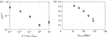
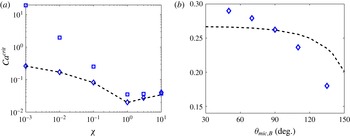
Comparison of critical capillary numbers in the absence of surfactant obtained from the full 2D flow model (circles) and the hybrid model (diamonds) while varying (a) fluid viscosity ratio and (b) substrate wettability. The relevant system parameters are (a)
 ${\it\lambda}=10^{-4}$
and
 ${\it\theta}_{mic,T}={\it\theta}_{mic,B}=90^{\circ }$
, (b)
 ${\it\chi}=10^{-3}$
,
 ${\it\lambda}=10^{-4}$
, and
 ${\it\theta}_{mic,T}=90^{\circ }$
.

3. Evaluation of the hybrid model in the absence of surfactants
In this section, we compare solutions from the hybrid model with those from a full 2D FEM calculation when surfactants are absent (Vandre et al.
Reference Vandre, Carvalho and Kumar2012, Reference Vandre, Carvalho and Kumar2013). These
 $Ca^{crit}$
values correspond to limit points in families of steady-state solutions, where a solution family takes the form of macroscopic contact angles
 ${\it\theta}_{M}$
as a function of the capillary number
 $Ca$
.
In figure 2(a),
 $Ca^{crit}$
values are plotted for various viscosity ratios
 ${\it\chi}$
. The hybrid model compares well with the full 2D flow model, especially when
 ${\it\chi}<1$
. Note that
 ${\it\chi}\ll 1$
corresponds to air/liquid displacement where the advancing phase is more viscous than the receding phase. Figure 2(b) shows that the agreement extends to various substrate wettabilities. The data remain restricted to partially wetting substrates where
 $50^{\circ }\leqslant {\it\theta}_{mic,B}\leqslant 130^{\circ }$
to avoid extensive distortion of the quadrilateral finite elements near the contact line. Note that
 ${\it\theta}_{mic,T}$
is fixed to 90° to isolate the influence of wettability of the bottom substrate.
The excellent agreement between the results from the hybrid and full 2D calculations in the case of air/liquid displacement (
 ${\it\chi}\ll 1$
) arises because viscous effects from the air are only important near the dynamic contact line, where the air flow is restricted to a slender wedge. Consequently, pressures in the air (receding phase) are well-described by lubrication theory and the QP approximation used in the hybrid model. Given the computational efficiency of the hybrid model and our interest in air entrainment (
 ${\it\chi}\ll 1$
), we use it rather than a full 2D FEM calculation to study the influence of insoluble surfactants.
4. Comparison between models
In this section, solutions from each approach described in § 2 are compared in the presence of surfactants. We make these comparisons for two reasons. First, we wish to test how well the predictions of
 $Ca^{crit}$
from the asymptotic theory of Cox (Reference Cox1986b
) compare to predictions from the other two approaches. In the absence of surfactants, similar comparisons were made in our prior work (Vandre et al.
Reference Vandre, Carvalho and Kumar2012, Reference Vandre, Carvalho and Kumar2013), but it has not yet been established how well the theory accounting for surfactants works. Second, we wish to test the limits of validity of the 1D approach. In the absence of surfactants, our prior work (Vandre et al.
Reference Vandre, Carvalho and Kumar2012, Reference Vandre, Carvalho and Kumar2013) shows that the 1D approach overpredicts
 $Ca^{crit}$
when the receding phase is much less viscous than the advancing phase (
 ${\it\chi}\ll 1$
) because it does not predict the correct streamline pattern in the advancing phase. However, when
 ${\it\chi}\geqslant 1$
, the 1D and 2D approaches give similar quantitative predictions. When Marangoni stresses due to surfactants are present, it is not yet clear how well the different predictions compare.
Unless stated otherwise, representative parameter values here and in § 5 are
 $10^{-3}\leqslant {\it\chi}\leqslant 10$
,
 ${\it\theta}_{mic,T}={\it\theta}_{mic,B}=90^{\circ }$
, and
 ${\it\lambda}=10^{-4}$
and
 $10^{-2}$
. An increase in
 ${\it\lambda}$
only increases the
 $Ca^{crit}$
values without changing the qualitative nature of the solutions presented in the remainder of the paper (results not shown). Note that the microscopic contact angle at the top substrate
 ${\it\theta}_{mic,T}$
is fixed to 90° in all cases, so we only present values of
 ${\it\theta}_{mic,B}$
in the remainder of the paper. The Marangoni number
 $M$
is taken as
 $0$
or
 $1$
to illustrate the cases where Marangoni stresses are absent and present, respectively. The Péclet number
 $Pe$
is taken as
 $10^{3}$
to represent the case of convection-dominated surfactant transport.
The macroscopic contact angles
 ${\it\theta}_{M}$
(maximum interface angle; § 2.1) are determined as a function of the capillary number
 $Ca$
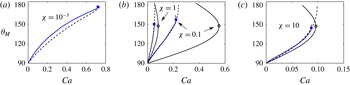
for various viscosity ratios and thus form steady-state solution families (figure 3). The solution families exhibit a limit point corresponding to the largest
 $Ca$
, which is denoted as the critical capillary number
 $Ca^{crit}$
. Beyond this
 $Ca^{crit}$
value (
 $Ca>Ca^{crit}$
), we are unable to find 2D steady-state solutions, suggesting that the system may develop transient or 3D flows leading to wetting failure (Vandre et al.
Reference Vandre, Carvalho and Kumar2013; Ledesma-Aguilar, Hernandez-Machado & Pagonabarraga Reference Ledesma-Aguilar, Hernandez-Machado and Pagonabarraga2013). For the 1D and hybrid models,
 $Ca^{crit}$
corresponds to a turning point in the solution paths that connects the stable (lower) and unstable (upper) branches of steady-state solutions.
Comparison of solution families in the presence of surfactant obtained from the asymptotic theory (dashed lines), 1D model (curves with open symbols), and hybrid model (curves with solid symbols) for various
 ${\it\chi}$
values: (a)
 ${\it\chi}=10^{-3}$
; (b)
 ${\it\chi}=1,0.1$
; (c)
 ${\it\chi}=10.$
Dashed lines denote the theoretical result in (2.17) with
 ${\it\lambda}_{cox}=0.07,{\it\theta}_{M}={\it\theta}_{ap}$
, and various
 ${\it\sigma}_{cox}$
values: (a)
 ${\it\sigma}_{cox}=1.70$
; (b)
 ${\it\sigma}_{cox}=0.78,1.15$
; (c)
 ${\it\sigma}_{cox}=0.92$
. Other parameter values are
 $M=1$
,
 $Pe=10^{3}$
,
 ${\it\lambda}=10^{-2}$
, and
 ${\it\theta}_{mic,B}=90^{\circ }$
.

For the asymptotic theory,
 $Ca^{crit}$
is assumed to coincide with the
 $Ca$
value at which the apparent angle
 ${\it\theta}_{ap}$
is 180°. Note that
 ${\it\theta}_{ap}$
in the asymptotic theory (2.17) is approximated as
 ${\it\theta}_{M}$
in figure 3. As discussed in § 2.4, the length scale ratio
 ${\it\lambda}_{cox}$
and the surface tension
 ${\it\sigma}_{cox}$
in (2.17) are treated as fitting parameters in order to compare solution families. Prior studies in the absence of surfactants suggest that the asymptotic theory has the best agreement with FEM calculations when
 ${\it\lambda}_{cox}\sim 10{\it\lambda}$
(Vandre et al.
Reference Vandre, Carvalho and Kumar2013). Therefore,
 ${\it\lambda}_{cox}$
is fixed to
 ${\sim}10{\it\lambda}$
and
 ${\it\sigma}_{cox}$
is tuned to match solution families from the asymptotic theory with those from the hybrid model.
Overall, figure 3 demonstrates that the asymptotic theory matches the lower (stable) branch of solution families predicted from the hybrid model over the entire
 ${\it\chi}$
range. In contrast, the 1D model only approximates well the hybrid model when
 ${\it\chi}\geqslant 1$
. For this reason, solution families from the 1D model are neglected in figure 3(a) where
 ${\it\chi}=10^{-3}$
. Similar behaviour is observed in the absence of surfactants (Vandre et al.
Reference Vandre, Carvalho and Kumar2012, Reference Vandre, Carvalho and Kumar2013).
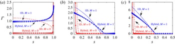
Figure 4 shows the surfactant concentration profiles obtained with the 1D model and the hybrid model for various viscosity ratios. (Because profiles from the asymptotic theory (Cox Reference Cox1986b
) cannot readily be extracted, they are not included in figure 4.) In the case where Marangoni stresses are absent (i.e.
 $M=0$
), the surfactants are passive and the fluid motion at the interface can be inferred from the concentration profiles. Note that the mean surface tensions
 ${\it\sigma}_{m}$
defined in the capillary and Marangoni numbers (2.7) are kept the same in both cases so that the only factor influencing concentration distributions is the surface-tension gradient.
Surfactant concentration profiles obtained with the 1D model and the hybrid model at (a)
 ${\it\chi}=10^{-3}$
; (b)
 ${\it\chi}=1$
; (c)
 ${\it\chi}=10.$
The concentration is plotted as a function of arclength coordinate
 $s$
for
 $M=1$
(blue dotted line),
 $M=0$
(red dash-dotted line) for the 1D model, and
 $M=1$
(blue diamonds),
 $M=0$
(red circles) for the hybrid model. In each plot
 $Ca=Ca^{crit}$
: (a)
 $Ca=0.72$
(hybrid) and
 $Ca=40.4$
(1D); (b)
 $Ca=0.05$
(hybrid) and
 $Ca=0.08$
(1D); (c)
 $Ca=0.088$
(hybrid) and
 $Ca=0.096$
(1D). Note that these plots only show part of the complete concentration profiles. The maximum concentrations in the case of
 $M=0$
are around (a) 300 (hybrid); (b) 35 (hybrid) and 25 (1D); (c) 75 (hybrid) and 70 (1D). Other parameter values are
 $Pe=10^{3}$
,
 ${\it\lambda}=10^{-2}$
, and
 ${\it\theta}_{mic,B}=90^{\circ }$
.

When
 $M=0$
and
 ${\it\chi}=10^{-3}$
(figure 4
a), the hybrid model predicts that surfactants are carried toward the dynamic contact line (
 $s=1$
), whereas the 1D model predicts that surfactants are carried toward the static contact line (
 $s=0$
). (Even in the absence of surfactants, the the 1D model predicts the incorrect streamline pattern for
 ${\it\chi}=10^{-3}$
(Vandre et al.
Reference Vandre, Carvalho and Kumar2012, Reference Vandre, Carvalho and Kumar2013).) As a consequence, when
 $M=1$
the Marangoni stresses predicted from the hybrid model are directed toward the static contact line and those from the 1D model toward the dynamic contact line. In contrast, in the cases where
 ${\it\chi}\geqslant 1$
(figure 4
b,c), surfactant concentration profiles from the 1D model compare well with those from the hybrid model, indicating that the same direction (toward the dynamic contact line) of Marangoni stresses is predicted from both approaches.
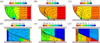
Figure 5 shows streamlines and pressure contours obtained from the 1D model and hybrid model when
 $M=1$
. For each viscosity ratio
 ${\it\chi}$
, streamlines from the hybrid model display a rolling-flow pattern in the advancing phase, which results from the viscous drag by the moving substrate. In the case of a low-viscosity receding phase (
 ${\it\chi}=10^{-3}$
), the rolling flow dominates the advancing phase and sets the direction of flow along the fluid interface (figure 5
a). A recirculation region is found near the top contact line, and this primarily results from the Marangoni stresses (see § 5.1 for an explanation). In contrast, in the cases where
 ${\it\chi}\geqslant 1$
, the receding phase dominates the fluid displacement and the interfacial flow. Therefore, the streamlines in the advancing phase split into two parts, with one following the rolling-flow pattern and the other forming a recirculation region near the interface (figure 5
b,c).
Streamlines and pressure contours obtained with the hybrid model (a–c) and the 1D model (d–f) in the presence of Marangoni stresses (
 $M=1$
): (a,d)
 ${\it\chi}=10^{-3}$
; (b,e)
 ${\it\chi}=1$
; (c,f)
 ${\it\chi}=10$
. Other parameter values are the same as those listed in figure 4 caption.

Similar to what is found in the absence of Marangoni stresses (Vandre et al.
Reference Vandre, Carvalho and Kumar2012, Reference Vandre, Carvalho and Kumar2013), the 1D model does not consider the flow created when the moving substrate drags the advancing phase. Therefore, streamlines from the 1D model are primarily determined by the receding phase and the Marangoni flow. When the receding-phase stresses are small (
 ${\it\chi}=10^{-3}$
), Marangoni stresses dominate and cause a recirculation zone in the advancing phase (figure 5
d). The receding-phase stresses cause another recirculation zone as the viscosity of that phase increases (figure 5
e, f).
Although the 1D model does not predict the streamline pattern well, the pressure contours still provide valuable insight into the fluid motion in the receding phase because the 1D description is also applied to the receding flow in the hybrid model. For each
 ${\it\chi}$
, adverse pressure gradients are developed in the receding phase to pump the receding fluid away from the contact line.
The influence of the viscosity ratio
 ${\it\chi}$
on the onset of wetting failure when
 $M=1$
is illustrated in figure 6(a), where
 $Ca^{crit}$
values obtained from the three approaches of § 2 are plotted. Similar to figure 3, the 1D model overestimates
 $Ca^{crit}$
when
 ${\it\chi}<1$
, whereas the asymptotic theory of Cox matches the hybrid model well. Figure 6(b) shows the effect of substrate wettability when
 ${\it\chi}=10^{-3}$
. Here the quantitative agreement between the asymptotic theory and hybrid model is not as good, although the trend predicted is similar. The resemblance between figures 2 and 6 suggests that wetting failure with (figure 6) and without (figure 2) Marangoni stresses is governed by similar physical mechanisms. In addition, comparison of
 $Ca^{crit}$
values from figures 2(b) and 6(b) indicate that Marangoni stresses decrease
 $Ca^{crit}$
over a broad range of microscopic contact angles. The physical mechanism responsible for this will be discussed in § 5.2.
Even though the 1D and hybrid models predict very different streamline patterns in the advancing phase, both models yield similar predictions for
 $Ca^{crit}$
when
 ${\it\chi}\geqslant 1$
. Since the receding phase becomes more dominant as
 ${\it\chi}$
increases, and both models use the same description of that phase, the prediction of
 $Ca^{crit}$
becomes less sensitive to the flow structure in the advancing phase as
 ${\it\chi}$
increases.
The results of this section demonstrate that the asymptotic theory (Cox Reference Cox1986b
) accounting for insoluble surfactants describes well the qualitative behaviour of
 $Ca^{crit}$
over a wide range of viscosity ratios. The results also show that the 1D model yields qualitatively incorrect predictions (i.e. opposite direction of Marangoni stresses) when the viscosity ratio is small (
 ${\it\chi}\ll 1$
). However, the 1D model may still be useful for studying liquid withdrawal or liquid–liquid displacement since its predictions are more accurate for
 ${\it\chi}\geqslant 1$
. Since we are primarily interested in the case of air entrainment (
 ${\it\chi}\ll 1$
), only the hybrid model is used for the results presented in § 5.
(a) Comparison of critical capillary number as a function of viscosity ratio obtained from the 1D model (squares), hybrid model (diamonds), and asymptotic theory (dashed line). (b) Critical capillary number as a function of substrate wettability when
 ${\it\chi}=10^{-3}$
. Other parameter values are
 $Pe=10^{3}$
,
 ${\it\lambda}=10^{-4}$
,
 ${\it\lambda}_{cox}=10{\it\lambda}=10^{-3}$
,
 $M=1$
, and
 ${\it\theta}_{mic,B}=90^{\circ }$
with
 ${\it\sigma}_{cox}=1.6,1.3,1,0.72,0.75,0.9$
for the asymptotic theory (from left to right) in (a), and
 ${\it\sigma}_{cox}=1.6$
in (b).

5. Influence of surfactants on wetting failure
In this section, the influence of Marangoni stresses on wetting failure during air/liquid displacement (
 ${\it\chi}=10^{-3}$
) is studied using the hybrid model. A physical explanation of the influence of Marangoni stresses on
 $Ca^{crit}$
is then proposed. At the end of this section, parametric studies with respect to the Marangoni number
 $M$
and Péclet number
 $Pe$
are presented.
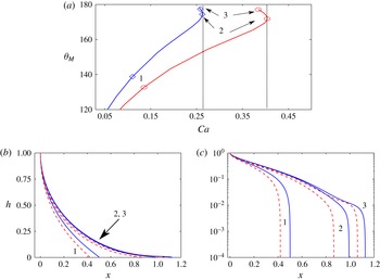
(a) Solution families obtained with the hybrid model near
 $Ca^{crit}$
for
 $M=1$
(blue curve with diamonds) and
 $M=0$
(red curve with circles). (b,c) Interface profiles corresponding to three different points along each solution family shown in (a). Blue solid and red dashed lines denote interfaces for
 $M=1$
and
 $M=0$
, respectively. Note that (c) is a semi-logarithmic plot. Other parameter values are
 ${\it\chi}=10^{-3}$
,
 $Pe=10^{3}$
,
 ${\it\lambda}=10^{-4}$
, and
 ${\it\theta}_{mic,B}=90^{\circ }$
.

5.1. Limit points
Figure 7 shows interface profiles for three wetting states along the steady-state solution paths when
 ${\it\chi}=10^{-3}$
. Figure 7(a) illustrates that the presence of Marangoni stresses (
 $M=1$
) decreases
 $Ca^{crit}$
, meaning that the Marangoni stresses promote the onset of wetting failure. Notably, Marangoni stresses also appear to increase the rate at which
 ${\it\theta}_{M}$
increases with
 $Ca$
. This is consistent with experimental observations of receding contact angles that decrease more quickly with contact-line speed when surfactant is present (Fell et al.
Reference Fell, Auernhammer, Bonaccurso, Liu, Sokuler and Butt2011, Reference Fell, Pawanrat, Bonaccurso, Butt and Auernhammer2012; Anyfantakis et al.
Reference Anyfantakis, Fell, Butt and Auernhammer2012). Figure 7(b,c) shows that interface deformation primarily occurs near the dynamic contact line as the interface elongates, which confirms the formation of a thin-film wedge in the receding phase (Kistler Reference Kistler and Berg1993; Marchand et al.
Reference Marchand, Chan, Snoeijer and Andreotti2012). Figure 7(b,c) also reveals that Marangoni stresses (
 $M=1$
) cause greater interface elongation, which implies that Marangoni stresses help the penetration of the receding air into the advancing liquid, thereby promoting wetting failure.
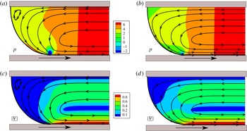
(a,b) Pressure contours and (c,d) velocity-magnitude contours obtained for
 $M=1$
(a,c) and
 $M=0$
(b,d). Other parameter values are
 $Ca=0.262$
for
 $M=1$
,
 $Ca=0.436$
for
 $M=0$
,
 ${\it\chi}=10^{-3}$
,
 $Pe=10^{3}$
,
 ${\it\lambda}=10^{-4}$
, and
 ${\it\theta}_{mic,B}=90^{\circ }$
.

Figure 8 compares pressure contours, streamlines, and velocity magnitudes for
 $M=0$
and
 $M=1$
near
 $Ca^{crit}$
. In both systems, the advancing phase is dragged by the moving substrate, which results in a rolling-flow pattern in that phase. However, the flow field for
 $M=1$
exhibits a recirculation region near the top contact line (figure 8
a). This is caused by Marangoni stresses, which act against the direction of the rolling flow and in turn drag the advancing fluid. The drag created by the Marangoni stresses can have a significant influence on the flow field near the top contact line because the fluid motion there is relatively slow (figure 8
c,d). In addition, the velocity magnitudes are also decreased by the Marangoni stresses in regions near the interface (figure 8
c); these stresses point toward the static contact line (figure 4
a). Overall, the plots in figure 8 demonstrate that Marangoni stresses have a significant influence on the flow field near the fluid interface.
5.2. Physical mechanisms
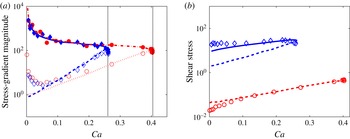
As suggested in § 4, the mechanism of wetting failure in the presence and absence of Marangoni stresses may be similar. In the absence of Marangoni stresses, wetting failure occurs when the capillary-stress gradients can no longer provide the pressure gradients required to pump the receding fluid away from the contact line (Vandre et al. Reference Vandre, Carvalho and Kumar2013). In this section, we study how this mechanism is modified when Marangoni stresses are present. As we will show, Marangoni stresses increase the receding-phase pressure gradients near the contact line by thinning the air film without significantly changing the capillary-pressure gradients there. As a result, wetting failure occurs at lower substrate speeds (capillary numbers).
(a) Magnitude of stress gradients at the IP for
 $M=1$
(blue diamonds) and
 $M=0$
(red circles). The capillary-stress gradients (filled symbols) match the receding-phase pressure gradients (open symbols) at
 $Ca^{crit}$
values denoted by vertical black dotted lines. Blue solid (
 $M=1$
) and red dash-dotted lines (
 $M=0$
) are from (5.2). Blue dashed (
 $M=1$
) and red dotted lines (
 $M=0$
) are from (5.1). (b) The magnitude of receding-phase shear stresses at the IP for
 $M=1$
(
 $(\boldsymbol{n}\boldsymbol{\cdot }\unicode[STIX]{x1D64F}\boldsymbol{\cdot }\boldsymbol{t})_{rec}$
) (blue diamonds) and
 $M=0$
(
 $(\boldsymbol{n}\boldsymbol{\cdot }\unicode[STIX]{x1D64F}\boldsymbol{\cdot }\boldsymbol{t})_{rec}$
) (red circles). Blue and red dashed lines are from (5.3) for
 $M=1$
and
 $M=0$
, respectively. Blue solid line is from (5.4) for
 $M=1$
. Other parameter values are
 ${\it\chi}=10^{-3}$
,
 $Pe=10^{3}$
,
 ${\it\lambda}=10^{-4}$
, and
 ${\it\theta}_{mic,B}=90^{\circ }$
.

According to lubrication theory, which is applied to the receding phase in the hybrid model, the receding-phase pressure gradients at the inflection point (IP) scale as
 $$\begin{eqnarray}\left|\frac{\text{d}p}{\text{d}x}\right|\sim \frac{{\it\chi}}{{h_{f}}^{2}},\end{eqnarray}$$
where
 ${\it\chi}$
is the viscosity ratio and
 $h_{f}$
represents the height of the IP (see figure 1
b). Because of the Navier-slip boundary condition (2.10) applied in the hybrid model, the interface curvature
 ${\it\kappa}$
near the dynamic contact line diverges as a function of
 $r$
(
 ${\it\kappa}\sim \ln (r)$
) (Snoeijer & Andreotti Reference Snoeijer and Andreotti2013; Vandre et al.
Reference Vandre, Carvalho and Kumar2013). Therefore, the capillary-stress gradients at the IP scale as
 $$\begin{eqnarray}\frac{1}{Ca}\left|\frac{\text{d}{\it\kappa}}{\text{d}x}\right|\sim \frac{1}{Ca}\left(\frac{1}{r_{f}}\right),\end{eqnarray}$$
where
 $r$
is the radial distance of the interfacial position from the contact line and
 $r_{f}$
represents the radial distance of the IP (see figure 1
b). Note that (5.2) is simplified from a more complicated expression for systems where
 $1/h_{f}\gg {\it\lambda}$
(Vandre et al.
Reference Vandre, Carvalho and Kumar2013).
Figure 9(a) shows the capillary-stress gradient and receding-phase pressure gradient as a function of
 $Ca$
. These gradients are equal at
 $Ca=Ca^{crit}$
for both
 $M=0$
and
 $M=1$
, confirming that the wetting-failure mechanism is similar in both cases. In addition, the scaling relationships (5.1) and (5.2) match the numerical results well. Notably, the pressure gradients when
 $M=1$
grow at a quicker rate than those when
 $M=0$
, and so match the capillary-stress gradients at a smaller
 $Ca^{crit}$
value. Interestingly, the values of the capillary-stress gradient do not change significantly. The presence of Marangoni stresses thus accelerates the onset of wetting failure by increasing the pressure gradients in the receding phase.
To investigate why Marangoni stresses increase the receding-phase pressure gradients, the receding-phase shear stresses at the IP are compared. As shown in figure 9(b), the receding-phase shear stresses when
 $M=1$
are stronger than those when
 $M=0$
; this is a consequence of the tangential stress balance (2.5). These stronger shear stresses mean that higher velocity gradients (
 $\text{d}u/\text{d}y$
) are needed near the interface. This is achieved by a thinning of the air film (air velocity changes over a smaller distance); the lower interfacial velocity (figure 8
c) also means that thinning is needed to increase the velocity gradient. Since the air film is thinned (
 $h_{f}$
decreases) in the presence of Marangoni stresses, the receding-phase pressure gradients are increased according to the scaling (5.1). Direct evidence of the air-film thinning will be presented below (figure 10
a).
In figure 9(b), scaling relationships for the receding-phase shear stresses are also included. According to lubrication theory, the shear stresses can be approximated as
 $$\begin{eqnarray}{\it\mu}_{rec}\left|\frac{\text{d}u}{\text{d}y}\right|\sim {\it\mu}_{rec}\frac{U}{h_{f}},\end{eqnarray}$$
where
 ${\it\mu}_{rec}$
is the receding-phase viscosity and
 $U$
is the substrate speed. As shown in figure 9(b), the above scaling matches the shear stresses in the case where
 $M=0$
(red dashed line) but a better scaling is needed for the case where
 $M=1$
,
 $$\begin{eqnarray}{\it\mu}_{rec}\left|\frac{\text{d}u}{\text{d}y}\right|\sim \frac{{\it\sigma}_{m}}{L},\end{eqnarray}$$
where
 ${\it\sigma}_{m}$
is the mean surface tension and
 $L$
represents the horizontal interface length (see figure 1). This expression reflects the fact that the surface tension determines the magnitude of the shear stresses which balance Marangoni stresses. As can be seen in figure 9(b), the scaling (5.4) agrees better with the numerical results (blue solid line).
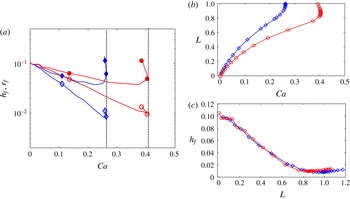
(a) Interfacial length scales
 $r_{f}$
(filled symbols) and
 $h_{f}$
(open symbols) as a function of
 $Ca$
for
 $M=1$
(blue diamonds) and
 $M=0$
(red circles). (b) Interfacial length
 $L$
plotted against
 $Ca$
for
 $M=1$
(blue diamonds) and
 $M=0$
(red circles). (c) Inflection-point height
 $h_{f}$
as a function of
 $L$
for
 $M=1$
(blue diamonds) and
 $M=0$
(red circles). Other parameter values are
 ${\it\chi}=10^{-3}$
,
 $Pe=10^{3}$
,
 ${\it\lambda}=10^{-4}$
, and
 ${\it\theta}_{mic,B}=90^{\circ }$
.

Figure 10(a) shows the change of the characteristic lengths (figure 1
b) at the IP with
 $Ca$
. For both
 $M=0$
and
 $M=1$
,
 $r_{f}$
and
 $h_{f}$
decrease with
 $Ca$
, which means that the IP approaches the dynamic contact line as
 $Ca$
increases and the air film is thinned and stretched. Both
 $r_{f}$
and
 $h_{f}$
when
 $M=1$
are smaller compared to the case when
 $M=0$
. This confirms that Marangoni stresses further thin the air film and explains the larger receding-phase pressure gradients when
 $M=1$
(figure 9
a).
Figure 10(b) demonstrates that the interfacial length
 $L$
when
 $M=1$
has a larger value compared to the case when
 $M=0$
, indicating that Marangoni stresses cause greater interface elongation and help the penetration of the receding phase (figure 7
b,c). Note that in both cases
 $L$
shows a sharp increase near
 $Ca^{crit}$
, consistent with experimental observations in the absence of surfactants (Burley & Kennedy Reference Burley and Kennedy1976).
To see how the air-film thickness changes with the interface elongation,
 $h_{f}$
is plotted as a function of
 $L$
for
 $M=0$
and
 $M=1$
(figure 10
c). As expected, the film is thinned as the interface elongates. However, the results for both cases collapse onto the same curve, which further supports the observation that the mechanism for wetting failure is very similar in the presence and absence of Marangoni stresses. This plot also highlights the key role played by the IP position. The presence of Marangoni stresses thins the air film and moves the IP closer to the dynamic contact line, bringing the system closer to wetting failure.
5.3. Influence of
 $M$
and
$Pe$


As defined by (2.7), the Marangoni number measures the strength of Marangoni stresses relative to viscous stresses, with larger values of
 $M$
corresponding to stronger Marangoni stresses. To satisfy the interfacial stress balance (2.5), the receding-phase shear stresses increase as
 $M$
increases. As discussed in § 5.2, this increase of shear stresses is produced by thinning of the air film, which in turn promotes the onset of wetting failure. As a result, the effect of Marangoni stresses on wetting failure is more pronounced as
 $M$
increases (figure 11
a). Note that surfactant concentration gradients are very large near the dynamic contact line when
 $M\rightarrow 0$
and
 $Pe=10^{3}$
, which causes the hybrid model to diverge. For this reason,
 $Ca^{crit}$
values in the
 $0<M<1$
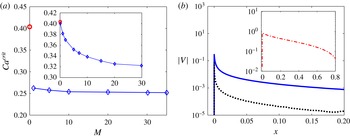
regime are only shown in the inset of figure 11(a), where
 $Pe=1$
.
(a) Critical capillary number as a function of the Marangoni number (
 $M$
) for
 $Pe=10^{3}$
. The data point for
 $M=0$
is denoted as a red circle. Inset: same plot but for
 $Pe=1$
. (b) Fluid-interface velocity magnitude at
 $Ca^{crit}$
as a function of the distance from the contact line for
 $M=1$
(blue solid line) and
 $M=50$
(black dotted line) when
 $Pe=10^{3}$
. Inset: velocity magnitude for
 $M=0$
. Other parameter values are
 ${\it\chi}=10^{-3}$
,
 ${\it\lambda}=10^{-4}$
, and
 ${\it\theta}_{mic,B}=90^{\circ }$
.

As
 $M$
increases, fluid displacement approaches an extreme case (
 $Ca^{crit}$
value shows a plateau in figure 11(a)), where the velocity magnitude
 $|V|$
of the fluid interface approaches zero, resulting in a no-slip condition (Tsai, Carvalho & Kumar Reference Tsai, Carvalho and Kumar2010). This is because strong Marangoni stresses counteract the rolling motion in the advancing phase. Consequently, the interfacial velocity is lowered with increasing
 $M$
as shown in figure 11(b). Note that the
 $x$
-coordinate in figure 11(b) is the distance from the contact line. The origin of the
 $x$
-coordinate represents the dynamic contact line, where the velocity is close to zero because of the Navier-slip boundary condition applied at the moving substrate (Vandre et al.
Reference Vandre, Carvalho and Kumar2012).
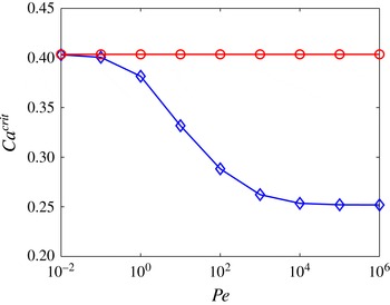
Figure 12 shows the impact of the Péclet number (
 $Pe$
) on wetting failure;
 $Pe$
provides a measure of the ratio between convective and diffusive transport of surfactants along the fluid interface. As diffusion becomes important (i.e.
 $D_{s}$
increases and
 $Pe$
decreases),
 $Ca^{crit}$
increases, which means that surfactants with larger
 $D_{s}$
can delay the onset of wetting failure. However, the systems with larger
 $D_{s}$
reduce to the case where Marangoni stresses are absent (i.e.
 $M=0$
). This is because diffusion tends to smooth surfactant concentration gradients along the interface, leading to smaller effects from Marangoni stresses. Therefore, the
 $Ca^{crit}$
value for
 $M=1$
is the same as that for
 $M=0$
when
 $Pe\leqslant 10^{-2}$
.
Critical capillary number as a function of the Péclet number (
 $Pe$
) for
 $M=1$
(blue diamonds) and
 $M=0$
(red circles). Other parameter values are
 ${\it\chi}=10^{-3}$
,
 ${\it\lambda}=10^{-4}$
, and
 ${\it\theta}_{mic,B}=90^{\circ }$
.

6. Comparison of model predictions with experimental data
As mentioned in § 1, surfactants can decrease the equilibrium surface tension and lower the static contact angle
 ${\it\theta}_{s}$
, and surface-tension gradients can induce Marangoni stresses. In this section, our model predictions are compared with experimental data from Burley & Kennedy (Reference Burley and Kennedy1976), whose experimental setup is similar to our model geometry.
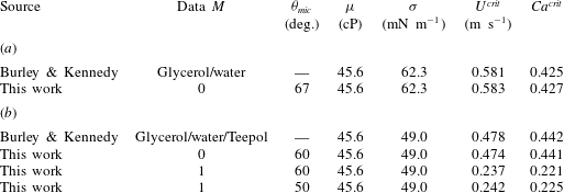
Burley and Kennedy recorded the critical speed
 $U^{crit}$
at which wetting failure (i.e. air entrainment) occurs when a polyethylene terephthalate (PET) tape plunges into a tank of liquid (glycerol/water) (Burley & Kennedy Reference Burley and Kennedy1976). They found that the presence of Teepol detergent, which contains mixture of soluble surfactants, lowers the critical speed by up to 17.5 % (see
 $U^{crit}$
in table 1). To characterize the influence of surfactants on wetting failure,
 $Ca^{crit}$
values are calculated based on the definition in (2.7) by substituting in the liquid viscosity
 ${\it\mu}$
and surface tension
 ${\it\sigma}$
reported in the experimental study (see
 $Ca^{crit}$
in table 1).
Based on the experimental data,
 $M=0$
(glycerol/water),
 $M=1$
(glycerol/water/Teepol), and
 ${\it\chi}=4\times 10^{-4}$
. In our previous study without surfactants (Vandre et al.
Reference Vandre, Carvalho and Kumar2012), our full 2D FEM calculation accurately described experimental data in a similar geometry for
 ${\it\lambda}\leqslant 10^{-5}$
. Therefore,
 ${\it\lambda}=10^{-5}$
is chosen here. Since the static contact angles (
 ${\it\theta}_{mic}$
) are not given by Burley & Kennedy (Reference Burley and Kennedy1976), we choose 67° for the glycerol/water system (Vandre et al.
Reference Vandre, Carvalho and Kumar2014) and 50° for the glycerol/water/Teepol system. Note that the lowest limit of the hybrid model, 50°, is picked due to the lack of contact-angle data in the literature for the glycerol/water/Teepol mixture on PET. In addition, because the type of Teepol is not specified in Burley and Kennedy’s work, the diffusion coefficient
 $D_{s}$
is chosen from values of common lab surfactants (Shen et al.
Reference Shen, Gleason, McKinley and Stone2002) (
 $D_{s}\sim 10^{-10}~\text{m}^{2}~\text{s}^{-1}$
) and, therefore,
 $Pe=10^{6}$
for the model.
Comparison between model predictions and published experimental data from Burley & Kennedy (Reference Burley and Kennedy1976) in (a) surfactant-free and (b) surfactant-loaded systems. Other parameter values for the hybrid model are
 ${\it\chi}=4\times 10^{-4}$
and
 ${\it\lambda}=10^{-5}$
.

A comparison between model predictions and experimental values of
 $U^{crit}$
shows good agreement in the absence of surfactants (table 1
 $\!a$
). Surprisingly,
 $U^{crit}$
calculated from the case
 $M=0$
and
 ${\it\theta}_{mic}=60^{\circ }$
matches the experimental value of
 $U^{crit}$
in the presence of surfactants (table 1
 $\!b$
). However, when Marangoni stresses are present in the model (
 $M=1$
,
 ${\it\theta}_{mic}=60^{\circ }$
), the predicted critical speed
 $U^{crit}$
is much smaller (
 ${\sim}$
50 %) than the experimental value. As
 ${\it\theta}_{mic}$
is lowered (
 $M=1$
,
 ${\it\theta}_{mic}=50^{\circ }$
), both
 $U^{crit}$
and
 $Ca^{crit}$
are increased, although these values are still much smaller than the experimental values.
Although uncertainty in the experimental values of the contact angle prevents us from drawing more definitive conclusions, the comparison shown in table 1 suggests that changes in
 $U^{crit}$
observed by Burley & Kennedy (Reference Burley and Kennedy1976) upon the addition of surfactants are probably produced by a lowering of the mean surface tension and equilibrium contact angle, rather than by Marangoni stresses. Marangoni stresses may still be present in the experiment, but their effects may be much weaker than predicted by our model due to surfactant solubility, which would tend to lower surface-tension gradients via transport between the fluid interface and bulk. Weaker Marangoni stresses (smaller Marangoni numbers) would raise the value of
 $Ca^{crit}$
predicted by the model and probably bring it closer to the experimental value.
7. Conclusion
A hydrodynamic model is developed in this work to investigate the influence of insoluble surfactants on dynamic wetting failure. It is found that Marangoni stresses increase the rate at which the dynamic contact angle in our geometry increases with contact-line speed, consistent with experimental observations of the behaviour of receding contact angles in surfactant solutions (Fell et al.
Reference Fell, Auernhammer, Bonaccurso, Liu, Sokuler and Butt2011, Reference Fell, Pawanrat, Bonaccurso, Butt and Auernhammer2012; Anyfantakis et al.
Reference Anyfantakis, Fell, Butt and Auernhammer2012). The hydrodynamic model shows that 2D steady wetting fails at a critical substrate speed corresponding to a critical capillary number
 $Ca^{crit}$
. When the receding phase has a viscosity much less than the advancing phase, the 1D approach overestimates
 $Ca^{crit}$
and incorrectly predicts the direction of surfactant concentration gradients. However, since the 1D approach becomes more accurate as the viscosity of the receding phase increases, it may still be useful for studying liquid withdrawal or liquid–liquid displacement. The asymptotic theory of Cox (Reference Cox1986b
) is found to match well predictions from the 1D/2D hybrid approach over a wide range of viscosity ratios.
Analysis of our results reveals that the physical mechanism for wetting failure is similar in the absence and presence of Marangoni stresses. Wetting failure occurs when the fluid interface cannot provide the pressure gradients needed to pump air away from the contact line. The presence of Marangoni stresses promotes the onset of wetting failure by thinning the air film, which increases receding-phase pressure gradients near the contact line but does not significantly change the capillary-pressure gradients there.
The results of the present work have allowed us to establish how insoluble surfactants influence wetting failure through Marangoni stresses, and to gain insight into the decades-old experimental observations of Burley & Kennedy (Reference Burley and Kennedy1976). Our findings provide a strong motivation for accounting for surfactant solubility in future work, and for comparing model predictions to the other experimental observations in more complex geometries described in § 1. The hybrid model introduced here provides an especially efficient way to explore this issue, since in processes such as slot coating and curtain coating the dominant effects of the receding phase will be produced by the thin air film near the contact line.
Acknowledgements
We are grateful to the Donors of the American Chemical Society Petroleum Research Fund for initial support of this work, and to the National Science Foundation (CBET-1434016) for subsequent support.
Appendix A. Functions in the 1D model
The formulation of the 1D model in § 2.2 follows previous derivations (Jacqmin Reference Jacqmin2004; Sbragaglia et al.
Reference Sbragaglia, Sugiyama and Biferale2008; Vandre et al.
Reference Vandre, Carvalho and Kumar2012). However, we also consider the surface-tension-gradient term in tangential-stress balance equation (2.5). The function
 $F(h,Ca,{\it\lambda},{\it\chi},\text{d}{\it\Gamma}/\text{d}x,M)$
in (2.11) becomes
 $$\begin{eqnarray}\displaystyle & & \displaystyle F(h,Ca,{\it\lambda},{\it\chi},\text{d}{\it\Gamma}/\text{d}x,M)=-\!\{\!3Ca[-M\,\text{d}{\it\Gamma}/\text{d}x(h^{4}(-1+{\it\chi})-2{\it\lambda}(1+4{\it\lambda}){\it\chi}\nonumber\\ \displaystyle & & \displaystyle \qquad +\,h(-1+2{\it\lambda}+16{\it\lambda}^{2}){\it\chi}+h^{2}(1+2{\it\lambda})(-4{\it\lambda}(-1+{\it\chi})+3{\it\chi})\nonumber\\ \displaystyle & & \displaystyle \qquad +\,h^{3}(1-3{\it\chi}-2{\it\lambda}(1+{\it\chi})))+2(-h^{2}(-1+{\it\chi})(3{\it\chi}+4{\it\lambda}{\it\chi})\nonumber\\ \displaystyle & & \displaystyle \qquad +\,h{\it\chi}((-2+3{\it\chi})+2{\it\lambda}(-3+4{\it\chi}))+h^{3}(-1+{\it\chi}){\it\chi}-{\it\chi}({\it\chi}+4{\it\lambda}{\it\chi}))]\!\}\nonumber\\ \displaystyle & & \displaystyle \qquad /\!\{\!2h(h-1)[h^{3}(-1+{\it\chi})+3{\it\lambda}(1+4{\it\lambda}){\it\chi}+h(-2{\it\lambda}(-2+{\it\chi})\nonumber\\ \displaystyle & & \displaystyle \qquad -\,12{\it\lambda}^{2}(-1+{\it\chi})+{\it\chi})-h^{2}(-1+{\it\lambda}+2{\it\chi}+{\it\lambda}{\it\chi})]\!\}.\end{eqnarray}$$
The function
 $u$
in (2.12) becomes
 $$\begin{eqnarray}\displaystyle & & \displaystyle u=\{[(-1+h)h{\it\chi}(M\,\text{d}{\it\Gamma}/\text{d}x(-h+h^{2}-4{\it\lambda}(1+4{\it\lambda}))-2((-1+h-4{\it\lambda}){\it\chi}))]\nonumber\\ \displaystyle & & \displaystyle \qquad /\![4(h^{3}(-1+{\it\chi})+3{\it\lambda}(1+4{\it\lambda}){\it\chi}+h(-2{\it\lambda}(-2+{\it\chi})-12{\it\lambda}^{2}(-1+{\it\chi})+{\it\chi})\nonumber\\ \displaystyle & & \displaystyle \qquad -\,h^{2}(-1+{\it\lambda}+2{\it\chi}+{\it\lambda}{\it\chi}))]\!\}/{\it\chi}.\end{eqnarray}$$
Appendix B. Finite-element method for the hybrid model
We describe here some of the details associated with the Galerkin finite-element method (FEM) used to solve the governing equations of the hybrid model (§ 2.3).
Since FEM uses the weak form of the 2D governing equations (Christodoulou, Kistler & Schunk Reference Christodoulou, Kistler, Schunk, Kistler and Schweizer1997), the normal and tangential stresses in (2.16) cannot be directly applied to the fluid interface, but must be converted into an effective traction vector:
 $$\begin{eqnarray}\boldsymbol{n}\boldsymbol{\cdot }\unicode[STIX]{x1D64F}|_{rec}=\left\{{\it\chi}n_{y}\frac{\partial u}{\partial y}-n_{x}p,-{\it\chi}n_{x}\frac{\partial u}{\partial y}-n_{y}p\right\},\end{eqnarray}$$
where subscripts indicate the
 $x$
and
 $y$
components of the normal vector
 $\boldsymbol{n}$
at the fluid interface. Note that (2.16) is recovered from the normal and tangential projections of (B 1). The velocity gradient can be expressed in terms of the pressure and interface height through (2.15).
The following weak-form residual is applied to the advancing phase and the fluid interface:
 $$\begin{eqnarray}R_{hybrid}^{i}=-\int _{S}{\it\phi}_{i}\left(\frac{1}{Ca}\frac{\text{d}\boldsymbol{t}}{\text{d}s}+\boldsymbol{n}\boldsymbol{\cdot }\unicode[STIX]{x1D64F}|_{rec}+\frac{\text{d}{\it\sigma}}{\text{d}s}\boldsymbol{t}\right)\,\text{d}S+\int _{{\it\Omega}}{\it\phi}_{i}\left(-{\rm\nabla}^{2}\boldsymbol{v}+\boldsymbol{{\rm\nabla}}p\right)\,\text{d}{\it\Omega},\end{eqnarray}$$
where
 ${\it\phi}_{i}$
is the basis function,
 $s$
is the interface arclength,
 ${\it\Omega}$
is the area of the advancing phase, and
 $S$
is the interface length. Along the interface,
 $\text{d}\boldsymbol{t}/\text{d}s$
represents interface curvature and
 $(\text{d}{\it\sigma}/\text{d}s)\boldsymbol{t}$
is the surface-tension-gradient term. The unit normal vector
 $\boldsymbol{n}$
points toward the receding phase and the unit tangent vector
 $\boldsymbol{t}$
is in the same direction as the arclength
 $s$
. The traction vectors of the receding phase,
 $\boldsymbol{n}\boldsymbol{\cdot }\unicode[STIX]{x1D64F}|_{rec}$
, act as ‘loading’ terms that influence the flow of the advancing phase.
The receding phase also has a weak-form residual associated with it:
 $$\begin{eqnarray}R_{rec}^{i}=\int _{S}{\it\phi}_{i}\left(Ah+\frac{1}{2}Bh^{2}+\frac{1}{6}\frac{\text{d}p}{\text{d}s}h^{3}\right)\text{d}S.\end{eqnarray}$$
This residual is applied along the fluid interface. Note that the QP approximation (
 $\text{d}x\approx \text{d}s$
) is applied in (2.14)–(2.15) to express pressure gradients with respect to the arclength
 $s$
, which allows direct integration of weak-form residuals in FEM (Vandre Reference Vandre2013).
Along the fluid interface, surfactant transport is incorporated through the following weak-form residual:
 $$\begin{eqnarray}R_{surfactant}^{i}=\int _{S}{\it\phi}_{i}\left(\boldsymbol{{\rm\nabla}}_{s}\boldsymbol{\cdot }(\boldsymbol{v}_{s}{\it\Gamma})-\frac{1}{Pe}{\rm\nabla}_{s}^{2}{\it\Gamma}\right)\text{d}S.\end{eqnarray}$$
Because we assume that surfactants do not deposit onto solid boundaries, surfactant concentrations should satisfy the global constraint (2.9) to have a non-trivial solution.
In the advancing phase, biquadratic basis functions are used for velocity and linear discontinuous basis functions are used for pressure. Position variables (e.g.
 $h$
) are described with biquadratic basis functions. Only the receding-phase pressure at the interface is needed (see (B 3)), so it and the surfactant concentration are also described with biquadratic basis functions. The nodes along the fluid interface can thus be thought of as forming ‘1D elements’ for these variables.
Solution of the residual equations proceeds in a manner analogous to a full 2D FEM calculation (Vandre et al. Reference Vandre, Carvalho and Kumar2012, Reference Vandre, Carvalho and Kumar2013). The physical system is mapped to a computational domain using elliptic mesh generation (which introduces additional residual equations) (Christodoulou et al. Reference Christodoulou, Kistler, Schunk, Kistler and Schweizer1997). The field variables are represented by basis functions, and the resulting set of algebraic equations for the basis-function coefficients are then solved by the Newton–Raphson method using a frontal solver (Hood Reference Hood1976). Note that the global constraint (2.9) is incorporated into the frontal solver through the Woodbury formula (Press et al. Reference Press, Teukolsky, Vetterling and Flannery2007).