1 Introduction
Fluid-driven fractures are frequently investigated in the context of hydraulic fracturing operations mainly performed in the oil and gas industry. The technology, which has been around since the 1950s, has taken a major leap forward in the last decades as a result of increased product prices and improved technology for drilling, fracturing fluids, propping agents and pumping systems, and is currently heavily used in many parts of the world (Holditch Reference Holditch2007).
Hydraulic fracturing is the use of viscous fluids along with chemical additives to stimulate the deformation of an impermeable rock or tight sand structure. The method employs viscous fluids, consisting primarily of water, either fresh or recycled, along with chemicals used to modify the water characteristics (for example, to reduce friction or corrosion) and sand or other agents, referred to as ‘proppants’, which hold open the fractures created in the formation. Typically, many million litres of normal surface or ground water plus sand and chemical additives are injected and pressurized into an individual well to accomplish fracturing and release of hydrocarbons from shales. No two shales are alike, yet it is estimated that up to 50 % of the injected volume flows back to the surface on release of pressure and only a relatively small percentage of the returning volume is successfully recycled (King et al. Reference King2010).
Hydraulic fracturing and the production of hydrocarbons from fractured wells yield fluid wastewater that must be managed carefully to avoid significant harm to human health and the environment. These wastewater by-products are known as ‘flowback’ or ‘produced water’. Flowback periods immediately following fracture stimulation can be used quantitatively to characterize hydraulic fractures and in some cases the reservoir (Clarkson & Williams-Kovacs Reference Clarkson and Williams-Kovacs2013). Furthermore, flowback data provide an additional early opportunity to derive key properties affecting well performance and conductivity.
The problem of fracture propagation in an elastic medium has been studied extensively. In one approach the system is modelled using a combination of lubrication theory for the flow and the equations of linear elasticity. For example, Hubbert & Willis (Reference Hubbert and Willis1972) have investigated the elastic stress field and its effect on fracture orientation, while Spence & Sharp (Reference Spence and Sharp1985), Lister (Reference Lister1990) and Savitski & Detournay (Reference Savitski and Detournay2002) have offered two-dimensional models for the propagation of both buoyancy- and pressure-driven fractures in an elastic half-space. Lai et al. (Reference Lai, Zheng, Dressaire, Wexler and Stone2015, Reference Lai, Zheng, Dressaire and Stone2016b
) have presented experimental work for the case of an elastic penny-shaped pressure-driven hydraulic fracture propagation. Interest in such problems has been primarily driven by questions relating to creation and propagation of such fluid-driven fractures. However, recent environmental concerns have inspired the investigation of backflow mechanisms in single fractures. For example, Lai et al. (Reference Lai, Zheng, Dressaire, Ramon, Huppert and Stone2016a
) presented experimental results of an elastic model that show that when a liquid-filled crack closes up, only the thickness of the crack decreases while the radius of the crack remains nearly unchanged during the backflow process. Their late-time results are in good agreement with scaling arguments predicting that the liquid volume in the fracture decays with time according to
 $t^{-1/3}$
.
In this paper, we explore the behaviour of fluid-filled networks consisting of repeatedly bifurcating channels with elastic boundaries, as they relax from a pre-strained state, which generates a backflow of the fluid within each channel. The main assumptions guiding our work are: (i) the process of hydraulic fracturing propagates a network of fractures; (ii) the network relaxes under a linear elastic response to the strained state, and is resisted by the pressure developed in the viscous fluid, while retaining a constant fracture radius or length in the respective radial or Cartesian coordinates. Previous studies of similar problems have shown that the fluid mass in the medium should exhibit a power-law behaviour at late times. For example, Spence & Sharp (Reference Spence and Sharp1985), Lai et al. (Reference Lai, Zheng, Dressaire and Stone2016b ) addressed the dynamics of a single crack driven by elasticity. This work aims at demonstrating similar behaviour for network structures. A recent work by Chau, Bažant & Su (Reference Chau, Bažant and Su2016) investigating the growth of branched three-dimensional hydraulic crack systems concluded that the resulting network is expected to consist of roughly orthogonal vertical cracks and that V-shaped branching is not a realistic hypothesis for static crack growth. The work presented here makes use of a simple bifurcating model to envision the complex nature of such a network but neglects angle and end effects, so can be considered to be consistent with a variety of existing ideas on the geometric nature of the network. To the knowledge of the authors, the backflow dynamics for a fracture network has not been studied analytically before, which is the focus of the current work.
Herein, we study three model fracture systems. In § 2 we formulate and solve the case of a single fracture represented by two parallel rigid plates. In § 3 we present a formulation and solutions for the case of a network with a single bifurcation, and finally in § 4 we generalize the problem to the case of
 $n$
fracture generations in a bifurcated network. Numerical solutions are presented and compared with late-time asymptotic analysis. In § 5, we conclude the paper by discussing the implications for industrial and geological processes.
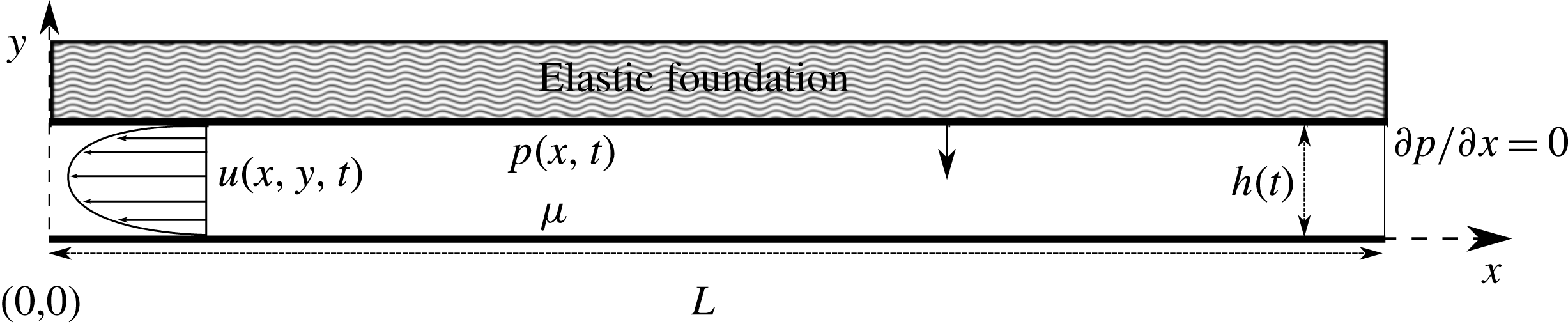
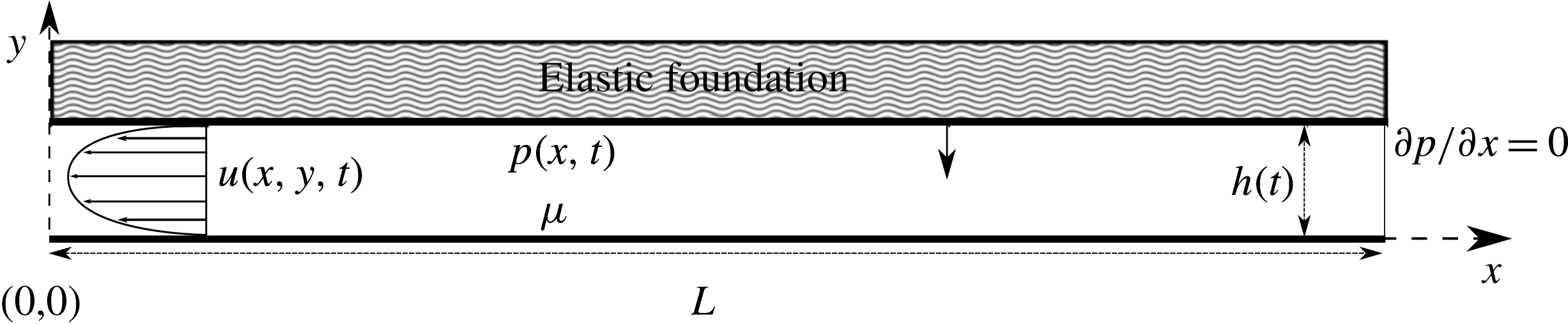
A schematic representation of a two-dimensional fracture of constant length
 $L$
and initial thickness
 $h^{\ast }=h(t=0)$
. At time
 $t>0$
the upper plate is forced down by the elastic response to a pre-strained condition against the viscous fluid. Since there is no flux at
 $x=L$
, a pressure gradient forms in the
 $x$
direction and results in a parabolic velocity profile towards the outlet at
 $x=0$
.
2 Single-fracture backflow dynamics
We begin our formulation of the backflow problem with a simple representation of a fracture filled with a viscous, incompressible fluid, confined in a bounded elastic medium. The fracture is envisioned as two rigid parallel plates of finite length
 $L$
with initial aperture
 $h^{\ast }$
, as shown in figure 1. The rigidity of the plates and the flat geometry imply that
 $h$
is constant in
 $x$
and dependent on time alone. The formulation is developed in the limit that the rigidity of the walls is sufficient to ensure that apertures are uniform throughout the fracture. This limit can be estimated using scaling of the basic plate theory equation (Landau & Lifshitz Reference Landau and Lifshitz1986, p. 42), which demands the scale of deflection to be much smaller than the aperture scale
 $h^{\ast }$
, or
 $$\begin{eqnarray}\displaystyle D\gg \frac{pL^{4}}{h^{\ast }}, & & \displaystyle\end{eqnarray}$$
where
 $D$
is the flexural rigidity or bending modulus of the solid and
 $p$
is the pressure in the fracture. Although this limit does not necessarily apply for all times, it is taken herein as a simplification to allow for other complexities that arise from applying this formulation to a network of fractures as will be shown in the following sections. The fracture is then squeezed shut by the elastic response to a pre-strained condition of the upper plate, which drives the flow. At time
 $t=0$
the upper plate is released and the fluid is squeezed out of the outlet at
 $x=0$
(figure 1).
2.1 Governing equations
Under the assumption that the fracture aperture is much smaller than its length (i.e.
 $h^{\ast }\ll L$
), we invoke the lubrication approximation for the quasi-steady fluid flow between the plates. We denote
 $p(x,t)$
as the fluid pressure inside the fracture and
 $u(x,y,t)$
as the velocity field in the negative
 $x$
-direction (i.e. towards the outlet), for convenience. The boundary conditions imposed are no-slip at both the top and bottom plates, yielding a parabolic velocity profile, which is then averaged vertically and leads to the averaged horizontal velocity (Batchelor Reference Batchelor2000, p. 220)
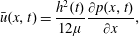 $$\begin{eqnarray}\displaystyle \bar{u}(x,t)=\frac{h^{2}(t)}{12\unicode[STIX]{x1D707}}\frac{\unicode[STIX]{x2202}p(x,t)}{\unicode[STIX]{x2202}x}, & & \displaystyle\end{eqnarray}$$
where
 $\unicode[STIX]{x1D707}$
is the dynamic viscosity. The corresponding one-dimensional continuity equation is
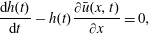 $$\begin{eqnarray}\displaystyle \frac{\text{d}h(t)}{\text{d}t}-h(t)\frac{\unicode[STIX]{x2202}\bar{u}(x,t)}{\unicode[STIX]{x2202}x}=0, & & \displaystyle\end{eqnarray}$$
where we assume the top and bottom plates are parallel and impermeable and the minus sign arises from the choice of the sign of
 $\bar{u}$
. Substituting (2.2) into (2.3), we obtain a nonlinear equation for the aperture
 $h(t)$
of a single fracture in the form of a Reynolds equation,
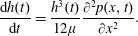 $$\begin{eqnarray}\displaystyle \frac{\text{d}h(t)}{\text{d}t}=\frac{h^{3}(t)}{12\unicode[STIX]{x1D707}}\frac{\unicode[STIX]{x2202}^{2}p(x,t)}{\unicode[STIX]{x2202}x^{2}}. & & \displaystyle\end{eqnarray}$$
A dynamic boundary condition is needed to account for the squeezing force driving the flow. We then introduce a simple model for a loaded plate bounding an elastic foundation. Since the plates are considered rigid and since deformation is independent of
 $x$
, we use the Winkler model (Kerr Reference Kerr1964) where the elastic response is represented as an array of springs obeying Hooke’s law, with
 $\hat{E}$
denoting the effective spring constant of the Winkler support (which for a thin elastic layer would be its Young’s modulus,
 $E$
, divided by its thickness
 $l_{0}$
). At time
 $t=0$
the spring begins to relax back to its original length and is resisted by the pressure developed in the fluid. The resulting force balance may be written as
 $$\begin{eqnarray}\displaystyle \int _{0}^{L}p(x,t)\,\text{d}x=\hat{E}Lh(t). & & \displaystyle\end{eqnarray}$$
An initial condition for
 $h(t)$
and two boundary conditions for
 $p(x,t)$
are needed to complete the problem statement,
 $$\begin{eqnarray}\displaystyle h(0)=h^{\ast }, & & \displaystyle\end{eqnarray}$$
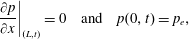 $$\begin{eqnarray}\displaystyle \left.\frac{\unicode[STIX]{x2202}p}{\unicode[STIX]{x2202}x}\right|_{(L,t)}=0\quad \text{and}\quad p(0,t)=p_{e}, & & \displaystyle\end{eqnarray}$$
where the parameters
 $h^{\ast }$
and
 $p_{e}$
represent the initial fracture aperture and the outlet pressure, respectively. Boundary condition (2.6b
) corresponds to an impervious boundary for the fluid at
 $x=L$
. The outlet pressure is a simplified representation of the external pressure against which the fracture is drained. For example, it may be considered as a hydrostatic head at the bottom of the fluid-filled well (borehole) where the fluid exits the fracture and flows to the surface. It may also represent a shut-in pressure (equilibrium pressure formed in a closed borehole).
2.2 Non-dimensionalization
We now define dimensionless variables by
 $$\begin{eqnarray}\displaystyle X=x/L,\quad H=h/h^{\ast },\quad P=(p-p_{e})/p_{c}\quad \text{and}\quad T=t/t_{c}, & & \displaystyle\end{eqnarray}$$
where
 $L$
and
 $h^{\ast }$
are the fracture’s initial dimensions and the characteristic scales for pressure and time are defined respectively by
 $$\begin{eqnarray}\displaystyle p_{c}=\hat{E}h^{\ast }\quad \text{and}\quad t_{c}=\frac{12\unicode[STIX]{x1D707}L^{2}}{\hat{E}{h^{\ast }}^{3}}. & & \displaystyle\end{eqnarray}$$
The governing equations (2.4) and (2.5) become
 $$\begin{eqnarray}\displaystyle & \displaystyle \frac{1}{H^{3}(T)}\frac{\text{d}H(T)}{\text{d}T}=\frac{\unicode[STIX]{x2202}^{2}P(X,T)}{\unicode[STIX]{x2202}X^{2}}, & \displaystyle\end{eqnarray}$$
 $$\begin{eqnarray}\displaystyle & \displaystyle \int _{0}^{1}P(X,T)\,\text{d}X=H(T)-P_{e}, & \displaystyle\end{eqnarray}$$
 $P_{e}=p_{e}/p_{c}$
. In addition, the initial and boundary conditions become
 $$\begin{eqnarray}\displaystyle H(0)=1, & & \displaystyle\end{eqnarray}$$
 $$\begin{eqnarray}\displaystyle \left.\frac{\unicode[STIX]{x2202}P}{\unicode[STIX]{x2202}X}\right|_{(1,T)}=0\quad \text{and}\quad P(0,T)=0. & & \displaystyle\end{eqnarray}$$
2.3 Solution
Now, we solve the dimensionless system (2.9), subject to the dimensionless initial and boundary conditions (2.10), and obtain the time and space evolution of the fracture aperture
 $H(T)$
and pressure
 $P(X,T)$
during the backflow process.
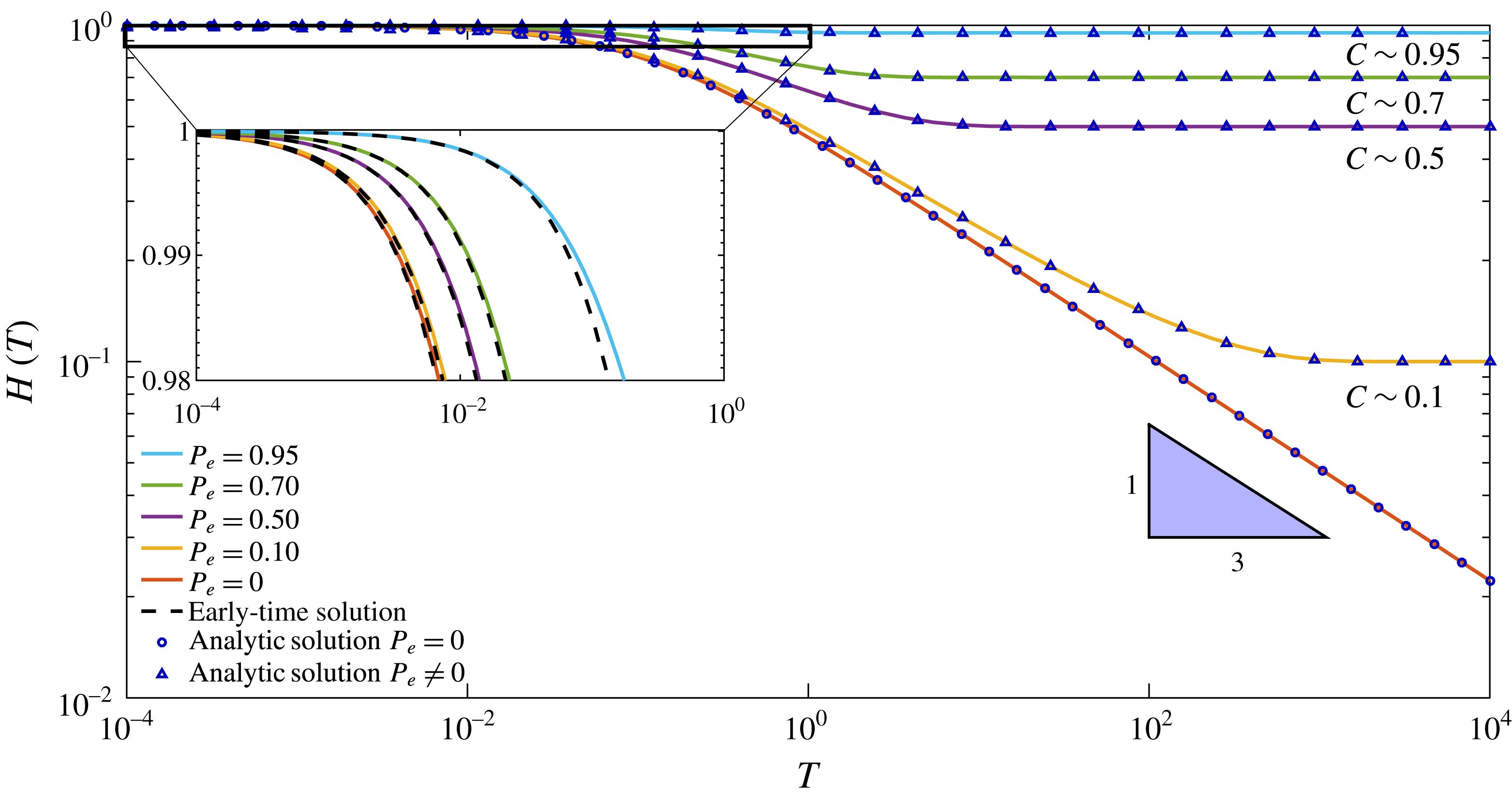
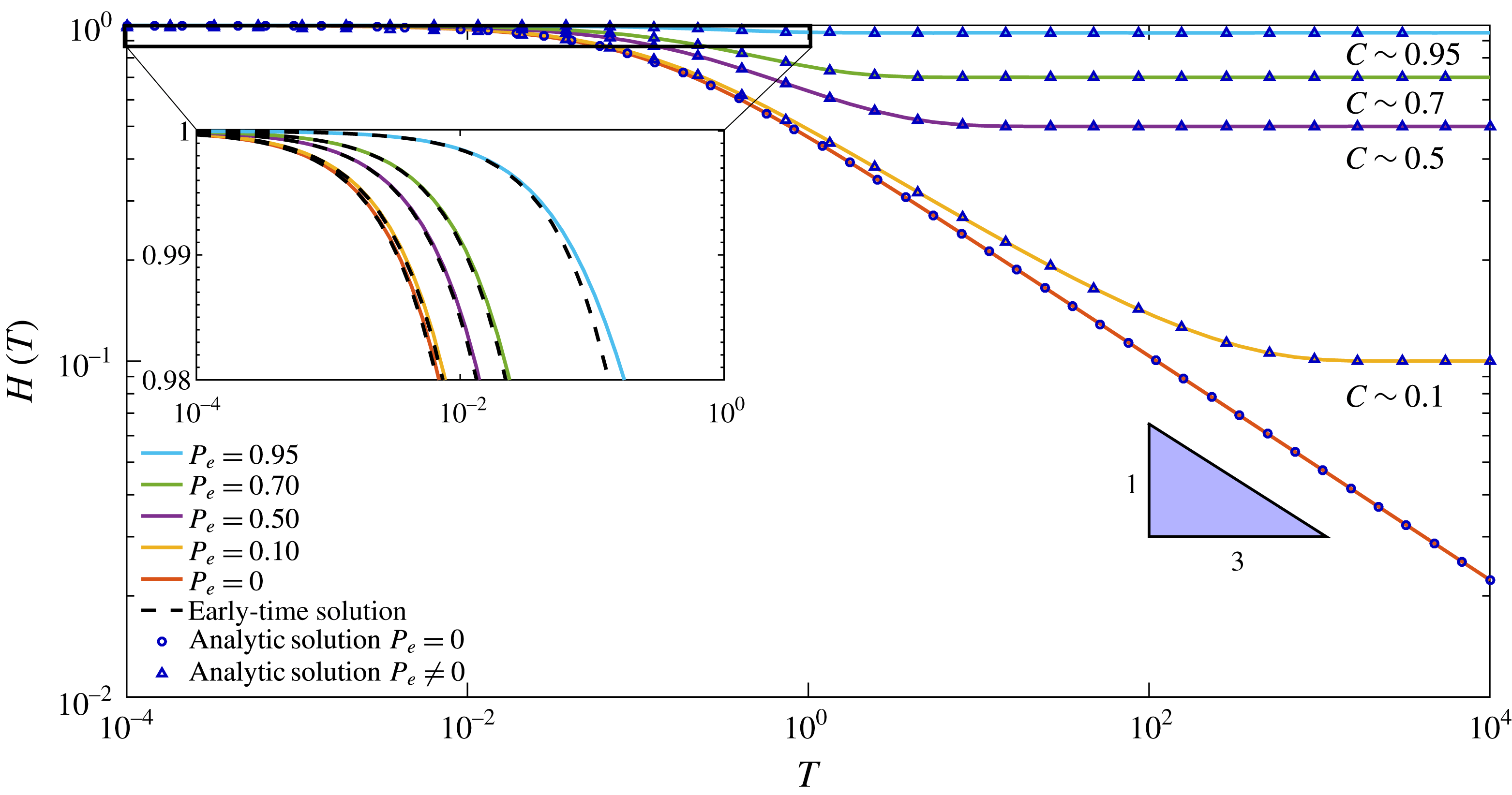
Numerical and analytic solutions for different values of
 $P_{e}$
. At late times (i.e.
 $T\gg 1$
) the solution tends asymptotically to a constant value
 $C=P_{e}$
. For
 $P_{e}=0$
, at late times, both the analytical and numerical solutions tend to a slope of
 $-1/3$
in the log–log plot.
Since
 $H$
is solely a function of
 $T$
, so is the left-hand side of (2.9a
). We therefore define
 $$\begin{eqnarray}\displaystyle G(T)=\frac{1}{H^{3}(T)}\frac{\text{d}H(T)}{\text{d}T}. & & \displaystyle\end{eqnarray}$$
Substituting (2.11) into (2.9a ), we obtain
 $$\begin{eqnarray}\displaystyle \frac{\unicode[STIX]{x2202}^{2}P(X,T)}{\unicode[STIX]{x2202}X^{2}}=G(T). & & \displaystyle\end{eqnarray}$$
Solving (2.12) using (2.10b,c ), we obtain
 $$\begin{eqnarray}\displaystyle P(X,T)=\left(\frac{X^{2}}{2}-X\right)G(T). & & \displaystyle\end{eqnarray}$$
Finally, we substitute (2.13) and (2.11) into (2.9b
) to obtain a first-order nonlinear ordinary differential equation (ODE) for
 $H(T)$
,
 $$\begin{eqnarray}\displaystyle -\frac{1}{3H^{3}(T)}\frac{\text{d}H(T)}{\text{d}T}=H(T)-P_{e}. & & \displaystyle\end{eqnarray}$$
In order to obtain a solution for (2.14) we discuss two cases: (I)
 $P_{e}=0$
; and (II)
 $P_{e}\neq 0$
, meaning that the fluid backflows against a known borehole pressure.
2.3.1 Case I:
 $P_{e}=0$

The case where
 $P_{e}$
vanishes allows us to solve the first-order ODE (2.14) for which the following simple analytic solution satisfying initial condition (2.10a
) exists:
 $$\begin{eqnarray}\displaystyle H(T)=(1+9T)^{-1/3}. & & \displaystyle\end{eqnarray}$$
The corresponding pressure distribution is
 $$\begin{eqnarray}\displaystyle P(X,T)={\textstyle \frac{3}{2}}(2X-X^{2})(1+9T)^{-1/3}. & & \displaystyle\end{eqnarray}$$
Although the solutions (2.15) and (2.16) are already in a simple form, we note that they can be approximated in the late-time limit,
 $T\gg 1$
, as
 $$\begin{eqnarray}\displaystyle & \displaystyle H(T)\sim (9T)^{-1/3}, & \displaystyle\end{eqnarray}$$
 $$\begin{eqnarray}\displaystyle & \displaystyle P(X,T)\sim {\textstyle \frac{3}{2}}(2X-X^{2})(9T)^{-1/3}. & \displaystyle\end{eqnarray}$$
 $H(T)$
and
 $P(X,T)$
are shown in figures 2 and 3. We also note that the case where
 $P_{e}=0$
is a singular limit with
 $H(T)$
tending towards zero. As we shall see, the
 $T^{-1/3}$
behaviour of
 $H$
and
 $P$
is also seen for the more complicated networks discussed in §§ 3 and 4.
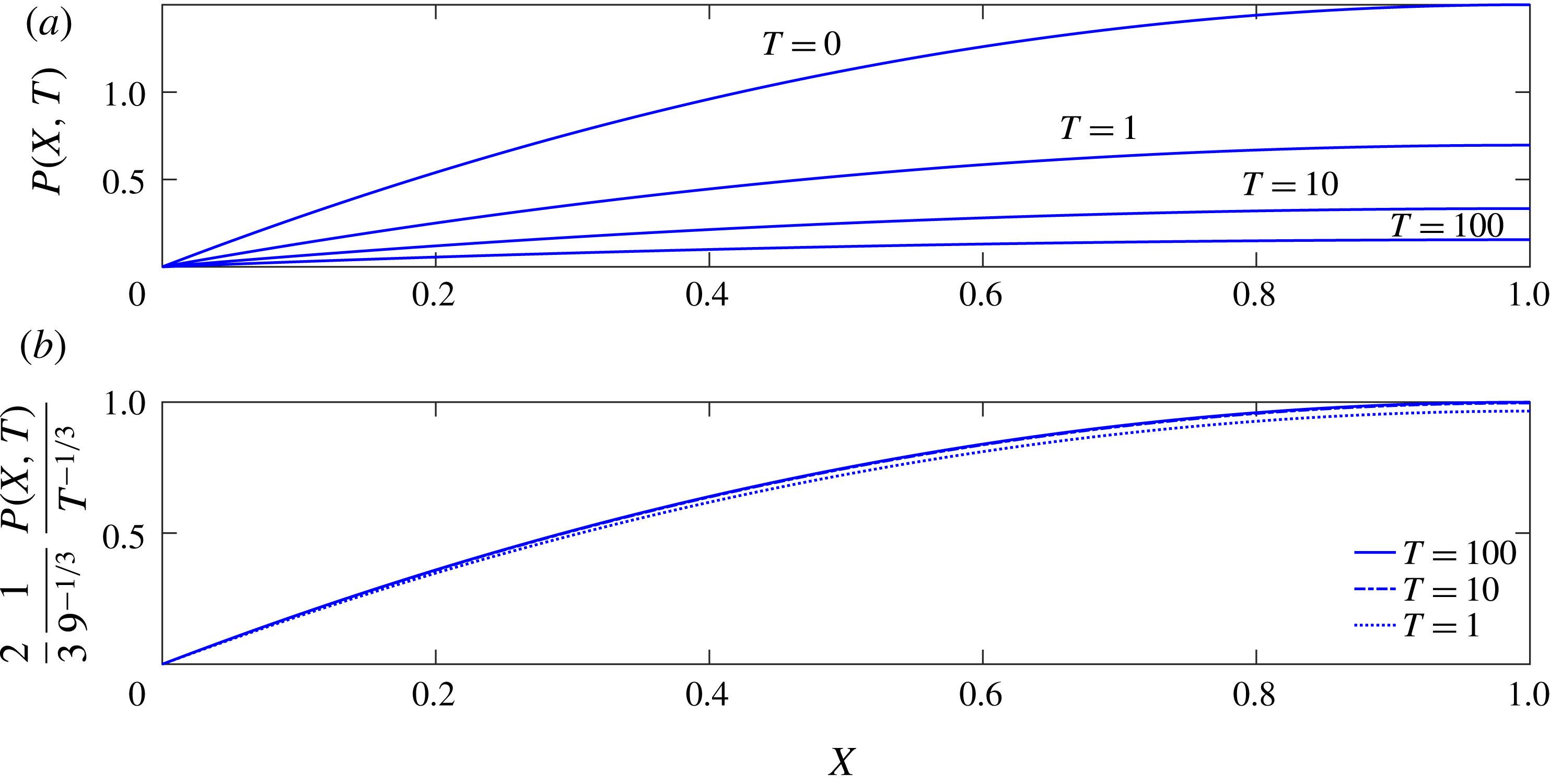
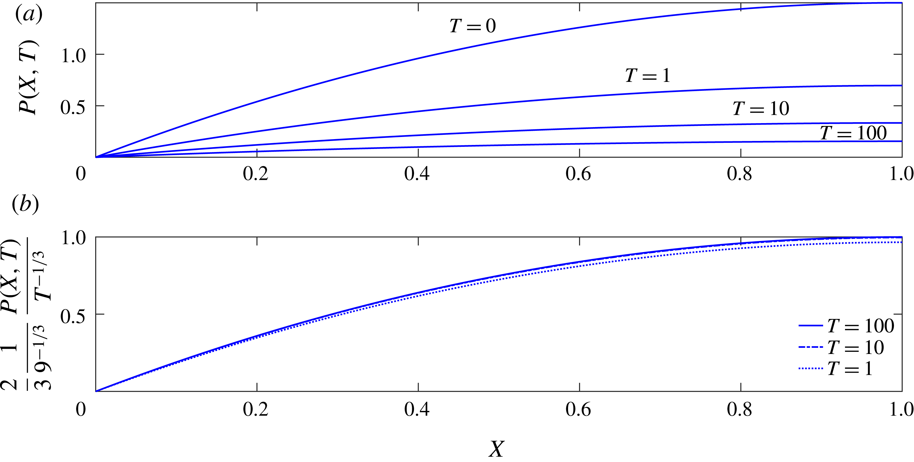
Numerical results for a single fracture with outlet pressure
 $P_{e}=0$
. (a) Non-dimensional pressure distribution (2.16) within the fracture at different times. As time increases, the pressure at the crack tip (i.e.
 $X=1$
) decreases and the pressure profile flattens. (b) When rescaled by
 $T^{-1/3}$
, the late-time pressure distribution tends towards a universal curve.
2.3.2 Case II:
$P_{e}\neq 0$

The case where
 $P_{e}\neq 0$
leaves us with the non-homogeneous, nonlinear ODE (2.14). Integration using (2.10a
) yields an implicit equation for
 $H(T)$
,
 $$\begin{eqnarray}\displaystyle \ln \left(\frac{H(T)(1-P_{e})}{H(T)-P_{e}}\right)-\frac{P_{e}}{H(T)}-\frac{1}{2}\left(\frac{P_{e}}{H(T)}\right)^{2}+P_{e}+\frac{1}{2}P_{e}^{2}-3P_{e}^{3}T=0. & & \displaystyle\end{eqnarray}$$
Since (2.18) typically requires a numerical solution, we proceed to calculate explicit approximations for
 $H(T)$
at early and late times. For early times (
 $T\ll 1$
), we substitute
 $$\begin{eqnarray}\displaystyle H(T)=1-f(T),\quad f(T)\ll 1, & & \displaystyle\end{eqnarray}$$
into (2.18) and use Taylor expansion to obtain the leading-order result
 $f(T)\sim 3(1-P_{e})T$
and hence
 $$\begin{eqnarray}\displaystyle & \displaystyle H(T)\sim 1-3(1-P_{e})T, & \displaystyle\end{eqnarray}$$
 $$\begin{eqnarray}\displaystyle & \displaystyle P(X,T)\sim {\textstyle \frac{3}{2}}(2X-X^{2})(1-P_{e}). & \displaystyle\end{eqnarray}$$
 $T\gg 1$
, we expect
 $H(T)$
to approach
 $P_{e}$
and hence substitute
 $$\begin{eqnarray}\displaystyle H(T)=P_{e}+g(T),\quad g(T)\ll P_{e}, & & \displaystyle\end{eqnarray}$$
into (2.18) to find
 $$\begin{eqnarray}\displaystyle & \displaystyle H(T)\sim P_{e}+P_{e}(1-P_{e})\text{e}^{-3P_{e}^{3}T}, & \displaystyle\end{eqnarray}$$
 $$\begin{eqnarray}\displaystyle & \displaystyle P(X,T)\sim {\textstyle \frac{3}{2}}(2X-X^{2})P_{e}(1-P_{e})\text{e}^{-3P_{e}^{3}T}. & \displaystyle\end{eqnarray}$$
Numerical simulation of (2.14) was performed using the Matlab subroutine ‘ODE15s’. The implicit equation (2.18) was solved using the Matlab subroutine ‘fsolve’. Five numerical solutions were obtained using different
 $P_{e}$
values, and a comparison was made between the analytic solutions (2.15), (2.18) and (2.20a
) and the numerical results, as seen in figure 2. The good agreement gives us confidence that our numerical method works when moving to more complex networks. We note that the value of
 $P_{e}$
is assumed to be in the range of
 $[0,1]$
:
 $P_{e}=0$
is the previous case solved analytically, and
 $P_{e}=1$
signifies a bounded value for the borehole pressure. Above it, outward flow cannot occur and the fracture would grow instead of relaxing.
Results for the numerical simulation are presented in figure 2, and illustrate that at late times (or equilibrium) the solutions asymptotically tend towards a constant
 $C=P_{e}$
. In order to validate the numerical simulation, the analytic solutions are plotted against the numerical simulation, as well as early-time asymptotic approximations for the different
 $P_{e}$
values.
The space and time evolution of pressure for the single-fracture model with
 $P_{e}=0$
is presented in figure 3(a). The pressure profile was calculated at four dimensionless times
 $T=\{0,1,10,100\}$
. As time increases, the pressure at the tip,
 $X=1$
, decreases and the profile flattens. Figure 3(b) shows that scaling the pressure by
 $T^{-1/3}$
collapses the distribution into a single universal curve that retains its shape over time.
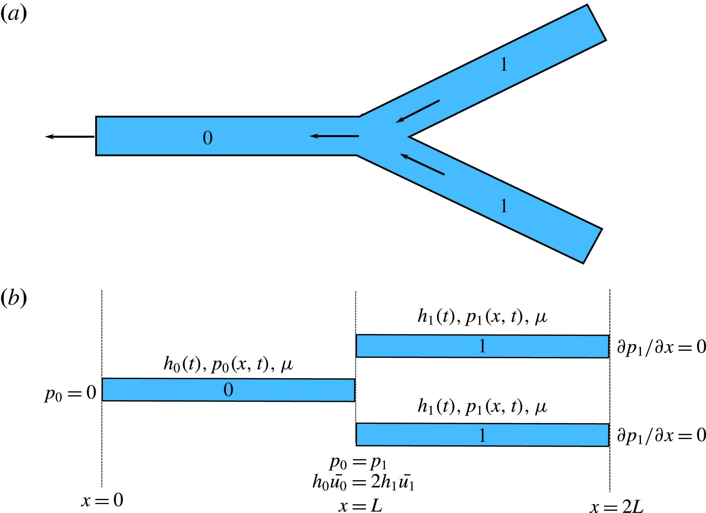
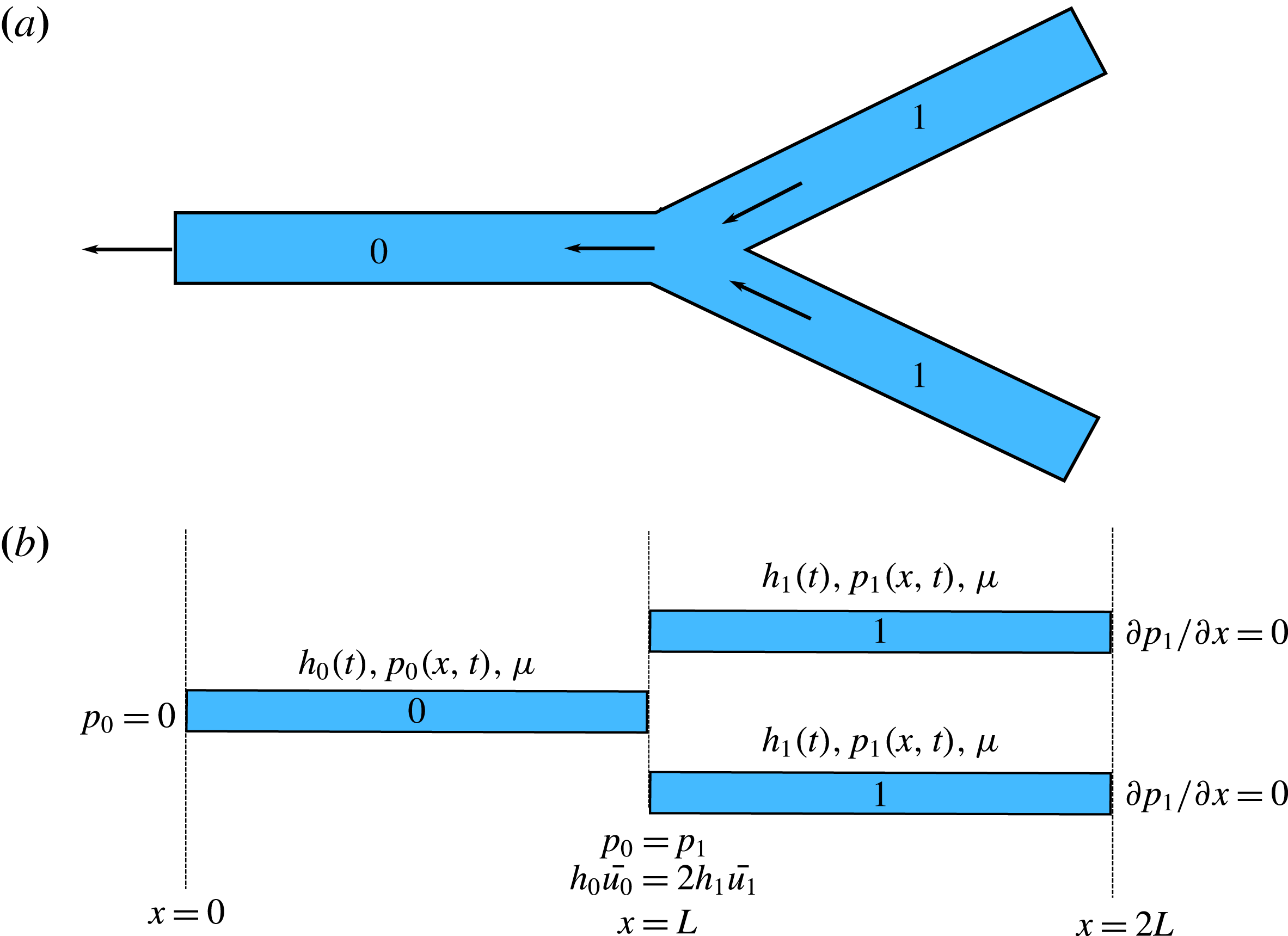
(a) A schematic representation of a bifurcated model fracture network. (b) Our mathematical model of the bifurcated fracture network is formulated as a series of connected one-dimensional fractures, while ignoring the angle and end effects. The variables and boundary conditions are also presented.
3 A simple fracture network: a bifurcated channel
We now continue by using a similar problem formulation for a model fracture network, resolving not only the relaxation dynamics of a single fracture but also the dynamics of a system of connected fractures. As before, the fracture apertures are assumed to depend only on time. For that purpose we suggest a simple model using a bifurcated channel, i.e. a single junction between three fractures as shown in figure 4(a). The three elastic channels are numbered, ‘0’ for the outlet channel and ‘1’ for the identical back channels.
3.1 Governing equations
The three-fracture system includes a total of four variables: the pressure distributions within the fractures,
 $p_{0}(x,t)$
and
 $p_{1}(x,t)$
, and apertures
 $h_{0}(t)$
and
 $h_{1}(t)$
. The governing equations include two equations for each of the fracture apertures
 $$\begin{eqnarray}\displaystyle & \displaystyle \frac{\text{d}h_{0}(t)}{\text{d}t}=\frac{h_{0}^{3}(t)}{12\unicode[STIX]{x1D707}}\frac{\unicode[STIX]{x2202}^{2}p_{0}(x,t)}{\unicode[STIX]{x2202}x^{2}}, & \displaystyle\end{eqnarray}$$
 $$\begin{eqnarray}\displaystyle & \displaystyle \frac{\text{d}h_{1}(t)}{\text{d}t}=\frac{h_{1}^{3}(t)}{12\unicode[STIX]{x1D707}}\frac{\unicode[STIX]{x2202}^{2}p_{1}(x,t)}{\unicode[STIX]{x2202}x^{2}}, & \displaystyle\end{eqnarray}$$
 $$\begin{eqnarray}\displaystyle & \displaystyle \int _{0}^{L}p_{0}(x,t)\,\text{d}x=\hat{E}Lh_{0}(t), & \displaystyle\end{eqnarray}$$
 $$\begin{eqnarray}\displaystyle & \displaystyle \int _{L}^{2L}p_{1}(x,t)\,\text{d}x=\hat{E}Lh_{1}(t). & \displaystyle\end{eqnarray}$$
 $h_{0}(t)$
and
 $h_{1}(t)$
and two boundary conditions for the pressure distributions
 $p_{0}(x,t)$
and
 $p_{1}(x,t)$
in each of the fractures. The initial conditions are given by
 $$\begin{eqnarray}\displaystyle h_{0}(0)=h_{1}(0)=h^{\ast }, & & \displaystyle\end{eqnarray}$$
and the boundary conditions are
 $$\begin{eqnarray}\displaystyle & \displaystyle p_{0}(0,t)=0, & \displaystyle\end{eqnarray}$$
 $$\begin{eqnarray}\displaystyle & \displaystyle p_{0}(L,t)=p_{1}(L,t), & \displaystyle\end{eqnarray}$$
 $$\begin{eqnarray}\displaystyle & \displaystyle h_{0}^{3}\left.\frac{\unicode[STIX]{x2202}p_{0}}{\unicode[STIX]{x2202}x}\right|_{(L,t)}=2h_{1}^{3}\left.\frac{\unicode[STIX]{x2202}p_{1}}{\unicode[STIX]{x2202}x}\right|_{(L,t)}, & \displaystyle\end{eqnarray}$$
 $$\begin{eqnarray}\displaystyle & \displaystyle \left.\frac{\unicode[STIX]{x2202}p_{1}}{\unicode[STIX]{x2202}x}\right|_{(2L,t)}=0. & \displaystyle\end{eqnarray}$$
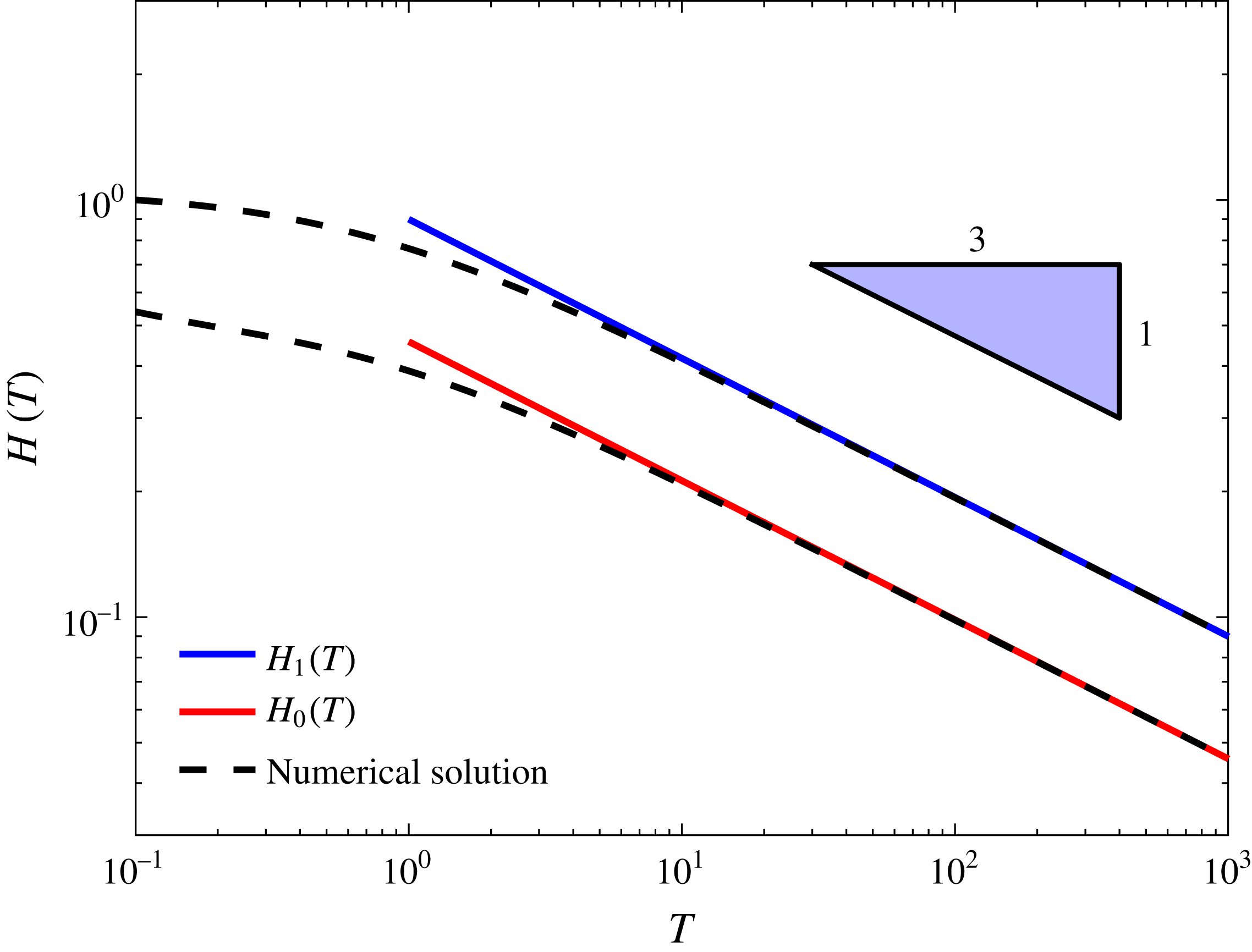
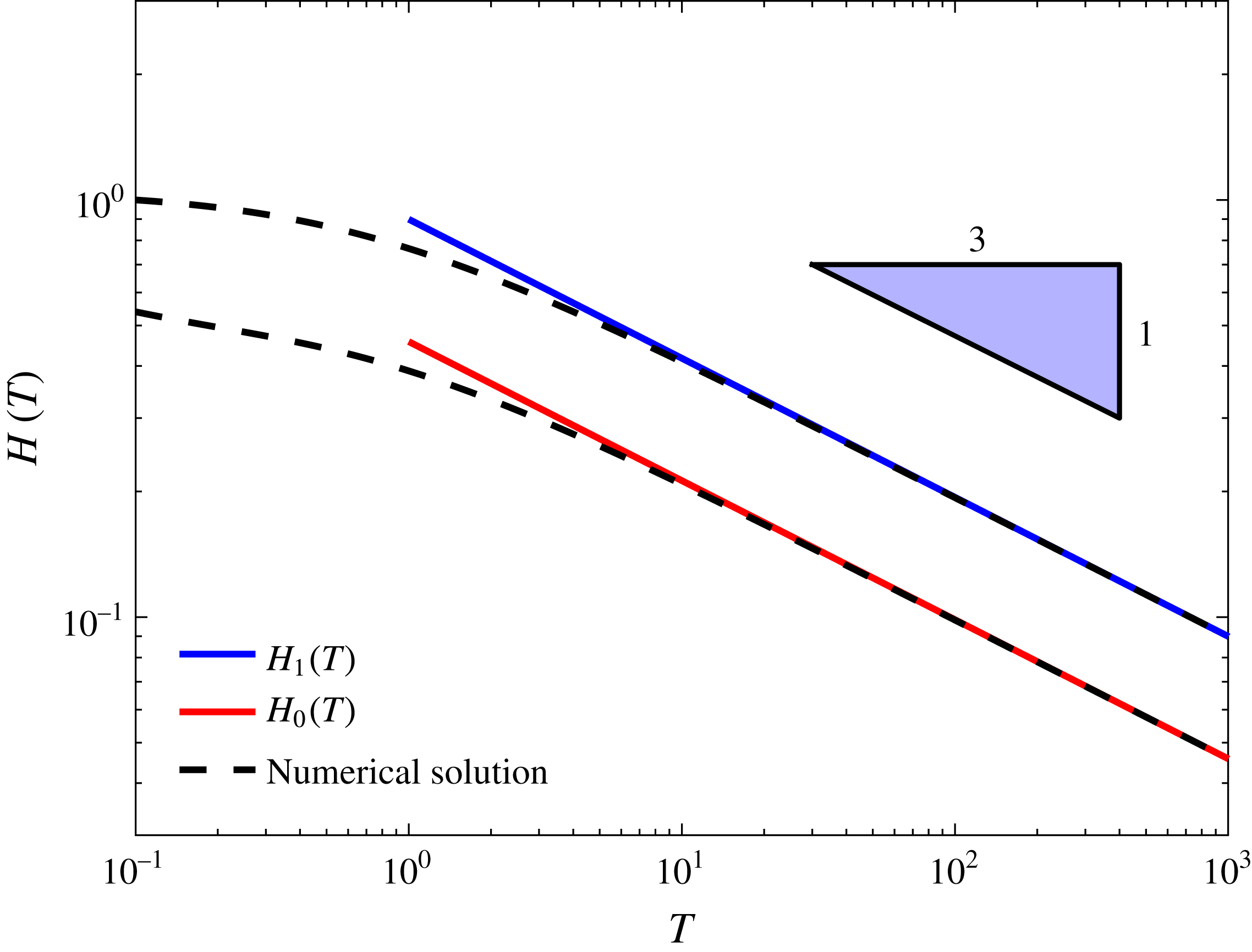
Time evolution of fracture apertures
 $H_{1}(T)$
and
 $H_{2}(T)$
: numerical solutions versus late-time asymptotic solutions. Both solutions for
 $H_{1}(T)$
and
 $H_{2}(T)$
show a slope of
 $-1/3$
at late times.
3.2 Non-dimensionalization
The dimensionless variables are introduced as
 $$\begin{eqnarray}\displaystyle X=x/2L,\quad H_{0}=h_{0}/h^{\ast },\quad H_{1}=h_{1}/h^{\ast },\quad P_{0}=p_{0}/p_{c},\quad P_{1}=p_{1}/p_{c}\quad \text{and}\quad T=t/t_{c}, & & \displaystyle \nonumber\\ \displaystyle & & \displaystyle\end{eqnarray}$$
where the characteristic scales for pressure and time are now
 $$\begin{eqnarray}\displaystyle p_{c}=\frac{\hat{E}h^{\ast }}{2}\quad \text{and}\quad t_{c}=\frac{96\unicode[STIX]{x1D707}L^{2}}{\hat{E}{h^{\ast }}^{3}}. & & \displaystyle\end{eqnarray}$$
In dimensionless form the governing differential equations are
 $$\begin{eqnarray}\displaystyle & \displaystyle \frac{1}{H_{0}^{3}(T)}\frac{\text{d}H_{0}(T)}{\text{d}T}=\frac{\unicode[STIX]{x2202}^{2}P_{0}(X,T)}{\unicode[STIX]{x2202}X^{2}}, & \displaystyle\end{eqnarray}$$
 $$\begin{eqnarray}\displaystyle & \displaystyle \frac{1}{H_{1}^{3}(T)}\frac{\text{d}H_{1}(T)}{\text{d}T}=\frac{\unicode[STIX]{x2202}^{2}P_{1}(X,T)}{\unicode[STIX]{x2202}X^{2}}, & \displaystyle\end{eqnarray}$$
 $$\begin{eqnarray}\displaystyle & \displaystyle \int _{0}^{1/2}P_{0}(X,T)\,\text{d}X=H_{0}(T), & \displaystyle\end{eqnarray}$$
 $$\begin{eqnarray}\displaystyle & \displaystyle \int _{1/2}^{1}P_{1}(X,T)\,\text{d}X=H_{1}(T). & \displaystyle\end{eqnarray}$$
 $$\begin{eqnarray}\displaystyle & \displaystyle H_{0}(0)=1, & \displaystyle\end{eqnarray}$$
 $$\begin{eqnarray}\displaystyle & \displaystyle H_{1}(0)=1, & \displaystyle\end{eqnarray}$$
 $$\begin{eqnarray}\displaystyle & \displaystyle P_{0}(0,T)=0, & \displaystyle\end{eqnarray}$$
 $$\begin{eqnarray}\displaystyle & \displaystyle P_{0}\left({\textstyle \frac{1}{2}},T\right)=P_{1}\left({\textstyle \frac{1}{2}},T\right), & \displaystyle\end{eqnarray}$$
 $$\begin{eqnarray}\displaystyle & \displaystyle H_{0}^{3}\left.\frac{\unicode[STIX]{x2202}P_{0}}{\unicode[STIX]{x2202}X}\right|_{(1/2,T)}=2H_{1}^{3}\left.\frac{\unicode[STIX]{x2202}P_{1}}{\unicode[STIX]{x2202}X}\right|_{(1/2,T)}, & \displaystyle\end{eqnarray}$$
 $$\begin{eqnarray}\displaystyle & \displaystyle \left.\frac{\unicode[STIX]{x2202}P_{1}}{\unicode[STIX]{x2202}X}\right|_{(1,T)}=0. & \displaystyle\end{eqnarray}$$
 $H_{0}(T)$
and
 $H_{1}(T)$
and pressure distributions
 $P_{0}(X,T)$
and
 $P_{1}(X,T)$
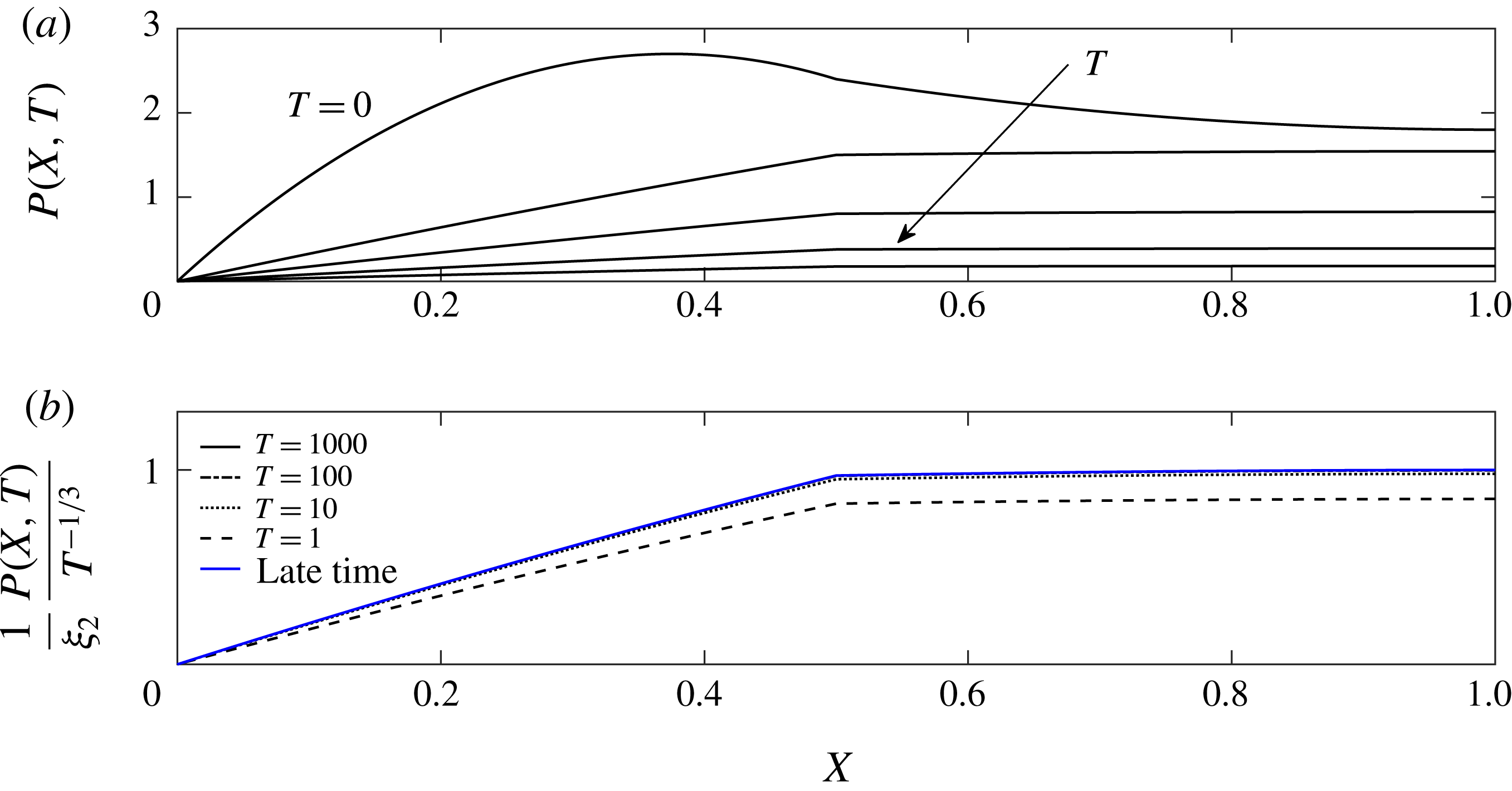
, as shown in figures 5 and 6(a). We seek analytical insight for late times in the following section (see appendix A for details about the numerical method).
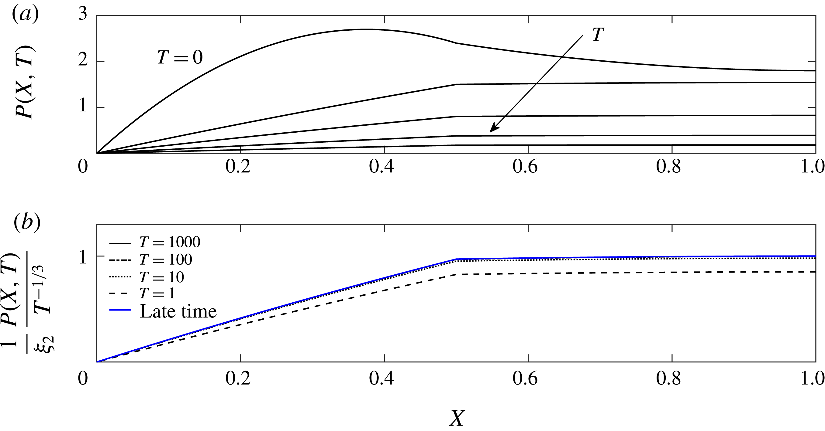
Time evolution of the non-dimensional pressure distribution within the fracture network: (a) raw numerical data at
 $T=\{0,1,10,100,1000\}$
, and (b) rescaled numerical data. In (b) we also plot the asymptotic solution (3.16) at late times. The rescaled numerical data approach the asymptotic solution as time progresses.
3.3 Late-time asymptotic solutions
Inspired by the results for a single fracture, we seek a late-time solution in which the apertures and pressures decay as
 $T^{-1/3}$
. (This can also be justified by a scaling analysis of the governing equations (3.7)–(3.9).) Hence, we make the ansatz
 $$\begin{eqnarray}\displaystyle H_{i}(T)={\hat{H}}_{i}T^{-1/3},\quad P_{i}(X,T)=\hat{P}_{i}(X)T^{-1/3}, & & \displaystyle\end{eqnarray}$$
and solve for
 ${\hat{H}}_{i}$
and
 $\hat{P}_{i}$
(where
 $i=0,1$
).
The governing equations (3.7) can be integrated to yield
 $$\begin{eqnarray}\displaystyle \hat{P}_{0}(X)=-\frac{1}{3{\hat{H}}_{0}^{2}}\left(\frac{1}{2}X^{2}+a_{1}X+a_{2}\right),\quad \hat{P}_{1}(X)=-\frac{1}{3{\hat{H}}_{1}^{2}}\left(\frac{1}{2}X^{2}+b_{1}X+b_{2}\right). & & \displaystyle\end{eqnarray}$$
Substituting (3.11) into the force balances (3.8), we derive
 $$\begin{eqnarray}\displaystyle \frac{1}{3{\hat{H}}_{0}^{3}}\left(\frac{1}{48}+\frac{1}{8}a_{1}+\frac{1}{2}a_{2}\right)=-1,\quad \frac{1}{3{\hat{H}}_{1}^{3}}\left(\frac{7}{48}+\frac{3}{8}b_{1}+\frac{1}{2}b_{2}\right)=-1, & & \displaystyle\end{eqnarray}$$
which yields
 $$\begin{eqnarray}\displaystyle {\hat{H}}_{0}=\bigg(\frac{-3}{\frac{1}{48}+\frac{1}{8}a_{1}+\frac{1}{2}a_{2}}\bigg)^{-1/3},\quad {\hat{H}}_{1}=\bigg(\frac{-3}{\frac{7}{48}+\frac{3}{8}b_{1}+\frac{1}{2}b_{2}}\bigg)^{-1/3}. & & \displaystyle\end{eqnarray}$$
In order to achieve a solution we must now find the values of the integration constants. Substituting (3.13a,b
) into boundary condition (3.9c
,
f
) we obtain that
 $a_{2}=0$
and
 $b_{1}=-1$
respectively. Substituting (3.11) and (3.13) into the boundary conditions (3.9d
,
e
), we achieve a set of two nonlinear equations for two unknowns. The nonlinear system was solved numerically using Mathematica’s subroutine ‘NSolve’ to yield
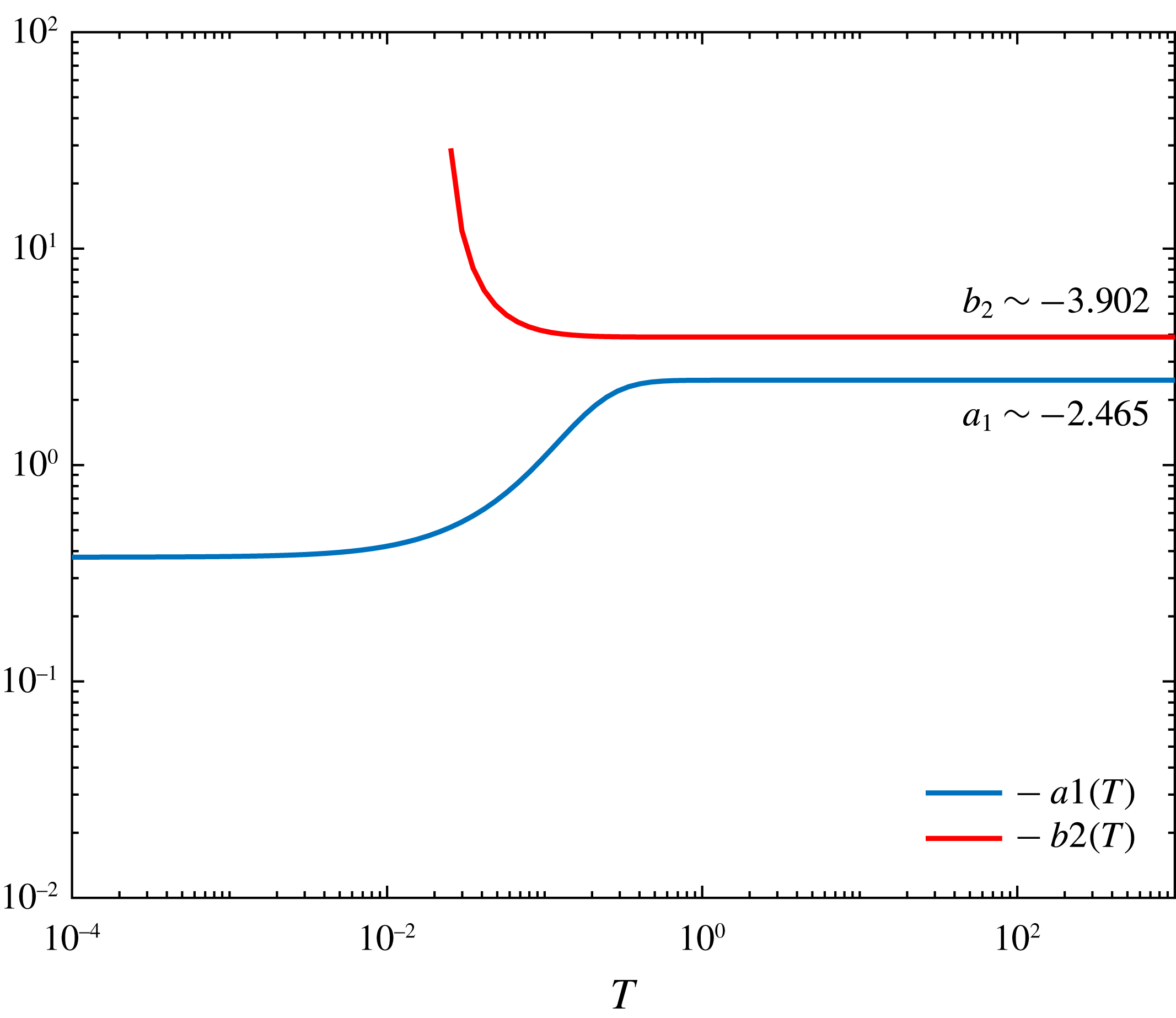
 $$\begin{eqnarray}\displaystyle a_{1}\approx -2.4650\quad \text{and}\quad b_{2}\approx -3.9016. & & \displaystyle\end{eqnarray}$$
The late-time asymptotic solutions for
 $H_{0}(T)$
and
 $H_{1}(T)$
are thus
 $$\begin{eqnarray}\displaystyle & \displaystyle H_{0}(T)\sim {\hat{H}}_{0}T^{-1/3}=0.4575\,T^{-1/3}, & \displaystyle\end{eqnarray}$$
 $$\begin{eqnarray}\displaystyle & \displaystyle H_{1}(T)\sim {\hat{H}}_{1}T^{-1/3}=0.8990\,T^{-1/3}, & \displaystyle\end{eqnarray}$$
 $$\begin{eqnarray}\displaystyle & \displaystyle P_{0}(X,T)\sim \hat{P}_{0}(X)T^{-1/3}=1.764(2.226X-0.451X^{2})\,T^{-1/3}, & \displaystyle\end{eqnarray}$$
 $$\begin{eqnarray}\displaystyle & \displaystyle P_{1}(X,T)\sim \hat{P}_{1}(X)T^{-1/3}=1.815(0.886+0.227X-0.113X^{2})\,T^{-1/3}, & \displaystyle\end{eqnarray}$$
 $\unicode[STIX]{x1D709}_{2}=\hat{P}_{1}(1)=1.815$
as the coefficient of the pressure at the network tip (
 $X=1$
).
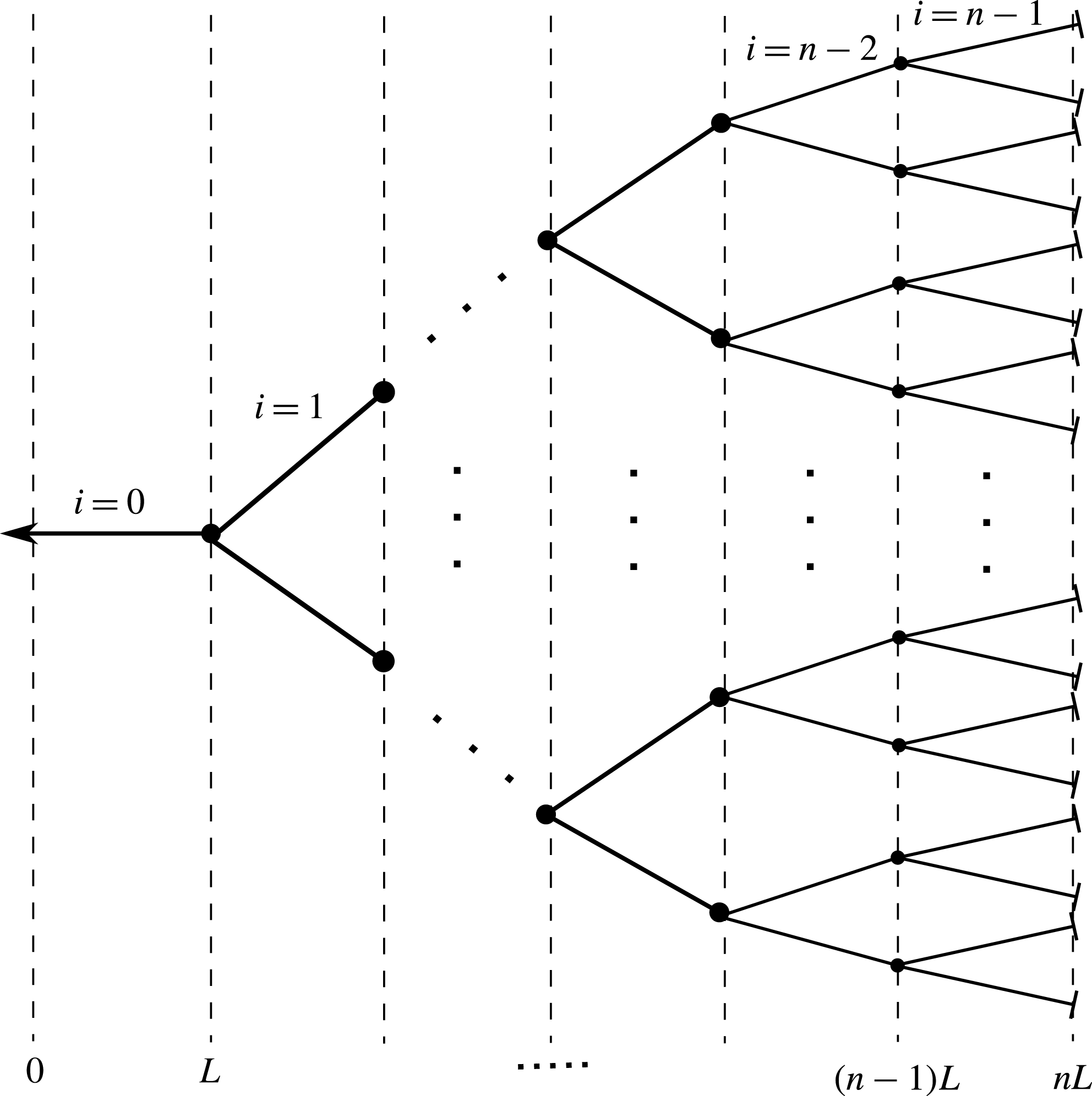
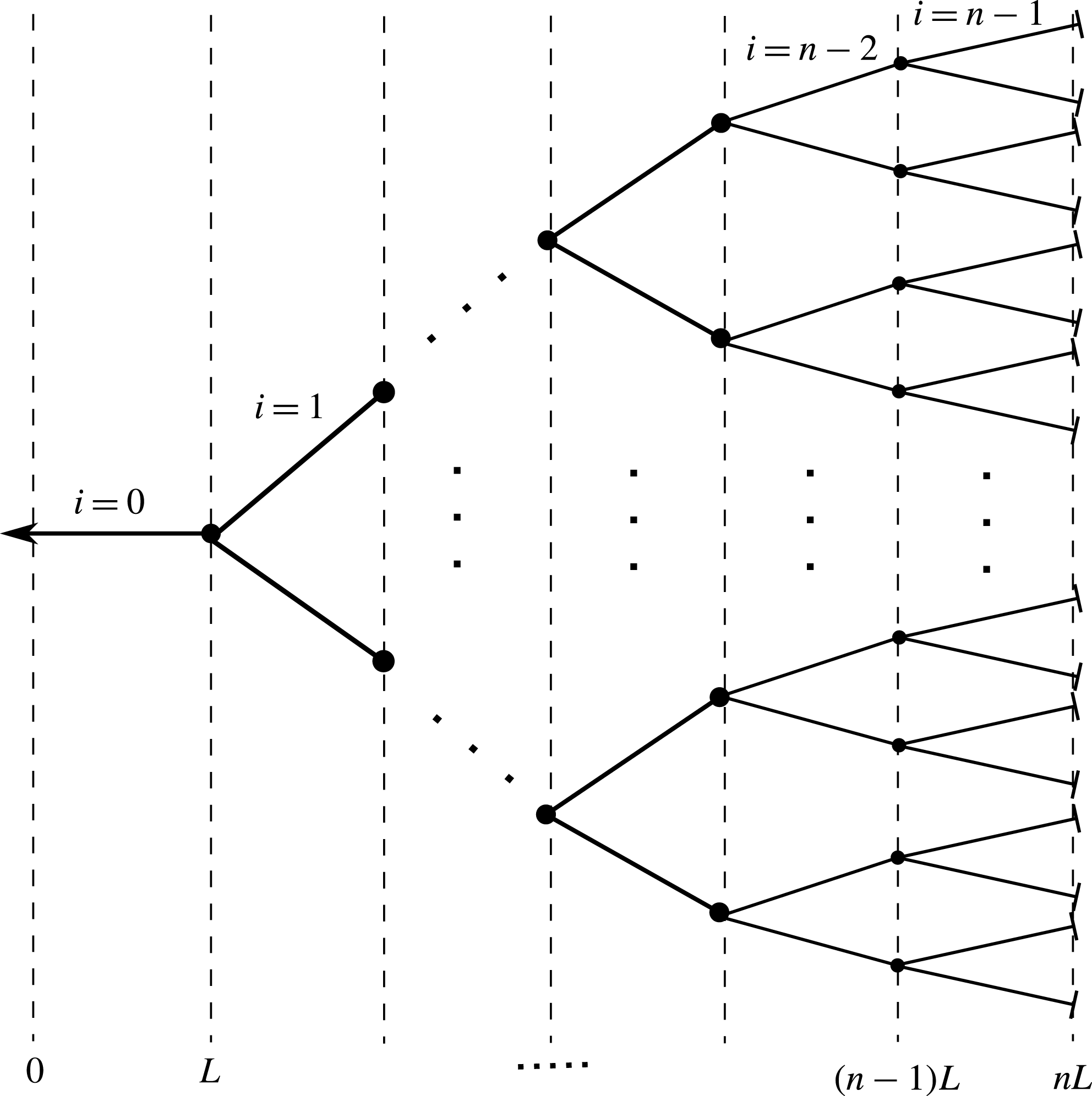
A model bifurcating fracture network of
 $n$
generations.
4 Generalization of a fracture network
We now proceed to further generalize our problem to the case of a multi-bifurcated network composed of
 $n$
fractures of length
 $L$
in a row, with a total of
 $2^{n-1}-1$
junctions and
 $2^{n}-1$
channels, as shown in figure 7. The channels are indexed using
 $i=0,1,2,\ldots ,n-1$
where
 $i=0$
is the outer channel with the outlet located at
 $x=0$
and
 $i=n-1$
is the innermost fracture with its tip at
 $x=nL$
.
4.1 Governing equations
The problem formulation remains similar to that in § 3 with an increased number of variables and initial and boundary conditions. The governing equations for each fracture are again
 $$\begin{eqnarray}\displaystyle & \displaystyle \frac{12\unicode[STIX]{x1D707}}{h_{i}^{3}(t)}\frac{\text{d}h_{i}(t)}{\text{d}t}=\frac{\unicode[STIX]{x2202}^{2}p_{i}(x,t)}{\unicode[STIX]{x2202}x^{2}},\quad \text{where }i=0,1,\ldots ,n-1, & \displaystyle\end{eqnarray}$$
 $$\begin{eqnarray}\displaystyle & \displaystyle \int _{iL}^{(i+1)L}p_{i}(x,t)\,\text{d}x=\hat{E}Lh_{i}(t),\quad \text{where }i=0,1,\ldots ,n-1. & \displaystyle\end{eqnarray}$$
 $2n$
equations and
 $2n$
unknowns. Since each equation requires an initial condition and two boundary conditions, we require a total of
 $n$
initial conditions and
 $2n$
boundary conditions in order to complete the problem. The initial and boundary conditions are given by
 $$\begin{eqnarray}\displaystyle & \displaystyle h_{i}(0)=h^{\ast },\quad \text{where}~i=0,1,\ldots ,n-1, & \displaystyle\end{eqnarray}$$
 $$\begin{eqnarray}\displaystyle & \displaystyle p_{0}(0,t)=0, & \displaystyle\end{eqnarray}$$
 $$\begin{eqnarray}\displaystyle & \displaystyle p_{i}(iL,t)=p_{i+1}(iL,t),\quad \text{where}~i=1,2,\ldots ,n-1, & \displaystyle\end{eqnarray}$$
 $$\begin{eqnarray}\displaystyle & \displaystyle h_{i}^{3}\left.\frac{\unicode[STIX]{x2202}p_{i}}{\unicode[STIX]{x2202}x}\right|_{(iL,t)}=2h_{i+1}^{3}\left.\frac{\unicode[STIX]{x2202}p_{i+1}}{\unicode[STIX]{x2202}x}\right|_{(iL,t)},\quad \text{where}~i=1,2,\ldots ,n-1, & \displaystyle\end{eqnarray}$$
 $$\begin{eqnarray}\displaystyle & \displaystyle \left.\frac{\unicode[STIX]{x2202}p_{n-1}}{\unicode[STIX]{x2202}x}\right|_{(nL,t)}=0. & \displaystyle\end{eqnarray}$$
4.2 Non-dimensionalization
We non-dimensionalize the system using
 $$\begin{eqnarray}\displaystyle X=x/nL,\quad H_{i}=h_{i}/h^{\ast }.\quad P_{i}=p_{i}/p_{c}\quad \text{and}\quad T=t/t_{c}, & & \displaystyle\end{eqnarray}$$
where the characteristic scales for pressure and time become
 $$\begin{eqnarray}\displaystyle p_{c}=\frac{\hat{E}h^{\ast }}{n}\quad \text{and}\quad t_{c}=\frac{12\unicode[STIX]{x1D707}n^{3}L^{2}}{\hat{E}{h^{\ast }}^{3}}. & & \displaystyle\end{eqnarray}$$
The resulting dimensionless equations are then
 $$\begin{eqnarray}\displaystyle & \displaystyle \frac{1}{H_{i}^{3}(T)}\frac{\text{d}H_{i}(T)}{\text{d}T}=\frac{\unicode[STIX]{x2202}^{2}P_{i}(X,T)}{\unicode[STIX]{x2202}X^{2}}, & \displaystyle\end{eqnarray}$$
 $$\begin{eqnarray}\displaystyle & \displaystyle \int _{i/n}^{(i+1)/n}P_{i}(X,T)\,\text{d}X=H_{i}(T),\quad \text{where }i=0,1,\ldots ,n-1, & \displaystyle\end{eqnarray}$$
 $$\begin{eqnarray}\displaystyle & \displaystyle H_{i}(0)=1,\quad \text{where}~i=0,1,\ldots ,n-1, & \displaystyle\end{eqnarray}$$
 $$\begin{eqnarray}\displaystyle & \displaystyle P_{0}(0,T)=0, & \displaystyle\end{eqnarray}$$
 $$\begin{eqnarray}\displaystyle & \displaystyle P_{i}(i/n,T)=P_{i+1}(i/n,T),\quad \text{where}~i=1,2,\ldots ,n-1, & \displaystyle\end{eqnarray}$$
 $$\begin{eqnarray}\displaystyle & \displaystyle H_{i}^{3}\left.\frac{\unicode[STIX]{x2202}P_{i}}{\unicode[STIX]{x2202}X}\right|_{(i/n,T)}=2H_{i+1}^{3}\left.\frac{\unicode[STIX]{x2202}P_{i+1}}{\unicode[STIX]{x2202}X}\right|_{(i/n,T)},\quad \text{where}~i=1,2,\ldots ,n-1, & \displaystyle\end{eqnarray}$$
 $$\begin{eqnarray}\displaystyle & \displaystyle \left.\frac{\unicode[STIX]{x2202}P_{n-1}}{\unicode[STIX]{x2202}X}\right|_{(1,T)}=0. & \displaystyle\end{eqnarray}$$
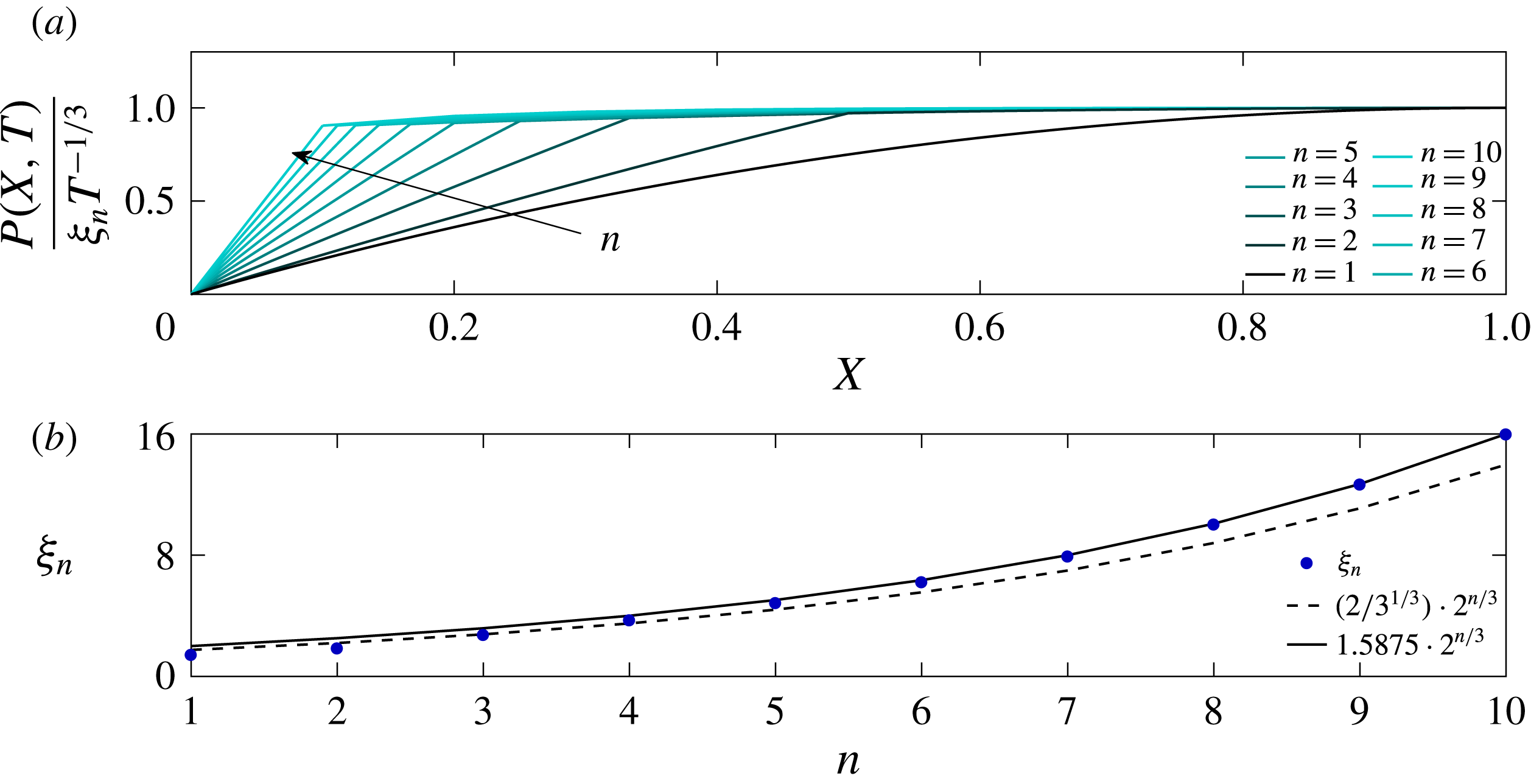
Systematic changes in the pressure distribution with increased number of generations
 $n$
: (a) pressure distribution within the fracture at
 $T\gg 1$
and (b) maximum pressure value as a function of
 $n$
.
(a) Non-dimensional flow rates from the network outlet at
 $X=1$
for different values of
 $n$
. At late time the curves tend to a negative slope of
 $-4/3$
. (b) Cumulative volume of rejected fluid from the network normalized by the initial volume of retained fluid in the network.
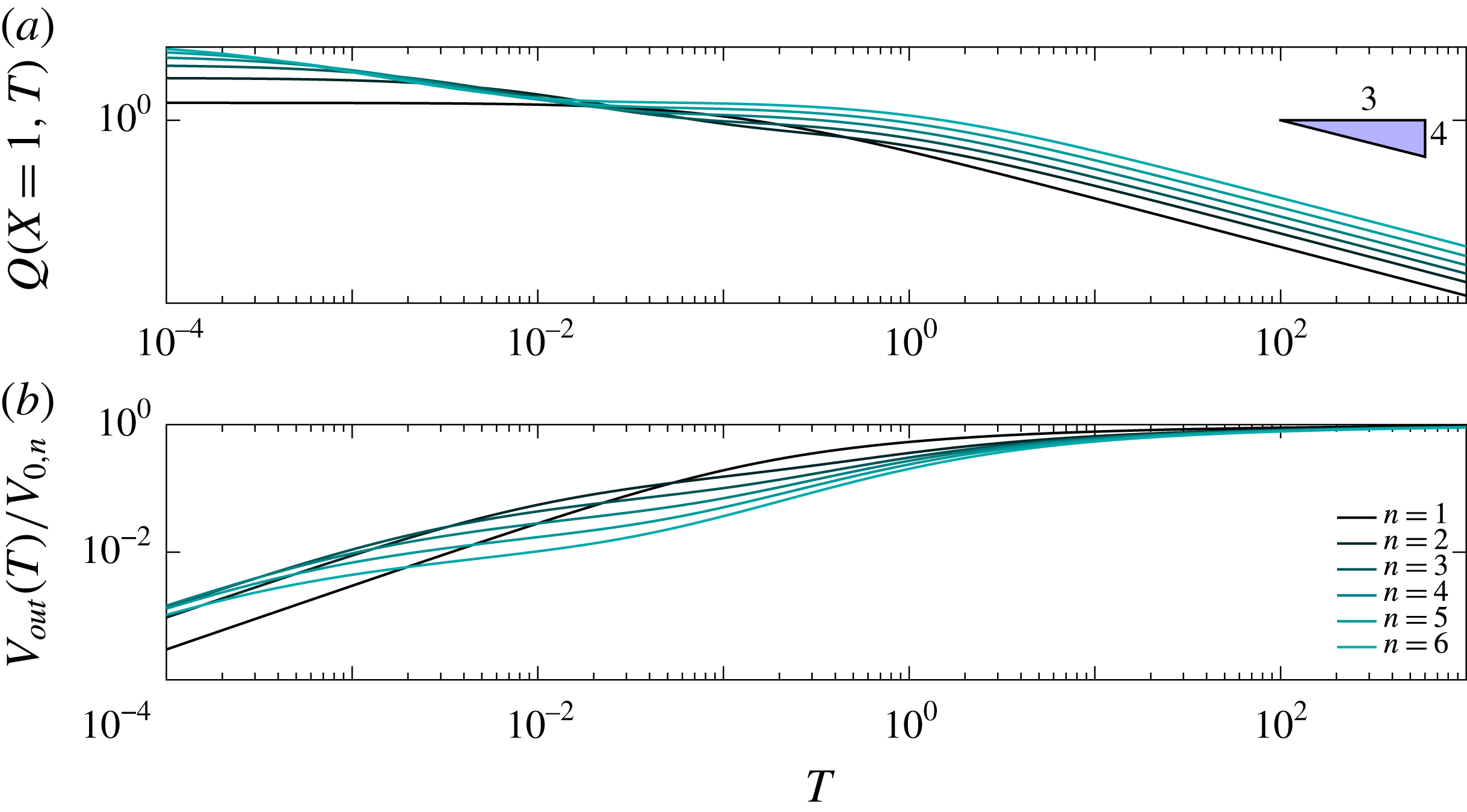
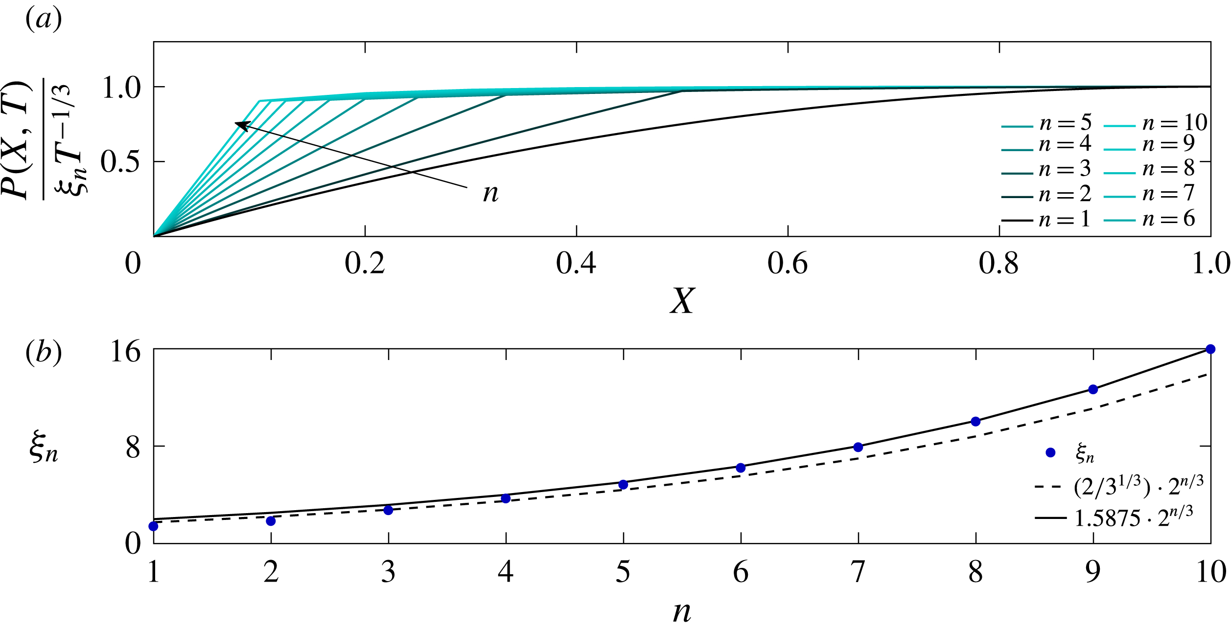
Equations (4.5) are now to be solved numerically subject to (4.6). We also comment that the
 $T^{-1/3}$
asymptotic behaviour holds for this model network system. The systematic changes as
 $n$
increases are shown in figures 8 and 9. In figure 8 we again introduce the pre-factor
 $\unicode[STIX]{x1D709}_{n}$
as the coefficient in
 $P_{n-1}(1,T)\sim \unicode[STIX]{x1D709}_{n}T^{-1/3}$
for any given network size
 $n$
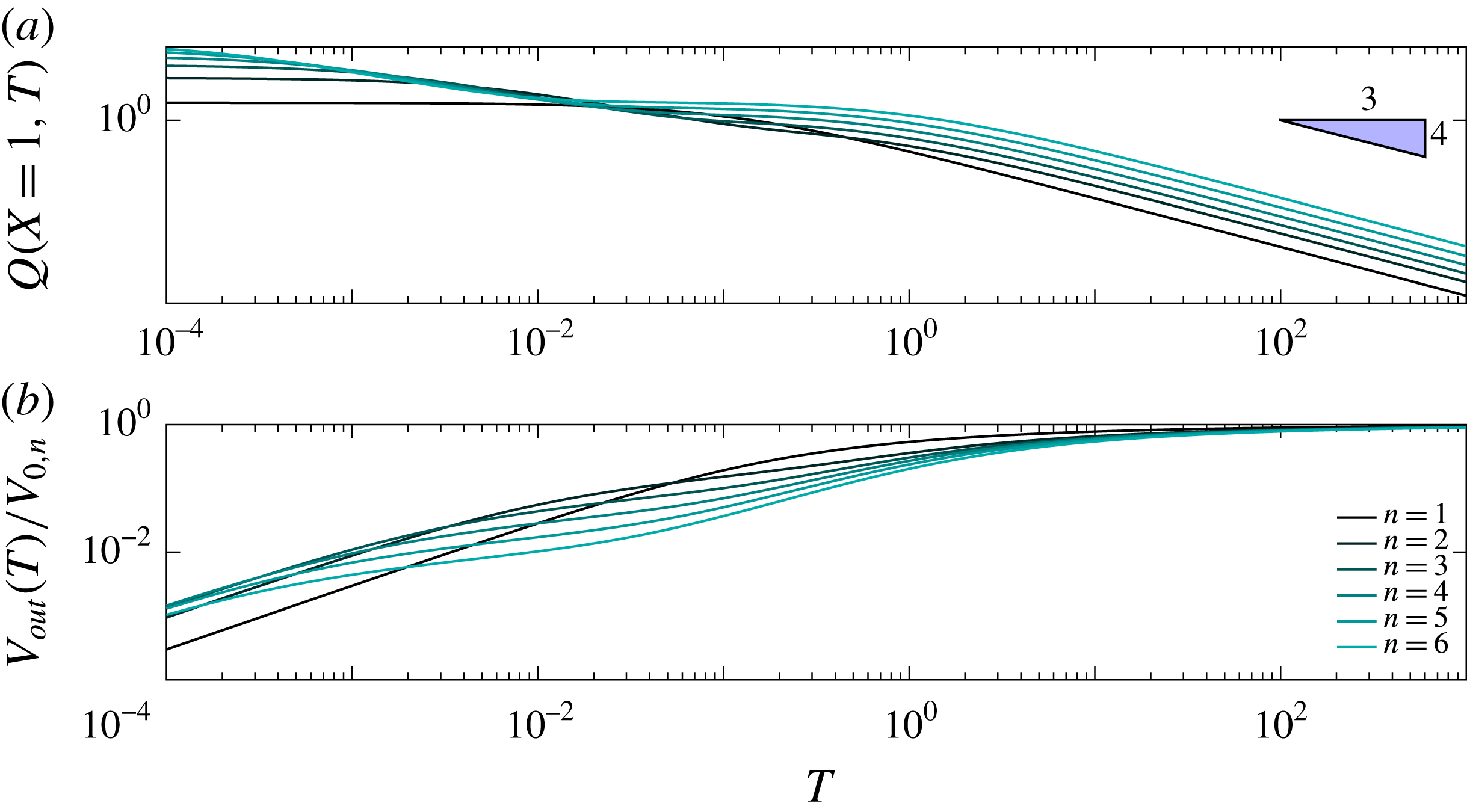
. Figure 9(a) shows the dimensionless network outlet flow rate
 $Q$
and figure 9(b) shows the cumulative volume of rejected fluid
 $V_{out}(T)$
normalized by initial volume of retained fluid in the network
 $V_{0,n}$
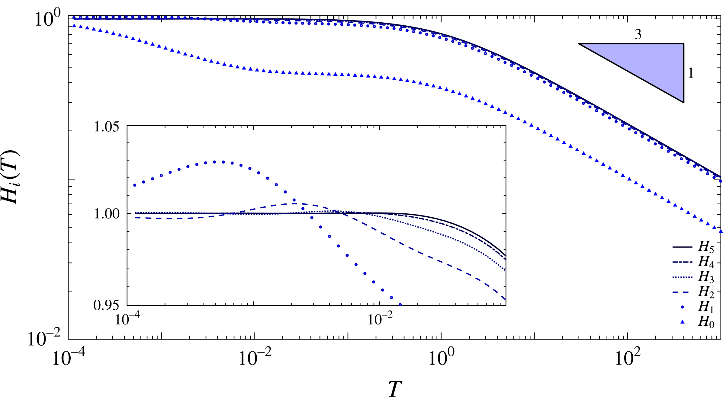
. Aperture size evolution in time across different fracture generations for a system of
 $n=6$
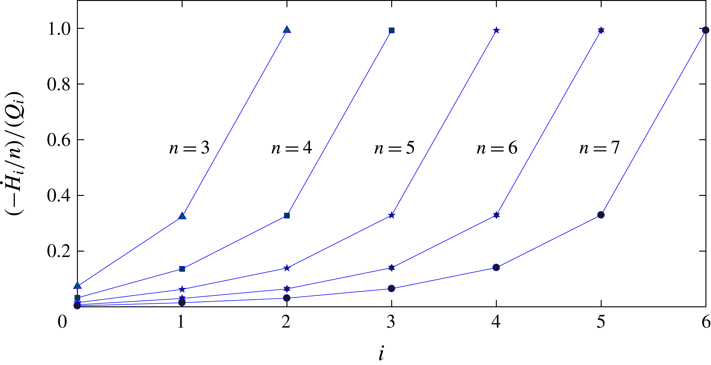
is shown in figure 10. We also investigate the driving force for the flow at every generation in figure 11 by presenting the ratio between the flux
 $-{\dot{H}}_{i}/n$
generated by squeezing of a channel in the
 $i$
th generation and the total outlet flux
 $Q_{i}=-\sum _{k=i}^{n-1}2^{k-i}{\dot{H}}_{k}/n$
of that channel. The innermost fracture is always unity as the no-flux boundary condition, equation (4.6e
), prevents any inward flow at all times (figure 11). It is evident for
 $n>3$
that the next generation has only
 ${\sim}30\,\%$
of its total flux driven by the squeezing force. The following generations exhibit even lesser fractions due to the increased volume flux along the flow path.
Aperture size distributions in time between generations for
 $n=6$
.

Late-time ratio between the flux driven by the squeezing force and the total outlet flux at every generation for various values of
 $n$
. The flux ratio for the innermost fracture,
 $H_{n-1}$
, is always unity since it never has any inward flux as defined by (4.6e
).

4.3 Asymptotic solution for late times and large
$n$

The pressure in the network of branched channels is approximately uniform away from the outlet at late times (figure 8
a), indicating that the backflow is mainly limited by the outermost channel. In the rest of the system, the fluid flows relatively freely since the channels are held open by a larger pressure and also due to the larger volume represented by multiple parallel channels. This physical insight allows us to develop an asymptotic description of the system, valid for
 $T\gg 1$
and
 $n\gg 1$
. As before, a scaling analysis reveals that
 $H_{i}$
and
 $P_{i}$
can be expected to behave like
 $T^{-1/3}$
as
 $T\rightarrow \infty$
.
First, we consider the region away from the outlet, in which the pressure is approximately uniform. We thus assume that
 $P_{i}\sim \unicode[STIX]{x1D709}_{n}T^{-1/3}$
, and the force balance (4.5b
) yields the approximate fracture apertures
 $$\begin{eqnarray}\displaystyle H_{i}\sim \frac{\unicode[STIX]{x1D709}_{n}}{n}T^{-1/3}. & & \displaystyle\end{eqnarray}$$
Multiplying the fracture aperture by a single fracture length we get the two-dimensional fracture volume, and then multiplying by the approximate number of fractures in the system we obtain a leading-order approximation for the entire network volume,
 $$\begin{eqnarray}\displaystyle V_{tot}\sim \frac{2^{n}\unicode[STIX]{x1D709}_{n}}{n^{2}}T^{-1/3}. & & \displaystyle\end{eqnarray}$$
The time rate of change of the system volume yields the total flux leaving the network,
 $$\begin{eqnarray}\displaystyle Q_{0}\sim \frac{1}{3}\frac{2^{n}\unicode[STIX]{x1D709}_{n}}{n^{2}}T^{-4/3}. & & \displaystyle\end{eqnarray}$$
Now we consider the outlet channel with unknown aperture
 $H_{0}$
which controls the outflow. Using (2.2) we can approximate the pressure gradient to leading order as
 $Q_{0}/H_{0}^{3}$
. Integrating this we obtain an approximate pressure profile
 $$\begin{eqnarray}\displaystyle P_{0}(X,T)\sim \frac{Q_{0}}{H_{0}^{3}}X. & & \displaystyle\end{eqnarray}$$
In order to find
 $H_{0}$
, we substitute this into the force balance (4.5b
) where
 $i=0$
. The resulting equation for
 $H_{0}$
can be solved to yield
 $$\begin{eqnarray}\displaystyle H_{0}\sim \left(\frac{Q_{0}}{2n^{2}}\right)^{1/4}. & & \displaystyle\end{eqnarray}$$
Substituting (4.11) back into (4.10), and then equating the pressure
 $P_{0}(1/n,T)$
at the inlet of the first fracture to the constant pressure
 $\unicode[STIX]{x1D709}_{n}T^{-1/3}$
in the bulk of the network yields the approximation
 $$\begin{eqnarray}\displaystyle \unicode[STIX]{x1D709}_{n}\approx \frac{2}{3^{1/3}}2^{n/3}. & & \displaystyle\end{eqnarray}$$
As we can see from figure 8, this gives the correct behaviour
 $\unicode[STIX]{x1D709}_{n}\propto 2^{n/3}$
but the numerical pre-factor is different. This is because the pressure drops in the other channels near the outlet are small but not asymptotically negligible, and our result must be adjusted by including these.
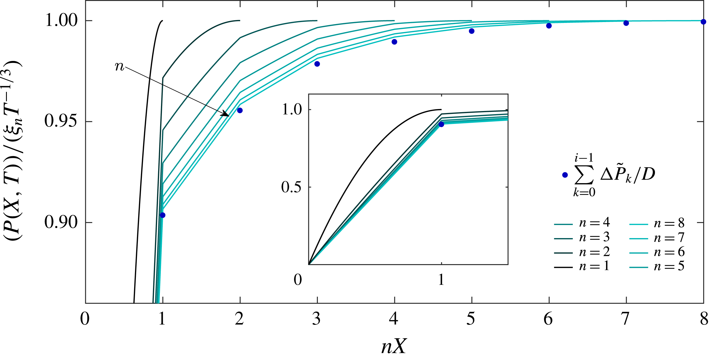
Late-time pressure profiles rescaled by their maximum value and stretched from the outlet to make each channel length unity. The inset presents the range of values not captured in the main plot to allow for better resolution of the inner channels.

In order to consider the other channels, we now let
 $\tilde{H}_{i}T^{-1/3}$
and
 $\unicode[STIX]{x0394}\tilde{P}_{i}T^{-1/3}$
be the aperture and pressure drop across the
 $i$
th generation of channels, respectively, and
 $Q_{0}=\tilde{Q}_{0}T^{-4/3}$
is the flux from the outlet channel. Assuming
 $Q_{0}$
is the leading-order flux through all channels, the pressure profile in each channel is approximately linear with pressure gradient
 $$\begin{eqnarray}\displaystyle \frac{\unicode[STIX]{x0394}\tilde{P}_{i}T^{-1/3}}{1/n}=\frac{\tilde{Q}_{0}T^{-4/3}}{2^{i}(\tilde{H}_{i}T^{-1/3})^{3}}, & & \displaystyle\end{eqnarray}$$
which yields an expression for
 $\tilde{H}_{i}$
in terms of
 $\unicode[STIX]{x0394}\tilde{P}_{i}$
,
 $$\begin{eqnarray}\displaystyle \tilde{H}_{i}=\left(\frac{\tilde{Q}_{0}}{n2^{i}\unicode[STIX]{x0394}\tilde{P}_{i}}\right)^{1/3}. & & \displaystyle\end{eqnarray}$$
The average pressure in the
 $i$
th fracture is
 $$\begin{eqnarray}\displaystyle \unicode[STIX]{x0394}\tilde{P}_{0}T^{-1/3}+\unicode[STIX]{x0394}\tilde{P}_{1}T^{-1/3}+\cdots +\unicode[STIX]{x0394}\tilde{P}_{i-1}T^{-1/3}+{\textstyle \frac{1}{2}}\unicode[STIX]{x0394}\tilde{P}_{i}T^{-1/3}. & & \displaystyle\end{eqnarray}$$
Multiplying the average pressure by the fracture length again yields the integrated pressure in the fracture which according to (4.5b ) provides the following algebraic system:
 $$\begin{eqnarray}\displaystyle \mathop{\sum }_{k=0}^{i-1}\unicode[STIX]{x0394}\tilde{P}_{k}+\frac{1}{2}\unicode[STIX]{x0394}\tilde{P}_{i}=nH_{i}=\left(\frac{n^{2}\tilde{Q}_{0}}{2^{i}\unicode[STIX]{x0394}\tilde{P}_{i}}\right)^{1/3}. & & \displaystyle\end{eqnarray}$$
Solving for
 $\unicode[STIX]{x0394}\tilde{P}_{i}$
iteratively using Mathematica yields the total pressure drop
 $$\begin{eqnarray}\displaystyle \mathop{\sum }_{k=0}^{\infty }\unicode[STIX]{x0394}P_{k}T^{-1/3}=D(n^{2}\tilde{Q}_{0})^{1/4}T^{-1/3},\quad D\approx 1.86128, & & \displaystyle\end{eqnarray}$$
where the upper limit of the sum can be taken to infinity since
 $n$
is large and the series converges rapidly. The result for
 $D$
is, as expected, larger than the approximation,
 $D\approx 2^{3/4}\approx 1.6818$
, obtained above from considering the outlet channel only. Equating this pressure drop with the bulk pressure
 $\unicode[STIX]{x1D709}_{n}T^{-1/3}$
and using
 $\tilde{Q}_{0}=2^{n}\unicode[STIX]{x1D709}_{n}/(3n^{2})$
, (4.9), then yields
 $$\begin{eqnarray}\displaystyle \unicode[STIX]{x1D709}_{n}\sim \frac{D^{4/3}}{3^{1/3}}2^{n/3}\approx 1.5875\times 2^{n/3}. & & \displaystyle\end{eqnarray}$$
This result is in excellent agreement with the numerical results in figure 8. As for the pressure profiles, figure 12 shows the rescaled profiles taken from figure 8(a) with the horizontal axis stretched to make all channels the same length for the different values of
 $n$
and the outlets aligned. As
 $n$
increases, it is clear that the profiles tend towards a universal shape, namely a piecewise linear profile with the pressure drop across each channel given by the asymptotic predictions (4.16).
We conclude that our asymptotic solution has accurately captured the physical processes governing the backflow, and can be used to predict the late-time behaviour of the system without having to resort to costly numerical calculations.
5 Discussion
Motivated by the environmental concerns from hydraulic fracturing operations, we studied backflow dynamics after the injection pressure was released, and the fracturing liquids flow back. As a preview to the ensuing discussion, it is useful to estimate the magnitudes of possible time scales, mainly to reflect on the importance and relevance of early- and late-time behaviours. Since no two shales are alike, and fracturing fluid composition varies throughout the industry, we present a range of possible values (Clarkson & Williams-Kovacs Reference Clarkson and Williams-Kovacs2013; Sone & Zoback Reference Sone and Zoback2013). For example,
 $\unicode[STIX]{x1D707}\sim 10^{-3}{-}10^{-1}$
Pa s,
 $E\sim 10{-}100$
GPa,
 $h^{\ast }/L=\unicode[STIX]{x1D716}\sim 10^{-4}{-}10^{-2}$
, where the lower limit describes a less viscous fluid (water) in a more rigid medium with a larger aspect ratio, and the upper limit a more viscous fluid in a less rigid medium with a smaller aspect ratio. Since the time scale still depends on the unknown magnitude of
 $\hat{E}$
(through unknown property
 $l_{0}$
which signifies the initial thickness of the elastic foundation and may be related to the spacing between fractures), it is important to establish its magnitude in order to evaluate the time scale. It is further noted that the model assumption of a quasi-stationary process may become invalid at times smaller than the viscous scale,
 ${h^{\ast }}^{2}/\unicode[STIX]{x1D708}$
, where
 $\unicode[STIX]{x1D708}$
is the fluid’s kinematic viscosity. With an aperture range of
 $h^{\ast }\sim 10^{-3}{-}10^{-1}$
m we estimate the viscous time to be
 ${h^{\ast }}^{2}/\unicode[STIX]{x1D708}\sim 10^{-2}{-}10^{4}$
s. For the smallest system,
 $n=2$
,
 $l_{0}$
must be of the order of
 $10^{5}$
m, which is non-physical, while in the upper limit
 $l_{0}$
should be in the range of
 $10^{-4}{-}10^{2}$
meaning that early times are only relevant around the upper limit in small systems. For
 $n=100$
, the lower limit shows that
 $l_{0}\in [1,10^{6}]$
m is sufficient to justify the consideration of early times, while the upper limit requires that
 $l_{0}\leqslant 10^{-3}$
m which seems unlikely.
Another possibly important effect not considered in the current model is fracture roughness, which can limit the minimum aperture size and modify the flow rate. Brown (Reference Brown1987), Thompson & Brown (Reference Thompson and Brown1991) postulated that when a fracture is formed, the two surfaces are juxtaposed at a specified separation defined in terms of the mean surface separation, which, in this paper can be regarded as
 $H(T)$
and the standard deviation of the local aperture,
 $\unicode[STIX]{x1D70E}_{H}$
, according to
 $H(T)/\unicode[STIX]{x1D70E}_{H}$
. Their results showed that when the surfaces are widely separated (i.e.
 $H(T)\gg \unicode[STIX]{x1D70E}_{H}$
), roughness has very little effect, but at the limit where
 $H(T)/\unicode[STIX]{x1D70E}_{H}\sim 1$
, fluid is expected to take a tortuous path and thus deviations from the cubic law (i.e.
 $Q\propto -H^{3}\unicode[STIX]{x1D735}P$
) are expected. However, the effect of roughness can be approximated through the incorporation of an ‘effective’ aperture (Zimmerman, Kumar & Bodvarsson Reference Zimmerman, Kumar and Bodvarsson1991) allowing the flow rate to exactly satisfy the cubic law. The present model is valid while
 $h^{\ast }\gg \unicode[STIX]{x1D70E}_{H}$
, i.e.
 $H(T)\gg \unicode[STIX]{x1D70E}_{H}/h^{\ast }$
. Given the late-time asymptotic behaviour
 $H(T)\sim T^{-1/3}$
, we can thus expect the validity to extend until the very late time
 $T_{r}\sim (h^{\ast }/\unicode[STIX]{x1D70E}_{H})^{3}$
, where
 $T_{r}$
is the time scale for the roughness to become of consequential magnitude.
5.1 Effect of network size
In the previous sections, formulations and solutions for an elastic response to a pre-strained condition in a network of bifurcating fractures have been presented. All models have been shown to admit a late-time asymptotic behaviour towards a
 $T^{-1/3}$
time dependence, in good agreement with experimental results reported by Lai et al. (Reference Lai, Zheng, Dressaire, Ramon, Huppert and Stone2016a
). Pressure distributions have been shown to collapse at late times to a single universal curve when scaled using their time dependence, and approximate solutions were derived for large
 $n$
. Examining the systematic changes in pressure distribution, as shown in figure 8, it is evident that rise in complexity of the fracture network (i.e. increase in
 $n$
) decreases the effective region of the pressure gradient driving fluids from the network to the wellbore, to a radius equivalent in size to the length of the outermost fracture, denoted by subscript
 $0$
. In the presented case, the above mentioned effective region decreases by an order of magnitude to a mere 10 % of the length of the entire network with
 $n=8$
. However, we note that for a case of decreasing fracture lengths with generation propagation, the effective region should be substantially greater. Flow rates tend at late times to a
 $T^{-4/3}$
dependence and exhibit higher values with increasing
 $n$
as presented in figure 9(a). However, figure 9(b) shows that the rejected volume fraction relative to the initially retained volume is smaller with increasing
 $n$
, thus larger networks (i.e. larger
 $n$
) are less effective in evicting fluids. Ghanbari & Dehghanpour (Reference Ghanbari and Dehghanpour2016) suggested that the retained fluid in more complex networks may imbibe in place of retained hydrocarbons and so increase hydrocarbon production in the backflow period. Our asymptotic analysis shows that the backflow process is controlled by the channels near the outlet where the total cross-section for the flow is smaller, and the bulk of the network acts as a reservoir. Asymptotic analysis for large
 $n$
has shown that for fixed outlet properties, there is a finite value
 $n$
above which all networks will behave similarly, as the pressure jump within each inner fracture decays towards zero (figure 12). This is also evident by the differences in squeezing force effect between generations at large
 $n$
as seen in figure 11.
5.2 Late-time aperture size distribution
Another interesting observation that can be made from figures 5 and 10 is that at late times, for every network size,
 $H_{i}<H_{i+1}$
, so that flow is transmitted from thicker to thinner cracks. This is apparent from the elasticity equation since the pressure decreases downstream, as seen in figure 8. The total volume contained at every couple of transmitting channels is twice larger than the volume of the receiving channel. The increased volume flux at every further node is met with a decreased total cross-section for the flow. This leads to the somewhat surprising consequence that the flux is larger through narrower channels. However, this is not a contradiction, but merely means that the pressure drop must be larger near the root, which is indeed what we see in figure 12. This observation is especially interesting here since the simple geometry of our model essentially captures some upper cutoff case for the volume flux. Taking into consideration any decay in the scale of fracture dimensions upstream from the outlet, the transmitting channels should probably provide lower flow rates as a result of a smaller volume of the transmitting channel or of the total volume of the preceding network allowing the pressure gradient to better distribute along the network.
Pressure losses around the junctions due to bends and abrupt changes in cross-sectional area for the flow may be important to include in some cases. However, in two dimensions, in a three-way junction between three channels with aperture
 $O(h)$
, we expect the junction to also have aperture
 $O(h)$
, and so the pressure gradient inside the junction is comparable to the pressure gradient in the channels. Since the junction is short compared with the length of each channel, the net pressure drop across the junction can be neglected. This would not be true for the case where two randomly oriented cracks in three dimensions with a similar aspect ratio touch at a point, forming a connection with a very small cross-section relative to the cross-section of either crack, but since our network is formed by bifurcation from a single starting point, this issue would not apply.
The analysis performed in this paper lays the foundation for the study of fracture networks. However, late-time behaviour in the real world, would probably show some effects that were not considered in this paper. Two such major effects would probably be fracture roughness and permeability. The former becomes important to the flow, when the aperture size approaches the magnitude of the roughness. Namely, at the limit where
 $H/\unicode[STIX]{x1D70E}_{H}\sim 1$
or
 $T\sim (h^{\ast }/\unicode[STIX]{x1D70E}_{H})^{3}$
. The latter holds great importance especially when applying the model to real processes in shale.
This work provides insights for predicting the backflow dynamics in practical hydraulic fracturing operations, and can be useful, for example, informing engineering design or the design of legal and regulatory frameworks for the backflow of the fracturing liquids.
Acknowledgements
A.D. acknowledges the support from the Nancy and Stephen Grand Technion Energy Program (GTEP) and the Israeli Ministry of National Infrastructures, Energy and Water Resources under the student scholarship program for degrees in the field of energy. The research was also supported, in part, by a grant from the Royal Society International Exchange Fund.
Appendix A. Network numerical simulations
The numerical results for the network problem in § 3 were obtained using Matlab subroutine ‘ODE15s’; the time span was set to the range
 $[0,1000]$
. Relative and absolute tolerances were set to
 $10^{-5}$
. The PDEs (partial differential equations) were reduced to ODEs using Mathematica, with the equations solved being
 $$\begin{eqnarray}\displaystyle & \displaystyle \frac{\text{d}H_{0}(T)}{\text{d}T}=\frac{48H_{0}^{3}(T)[H_{0}^{4}(T)+6H_{0}(T)H_{1}^{3}(T)-3H_{1}^{4}(T)]}{2H_{0}^{3}(T)+3H_{1}^{3}(T)}, & \displaystyle\end{eqnarray}$$
 $$\begin{eqnarray}\displaystyle & \displaystyle \frac{\text{d}H_{1}(T)}{\text{d}T}=\frac{24H_{0}^{3}(T)H_{1}^{3}(T)[3H_{0}(T)-2H_{1}(T)]}{2H_{0}(T)^{3}+3H_{1}(T)^{3}}, & \displaystyle\end{eqnarray}$$
 $$\begin{eqnarray}\displaystyle & \displaystyle a_{1}(T)=-\frac{\dot{H_{0}}+2\dot{H_{1}}}{2\dot{H_{0}}}, & \displaystyle\end{eqnarray}$$
 $$\begin{eqnarray}\displaystyle & \displaystyle a_{2}(T)=0, & \displaystyle\end{eqnarray}$$
 $$\begin{eqnarray}\displaystyle & \displaystyle b_{1}(T)=-1, & \displaystyle\end{eqnarray}$$
 $$\begin{eqnarray}\displaystyle & \displaystyle b_{2}(T)=-\frac{H_{1}^{3}\dot{H_{0}}-3H_{0}^{3}\dot{H_{1}}+4H_{1}^{3}\dot{H_{1}}}{8H_{0}^{3}\dot{H_{1}}}, & \displaystyle\end{eqnarray}$$