
1. Introduction
The flow around a pair of circular cylinders has been considered as a canonical problem for studying the effects of flow interference. Extensive reviews are given in Sumner (Reference Sumner2010) and Zhou & Mahbub Alam (Reference Zhou and Mahbub Alam2016). For identical cylinders of diameter  $D$ placed in a side-by-side arrangement with distance
 $P$ between their centres, the following regimes of interference can be singled out (Zdravkovich Reference Zdravkovich1987):
(i) A single vortex street at
 $D\leqslant P < P_1$ ($P_1/D=1.1\text {--}1.2$), when the flow behind a pair of cylinders resembles the flow past a single bluff body.
(ii) A biased gap flow (bistable) at
$P_1 < P < P_2$ ($P_2/D=2\text {--}2.2$), when narrow and wide wakes are formed, which are the consequence of the jet forming in the gap and biased towards the narrow wake. Such a flow is bistable and can intermittently change sides with narrow and wide wakes.(iii) Coupled vortex streets at
$P_2 < P < P_3$ ($P_3/D=4\text {--}5$), when two vortex streets are developed as a result of synchronised vortex shedding.


There are quite a few studies on how these regimes of interference affect aerodynamic forces, the Strouhal number and wake patterns (see the reviews mentioned above); however, not so much research has been carried out on heat transfer. Such data for an incompressible viscous fluid flow around side-by-side cylinders with an isothermal boundary condition can be found in Zhou, Zhang & Yiu (Reference Zhou, Zhang and Yiu2002), Hu & Zhou (Reference Hu and Zhou2008), Yoon, Seo & Kim (Reference Yoon, Seo and Kim2010) and Chaitanya & Dhiman (Reference Chaitanya and Dhiman2012), but the knowledge on compressible viscous fluid flow behind side-by-side cylinders is not sufficient. For a single cylinder, the compressibility effect at low Reynolds numbers has been recently studied numerically and experimentally by Canuto & Taira (Reference Canuto and Taira2015), Gu et al. (Reference Gu, Barber, John and Emerson2019) and Nagata et al. (Reference Nagata, Noguchi, Kusama, Nonomura, Komuro, Ando and Asai2020a).
The present work studies the total enthalpy redistribution in a compressible viscous fluid flow behind side-by-side thermally insulated cylinders at Reynolds numbers  $Re\leqslant 10^3$ (defined by diameter
 $D$), free-stream Mach numbers
 ${M_{\infty }}\leqslant 0.8$ and different interference regimes. Specifically, the effect of a significant decrease in the recovery temperature of the rear part of a thermally insulated cylinder – the Eckert–Weise effect (Eckert & Weise Reference Eckert and Weise1942) – and redistribution of the total enthalpy (total temperature) in the wake are under consideration. Apart from the fundamental interest, the results of the research can be useful regarding the field of low-Reynolds-number compressible aerodynamics, e.g. the flight of small aircraft in an exotic environment such as the atmosphere of Mars – this problem has attracted attention due to the possibility of a Martian terrain survey (Munday et al. Reference Munday, Taira, Suwa, Numata and Asai2015).
Another field of application is machine-free energy separation devices, such as the Ranque–Hilsch tube (Eiamsa-ard & Promvonge Reference Eiamsa-ard and Promvonge2008) and the Leontiev tube (Leont'ev Reference Leont'ev1997; Leontiev et al. Reference Leontiev, Zditovets, Vinogradov, Strongin and Kiselev2017), which convert a gas flow into two output flows with significantly different stagnation temperatures without external heat supply and work. Ways of increasing the effectiveness of the Leontiev tube is the subject of much current research (Azanov & Osiptsov Reference Azanov and Osiptsov2017; Kiselev et al. Reference Kiselev, Leontiev, Vinogradov, Zditovets and Strongin2019; Leontiev et al. Reference Leontiev, Zditovets, Kiselev, Vinogradov and Strongin2019). This energy separation device is based on heat exchange between gas flows having significantly different velocities (sub- and supersonic) and identical stagnation parameters; they are separated by a thin wall with low thermal resistance. The key idea is that the recovery temperature for a sub- and supersonic flow differs considerably for a heat-insulated wall. That is why heat exchange between the flows occurs in the case of a heat-conducting separation wall, resulting in a change of stagnation temperature in the flow. Thus, the intensification of energy separation is related to an increase in heat exchange. In particular, Kiselev et al. (Reference Kiselev, Leontiev, Vinogradov, Zditovets and Strongin2019) showed that the introduction of a transverse circular cylinder increases the heat transfer coefficients of the wall (compared to a case without a cylinder) due to the interaction of the cylinder wake and the boundary layer of the wall. The energy separation in the wakes has a value for turbine flows as well, since the non-uniform distribution of the stagnation temperature behind the stator blade row can create specific incoming thermal conditions for the rotor (see the review by Sieverding & Manna Reference Sieverding and Manna2020).
In this regard, the understanding of energy separation processes in canonical problems such as a flow around cylinders with the effects of interference is of substantial importance. It allows one to model various interactions of the forming vortices with the rear part of the body surface and the structures of the formed wakes, which determines the intensity of the Eckert–Weise effect (Aleksyuk & Osiptsov Reference Aleksyuk and Osiptsov2018) and correspondingly the degree to which the total enthalpy can be lowered in the central part of the wake (Kurosaka et al. Reference Kurosaka, Gertz, Graham, Goodman, Sundaram, Riner, Kuroda and Hankey1987; Aleksyuk Reference Aleksyuk2019).
For an isolated cylinder, the problem of energy separation has been discussed in many, mostly experimental, studies (Ryan Reference Ryan1951; Thomann Reference Thomann1959; Eckert Reference Eckert1987; Kurosaka et al. Reference Kurosaka, Gertz, Graham, Goodman, Sundaram, Riner, Kuroda and Hankey1987; Ng, Chakroun & Kurosaka Reference Ng, Chakroun and Kurosaka1990; Goldstein & Kulkarni Reference Goldstein and Kulkarni2008; Kulkarni & Goldstein Reference Kulkarni and Goldstein2009; Aleksyuk & Osiptsov Reference Aleksyuk and Osiptsov2018; Burazer Reference Burazer2018). The distribution of time-averaged total enthalpy  $\overline {i_0}$ has considerably reduced values at the base of the cylinder and near the wake centreline, which weaken downstream (Thomann Reference Thomann1959; Goldstein & Kulkarni Reference Goldstein and Kulkarni2008). A detailed qualitative view of the total enthalpy distributions can be obtained using numerical simulations (Kurosaka et al. Reference Kurosaka, Gertz, Graham, Goodman, Sundaram, Riner, Kuroda and Hankey1987; Aleksyuk & Osiptsov Reference Aleksyuk and Osiptsov2018). The most pronounced reduction of total enthalpy
 $i_0$ is observed near the rear part of the body and is associated with vortex formation, since the change of the total enthalpy along the boundary layer (at the front part of the cylinder) does not provide an observed level of
 $i_0$ reduction. As suggested by Ryan (Reference Ryan1951), the connection of the Eckert–Weise effect with the vortex shedding process was also implicitly confirmed by Kurosaka et al. (Reference Kurosaka, Gertz, Graham, Goodman, Sundaram, Riner, Kuroda and Hankey1987): it was shown that a considerable decrease in
 $i_0$ can be obtained by the intensification of vortices using the resonance between the frequencies of standing acoustic waves in the wind tunnel and the vortex shedding process.
The Mach-number influence on the Eckert–Weise effect was discussed by Zdravkovich (Reference Zdravkovich1997, pp. 515–517) based on a compilation of measurements of the recovery factor  $r_T=(T-T_\infty )/(T_0-T_\infty )$ at the rear point of the cylinder (Eckert Reference Eckert1984), further denoted by
 $r_{TB}$, where
 $T$ is the fluid temperature, and subscripts ‘
 $0$’ and ‘
 $\infty$’ denote stagnation and incoming flow parameters. Following the classification of flow regimes with respect to the Mach number given in Zdravkovich (Reference Zdravkovich1997, p. 500):
 $r_{TB}$ increases in the small-Mach-number (‘shockless’) regime at
 ${M_{\infty }}\lesssim 0.4$; decreases in the intermittent shock regime
 $0.4\lesssim {M_{\infty }}\lesssim 0.65$, when weak shock waves alternate on both sides of the cylinder; and, again, increases in the regimes of permanent shocks at
 $0.65\lesssim {M_{\infty }}\lesssim 0.8$ and near-wake shocks at
 $0.8\lesssim {M_{\infty }}\lesssim 1$. The latter two regimes correspond to the appearance of permanent shocks that, with an increase of
 ${M_{\infty }}$, are moving downstream, elongating and displacing the vortex formation region by delaying the position of the shear layer rollup (this effect will also be seen in the presented numerical simulations in § 4). This is consistent with the close connection of the formation process with the intensity of the Eckert–Weise effect. There is also a strong dependence of the intensity of the effect on the Reynolds number, since it highly influences the vortex formation process (Williamson Reference Williamson1996; Zdravkovich Reference Zdravkovich1997).
The energy separation can be explained by considering conservation of  $i_0$ in fluid particles (Eckert Reference Eckert1987; Kurosaka et al. Reference Kurosaka, Gertz, Graham, Goodman, Sundaram, Riner, Kuroda and Hankey1987). From the energy conservation law
 \begin{equation} \frac{\textrm{D} i_0}{\textrm{D}t} =\underbrace{\frac{1}{\rho}\frac{\partial p}{\partial t}}_{\mathcal{P}} + \underbrace{\frac{1}{\rho Re}\boldsymbol{\nabla}\boldsymbol{\cdot} (\boldsymbol{\tau}\boldsymbol{\cdot}{\boldsymbol{u}})}_{\mathcal{A}} +\underbrace{\frac{\gamma}{\rho RePr}\nabla^2 T}_{\mathcal{Q}}, \end{equation}
in a laminar flow (see § 2.1 for definitions of variables), the redistribution of total enthalpy  $i_0$ in fluid particles can be caused by: the time variation of pressure (
 $\mathcal {P}$); the work of viscous stresses (
 $\mathcal {A}$); and the heat conduction (
 $\mathcal {Q}$). Assuming that the non-stationarity and dissipative mechanisms are insignificant (as in the flow outside the wake), one can obtain that the total enthalpy is conserved, i.e.
 $i_0=i_{0\infty }=\text {const.}$, where
 $i_{0\infty }$ is the free-stream total enthalpy. In fact, in the developed wake, it is reasonable to assume that only the first term defines the process of energy separation. Based on this, Kurosaka et al. (Reference Kurosaka, Gertz, Graham, Goodman, Sundaram, Riner, Kuroda and Hankey1987) suggested a simple explanation of gas cooling near the wake centreline taking into account that in front of the vortices
 $\partial p/\partial t<0$ and the particles are moving towards the wake, having a decreasing
 $i_0$ (and vice versa for the particles behind the vortices). By tracking the trajectories of fluid particles in Aleksyuk & Osiptsov (Reference Aleksyuk and Osiptsov2018), this was fully supported numerically based on the Navier–Stokes equations.
Using the point vortex model for the classical Kármán vortex street model (with Rankine vortices instead of the potential ones), Kurosaka et al. (Reference Kurosaka, Gertz, Graham, Goodman, Sundaram, Riner, Kuroda and Hankey1987) gave the relation between the total enthalpy and the parameters of the vortex street (period of street  $l$, vortex circulation
 $\varGamma _0$ and its velocity
 $1+U$ in the reference frame fixed to the cylinder) as
 \begin{equation} \overline{i_0}-i_{0\infty}={-}\frac{\varGamma_0}{l}(1+U), \end{equation}
where time-averaged values are denoted by overbars. Aleksyuk (Reference Aleksyuk2019) considered a similar model in the general case of wake structures consisting of  $N$ vortex chains and demonstrated quite good agreement of the obtained estimates with the numerical results considering local regions of a two-dimensional wake behind a transversely oscillating circular cylinder. Thus, having a specific structure of the wake, one can estimate total enthalpy redistribution based on simple point vortex models. Less clear is the situation when the large-scale structures in the wake are disordered: some new considerations in this regard are presented in § 4. Even for disordered wakes, the transverse profiles of
 $\overline {i_0}$ are closely related to the profiles of velocity.
Such simple models do not work well in the formation region due to the tangled trajectories of fluid particles (see Aleksyuk & Osiptsov Reference Aleksyuk and Osiptsov2018) and a potential need to take into account all the mechanisms (because, a priori, it is not obvious which of the mechanisms plays the defining role). Moreover, for a model case of  $Re=10^3$,
 ${M_{\infty }}=0.4$ and
 $Pr=0.72$, it was shown that all of them are of the same order near the rear part of the cylinder. That is why further clarification of the Eckert–Weise effect is still needed through careful consideration of the development of the recirculation zones near the surface of the body. The key elements of this process are singled out in § 5, and it turns out that the Eckert–Weise effect is mainly caused by the influence of the
 $\mathcal {P}$ mechanism and entrainment towards the surface of heated and cooled gas portions by forming vortices.
The present article uses numerical simulations in the framework of a two-dimensional flow of a viscous perfect gas at two Reynolds numbers  $Re=200$ and
 $10^3$, Mach numbers
 ${M_{\infty }}=0.1$,
 $0.4$ and
 $0.8$, and with Prandtl number fixed to
 $Pr=0.72$; the problem formulation is given in § 2. This model allows one to grasp the key underlying physics (see § 3) and to get details on the mechanisms responsible for the redistribution of energy in the flow (§§ 4 and 5). Numerical results are discussed in two parts: the first part (§ 4) is devoted to the general influence of the flow parameters on the patterns of energy separation in the developed wake and its efficiency; the second one (§ 5) is the discussion of the action of mechanisms responsible for energy separation near the body surface. Each section is divided into two subsections where we separately discuss the general mechanisms responsible for particular energy separation phenomena (usually by considering simplified models or the flow behind a single cylinder) and the influence of flow interference behind side-by-side cylinders.
2. Problem formulation and numerical method
2.1. Problem formulation
The problem is formulated in the Cartesian coordinate system  $(x, y)$ chosen so that the centres of the cylinders have coordinates
 $(0, 0)$ and
 $(0, P)$ and the incoming flow has the velocity
 $(u_\infty , 0)$; see figure 1. The cylinders are assumed to have diameters
 $D$. The cylinder placed at
 $x=y=0$ will be called the first or the lower one, and the other cylinder is the upper or the second one.
Side-by-side arrangement of two circular cylinders in a cross-flow.

The fluid flow is described by a model of a viscous perfect gas with constant specific heats  $c_V$ and
 $c_p$ at constant volume and pressure, and thermal conductivity
 $\kappa$ and viscosity
 $\mu$ coefficients. The compressible fluid motion is governed by the Navier–Stokes equations in the non-dimensional form:
 \begin{gather} \frac{\textrm{D} \rho}{\textrm{D} t}+\rho\boldsymbol{\nabla}\boldsymbol{\cdot}\boldsymbol{u}=0, \end{gather}
 \begin{gather}\rho\frac{\textrm{D} \boldsymbol{u}}{\textrm{D} t}={-}\boldsymbol{\nabla} p + \frac{1}{Re}\boldsymbol{\nabla} \boldsymbol{\cdot}\boldsymbol{\tau}, \end{gather}
 \begin{gather}\rho\frac{\textrm{D}}{\textrm{D}t}\left(T+\frac{1}{2}\boldsymbol{u}^2\right) ={-}\boldsymbol{\nabla} \boldsymbol{\cdot}(p\boldsymbol{u}) +\frac{1}{Re}\boldsymbol{\nabla}\boldsymbol{\cdot} (\boldsymbol{\tau}\boldsymbol{\cdot}\boldsymbol{u} ) +\frac{\gamma}{RePr}\nabla^2 T, \end{gather}
where the matrix of viscous stress tensor  $\boldsymbol {\tau }$ components is
 \begin{equation} (\tau_{ij})=\begin{pmatrix} \displaystyle\frac{4}{3}\frac{\partial u}{\partial x}-\frac{2}{3}\frac{\partial v}{\partial y} & \displaystyle\frac{\partial u}{\partial y}+\frac{\partial v}{\partial x} \\ \displaystyle\frac{\partial u}{\partial y}+\frac{\partial v}{\partial x} & \displaystyle\frac{4}{3}\frac{\partial v}{\partial y}-\frac{2}{3}\frac{\partial u}{\partial x} \end{pmatrix}. \end{equation}
These equations are further considered in primitive variables, which are pressure  $p$, velocity
 $\boldsymbol {u}$ and temperature
 $T$ (using the equation of state
 $\rho =(\gamma -1)^{-1}p/T$). The solution is parametrised by the Reynolds number
 $Re=\rho _\infty u_\infty D/\mu$, the Prandtl number
 $Pr=\mu c_p/\kappa$, the Mach number
 ${M_{\infty }}=u_\infty /c_\infty$ and the distance between the cylinders
 $P/D$, where
 $\rho _\infty$ is the free-stream density,
 $c_\infty =\sqrt {{\gamma p_\infty }/ {\rho _\infty }}$ is the sonic velocity in the free stream and
 $\gamma =1.4$ is the specific heat ratio. The non-dimensionalisation is performed using the relations
 \begin{equation} t=\frac{u_\infty t'}{D},\quad \boldsymbol{x}=\frac{\boldsymbol{x}'}{D},\quad p=\frac{p'}{\rho_\infty u_\infty^2},\quad \boldsymbol{u}=\frac{\boldsymbol{u}'}{u_\infty},\quad T=\frac{c_V T'}{u_\infty^2}, \end{equation}
in which dimensional quantities are denoted by primes.
The following boundary conditions are assumed. On the cylinder surface, the velocity no-slip  $\boldsymbol {u}=(0,0)$ and adiabatic-wall
 $\boldsymbol {\nabla } T\boldsymbol {\cdot }\boldsymbol {n}=0$ conditions are prescribed (where
 $\boldsymbol {n}$ is the unit normal vector). At infinity,
 $\boldsymbol {u}=(1,0)$,
 $p={1/{(\gamma\;{M_{\infty }}^2)}}$ and
 $T={1/{[\gamma (\gamma -1)\;{M_{\infty }}^2]}}$.
2.2. Numerical method and influence of computational parameters
Initial-boundary value problems are numerically solved by the Galerkin least-squares finite-element method on unstructured triangular meshes with the implicit Euler method for the time derivative. The resulting system of nonlinear algebraic equations is solved by a combination of the Newton iterative and the generalised minimal residual methods. More details on the numerical algorithm and examples of its application can be found in Aleksyuk & Osiptsov (Reference Aleksyuk and Osiptsov2018) and Aleksyuk & Shkadov (Reference Aleksyuk and Shkadov2018). To reduce the influence of artificial far boundaries on the region of interest (the boundary layers and the near wake at  $-1 < x < 20$), the domain size is chosen to be
 $[-200, 400]\times [-200, 200]$.
For the convergence test, the bistable shedding regime at  $P/D=1.5$ is considered since it corresponds to a disordered wake structure. Further, the case at
 $Re=10^3$,
 ${M_{\infty }}=0.4$ and
 $Pr=0.72$ is discussed.
Figure 2 shows aerodynamic coefficients and normalised distribution of  $\overline {i_0}$ for three time steps
 $\Delta t=0.00125$,
 $0.0025$ and
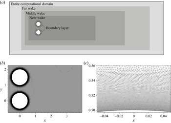
 $0.005$ and meshes M-1 and M-2. Mesh M-1 has a nested structure (figure 3) with the following resolutions in the regions of interest: in the near wake (
 $-1.5\leqslant x\leqslant 26$) and near the surface of the cylinders the step size is approximately
 $0.025$ and
 $0.0005$ respectively (the resolution in other subregions is shown in table 1). These correspond to approximately 40–70 computational nodes across the formed vortices, as well as the dynamic and thermal boundary layers at
 $Re=10^3$ and
 $Pr=0.72$. Mesh M-2 has a two-fold finer spatial resolution. The time-averaging procedure and spectral analysis are carried out over the interval
 $100\leqslant t\leqslant 1100$ with time resolution
 $0.01$ for forces and
 $0.2$ for variables distribution.
Influence of temporal ( $\Delta t$) and spatial (mesh M-1 has twice the cell size than mesh M-2) resolution on the coefficients of drag
 $C_D(t)$ (a) and lift
 $C_L(t)$ (b), and on the time-averaged distribution of
 $\overline {I_0}$ (c) at
 $Re=10^3$ and
 ${M_{\infty }}=0.4$. Aerodynamic coefficients in panels (a) and (b) for the upper and lower cylinders are shown in red and black, respectively; lines of the same type in panel (c) show contour levels
 $\overline {I_0}=-0.005, -0.015,\ldots , -0.055$ and various line types correspond to different resolutions (see notation to right of the plot).

Computational mesh: (a) schematic representation of nested subregions with different sizes of triangular elements (table 1), denoted by ‘Boundary layer’, ‘Near wake’, ‘Middle wake’ and ‘Far wake’; (b,c) fragments of the mesh M-1 used for calculations at  $P/D=1.5$ in the near wake and close to the wall.

Parameters of the main meshes. Here,  $\varDelta$ is the approximate size of triangular elements of the mesh;
 $X_{in}$ and
 $X_{out}$ are the distances from the
 $y$-axis to the inlet and outlet of the corresponding subdomain; and
 $H$ is its height. The mesh size near the walls smoothly changes in annular regions from
 $\varDelta =0.0005$ (
 $0.002$) at the circle
 $r=0.5$ (
 $r=0.55$) to
 $\varDelta =0.002$ (
 $0.025$) at
 $r=0.55$ (
 $r=0.7$), where
 $r=\sqrt {x^2+y^2}$.

The dependences of drag  $C_D(t)$ and lift
 $C_L(t)$ coefficients on time in figure 2(a,b) show a disordered character of the flow. Nevertheless, from the spectral analysis the main frequency (i.e. Strouhal number
 $St$, which is defined by
 $D$ and
 $u_\infty$) is clearly identified to be equal to
 $St=0.2445\pm 0.004$ for all the considered time and space resolutions (the average over both cylinders’ frequencies is used, which were obtained from the lift coefficients). The aerodynamic coefficients (i.e.
 $0.5(\overline {C_{D1}}+\overline {C_{D2}})=1.5172$ and
 $0.5(|\overline {C_{L1}}|+|\overline {C_{L2}}|)=0.3572$) at
 $\Delta t=0.0025$ and M-1 differ by less than
 $4\,\%$ from the results with the other time steps and mesh M-2.
Time-averaged distributions of total enthalpy are used as an indicator of energy transitions in the flow. In particular, the minimal values of  $\overline {I_0}$ on the surface of the cylinders, in the formation region (
 $x<3$) and in the developed wake (
 $3\leqslant x\leqslant 20$) are assessed. That is why it is worth comparing the influence of the computational parameters on such distributions. In figure 2(c) we use normalised total enthalpy
 $I_0$ defined by the expression
 \begin{equation} I_0=\frac{i_0-i_{0\infty}}{i_{0\infty}}, \quad i_0=\gamma T_0=\gamma T+0.5 (u^2+v^2 ). \end{equation}
Normalisation allows assessment of the percentage of  $i_{0}$ change in fluid particles due to the presence of the obstacles. Additionally,
 $I_0$ is equal to normalised total temperature
 $(T_0-T_{0\infty })/T_{0\infty }$, where
 $T_0$ is the total temperature and subscript ‘
 $\infty$’ denotes free-stream parameters. That is why the regions with decreased (increased) values of
 $I_0$ are further also called cooled (heated) fluid regions. The total enthalpy is constant along streamlines in a stationary flow in the absence of dissipative mechanisms (see (1.1)); hence,
 $I_0\approx 0$ far from the body and the wake. One can see an acceptable match of
 $\overline {I_0}$ distributions in figure 2(c). More precisely, the local minimum of
 $\overline {I_0}$ is
 $-0.0536$ at
 $\Delta t=0.0025$ and mesh M-1; this value differs by less than
 $3.2\,\%$ from the calculations at the other considered computational parameters.
Thus, despite the flow bistability and irregularity, the influence of computational parameters is not considerable taking into account the fact that we are aiming at a qualitative description of physical processes. In this article,  $\Delta t=0.0025$ and mesh M-1 are used.
3. Consistency of numerical simulation results
The results of the present work are mainly based on a model that does not take into account some of the real flow physics such as three-dimensionality and small-scale turbulent fluctuations. That is why it would be unjustifiable to expect a quantitative agreement with the experimental data. Indeed, as soon as the flow becomes three-dimensional at  $Re\approx 180$ (Williamson Reference Williamson1988; Barkley & Henderson Reference Barkley and Henderson1996) due to the instability of flow structures developing in the formation region (see e.g. Aleksyuk & Shkadov Reference Aleksyuk and Shkadov2018), the aerodynamic coefficients start to diverge from two-dimensional simulations: for example, at
 $Re=10^3$ the experimental time-averaged drag coefficient
 $\overline {C_D}$ is approximately 1.5 times smaller than that taken from two-dimensional simulations for the incompressible flow conditions (Roshko Reference Roshko1961; Henderson Reference Henderson1995). Nevertheless, the two-dimensional model can reproduce key flow features, such as shear layer instability and the drag crisis at high Reynolds numbers, since the key mechanisms responsible for these phenomena are related to the development of the large-scale structures (Singh & Mittal Reference Singh and Mittal2005; Dynnikova Reference Dynnikova2008). Similarly, one may expect that the model can grasp the main physical processes responsible for the total enthalpy redistribution. The two-dimensional model reproduces key flow features such as the time-averaged distribution of total enthalpy in the developed wake and the Eckert–Weise effect (Aleksyuk & Osiptsov Reference Aleksyuk and Osiptsov2018).
The details of these phenomena can differ. Figure 4 shows a comparison of the calculated surface distribution of recovery factors
 \begin{equation} r_T=\frac{T-T_\infty}{T_0-T_\infty}\quad\text{and}\quad r_p=\frac{p-p_\infty}{p_0-p_\infty} \end{equation}
at  $Re=10^3$ and
 ${M_{\infty }}=0.4$ with the data of pioneering experiments on energy separation at higher Reynolds numbers
 $Re\approx 10^5$ and Mach numbers
 ${M_{\infty }}\approx 0.4$ (Eckert & Weise Reference Eckert and Weise1942; Ryan Reference Ryan1951), as well as the experimental pressure distribution by Nagata et al. (Reference Nagata, Noguchi, Kusama, Nonomura, Komuro, Ando and Asai2020a) at
 $Re=4\times 10^3$ and two-dimensional numerical simulations by Singh & Mittal (Reference Singh and Mittal2005) for an incompressible flow at
 $Re=2\times 10^2$,
 $2\times 10^3$,
 $10^4$ and
 $10^5$. One can clearly observe the manifestation of the Eckert–Weise effect in two-dimensional simulations (regions with
 $\overline {r_T}<0$ in figure 4a) and qualitative similarities in
 $\overline {r_p}$ curves (figure 4b). Despite that, quantitative differences in
 $\overline {r_T}$ are observed starting from
 $\theta \approx 60\text {--}80^\circ$, when the pressure gradient changes its sign. At the front part of a cylinder the behaviour of the curves is quite similar. This suggests a considerable dependence of the temperature distribution of the rear part of the cylinder on the particular way in which vortices are developed in the formation region, which is sensitive to the Reynolds number for both real and model flows.
Qualitative agreement of the experimental and model surface distribution of recovery factors  $\overline {r_T}$ (a) and
 $\overline {r_p}$ (b): the solid red line represents the present calculation; the symbols are the experimental data by Eckert & Weise (Reference Eckert and Weise1942) (
 $\square$), Ryan (Reference Ryan1951) (
 ${\scriptstyle {\bigcirc} }$) and Nagata et al. (Reference Nagata, Noguchi, Kusama, Nonomura, Komuro, Ando and Asai2020a) (
 $\triangle$); the dashed blue lines correspond to simulations by Singh & Mittal (Reference Singh and Mittal2005) (an incompressible fluid model). Isentropic theory relations were used to convert
 $T/T_0$ and
 $p/p_0$ from Ryan (Reference Ryan1951) and pressure coefficient
 $C_p$ from Nagata et al. (Reference Nagata, Noguchi, Kusama, Nonomura, Komuro, Ando and Asai2020a) into
 $r_T$ and
 $r_p$ given by (3.1a,b).

The latter can be seen in the  $\overline {C_p}$ distribution of Singh & Mittal (Reference Singh and Mittal2005) shown in figure 4(b): first, the time-averaged base suction coefficient
 $-C_{p_B}$ (where
 $C_{p_B}=\overline {C_p}|_{\theta =180^\circ }$) is growing with the increase of
 $Re$ and then begins to decay at
 $Re\approx 10^4$ as the small-scale vortices resulting from the shear layer instability approach the cylinder and narrow the width of the wake. A similar process takes place in a real flow at higher Reynolds numbers (starting at approximately
 $Re\approx 1.2\times 10^5$). It should be noted that
 $r_p$ tends to
 $C_p$ in the incompressible limit, since
 $p'_0-p'_\infty \rightarrow 0.5\rho _\infty u_\infty ^2$ (in dimensional variables).
The regimes of vortex formation processes in the incompressible limit can be well described by the base suction coefficient dependence on  $Re$ (Roshko Reference Roshko1993; Williamson Reference Williamson1996), since
 $C_{p_B}$ is inversely dependent on the formation length in the considered regimes. The comparison of the model and the real
 $C_{p_B}(Re)$ curves (see Singh & Mittal Reference Singh and Mittal2005) shows that two-dimensional simulations ‘skip’ intervals of non-monotonic behaviour of
 $C_{p_B}(Re)$ (for
 $180\lesssim Re\lesssim 260$) related to the three-dimensional transition and the interval of the base suction decrease (for
 $260\lesssim Re\lesssim 10^3$) caused by a growing fine-scale three-dimensional disorder (Roshko Reference Roshko1993; Williamson Reference Williamson1996). Since all the experimental data presented in figure 4 are obtained at
 $Re >10^3$, the discrepancies are mainly due to the influence of these three-dimensional phenomena overlooked by the model. In the present work, it is assumed that omitting these effects is not an obstacle for a correct description of the key physical reasons for the total enthalpy redistribution, because the two-dimensional model includes the following:
(i) all three possible physical mechanisms that change the total enthalpy in a fluid particle along its trajectory, namely pressure fluctuations, heat conduction and work due to viscous stresses; and
(ii) the important features of the flow that influence the pattern of total enthalpy, namely the vortex formation process, vortex streets, regimes of wake interference and compressibility effects like the appearance of shock waves – these features exhibit similarities with the experimental data (shown above and in later sections).
However, one should note that, due to the variety of flow regimes of the considered canonical problem, there can be situations (e.g. a post-critical regime with turbulent boundary layers) where three-dimensionality and/or turbulence may be of great importance to describe the process of energy separation. Nevertheless, in such cases the presented two-dimensional results may also give some extra insight.
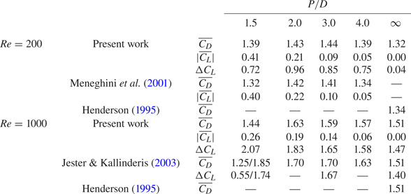
A quantitative comparison can be carried out with the two-dimensional numerical results of other authors. Thus, table 2 shows the comparison of aerodynamic coefficients with numerical simulations of a flow around side-by-side cylinders at  $Re=200$ (Meneghini et al. Reference Meneghini, Saltara, Siqueira and Ferrari2001) and
 $Re=10^3$ (Jester & Kallinderis Reference Jester and Kallinderis2003), as well as the results for a single cylinder at these Reynolds numbers (Henderson Reference Henderson1995). The incompressible flows are simulated by choosing a relatively small Mach number:
 ${M_{\infty }}=0.1$. For a single cylinder at
 $Re=10^3$, the presented data (
 $\overline {C_D}=1.511,\ St=0.2378$) differ from the reference data (Henderson Reference Henderson1995; Wen & Lin Reference Wen and Lin2001) (
 $\overline {C_D}=1.5092,\ St=0.2372$) by less than
 $0.3\,\%$. The highest divergence for side-by-side arrangements is observed with the results of Jester & Kallinderis (Reference Jester and Kallinderis2003) at
 $P/D=1.5$ and may be explained by a non-regular nature of this bistable regime (other differences are below
 $7\,\%$). The effect of compressibility is tested by comparing the present results (
 $\overline {C_D}=1.431$,
 $\Delta C_L=0.333$ and
 $St=0.1615$) at
 $Re=100$,
 ${M_{\infty }}=0.4$ and
 $Pr=0.72$ with the data of Canuto & Taira (Reference Canuto and Taira2015) (
 $\overline {C_D}=1.45$,
 $\Delta C_L=0.328$ and
 $St=0.162$): the difference is less than
 $2\,\%$.
Comparison of time-averaged aerodynamic coefficients at  $Re=200$ and
 $10^3$ and
 ${M_{\infty }}=0.1$ with the data of Meneghini et al. (Reference Meneghini, Saltara, Siqueira and Ferrari2001), Jester & Kallinderis (Reference Jester and Kallinderis2003) and Henderson (Reference Henderson1995) (an incompressible flow model was used). In the present work, coefficients are averaged over two cylinders:
 $\overline {C_D}=0.5(\overline {C_{D1}}+\overline {C_{D2}})$,
 $|\overline {C_L}|=0.5(|\overline {C_{L1}}|+|\overline {C_{L2}}|)$ and
 $\Delta C_L=0.5(\Delta C_{L1}+\Delta C_{L2})$, where
 $\Delta C_{L1}$ and
 $\Delta C_{L2}$ are the differences between maximum and average values. The averaged coefficients may differ considerably from the values over one of the cylinders in a biased regime due to flow asymmetry. Two values for both cylinders at
 $P/D=1.5$ and
 $Re=10^3$ are given in (Jester & Kallinderis Reference Jester and Kallinderis2003) and divided by the forward slash in the table; in other cases the data (Meneghini et al. Reference Meneghini, Saltara, Siqueira and Ferrari2001; Jester & Kallinderis Reference Jester and Kallinderis2003) are identical for both cylinders.

4. Energy transitions in the developed wake
The processes of energy separation in the developed wake and near the body are discussed separately in this and the next section, respectively. Such a possibility is justified by the independence of the corresponding physical reasons in the following sense. Figure 5(a) shows the energy separation scheme for the time-averaged flow in the near wake behind a single cylinder based on the calculation results shown in 5(b). In the instantaneous distributions of  $I_0$, heated and cooled portions of the fluid in the wake are clearly ordered so that the lowest values of
 $\overline {I_0}$ are observed near the centreline and the heated portions of the fluid have almost disappeared after averaging. The distribution of
 $\overline {i_0}$ can be described by its change along the time-averaged streamlines by the equation
 \begin{equation} \bar{\boldsymbol{u}}\boldsymbol{\cdot}\boldsymbol{\nabla} \overline{i_0} ={-}\overline{\boldsymbol{u}'\boldsymbol{\cdot}\boldsymbol{\nabla} i'_0} + \underbrace{\overline{\frac{1}{\rho} \frac{\partial p}{\partial t}}}_{\bar{\mathcal{P}}} + \underbrace{\frac{1}{ Re}\overline{\frac{1}{\rho} \boldsymbol{\nabla}\boldsymbol{\cdot} (\boldsymbol{\tau}\boldsymbol{\cdot}\boldsymbol{u})}}_{\bar{\mathcal{A}}} + \underbrace{\frac{\gamma}{RePr} \overline{\frac{1}{\rho}\nabla^2 T}}_{\bar{\mathcal{Q}}}, \end{equation}
where  $\boldsymbol {u}'=\boldsymbol {u}-\bar {\boldsymbol {u}}$ and
 $i'_0=i_0-\overline {i_0}$. The analysis by Aleksyuk & Osiptsov (Reference Aleksyuk and Osiptsov2018) of the terms on the right-hand side of (4.1) allows us to single out several regions that most significantly influence the change of
 $\overline {I_0}$ (the blue and red regions with a dashed border in 5a): in the thin boundary layer,
 $\overline {I_0}$ is decreasing; in the formation region, there is the most significant reduction of
 $\overline {I_0}$, which quickly recovers to some extent in the short red region; and in the stripes along the moving tails of shedding vortices,
 $\overline {I_0}$ is noticeably reducing, which forms a background of
 $\overline {I_0}<0$ in the developed wake. Owing to a change of vortex structure downstream, there can be other regions of
 $\overline {I_0}$ reduction, which will be discussed further. One should note that the flow in the boundary layer and the formation region is separated from the developed wake by bold streamlines in figure 5(a). This indicates that in a time-averaged sense there is no mutual influence on the energy separation process in these two regions.
Redistribution of total enthalpy in the flow behind a single cylinder. (a) Schematic division of a time-averaged flow into two parts (by bold streamlines) and the key cooling/heating subregions in the time-averaged flow. (b) Examples of calculated instantaneous and time-averaged distributions of  $I_0$ at
 $Re=10^3$ and
 ${M_{\infty }}=0.4$. The regions restricted by the dashed lines correspond to the most significant decay (blue colour) and growth (red colour) of
 $I_0$.

4.1. Simplified theoretical models
4.1.1. Point vortex model
In the developed vortex wake one can assume that the last two terms in (1.1) with small factors  $\textit {Re}^{-1}$ and
 $\gamma (\textit {Re}\textit {Pr})^{-1}$ are negligible. Hence, the evolution of
 $i_0$ can be approximately described by the simplified equation
 \begin{equation} \frac{\textrm{D} i_0}{\textrm{D}t}=\frac{1}{\rho}\frac{\partial p}{\partial t}. \end{equation}
This leads to a simple kinematic explanation of energy separation (Kurosaka et al. Reference Kurosaka, Gertz, Graham, Goodman, Sundaram, Riner, Kuroda and Hankey1987). For a classical Kármán vortex street, fluid particles move towards (away from) the wake centreline in front of (behind) the vortices, where  $\partial p/\partial t$ is negative (positive) because the pressure inside the vortices is less than that in the surrounding fluid. That is why the lowest values of
 $i_0$ are observed near the wake centreline (see figure 5).
The effect of the term  $\rho ^{-1}\partial p/\partial t$ in total enthalpy redistribution can be estimated by constructing a velocity field using reduced-order models, such as the point vortex model. The idea was applied in Kurosaka et al. (Reference Kurosaka, Gertz, Graham, Goodman, Sundaram, Riner, Kuroda and Hankey1987) for the classical staggered Kármán street and further generalised in Aleksyuk (Reference Aleksyuk2019) for arbitrary periodic vortex wakes, which are formed by
 $N$ infinite chains of vortices.
Under the assumptions that the flow is periodic in the  $x$-direction, inviscid, non-heat-conducting and the vortices are moving with constant velocity
 $1+U$ (
 $0<1+U<1$), one can obtain
 \begin{equation} \overline{i_0}(y)-i_{0\infty}={-} (1+U )[1-\bar{u}(y) ]. \end{equation}
The expression in square brackets can be further estimated by introducing the structure of the vortex wake. Let the vortices in each  $k$-chain have circulation
 $\varGamma _k$ (with
 $\varGamma _1+\varGamma _2+\cdots +\varGamma _N=0$),
 $y$-coordinate
 $y_k$, longitudinal period
 $l$ and radius
 $R_k$ of the vortex core (in the case when a Rankine vortex ‘patch’ is used to regularise a potential vortex). It is convenient to introduce parameters
 $\beta =lU/\varGamma <0$ and
 $\alpha _k=\varGamma _k/\varGamma$, which define the mutual arrangements of vortices (up to scaling of coordinates with
 $l$), with
 $\varGamma =|\varGamma _1|+|\varGamma _2|+\cdots +|\varGamma _N|$. The time-averaged component of velocity can be written in the form
 $\bar {u}(y)=1-(\varGamma /l)\,f(y, y_k, \alpha _k, R_k)$, where
 \begin{align} f(y, y_k, \alpha_k, R_k)&= \sum_{k=1}^{N}\frac{\alpha_k}{2}\textrm{sgn}(y-y_k)\nonumber\\ &\quad -\sum_{k=1}^{N}\frac{\alpha_k\theta_k(y)}{\rm \pi}\left[\textrm{sgn}(y-y_k) \arctan\sqrt{\left(\frac{R_k}{y-y_k}\right)^2-1}\right.\nonumber\\ &\quad -\left.\frac{y-y_k}{R_k}\sqrt{1-\left(\frac{y-y_k}{R_k}\right)^2}\,\right]. \end{align}
Here,  $\theta _k(y)$ equals one if
 $(y-y_k)^2 < R_k^2$; otherwise it is zero. The second sum on the right-hand side should be omitted if potential vortices without regularisation are used.
Thus, from (4.3) it follows that
 \begin{equation} \min_y\overline{i_0}(y)-i_{0\infty} ={-}\frac{\varGamma}{l}\left(1+\beta\frac{\varGamma}{l}\right) \max_y f(y, y_k, \alpha_k, R_k). \end{equation}
This means that the common belief that an increase in strength of vortices leads to the intensification of energy separation is ambiguous, since one should also take into account the change of spatial distribution of vortices. Indeed, for a given mutual arrangement of vortices ( $l$,
 $\beta$ and
 $\alpha _k$ are fixed), the optimal choice of
 $\varGamma$ is
 $\varGamma =-0.5l/\beta$, i.e.
 $\varGamma$ should be such that the velocity of vortices (
 $1+U$) is half of the free-stream value. Thus, at
 $\varGamma =-0.5l/\beta$, one has
 \begin{equation} \min_y\overline{i_0}(y)-i_{0\infty}=\frac{1}{4\beta}\max_y f(y, y_k, \alpha_k, R_k). \end{equation}
However, at fixed  $y_k$,
 $\alpha _k$ and
 $R_k$ (and
 $U=-0.5$), the arrangements of vortices with the lowest
 $|\beta |$ (i.e. highest
 $\varGamma /l$) correspond to the most intense energy separation. This ambiguity is related to the fact that the increase in
 $\varGamma$ with other parameters fixed can lead to the increase of the velocity defect
 $\max _y[1-\bar {u}(y)]$ simultaneously decreasing the velocity of vortices
 $1+U$. The described model allows estimation of the intensity of energy separation for specific wake patterns, as was shown in Aleksyuk (Reference Aleksyuk2019) by comparison with the numerical simulations assuming a weak dependence of the wake structure on
 $x$.
Interestingly enough, at a fixed  $x$, the similarity of profiles
 $\bar {u}(y)-1$ and
 $\overline {i_0}(y)-i_{0\infty }$ (see (4.3)) can still be observed even for disordered wakes. The example of distributions of
 $\overline {i_0}-i_{0\infty }$ and
 $k(\bar {u}-1)$ (
 $k=0.71$) at
 $\textit {Re}=10^3$,
 ${M_{\infty }}=0.4$ and
 $P/D=1.5$ is given in figure 6(a) and shows that they are very close. Figure 6(b,c) shows the possibility of finding coefficient
 $k<1$, such that curves
 $k(\bar {u}(y)-1)$ and
 $\overline {i_0}(y)-i_{0\infty }$ are very close to each other. This coefficient corresponds to the local velocity of vortices
 $(1+U)$ in (4.3).
Similarity of the distributions of time-averaged velocity component  $\bar {u}$ and total enthalpy
 $\overline {i_0}$: (a–c) the present calculation results for side-by-side arrangements of cylinders at
 $\textit {Re}=10^3$,
 ${M_{\infty }}=0.4$ and
 $P/D = 1.5$ (a,b) and 4 (c); and (d) the experimental data adopted from Goldstein & Kulkarni (Reference Goldstein and Kulkarni2008) for a single cylinder at
 $\textit {Re}=9.2\times 10^4$ and
 ${M_{\infty }}=0.22$ (
 $u_\infty$ was corrected to correspond to the velocity outside the wake). Black solid lines (black squares) and dashed red lines (red circles) correspond to the profiles of
 $\overline {i_0}-i_{0\infty }$ and
 $k(\bar {u}-1)$. In panel (a) contour levels are the same for
 $\overline {i_0}-i_{0\infty }$ and
 $k(\bar {u}-1)$ at
 $k=0.71$ (these levels are
 $-0.15, -0.25, \ldots , -0.85$).

Thus, the distribution of  $1-\bar {u}(x,y)$ gives an easy estimation of the energy separation pattern even for disordered wake structures. A similar comparison was conducted based on the experimental data of Goldstein & Kulkarni (Reference Goldstein and Kulkarni2008) in figure 6(d). It should be noted that, due to the restrictions of the test section in the spanwise direction (approximately
 $10.7D$ in total along the
 $y$-axis), the free-stream velocity outside the wake is considerably higher than the incoming flow velocity (
 $u_\infty$), hence, we used the approximation of the former as the reference value for non-dimensionalisation.
Based on the presented considerations, the recommendations to achieve high energy separation in the developed wake may be formulated as follows: the greater the velocity deficit and the longitudinal velocity of vortices, the lower values of  $\overline {I_0}$ can be achieved. Assuming that usually
 $1+U<1$, energy separation efficiency (
 $|\min \overline {I_0}|$) is always less than velocity deficit
 $1-\bar {u}(x,y)<1$ divided by
 $i_{0\infty }$. The latter gives an idea of the Mach-number dependence – it has the order of
 $i_{0\infty }^{-1}=(0.5+(\gamma -1)^{-1}\;{M_{\infty }}^{-2})^{-1}$.
4.1.2. Boundary layer approximation for the far wake
For the far wake, the estimation of total enthalpy distribution can be obtained using the boundary layer approximation in a way similar to that used to estimate the laminar velocity distribution (see Schlichting & Gersten Reference Schlichting and Gersten2017, p. 187). Assuming that in the laminar far wake the deviations  $u'$ and
 $T'$ of parameters
 $\bar {u}$ and
 $\bar {T}$ from the free-stream values are small, equations describing a compressible wake in the boundary layer approximation take the form:
 \begin{equation} \left.\begin{gathered} \frac{\partial u'}{\partial x}=\frac{1}{\textit{Re}}\frac{\partial^2 u'}{\partial y^2},\\ \frac{\partial T'}{\partial x}=\frac{1}{\gamma\textit{Re}\textit{Pr}}\frac{\partial^2 T'}{\partial y^2}. \end{gathered}\right\} \end{equation}
Using the following consequences of conservation laws at large enough values of  $x$,
 \begin{equation} \overline{C_D}=2\int\limits_{-\infty}^{\infty}\overline{\rho u(1-u)}\,{\textrm{d} y},\quad \int\limits_{-\infty}^{\infty}\overline{\rho u(i_0-i_{0\infty})}\,{\textrm{d} y}=0, \end{equation}
one can find a self-similar solution of equations (4.7). The resulting expressions for  $\bar {u}$ and
 $\overline {i_0}$ describing the asymptotic self-similar solution are as follows:
 \begin{gather} 1-\bar{u}=\sqrt{\frac{\textit{Re}}{{\rm \pi} x}}\,\frac{\overline{C_D}}{4}\exp{(-\textit{Re}\,y^2/4x)}, \end{gather}
 \begin{gather}i_{0\infty}-\overline{i_0}=(1-\bar{u})\left[1-\sqrt{\textit{Pr}}\exp{(-\textit{Re}(\textit{Pr}-1) y^2/4x)}\right]. \end{gather}
And since  $\overline {I_0}$ is proportional to
 $i_{0\infty }^{-1}$, then one obtains
 \begin{equation} \overline{I_0}={-}\;{M_{\infty}}^2\frac{(1-\bar{u})\left[1-\sqrt{\textit{Pr}}\exp{(-\textit{Re}(\textit{Pr}-1) y^2/4x)}\right]}{0.5\;{M_{\infty}}^2+1/(\gamma-1)}. \end{equation}
Relation (4.10) gives the following connection of the maximal values of total enthalpy and velocity deficits ( $\textit {Pr}\leqslant 1$):
 \begin{equation} \max_y(i_{0\infty}-\overline{i_0})= (1-\sqrt{\textit{Pr}} \,)\max_y(1-\bar{u}). \end{equation}
The proportionality coefficient does not depend on  $x$ and in our case gives rather a strong restriction, since
 $1-\sqrt {\textit {Pr}}\approx 0.15$. The highest efficiency of energy separation in the far wake is achieved in the limit
 $\textit {Pr}\rightarrow 0$. At
 $\textit {Pr}=1$ there is no energy separation in the asymptotic far wake due to the relation
 $i_{0\infty }-\overline {i_0}\approx \gamma (T_{\infty }-\bar {T})+1-\bar {u}$ and the balance between decrease in velocity (
 $\bar {u}<1$) and increase in the temperature (
 $\bar {T}>T_\infty$). It is worth noting that, in the central part of the near wake, temperature
 $T$ is lower (on average) than
 $T_\infty$, and gradually increases to the values greater than
 $T_\infty$; see figure 7. For the results shown in figure 7, mesh resolution in the wake was increased: the subregion called ‘Middle wake’ with approximate mesh resolution
 $\varDelta =0.06$ was extended in the
 $x$- and
 $y$-directions to
 $X_{out}=210$ and
 $H=25$, and the parameters of the ‘Far wake’ region were
 $X_{out}=260$ and
 $H=40$,
 $\varDelta =0.25$ (for notation, see figure 3 and table 1).
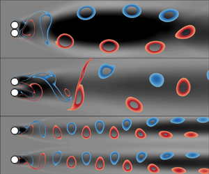
Distributions of vorticity (a) and normalised temperature  $(T-T_\infty )/T_\infty$ (b) behind an isolated cylinder at
 $\textit {Re}=10^3$ and
 ${M_{\infty }}=0.4$.

4.2. The influence of flow interference
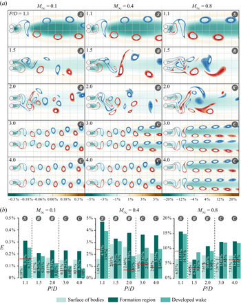
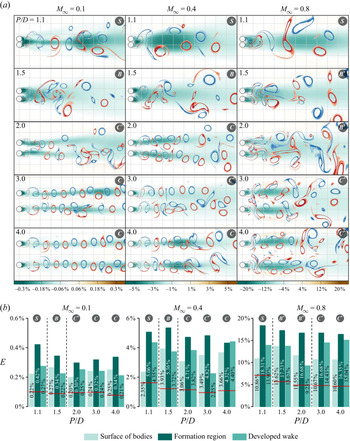
The influence of flow interference behind side-by-side cylinders is observed in figures 8(a) and 9(a), where the time-averaged total enthalpy  $\overline {I_0}$ distribution and instantaneous flow structure at various
 $P/D$ and
 ${M_{\infty }}$ at
 $\textit {Re}=200$ and
 $\textit {Re}=10^3$ are shown.
The influence of the distance between cylinders on the distribution of time-averaged total enthalpy at  $\textit {Re}=200$ and
 ${M_{\infty }}=0.1$, 0.4 and 0.8: (a)
 $\overline {I_0}$ and instantaneous wake patterns shown by the stripes of vorticity
 $0.7\leqslant |\omega |\leqslant 1.3$ (blue and red colours correspond to negative and positive values of
 $\omega$, respectively); and (b) efficiency of energy separation
 $E$ at the lower cylinder surface, the formation region and the developed wake (
 $E=|\min _{(x,y)} \overline {I_0}|$ is a local minimum); and integral efficiency
 $\hat {E}$ given by (4.13) and shown by horizontal red lines. Symbols in the grey circles denote the regime of interference: S, single vortex street; B, bistable vortex street;
 ${B}^*$, bistable vortex street, if the jet biased towards one of the wakes is not observed due to compressibility effects; and C, coupled vortex streets.

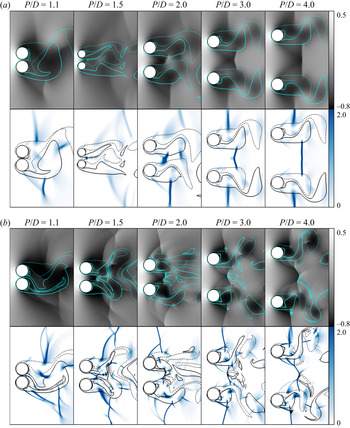
The influence of the distance between cylinders on the distribution of time-averaged total enthalpy at  $\textit {Re}=10^3$ and
 ${M_{\infty }}=0.1$, 0.4 and 0.8: (a)
 $\overline {I_0}$ and instantaneous wake patterns shown by the stripes of vorticity
 $0.5\leqslant |\omega |\leqslant 1.5$ (blue and red colours correspond to negative and positive values of
 $\omega$, respectively); (b) efficiency of energy separation
 $E$ at the lower cylinder surface, the formation region and the developed wake (
 $E=|\min _{(x,y)} \overline {I_0}|$ is a local minimum); and integral efficiency
 $\hat {E}$ given by (4.13) and shown by horizontal red lines. Symbols in the grey circles denote the regime of interference: S, single vortex street; B, bistable vortex street;
 ${B}^*$, bistable vortex street, if the jet biased towards one of the wakes is not observed due to compressibility effects; C, coupled vortex streets; and
 ${C}^*$, coupled vortex streets, in the absence of synchronisation or for a shifted one.

4.2.1. The instantaneous wake structure
The increase in  $\textit {Re}$ leads to more disordered wake patterns, a reduction of the formation length and an increase in the strength of the vortices, which are observed by comparing figures 8(a) and 9(a). In general, for both Reynolds numbers, the flow dependences on parameter
 $P/D$ are quite similar.
Three characteristic intervals of interference can be clearly seen for the considered Mach and Reynolds numbers: single (S), bistable (B) and coupled (C) vortex streets. There are several cases when two developed streets are clearly observed behind the cylinders at  $\textit {Re}=10^3$, but, nevertheless, the synchronisation of the vortex shedding process is absent (or shifted):
 ${M_{\infty }}=0.1,\ P/D=2.0$;
 ${M_{\infty }}=0.4,\ P/D=3.0$; and
 ${M_{\infty }}=0.8,\ P/D=3.0$ and
 $4.0$ (such regimes are denoted by symbol
 ${{C}}^*$ and for simplicity we continue to refer them to the coupled category). In addition, the effects of compressibility significantly change the flow in the gap between the cylinders at
 $\textit {Re}=10^3,\\;{M_{\infty }}=0.8,\ P/D=1.5$ and
 $2.0$, so the jet biased towards one of the wakes can no longer be observed (these situations are denoted by symbol
 ${{B}}^*$ and for simplicity we continue to refer them to the bistable category). The critical values of
 $P/D$ describing the boundaries between these regimes are influenced by
 ${M_{\infty }}$ and
 $\textit {Re}$. For both Reynolds numbers, the boundary between regimes S and B (
 ${{B}}^*$) is in the range
 $1.1\leqslant P_1/D \leqslant 1.5$; the second boundary between B (
 ${{B}}^*$) and C (
 ${{C}}^*$) lies in the ranges
 $2\leqslant P_2/D \leqslant 3$ at
 $\textit {Re}=200$ and
 $1.5\leqslant P_2/D \leqslant 2.0$ at
 $\textit {Re}=10^3$ (except for the case at
 ${M_{\infty }}=0.8$). These values are consistent with the experimental data for incompressible flows (small
 ${M_{\infty }}$) and the fact that
 $P_2(\textit {Re})$ is a decreasing function (see Zdravkovich Reference Zdravkovich1987; Xu, Zhou & So Reference Xu, Zhou and So2003).
When the Mach number equals  $0.8$, the transonic flow features become noticeable. The interaction of shock waves with the developed wake and their location at
 ${M_{\infty }}=0.8$ are demonstrated in figure 10. An increase in the Reynolds number leads to higher local Mach numbers and smaller thickness of shock waves, which is evidence of the reduction of the impact of viscous forces. A great diversity of interaction patterns is observed depending on
 $P/D$ and
 $\textit {Re}$, including the formation of
 $\lambda$-shaped and normal shocks on the sides, as well as in the space between the formation regions. Figure 10(b) shows that the intersection of shocks of opposite families in this space can result in the formation of curved shocks, leading to the generation of vorticity. In particular, this is the reason for a more complex wake structure and violation of synchronous vortex shedding, which is seen at
 $P/D=2$ and
 $3$ in figure 9(a).
Shock wave patterns at  ${M_{\infty }}=0.8$: normalised pressure distribution
 $(p-p_\infty )/p_\infty$ (in grey), positive pressure gradients along streamlines (in blue) and lines of constant vorticity (
 $\omega =\pm 1$) at
 $\textit {Re}=200$ (a) and
 $\textit {Re}=10^3$ (b). Regions of positive pressure gradients along streamlines are highlighted using the expression
 ${M}(\boldsymbol {u}/|\boldsymbol {u}|)\boldsymbol {\cdot }(\boldsymbol {\nabla }{p}/p)$, where
 ${M}$ is the local Mach number. Limit values on the colour maps are not maxima and minima of functions: function values greater than the upper limit (or less than the lower limit) are filled with one colour corresponding to this limit.

The significant effect of the Mach number seen from the figures is the increase of vortex formation length caused by the lateral shock waves on both sides of the formation region – this is most clearly observed at  $\textit {Re}=200$ and
 ${M_{\infty }}=0.8$ (figures 8a and 10a) and can be seen experimentally (Zdravkovich Reference Zdravkovich1997). A similar phenomenon is also observed in the flows behind axisymmetric bodies (Meliga, Sipp & Chomaz Reference Meliga, Sipp and Chomaz2010; Nagata et al. Reference Nagata, Nonomura, Takahashi, Mizuno and Fukuda2016, Reference Nagata, Nonomura, Takahashi and Fukuda2020b). This effect leads to the elongation of the corresponding subregion of reduced
 $\overline {I_0}$.
Oblique shock waves at the sides of the bodies (at  $|\theta |\lesssim 120^\circ$) are too weak to introduce noticeable changes in the total enthalpy redistribution on the surface. More generally, in the considered cases, compressibility effects (such as the interaction of shock waves with the forming vortices, a possible influence of shock waves on the boundary layer separation and the delays of the shear layer rollup) mainly influence the time-averaged total enthalpy distribution through the vortex formation process.
4.2.2. The time-averaged wake structure
In figures 8(a) and 9(a) the time-averaged total enthalpy patterns are clearly linked to the vortex wake structure. As well as for an isolated cylinder, in the single wake regime behind side-by-side cylinders ( $P/D=1.1$), there are two local regions with reduced
 $\overline {I_0}$: vortex formation and developed wake regions. As soon as vortices shed from both sides of each cylinder (at
 $P>P_1$), the cooled gas spot in the formation region is divided into two. The developed wake consists of one or two stripes of lowered
 $\overline {I_0}$ depending on whether the vortices shed from both cylinders are intensively interacting or not, respectively. For example, at
 $\textit {Re}=10^3$,
 ${M_{\infty }}=0.4$ and
 $P/D=2$ in figure 9(a), the synchronous vortex shedding regime produces two symmetric regions of reduced
 $\overline {I_0}$, which merge at
 $x>10$ due to the mixing of vortices from both vortex streets.
The intensity of energy separation is assessed by the local minima of  $\overline {I_0}$: the coefficient
 $E=|\min _{(x,y)\in \varOmega } \overline {I_0}(x,y)|$ is introduced in specific subregions
 $\varOmega$. The distributions of
 $\overline {I_0}$ in figures 8(a) and 9(a) show that it makes sense to consider the values of
 $E$ separately in the formation region and the developed wake. For the developed wake, the minimum is sought at
 $x<20$. Also, since the Eckert–Weise effect is of interest, the value of
 $E$ is considered at the surface of the cylinder (specifically, at the lower one). The three above-mentioned values of
 $E$ at various parameter values are given in figures 8(b) and 9(b). In these figures, the horizontal red lines show integral estimates for energy separation efficiency. The value is obtained by calculating the average of
 $|\overline {I_0}(x,y)|$ over the subdomain
 $\varOmega$, which corresponds to negative values of
 $\overline {I_0}(x,y)$ in the region of interest (
 $0 < x < 20$), i.e.
 $\varOmega =\{(x,y): \overline {I_0}(x,y) < 0\text { and }0 < x < 20\}$:
 \begin{equation} \hat{E}=\frac{\displaystyle\int_{\varOmega}|\overline{I_0}(x,y)|\,\textrm{d}x\,\textrm{d}y} {\displaystyle\int_{\varOmega}\,\textrm{d}x\,\textrm{d}y}. \end{equation}
The highest value of the integral estimate of intensity of energy separation  $\hat {E}$ is achieved at
 $P/D=1.1$, taking into account the area occupied by a considerably cooled fluid. On the contrary, on the surface of the cylinder,
 $E$ commonly has its lowest values at
 $P/D=1.1$ (this will be discussed in § 5). Here we concentrate on the flow in the wake. The difference between
 $E$ in the formation region and the developed wake varies depending on the flow regime. However, generally, the former region has a greater
 $E$ but a smaller area of considerably reduced
 $\overline {I_0}$.
Among the considered cases, only two regimes correspond to higher values of  $E$ in the developed wake:
 $\textit {Re}=200$,
 ${M_{\infty }}=0.8$,
 $P/D=1.5$ and
 $\textit {Re}=10^3$,
 ${M_{\infty }}=0.4$,
 $P/D=4$. Here, one should note that the connection of the energy separation intensity in the formation region (including the body surface) and in the developed wake is not straightforward. In the sense described at the beginning of this section, they can be considered independently. In the former case (
 $\textit {Re}=200$,
 ${M_{\infty }}=0.8$,
 $P/D=1.5$), lateral shock waves considerably change the process of vortex formation by moving the position of shear layer rollup downstream. That is why the impact of the pressure fluctuation mechanism on the energy redistribution in the formation region is reduced: the intensity becomes equal to
 $E|_{P/D=1.5}=6.22\,\%$ compared to
 $E|_{P/D=1.1}=15.55\,\%$ and
 $E|_{P/D=2.0}=10.68\,\%$. Consequently, the domination of
 $E$ in the developed wake is observed. Regarding the latter case (
 $\textit {Re}=10^3$,
 ${M_{\infty }}=0.4$,
 $P/D=4$), the effect is mainly due to the change of wake structure from a one-row to a double-row vortex street and can be explained by estimations using the point vortex model described in § 4.1.1 (similar examples are discussed by Aleksyuk (Reference Aleksyuk2019)). When the distance between the cylinders decreases to
 $P/D=3.0$, this wake reconstruction disappears and the intensity
 $E$ in the developed wake decreases by almost a factor of two (from
 $4.40\,\%$ to
 $2.25\,\%$). Besides, opposite changes occur in the formation region:
 $E$ increases from
 $4.32\,\%$ to
 $4.82\,\%$.
The increase in the Mach number considerably changes the efficiency  $E$; see figures 8(b) and 9(b). This is mostly related to the denominator
 $i_{0\infty }=0.5+(\gamma -1)^{-1}\;{M_{\infty }}^{-2}$ in the definition of
 $I_0$, which was pointed out in § 4.1 and can be observed from the calculation results. Assuming that
 $i_0-i_{0\infty }$ is of the same order for all Mach numbers, one can obtain that
 $E|_{\;{M_{\infty }}=0.4}\approx 15.5E|_{\;{M_{\infty }}=0.1}$ and
 $E|_{\;{M_{\infty }}=0.8}\approx 56.9E|_{\;{M_{\infty }}=0.1}$, which are comparable to the calculation results in figures 8(b) and 9(b).
By comparing figures 8(b) and 9(b) one can see that the increase in  $\textit {Re}$ leads to the growth in the energy separation efficiency for all the cases, which can be connected to the intensification of the vortex shedding process. For an isolated cylinder at
 ${M_{\infty }}=0.4$, the minimum of
 $\overline {I_0}$ changes from
 $-0.011$ to
 $-0.045$ in the interval
 $30\leqslant \textit {Re}\leqslant 500$ and only from
 $-0.045$ to
 $-0.048$ for
 $500\leqslant \textit {Re}\leqslant 1000$ (Aleksyuk & Osiptsov Reference Aleksyuk and Osiptsov2018).
5. Energy transitions in the formation region and the Eckert–Weise effect
As in the previous section, we first discuss the reasons for  $I_0$ redistribution behind a body and then the influence of flow interference on these processes.
5.1. Physical reasons for energy separation in the formation region
The dynamics of recirculation zones during the formation of vortices is responsible for specific distributions of  $I_0$ on the cylinder surface and the cooled fluid spot near the body, but the details of this process are not clear. The assessment of the time-averaged mechanisms in (4.1) allows us to single out regions and responsible mechanisms for
 $i_0$ growth and decay along time-averaged streamlines (figure 5). Within this framework, Aleksyuk & Osiptsov (Reference Aleksyuk and Osiptsov2018) showed that the sum
 $\bar {\mathcal {P}}+\bar {\mathcal {A}}+\bar {\mathcal {Q}}$ is small except for the boundary layer and a thin layer near the rear part of the cylinder. The defining role in the energy separation in the time-averaged sense belongs to the nonlinearity (
 $\overline {\boldsymbol {u}'\boldsymbol {\cdot }\boldsymbol {\nabla } i'_0}$), but the negative correlation
 $\overline {\boldsymbol {u}'\boldsymbol {\cdot }\boldsymbol {\nabla } i'_0}$ forms mainly due to the pressure fluctuations
 $\mathcal {P}$. In the present section, the link between the formation of vortices and the Eckert–Weise effect is constructed by singling out the key cooling and heating processes near the body surface. The periodic flow behind an isolated cylinder at
 $\textit {Re}=10^3$,
 ${M_{\infty }}=0.4$ and
 $\textit {Pr}=0.72$ is discussed as an example.
Figure 11 semi-schematically shows the evolution of  $I_0$ and
 $r_p$ in the formation region at approximately equidistant times
 $t_i$, such that
 $t_5-t_1$ is half of the vortex shedding period. Time
 $t_1$ corresponds to the initial stage of the vortex formation process, so that one can follow one vortex development. The spot of the cooled fluid (regions with reduced
 $I_0$) is growing and moving towards the wake centreline together with the forming vortex and losing its intensity as the vortex is shed in the wake. The vortex formation dynamics is also closely connected to the transformations of pressure distribution, thereby determining the action of mechanism
 $\mathcal {P}$ (see § 5.1.2).
Distributions of  $I_0$ and
 $r_p$ in the formation region behind an isolated cylinder at
 $\textit {Re}=10^3$ and
 ${M_{\infty }}=0.4$ and approximately equidistant times
 $t_i$, such that
 $t_5-t_1$ is half of the vortex shedding period. Dashed lines with arrows schematically represent the streamlines; the grey area inside the cylinder shows the pressure distribution over the surface; the black dots on the body surface are extrema of time-averaged functions
 $\overline {I_0}(\theta )$ (
 $I_0$ plots) and
 $\overline {r_p}(\theta )$ (
 $r_p$ plots); and the small insets show the instantaneous vorticity pattern in the near wake.

The corresponding time-averaged distribution of  $I_0$ in the wake and surface distributions of
 $r_T$ and
 $r_p$ are shown in figures 4 and 5. It should be noted that there is a simple connection between recovery factor
 $r_T$ and
 $I_0$:
 \begin{equation} r_T=1+2I_0i_{0\infty}. \end{equation}
One can see how the instantaneous distributions shown in figure 11 turn into the time-averaged ones (the extrema of  $\overline {I_0}$ and
 $\overline {r_p}$ are denoted by the black dots on the cylinder surface in figure 11). Hence, it is just necessary to explain the evolution of
 $I_0$ distributions in the near wake. Formally, this could be done by considering the change of
 $i_0$ in the fixed points of space using (4.1) in the following form:
 \begin{equation} \frac{\partial i_0}{\partial t} = \underbrace{-\boldsymbol{u}\boldsymbol{\cdot}\boldsymbol{\nabla}i_0}_{\mathcal{C}} +\underbrace{\frac{1}{\rho}\frac{\partial p}{\partial t}}_{\mathcal{P}} + \underbrace{\frac{1}{\rho\textit{Re}}\boldsymbol{\nabla}\boldsymbol{\cdot} (\boldsymbol{\tau}\boldsymbol{\cdot}\boldsymbol{v})}_{\mathcal{A}} +\underbrace{\frac{\gamma}{\rho\textit{Re}\textit{Pr}}\nabla^2 T}_{\mathcal{Q}}, \end{equation}
where the nonlinear part  $\mathcal {C}$ of the material derivative is singled out. The new mechanism shows the contribution of convective transfer in the considered region. The convective transfer and the non-stationarity of pressure (terms
 $\mathcal {C}$ and
 $\mathcal {P}$) are the main factors defining the
 $\overline {I_0}$ distribution and, therefore, the Eckert–Weise effect and the appearance of the cooled spots in the formation region. An example of the instantaneous distribution at
 $t=t_1$ for all the mechanisms is given in figure 12. It is worth discussing the action of each of them separately.
Example of instantaneous distribution of mechanisms  $\mathcal {C}$,
 $\mathcal {P}$,
 $\mathcal {A}$ and
 $\mathcal {Q}$ responsible for the growth (positive values) and decay (negative values) of
 $i_0$ (see (5.2)). The time corresponds to
 $t=t_1$ in figure 11. The solid lines are lines of constant vorticity
 $\omega =\pm \text {const}$.

5.1.1. Heat conduction $\mathcal {Q}$ and work due to viscous stresses $\mathcal {A}$


Figure 12 shows that the most pronounced influence of these factors is in the boundary layer and at the rear part at specific time intervals when the intensive flow in the gap between the forming primary vortex and the rear part of the cylinder appears (see figure 11 at  $t=t_4$ and
 $t_5$).
In the boundary layer, both mechanisms act in the opposite way: close to the body, friction forces tend to increase  $i_0$ and heat conduction is cooling the gas (and vice versa at some distance from the body). The instantaneous distributions of
 $\mathcal {A}+\mathcal {Q}$ can be either positive or negative. Together with pressure fluctuations, their action results in instantaneous positive and negative values of
 $I_0$ (see figure 11). However, according to Aleksyuk & Osiptsov (Reference Aleksyuk and Osiptsov2018, figure 8), the time-averaged sum
 $\bar {\mathcal {A}}+\bar {\mathcal {Q}}$ ends up in the prevailing cooling near the body (
 $\overline {I_0}<0$), so
 $\overline {i_0}$ decreases along the boundary layer. Across the time-averaged boundary layer, there is also an interval with
 $\overline {I_0}>0$ at some distance from the surface, which is related to the inequality
 $\bar {\mathcal {A}}+\bar {\mathcal {Q}}>0$; for example, see the numerical results of Aleksyuk & Osiptsov (Reference Aleksyuk and Osiptsov2018) and the discussion by Eckert (Reference Eckert1987) based on theoretical solutions for a flat plate.
5.1.2. Pressure fluctuations $\mathcal {P}$ and convective transfer $\mathcal {C}$


The impact of  $\mathcal {Q}$ and
 $\mathcal {A}$ on total enthalpy redistribution in thin layers near the body cannot explain the significant cooling in the near wake. Hence, only one mechanism is left that can reduce
 $i_0$ in fluid particles – pressure fluctuations
 $\mathcal {P}$. Mechanism
 $\mathcal {C}$ in (5.2) does not directly influence
 $i_0$ in fluid particles, but it is crucial for the explanation of the energy separation pattern (see magnitudes of
 $\mathcal {C}$ in figure 12).
From the distribution of  $r_p$ on the surface (shown inside the cylinder in figure 11) and near the body, it follows that, due to the movement of a forming vortex towards the centreline of the wake at
 $t_1\lesssim t\lesssim t_4$, there is a reduction of
 $r_p$ on the corresponding wake side, i.e.
 $\mathcal {P}<0$, and, on the contrary,
 $\mathcal {P}>0$ on the opposite side of the wake. Another key factor is that the vortex core has a lower pressure
 $r_p$ than the surrounding fluid, and the growth of the vortex is accompanied by a reduction of pressure
 $r_p$. Hence, as in the developed wake, total enthalpy tends to decrease (increase) in the particles inside and in front of (behind) it (see the example of
 $\mathcal {P}$ distribution in figure 12). These facts explain the appearance and growth of cooled fluid spots in the formation region.
It should be noted that, while the recirculation zone is growing and moving towards  $\theta =180^\circ$, it is adjacent to the rear part of the body, so is the region with the reduced total enthalpy. This is the cause of the significant cooling of the rear part of the cylinder and a general explanation of the Eckert–Weise effect.
To describe specific dependences  $\overline {r_T}(\theta )$ shown in figure 4(a), one should take into account the fact that pressure fluctuations
 $\mathcal {P}$ can also lead to the heating of the body surface. Thus, a significant increase of
 $I_0$ is observed near
 $\theta \approx -100^\circ$ at
 $t=t_3$ and
 $t_4$ in figure 11, which is caused by the appearance of
 $\mathcal {P}>0$ due to the growth of the vortex on the other side of the cylinder. A similar effect is likely to be the cause of the decay slowdown at
 $\theta \gtrsim 60$ in the experimental data in figure 4(a) and the appearance of the local maximum at
 $\theta \approx 110^\circ$ in the experimental data of Ryan (Reference Ryan1951) (circles).
An additional cause of surface heating is related to mechanism  $\mathcal {C}$ and can be seen at
 $t=t_4$ and
 $t_5$ in figure 11. When the forming vortex starts to shed in the wake, it stirs the local flow in the gap between the recirculation zone and the rear part of the body. This flow intensively entrains the heated fluid from the sides of the formation region towards the rear part of the body. This is the reason for
 $\overline {r_T}(\theta )$ growth at
 $\theta \gtrsim 155$ in figure 4(a). One can assume that such a local flow is also the reason for the slowdown of
 $\overline {r_T}(\theta )$ decay in experiments; however, surface heating due to this process is less pronounced than the cooling caused by negative
 $\mathcal {P}$ in a growing vortex.
5.2. The influence of flow interference
Going back to figures 8(b) and 9(b), it is worth noting that the pronounced effect of flow interference on the intensity of total enthalpy redistribution is observed at  $P/D=1.1$ and
 $1.5$. In general, a single vortex street regime at
 $P/D=1.1$ leads to the reduction of the Eckert–Weise effect and to the most significant increase in
 $E$ in the formation region. The biased gap flow regime at
 $P/D=1.5$ corresponds to the most cooled rear part of the cylinder and, hence, to the biggest manifestation of the Eckert–Weise effect (except for the special case at
 $\textit {Re}=200$ and
 ${M_{\infty }}=0.8$ with highly elongated formation regions due to lateral shocks; see the discussion in § 4.2). Indeed, the distribution of the recovery factor at the surface of the lower cylinder in figure 13 shows not only that
 $\overline {r_T}$ has the lowest minimum at
 $P/D=1.5$, but also that the cooled region with
 $\overline {r_T}<0$ covers a significantly greater part of the surface. One can notice that, for all the considered cases at
 $\textit {Re}=200$, the surface temperature is not lower than the static temperature of the free stream, i.e.
 $\overline {r_T}>0$; and at
 $P/D=1.1$ (
 $\textit {Re}=10^3$), the regions with
 $\overline {r_T}<0$ tend to disappear. Another essential consequence is that the order of the value
 $i_0-i_{0\infty }$ is the same for all the considered cases (see relation (5.1)) and, hence, again, the drastic change in efficiency
 $E$ (discussed in § 4) is caused by the factor
 $i_{0\infty }=0.5+(\gamma -1)^{-1}\;{M_{\infty }}^{-2}$.
Recovery factor  $\overline {r_T}$ over the surface of the lower cylinder at various
 $\textit {Re}$ and
 ${M_{\infty }}$.

To understand why the flow interference has such an impact on total enthalpy redistribution, it is worth discussing the processes that happen in the formation region. The next two subsections consider the characteristic cases of a single vortex street ( $P/D=1.1$) and bistable regimes (
 $P/D=1.5$) at
 $\textit {Re}=10^3$ and
 ${M_{\infty }}=0.4$.
5.2.1. Single vortex street regime
Figure 14 shows the instantaneous distributions of  $I_0$ and
 $r_p$ on approximately half of a vortex shedding cycle. The flow coming from the gap is dominantly heated due to the energy generated by the work of viscous stresses (
 $\mathcal {A}$) near the body surface and extracted by the heat conduction (
 $\mathcal {Q}$) from the boundary layer, such that
 $\mathcal {A}+\mathcal {Q}>0$ at some distance from the body (also see § 5.1.1). Together with more intensive entrainment of the lateral heated fluid (compared to the case of an isolated cylinder in figure 11), this increases the values of
 $I_0$ near the rear parts of the surfaces. Besides, one can notice that, in such arrangements of cylinders, the vortices are not closely adjacent to the surface of the body during the process of their formation. That is why intensive reduction of pressure in vortex cores takes place downstream, shifting the position of the local minimum of
 $\overline {I_0}$ (see figures 8a and 9a). The increase in
 $E$ in the formation region is explained by the considerable increase in sizes of vortices and velocity deficit in the single vortex street regime, resulting in a lower
 $I_0$ after averaging.
Distributions of  $I_0$ and
 $r_p$ in the formation region behind side-by-side cylinders at
 $\textit {Re}=10^3$,
 ${M_{\infty }}=0.4$,
 $P/D=1.1$ and approximately equidistant times
 $t_i$. Dashed lines with arrows schematically represent the streamlines; the grey area inside the cylinder shows the pressure distribution over the surface; and the small insets show the instantaneous vorticity pattern in the near wake.

5.2.2. Bistable regime
The reason for the most pronounced manifestation of the Eckert–Weise effect in the bistable regime (figure 13) can be also reduced to the consideration of the balance between heating due to the convective transfer  $\mathcal {C}$ of heated portions of fluid towards the body and cooling caused by the fluctuations of pressure
 $\mathcal {P}$ determined by the development of the forming vortex. An example of the instantaneous flow patterns at eight equidistant times in figure 15 shows that the flow becomes less ordered in this regime. At the considered time interval, the flow in the gap is biased towards the lower cylinder. This widens the formation region behind the upper one and delays the rollup of the shear layers. On the contrary, the development of vortices behind the lower cylinder resembles the processes behind an isolated cylinder (figure 11). That is why the magnitudes of the pressure derivative in
 $\mathcal {P}$ are much smaller behind the upper cylinder, which can be seen from the distributions of
 $r_p$ in figure 15. Nevertheless, during the time interval
 $(t_1,t_3)$, when the widest upper wake is observed, the most pronounced reduction of
 $I_0$ takes place. The reason for this is that the lower effect of
 $\mathcal {P}$ is amplified by the entrainment of the cooled fluid upstream by the big recirculation zone. The heating of the upper cylinder surface by convective transfer
 $\mathcal {C}$ also has a lesser impact than for the lower one.
Distributions of  $I_0$ and
 $r_p$ in the formation region behind side-by-side cylinders at
 $\textit {Re}=10^3$,
 ${M_{\infty }}=0.4$,
 $P/D=1.5$ and approximately equidistant times
 $t_i$. Dashed lines with arrows schematically represent the streamlines; the grey area inside the cylinder shows the pressure distribution over the surface; and the small insets show the instantaneous vorticity pattern in the near wake.

Owing to the intermittent nature of the biased flow (see  $C_D(t)$ and
 $C_L(t)$ in figure 2), the explanation given above applies oppositely on the time intervals when the gap flow is biased towards the upper cylinder. Thus, the averaging over time for the bistable regime leads to lower values of
 $r_T$ on the rear part of the surface due to the intermittent appearance of wider formation regions lowering the total enthalpy.
6. Conclusions
Total enthalpy redistribution behind two side-by-side cylinders was studied numerically to reveal the influence of the flow interference on the Eckert–Weise effect, as well as on energy separation in the formation region and the developed wake. The range of distances between the cylinders ( $1.1\leqslant P/D\leqslant 4$) was chosen to cover three characteristic regimes of the flow (Zdravkovich Reference Zdravkovich1987): a single vortex street, a biased gap flow and coupled vortex streets. The simulations were based on the two-dimensional Navier–Stokes equations for a compressible viscous fluid. It was demonstrated that the considered model reproduces the key features of the total enthalpy redistribution observed in the experiments, such as cooling of the central region of the wake behind a body, and the qualitative similarity of the temperature recovery factor
 $\overline {r_T}$ distribution at the body surface, including the appearance of negative values of
 $\overline {r_T}$ at the rear part of the cylinder.
The discussion of flow interference was based on the new findings concerning features of total enthalpy distributions and the mechanisms responsible for it. Firstly, the observed reduction of total enthalpy in the formation region is provided by the pressure fluctuations ( $\mathcal {P}$). The other two mechanisms influencing total enthalpy in given fluid particles have a lesser effect. The impacts of the heat conduction (
 $\mathcal {Q}$) and work due to viscous stresses (
 $\mathcal {A}$) are mainly restricted to the thin boundary layer and the layer at the rear part of the cylinder. However, the intensity of their sum
 $|\mathcal {A}+\mathcal {Q}|$ is generally lower than
 $|\mathcal {P}|$.
Secondly, the following factors mainly define the time-averaged distribution of total enthalpy in the formation region (and, hence, at the surface of the body).
(i) While a new vortex is growing, it is moving towards the wake centreline close to the body surface. During this process, the pressure in the vortex is decreasing, so
$\mathcal {P}<0$. This is the main reason for the generation of the cooled fluid spots in the formation region.(ii) When the vortex starts to move downstream and separates from the body, an intensive flow in the gap between the rear part of the cylinder and the vortex occurs. This local flow is organised so that the lateral heated fluid fills the space near the body. Moreover, behind the vortex
$\mathcal {P}>0$, which also tends to increase the total enthalpy. That is why the recovery factor $\overline {r_T}(\theta )$ increases or slows down the decay while approaching the rear point of the body.(iii) The growth of the vortex is accompanied by the decrease in pressure (
$\mathcal {P}<0$) on the side of its formation and its increase ($\mathcal {P}>0$) at the opposite side. This is the reason for heated spots in instantaneous flow patterns, as well as for the appearance of local extrema in $\overline {r_T}(\theta )$ at the lateral parts of the cylinder.


The intensity of the Eckert–Weise effect is mostly connected to the balance between cooling (i) and heating (ii). However, it should be noted that, when the vortex formation is happening at some distance from the cylinder (e.g. when the rolling up of the shear layers is delayed for a wide wake at the bistable regime or high Mach numbers), the entrainment of the cooled fluid by the backward flow can also be of importance.
Finally, there is a strong connection between the profiles of  $\overline {i_0}(y)$ and
 $\bar {u}(y)$ in the developed wake, which allows estimation of the intensity of total enthalpy redistribution by the following equation:
 $\max _y[i_{0\infty }-\overline {i_0}(y)]=k \max _y[1-\bar {u}(y)]$. Here, the coefficient
 $k$ equals the velocity of the vortices according to the point vortex model, which is usually less than unity, and equals
 $1-\sqrt {Pr}<1$ (for
 $Pr<1$) with respect to the far-wake self-similar solution. Calculation results for structured and disordered vortex streets as well as the data of the experiments (Goldstein & Kulkarni Reference Goldstein and Kulkarni2008) also give the restriction
 $k<1$. An ambiguous influence of the strength of vortices on the intensity of energy separation is worth noting: for a fixed vortex street structure, the strength increase, in general, does not lead to the growth of energy separation intensity, since there is an optimal strength (see § 4.1.1).
The study of flow interference behind side-by-side cylinders revealed its significant impact on the time-averaged redistribution of total enthalpy  $\overline {i_0}$. The distribution of
 $\overline {i_0}$ in the wake for the single vortex street regime (
 $P/D=1.1$) resembles that for an isolated cylinder but on a larger scale. Owing to the bigger scale of the vortices and greater velocity deficit, this regime has the largest areas occupied by a significantly cooled fluid, as well as the highest integral efficiency of energy separation
 $\hat {E}$. On the contrary, the intensity of the Eckert–Weise effect is usually the lowest, because the vortex formation process is shifting downstream (see (i) above) and more intensive entrainment of the heated fluid towards the rear part of the body can be seen (see (ii)). The highest intensity of the Eckert–Weise effect is observed at the bistable regime (
 $P/D=1.5$). The flow in the gap between the bodies widens the formation region and delays shear layers rolling up behind one of the cylinders. This leads to the appearance of larger areas of reduced
 $I_0$ behind the body, which in particular is maintained by the involvement of the cooled fluid from downstream. Intermittently the wake is widening for both cylinders, resulting in the lowest values of recovery factor
 $\overline {r_T}$.
Three subsonic Mach numbers were chosen to study the compressibility effect:  ${M_{\infty }}=0.1$, 0.4 and 0.8. The influence of compressibility is most noticeable at
 ${M_{\infty }}=0.8$, when shock waves considerably elongate the formation region and can violate the synchronisation of the coupled vortex street regime. However, their main influence on the time-averaged total enthalpy distribution is indirect – through the modification of the vortex formation process. For all the considered regimes, the minimum values of
 $\overline {i_0}-i_{0\infty }$ are of the same order, which brings one to the conclusion that the influence of the Mach number on the relative change in
 $i_0$ (i.e. on
 $(\overline {i_0}-i_{0\infty })/i_{0\infty }$) is mainly defined by the factor
 $i_{0\infty }^{-1}=(0.5+(\gamma -1)^{-1}\;{M_{\infty }}^{-2})^{-1}$. This multiplier characterises a fairly rapid growth of intensity of energy separation with an increase of the Mach number.
Since the described mechanisms are related to the development of primary vortices, one can assume that the results of the work will remain valid for real flows and give an idea on the ways to control total-enthalpy redistribution and the Eckert–Weise effect.
Funding
This work was supported by the Russian Science Foundation (project 19-19-00234). The research was carried out using the equipment of the shared research facilities of HPC computing resources at Lomonosov Moscow State University.
Declaration of interests
The author reports no conflict of interest.