1 Introduction
The instabilities suffered by free surfaces or interfaces are of long-standing interest in fluid dynamics, with relevance to physics, biology and engineering applications such as solvent extraction, oil recovery and mixing. Gravitationally unstable configurations are susceptible to the Rayleigh–Taylor instability (Kull Reference Kull1991), which tends to generate fingers or plumes. Temperature differences can induce density gradients, leading to buoyant (gravitational) convection (Batchelor Reference Batchelor1954) in the bulk, but also surface tension gradients, leading to thermocapillary (Bénard–Marangoni) convection (Birikh Reference Birikh1966). If there is a jump in velocity across the interface, the resulting shear force can lead to a Kelvin–Helmholtz instability (Miles Reference Miles1959), which is involved in familiar phenomena such as wind-driven water waves and billow (Kelvin–Helmholtz) clouds. Moving boundaries (or time-varying forcing) generally drive interfacial waves and, depending on the form and direction of the motion, such waves can be standing or travelling, localized or distributed.
The dynamics arising from these instabilities, and fluid behaviour in general, can be dramatically affected by the diminution or absence of gravity. An obvious effect of reducing gravity for moderate or large fluid systems is a weakening of the usual preference for flat surfaces perpendicular to the direction of gravity. Surface tension favours configurations of minimal area (perfectly spherical drops, for example) while contact forces may draw the fluid into covering (wetting) adjacent solid boundaries. Broadly speaking, in the absence of strong gravity, fluids are more apt to move and change shape and, among other things, this plays a critical role in the interaction and evolution of the interfacial instabilities that occur.
Some notable interfacial phenomena are significantly enhanced in low-gravity environments including vibroequilibria (Lyubimov et al. Reference Lyubimov, Cherepanov, Lyubimova and Roux1997; Beyer et al. Reference Beyer, Gawriljuk, Günther, Lukovsky and Timokha2001; Fernández et al. Reference Fernández, Tinao, Porter and Laveron-Simavilla2017b), which involve the reorientation of the (average) fluid interface due to vibrations, and instabilities of Kelvin–Helmholtz type. For a flat interface separating two fluids and subjected to periodic horizontal forcing, this latter case leads to a quasistationary undulatory surface deformation referred to as a frozen wave (Wolf Reference Wolf1969; Lyubimov & Cherepanov Reference Lyubimov and Cherepanov1986; Talib, Jalikop & Juel Reference Talib, Jalikop and Juel2007).
The critical amplitude for the frozen wave instability between two infinitely long layers of inviscid immiscible fluids of height  $H$, densities
 $\unicode[STIX]{x1D70C}_{1}$ and
 $\unicode[STIX]{x1D70C}_{2}$ (
 ${<}\unicode[STIX]{x1D70C}_{1}$) and interfacial tension
 $\unicode[STIX]{x1D70E}$ was found by Lyubimov & Cherepanov (Reference Lyubimov and Cherepanov1986) via a linear stability analysis:
 $$\begin{eqnarray}\displaystyle (A\unicode[STIX]{x1D714})^{2}=\frac{(\unicode[STIX]{x1D70C}_{1}+\unicode[STIX]{x1D70C}_{2})^{3}}{\unicode[STIX]{x1D70C}_{1}\unicode[STIX]{x1D70C}_{2}(\unicode[STIX]{x1D70C}_{1}-\unicode[STIX]{x1D70C}_{2})^{2}}\left[\unicode[STIX]{x1D70E}k+\frac{(\unicode[STIX]{x1D70C}_{1}-\unicode[STIX]{x1D70C}_{2})g}{k}\right]\tanh (kH), & & \displaystyle\end{eqnarray}$$
where  $A$ is the amplitude of the vibrational displacement,
 $\unicode[STIX]{x1D714}$ is the frequency,
 $g$ is the gravitational acceleration normal to the interface and
 $k$ is the perturbation wavenumber. This predicted threshold was examined by Talib et al. (Reference Talib, Jalikop and Juel2007) experimentally and theoretically, where it was seen that the inviscid theory consistently underestimates the threshold for liquids of similar viscosity, while generally overestimating it for layers with large viscosity contrast. Despite the complicating effect of viscosity, it is clear from (1.1) that the wavelength of the first unstable mode is set by the capillary length for sufficiently long and deep layers. In microgravity, on the other hand, long-wave modes are expected to be the most dangerous since the threshold without viscosity vanishes as
 $k\rightarrow 0$.
The pattern selection problem for the frozen wave instability in microgravity is thus more complicated than in ordinary gravity, and relatively few studies have been conducted. The work of Beysens et al. (Reference Beysens, Garrabos, Chatain and Evesque2009) in sounding rockets was one of the first, and reported the existence of a stripe pattern in supercritical  $\text{CO}_{2}$ that was later related to frozen waves. The investigations were continued on the ground using magnetic compensation in supercritical fluid, and both frozen waves (Gandikota et al. Reference Gandikota, Chatain, Amiroudine, Lyubimova and Beysens2014b) and Faraday waves (Gandikota et al. Reference Gandikota, Chatain, Amiroudine, Lyubimova and Beysens2014a) were studied. The pattern selection process in periodically excited miscible liquids has recently been studied under both normal gravity and microgravity conditions (Gaponenko et al. Reference Gaponenko, Torregrosa, Yasnou, Mialdun and Shevtsova2015a,Reference Gaponenko, Torregrosa, Yasnou, Mialdun and Shevtsovab; Shevtsova et al. Reference Shevtsova, Gaponenko, Yasnou, Mialdun and Nepomnyashchy2016). A theoretical analysis was conducted (Lyubimova et al. Reference Lyubimova, Ivantsov, Garrabos, Lecoutre, Gandikota and Beysens2017) by assuming that the wavenumber at a given forcing amplitude is controlled by the fastest growing perturbation. In the infinitely extended limit, the dependence of this wavenumber on forcing is monotonic and continuous.
One of the more striking features of the frozen wave instability in microgravity is the rapid growth of large columnar structures (Shevtsova et al. Reference Shevtsova, Gaponenko, Yasnou, Mialdun and Nepomnyashchy2016; Gaponenko, Mialdun & Shevtsova Reference Gaponenko, Mialdun and Shevtsova2018). This is due both to the very low threshold (Lyubimova et al. Reference Lyubimova, Ivantsov, Garrabos, Lecoutre, Gandikota and Beysens2017) and to the weak restoring force, especially in the case of miscible liquids where the effective interfacial tension is very small. Such columnar structures have the effect of rotating large portions of the interface into a nearly perpendicular orientation with respect to the forcing, which, in turn, allows Faraday waves to form when their threshold is surpassed. The interfacial structures resulting from this type of interaction are complex, with features on multiple length and time scales (Shevtsova et al. Reference Shevtsova, Gaponenko, Yasnou, Mialdun and Nepomnyashchy2016; Salgado Sánchez et al. Reference Salgado Sánchez, Yasnou, Gaponenko, Mialdun, Porter and Shevtsova2019b). These two-scale interfacial patterns were first observed in parabolic flight experiments (Shevtsova et al. Reference Shevtsova, Gaponenko, Yasnou, Mialdun and Nepomnyashchy2016) and, although the wavenumber is dependent on the vibrational velocity (Gaponenko et al. Reference Gaponenko, Torregrosa, Yasnou, Mialdun and Shevtsova2015a) in accordance with predictions of linear theory, there are a number of additional factors that play an important role in selecting the experimental patterns.
One of these factors is the level of residual gravity, the effect of which on the frozen wave instability was considered by Gaponenko & Shevtsova (Reference Gaponenko and Shevtsova2016). It was found that the pattern wavenumber increases with gravity, and that the development of the waves can be divided into three different gravity regimes according to the amplitude and vertex angle of the triangular (nonlinear) waveform. The effect of the initial diffusion layer thickness in the case of miscible liquids was then examined by Gaponenko et al. (Reference Gaponenko, Mialdun and Shevtsova2018) through a series of experiments performed in consecutive parabolic manoeuvres without resetting the interface. Due to diffusion, the interface thickness increased with successive experiments, which reduced the shear force and promoted columnar structures of smaller wavenumber. Still further mixing revealed a transition to a vortical flow structure.
Interfacial patterns in immiscible liquids were studied by Salgado Sánchez et al. (Reference Salgado Sánchez, Yasnou, Gaponenko, Mialdun, Porter and Shevtsova2019b) under the microgravity conditions of a parabolic flight. Both experiments and simulations were considered, and a complex interaction was found between faster phenomena, like interfacial waves and drops, and slower phenomena like frozen waves. The two-scale wave patterns combining a columnar structure with subharmonic Faraday waves were observed for the first time in immiscible liquids. Finite-size effects, the influence of which was also apparent in that study, were systematically investigated by Salgado Sánchez et al. (Reference Salgado Sánchez, Gaponenko, Porter and Shevtsova2019a), where the process governing discrete mode transitions with increasing vibrational velocity was described.
The parabolic flight experiments showed a range of complex behaviour involving defects and non-reproducible columnar patterns that could not be explained by these previous studies. It is clear that, aside from fluid properties and the amplitude of the applied forcing, there are other important factors including the angle between the initial interface and the axis of the forcing, which is difficult to control precisely in the experiments and may take values within a certain range depending on the residual gravity level and, most critically, on the stage of the parabolic manoeuvre when the forcing begins. We investigate here the question of how the patterns that develop due to periodic forcing in microgravity depend on the (average) angle between the forcing axis and the initial unforced interface. The importance of this parameter has not been examined before.
The evolution of these patterns and, more generally, the various fluid phenomena that can be excited by vibrations in microgravity are of interest for a number of reasons. It is important, for example, to understand the effects of residual gravity ( $g$-jitter) on other fluid experiments (looking at diffusion, containerless processing, liquid bridges, etc.) and on fluid containment systems. Vibrations in microgravity have more potential to disrupt and alter fluid configurations since they need only overcome surface tension and adhesive forces. This point is illustrated by the dramatic difference between the frozen wave instability on the ground, where small-amplitude waves are (typically) observed above onset, and in microgravity, where the threshold for long-wave perturbations approaches zero and the rapid formation of large columnar structures is observed. Such a large-scale redistribution of fluid caused by (in principle) small-amplitude vibrational forcing clearly has implications for fluid management strategies in space environments.
The organization of the paper is as follows. The relevant results from parabolic flight experiments are presented first in § 2, while the equations and numerical schemes used for simulations of miscible and immiscible liquids are described in § 3. The results of systematic numerical simulations, including interfacial dynamics and wavenumber selection, are then discussed in § 4. Conclusions are given in § 5.
2 Microgravity experiment
2.1 Experimental set-up
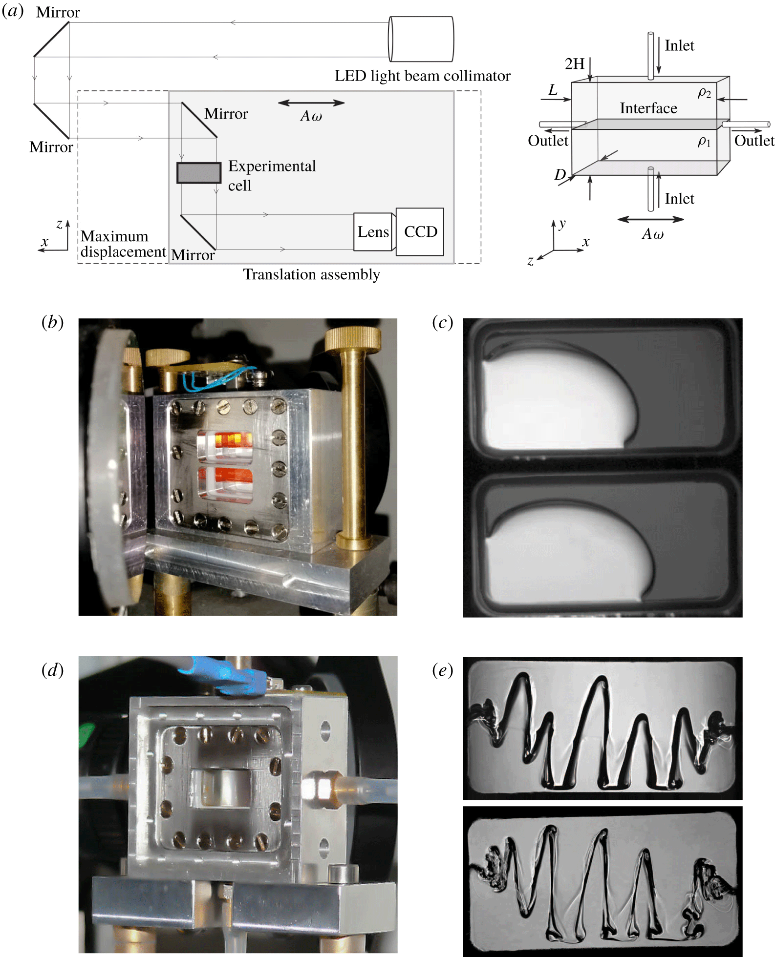
The microgravity experiments are performed in cuboidal containers of interior dimension  $L\times 2H\times D=15~\text{mm}\times 7.5~\text{mm}\times 5~\text{mm}$ (see figure 1a). The two large faces with area
 $L\times 2H$ are made of transparent quartz glass (Hellma) to allow observation of the fluids in the interior. The remaining boundaries are made from aluminium alloy, with a hole drilled through each; the holes in the upper and lower walls are used to fill the container, while those in the lateral walls are for drainage.
(a) Schematic view of the optical set-up (left) and the experimental cell (right). (b,d) Images of the experimental cells holding immiscible and miscible liquids, respectively. (c,e) Unprocessed cropped images showing the interface in reduced gravity. (c) Unforced immiscible combinations (see table 1)  $\text{I}_{a}$ (upper container) and
 $\text{I}_{b}$ (lower container); the lighter regions of the image correspond to FC-40 and the darker regions to silicone oil. (e) Miscible liquids under horizontal (
 $x$ axis) forcing: mixture
 $\text{M}_{a}$ (upper snapshot) and
 $\text{M}_{b}$ (lower snapshot).

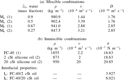
The experimental containers hold selected combinations of miscible or immiscible liquids, whose relevant physical properties are given in table 1. In the miscible experiments, two layers of water–isopropanol with different concentrations are used. The initial concentrations (mass fractions) of water in the two miscible layers were either 0.9 and 0.6 (mixture  $\text{M}_{a}$ in table 1), or 0.67 and 0.27 (mixture
 $\text{M}_{b}$ in table 1). In the immiscible experiments, two different silicone oils (
 $2$ and
 $20~\text{cSt}$) are used in combination with FC-40, a denser fluorocarbon oil. These immiscible combinations (respectively,
 $\text{I}_{a}$ and
 $\text{I}_{b}$ in table 1) have similar density ratios and interfacial tension, but differ by a factor of 10 in the viscosity ratio.
Physical properties of the experimental fluids at  $25\,^{\circ }\text{C}$. (a) Miscible water–isopropanol combinations: density
 $\unicode[STIX]{x1D70C}$, kinematic viscosity
 $\unicode[STIX]{x1D708}$ and diffusion coefficient
 $D$ (from Mialdun et al. Reference Mialdun, Yasnou, Shevtsova, Königer, Köhler, Alonso De Mezquia and Bou-Ali2012). (b) Immiscible combinations of FC-40 (Flourinert Liquids™) and silicone oil: density
 $\unicode[STIX]{x1D70C}$, kinematic viscosity
 $\unicode[STIX]{x1D708}$ and surface tension
 $\unicode[STIX]{x1D70E}$ (from Someya & Munakata Reference Someya and Munakata2005).

The position of the interface is monitored through (one of) the transparent sides of the container. In the immiscible case, the silicone oil is coloured with the additive Sudan IV so that its transparency is different from that of FC-40 (see figure 1b). The two liquids thus appear with different shading when illuminated from behind, as seen in the greyscale images of figure 1(c). In the miscible experiments, the interface is revealed using a shadowgraphy technique based on the variation of refractive index with concentration. Refraction caused by the large gradient across the interface makes it appear dark, as seen in the images of figure 1(e).
The image acquisition system uses light from a collimated light-emitting diode source, which is directed towards the experimental cell by a series of three mirrors. The image of the liquids and their interface is redirected by a final mirror before passing through a set of lenses to adjust the field of view and resolution (see figure 1a and Gaponenko et al. (Reference Gaponenko, Torregrosa, Yasnou, Mialdun and Shevtsova2015a) for more details). The CCD camera is set to record images at 48 or 80 frames per second. The higher rate is used for all experiments with immiscible liquids and provides very good resolution of interfacial waves at low or moderate frequencies. Even at higher forcing frequencies, there is no practical difficulty with stroboscopic effects since the frequencies of the relevant interfacial modes are known. At the highest forcing frequency where oscillatory interfacial waves were recorded ( $40~\text{Hz}$), there are enough points (two and four, respectively) to clearly distinguish harmonic from subharmonic waves.
The experimental cell, along with the lenses and camera, is mounted on a translation assembly attached to a linear motor that drives oscillations along the  $x$ axis (the lengthwise dimension
 $L$) at the selected frequency
 $\unicode[STIX]{x1D714}=2\unicode[STIX]{x03C0}f$ and amplitude
 $A$. The position of the motor is recorded by an encoder, which can be compared with the setting of the control software for calibration. The experiments using miscible liquids cover frequency and amplitude ranges of
 $2{-}24~\text{Hz}$ and 1.5–16 mm, respectively, while the experiments with immiscible liquids cover frequency and amplitude ranges of 5–50 Hz and 1–5.3 mm. Viewed from a reference frame attached to the container, the vibrated fluids are subjected to an effective gravity
 $\boldsymbol{G}(t)$ given by
 $$\begin{eqnarray}\displaystyle \boldsymbol{G}(t)=\boldsymbol{g}(t)+A\unicode[STIX]{x1D714}^{2}\cos (\unicode[STIX]{x1D714}t)\hspace{2.22198pt}\boldsymbol{i}, & & \displaystyle\end{eqnarray}$$
where  $\boldsymbol{i}$ is the unit vector along the
 $x$ axis. Note that, for convenience, we will continue to refer to the
 $x$ direction as ‘horizontal’ in microgravity, and to the two container boundaries parallel to the
 $x$ axis as the ‘upper’ and ‘lower’ walls.
The microgravity experiments were conducted during the 59th and 62nd ESA Parabolic Flight campaigns, which provided repeated periods of reduced gravity lasting approximately 22 s (forcing was applied for 15 s). The residual gravity level during this period satisfies (Pletser et al. Reference Pletser, Rouquette, Friedrich, Clervoy, Gharib, Gai and Mora2016)
 $$\begin{eqnarray}\displaystyle |g_{x,z}|\leqslant 0.01\,g_{0},\quad |g_{y}|\leqslant 0.05\,g_{0}, & & \displaystyle\end{eqnarray}$$
where  $g_{0}=9.81~\text{m}~\text{s}^{-2}$ and the
 $x,y,z$ subscripts refer to the coordinate axes shown in figure 1(a). Conditions on the flight were nearly isothermal during the experimental campaign, as confirmed by a negative temperature coefficient thermistor placed in the experimental cells. Over a full (daily) set of 31 parabolas, the temperature only increased by approximately
 $2\,^{\circ }\text{C}$. This justifies neglecting the variation of fluid properties with temperature, which is done in the simulations discussed below.
With miscible liquids, the diffusive interface naturally thickens during the experiments. Gaponenko et al. (Reference Gaponenko, Mialdun and Shevtsova2018) considered the effect of initial interface thickness on pattern selection after the frozen wave instability and found that a more diffuse interface promotes patterns of smaller wavenumber due to the reduced shear force. In the absence of convection, the mixing of the two liquids is slow and driven by diffusion. Vibrations strongly enhance mixing, to the extent that the interface thickens noticeably on a time scale of several seconds in the present experiments.
In order to have nearly constant initial conditions, a filling procedure is used to reinitialize the interface between experiments in the miscible case. Both liquids are injected simultaneously at an optimized flow rate by two identical pumps through the inlets on the upper and lower walls. Upon completion of the experiment, the liquids are drained through the lateral outlets. Flexible tubes (see figure 1d) connect the inlets with the filling system and the outlets with a waste bag; these do not constrain the mechanical vibration of the container. Valves are used to isolate the experimental cell and prevent interaction with the fluid in the tubes (Gaponenko et al. Reference Gaponenko, Torregrosa, Yasnou, Mialdun and Shevtsova2015a).
Experiments are characterized by the properties of the liquids used, by the forcing applied (frequency and amplitude) and by the start time of this forcing, i.e. whether vibrations begin during the hypergravity or microgravity portion of the given parabolic manoeuvre. If vibrations are initiated in hypergravity, the initial interface is relatively flat, although its orientation may not be completely parallel to the vibrational axis. If the vibrations are initiated during the microgravity period, then the interface has some time to move prior to forcing. With miscible liquids, the typical result of this is an increase in the average angle of the interface, which leads to a qualitative change in the interfacial pattern selected after forcing is applied.
The behaviour of immiscible liquids in microgravity is different due to interfacial tension, which causes the unforced interface to take a drop-like shape (partly attached to the walls); see figure 1(c). Such an interface cannot be well characterized by an average angle. The simulations of immiscible liquids presented in this paper are therefore not intended to reproduce the experiments initiated in microgravity, but rather to generalize and compare with those for miscible liquids and to complement results of Salgado Sánchez et al. (Reference Salgado Sánchez, Gaponenko, Porter and Shevtsova2019a), where pattern selection in finite containers was considered when starting from a perfectly flat (horizontal) interface.
Further details of the experimental set-up and observed interfacial phenomena can be found in Salgado Sánchez et al. (Reference Salgado Sánchez, Yasnou, Gaponenko, Mialdun, Porter and Shevtsova2019b) and Gaponenko et al. (Reference Gaponenko, Torregrosa, Yasnou, Mialdun and Shevtsova2015a).
2.2 Experimental results
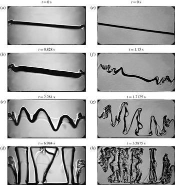
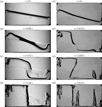
The development of the frozen wave instability in miscible liquids is shown via four snapshots in figures 2 and 3, with mixture  $\text{M}_{a}$ (see table 1) in panels (a–d) and mixture
 $\text{M}_{b}$ in panels (e–h). For each mixture, the experiments in those two figures are performed with identical vibrational velocities but differ in whether the forcing starts during hypergravity (figure 2) or during microgravity (figure 3). The different orientations of the initial interface (just prior to forcing) that result from this choice have a marked effect on the final pattern shown in panels (d,h).
Snapshots (times labelled) showing the temporal evolution of the frozen wave instability in miscible layers subjected to horizontal vibrations starting from a slightly tilted interface. (a–d) Mixture  $\text{M}_{a}$ of table 1 with
 $f=14~\text{Hz}$,
 $A=2.5~\text{mm}$ (
 $A\unicode[STIX]{x1D714}=219.9~\text{mm}~\text{s}^{-1}$) and initial angle
 $\unicode[STIX]{x1D6FC}\approx 4.5^{\circ }$. (e–h) Mixture
 $\text{M}_{b}$ of table 1 with
 $f=8~\text{Hz}$,
 $A=11~\text{mm}$ (
 $A\unicode[STIX]{x1D714}=552.9~\text{mm}~\text{s}^{-1}$) and initial angle
 $\unicode[STIX]{x1D6FC}\approx 5.0^{\circ }$. Microgravity begins at
 $t\approx 0.75~\text{s}$ and
 $t\approx 1.2~\text{s}$, respectively, for these experiments.

Snapshots (times labelled) showing the temporal evolution of the frozen wave instability in miscible layers subjected to horizontal vibrations starting from a more tilted interface. (a–d) Mixture  $\text{M}_{a}$ of table 1 with
 $f=12~\text{Hz}$,
 $A=2.91~\text{mm}$ (
 $A\unicode[STIX]{x1D714}=219.4~\text{mm}~\text{s}^{-1}$) and initial angle
 $\unicode[STIX]{x1D6FC}\approx 27^{\circ }$. (e–h) Mixture
 $\text{M}_{b}$ of table 1 with
 $f=8~\text{Hz}$,
 $A=11~\text{mm}$ (
 $A\unicode[STIX]{x1D714}=552.9~\text{mm}~\text{s}^{-1}$) and initial angle
 $\unicode[STIX]{x1D6FC}\approx 15^{\circ }$. These initial angles are measured in (b) and (e), respectively. The apparent breaks in the interface in (c,f) are optical effects.

When forcing begins prior to the microgravity portion of a parabolic manoeuvre, as in figure 2, the initial interface (see panels a,e) is flat and only slightly tilted (approximately  $5^{\circ }$). Depending on the specific profile of
 $\boldsymbol{g}(t)$, some features of the frozen wave growth under gravity may be visible. In figure 2(f), which shows the initial small-amplitude waves, the triangular waveform typical of the instability in gravity (Gaponenko & Shevtsova Reference Gaponenko and Shevtsova2016) can be seen since the transition to microgravity in this experiment has not yet occurred (it happens between panels (f) and (g) at
 $t\approx 1.20~\text{s}$). This contrasts with the small-amplitude waves in figure 2(c), which have more rounded crests since the microgravity period for this experiment begins, approximately, with panel (b) at
 $t\approx 0.75~\text{s}$. Furthermore, a portion of the interface near the endwalls displays a ‘fish spine’ type of pattern, as described in Shevtsova et al. (Reference Shevtsova, Gaponenko, Yasnou, Mialdun and Nepomnyashchy2015), related to nonlinear effects when
 $A\sim H$.
The formation of columns spanning the height of the container is common to both mixtures, as seen panels (d,h). The differences in the final (long-lived) patterns can be attributed mainly to the different applied vibrational velocity, which is the main control parameter of the frozen wave instability (Lyubimov & Cherepanov Reference Lyubimov and Cherepanov1986) and selects the wavenumber (number of columns) in the absence of gravity (Lyubimova et al. Reference Lyubimova, Ivantsov, Garrabos, Lecoutre, Gandikota and Beysens2017); this can be extended to the miscible case if the diffusive interface is thin, behaving as if it had finite (small) interfacial tension (Lacaze et al. Reference Lacaze, Guenoun, Beysens, Delsanti, Petitjeans and Kurowski2010).
After the formation of columns, large portions of the interface are nearly perpendicular to the applied forcing and subharmonic Faraday waves may be excited on them (Shevtsova et al. Reference Shevtsova, Gaponenko, Yasnou, Mialdun and Nepomnyashchy2016). This secondary instability, which can be seen most clearly in panel (h), produces an interfacial structure with two length and time scales: quasisteady columns spanning the container height, originating in the frozen wave instability, and subharmonic standing waves on the column walls, resulting from the Faraday instability. These two-scale patterns were observed in the recent experiments of Shevtsova et al. (Reference Shevtsova, Gaponenko, Yasnou, Mialdun and Nepomnyashchy2016) and, in the case of immiscible liquids, by Salgado Sánchez et al. (Reference Salgado Sánchez, Yasnou, Gaponenko, Mialdun, Porter and Shevtsova2019b).
Faraday waves can occur even in the absence of both gravity and surface tension since during half of the forcing period the surface is susceptible to the Rayleigh–Taylor instability, while in the other half there is an inertial restoring force. The threshold (Shevtsova et al. Reference Shevtsova, Gaponenko, Yasnou, Mialdun and Nepomnyashchy2016) depends on density and viscosity:
 $$\begin{eqnarray}\displaystyle A=\frac{2}{\unicode[STIX]{x1D70C}_{1}-\unicode[STIX]{x1D70C}_{2}}\sqrt{\frac{(\unicode[STIX]{x1D70C}_{1}+\unicode[STIX]{x1D70C}_{2})(\unicode[STIX]{x1D70C}_{1}\unicode[STIX]{x1D708}_{1}+\unicode[STIX]{x1D70C}_{2}\unicode[STIX]{x1D708}_{2})}{\unicode[STIX]{x1D714}}}. & & \displaystyle\end{eqnarray}$$
Here the subscripts  $1$ and
 $2$ refer to the lower and upper fluids, respectively. Using the values from table 1, equation (2.3) gives
 $8.6~\text{mm}$ for mixture
 $\text{M}_{a}$ at
 $12~\text{Hz}$ and
 $10.3~\text{mm}$ for mixture
 $\text{M}_{b}$ at
 $8~\text{Hz}$. These estimates are consistent with figure 2 in that subharmonic waves are not seen for mixture
 $\text{M}_{a}$ at
 $A=2.5~\text{mm}$, while they are seen for mixture
 $\text{M}_{b}$ at
 $A=11~\text{mm}$.
When Faraday waves are excited on the sides of a column, they propel the interface back and forth during each oscillation period. This process gradually deforms the interface as waves interact with those on neighbouring column walls, or with the remnants of the interface (density gradients) left behind by previous wave cycles on the same column. This latter interaction tends to generate spike-like formations, which can be be seen in figure 2(h) and, for numerical simulations, in figure 6(a,b) at  $t=3~\text{s}$. As this type of mixing proceeds, the waves gradually decay and disappear, leaving a more diffuse interface (compared to the case without surface waves). It is clear that, although parabolic flight experiments cannot properly investigate this slow process, the columnar structure itself will eventually be destroyed by diffusion as well.
When forcing begins in the microgravity period of a parabolic flight, as in figure 3, the unforced interface may rotate towards a more oblique orientation, particularly due to the balance of residual gravity components in the  $x$ and
 $y$ directions, as seen in panels (a,e). Even after forcing begins, the interface remains relatively flat at first (see panels b,f) without the clear frozen wave growth observed in figure 2. Instead, the vibration promotes continued rotation of the interface and an associated mean flow (see § 4.1.1 for details). While the lateral portions of the interface bend along the upper and lower boundaries, the central portion continues to rotate towards a vertical orientation, sometimes overshooting somewhat (panels c,g) before settling into a long-lived final state with the two liquids basically occupying opposite sides of the container (panels d,h). This final state is consistent with vibroequilibria theory (Gavrilyuk, Lukovsky & Timokha Reference Gavrilyuk, Lukovsky and Timokha2004; Fernández et al. Reference Fernández, Salgado Sánchez, Tinao, Porter and Ezquerro2017a,Reference Fernández, Tinao, Porter and Laveron-Simavillab), which, if gravity and surface tension are neglected, selects density contours perpendicular to the vibrational forcing.
Note that auxiliary frozen waves often develop during the latter stages of column development along the horizontal portions of the interface that lie close to the upper and lower walls. Their evolution is analogous to the frozen wave growth explained above, but with thinner columns (fingers) that may not reach the top/bottom.
Among other things, it is apparent from the experimental results discussed above that the initial surface orientation has a crucial influence on the dynamics of the interface and the structure that eventually develops. In the remainder of this paper, we use numerical simulations to systematically investigate the effect of initial orientation on pattern selection in both miscible and immiscible liquids.
3 Mathematical formulation and numerical models
This section summarizes the equations and numerical methods used to simulate the vibrated liquids and follow the dynamics of the interface separating them. The simulations, for both miscible and immiscible liquids, are performed in a two-dimensional rectangular domain, a simplification that is justified by the following considerations.
The basic frozen wave instability produces two-dimensional patterns with a wavenumber aligned with the projection of the forcing axis along the interface. In the absence of certain secondary instabilities (see e.g. Jalikop & Juel Reference Jalikop and Juel2012), there is no dependence on the cross-wise direction. This was generally found to be true of the experimental patterns as well, with the main exception being the appearance of disordered three-dimensional patterns related to vigorous drop ejection at high forcing amplitude (Salgado Sánchez et al. Reference Salgado Sánchez, Yasnou, Gaponenko, Mialdun, Porter and Shevtsova2019b), a situation that is not considered here. The two-dimensional numerical model used for the immiscible case was shown (Salgado Sánchez et al. Reference Salgado Sánchez, Gaponenko, Porter and Shevtsova2019a,Reference Salgado Sánchez, Yasnou, Gaponenko, Mialdun, Porter and Shevtsovab) to reproduce the main features of the fluid behaviour related to frozen waves and Faraday waves, which are the dominant phenomena in the microgravity experiments of interest. For the case of miscible fluids, the two-dimensional nature of the interfacial patterns was confirmed by a direct comparison with three-dimensional simulations (Gaponenko et al. Reference Gaponenko, Torregrosa, Yasnou, Mialdun and Shevtsova2015a).
Curvature in the transverse direction and capillary waves are also generally negligible. In microgravity environments, applied vibrations induce (Douady Reference Douady1990) capillary phenomena on the length scale  $l_{c}\sim \sqrt{\unicode[STIX]{x1D70E}/\unicode[STIX]{x1D70C}(A\unicode[STIX]{x1D714}^{2})}$. For the immiscible liquid layers of table 1, the interfacial tension
 $\unicode[STIX]{x1D70E}\sim 10^{-3}~\text{N}~\text{m}^{-1}$ is relatively small, making
 $l_{c}\lesssim 1~\text{mm}$. Meniscus effects were inappreciable in the experiments, where the selected patterns were manifestly two-dimensional. For the experiments with miscible liquids, conducted on a time scale of tens of seconds, the gradients at the diffusive interface remain large enough to act as a type of effective interfacial tension. As discussed in Gaponenko et al. (Reference Gaponenko, Torregrosa, Yasnou, Mialdun and Shevtsova2015a), the estimated interfacial tension of
 $\unicode[STIX]{x1D70E}\sim 10^{-6}~\text{N}~\text{m}^{-1}$ gives a very small
 $l_{c}$. Again, two-dimensional behaviour was clearly observed in the experiments, as well as in the three-dimensional simulations (Gaponenko et al. Reference Gaponenko, Torregrosa, Yasnou, Mialdun and Shevtsova2015a).
3.1 Miscible case
The two miscible liquids are assumed to be incompressible and to occupy equal volumes in the rectangular domain of figure 4. The parameters of the liquids are those given for mixtures  $\text{M}_{a}$ and
 $\text{M}_{b}$ in table 1.
Let  $\tilde{c}$ be the mass fraction of water and denote the initial concentrations in the
 $i$th layer as
 $\tilde{c}_{0i},\hspace{2.22198pt}i=1,2$ (lower and upper layers, respectively). Regardless of the mixture used, we may use a rescaled relative concentration
 $C$,
 $$\begin{eqnarray}\displaystyle C=\frac{\tilde{c}-\tilde{c}_{02}}{\tilde{c}_{01}-\tilde{c}_{02}},\quad 0\leqslant C\leqslant 1, & & \displaystyle\end{eqnarray}$$
which varies between  $0$ (initial upper layer) and
 $1$ (initial lower layer). Both fluid density and viscosity depend on the concentration of the mixture. For the experiments of § 2 using mixtures
 $\text{M}_{a}$ and
 $\text{M}_{b}$ (see table 1), the density differences are not large, which justifies the use of a linear approximation for this dependence (Mialdun et al. Reference Mialdun, Yasnou, Shevtsova, Königer, Köhler, Alonso De Mezquia and Bou-Ali2012):
 $$\begin{eqnarray}\displaystyle \unicode[STIX]{x1D70C}=\unicode[STIX]{x1D70C}_{2}\,(1-\unicode[STIX]{x1D6FD}_{\unicode[STIX]{x1D70C}}\,C),\quad \unicode[STIX]{x1D6FD}_{\unicode[STIX]{x1D70C}}=(\unicode[STIX]{x1D70C}_{2}-\unicode[STIX]{x1D70C}_{1})/\unicode[STIX]{x1D70C}_{2}, & & \displaystyle\end{eqnarray}$$
where  $\unicode[STIX]{x1D6FD}_{\unicode[STIX]{x1D70C}}=-0.0870$ for mixture
 $\text{M}_{a}$ and
 $-0.110$ for mixture
 $\text{M}_{b}$. Viscosity
 $\unicode[STIX]{x1D707}$, on the other hand, has a maximum at
 $\tilde{c}_{0}=0.5$ (Mialdun et al. Reference Mialdun, Yasnou, Shevtsova, Königer, Köhler, Alonso De Mezquia and Bou-Ali2012). For experiments using mixture
 $\text{M}_{a}$, we assume linear dependence:
 $$\begin{eqnarray}\displaystyle \unicode[STIX]{x1D707}=\unicode[STIX]{x1D707}_{2}\,(1-\unicode[STIX]{x1D6FD}_{\unicode[STIX]{x1D707}}\,C),\quad \unicode[STIX]{x1D6FD}_{\unicode[STIX]{x1D707}}=(\unicode[STIX]{x1D707}_{2}-\unicode[STIX]{x1D707}_{1})/\unicode[STIX]{x1D707}_{2}, & & \displaystyle\end{eqnarray}$$
where  $\unicode[STIX]{x1D6FD}_{\unicode[STIX]{x1D707}}=0.538$, since the region of interest of concentration is
 $0.5\leqslant \tilde{c}_{0}\leqslant 0.9$. In experiments with mixture
 $\text{M}_{b}$, the viscosity is approximated (Mialdun et al. Reference Mialdun, Yasnou, Shevtsova, Königer, Köhler, Alonso De Mezquia and Bou-Ali2012) using the fourth-order polynomial
 $$\begin{eqnarray}\displaystyle \unicode[STIX]{x1D707}=(0.3719\,C^{4}+1.0456\,C^{3}+0.5679\,C^{2}+1.2344\,C+2.7208)\times 10^{-3}~\text{Pa}~\text{s}, & & \displaystyle\end{eqnarray}$$
which provides the values for  $\text{M}_{b}$ (2) and
 $\text{M}_{b}$ (1) given in table 1 (using
 $\unicode[STIX]{x1D707}=\unicode[STIX]{x1D70C}\,\unicode[STIX]{x1D708}$) when
 $C=0$ and
 $1$, respectively.
Miscible simulations are performed in a domain of length  $L$ and height
 $2H$. Vibrations of frequency
 $\unicode[STIX]{x1D714}$ and amplitude
 $A$ are applied in the
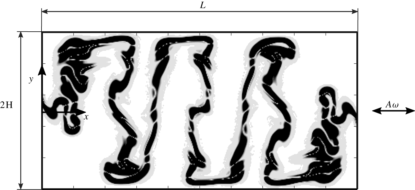
 $x$ direction. A solution is shown for illustration (the interface appears dark).

The effective interfacial tension at the diffusive interface is several orders of magnitude smaller than that of most immiscible liquids (Gaponenko et al. Reference Gaponenko, Torregrosa, Yasnou, Mialdun and Shevtsova2015a). It is thus neglected at leading order and the system is treated as a single layer with a variable concentration; the interface is located by the contour  $C=0.5$, which is a region of large concentration gradient.
With no residual (constant) gravity,  $\boldsymbol{g}=0$ in (2.1), the force experienced by the liquid is
 $$\begin{eqnarray}\displaystyle \boldsymbol{G}(t)=A\unicode[STIX]{x1D714}^{2}\cos (\unicode[STIX]{x1D714}t)\boldsymbol{i}, & & \displaystyle\end{eqnarray}$$
and momentum and mass transport equations read (Gaponenko et al. Reference Gaponenko, Torregrosa, Yasnou, Mialdun and Shevtsova2015a)
 $$\begin{eqnarray}\displaystyle & \displaystyle \unicode[STIX]{x1D70C}[\boldsymbol{u}_{t}+(\boldsymbol{u}\boldsymbol{\cdot }\unicode[STIX]{x1D735})\,\boldsymbol{u}]=-\unicode[STIX]{x1D735}p+\unicode[STIX]{x1D735}(\unicode[STIX]{x1D707}\,\unicode[STIX]{x1D735}\boldsymbol{u})+\unicode[STIX]{x1D70C}\hspace{2.22198pt}\boldsymbol{G}(t), & \displaystyle\end{eqnarray}$$
 $$\begin{eqnarray}\displaystyle & \displaystyle C_{t}+\boldsymbol{u}\boldsymbol{\cdot }\unicode[STIX]{x1D735}C=D\,\unicode[STIX]{x1D6FB}^{2}C, & \displaystyle\end{eqnarray}$$
 $$\begin{eqnarray}\displaystyle & \displaystyle \unicode[STIX]{x1D735}\boldsymbol{\cdot }\boldsymbol{u}=0, & \displaystyle\end{eqnarray}$$
 $\boldsymbol{u}$ is the fluid velocity,
 $p$ is the pressure and
 $D$ is the diffusion coefficient given in table 1. No-slip and impermeability conditions apply on the container walls:
 $$\begin{eqnarray}\displaystyle \boldsymbol{u}=0,\quad \unicode[STIX]{x2202}C/\unicode[STIX]{x2202}n=0, & & \displaystyle\end{eqnarray}$$
where  $\unicode[STIX]{x2202}/\unicode[STIX]{x2202}n$ denotes the normal derivative.
The initial flow is assumed to be quiescent at  $t=0$, with
 $\boldsymbol{u}=0$, while the concentration begins as a step function (see Gaponenko et al. Reference Gaponenko, Torregrosa, Yasnou, Mialdun and Shevtsova2015a):
 $$\begin{eqnarray}\displaystyle C_{0}(x,y)=\left\{\begin{array}{@{}ll@{}}0 & y-y_{0}(x)>0;\\ 1 & y-y_{0}(x)<0,\end{array}\right. & & \displaystyle\end{eqnarray}$$
where  $y_{0}$ is the interface location at
 $t=0$. The angle between the vibrational axis and the initial interface, locally given by
 $\tan ^{-1}(\text{d}y_{0}(x)/\text{d}x)$, is implicit in the choice of
 $y_{0}(x)$. We take a linear initial profile for
 $y_{0}(x)$ and vary this orientation between
 $0^{\circ }$ (parallel to the vibrational axis) and
 $30^{\circ }$.
The commercial solver FLUENT v.17.2 is used for solving (3.2)–(3.8) for mixtures  $\text{M}_{a}$ and
 $\text{M}_{b}$ in the two-dimensional domain of figure 4. Time dependence is treated using a standard implementation of the Pressure-Implicit with Splitting of Operators (PISO) pressure–velocity coupling scheme, while spatial discretization is done using the Pressure Staggering Options (PRESTO) technique for the pressure equation and a third-order Monotone Upstream-Centered Scheme for Conservation Laws (MUSCL) technique for the momentum and mass transport equations. Numerical convergence was considered in Gaponenko et al. (Reference Gaponenko, Torregrosa, Yasnou, Mialdun and Shevtsova2015a) and an orthogonal homogeneous discretization of
 $N_{x}\times N_{y}=400\times 200$ was selected, with
 $N_{x}$ and
 $N_{y}$ the number of mesh elements along the
 $x$ and
 $y$ axes, respectively. The maximum time step is set to
 $10^{-4}~\text{s}$ to satisfy the Courant–Friedrichs–Lewy (CFL) condition at small mesh sizes.
3.2 Immiscible case
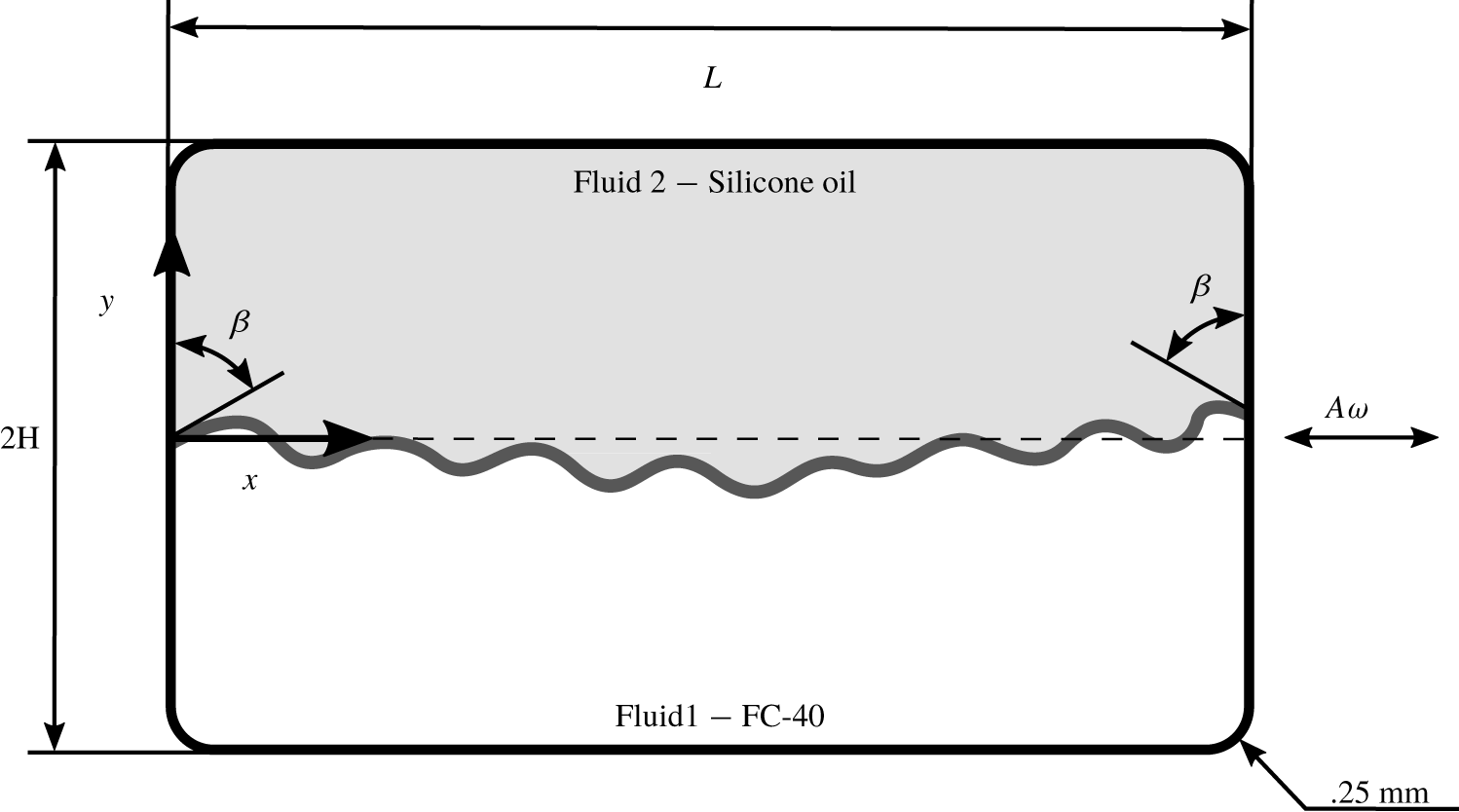
The two immiscible liquids are assumed to be incompressible and to occupy equal volumes of the rectangular domain shown in figure 5. The denser fluid is placed at the bottom so that the system is stable in the presence of gravity. Vibrations of amplitude  $A$ and frequency
 $\unicode[STIX]{x1D714}$ are again applied along the
 $x$ axis and the contact angle
 $\unicode[STIX]{x1D6FD}$ is set to
 $90^{\circ }$. Note that the corners of this domain are rounded, with a radius of 0.25 mm. This is done to match the experimental container, which was machined with a drill bit of this radius, and has the advantage of eliminating the numerically singular behaviour that would otherwise occur as the interface moves across a corner.
A level-set approach (Olsson & Kreiss Reference Olsson and Kreiss2005) is implemented for tracking the interface, with fluid properties defined as functions of the level-set variable  $\unicode[STIX]{x1D719}$, which obeys
 $$\begin{eqnarray}\displaystyle \unicode[STIX]{x1D719}_{t}+\unicode[STIX]{x1D735}\boldsymbol{\cdot }(\boldsymbol{u}\unicode[STIX]{x1D719})=\unicode[STIX]{x1D6FE}\unicode[STIX]{x1D735}\boldsymbol{\cdot }\left(\unicode[STIX]{x1D700}\unicode[STIX]{x1D735}\unicode[STIX]{x1D719}-\unicode[STIX]{x1D719}(1-\unicode[STIX]{x1D719})\frac{\unicode[STIX]{x1D735}\unicode[STIX]{x1D719}}{|\unicode[STIX]{x1D735}\unicode[STIX]{x1D719}|}\right). & & \displaystyle\end{eqnarray}$$
Here, the parameter  $\unicode[STIX]{x1D6FE}$ is set equal to the vibrational velocity
 $A\unicode[STIX]{x1D714}$, while
 $\unicode[STIX]{x1D700}$ is a small diffusive term added for numerical stability and taken to be of the order of the maximum mesh element size after convergence. A smoothed Heaviside step function
 ${\mathcal{H}}$ is defined (Salgado Sánchez et al. Reference Salgado Sánchez, Yasnou, Gaponenko, Mialdun, Porter and Shevtsova2019b) by
 $$\begin{eqnarray}\displaystyle {\mathcal{H}}(\unicode[STIX]{x1D719})=\left\{\begin{array}{@{}ll@{}}0,1 & \unicode[STIX]{x1D719}<-\unicode[STIX]{x1D700},\unicode[STIX]{x1D719}>\unicode[STIX]{x1D700}\\[2.0pt] {\displaystyle \frac{1}{2}}+{\displaystyle \frac{\unicode[STIX]{x1D719}}{2\unicode[STIX]{x1D700}}}+{\displaystyle \frac{1}{2\unicode[STIX]{x03C0}}}\sin \left({\displaystyle \frac{\unicode[STIX]{x03C0}\unicode[STIX]{x1D719}}{\unicode[STIX]{x1D700}}}\right) & |\unicode[STIX]{x1D719}|\leqslant \unicode[STIX]{x1D700},\end{array}\right. & & \displaystyle\end{eqnarray}$$
and is used to write the density  $\unicode[STIX]{x1D70C}$ and viscosity
 $\unicode[STIX]{x1D707}$ as
 $$\begin{eqnarray}\displaystyle & \displaystyle \unicode[STIX]{x1D70C}=\unicode[STIX]{x1D70C}_{1}+(\unicode[STIX]{x1D70C}_{2}-\unicode[STIX]{x1D70C}_{1}){\mathcal{H}}, & \displaystyle\end{eqnarray}$$
 $$\begin{eqnarray}\displaystyle & \displaystyle \unicode[STIX]{x1D707}=\unicode[STIX]{x1D707}_{1}+(\unicode[STIX]{x1D707}_{2}-\unicode[STIX]{x1D707}_{1}){\mathcal{H}}, & \displaystyle\end{eqnarray}$$
 $\unicode[STIX]{x1D719}=0,1$.
Sketch illustrating the immiscible numerical model: two superposed layers of immiscible liquids confined in a  $L\times 2H$ rectangular container, displaying a finite contact angle
 $\unicode[STIX]{x1D6FD}$ with the solid walls. The cell is subjected to vibrations of frequency
 $\unicode[STIX]{x1D714}$ and amplitude
 $A$ in the
 $x$ direction.

Equations (3.9)–(3.11) are solved together with the continuous incompressible Navier–Stokes equations (Kothe, Mjolsness & Torrey Reference Kothe, Mjolsness and Torrey1991)
 $$\begin{eqnarray}\displaystyle & \displaystyle \unicode[STIX]{x1D70C}[\boldsymbol{u}_{t}+(\boldsymbol{u}\boldsymbol{\cdot }\unicode[STIX]{x1D735})\boldsymbol{u}]=-\unicode[STIX]{x1D735}p+\unicode[STIX]{x1D735}(\unicode[STIX]{x1D707}\,\unicode[STIX]{x1D735}\boldsymbol{u})+\unicode[STIX]{x1D6FF}\,\boldsymbol{f}_{\unicode[STIX]{x1D70E}}+\unicode[STIX]{x1D70C}\,\boldsymbol{G}(t), & \displaystyle\end{eqnarray}$$
 $$\begin{eqnarray}\displaystyle & \displaystyle \unicode[STIX]{x1D735}\boldsymbol{\cdot }\boldsymbol{u}=0. & \displaystyle\end{eqnarray}$$
 $\boldsymbol{f}_{\unicode[STIX]{x1D70E}}$ term in the momentum equation:
 $$\begin{eqnarray}\displaystyle \boldsymbol{f}_{\unicode[STIX]{x1D70E}}=(\unicode[STIX]{x1D70E}\unicode[STIX]{x1D705})\,\boldsymbol{n},\quad \unicode[STIX]{x1D705}=\unicode[STIX]{x1D735}\boldsymbol{\cdot }\boldsymbol{n},\quad \boldsymbol{n}=\frac{\unicode[STIX]{x1D735}\unicode[STIX]{x1D719}}{|\unicode[STIX]{x1D735}\unicode[STIX]{x1D719}|}, & & \displaystyle\end{eqnarray}$$
where  $\unicode[STIX]{x1D705}$ is the curvature of the interface and
 $\boldsymbol{n}$ is the normal vector. These interfacial effects are localized by the prefactor
 $\unicode[STIX]{x1D6FF}$, which can be approximated in terms of the level-set function by
 $\unicode[STIX]{x1D6FF}=|\unicode[STIX]{x1D735}\unicode[STIX]{x1D719}|$.
Navier-slip boundary conditions, which introduce an artificial frictional force  $\boldsymbol{f}_{\unicode[STIX]{x1D708}}=(\unicode[STIX]{x1D707}/\unicode[STIX]{x1D6FF}_{\unicode[STIX]{x1D708}})\boldsymbol{u}$ to preserve contact angle
 $\unicode[STIX]{x1D6FD}$ while permitting contact line motion, are applied on all solid walls:
 $$\begin{eqnarray}\displaystyle \boldsymbol{u}\boldsymbol{\cdot }\boldsymbol{n}_{w}=0,\quad \boldsymbol{u}\boldsymbol{\cdot }[\unicode[STIX]{x1D70E}(\boldsymbol{n}_{w}-\boldsymbol{n}\cos \unicode[STIX]{x1D6FD})\unicode[STIX]{x1D6FF}]=0, & & \displaystyle\end{eqnarray}$$
where  $\boldsymbol{n}_{w}$ is the corresponding normal vector.
The applied acceleration is given by (2.1) while the initial velocity is zero throughout the domain. Because of numerical difficulties (related to contact angle) when starting from a prescribed initial interface, the different interface orientations are achieved by first allowing the unforced interface to relax with a fixed ratio of  $g_{x}/g_{y}$. The residual gravity is then gradually reduced (while maintaining the same ratio of
 $g_{x}/g_{y}$) until reaching a magnitude below
 $0.01\,g_{0}$. Since the corresponding capillary wavelength
 $\unicode[STIX]{x1D706}=2\unicode[STIX]{x03C0}\sqrt{\unicode[STIX]{x1D70E}/(\unicode[STIX]{x1D70C}_{1}-\unicode[STIX]{x1D70C}_{2})g}\geqslant 50~\text{mm}>L$, this level of residual gravity ensures that the critical wavelength is selected by the container size and the magnitude of the vibrational velocity (Salgado Sánchez et al. Reference Salgado Sánchez, Gaponenko, Porter and Shevtsova2019a,Reference Salgado Sánchez, Yasnou, Gaponenko, Mialdun, Porter and Shevtsovab); it has a negligible effect on pattern selection when compared to the ideal zero-gravity case.
After the fluid reaches a hydrostatic equilibrium in this manner, the forcing is activated. A transient time of 0.25 s is used in place of the parameter  $\unicode[STIX]{x1D700}$ in
 ${\mathcal{H}}(t)$ (see (3.10)) as a prefactor to smooth the onset of vibrations, as in Salgado Sánchez et al. (Reference Salgado Sánchez, Yasnou, Gaponenko, Mialdun, Porter and Shevtsova2019b). For the results presented below, we approximate the average interface orientation by measuring the slope in the centre of the container at the moment of forcing activation.
The commercial software COMSOL Multiphysics 5.3 was used for solving the governing two-dimensional equations. Convergence was tested previously in Salgado Sánchez et al. (Reference Salgado Sánchez, Yasnou, Gaponenko, Mialdun, Porter and Shevtsova2019b) for a similar configuration to select a maximum mesh size  $H/12.5$. A generalized-
 $\unicode[STIX]{x1D6FC}$ (Erlicher, Bonaventura & Bursi Reference Erlicher, Bonaventura and Bursi2002) integration scheme is used, which produces less numerical diffusion than the extended backward differentiation formulae schemes. The vibrated problem is initialized using a backward Euler method for one step. The maximum time step is set to
 $1/(10\,f)$ and is automatically reduced to satisfy the CFL stability condition using streamline (Harari & Hughes Reference Harari and Hughes1992) and cross-wind (Codina Reference Codina1993) stabilization techniques.
4 Numerical results
The results of a series of numerical simulations are presented in this section showing the effect of initial orientation on the dynamics of the interface as it evolves towards a quasisteady state. The final long-lived pattern is characterized by several complementary wavelength measurements.
4.1 Miscible liquids
A series of simulations using mixtures  $\text{M}_{a}$ and
 $\text{M}_{b}$ were performed in the rectangular domain of figure 4 with
 $L\times 2H=15~\text{mm}\times 7.5~\text{mm}$. Since the results were qualitatively similar, with the same type of dependence on initial inclination, only the (slightly clearer) results for mixture
 $\text{M}_{b}$ are presented here.
4.1.1 Pattern development for different initial angles
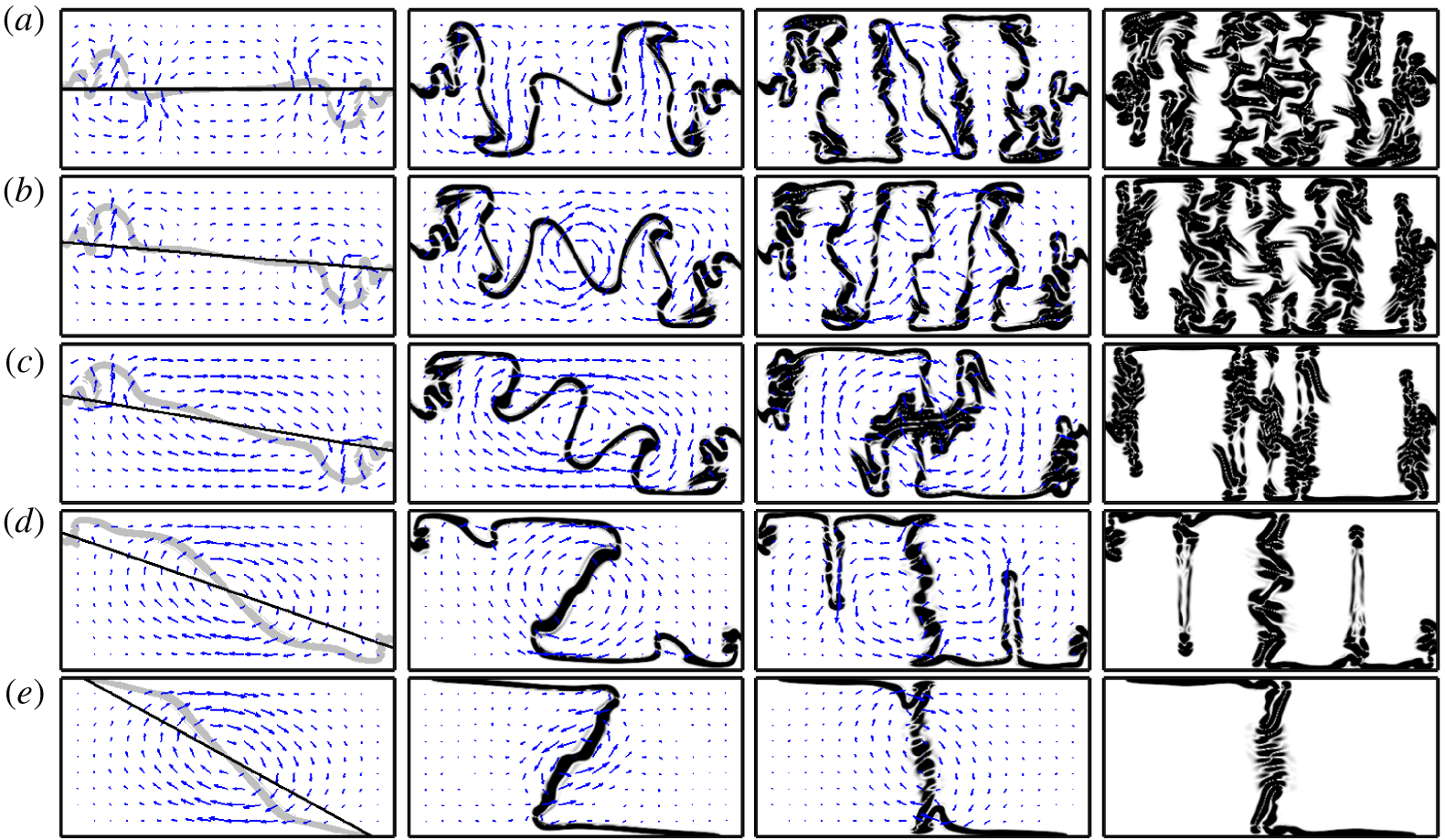
The results of five numerical simulations are shown in figure 6, which can be compared with the experimental results shown in figures 2(e–h) and 3(e–h). The same horizontal vibration is applied, with  $f=8~\text{Hz}$ and
 $A=11~\text{mm}$ (
 $A\unicode[STIX]{x1D714}=552.9~\text{mm}~\text{s}^{-1}$), while different initial interface orientations of
 $0^{\circ }$,
 $5^{\circ }$,
 $10^{\circ }$,
 $20^{\circ }$ and
 $30^{\circ }$ are used. The four snapshots in each row of figure 6 show the interface at
 $t=0.2~\text{s}$ (superimposed on the initial condition),
 $0.5~\text{s}$,
 $1~\text{s}$ and
 $3~\text{s}$. The mean velocity (averaged over two excitation periods) associated with the motion of the interface is also shown for the three earlier times, before the final quasisteady state is reached; note that the scale of the arrows is not preserved between panels.
Numerical simulations showing the temporal evolution of the frozen wave instability in mixture  $\text{M}_{b}$ with
 $f=8~\text{Hz}$ and
 $A=11~\text{mm}$ (
 $A\unicode[STIX]{x1D714}=552.9~\text{mm}~\text{s}^{-1}$) for increasing initial interface angles: (a)
 $0^{\circ }$, (b)
 $5^{\circ }$, (c)
 $10^{\circ }$, (d)
 $20^{\circ }$ and (e)
 $30^{\circ }$. The columns show snapshots at
 $t=0.2~\text{s}$,
 $0.5~\text{s}$,
 $1~\text{s}$ and
 $3~\text{s}$. The mean velocity field (averaged over two periods) is shown for the first three snapshots (arrow scale not maintained between panels); the solution at
 $t=3~\text{s}$ is quasisteady. The initial interface condition is shown in the leftmost panels at
 $t=0.2~\text{s}$ by a solid black line, while the interface is plotted in grey.

The evolution of the frozen wave instability from an initial horizontal interface, as illustrated in figure 6(a), was described by Gaponenko & Shevtsova (Reference Gaponenko and Shevtsova2016) for various gravity levels. Here, this case provides a reference to compare with the simulations initiated from a rotated interface. As soon as the forcing begins, approximately sinusoidal perturbations appear on the interface, most prominently near the lateral walls. These perturbations grow rapidly in the absence of strong gravity or surface tension to constrain them, and soon reach the upper and lower boundaries. The final long-lived structure takes the form of alternating columns. Note that the antisymmetric nature of the horizontal forcing – more precisely, the symmetry under horizontal reflection through the midline and translation by half a period of the forcing – is transmitted, in part, to the frozen wave structure. An investigation of similar structures in immiscible liquids (Salgado Sánchez et al. Reference Salgado Sánchez, Gaponenko, Porter and Shevtsova2019a) found that the symmetry of the final state depends on the container size as well as on the applied vibration. Although approximately symmetric patterns were found at moderate forcings, this symmetry can be lost as the ratio between the wavelength and the container length decreases.
When the initial interface is rotated by  $5^{\circ }$, as in the simulations of figure 6(b), the evolution of the frozen wave instability is not substantially different from the horizontal case, although there are subtle changes. Comparing the snapshots at
 $t=0.2~\text{s}$, one can see that the mean flow has more of a vertical component in figure 6(b), which indicates some rotation of this central portion of the interface. In this case, its effect is not strong enough to modify the final structure in a significant way.
As the angle of the initial interface is increased further to  $10^{\circ }$, as in the simulations of figure 6(c), the change in the mean flow is more obvious. In contrast to the horizontal and
 $5^{\circ }$ cases, the mean flow in the centre of the cell is now stronger than the vortical flow near the lateral walls associated with the growth of the frozen waves. The rotation of the central portion of the interface during this initial period does not prevent the growth of frozen waves, which are visible on the inclined interface at
 $t=0.5~\text{s}$. However, by
 $t=1~\text{s}$, its continued rotation disrupts the regular growth of these interior frozen waves (columns), twisting them before they can extend across the height of the container. The final quasisteady state contains several anomalous thin columns in the central region.
When the angle of the initial interface is  $20^{\circ }$, as in the simulations of figure 6(d), the rotation of the central portion of the interface is stronger and largely prevents the development of frozen waves into full columns. However, there are small perturbations along the horizontal portions of the interface, and two of these are noticeably enlarged at
 $t=0.5~\text{s}$. These humps, or fingers, grow slowly into thin columns, although they do not fully reach the opposite boundary during the observation time. Since these thin fingers are qualitatively different from the ‘primary’ frozen wave columns, they are considered auxiliary and are not included in the wavelength calculations presented below. Again, the pattern is approximately asymmetric with respect to horizontal reflection about the midline.
When the angle of the initial interface is  $30^{\circ }$, as in the simulations of figure 6(e), the central region rapidly rotates towards a vertical orientation, first overshooting this somewhat (see the snapshot at
 $t=0.5~\text{s}$ and the experiment in figure 3g), before settling into a final quasisteady state with each of the liquids (almost, but not completely) occupying one half of the container.
4.1.2 Wavenumber selection for different initial angles
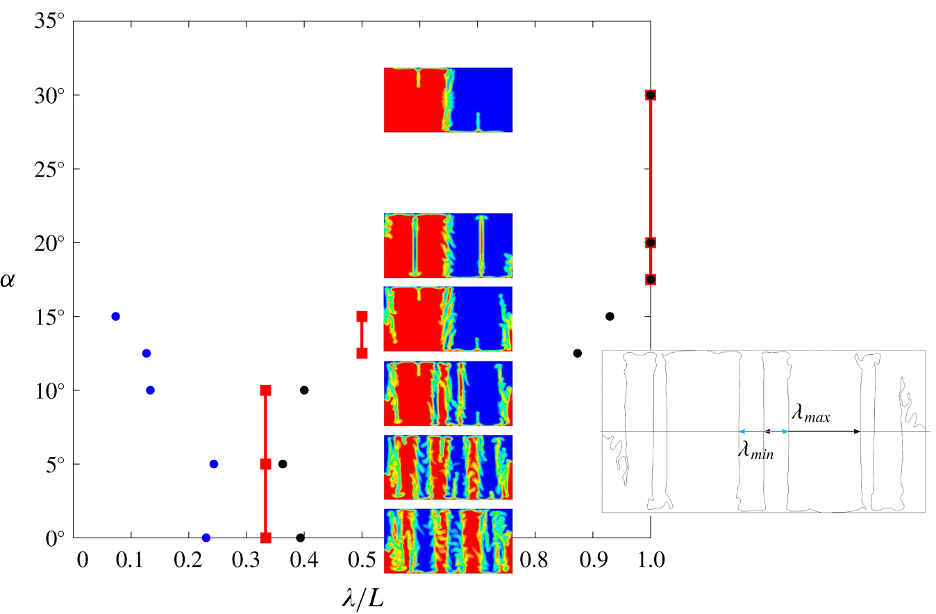
In figure 7 we represent the dependence of the final (long-lived) columnar structure on initial interface angle ( $\unicode[STIX]{x1D6FC}$) with three dimensionless wavelengths (
 $\unicode[STIX]{x1D706}/L$) measured along the midline
 $y=0$: the minimum (blue), maximum (black) and average (red), which is the same as the inverse number of paired columns. The location of the interface is taken as
 $C=0.5$. Snapshots showing the selected patterns for each angle are included, as is a sketch illustrating the calculation of minimum (
 $\unicode[STIX]{x1D706}_{min}$) and maximum (
 $\unicode[STIX]{x1D706}_{max}$) wavelengths.
Diagram showing three measured non-dimensional wavelengths  $\unicode[STIX]{x1D706}/L$ of the final quasisteady state versus initial interface angle
 $\unicode[STIX]{x1D6FC}$ (in degrees): minimum (blue), average (red) and maximum (black). The vibrational velocity is held constant at
 $A\unicode[STIX]{x1D714}=552.9~\text{mm}~\text{s}^{-1}$ (
 $f=8~\text{Hz}$,
 $A=11~\text{mm}$). Snapshots of the selected patterns are included, with the colourmap showing the concentration field (red for
 $C=0$, blue for
 $C=1$), as is a sketch illustrating how wavelengths are measured from the contour
 $C=0.5$. Note that the snapshots are taken after a longer time of
 $t=10~\text{s}$ so are slightly different from those at
 $t=3~\text{s}$ in figure 6.

For initial angles of  $10^{\circ }$ or less, the observed final states are qualitatively similar. Although the columns do change shape, the average wavenumber (half the number of abrupt concentration changes along the midline
 $y=0$) does not change. The changing shape of the columns is captured by the maximum and minimum wavelengths, which separate from each other as the angle
 $\unicode[STIX]{x1D6FC}$ increases. Qualitative transitions occur beyond
 $\unicode[STIX]{x1D6FC}\approx 10^{\circ }$, as the final pattern goes from one with three average wavelengths along the midline of the container, to one with two wavelengths at
 $\unicode[STIX]{x1D6FC}\approx 12.5^{\circ }$, to one with a single wavelength for
 $\unicode[STIX]{x1D6FC}\gtrsim 17.5^{\circ }$ (the thin fingers seen with
 $\unicode[STIX]{x1D6FC}=20^{\circ }$, for example, are not included in the wavelength measurement).
The type of pattern observed for inclinations of  $20^{\circ }$ and
 $30^{\circ }$ is the limiting one for large angles. Increasing the initial angle does not change the number of (large) columns, which remains at two, but does lead to a more rapid approach to the final state with its central vertical interface and, correspondingly, less time for any type of frozen wave column to develop. Auxiliary fingers and irregularities along the central boundary both diminish with greater initial inclination.
4.2 Immiscible liquids
The simulations of immiscible liquids were performed in the rectangular domain (with rounded corners) shown in figure 5. As in Salgado Sánchez et al. (Reference Salgado Sánchez, Gaponenko, Porter and Shevtsova2019a), we do not use the real viscosity of FC-40 given in table 1, but increase this to  $5~\text{cSt}$ in order to delay the onset of secondary Faraday waves. Otherwise, the parameters are those of combination
 $\text{I}_{b}$.
4.2.1 Pattern development for different initial angles
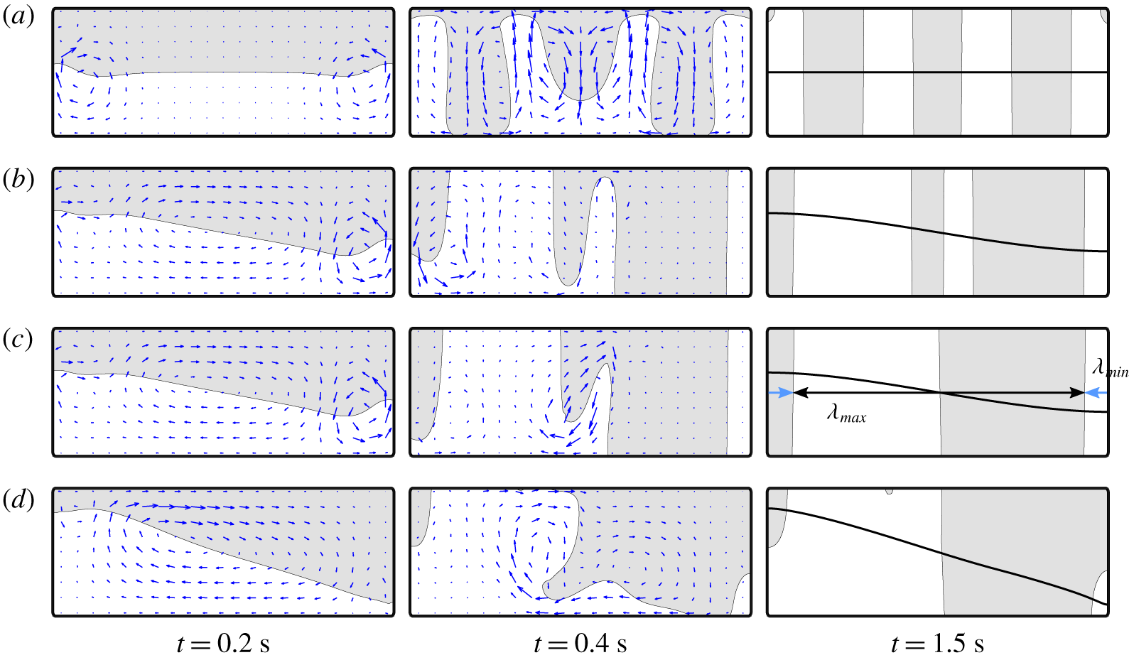
Figure 8 shows the evolution of the frozen wave instability in a rectangular cell of size  $L\times 2H=30~\text{mm}\times 7.5~\text{mm}$ for four initial interface orientations:
 $0^{\circ }$,
 $7^{\circ }$,
 $7.2^{\circ }$ and
 $14.15^{\circ }$. The amplitude and frequency are set at
 $A=1.5~\text{mm}$ and
 $f=45~\text{Hz}$. The mean velocity field (averaged over two excitation periods) is also shown for the two earlier snapshots, while the final image includes the initial interface for comparison.
Numerical simulations illustrating the development of the frozen wave instability in weightless condition in a  $L\times 2H=30~\text{mm}\times 7.5~\text{mm}$ container with
 $f=45~\text{Hz}$ and
 $A=1.5~\text{mm}$. The time of each snapshot is given under the corresponding column. The mean velocity (averaged over two excitation periods) is illustrated by scaled arrows (scale not preserved between panels) during the transient phase. The angle
 $\unicode[STIX]{x1D6FC}$ of the initial interface is varied: (a)
 $0^{\circ }$, (b)
 $7^{\circ }$, (c)
 $7.2^{\circ }$ and (d)
 $14.16^{\circ }$. The manner of calculating maximum (
 $\unicode[STIX]{x1D706}_{max}$) and minimum (
 $\unicode[STIX]{x1D706}_{\text{min}}$) wavelengths along the midline
 $y=0~\text{mm}$, used in figure 9, is illustrated for the final state of (c). The initial interface is shown (solid black curve) for comparison in the rightmost panels at
 $t=1.5~\text{s}$.

The development of the frozen wave instability from an initially flat horizontal interface, as illustrated in figure 8(a), was described in detail by Salgado Sánchez et al. (Reference Salgado Sánchez, Gaponenko, Porter and Shevtsova2019a). The pattern selection process was shown to be characterized by a cycle of column growth. The oscillatory vertical motion of the interface near the lateral boundaries creates a disturbance that tends to initiate the growth of frozen waves. Perturbations grow first near these walls, but propagate inward over time, as revealed by the horizontal component of the mean velocity at  $t=0.2~\text{s}$ (see also Dore (Reference Dore1973) and Shevtsova et al. (Reference Shevtsova, Gaponenko, Yasnou, Mialdun and Nepomnyashchy2015)). These frozen wave perturbations grow rapidly, approaching the upper and lower boundaries; see figure 8(a) at
 $t=0.4~\text{s}$. After slightly more time, they settle into quasisteady (nearly) vertical columns, as in the snapshot at
 $t=1.5~\text{s}$. Note the average left–right reflection symmetry of the solution in this case, both for the mean flow associated with the transient states and for the interface.
If the angle of the initial interface is increased slightly, the mean flow field changes substantially, as demonstrated in figure 8(b). Compared to the horizontal case ( $\unicode[STIX]{x1D6FC}=0^{\circ }$), where the mean flow in the centre of the cell is very small, there is for
 $\unicode[STIX]{x1D6FC}=7^{\circ }$ a significant vortical flow, which indicates a rotation of the central portion of the interface towards a perpendicular orientation with respect to the forcing axis, consistent with the theory of vibroequilibria. The rotation, however, is not fast enough to prevent the growth of some frozen waves into columns; see figure 8(b) at
 $t=0.4~\text{s}$. The final steady pattern, seen at
 $t=1.5~\text{s}$, contains two large columns and several smaller ones. Note that this selected interfacial structure has quite different symmetry compared to the horizontal case (
 $\unicode[STIX]{x1D6FC}=0^{\circ }$). In fact, it is approximately antisymmetric (or symmetric under inversion through the centre of the container and exchange of liquids), as were all of the solutions in figure 6 with miscible liquids.
Larger angles for the initial interface have the same effect as they did in figure 6, increasing the rotation rate of the central portion of the interface, as seen in the stronger mean flow, and reducing the time needed to reach the final state. The development of the frozen waves is hampered by this rotation. With  $\unicode[STIX]{x1D6FC}=7^{\circ }$, the two central perturbations are large enough to continue growing and form columns, but for
 $\unicode[STIX]{x1D6FC}=7.2^{\circ }$ they are reabsorbed by the larger columns before the final state is achieved. This marks a type of mode transition since the average wavenumber (i.e. number of paired columns) is reduced by one.
Figure 8(d) shows the evolution of the interface for  $\unicode[STIX]{x1D6FC}=14.16^{\circ }$. This case exhibits even more rotation of the central part of the interface and reduced development of thinner columns. The lateral perturbation seen near the right-hand wall in the previous three simulations at
 $t=0.2~\text{s}$, for example, is nearly gone. Although some FC-40 is trapped near the bottom right-hand corner, it is not enough to form a column, nor is the small mass of silicone oil in the upper left-hand corner. Further increase in
 $\unicode[STIX]{x1D6FC}$ will reduce the size of these regions even more, until
 $\unicode[STIX]{x1D6FC}$ becomes large enough that the contact points of the initial interface already reach the corners of the container without forcing. When this occurs, the evolution of the forced interface is driven by contact conditions, with the final pattern emerging after a complex dynamical process involving collisions between the interface and the upper and lower boundaries (Salgado Sánchez et al. Reference Salgado Sánchez, Gaponenko, Porter and Shevtsova2019a). In the simplest case, this process results in a final state with two columns, as with miscible liquids.
4.2.2 Wavenumber selection for different initial angles
The selection of the final columnar structure and its characteristic wavelength was considered for an initial horizontal interface by Salgado Sánchez et al. (Reference Salgado Sánchez, Gaponenko, Porter and Shevtsova2019a), where finite-size effects were investigated. In contrast to the continuous monotonic dependence of wavenumber on forcing predicted for an infinite inviscid system (Lyubimova et al. Reference Lyubimova, Ivantsov, Garrabos, Lecoutre, Gandikota and Beysens2017), the boundaries permit only discrete modes, which exist over finite forcing intervals separated by transitions related to the creation or destruction of new columns. Analogous but different types of mode transitions are observed if the initial angle  $\unicode[STIX]{x1D6FC}$ is varied rather than the the forcing.
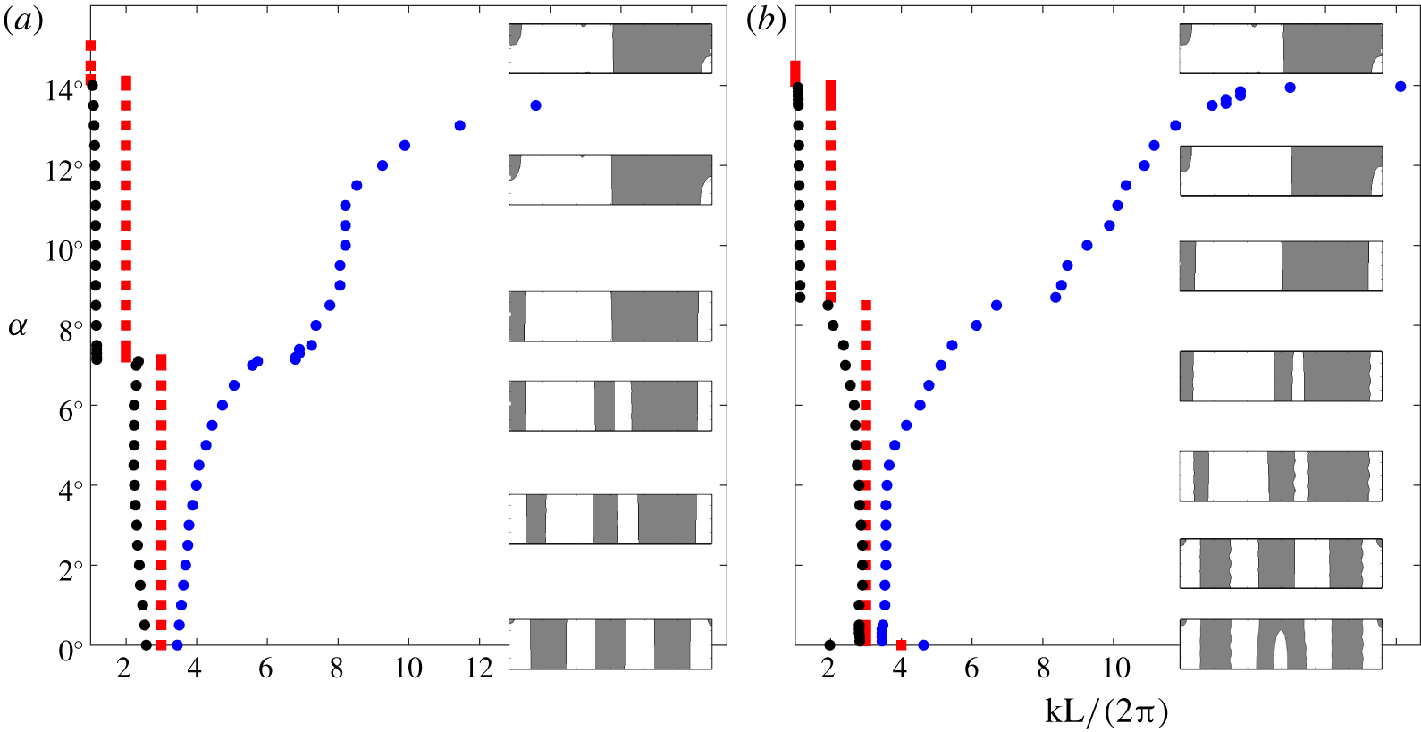
Diagrams showing the effect of initial interface angle  $\unicode[STIX]{x1D6FC}$ (in degrees) on dimensionless pattern wavenumber
 $kL/(2\unicode[STIX]{x03C0})$ (measured at
 $y=0$) for two applied vibrational velocities: (a)
 $A\unicode[STIX]{x1D714}=424~\text{mm}~\text{s}^{-1}$ (
 $f=45~\text{Hz}$,
 $A=1.5~\text{mm}$) and (b)
 $A\unicode[STIX]{x1D714}=565~\text{mm}~\text{s}^{-1}$ (
 $f=60~\text{Hz}$,
 $A=1.5~\text{mm}$). The domain measures
 $30~\text{mm}\times 7.5~\text{mm}$, with aspect ratio
 $\unicode[STIX]{x1D6E4}=4$. Three different wavenumbers are shown: minimum (black), average (red) and maximum (blue). Snapshots of the final selected patterns are included for illustration. The simulations used for (a) include those shown in figure 8.

The mode diagram presented in figure 9 shows three relevant non-dimensional wavenumbers measured along the midline  $y=0$ in the final steady structure: the minimum and maximum wavenumbers, and the averaged wavenumber, which gives the number of paired columns. These wavenumbers are shown over a range of initial interface angles between
 $0^{\circ }$ and
 $16^{\circ }$ in a
 $30~\text{mm}\times 7.5~\text{mm}$ container, i.e. with aspect ratio
 $\unicode[STIX]{x1D6E4}=L/(2H)=4$, and with two different vibrational velocities of
 $A\unicode[STIX]{x1D714}=424~\text{mm}~\text{s}^{-1}$ (figure 9a) and
 $565~\text{mm}~\text{s}^{-1}$ (figure 9b). Illustrative snapshots showing the final patterns are included for selected angles.
When  $\unicode[STIX]{x1D6FC}=0^{\circ }$, the final structure contains either three or four pairs of columns, depending on the applied forcing. Since these are not exactly the same length, the minimum and maximum wavelengths differ from the average value. For the higher vibrational velocity used in figure 9(b), the four-column pattern is observed only in the ideal
 $\unicode[STIX]{x1D6FC}=0$ case, with a transition to a three-column pattern observed when the initial inclination is increased to
 $\unicode[STIX]{x1D6FC}=0.1^{\circ }$.
As the initial inclination is increased, the difference between the maximum and minimum wavenumber grows until a mode transition (at  $\unicode[STIX]{x1D6FC}\simeq 7.15^{\circ }$ in figure 9a and
 $\unicode[STIX]{x1D6FC}\simeq 8.60^{\circ }$ in figure 9b) reduces the average wavenumber by one as the thin central columns fail to fully develop and are absorbed by their neighbours. The resulting mode has two thick central columns and two thin outer columns.
With a further increase in  $\unicode[STIX]{x1D6FC}$, these two outer columns grow thinner and, at some point, fail to span the height of the container. When (at
 $\unicode[STIX]{x1D6FC}\simeq 14.12^{\circ }$ in figure 9a and
 $\unicode[STIX]{x1D6FC}\simeq 14.16^{\circ }$ in figure 9b) these lateral fluid masses no longer extend enough to cross the midline
 $y=0$, the final mode transition to a single pair of columns is marked. Note that, although the location of the intermediate mode transition is delayed by higher vibrational velocity, the final mode transition is almost unaffected by the forcing amplitude.
To summarize, the orientation of the initial interface has a dramatic effect on the selected wavenumber (number of column pairs) of the final state. As in the case of miscible liquids, this results from the rotation of the central portion of the interface, consistent with vibroequilibria theory, and the corresponding reduction of the shear flow that drives the frozen wave (Kelvin–Helmholtz) instability.
4.2.3 Effect of the container aspect ratio
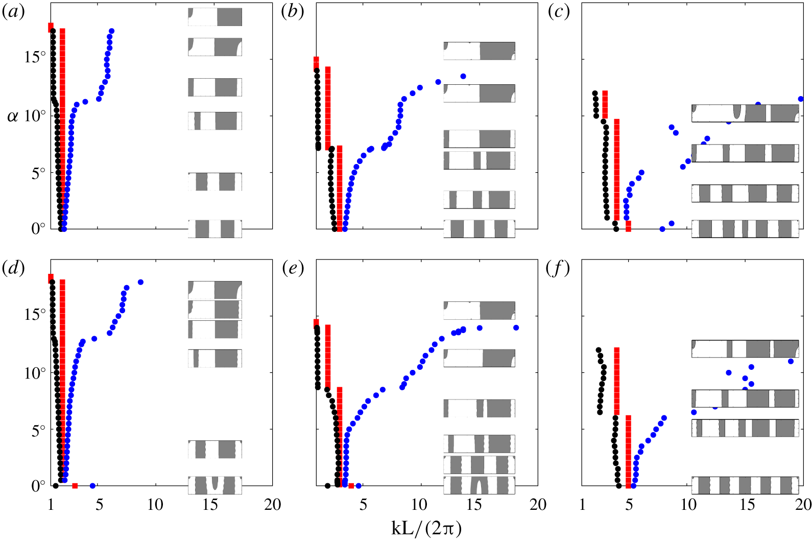
The orientation of the interface is a geometric feature that naturally relates to the aspect ratio of the container – since an interface inclined at a certain angle will cross the corners. This relationship is explored in figure 10, which shows the dependence on  $\unicode[STIX]{x1D6FC}$ of the pattern wavenumber for three different aspect ratios:
 $\unicode[STIX]{x1D6E4}=3$,
 $\unicode[STIX]{x1D6E4}=4$ and
 $\unicode[STIX]{x1D6E4}=6$. The same two vibrational velocities are applied as in figure 9 (a–c)
 $A\unicode[STIX]{x1D714}=424$ and (d–f)
 $565~\text{mm}~\text{s}^{-1}$.
Diagrams showing the effect of initial interface angle  $\unicode[STIX]{x1D6FC}$ (in degrees) on dimensionless pattern wavenumber
 $kL/(2\unicode[STIX]{x03C0})$ (measured at
 $y=0$) for different container aspect ratios: (a,d)
 $\unicode[STIX]{x1D6E4}=3$, (b,e)
 $\unicode[STIX]{x1D6E4}=4$ and (c,f)
 $\unicode[STIX]{x1D6E4}=6$. The minimum (black), average (red) and maximum (blue) wavenumbers are shown for each container at two different vibrational velocities: (a–c)
 $A\unicode[STIX]{x1D714}=424~\text{mm}~\text{s}^{-1}$ (
 $f=45~\text{Hz}$,
 $A=1.5~\text{mm}$) (d–f)
 $A\unicode[STIX]{x1D714}=565~\text{mm}~\text{s}^{-1}$ (
 $f=60~\text{Hz}$,
 $A=1.5~\text{mm}$). Snapshots of the final selected patterns are included for illustration.

For the container with  $\unicode[STIX]{x1D6E4}=3$, the mode diagram is relatively simple. The four-column (dimensionless wavenumber 2) pattern is consistently observed over most of the
 $\unicode[STIX]{x1D6FC}$ values considered, although the details of its appearance change. An especially prominent change is observed at
 $\unicode[STIX]{x1D6FC}\approx 11.25^{\circ }$ (figure 10a) and
 $12.75^{\circ }$ (figure 10d), where an asymmetric pattern transforms into one that is (nearly) antisymmetric under reflection in
 $x$ (through the midline). The only mode transition, which produces a two-column pattern, occurs for an interface orientation approximately equal to that for which the contact points cross the corners even in the unforced hydrostatic case. The subsequent development of the pattern is driven largely by boundary conditions (contact angle).
For the longest container with  $\unicode[STIX]{x1D6E4}=6$, patterns of higher wavenumber are observed. As with
 $\unicode[STIX]{x1D6E4}=4$, the amplitude of the vibrational velocity modifies the angles at which intermediate transitions occur. At a certain inclination, the interface immediately crosses the corners and the pattern formation process is driven mainly by contact conditions. As described in more detail in Salgado Sánchez et al. (Reference Salgado Sánchez, Gaponenko, Porter and Shevtsova2019a), there may be a series of collisions of the interface with the upper and lower boundaries to select the final steady solution, even in the absence of applied forcing. In this case, the final pattern is more complicated than the simple two-column state observed with
 $\unicode[STIX]{x1D6E4}=3$ and
 $4$.
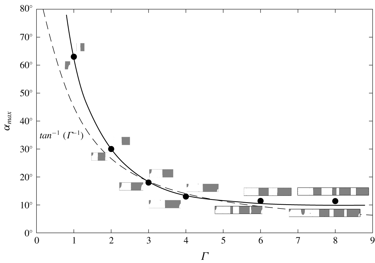
Angle  $\unicode[STIX]{x1D6FC}_{max}$ of the final mode transition in the formation of columnar structures triggered by the frozen wave instability for different container aspect ratios
 $\unicode[STIX]{x1D6E4}=L/(2H)$. This angle is only weakly dependent on forcing, and the values plotted are the average of those found with
 $A\unicode[STIX]{x1D714}=424~\text{mm}~\text{s}^{-1}$ (
 $f=45~\text{Hz}$,
 $A=1.5~\text{mm}$) and
 $565~\text{mm}~\text{s}^{-1}$ (
 $f=60~\text{Hz}$,
 $A=1.5~\text{mm}$). Examples of patterns observed before and after the transition are shown in the insets. The predicted curve based on idealized geometry,
 $\tan ^{-1}(\unicode[STIX]{x1D6E4}^{-1})$, is included (dashed line) for comparison.

In addition to modifying the location of intermediate transitions, the most prominent effect of aspect ratio is on the final angle  $\unicode[STIX]{x1D6FC}_{max}$ where either the two-column state is found or, as described above, the pattern selection process is more complicated but driven by contact conditions and collisions. Figure 11 shows the variation of this maximum angle (filled circles) with container aspect ratio
 $\unicode[STIX]{x1D6E4}$. The observed values are then compared to the formula
 $\unicode[STIX]{x1D6FC}_{max}=\tan ^{-1}(\unicode[STIX]{x1D6E4}^{-1})$ (dashed line) that predicts the corner crossing transition for a perfectly flat unforced interface.
As seen in the figure, the observations lie very close to this curve. The contact angle of  $90^{\circ }$ induces curvature in the initial interface (see figure 8) and delays its contact with the corners. This is most clearly seen for smaller and larger aspect ratios where the measured
 $\unicode[STIX]{x1D6FC}_{max}$ is somewhat above the theoretical prediction. For intermediate aspect ratios, the measured values are closer; the final mode transition in this regime is more influenced by vibrational velocity. In any case, the strong dependence on aspect ratio of both the final mode transition point
 $\unicode[STIX]{x1D6FC}_{max}$ and the final selected wavenumber is clear. For the simulations performed here, the two-column final state is found for
 $\unicode[STIX]{x1D6E4}\lesssim 4$, while four and eight columns are observed for
 $\unicode[STIX]{x1D6E4}=6$ and
 $\unicode[STIX]{x1D6E4}=8$, respectively.
4.2.4 Comparison with experiment
There is some experimental evidence for the importance of the initial interface orientation in microgravity experiments with immiscible liquids, although it is not as clear as in the miscible case of § 2.
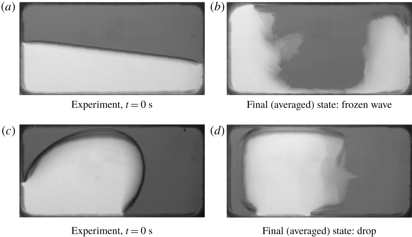
Figure 12 shows initial and final states from two experiments with combination  $\text{I}_{b}$ at identical vibrational velocities. When vibrations are initiated during (the end of) the hypergravity period, with a flat initial interface (figure 12a), the final configuration is an approximately left–right symmetric state consistent with the frozen wave instability (with small angles of initial orientation); the denser FC-40 surrounds the silicone oil (figure 12b). Subharmonic Faraday waves are also excited on the interface in this case, though they are not evident in the figure due to averaging (over approximately two excitation periods).
When vibrations are initiated in microgravity, surface tension (and contact forces) leads to the formation of a drop-like configuration (figure 12c). The applied vibrations act to squeeze and flatten this drop so that, as expected from vibroequilibria theory, large portions of the interface are nearly perpendicular to the forcing. The immiscible simulations presented in § 4.2 do not apply to this case since the initial interface is far from an inclined (linear) profile.
Snapshots showing initial (a,c) and final (b,d) interfacial patterns in experiments with combination  $\text{I}_{b}$ in a parabolic flight. Vibrations at 9 Hz with
 $A=4.4~\text{mm}$ begin during hypergravity (a,b) and during microgravity (c,d). Images showing the final states are averaged over (approximately) two excitation periods.

5 Conclusions
Using careful simulations and available experiments, we demonstrated the importance of the initial interface orientation for pattern selection in miscible and immiscible liquids subjected to horizontal vibrations in microgravity. In a parabolic flight experiment, for example, the level of gravity varies from normal, to about twice that (hypergravity), to about 20 times less (microgravity), with each phase lasting for approximately 22 s. The initial condition for a fluid experiment with a free interface in this environment depends in a critical way on the gravity level that is present when the experiment begins.
Experimental evidence was first presented in the case of miscible liquids, where the evolution of the interface under applied vibrations was traced in four experiments using two distinct pairs of miscible liquids with different initial conditions. A decrease in the wavenumber characterizing the final quasisteady state was observed as the angle of the initial interface with respect to the vibrational axis was increased.
Numerical models based on the solution of the Navier–Stokes equations allowed us to systematically investigate the dependence of interface dynamics on the initial angle. For miscible liquids, this involved an additional equation for the concentration field, while a level-set approach was used to track the interface in the immiscible case. The slow (compared to the forcing) dynamics of the interface motion is reflected in the mean flow, and it was seen how this changes for different initial orientations. With a flat horizontal initial interface, the mean flow during the early transient period is largest near the lateral walls due to the growth and inward spread of the frozen waves, and there is negligible vertical flow in the interior; in the case of immiscible liquids, there is also an approximate left–right symmetry. For oblique initial interfaces, a rotating (vortical) mean flow is generated in the central part of the container that acts to rotate the interface towards a more vertical orientation. The strength of this central mean flow and the associated rotation increases with initial interface angle. It is this rotation of the central portion of the interface that frustrates and interferes with the development of the columnar structures that are characteristic of the frozen wave instability in microgravity.
The dependence of the final quasisteady state on initial inclination was summarized in mode diagrams showing three representative wavenumbers measured along the horizontal midline of the container. Mode transitions to patterns of smaller wavenumber were observed with increasing initial angle. For sufficiently large angles, the selected structure is often one where each fluid primarily occupies one side of the container. The maximum angle characterizing this limit in the immiscible case depends on aspect ratio and is related to the point where the unforced interface crosses the corners of the container. For aspect ratios of approximately 5 and larger, the final state exhibits multiple columns and depends on contact conditions and the dynamics of collisions between the interface and the upper and lower boundaries. Although intermediate mode transitions depend on vibrational velocity, with higher amplitudes favouring more columns, this maximum inclination angle is only weakly dependent on forcing.
Based on the consistency of the numerical simulations for both miscible and immiscible liquids, and on the qualitative agreement with available experimental results, it is clear that the development of interfacial instabilities in microgravity – in particular, the frozen wave instability and potential excitation of secondary Faraday waves – is strongly influenced by the initial position of the interface. This effect must be considered in addition to residual gravity, finite-size effects and other experimental concerns.
Acknowledgements
The work of the Belgian team was supported by the PRODEX programme of the Belgian Federal Science Policy Office. The work of P.S.S. and J.P. was supported by the Ministerio de Economía y Competitividad under project no. ESP2015-70458-P. We also thank the Departamento de Aeronaves y Vehículos Espaciales in the Escuela Técnica Superior de Ingeniería Aeronáutica y del Espacio, Universidad Politécnica de Madrid for supporting the stay of P.S.S. at the Microgravity Research Centre, Université Libre de Bruxelles.
Declaration of interests
The authors report no conflict of interest.