1 Introduction
From the purpose of optimizing artificially fabricated microfluidic systems to controlling blood flows in natural or artificial channels, it is critical to understand the dynamic behaviour of deformable objects in confined geometries (Stone, Stroock & Ajdari Reference Stone, Stroock and Ajdari2004; Stefano & Valentina Reference Stefano and Valentina2010). Morphological evolution of droplets in a continuous immiscible liquid phase in a microconfined flow offers a representative picture that contains many intrinsic attributes of this generic, apparently simple yet elusively complicated physical scenario (Sibillo et al. Reference Sibillo, Pasquariello, Simeone, Cristini and Guido2006). The underlying complexities become significantly magnified when the morphodynamics of a compound droplet, representing the essential features of an encapsulated cellular phase from a biophysical perspective, is considered.
Further complications emerge when a microconfined droplet is subjected to an electric field. The fundamental understanding of the deformation characteristics of such a droplet is of immense interest considering its wide gamut of applications ranging from natural to modern-day microfluidic processes (Teh et al. Reference Teh, Lin, Hung and Lee2008; Mhatre et al. Reference Mhatre, Vivacqua, Ghadiri, Abdullah, Hassanpour, Hewakandamby, Azzopardi and Kermani2015; Li et al. Reference Li, Jun-Yan Suen, Prince, Larin, Klinkova, Thérien-Aubin, Zhu, Yang, Helmy and Lavrentovich2016). While there is the ubiquitous appearance of single-phase droplets in different flow processes, encapsulated droplets (or compound droplets) also have significant attribution in a growing number of emerging applications. Traditionally, these droplets have served the purpose of liquid membranes in selective mass transfer process (Araki & Tsukube Reference Araki and Tsukube1990), in separation of hydrocarbons (Li Reference Li1971), blood oxygenation (Li & Asher Reference Li and Asher1973), mass production foam cell for laser fusion target (Bei et al. Reference Bei, Jones, Tucker-Schwartz and Harding2008; Tucker-Schwartz et al. Reference Tucker-Schwartz, Bei, Garrell and Jones2010), purification of water (Li & Shrier Reference Li, Shrier and Norman1972) and controlled release of drugs (Mataumoto & Kang Reference Mataumoto and Kang1989). In more recent times, compound droplet models have been employed for probing various biophysical processes, for instance, distortion as well as recovery of white blood cells in the presence of incipient flow (Kan et al. Reference Kan, Udaykumar, Shyy and Tran-Son-Tay1998; Tasoglu et al. Reference Tasoglu, Kaynak, Szeri, Demirci and Muradoglu2010). These studies have considered a compound droplet model to mimic the dynamics of a leukocyte, where the core (inner droplet) and shell (outer droplet) denote the cell nucleus and the cytoplasm, respectively. These types of models can be potentially used for developing cell-morphology-based disease detection strategies in in vitro point-of-care diagnostic devices that are fundamentally premised on microfluidic principles.
With the advent of lab-on-a-chip technology, the deployment of electric field as a controlling means towards dictating the morphological evolution of droplets remains inevitable. From the pioneering work of Taylor (Reference Taylor1966), it has been revealed that the interfacial electric stress generated due to the presence of an electric field not only deforms the droplet–carrier fluid interface into a prolate or oblate shape, but also creates a hydrodynamic flow in and around the droplet. For denoting the sense of deformation, Taylor (Reference Taylor1966) has analytically derived a discriminating function
 $(\unicode[STIX]{x1D6FA}_{\text{T}})$
in terms of the parameters
 $S$
,
 $R$
and
 $\unicode[STIX]{x1D706}$
, where
 $S$
,
 $R$
and
 $\unicode[STIX]{x1D706}$
represent the ratios of the permittivity, conductivity and viscosity of the droplet and the surrounding phase, respectively. Later, several studies (Melcher & Taylor Reference Melcher and Taylor1969; Feng & Scott Reference Feng and Scott1996; Feng Reference Feng1999; Lac & Homsy Reference Lac and Homsy2007; Salipante & Vlahovska Reference Salipante and Vlahovska2010; Nganguia & Layton Reference Nganguia and Layton2016; Nganguia et al.
Reference Nganguia, Young, Layton, Lai and Hu2016; Das & Saintillan Reference Das and Saintillan2017a
,Reference Das and Saintillan
b
; Mandal et al.
Reference Mandal, Sinha, Bandopadhyay and Chakraborty2018; Santra, Mandal & Chakraborty Reference Santra, Mandal and Chakraborty2018) have been executed on the electrohydrodynamics (EHD) of single droplets, which explored the various physical facets involved.
Unlike the case of single droplets, significant attention has not been devoted towards the EHD of compound droplets. The earliest study was performed by Gouz & Sadhal (Reference Gouz and Sadhal1989), where they looked into the setting of a compound droplet in the presence of gravity. They investigated the stability of the compound droplet in the presence of an electric field and suggested that a stable equilibrium position of the droplet can be achieved even in the presence of gravitational force. Tsukada et al. (Reference Tsukada, Mayama, Sato and Hozawa1997) have numerically shown that the intensity of the electric field and ratio of core-phase to shell-phase volume have a significant effect on the orientation of fluid circulation as well as the interface deformation. Later on, Ha & Yang (Reference Ha and Yang1999) studied this problem analytically and found out the possibilities for the formation of a double structured vortex. In recent years, Behjatian & Esmaeeli (Reference Behjatian and Esmaeeli2015) have looked into the EHD of compound droplets and shown that there are four types of flow patterns depending on the direction of external fluid flow and the number of vortices. They have also pointed out four possible modes of droplet deformation on the basis of the relative strength of normal electric and hydrodynamic stresses. In a related study, Soni, Juvekar & Naik (Reference Soni, Juvekar and Naik2013) have shown that the presence of an inner droplet alters the deformation of the outer droplet.
Though the general features of steady-state and transient EHD of droplets have been well studied (Mandal, Chaudhury & Chakraborty Reference Mandal, Chaudhury and Chakraborty2014; Mandal et al. Reference Mandal, Sinha, Bandopadhyay and Chakraborty2018; Santra et al. Reference Santra, Mandal and Chakraborty2018), the shape evolution of a compound liquid droplet in a confined fluidic environment is yet to be reported, despite its potential relevance in a vast body of emerging applications, including the biological perspectives outlined earlier. In two relevant studies, Esmaeeli & Behjatian (Reference Esmaeeli and Behjatian2012) and Behjatian & Esmaeeli (Reference Behjatian and Esmaeeli2013) have reported the EHD of a single liquid column (and a single droplet) in a cylindrical (and spherical) confined domain. However, their studies, as well as the recent investigations of Santra et al. (Reference Santra, Mandal and Chakraborty2018), were limited only to simple droplets, restricting their applicability towards explaining the functionalities of encapsulated cellular systems in confined fluidic passages. As a consequence, in spite of its vast scientific and technological relevance, the present state of understanding of confinement-induced dynamical evolution of biologically relevant entities under an electric field remains rather inadequate. This deficit stems from the complexities in understanding the combined confluences of the extent of confinement and local electric field on the morphological evolution of compound biomimetic droplets.
Here, we report non-intuitive findings on the shape evolutions of compound liquid droplets in a microconfined fluidic environment, under the critical influence of an incipient electric field. We capture the intricate coupling between local electric field and confinement-induced hydrodynamic interactions towards dictating the underlying morphological evolution. In particular, we probe the effect of channel confinement on the steady-state morphology of a compound droplet, the transient evolution of its configuration as well as the motion of an eccentric inner droplet with respect to the outer. Our findings imply that the deformation of either of the interfaces can change depending on the degree of confinement of the system similar to that of a single droplet. However, the interplay of the electric field with the confinement-induced hydrodynamics is shown to alter the underlying shape evolution non-trivially, in a manner that is distinct from the morphodynamics of single droplets. Furthermore, we show that an eccentrically placed inner droplet undergoes linear translational motion in a highly confined domain, in sharp contrast to the to-and-fro motion in a weakly confined domain. In an attempt to unveil the essential aspects of some of the fundamental physical features involved, we also present an asymptotic analysis considering higher-order terms for the unconfined scenario, and establish the numerical results from the perspective of that as a limiting case of a weakly confined domain.
2 Problem formulation
2.1 Compound droplet in unbounded domain
2.1.1 System description
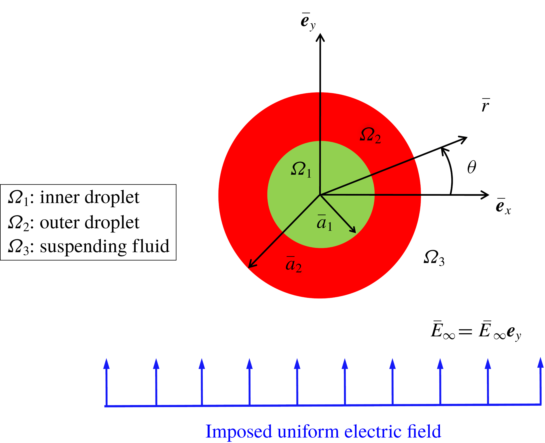
Figure 1 shows the schematic of the physical system, where a neutrally buoyant compound droplet is suspended in another medium under the influence of a uniform electric field.
Schematic illustration of the problem set-up, where a Newtonian neutrally buoyant compound droplet is suspended in another Newtonian liquid medium under a transverse uniform electric field.

All the phases are Newtonian, immiscible and incompressible in nature, with the radius of the outer and the inner undeformed interfaces being
 $a_{1}$
and
 $a_{2}$
, respectively. Properties such as viscosity, electrical permittivity, electrical conductivity and surface tension are represented by
 $\unicode[STIX]{x1D707}$
,
 $\unicode[STIX]{x1D700}$
,
 $\unicode[STIX]{x1D70E}$
and
 $\unicode[STIX]{x1D6FE}$
, respectively. Subscripts 1, 2 and 3 denote the inner phase (inner droplet, fluid 1), outer phase (outer droplet, fluid 2) and carrier fluid phase (fluid 3), respectively, whereas the double subscripts 12 and 23 represent the inner and outer interfaces, respectively. The present analysis utilizes cylindrical polar coordinates
 $(\overline{r},\unicode[STIX]{x1D703})$
attached to the droplet centroid.
2.1.2 Assumptions
The assumptions taken into consideration for simplifying the mathematical model are as follows. (i) The viscous force and pressure force regulate the flow problem as compared to fluid inertia. This implies that the value of the Reynolds number
 $(Re=\unicode[STIX]{x1D70C}\unicode[STIX]{x1D700}_{3}\overline{E}_{\infty }^{2}\overline{a}_{2}^{2}/\unicode[STIX]{x1D707}_{3}^{2})$
is negligible
 $(Re\sim O(10^{-4}))$
. (ii) The densities of the fluid phases are the same, rendering the system neutrally buoyant
 $(\unicode[STIX]{x1D70C}_{r}=\unicode[STIX]{x1D70C}_{1}/\unicode[STIX]{x1D70C}_{2}=\unicode[STIX]{x1D70C}_{2}/\unicode[STIX]{x1D70C}_{3}=1)$
. (iii) The effect of electric charge convection has been neglected which means the magnitude of the electric Reynolds number
 $(Re_{E}=\unicode[STIX]{x1D700}_{3}^{2}\overline{E}_{\infty }^{2}/\unicode[STIX]{x1D707}_{3}\unicode[STIX]{x1D70E}_{3})$
is much less. A typical example of such a type of microfluidic system is presented as follows. A compound droplet having inner radius 2 mm and outer radius 4 mm is suspended in another fluid medium under a transverse electric field. The strength of the electric field is
 $1\times 10^{5}~\text{V}~\text{m}^{-1}$
. The inner droplet phase and the carrier phase are silicone oil (having
 $\unicode[STIX]{x1D700}=2.44\times 10^{-11}~\text{F}~\text{m}^{-1}$
,
 $\unicode[STIX]{x1D70E}=3.33\times 10^{-11}~\text{S}~\text{m}^{-1}$
,
 $\unicode[STIX]{x1D707}=12~\text{Pa}~\text{s}$
and
 $\unicode[STIX]{x1D70C}=980~\text{kg}~\text{m}^{-3}$
) and the outer droplet phase is oxidized castor oil (having
 $\unicode[STIX]{x1D700}=10^{-9}~\text{F}~\text{m}^{-1}$
,
 $\unicode[STIX]{x1D70E}=5.57\times 10^{-11}~\text{S}~\text{m}^{-1}$
,
 $\unicode[STIX]{x1D707}=6.5~\text{Pa}~\text{s}$
and
 $\unicode[STIX]{x1D70C}=980~\text{kg}~\text{m}^{-3}$
). The interfacial tension between the fluid phase is
 $5.5~\text{mN}~\text{m}^{-1}$
. The properties of the interacting fluid have been taken from the experimental study of Torza, Cox & Mason (Reference Torza, Cox and Mason1971). The calculated values of the non-dimensional parameters are
 $Re_{E}\sim O(10^{-2})$
,
 $Re\sim O(10^{-4})$
and
 $\unicode[STIX]{x1D70C}_{r}=1$
.
2.1.3 Governing equations and boundary conditions
In the current study, we have taken the leaky dielectric model into consideration. In the leaky dielectric model, the free charges are assumed to move instantaneously to the interface. Hence, the bulk remains electrically neutral (Saville Reference Saville1997). Thus, the equations governing the electric field and the flow field are decoupled from each other and the problem is reduced to an electrostatic problem. Furthermore, the applied electric field is also irrotational and it is expressed as
 $\overline{\boldsymbol{E}}=-\overline{\unicode[STIX]{x1D735}}\overline{\unicode[STIX]{x1D711}}$
(Baygents, Rivette & Stone Reference Baygents, Rivette and Stone1998; Reddy & Esmaeeli Reference Reddy and Esmaeeli2009; Lanauze, Walker & Khair Reference Lanauze, Walker and Khair2015). The dimensional quantities in the present analysis are denoted by the overbar. The non-dimensional set of governing equations and boundary conditions are derived with the help of the following non-dimensional scheme: length
 ${\sim}\overline{a}_{2}$
, velocity
 $(\overline{u}_{c})\sim \unicode[STIX]{x1D700}_{3}\overline{E}_{\infty }^{2}\overline{a}_{2}/\unicode[STIX]{x1D707}_{3}$
, time
 ${\sim}\overline{a}_{2}/\overline{u}_{c}$
, viscous stress
 ${\sim}\unicode[STIX]{x1D707}_{3}\overline{u}_{c}/\overline{a}_{2}$
and
 $q_{s}\sim \unicode[STIX]{x1D700}_{3}\overline{E}_{\infty }$
. The velocity scale is obtained by balancing the electric stress and hydrodynamic stress at the interface of the droplet; and
 $\overline{E}_{\infty }$
and
 $\unicode[STIX]{x1D700}_{3}\overline{E}_{\infty }^{2}$
have been used as characteristic scales for the applied electric field and electric stress, respectively.
After applying the non-dimensionalization scheme, the governing electric potential distribution (
 $\unicode[STIX]{x1D711}$
) for the
 $i$
th (
 $i=1,2,3$
) fluid reads
 $$\begin{eqnarray}\unicode[STIX]{x1D6FB}^{2}\unicode[STIX]{x1D711}_{i}=0.\end{eqnarray}$$
The essential boundary conditions take the form
 $$\begin{eqnarray}\left.\begin{array}{@{}l@{}}\displaystyle (\text{i})~\unicode[STIX]{x1D711}_{1}\text{ is finite},\quad \text{at }r\rightarrow 0,\\ \displaystyle (\text{ii})~\unicode[STIX]{x1D711}_{3}\rightarrow -r\sin (\unicode[STIX]{x1D703}),\quad \text{at }r\rightarrow \infty ,\\ \displaystyle (\text{iii})~[\unicode[STIX]{x1D711}_{i}]_{\unicode[STIX]{x1D6F1}_{ij}}=[\unicode[STIX]{x1D711}_{j}]_{\unicode[STIX]{x1D6F1}_{ij}},\quad \text{at }r=r_{\unicode[STIX]{x1D6F1}_{ij}}(\unicode[STIX]{x1D703},t),\\ \displaystyle (\text{iv})~Sa\left[\frac{\unicode[STIX]{x2202}q_{s}}{\unicode[STIX]{x2202}t}\right]_{\unicode[STIX]{x1D6F1}_{ij}}+Re_{E}[\unicode[STIX]{x1D735}_{s}\boldsymbol{\cdot }(\boldsymbol{u}_{s}q_{s})]_{\unicode[STIX]{x1D6F1}_{ij}}\\ =[\unicode[STIX]{x1D70E}_{j}\unicode[STIX]{x1D735}\unicode[STIX]{x1D711}_{j}\boldsymbol{\cdot }\boldsymbol{n}_{ij}]_{\unicode[STIX]{x1D6F1}_{ij}}-[\unicode[STIX]{x1D70E}_{i}\unicode[STIX]{x1D735}\unicode[STIX]{x1D711}_{i}\boldsymbol{\cdot }\boldsymbol{n}_{ij}]_{\unicode[STIX]{x1D6F1}_{ij}},\quad \text{at }r=r_{\unicode[STIX]{x1D6F1}_{ij}}(\unicode[STIX]{x1D703},t),\end{array}\right\}\end{eqnarray}$$
where the normal unit vector in the outward direction at the interface
 $\unicode[STIX]{x1D6F1}_{ij}$
is denoted by
 $\boldsymbol{n}_{ij}$
(Mandal, Ghosh & Chakraborty Reference Mandal, Ghosh and Chakraborty2016b
). We have employed the general notation
 $[~]_{\unicode[STIX]{x1D6F1}_{ij}}$
to denote any quantity at the interface
 $\unicode[STIX]{x1D6F1}_{ij}$
. Here
 $\unicode[STIX]{x1D735}_{s}$
is the surface gradient operator expressed as
 $\unicode[STIX]{x1D735}_{s}=\unicode[STIX]{x1D735}_{ij}-\boldsymbol{n}_{ij}(\boldsymbol{n}_{ij}\boldsymbol{\cdot }\unicode[STIX]{x1D735}_{ij})$
,
 $\boldsymbol{u}_{\boldsymbol{s}}$
is the interfacial velocity and
 $q_{s}$
is the surface charge density that is developed due to the mismatch between material properties and expressed as
 $q_{s}=(\unicode[STIX]{x1D700}_{i}\unicode[STIX]{x1D735}\unicode[STIX]{x1D711}_{i}-\unicode[STIX]{x1D700}_{j}\unicode[STIX]{x1D735}\unicode[STIX]{x1D711}_{j})\boldsymbol{\cdot }\boldsymbol{n}_{ij}$
. It is worth mentioning that the present physical system is two-dimensional in nature. The non-dimensional numbers present in (2.2) are the electric Reynolds number,
 $Re_{E}=\unicode[STIX]{x1D700}_{3}^{2}\overline{E}_{\infty }^{2}/\unicode[STIX]{x1D707}_{3}\unicode[STIX]{x1D70E}_{3}$
, and the Saville number,
 $Sa=Re_{E}/Ca_{E}$
, where
 $Ca_{E}$
symbolizes the electric capillary number expressed as
 $Ca_{E}=\unicode[STIX]{x1D700}_{3}\overline{E}_{\infty }^{2}\overline{a}_{2}/\unicode[STIX]{x1D6FE}_{23}$
. At a low value of
 $Re_{E}~({\sim}O(10^{-2}))$
, the boundary condition (iv) of (2.2) is simplified to the following form:
 $$\begin{eqnarray}[\unicode[STIX]{x1D70E}_{j}\unicode[STIX]{x1D735}\unicode[STIX]{x1D711}_{j}\boldsymbol{\cdot }\boldsymbol{n}_{ij}]_{\unicode[STIX]{x1D6F1}_{ij}}-[\unicode[STIX]{x1D70E}_{i}\unicode[STIX]{x1D735}\unicode[STIX]{x1D711}_{i}\boldsymbol{\cdot }\boldsymbol{n}_{ij}]_{\unicode[STIX]{x1D6F1}_{ij}}=0.\end{eqnarray}$$
The governing continuity and Navier–Stokes equations for
 $i$
th fluid (
 $i=1,2,3$
) are presented in the following non-dimensional form:
 $$\begin{eqnarray}\unicode[STIX]{x1D735}\boldsymbol{\cdot }\boldsymbol{u}_{i}=0,\quad Re\left(\frac{\unicode[STIX]{x2202}\boldsymbol{u}_{i}}{\unicode[STIX]{x2202}t}+\unicode[STIX]{x1D735}\boldsymbol{\cdot }(\boldsymbol{u}_{i}\boldsymbol{u}_{i})\right)=-\unicode[STIX]{x1D735}p_{i}+\unicode[STIX]{x1D735}\boldsymbol{\cdot }[\unicode[STIX]{x1D706}\{\unicode[STIX]{x1D735}\boldsymbol{u}_{i}+(\unicode[STIX]{x1D735}\boldsymbol{u}_{i})^{\text{T}}\}].\end{eqnarray}$$
Under the paradigm of creeping flow condition
 $(Re=0)$
, the fluid flow problem is regulated by the Stokes equation and incompressibility condition as follows:
 $$\begin{eqnarray}\left.\begin{array}{@{}c@{}}\unicode[STIX]{x1D735}p_{1}=\unicode[STIX]{x1D706}_{12}\unicode[STIX]{x1D6FB}^{2}u_{1},\quad \unicode[STIX]{x1D735}\boldsymbol{\cdot }u_{1}=0,\\ \unicode[STIX]{x1D735}p_{2}=\unicode[STIX]{x1D706}_{23}\unicode[STIX]{x1D6FB}^{2}u_{2},\quad \unicode[STIX]{x1D735}\boldsymbol{\cdot }u_{2}=0,\\ \unicode[STIX]{x1D735}p_{3}=\unicode[STIX]{x1D6FB}^{2}u_{3},\quad \unicode[STIX]{x1D735}\boldsymbol{\cdot }u_{3}=0.\end{array}\right\}\end{eqnarray}$$
The boundary conditions are expressed in the following form:
 $$\begin{eqnarray}\left.\begin{array}{@{}l@{}}\displaystyle (\text{i})~[\boldsymbol{u}_{i}]_{\unicode[STIX]{x1D6F1}_{ij}}=[\boldsymbol{u}_{j}]_{\unicode[STIX]{x1D6F1}_{ij}},\quad \text{at }r=r_{\unicode[STIX]{x1D6F1}_{ij}}(\unicode[STIX]{x1D703},t),\\ \displaystyle (\text{ii})~[\boldsymbol{u}_{i}\boldsymbol{\cdot }\boldsymbol{n}_{ij}]_{\unicode[STIX]{x1D6F1}_{ij}}=[\boldsymbol{u}_{j}\boldsymbol{\cdot }\boldsymbol{n}_{ij}]_{\unicode[STIX]{x1D6F1}_{ij}}=\frac{\text{d}\boldsymbol{r}_{\unicode[STIX]{x1D6F1}_{ij}}}{\text{d}t},\quad \text{at }r=r_{\unicode[STIX]{x1D6F1}_{ij}}(\unicode[STIX]{x1D703},t),\\ \displaystyle (\text{iii})~[(\unicode[STIX]{x1D749}_{j}^{H}+\unicode[STIX]{x1D749}_{j}^{E})\boldsymbol{\cdot }\boldsymbol{n}_{ij}]_{\unicode[STIX]{x1D6F1}_{ij}}-[(\unicode[STIX]{x1D749}_{i}^{H}+\unicode[STIX]{x1D749}_{i}^{E})\boldsymbol{\cdot }\boldsymbol{n}_{ij}]_{\unicode[STIX]{x1D6F1}_{ij}}=\frac{1}{Ca_{E}}(\unicode[STIX]{x1D735}\boldsymbol{\cdot }\boldsymbol{n}_{ij})\boldsymbol{n}_{ij},\quad \text{at }r=r_{\unicode[STIX]{x1D6F1}_{ij}}(\unicode[STIX]{x1D703},t).\end{array}\right\}\end{eqnarray}$$
In (2.6), the electric and hydrodynamic stress tensors are denoted by
 $\unicode[STIX]{x1D749}^{E}$
and
 $\unicode[STIX]{x1D749}^{H}$
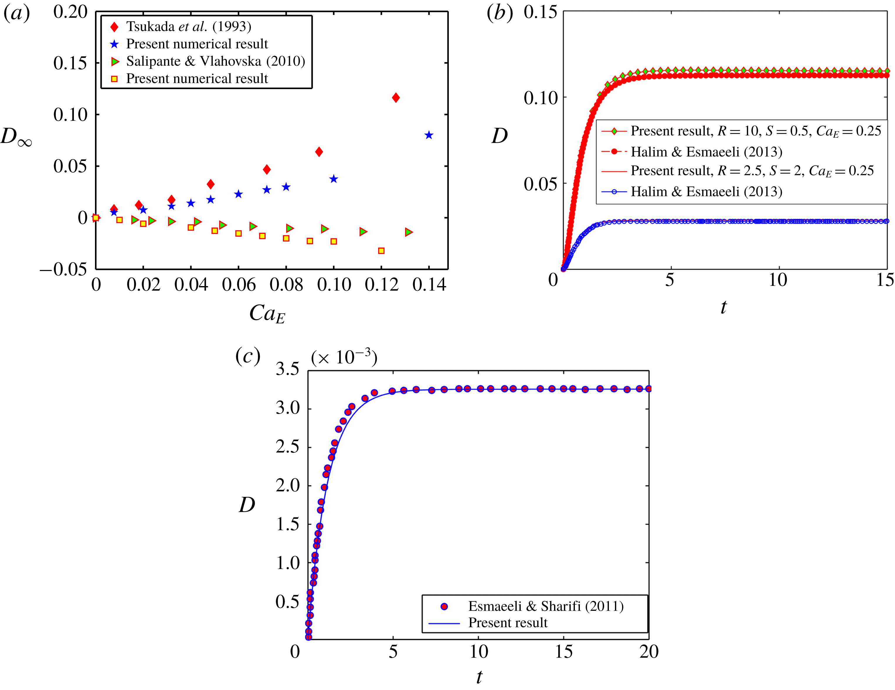
, respectively. All the dimensionless parameters are written in table 1. The details of the analytical solution are given in § 1 of the supplementary material, which is available at https://doi.org/10.1017/jfm.2019.810.
Some important dimensionless parameters
 $[i,j\in (1,3)]$
.

2.2 Compound droplet in confined domain
Before discussing the details of the problem formulation for a compound droplet in a highly confined domain, one must acknowledge that the present mathematical problem is nonlinear and coupled, which restricts us to obtain its exact analytical solution for any arbitrary value of the non-dimensional parameters in an unbounded domain. Further complexity arises when the domain confinement is taken into consideration. Keeping this information in mind, we have taken the help of numerical simulation for examining the essential physics of the EHD of a compound droplet in a highly confined channel. Towards performing a numerical simulation of the present problem, we have employed the diffuse-interface-based phase field method for tracking the fluid–fluid interface (Jacqmin Reference Jacqmin1999; Badalassi, Ceniceros & Banerjee Reference Badalassi, Ceniceros and Banerjee2003; Santra, Mandal & Chakraborty Reference Santra, Mandal and Chakraborty2019a
). For a weakly confined system
 $(Wc\leqslant 0.2)$
, our theoretical prediction agrees closely with the numerical outcome. The details of the numerical analysis are provided in the following section.
2.2.1 Numerical set-up
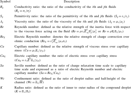
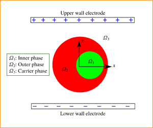
We have represented the schematic of the present computational domain in figure 2, where a Newtonian double-emulsion droplet is suspended in another Newtonian medium in the presence of a transverse electric field. The inner droplet is taken to be located eccentrically with respect to the outer droplet in order to take into account the effect of eccentricity in the numerical analysis.
Schematic of the problem set-up displaying a compound droplet placed in between two parallel-plate electrodes. The radius of the core (inner droplet) and shell (outer droplet) are
 $\overline{a}_{1}$
and
 $\overline{a}_{2}$
, respectively.

The eccentricity is
 $\overline{e}$
(refer to figure 2). The separating distance between the two walls is
 $2\overline{H}$
and the electric field strength is denoted by
 $\overline{E}_{\infty }$
. Thus the electric potentials of the top wall and bottom wall electrodes are taken as
 $\overline{H}\overline{E}_{\infty }$
and
 $-\overline{H}\overline{E}_{\infty }$
, respectively. The radii of the outer and the inner undeformed interfaces are
 $\overline{a}_{1}$
and
 $\overline{a}_{2}$
, respectively.
2.2.2 Governing equation for electric potential coupled with phase field formalism
For the present analysis, we have taken two systems into consideration: (i) leaky dielectric system (LD–LD–LD) and (ii) perfect dielectric system (PD–PD–PD).
For the leaky dielectric system, the conservation of ionic species at the interface can be expressed in dimensional form as (Saville Reference Saville1997)
 $$\begin{eqnarray}\frac{\unicode[STIX]{x2202}n_{s}^{k}}{\unicode[STIX]{x2202}\overline{t}}+\overline{\boldsymbol{u}}\boldsymbol{\cdot }\overline{\unicode[STIX]{x1D735}}_{s}n_{s}^{k}=n_{s}^{k}\boldsymbol{n}\boldsymbol{\cdot }(\boldsymbol{n}\boldsymbol{\cdot }\overline{\unicode[STIX]{x1D735}})\overline{\boldsymbol{u}}+\Vert \unicode[STIX]{x1D714}^{k}e_{p}z^{k}n^{k}\overline{\unicode[STIX]{x1D735}}\unicode[STIX]{x1D711}+\unicode[STIX]{x1D714}^{k}k_{B}T\overline{\unicode[STIX]{x1D735}}n^{k}\Vert ,\end{eqnarray}$$
where
 $\overline{\unicode[STIX]{x1D735}}_{s}$
symbolizes the surface divergence,
 $n_{s}^{k}$
denotes the surface concentration of ionic species,
 $\unicode[STIX]{x1D714}^{k}$
represents the mobility of the
 $k$
th species,
 $e_{p}$
is the charge of the proton,
 $k_{B}$
is the Boltzmann constant,
 $n^{k}$
symbolizes the ionic concentration of the
 $k$
th species,
 $z^{k}$
denotes the valence of the
 $k$
th species and
 $T$
is the absolute temperature. Now, if the surface charge density is
 $\overline{q}_{s}$
, equation (2.7) can be interpreted as (Saville Reference Saville1997)
 $$\begin{eqnarray}\displaystyle \frac{\unicode[STIX]{x2202}\overline{q}_{s}}{\unicode[STIX]{x2202}\overline{t}}+\overline{\boldsymbol{u}}\boldsymbol{\cdot }\overline{\unicode[STIX]{x1D735}}_{s}\overline{q}_{s} & = & \displaystyle \overline{q}_{s}\boldsymbol{n}\boldsymbol{\cdot }(\boldsymbol{n}\boldsymbol{\cdot }\overline{\unicode[STIX]{x1D735}})\overline{\boldsymbol{u}}+\Vert -e_{p}^{2}(\unicode[STIX]{x1D714}^{2}n^{2}+\unicode[STIX]{x1D714}^{3}n^{3})\overline{\boldsymbol{E}}\Vert \boldsymbol{\cdot }\boldsymbol{n}\nonumber\\ \displaystyle & & \displaystyle +\,\Vert k_{b}T\overline{\unicode[STIX]{x1D735}}(e_{p}\unicode[STIX]{x1D714}^{2}n^{2}-e_{p}\unicode[STIX]{x1D714}^{3}n^{3})\Vert \boldsymbol{\cdot }\boldsymbol{n}.\end{eqnarray}$$
Under the condition of negligible charge diffusion, the equation reduces to (Saville Reference Saville1997)
 $$\begin{eqnarray}\frac{\unicode[STIX]{x2202}\overline{q}_{s}}{\unicode[STIX]{x2202}\overline{t}}+\overline{\boldsymbol{u}}\boldsymbol{\cdot }\overline{\unicode[STIX]{x1D735}}_{s}\overline{q}_{s}=\overline{q}_{s}\boldsymbol{n}\boldsymbol{\cdot }(\boldsymbol{n}\boldsymbol{\cdot }\overline{\unicode[STIX]{x1D735}})\overline{\boldsymbol{u}}+\Vert (\overline{\unicode[STIX]{x1D70E}}\overline{\unicode[STIX]{x1D735}}\unicode[STIX]{x1D711})\Vert .\end{eqnarray}$$
Here
 $\overline{q}_{s}$
can be computed as
 $\overline{\unicode[STIX]{x1D735}}\boldsymbol{\cdot }(\overline{\unicode[STIX]{x1D700}}\overline{\unicode[STIX]{x1D735}}\unicode[STIX]{x1D711})=-\overline{q}_{s}$
. In a leaky dielectric model, the charge relaxation time scale is much smaller compared to the charge convection time scale. Hence, the charges present at the bulk fluid will move instantaneously to the fluid–fluid interface and the bulk flow remains charge-free. For that reason, the charge conservation equations in the bulk fluid and in the fluid–fluid interface (2.8) become identical. Thus, the volumetric charge conservation equation can be read as (Mandal, Bandopadhyay & Chakraborty Reference Mandal, Bandopadhyay and Chakraborty2016a
)
 $$\begin{eqnarray}\frac{\unicode[STIX]{x2202}\overline{q}_{e}}{\unicode[STIX]{x2202}\overline{t}}+\overline{\unicode[STIX]{x1D735}}\boldsymbol{\cdot }(\overline{q}_{e}\overline{\boldsymbol{u}})=\overline{\unicode[STIX]{x1D735}}\boldsymbol{\cdot }\left[\mathop{\sum }_{k}\unicode[STIX]{x1D714}^{k}e_{p}^{2}z^{k}n^{k}\overline{\unicode[STIX]{x1D735}}\unicode[STIX]{x1D719}+\unicode[STIX]{x1D714}^{k}k_{B}T\overline{\unicode[STIX]{x1D735}}q_{e}\right],\quad k=1,2,\ldots ,N.\end{eqnarray}$$
Under the condition of negligible charge diffusion, the volumetric charge conservation equation reduces to (Saville Reference Saville1997; López-Herrera, Popinet & Herrada Reference López-Herrera, Popinet and Herrada2011; Mandal et al. Reference Mandal, Bandopadhyay and Chakraborty2016a , Reference Mandal, Sinha, Bandopadhyay and Chakraborty2018; Das & Saintillan Reference Das and Saintillan2017a )
 $$\begin{eqnarray}\frac{\unicode[STIX]{x2202}\overline{q}_{e}}{\unicode[STIX]{x2202}\overline{t}}+\overline{\unicode[STIX]{x1D735}}\boldsymbol{\cdot }(\overline{q}_{e}\overline{\boldsymbol{u}})=\overline{\unicode[STIX]{x1D735}}\boldsymbol{\cdot }(\unicode[STIX]{x1D70E}\overline{\unicode[STIX]{x1D735}}\unicode[STIX]{x1D711}),\quad \text{where }\overline{q}_{e}=-\overline{\unicode[STIX]{x1D735}}\boldsymbol{\cdot }(\overline{\unicode[STIX]{x1D700}}\overline{\unicode[STIX]{x1D735}}\overline{\unicode[STIX]{x1D711}}).\end{eqnarray}$$
In non-dimensional form, equation (2.11) is read as
 $$\begin{eqnarray}Re_{E}\left(\frac{\unicode[STIX]{x2202}q_{e}}{\unicode[STIX]{x2202}\overline{t}}+\unicode[STIX]{x1D735}\boldsymbol{\cdot }(q_{e}\boldsymbol{u})\right)=\unicode[STIX]{x1D735}\boldsymbol{\cdot }(\unicode[STIX]{x1D70E}\unicode[STIX]{x1D735}\unicode[STIX]{x1D711}).\end{eqnarray}$$
For very small values of
 $Re_{E}$
(refer to § 3 of the supplementary material for details), equation (2.12) is expressed as (Baygents et al.
Reference Baygents, Rivette and Stone1998; Lac & Homsy Reference Lac and Homsy2007; Mahlmann & Papageorgiou Reference Mahlmann and Papageorgiou2009)
 $$\begin{eqnarray}\unicode[STIX]{x1D735}\boldsymbol{\cdot }(\unicode[STIX]{x1D70E}\unicode[STIX]{x1D735}\unicode[STIX]{x1D711})=0.\end{eqnarray}$$
In a similar way, for the perfect dielectric system, the distribution of electric potential is obtained by solving the governing equation, which can be expressed as
 $$\begin{eqnarray}\unicode[STIX]{x1D735}\boldsymbol{\cdot }(\unicode[STIX]{x1D700}\unicode[STIX]{x1D735}\unicode[STIX]{x1D711})=0.\end{eqnarray}$$
In (2.13) and (2.14),
 $\unicode[STIX]{x1D70E}$
and
 $\unicode[STIX]{x1D700}$
for a three-phase system
 $[i,j\in (1,3)]$
are represented in the following form (Lin, Skjetne & Carlson Reference Lin, Skjetne and Carlson2012; Santra et al.
Reference Santra, Mandal and Chakraborty2018)
 $$\begin{eqnarray}\unicode[STIX]{x1D70E}=\frac{(1+\unicode[STIX]{x1D713})}{2}R_{ij}+\frac{(1-\unicode[STIX]{x1D713})}{2}\quad \text{and}\quad \unicode[STIX]{x1D700}=\frac{(1+\unicode[STIX]{x1D713})}{2}S_{ij}+\frac{(1-\unicode[STIX]{x1D713})}{2},\end{eqnarray}$$
where
 $\unicode[STIX]{x1D713}$
is the phase field parameter, which takes certain values for denoting different fluid phase. For fluid 1 (inner droplet) and fluid 3 (suspending fluid), we have taken
 $\unicode[STIX]{x1D713}(\boldsymbol{x},t)=-1$
, whereas
 $\unicode[STIX]{x1D713}(\boldsymbol{x},t)=1$
is taken for fluid 2 (outer droplet). At the interface, the value of
 $\unicode[STIX]{x1D713}(\boldsymbol{x},t)$
varies from
 $-1$
to
 $+1$
rapidly. The order parameter
 $\unicode[STIX]{x1D713}(\boldsymbol{x},t)$
is regulated by the Cahn–Hilliard equation in the following form (Santra et al.
Reference Santra, Sen, Das and Chakraborty2019b
)
 $$\begin{eqnarray}\frac{\unicode[STIX]{x2202}\unicode[STIX]{x1D713}}{\unicode[STIX]{x2202}\overline{t}}+\boldsymbol{u}\boldsymbol{\cdot }\unicode[STIX]{x1D735}\unicode[STIX]{x1D713}=\frac{1}{Pe}\unicode[STIX]{x1D6FB}^{2}G.\end{eqnarray}$$
The non-dimensional quantities in (2.16) are
 $G=(\unicode[STIX]{x1D713}^{3}-\unicode[STIX]{x1D713})/Cn-Cn\unicode[STIX]{x1D6FB}^{2}\unicode[STIX]{x1D713}$
, which is the non-dimensional chemical potential, where
 $Cn$
is the Cahn number, which controls the interface thickness. Another important non-dimensional parameter is the Péclet number denoted as
 $Pe={\overline{a}_{2}}^{2}\overline{u}_{c}/\overline{M}_{\unicode[STIX]{x1D713}}\unicode[STIX]{x1D6FE}$
(the ratio of convective and diffusive transport of the phase field order parameter). In the expression of
 $Pe$
,
 $\overline{M}_{\unicode[STIX]{x1D713}}$
symbolizes the interface mobility factor.
2.2.3 Coupling between phase field and electrohydrodynamics
Under the paradigm of the phase field method, the pressure and the velocity field can be obtained by solving the continuity and Cahn–Hilliard Navier–Stokes equation. The latter equation couples the phase field formalism with the EHD. The continuity and Cahn–Hilliard Navier–Stokes equation are expressed in the following non-dimensional form:
 $$\begin{eqnarray}\unicode[STIX]{x1D735}\boldsymbol{\cdot }\boldsymbol{u}=0,\quad Re\left(\frac{\unicode[STIX]{x2202}\boldsymbol{u}}{\unicode[STIX]{x2202}t}+\unicode[STIX]{x1D735}\boldsymbol{\cdot }(\boldsymbol{u}\boldsymbol{u})\right)=-\unicode[STIX]{x1D735}p+\unicode[STIX]{x1D735}\boldsymbol{\cdot }[\unicode[STIX]{x1D707}\{\unicode[STIX]{x1D735}\boldsymbol{u}+(\unicode[STIX]{x1D735}\boldsymbol{u})^{\text{T}}\}]+\frac{1}{Ca_{E}}G\unicode[STIX]{x1D735}\unicode[STIX]{x1D713}+\boldsymbol{F}^{E}.\end{eqnarray}$$
In (2.17),
 $\boldsymbol{F}^{E}=\unicode[STIX]{x1D735}\boldsymbol{\cdot }(\unicode[STIX]{x1D700}\unicode[STIX]{x1D735}\unicode[STIX]{x1D711})\unicode[STIX]{x1D735}\unicode[STIX]{x1D711}-|\unicode[STIX]{x1D735}\unicode[STIX]{x1D711}|^{2}\unicode[STIX]{x1D735}\unicode[STIX]{x1D700}/2$
represents the volumetric electric force that is responsible for any interfacial deformation. The first term in the expression for
 $F^{E}$
represents the electrophoretic force whereas the second term denotes the dielectrophoretic force. One must acknowledge that, for a perfect dielectric system, the electrophoretic force is not present due to the absence of free charges. It is also worth noting from (2.17) that the volumetric electric force is present in the governing Navier–Stokes equation in the diffuse interface framework unlike the sharp interface limit. The term
 $G\unicode[STIX]{x1D735}\unicode[STIX]{x1D713}$
represents the phase-field-dependent interfacial tension force. Under the phase field framework,
 $\unicode[STIX]{x1D707}$
and
 $\unicode[STIX]{x1D70C}$
are expressed in the following forms:
 $$\begin{eqnarray}\unicode[STIX]{x1D70C}=\frac{(1+\unicode[STIX]{x1D713})}{2}\unicode[STIX]{x1D70C}_{r}+\frac{(1-\unicode[STIX]{x1D713})}{2},\quad \unicode[STIX]{x1D707}=\frac{(1+\unicode[STIX]{x1D713})}{2}\unicode[STIX]{x1D706}_{ij}+\frac{(1-\unicode[STIX]{x1D713})}{2}.\end{eqnarray}$$
One must acknowledge that the pressure field, velocity field and the phase field parameter are periodic in the horizontal direction and expressed in the following forms:
 $$\begin{eqnarray}\left.\begin{array}{@{}l@{}}(\text{i})~\boldsymbol{u}(\boldsymbol{x})=\boldsymbol{u}(\boldsymbol{x}+L),\\ (\text{ii})~p(\boldsymbol{x})=p(\boldsymbol{x}+L),\\ (\text{iii})~\unicode[STIX]{x1D713}(\boldsymbol{x})=\unicode[STIX]{x1D713}(\boldsymbol{x}+L).\end{array}\right\}\end{eqnarray}$$
3 Results and discussion
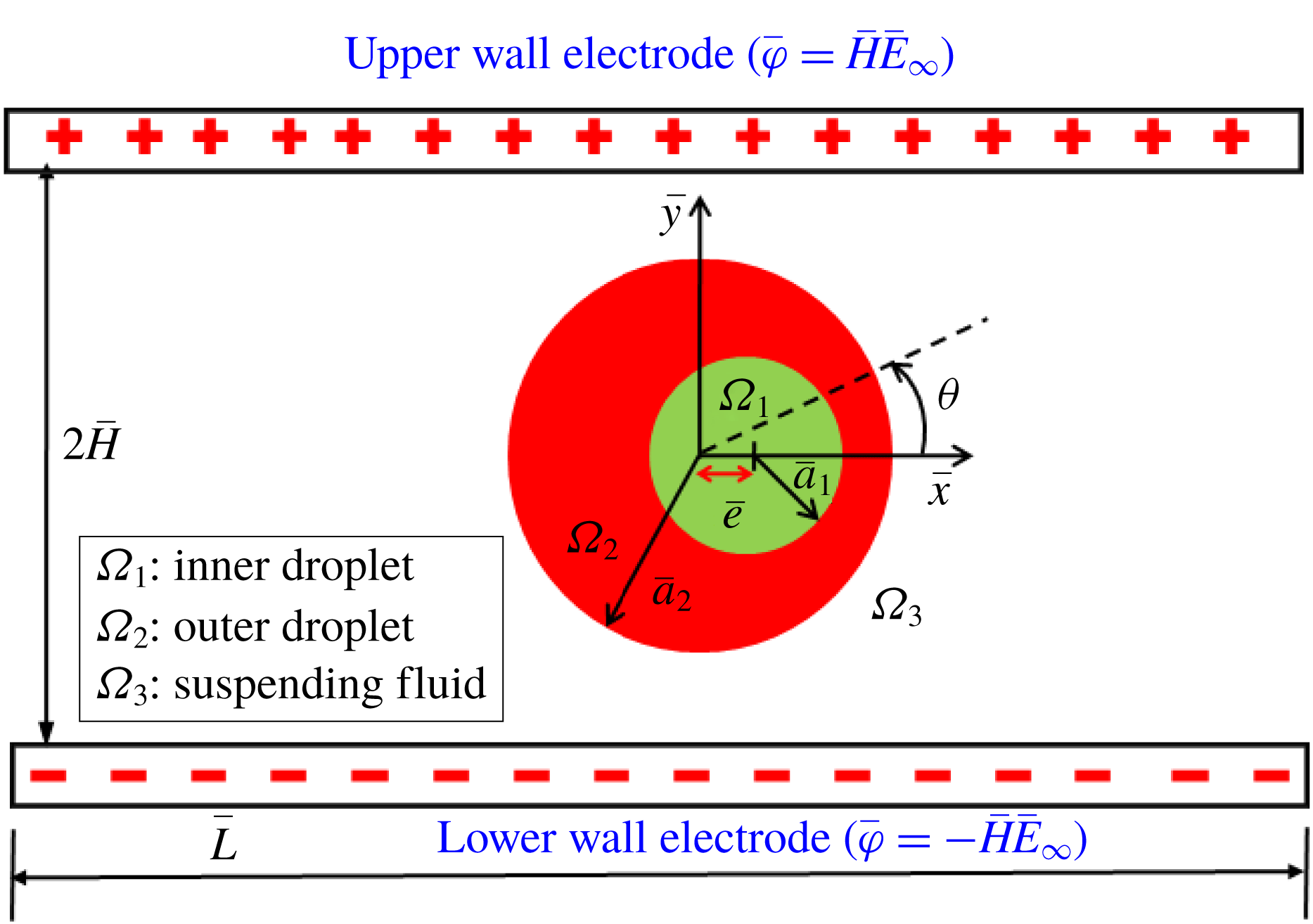
First of all, for affirming the validity of our present numerical model, we have performed the validation of our simulated results for the special case of a single droplet with the experimental results of Tsukada et al. (Reference Tsukada, Katayama, Ito and Hozawa1993) and Salipante & Vlahovska (Reference Salipante and Vlahovska2010) as depicted in figure 3(a). In this figure, we have shown the variation of steady-state deformation parameter with electric field strength (or
 $Ca_{E}$
). The steady-state deformation parameter is used to quantify the magnitude of steady-state deformation and is expressed as
 $D_{\infty }=(D_{max}-D_{min})/(D_{max}+D_{min})$
, where
 $D_{max}$
and
 $D_{min}$
are the semi-major and semi-minor axes of the droplet having approximately elliptical shape (Mahlmann & Papageorgiou Reference Mahlmann and Papageorgiou2009; Mandal et al.
Reference Mandal, Sinha, Bandopadhyay and Chakraborty2018). The comparisons show that the nature of the characteristic curve of steady-state deformation for both cases are similar, where the droplet deforms into oblate and prolate configuration for
 $R<S$
and
 $R>S$
, respectively.
(a) Variation of
 $D_{\infty }$
with
 $Ca_{E}$
. The properties of fluids considered in the study of Tsukada et al. (Reference Tsukada, Katayama, Ito and Hozawa1993) and Salipante & Vlahovska (Reference Salipante and Vlahovska2010) are
 $(R,S)=(62.4,1.72)$
,
 $\unicode[STIX]{x1D706}=1.47$
and
 $(R,S)=(0.027,0.57)$
,
 $\unicode[STIX]{x1D706}=1.40$
, respectively. (b) Transient variation of deformation parameter. Fluid properties are
 $Ca_{E}=0.25$
,
 $\unicode[STIX]{x1D706}=1$
and
 $Re=1$
. (c) Transient variation of deformation parameter. Fluid properties are
 $(R,S)=(30,0.44)$
,
 $Ca_{E}=0.0101$
and
 $\unicode[STIX]{x1D706}=1.846$
.

It is also important to mention that a closer agreement is obtained at lower values of
 $Ca_{E}$
, while the deviation seems to be higher for a comparatively higher values of
 $Ca_{E}$
. Again, we have also made a comparison between our numerically simulated result and the result of Halim & Esmaeeli (Reference Halim and Esmaeeli2013) on the transient deformation characteristic of a droplet for different electrical parameters as depicted in figure 3(b). This figure also shows a very good agreement between our numerical results and the results of Halim & Esmaeeli (Reference Halim and Esmaeeli2013). Additionally, we have compared our numerically simulated result with the analytical result of Esmaeeli & Sharifi (Reference Esmaeeli and Sharifi2011) as illustrated in figure 3(c), which also shows a good agreement. Next, we perform a grid independence study to ensure that the outcomes of the present analysis are independent of the size of the grid element. The details of the grid independence study are given in § 4 of the supplementary material. We next compare the numerical results with our analytical results.
3.1 Comparison between numerical and analytical results
First of all, we have made a comparison between our theoretical prediction and the results obtained from the full-scale numerical simulation. We have performed the theoretical analysis in an unbounded domain, the details of which are shown in § 1 of the supplementary material. In order to attain a greater accuracy in our analytical prediction, we have considered higher-order correction terms in droplet shape. Based on small-deformation perturbation analysis, the inner and outer droplet shapes can be represented as (Mandal et al. Reference Mandal, Ghosh and Chakraborty2016b )
 $$\begin{eqnarray}\left.\begin{array}{@{}c@{}}r_{s_{12}}(\unicode[STIX]{x1D703})=K\{1+f_{12}(\unicode[STIX]{x1D703})\}=K\{1+Ca_{E}\,f_{12}^{(Ca_{E})}+Ca_{E}^{2}\,f_{12}^{(Ca_{E}^{2})}+O(Ca_{E}^{3})\},\\ r_{s_{23}}(\unicode[STIX]{x1D703})=\{1+f_{23}(\unicode[STIX]{x1D703})\}=\{1+Ca_{E}\,f_{23}^{(Ca_{E})}+Ca_{E}^{2}\,f_{23}^{(Ca_{E}^{2})}+O(Ca_{E}^{3})\}.\end{array}\right\}\end{eqnarray}$$
Here
 $f_{ij}^{(Ca_{E})}$
and
 $f_{ij}^{(Ca_{E}^{2})}$
denote the corrections in shape of the interface
 $ij$
at different orders of perturbation, namely
 $O(Ca_{E})$
and
 $O(Ca_{E}^{2})$
, respectively. The corrections can be expressed in the following form as
 $$\begin{eqnarray}O(Ca_{E}):\quad f_{12}^{(Ca_{E})}=M_{2,0}^{(Ca_{E})}\cos (2\unicode[STIX]{x1D703}),\quad f_{23}^{(Ca_{E})}=L_{2,0}^{(Ca_{E})}\cos (2\unicode[STIX]{x1D703}),\end{eqnarray}$$
 $$\begin{eqnarray}O(Ca_{E}^{2}):\quad \left\{\begin{array}{@{}l@{}}f_{12}^{(Ca_{E}^{2})}=M_{0,1}^{(Ca_{E}^{2})}+[M_{2,1}^{(Ca_{E}^{2})}\cos (2\unicode[STIX]{x1D703})+M_{4,1}^{(Ca_{E}^{2})}\cos (4\unicode[STIX]{x1D703})],\\ f_{23}^{(Ca_{E}^{2})}=L_{0,1}^{(Ca_{E}^{2})}+[L_{2,1}^{(Ca_{E}^{2})}\cos (2\unicode[STIX]{x1D703})+L_{4,1}^{(Ca_{E}^{2})}\cos (4\unicode[STIX]{x1D703})],\end{array}\right.\end{eqnarray}$$
where
 $L_{0,1}^{(Ca_{E}^{2})}$
and
 $M_{0,1}^{(Ca_{E}^{2})}$
can again be expressed as
 $$\begin{eqnarray}L_{0,1}^{(Ca_{E}^{2})}=-{\textstyle \frac{1}{4}}\{L_{2,0}^{(Ca_{E})}\}^{2}-{\textstyle \frac{1}{4}}\{\hat{L}_{2,0}^{(Ca_{E})}\}^{2},\quad M_{0,1}^{(Ca_{E}^{2})}=-{\textstyle \frac{1}{4}}\{M_{2,0}^{(Ca_{E})}\}^{2}-{\textstyle \frac{1}{4}}\{\hat{M}_{2,0}^{(Ca_{E})}\}^{2}.\end{eqnarray}$$
The constant coefficients in the above equations are provided in § 2.2 of the supplementary material. The deformation of both of the interfaces can be quantified in terms of a deformation parameter, which can be expressed in the following form:
 $$\begin{eqnarray}D_{ij}=\frac{r_{\unicode[STIX]{x1D6F1}_{ij}}(\unicode[STIX]{x1D703}=\unicode[STIX]{x03C0}/2)-r_{\unicode[STIX]{x1D6F1}_{ij}}(\unicode[STIX]{x1D703}=0)}{r_{\unicode[STIX]{x1D6F1}_{ij}}(\unicode[STIX]{x1D703}=\unicode[STIX]{x03C0}/2)+r_{\unicode[STIX]{x1D6F1}_{ij}}(\unicode[STIX]{x1D703}=0)}.\end{eqnarray}$$
In the present analysis, we have considered two PD–PD–PD (all three phases are perfect dielectric in nature) systems with
 $(S_{23},S_{12})=(10,1)$
and
 $(S_{23},S_{12})=(0.1,10)$
. Three LD–LD–LD systems (here all three phases are leaky dielectric in nature) are also considered where system I is characterized by
 $(S_{23},R_{23})=(0.4397,0.033)$
and
 $(S_{12},R_{12})=(2.274,30.33)$
, system II has
 $(S_{23},R_{23})=(1,10)$
and
 $(S_{12},R_{12})=(1,0.1)$
and finally system III has
 $(S_{23},R_{23})=(2,0.5)$
and
 $(S_{12},R_{12})=(0.5,2)$
. Regarding the selection of
 $\unicode[STIX]{x1D70E}_{1}$
,
 $\unicode[STIX]{x1D70E}_{2}$
and
 $\unicode[STIX]{x1D70E}_{3}$
, it is important to mention that both the conductivity values of the droplet phase and suspending fluid phase can be chosen independently. The conductivity of each fluid phase is constant. However, it varies spatially across the fluid–fluid interface. In the present analysis, the considered values of
 $R_{ij}$
and
 $S_{ij}$
have been extracted from previously performed experimental and numerical studies (Torza et al.
Reference Torza, Cox and Mason1971; Tsukada et al.
Reference Tsukada, Yamamoto, Katayama and Hozawa1994; Mahlmann & Papageorgiou Reference Mahlmann and Papageorgiou2009).
Variation of
 $D_{\infty }$
with
 $Ca_{E}$
for (a) outer droplet and (b) inner droplet of system I with
 $(S_{23},R_{23})=(0.4397,0.033)$
and
 $(S_{12},R_{12})=(2.274,30.33)$
. Other used parameters are
 $Re=0.01$
,
 $\unicode[STIX]{x1D706}=1$
and
 $e=0$
.

(a) Variation of
 $D_{\infty }$
with
 $Wc$
for a PD–PD–PD system at
 $Ca_{E}=0.15$
, (b) droplet shapes for different values of
 $Wc$
, where the blue coloured contour shows the undeformed droplet shape, and (c) variation of
 $E^{2}$
with
 $Wc$
along a vertical line drawn from the droplet centre to the wall electrode. Other parameters are
 $(S_{23},S_{12})=(10,0.1)$
,
 $Re=0.01$
,
 $\unicode[STIX]{x1D706}=1$
and
 $e=0$
.

In order to obtain a good match with our numerical and theoretical results, we have chosen
 $Wc=0.2$
. Here,
 $Wc$
is the ratio of droplet radius and half-height of the channel. Therefore, for a fixed droplet radius, if we decrease the value of
 $Wc$
, it necessarily implies enhancement in channel height. For small values of
 $Wc~({\leqslant}0.2)$
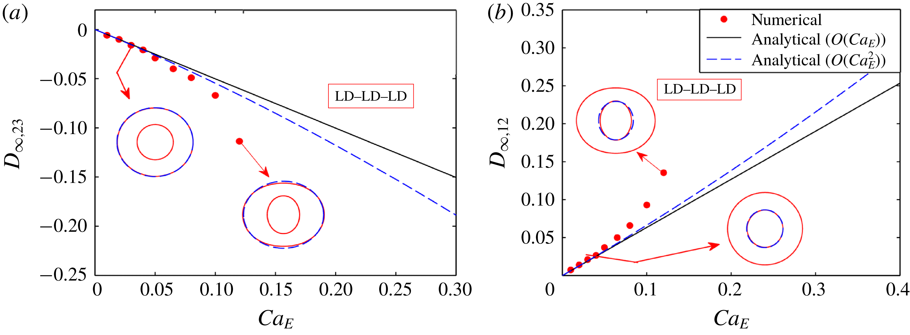
, the channel height is large enough to exclude any interference of it on the dynamics of the droplet and the flow field nearly approximates an unbounded flow field. To ensure this, we have performed a domain confinement independence test. The details of this test are given in § 5 of the supplementary material. In figure 4, we show the variation of steady-state deformation parameter
 $(D_{\infty })$
with
 $Ca_{E}$
both numerically and analytically. Figure 4(a,b) depicts the variation of
 $D_{\infty ,23}$
and
 $D_{\infty ,12}$
with
 $Ca_{E}$
for the outer and inner droplet of an LD–LD–LD model (system I). Droplet shapes corresponding to different values of
 $Ca_{E}$
are also shown in figure 4. The plots in figure 4 show that the leading-order (
 $O(Ca_{E})$
correction in shape) and higher-order (
 $O(Ca_{E}^{2})$
correction in shape) asymptotic theory corroborates well with the numerical results for lower values of
 $Ca_{E}~({\leqslant}0.04)$
. However, for a relatively larger value of
 $Ca_{E}$
(
 $=0.08$
, for illustration), the higher-order asymptotic analysis shows better agreement with the numerically obtained results as compared to the leading-order theoretical prediction. This can be explained by looking into (3.1), which implies that, for lower values of
 $Ca_{E}$
, the leading-order term dominates. Therefore, the magnitudes of steady-state deformation obtained from leading-order and higher-order asymptotic analysis are small and are virtually the same. However, if we increase the value of
 $Ca_{E}$
, the higher-order terms start contributing in dictating the deformation. Hence, we observe a substantial difference between the results obtained from leading-order and higher-order asymptotic analysis and the latter shows better agreement with the numerical results. As the asymptotic analysis offers approximate solution, it is very hard to achieve a point-to-point matching between the numerical and the analytical results for large values of
 $Ca_{E}$
. Similar characteristics are also observed for the PD–PD–PD system.
3.2 Channel confinement-induced variation in steady-state deformation
3.2.1 Fluid systems with equal viscosity
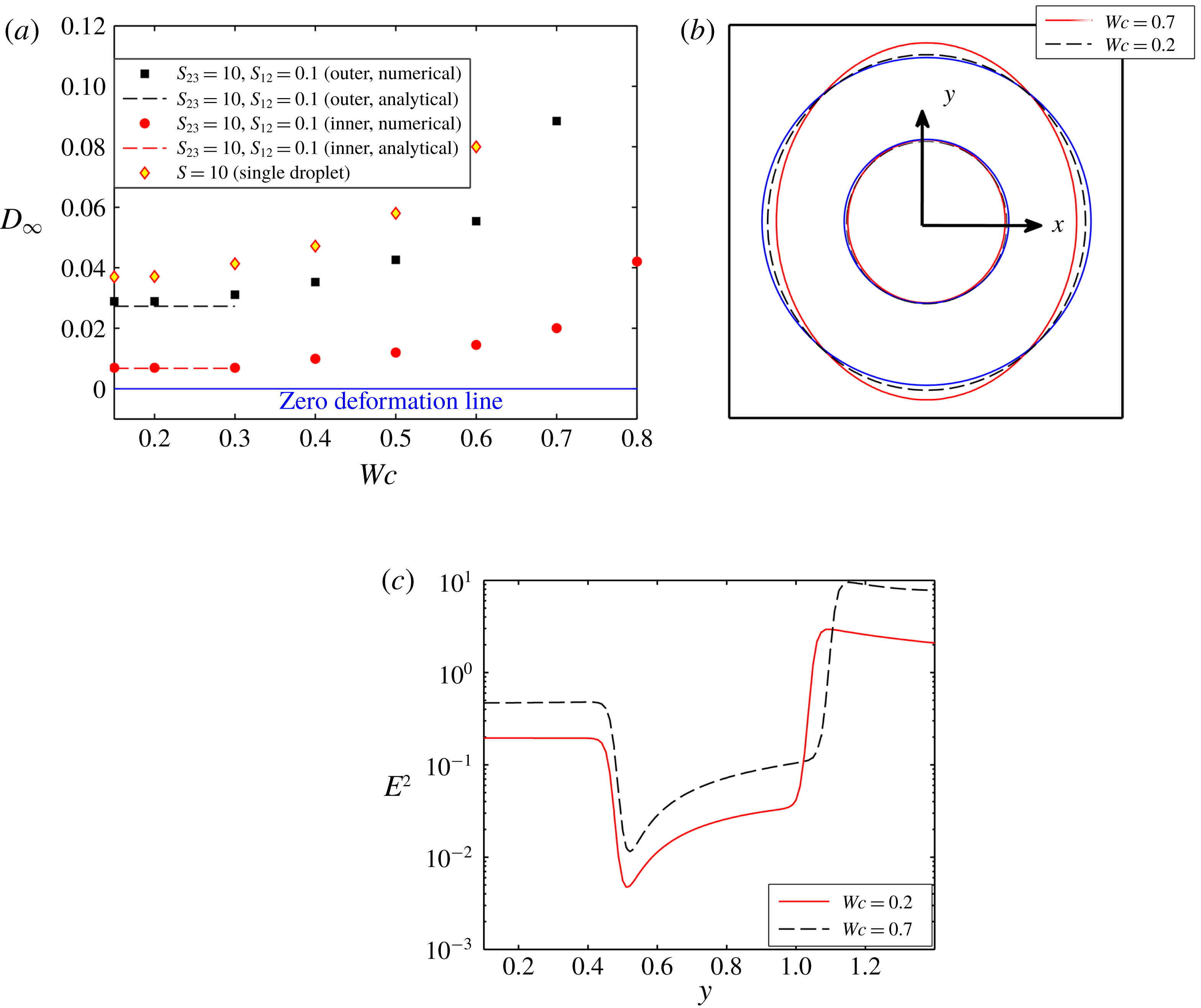
Figure 5 shows the effect of channel confinement on the steady-state deformation of a compound droplet for a PD–PD–PD system with
 $(S_{23},S_{12})=(10,0.1)$
. The channel confinement ratio is varied between
 $Wc=0.2$
and
 $Wc=0.8$
to obtain a better understanding of the effect of the bounding wall. From figure 5(a), it can be observed that the steady-state deformation of both the inner and outer droplet increases with rise in the channel confinement. Both interfaces are deformed into a prolate shape, which is evident from figure 5(b). The primary reason for such a behaviour is due to the rise in strength of the electric field with increase in the domain confinement. Figure 5(c) shows that the magnitude of the electric field strength is high for a highly confined domain. Therefore, the magnitude of normal electric stress is also high, which results in an enhanced deformation of the droplet. It is also important to note that the outer droplet undergoes a greater droplet deformation as compared to the inner droplet. Such a behaviour can be attributed to the following two reasons: (i) the permittivity of the inner droplet is low and as a result lower Maxwell stress is generated at the interface, and (ii) the restoring force of the inner droplet is much more significant due to lower interfacial curvature. Another important aspect to be noted is that the deformation of the outer droplet is less in comparison to a single droplet. As the permittivity of the inner droplet is less, the Maxwell stress generated at the inner interface is small, which creates a lower deformation of the interface. Therefore, the intensity of the viscous flow (and hence the viscous stress) at the annular region, generated due to the deformation of the inner interface, is also weak, which causes lower deformation of the outer interface. This analysis is also true for a PD–PD–PD system with
 $S_{23}<1$
and
 $S_{23}>1$
.
Similarly, figure 6(a) demonstrates the variation of steady-state deformation parameter as a function of the domain confinement for the leaky dielectric system II with
 $(R_{23}>S_{23})$
and
 $(R_{12}<S_{12})$
. Figure 6(a) demonstrates that the steady-state deformation of the inner droplet reduces with rise in the confinement ratio, whereas the deformation of the outer droplet increases till
 $Wc=0.80$
. Any further increase in the channel confinement results in a reduction in the deformation of the outer droplet. For a leaky dielectric system, the deformation dynamics of the droplet is mainly regulated by the interplay between normal electric and hydrodynamic stress. In an unbounded domain, these stresses act in the same direction and try to deform the outer droplet
 $(R_{23}>S_{23})$
and inner droplet
 $(R_{12}<S_{12})$
into prolate and oblate configurations, respectively. It is worth mentioning that the confinement effect induces higher electric potential in a confined domain and increases the electric field strength as depicted in figure 6(b). Therefore, with the rise in the domain confinement, the normal electric stress increases, which enhances the deformation.
(a) Variation of
 $D_{\infty }$
with
 $Wc$
for system II with
 $(S_{23},R_{23})=(1,10)$
and
 $(S_{12},R_{12})=(1,0.1)$
at
 $Ca_{E}=0.1$
, and (b) variation of
 $E^{2}$
with
 $Wc$
along a vertical line drawn from the droplet centre to the wall electrode. Other used parameters are
 $Re=0.01$
,
 $\unicode[STIX]{x1D706}=1$
and
 $e=0$
.

On the contrary, the magnitude of the normal hydrodynamic stress decreases with domain confinement ratio
 $(Wc)$
, and beyond a certain critical value of
 $Wc$
, it becomes reverse. We have described it as the critical confinement ratio
 $(Wc_{critical})$
. Further increment of the channel confinement increases the magnitude of reversed hydrodynamic stress, which now tries to oppose the effect of the normal electric stress. For the outer droplet, as the value of
 $R_{23}$
is high, the effect of domain confinement on the normal electric stress is also high and it dominates the decrease in normal hydrodynamic stress till
 $Wc=0.80$
.
(a) Variation of
 $D_{\infty }$
with
 $Wc$
for system I with
 $(S_{23},R_{23})=(0.4397,0.033)$
and
 $(S_{12},R_{12})=(2.274,30.33)$
at
 $Ca_{E}=0.08$
, and (b) droplet shapes for different values of
 $Wc$
where the blue coloured contour shows the undeformed droplet shape. Other used parameters are
 $Re=0.01$
,
 $\unicode[STIX]{x1D706}=1$
and
 $e=0$
.

Increase in
 $Wc$
beyond the value of 0.8 reverses the direction of the normal hydrodynamic stress as well as increases its magnitude significantly such that a reduction in shape deformation of the outer interface results. For the present LD–LD–LD model too, the deformation of the inner droplet is lower as compared to the outer droplet because of the lower conductivity and a higher restoring force of the inner droplet. Like the PD–PD–PD model, the steady-state deformation of the outer droplet of the present system is smaller than that of a single droplet due to the presence of the inner droplet.
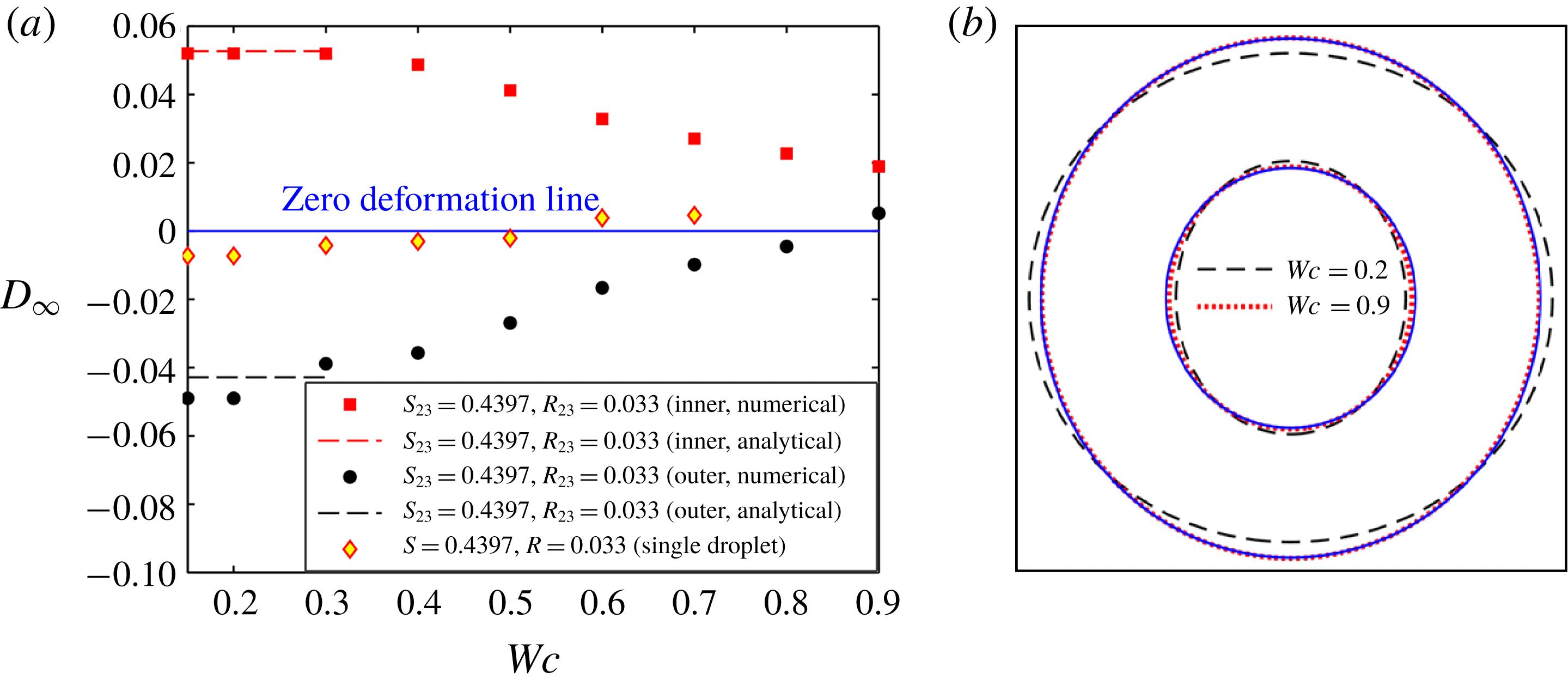
Similarly, figure 7 shows the alteration of steady-state deformation parameter with domain confinement for system I having
 $(R_{23}<S_{23})$
and
 $(R_{12}>S_{12})$
. From figure 7(a), it can be noted that the inner and outer droplet deform into a prolate and an oblate configuration, respectively, in an unbounded domain. With the rise in channel confinement, the steady-state value of the deformation parameter of both interfaces (inner and outer) decreases. When the droplet is highly confined in the channel, that is
 $Wc\geqslant 0.8$
, both interfaces deform into a prolate configuration, which is clearly understood from figure 7(b). This phenomenon happens because of the critical interplay between normal electric and normal hydrodynamic stresses in a confined domain. In the case of a leaky dielectric system, the strength of normal electric stress increases with domain confinement similar to system II. On the other hand, the normal hydrodynamic stress decreases, and above a critical domain confinement, it gets reversed, as mentioned in the study of Esmaeeli & Behjatian (Reference Esmaeeli and Behjatian2012) and Santra et al. (Reference Santra, Mandal and Chakraborty2018). For the outer droplet, the increase in normal electric stress with domain confinement is less as compared to the reduction in normal hydrodynamic stress, as the conductivity ratio is low
 $(R_{23})$
. So, the steady-state deformation of the outer droplet reduces, and beyond
 $Wc\approx 0.80$
, the reversed normal hydrodynamic stress dominates the normal electric stress, which leads the droplet to deform into a prolate configuration. We also observe that the critical confinement ratio
 $(Wc_{critical}\approx 0.8)$
is higher as compared to a single droplet
 $(Wc\approx 0.55)$
due to the presence of the inner droplet. For the present LD–LD–LD model, the surface charge induced at the inner droplet interface is higher due to the large magnitude of
 $R_{12}$
. So, the viscous flow generated due to the disparity in the tangential electric stresses is also high, which increases the deformation of both interfaces. In addition, the Maxwell stress induced at the inner droplet interface is also large, which creates a significantly higher prolate deformation of the inner droplet. As a consequence, the flow in the annular region becomes squeezed, which increases the strength of the viscous stress at both interfaces and further enhances the deformation. Hence, the oblate deformation of the outer droplet is significantly higher as compared to a single droplet and the transformation of droplet shape from oblate to prolate configuration takes place at comparatively higher domain confinement ratios.
3.2.2 Fluid system with different viscosities
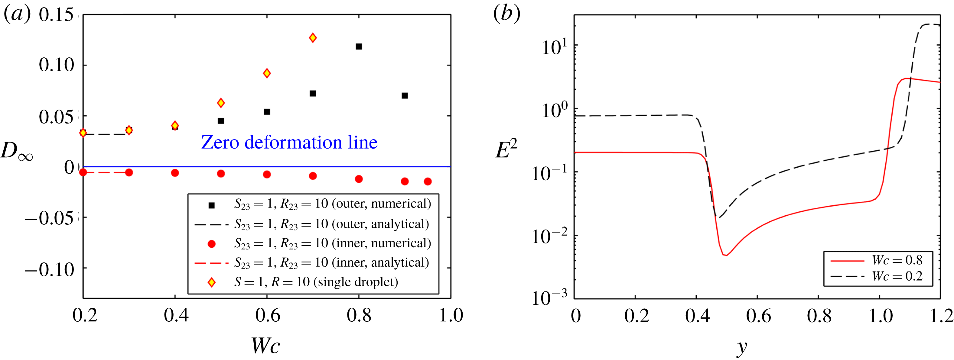
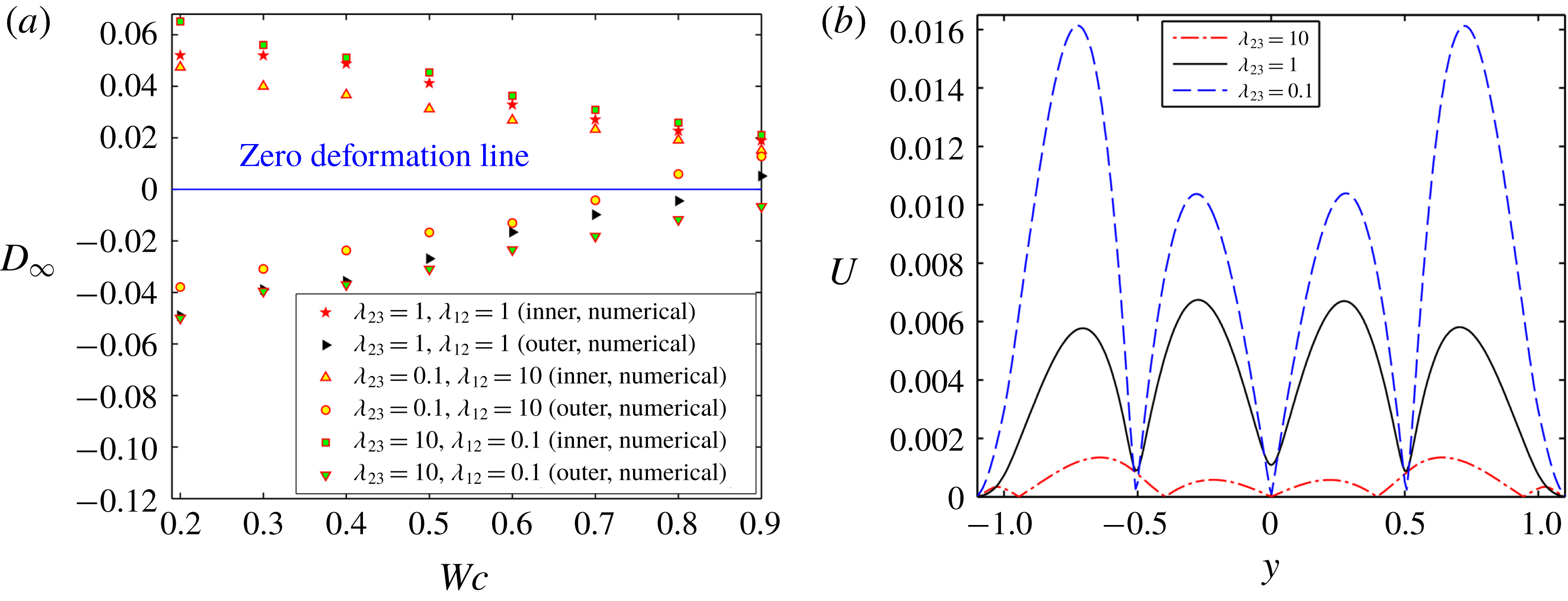
Next, figure 8(a) shows the effect of viscosity ratio on the variation of
 $D_{\infty }$
with
 $Wc$
for LD–LD–LD system I (having
 $R_{23}<S_{23}$
and
 $R_{12}>S_{12}$
). From figure 8(a), it is understood that the deformation of both the droplets is higher for higher values of
 $\unicode[STIX]{x1D706}_{23}$
in a weakly confined domain. This happens due to increase in hydrodynamic stress in the annular region. In contrast to an unbounded domain, the deformation of the outer droplet is greater for lower values of
 $\unicode[STIX]{x1D706}_{23}$
in a confined domain. On the other hand, the deformation of the inner droplet remains higher for higher values of
 $\unicode[STIX]{x1D706}_{23}$
in a confined domain. The reason behind the observed phenomenon is now provided. For the present LD–LD–LD system, in a confined domain, the normal hydrodynamic stress acts in the opposite direction to the normal electric stress and plays a dominating role in determining the degree of deformation of the outer droplet. From figure 8(b), it is observed that the magnitude of velocity is higher for lower values of
 $\unicode[STIX]{x1D706}_{23}$
, which necessarily implies a higher magnitude of normal hydrodynamic stress, which causes more prominent prolate deformation of the outer droplet. Again, the effect of the normal hydrodynamic stress on the deformation of the inner droplet is comparatively less significant as compared to the outer droplet in a confined domain due to the higher magnitude of the normal electric stress and the restoring force.
Effect of viscosity ratio on (a) the variation of
 $D_{\infty }$
with
 $Wc$
, and (b) the variation of velocity magnitude for
 $Wc=0.8$
and
 $t=10$
along a vertical line passing through the centre of the droplet and drawn from lower to upper electrode for system I. Other used parameters are
 $(S_{23},R_{23})=(0.4397,0.033)$
and
 $(S_{12},R_{12})=(2.274,30.33)$
,
 $Ca_{E}=0.08$
,
 $Re=0.01$
and
 $e=0$
.

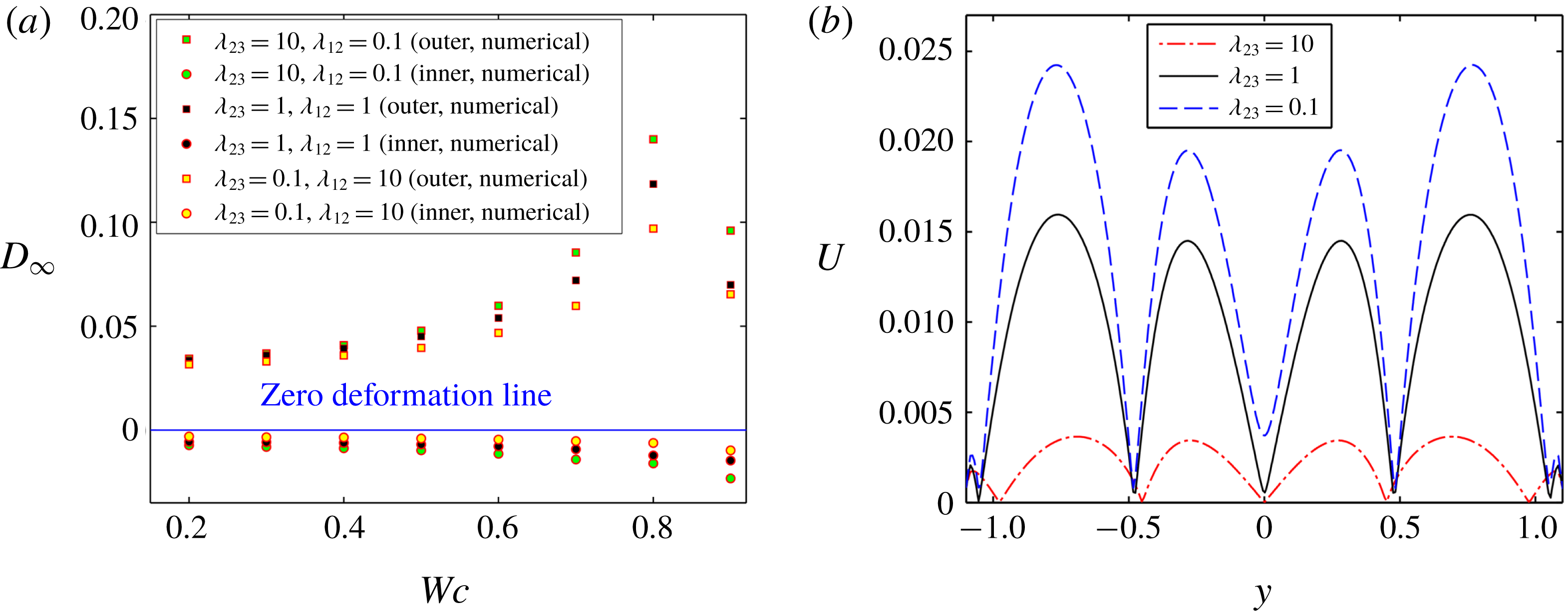
A similar observation is reflected in figure 9(a) for the LD–LD–LD system II (having
 $R_{23}>S_{23}$
and
 $R_{12}<S_{12}$
). For the present LD–LD–LD system, as the value of
 $R_{23}$
is high, the magnitude of normal electric stress is also high and it thus regulates the deformation dynamics of the droplet, where the normal hydrodynamic stress only strengthens and weakens the magnitude of normal electric stress in unbounded and confined domain, respectively. From figure 9(a), it can be seen that the deformation of both the droplets increases with rise in the values of viscosity ratio. The effect of viscosity ratio is more prominent in a confined domain.
Effect of viscosity ratio on (a) the variation of
 $D_{\infty }$
with
 $Wc$
, and (b) the variation of velocity magnitude at
 $Wc=0.8$
and
 $t=10$
along a vertical line passing through the centre of the droplet and drawn from lower to upper electrode for system II with
 $(S_{23},R_{23})=(1,10)$
and
 $(S_{12},R_{12})=(1,0.1)$
at
 $Ca_{E}=0.1$
.

The reason behind the observed phenomenon is discussed now. For the present LD–LD–LD system in a confined domain, the normal hydrodynamic stress acts in the opposite direction to the normal electric stress and tries to reduce the prolate deformation caused by the normal electric stress. From figure 9(b), it is observed that, in a confined domain, the magnitude of velocity is lower for higher values of viscosity ratio
 $(\unicode[STIX]{x1D706}_{23})$
. This implies that the effect of normal hydrodynamic stress is also minimal for higher values of viscosity ratio, which causes lower reduction of the normal electric stress. For that reason, the value of the steady-state deformation parameter is significantly higher for larger values of viscosity ratio in a confined domain.
3.2.3 Droplet morphology in combined presence of domain confinement and electrical forcing
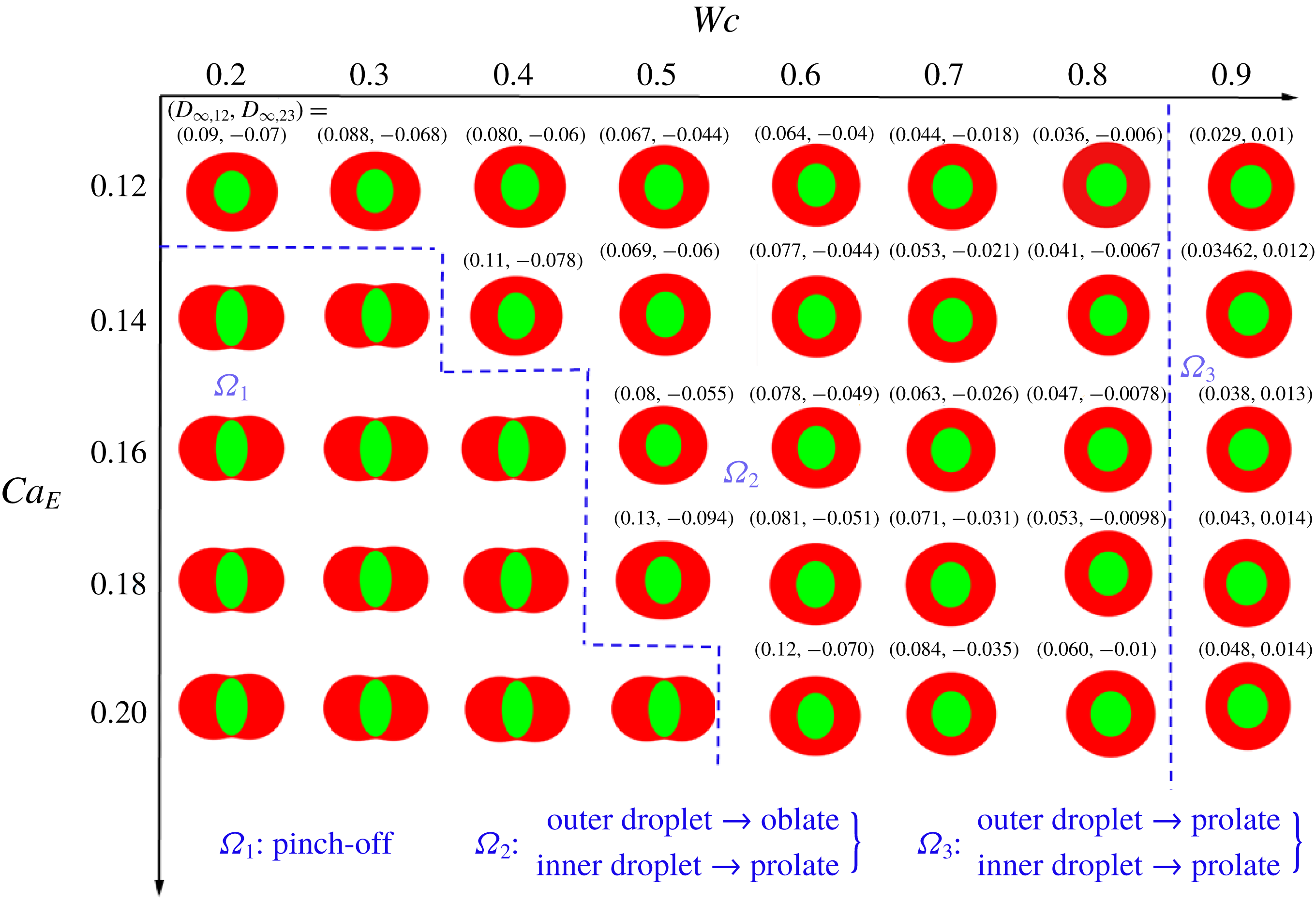
Next, we have constructed a regime diagram in figure 10 to show the dependence of droplet shape on the channel confinement
 $(Wc)$
and the electric capillary number
 $(Ca_{E})$
.
Regime diagram showing three different regimes of droplet deformation. Other parameters are
 $(S_{23},R_{23})=(0.4397,0.033)$
,
 $(S_{12},R_{12})=(2.274,30.33)$
,
 $Re=0.01$
,
 $\unicode[STIX]{x1D706}=1$
and
 $e=0$
.

Figure 10 identifies three distinct regimes of steady-state droplet deformation: (i) regime
 $\unicode[STIX]{x1D6FA}_{1}$
, where the droplet undergoes a pinch-off phenomenon, (ii) regime
 $\unicode[STIX]{x1D6FA}_{2}$
, where the outer droplet deforms into an oblate shape and the inner droplet deforms into a prolate shape, and (iii) regime
 $\unicode[STIX]{x1D6FA}_{3}$
, where both droplets deform into a prolate configuration. In a weakly confined domain, the outer and inner droplets deform into oblate and prolate configurations, respectively, for lower values of
 $Ca_{E}$
. A slight increment in
 $Ca_{E}$
, however, leads to pinch-off of the inner droplet.
Now, we will provide a detailed explanation of the observed phenomenon. In regime
 $\unicode[STIX]{x1D6FA}_{1}$
, the normal electric stress and the normal hydrodynamics stress act in the same direction. Furthermore, the magnitude of these forces is also significantly high as the considered values of
 $Ca_{E}$
are high. The combined effect of these forces tries to stretch the inner droplet in the direction of the electric field and the outer droplet perpendicular to the applied electric field, which leads to the occurrence of a pinch-off phenomenon. However, this pinch-off tendency reduces with increase in the domain confinement and the droplet achieves a steady-state configuration in regime
 $\unicode[STIX]{x1D6FA}_{2}$
. This phenomenon can be explained by the fact that the strength of the normal hydrodynamic stress decreases with the increase in domain confinement
 $(Wc)$
. After a certain value of
 $Wc~(=Wc_{critical}\approx 0.8)$
, both interfaces deform into a prolate configuration as depicted in
 $\unicode[STIX]{x1D6FA}_{3}$
. The reason is that the normal hydrodynamic stress becomes reversed in the regime
 $\unicode[STIX]{x1D6FA}_{3}$
. Now, for the considered values of permittivity ratio and conductivity ratio, the reversed normal hydrodynamic stress becomes dominating in the outer interface, which causes the prolate deformation of the outer droplet. However, in the inner interface, the strength of the normal electric stress is higher as compared to the reversed normal hydrodynamic stress as
 $R_{12}\gg S_{12}$
. Therefore, the inner droplet still deforms into a prolate configuration.
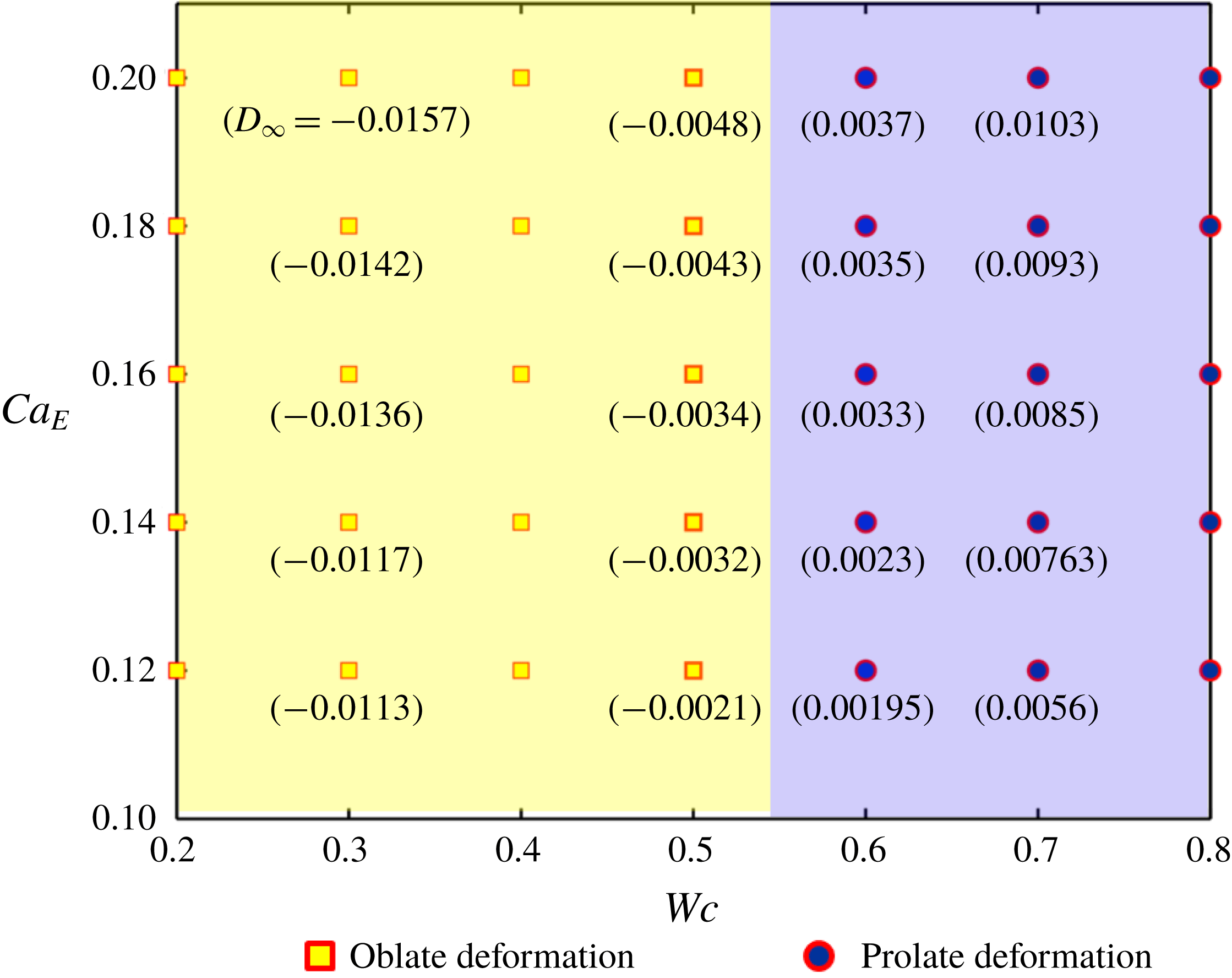
Furthermore, we have constructed a similar regime diagram for a single droplet, shown in figure 11. Comparing figures 10 and 11, it is found that a single droplet retains its steady-state configuration in an unbounded domain, even at sufficiently high values of
 $Ca_{E}$
, unlike a compound droplet. That is, the pinch-off (or breakup) phenomenon for a single droplet is absent in the range of values considered for
 $Ca_{E}$
. This phenomenon can be explained by illustrating the effect of the inner droplet on the deformation of the compound droplet. For the considered values of electrical conductivity and permittivity ratio
 $(R_{12}\gg S_{12})$
, the induced surface charge density at the inner interface is greater. Therefore, the magnitude of EHD flow created due to the mismatch in the tangential electric stresses is also greater. This enhances the deformation of both interfaces. Furthermore, the strength of the normal electric stress on the interface of the inner droplet is also high, which creates considerably larger prolate deformation of the inner droplet. As a result, the flow in the annular region becomes squeezed and induces a very high viscous stress on both interfaces, which enhances the deformation and finally leads to the pinch-off of the compound droplet.
Regime diagram showing three different regimes of droplet deformation. Other parameters are
 $(S,R)=(0.4397,0.033)$
,
 $Re=0.01$
and
 $\unicode[STIX]{x1D706}=1$
.

Temporal variation of deformation parameter for (a) inner droplet, and (b) outer droplet of system I with
 $(S_{23},R_{23})=(0.4397,0.033)$
and
 $(S_{12},R_{12})=(2.274,30.33)$
. Other parameters are
 $Wc=0.2$
,
 $Re=0.01$
,
 $\unicode[STIX]{x1D706}=1$
and
 $e=0$
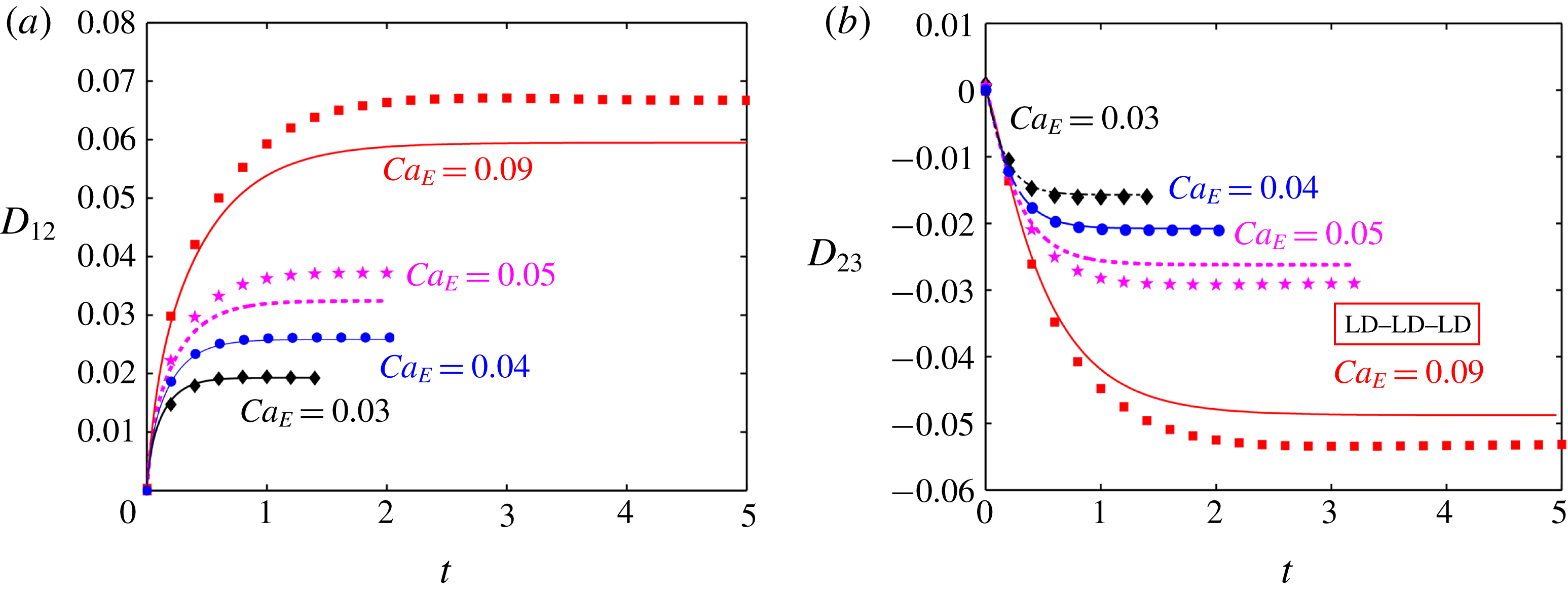
. In these plots, the markers show the numerical results and the lines show the analytical results.

3.3 Channel confinement-induced variation in transient deformation characteristics
3.3.1 Fluid system having equal viscosities
Figure 12 depicts the temporal evolution of the deformation parameter for different values of
 $Ca_{E}$
in a weakly confined domain
 $(Wc=0.2)$
. One must acknowledge that time is normalized with the scale
 $\overline{a}_{2}/\overline{u}_{c}$
in all the transient plots.
In these plots, we have plotted the numerical data and compared them with the theoretical predictions. Figure 12(a,b) shows the variation of deformation parameter for the inner and outer droplet of an LD–LD–LD system (system I). At lower values of
 $Ca_{E}$
, all the plots show a good match between the analytical and numerical results. However, the analytical solution overpredicts the deformation of the outer droplet and underpredicts the deformation of the inner droplet for system I.
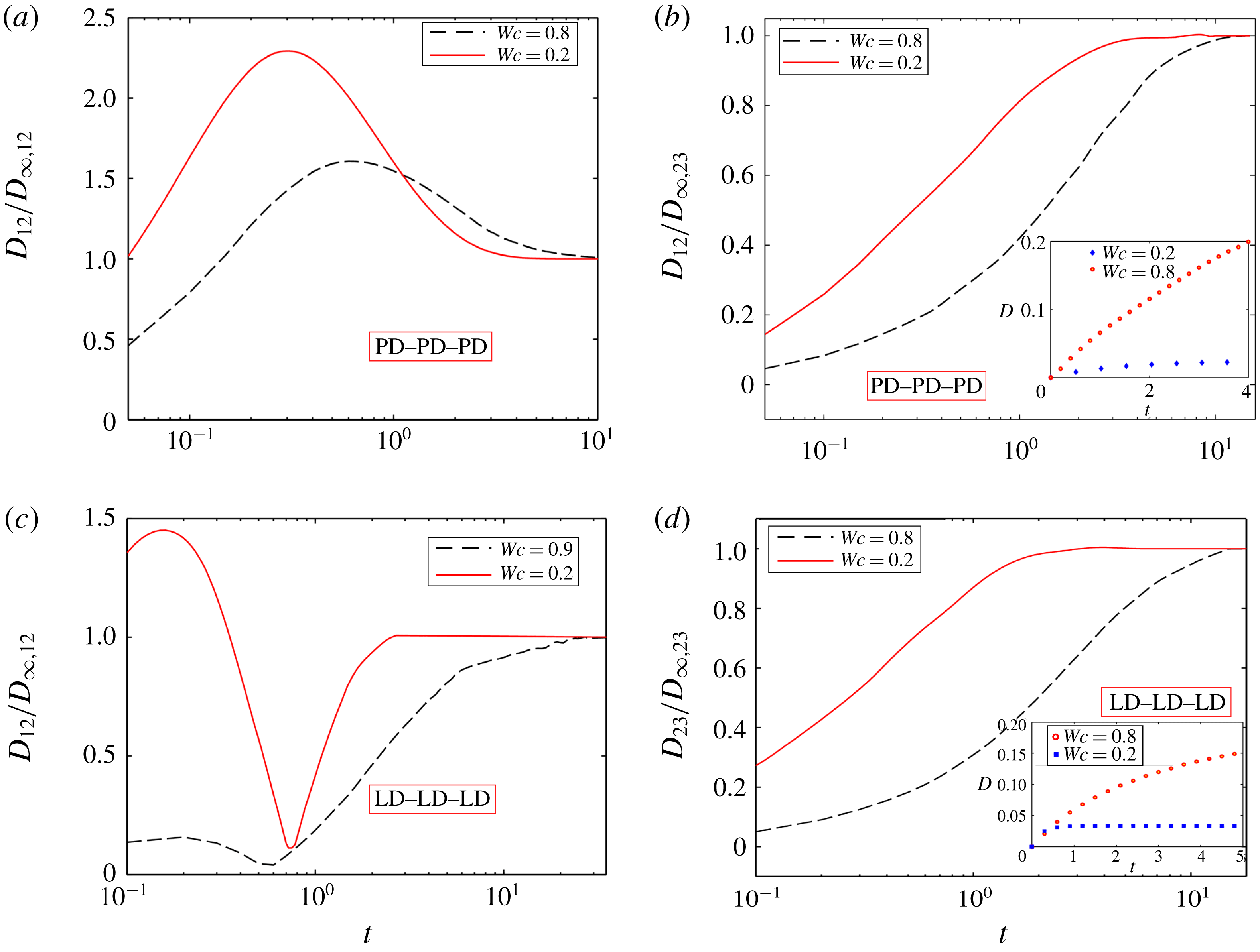
In this section, we have also shown the effect of domain confinement on the time required to attain the steady-state shape (or steady-state time) of the inner and outer droplet of a PD–PD–PD system with
 $(S_{23},S_{12})=(10,0.1)$
and LD–LD–LD system (system II) in figure 13.
Impact of confinement on the steady-state time for (a) the inner droplet, (b) outer droplet of a PD–PD–PD system with
 $(S_{23},S_{12})=(10,0.1)$
, (c) inner droplet at
 $Ca_{E}=0.15$
, and (d) outer droplet of system II with
 $(S_{23},R_{23})=(1,10)$
and
 $(S_{12},R_{12})=(1,0.1)$
at
 $Ca_{E}=0.1$
. The insets in panels (b) and (d) show the variation of the same for a single droplet. Other parameters are
 $Re=0.01$
,
 $e=0$
and
 $\unicode[STIX]{x1D706}=1$
.

Figure 13(a,c) shows a non-monotonic variation of the deformation parameter of the inner droplet as a function of time elapsed for both a perfect and a leaky dielectric system, respectively. In either of these systems, a weakly confined compound droplet reaches its steady-state configuration earlier as compared to a tightly confined one. On the other hand, figure 13(b,d) shows the transient variation of the deformation parameter of the outer droplets of a PD–PD–PD and an LD–LD–LD system. For both these systems, the deformation parameter undergoes a monotonic variation and the droplets achieve a steady-state configuration very sluggishly in the presence of confinement, which increases the steady-state time. This happens due to greater deformation of the droplet in a confined domain. For greater deformation of the droplet, higher interfacial curvature values are locally needed for balancing the shear stress, which raises the steady-state time. An important point to note is that a single droplet undergoes a drastic elongation that leads to its breakup for the same values of
 $R$
,
 $S$
and
 $Ca_{E}$
unlike the outer interface of the compound droplet (refer to the insets of figure 13
b,d). This behaviour is primarily due to the lower conductivity (for an LD–LD–LD system) or permittivity (for a PD–PD–PD system) of the inner droplet. For the present PD–PD–PD system, as the value of
 $S_{12}$
is low, the Maxwell stress generated at the interface is also less, which results in lower deformation of the inner surface. Hence, the strength of the viscous flow generated due to the deformed interface is also weak, which reduces the deformation of the outer interface. For that reason, the outer droplet is able to sustain its steady-state configuration at comparatively higher values of
 $Ca_{E}$
, unlike a single droplet. A similar explanation is also applicable for the present LD–LD–LD system, where the presence of the inner droplet and its prolate deformation reduce the deformation of the outer droplet and help the outer droplet to achieve a steady-state configuration at comparatively higher value of
 $Ca_{E}$
.
3.3.2 Fluid system having different viscosities
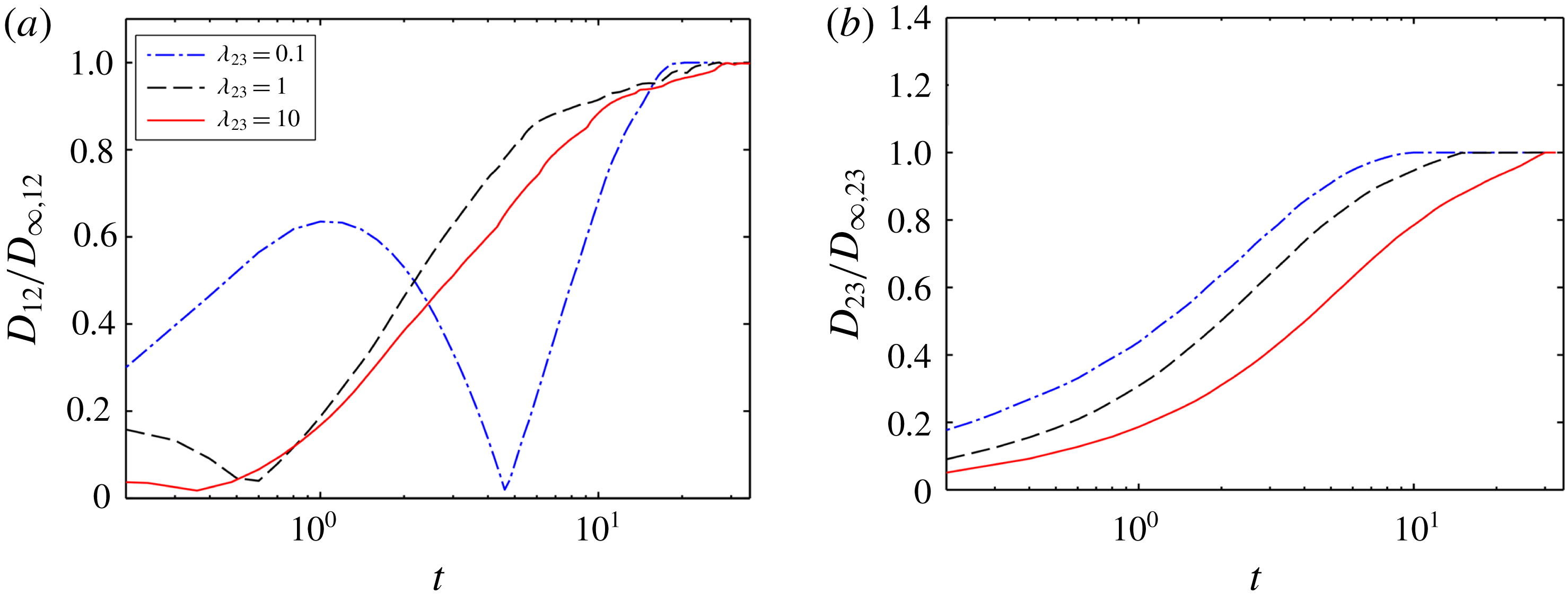
Next, we have shown the effect of viscosity ratio on the time required to achieve the steady-state configuration (or steady-state time) of the inner and outer droplet of the LD–LD–LD system II with
 $(S_{23}<R_{23})$
and
 $(S_{12}>R_{12})$
in a confined domain as shown in figure 14(a,b), respectively. From figure 14, it can be inferred that the time for attaining steady state of both the inner and outer droplet enhances with increase in the values of viscosity ratio. From figure 9(a), it was observed that the steady-state deformation of the inner and outer droplet increased with the rise of the values of viscosity ratio
 $(\unicode[STIX]{x1D706}_{23})$
.
Impact of viscosity ratio on the steady-state time for (a) the inner droplet, and (b) outer droplet of LD–LD–LD system II with
 $(S_{23},R_{23})=(1,10)$
and
 $(S_{12},R_{12})=(1,0.1)$
in a confined domain. Other parameters are
 $Ca_{E}=0.1$
,
 $Re=0.01$
and
 $e=0$
.

As the deformation of the droplet is more for higher viscosity ratio, the droplet necessitates a higher interfacial curvature for balancing the shear stress, which enhances the time to reach steady-state configuration. Similar results are obtained for the PD–PD–PD system (
 $S_{23}>1$
and
 $S_{12}<1$
or
 $S_{23}<1$
and
 $S_{12}>1$
) and LD–LD–LD system I with
 $(S_{23}>R_{23})$
and
 $(S_{12}<R_{12})$
.
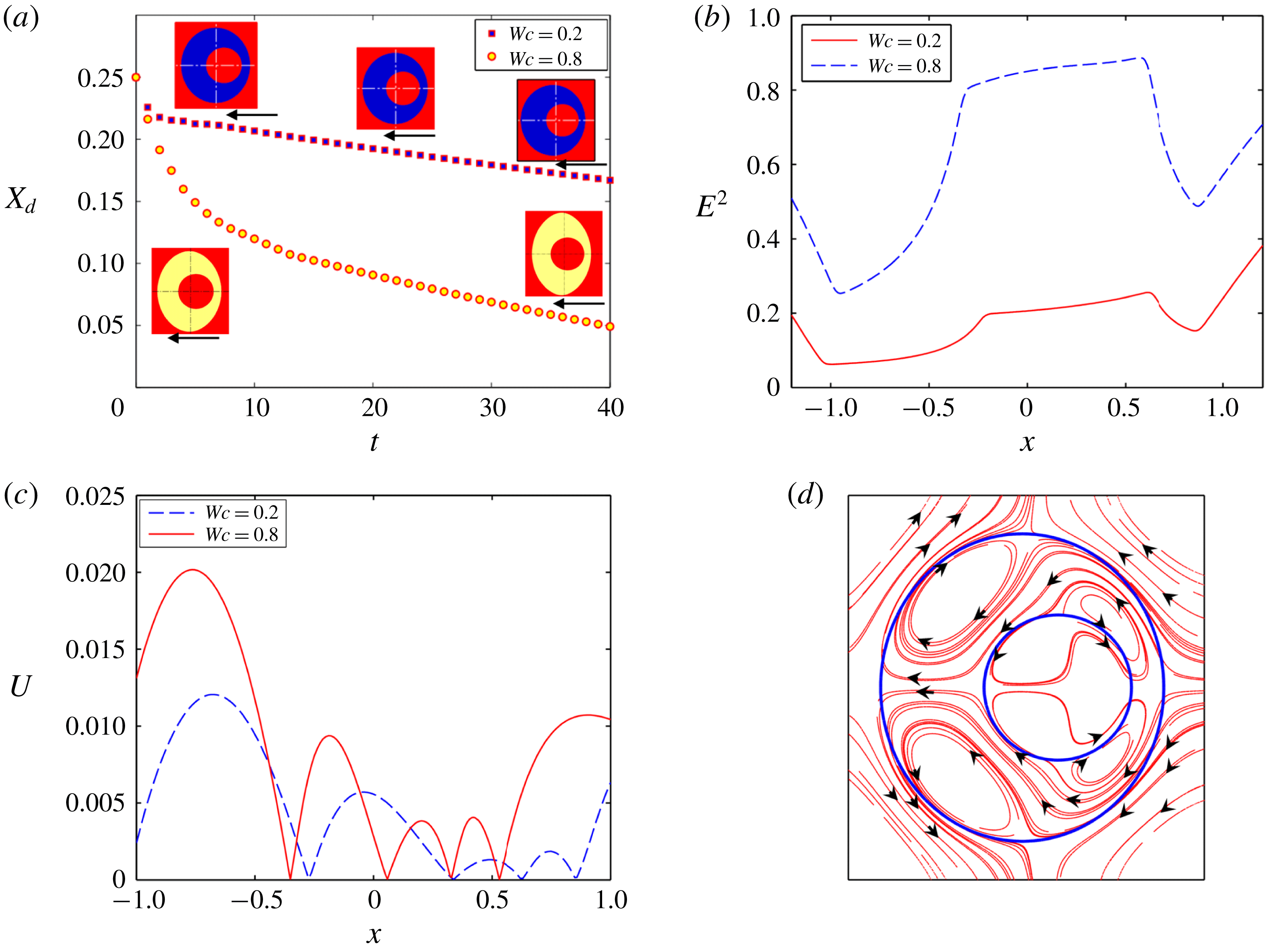
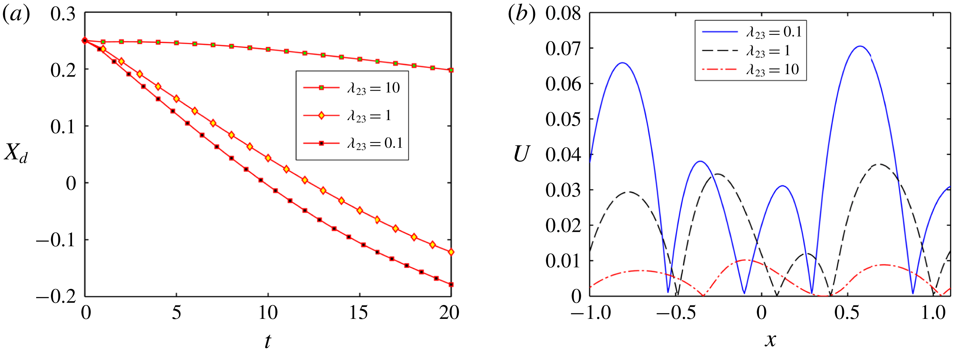
Impact of confinement on (a) the temporal variation of the position of the inner droplet for system II, (b) variation of
 $E^{2}$
along straight horizontal line passing through the centre of the droplets from west pole to east pole of the outer droplet at
 $t=10$
, (c) variation of
 $U$
along a straight horizontal line passing through the centre of the droplets from west pole to east pole of the outer droplet at
 $t=10$
, and (d) streamline pattern of fluid flow circulation at
 $Wc=0.2$
. Other parameters are
 $Re=0.01$
,
 $Ca_{E}=0.125$
,
 $(S_{23},R_{23})=(1,10)$
,
 $(S_{12},R_{12})=(1,0.1)$
,
 $e=0.25$
and
 $\unicode[STIX]{x1D706}=1$
.

3.4 Effect of eccentricity of the inner droplet on its motion
3.4.1 Fluid system having equal viscosity
This section is devoted to investigate the motion of an eccentrically placed inner droplet in the presence of a uniform electric field. The motion of the inner droplet comes into play due to the following two forces: (i) the dielectrophoretic force and (ii) the EHD force. The dielectrophoretic force is expressed as
 $F_{D}=-(1/2)E^{2}\boldsymbol{\cdot }\unicode[STIX]{x1D735}\unicode[STIX]{x1D700}$
and is generated due to the non-uniformity of electrical permittivity of the system. On the other hand, the EHD force is generated due to the asymmetric distribution of the fluid flow around the inner droplet. It is important to mention that, for a concentric droplet, the net dielectrophoretic force and the EHD force acting on the inner droplet along the direction of the electric field is also zero. Hence the inner droplet does not exhibit any motion towards the direction of the electric field (refer to § 6 of the supplementary material for details).
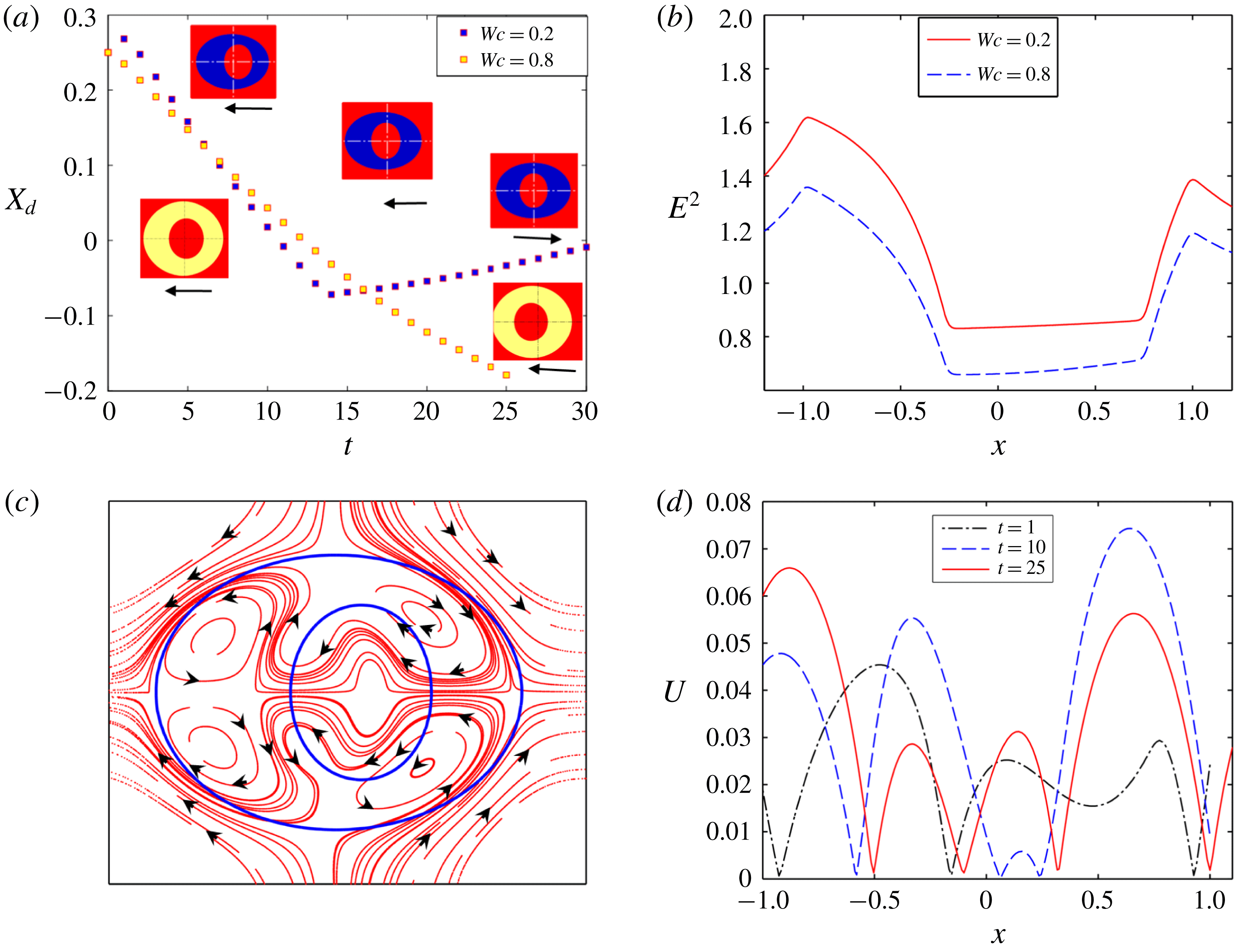
In figure 15(a), we have shown the axial motion of the inner droplet of system II with
 $(S_{23}<R_{23})$
and
 $(S_{12}>R_{12})$
in both confined and unbounded domains. This motion is possible due to the non-uniform distribution of electric field and fluid flow along the axial direction as shown in figure 15(b,c), respectively. From figure 15(a), it should be noted that the translational motion of the inner droplet takes place towards the west pole
 $(\unicode[STIX]{x1D703}=\unicode[STIX]{x03C0})$
of the outer droplet in both a confined and an unbounded domain. It has been previously mentioned that the translational motion of the inner droplet depends on the imbalance of EHD force and dielectrophoretic force. From figure 15(b), it is seen that the magnitude of
 $E^{2}$
is higher at the right side of the inner droplet compared to the left side. Again, the magnitude of electric field strength inside the inner droplet is higher compared to the annular region. Thus, the dielectrophoretic force on the inner droplet acts towards the west pole
 $(\unicode[STIX]{x1D703}=\unicode[STIX]{x03C0})$
of the outer droplet and tries to move the inner droplet in that same direction. However, the net EHD force can shift the inner droplet towards the east pole
 $(\unicode[STIX]{x1D703}=0)$
or the west pole
 $(\unicode[STIX]{x1D703}=\unicode[STIX]{x03C0})$
of the outer droplet based on the direction of fluid flow, whose magnitude again depends on the strength of the flow circulation. The direction of fluid flow is from the poles to equators of the inner droplet as shown in figure 15(d), for the considered values of
 $R$
and
 $S(S_{12}>R_{12})$
. So, the EHD force at the east pole of the inner droplet
 $(\unicode[STIX]{x1D703}=0)$
tries to pull the droplet towards the right whereas the force at the west pole
 $(\unicode[STIX]{x1D703}=\unicode[STIX]{x03C0})$
forces it to move towards the left. Now, figure 15(c) shows that the peak value of the magnitude of velocity
 $(U)$
of the inner droplet is higher at the left of the inner droplet, which necessarily signifies a greater strength of the fluid flow circulation in the same region. As a result, the net EHD force drives the inner droplet towards the left. Furthermore, another important fact is that the translation motion of the inner droplet occurs at a higher rate in confined as compared to unbounded domain. In a confined domain, the strength of electric field and fluid flow circulation are high, as depicted in figure 15(b,c), respectively. This, in turn, causes a faster migration of the inner droplet.
Similarly, figure 16(a) shows the axial motion of the inner droplet of system III with
 $(S_{23}>R_{23})$
and
 $(S_{12}<R_{12})$
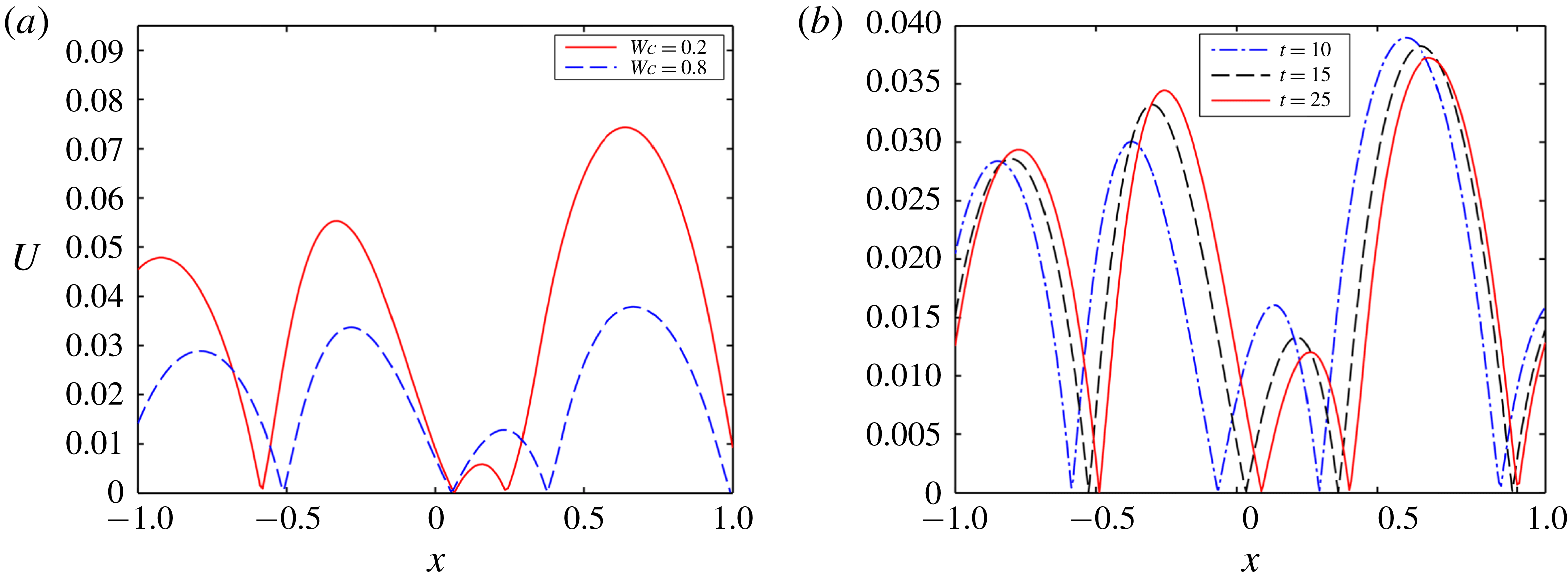
in both confined and unbounded domains. Figure 16(a) displays the fact that the inner droplet undergoes a to-and-fro motion for a weakly confined droplet. However, this to-and-fro motion surprisingly vanishes in a highly confined domain and the inner droplet moves towards the west pole of the outer droplet at comparatively lower speed. For the present system, the magnitude of
 $E^{2}$
is higher at the left side of the inner droplet as compared to the right side and the magnitude is also greater inside the inner droplet compared to the annular region, as shown in figure 16(b).
(a) Effect of confinement on the temporal variation of the position of the inner droplet for system III, (b) variation of
 $E^{2}$
along a straight horizontal line passing through the centre of the droplets from west pole to east pole of the outer droplet at
 $t=10$
, (c) streamline pattern of fluid flow circulation at
 $Wc=0.2$
, and (d) temporal variation of magnitude of velocity along a straight line passing through the centre from west pole to east pole of the droplet. Other parameters are
 $Ca_{E}=0.20$
,
 $(S_{23},R_{23})=(2,0.5)$
,
 $(S_{12},R_{12})=(0.5,2),Re=0.01$
,
 $e=0.25$
and
 $\unicode[STIX]{x1D706}=1$
.

Hence, the dielectrophoretic force pushes the inner droplet towards the west pole of the outer droplet. However, for the values of
 $R$
and
 $S$
 $(S_{12}<R_{12})$
used, the inner droplet undergoes a prolate deformation and the fluid flow occurs from equator to pole of the inner droplet, as shown in figure 16(c). Therefore, the EHD force at the west pole tries to push the droplet towards the east pole. On the contrary, the EHD force at the east pole tries to push the inner droplet in the opposite direction. Initially
 $(t=1)$
, the strength of fluid flow circulation is high at the left of the inner droplet, as can be seen from figure 16(d). Therefore, the net EHD force initially acts in the opposite direction to the dielectrophoretic force and drives the droplet towards the east pole of the outer droplet. Owing to the movement of the inner droplet towards the east pole of the outer droplet, the gap between the inner droplet and outer droplet reduces. This results in an increase in the film pressure at the reduced gap, which further creates a repulsive force that forces the inner droplet towards the west pole of the outer droplet. Furthermore, at this time
 $(t=10)$
, figure 16(d) shows that the magnitude of the velocity is also higher at the right side of the inner droplet. This signifies that the magnitude of the EHD force is also high at that side and the net EHD force acts towards the west pole of the outer droplet. The higher magnitude of the net EHD force along with the dielectrophoretic force are the main factors behind the motion of the droplet towards the west pole of the outer droplet. When the gap between the inner and outer droplet increases sufficiently
 $(t=25)$
, the magnitude of velocity again increases at the left side of the droplet, which is clearly understood from figure 16(d). Hence the net EHD force again acts opposite to the dielectrophoretic force and pushes the inner droplet towards the east pole of the outer droplet. This interplay among the repulsive force due to the interface of the outer droplet, the net EHD force and the dielectrophoretic force creates a to-and-fro motion of the inner droplet. Figures 16(b) and 17(a) show that the magnitudes of
 $E^{2}$
and the strength of fluid flow circulation are less in a confined domain, resulting in a reduced strength of the net dielectrophoretic force and EHD force, respectively. Furthermore, figure 17(b) shows that the magnitude of velocity is higher at the right side of the inner droplet throughout its motion. Hence, throughout the motion of the inner droplet, the net EHD force on it acts along the direction of the dielectrophoretic force. This creates a unidirectional translation motion of the inner droplet towards the west pole of the outer droplet. As the strengths of the net dielectrophoretic force and the EHD force are less in a confined domain, the motion of the inner droplet takes place very sluggishly.
(a) Effect of confinement on the magnitude of velocity along a horizontal straight line passing through the centre of the droplet from east pole to west pole, and (b) magnitude of velocity at different time intervals. Other parameters are
 $Ca_{E}=0.20$
,
 $Re=0.01$
,
 $e=0.25$
and
 $\unicode[STIX]{x1D706}=1$
.

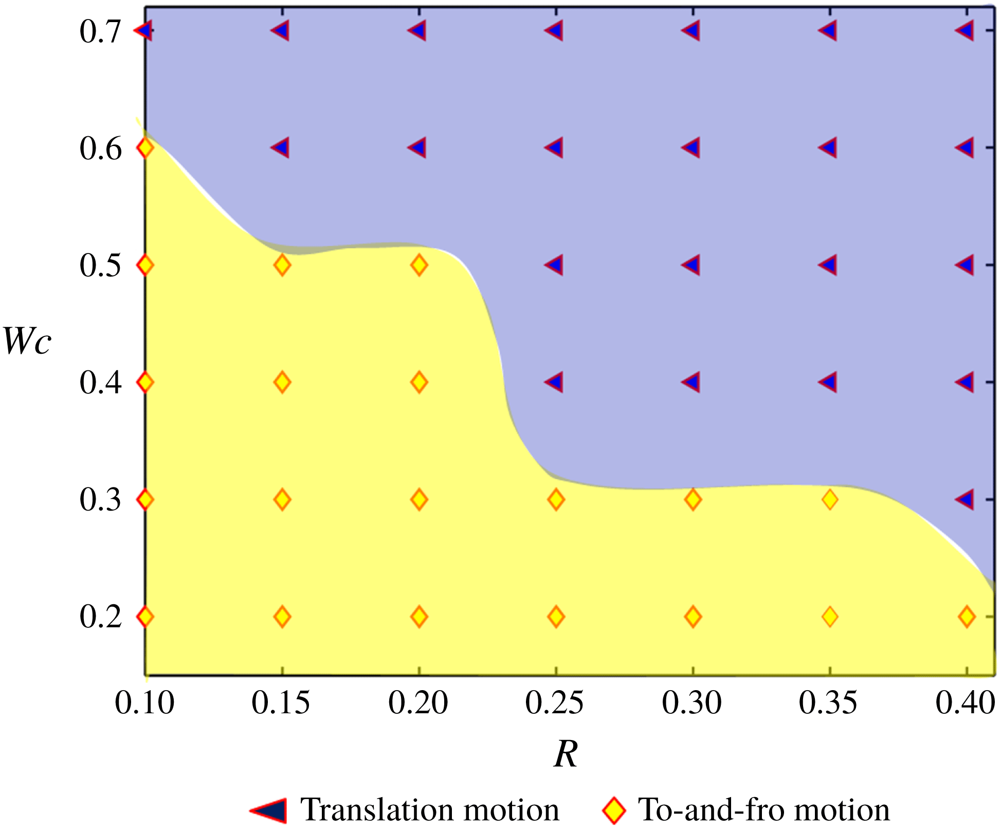
Next, we have formed a regime diagram that shows the pattern of the droplet motion based on the values of
 $(R,Wc)$
in figure 18. We have obtained two different patterns of inner droplet motion.
Regime plot showing the motion characteristics of the inner droplet. The different parameters are
 $(S_{23},S_{12})=(0.5,2)$
,
 $\unicode[STIX]{x1D706}=1$
,
 $Ca_{E}=0.2$
and
 $e=0.1$
. In the present plot, we have considered that
 $R_{23}=R=(R_{12})^{-1}$
.

The yellow-coloured region with diamond-shaped markers indicates that the droplet undergoes to-and-fro motion, whereas the blue-coloured regime with filled triangular-shaped markers signifies a unidirectional translational motion of the inner droplet towards the west pole of the outer droplet. Figure 18 also depicts that the conversion of droplet motion from to-and-fro to unidirectional translation motion occurs in a highly confined domain for lower values of the conductivity ratio
 $(R)$
. On the other hand, for relatively higher values of the conductivity ratio, the conversion of droplet motion takes place in a relatively weakly confined domain. As we mentioned earlier, the magnitude and direction of the EHD force on the inner droplet depends on the direction and strength of the EHD flow around the inner droplet. For the considered values of conductivity and permittivity ratio
 $(R_{12}>S_{12})$
, the EHD flow around the inner droplet takes place from the equator to the poles. Therefore, the EHD force at the right side of the inner droplet tries to move it towards the west pole of the outer droplet. On the contrary, the EHD force at the left side of the droplet tries to move the inner droplet towards the east pole of the outer droplet and the net EHD force finally determines the direction of the motion of the inner droplet. For the present case, the direction of the net EHD force is altered due to the change in confinement ratio and conductivity ratio of the system and plays a prime role in the conversion of droplet motion from to-and-fro motion to unidirectional translational motion.
3.4.2 Fluid system having different viscosities
In this section, the effect of viscosity ratio on the to-and-fro motion of the inner droplet in both a confined domain and an unbounded domain is shown. It is worth mentioning that the change in the dielectrophoretic force due to alteration of the viscosity ratio of the system is negligible. Therefore, the variation in the motion of the inner droplet occurs due to the sole effect of the net EHD force (refer to § 7 of the supplementary material for details). From figure 19(a), it can be inferred that the rate of droplet motion for LD–LD–LD system III with
 $(S_{23}>R_{23})$
and
 $(S_{12}<R_{12})$
is more at lower values of viscosity ratio
 $(\unicode[STIX]{x1D706}_{23})$
and the droplet undergoes to-and-fro motion.
(a) Effect of viscosity ratio on the temporal variation of the position of the inner droplet for system III with
 $(S_{23},R_{23})=(2,0.5)$
and
 $(S_{12},R_{12})=(0.5,2)$
, (b) effect of viscosity ratio on the variation of magnitude of velocity along a straight line passing through the centre from west pole to east pole of the droplet at
 $t=8$
and (c) effect of viscosity ratio on the variation of magnitude of velocity along a straight line passing through the centre from west pole to east pole of the droplet at
 $t=20$
. Other parameters are
 $Ca_{E}=0.20$
,
 $Re=0.01$
,
 $Wc=0.2$
and
 $e=0.25$
.

On the contrary, the motion of the inner droplet attenuates with increase in the values of
 $\unicode[STIX]{x1D706}_{23}$
. Interestingly, the to-and-fro motion of the inner droplet vanishes at higher values of the viscosity ratio
 $(\unicode[STIX]{x1D706}_{23}=10)$
. Initially
 $(t=8)$
, the magnitude of the velocity at the right side of the inner droplet is significantly higher for
 $\unicode[STIX]{x1D706}_{23}=0.1$
, as shown in figure 19(b). Therefore, the magnitude of the net EHD force on the inner droplet is also high for lower values of viscosity ratio, which causes faster motion of the inner droplet. After some time has passed
 $(t=20)$
, the magnitude of velocity becomes higher at the left (east) side of the inner droplet for lower values of viscosity ratio, as shown in figure 19(c). Therefore, the net EHD force creates a translation motion of the inner droplet towards the east pole of the outer droplet. On the other hand, figure 19(c) shows that the magnitude of velocity remains higher at the right side of the droplet for greater values of viscosity ratio. Hence, the direction of motion also remains unaltered.
Next, figure 20(a) shows the effect of viscosity ratio on the translation motion of the inner droplet in a confined domain. Unlike an unbounded domain, the inner droplet always undergoes unidirectional translation motion in a confined domain for all considered values of
 $\unicode[STIX]{x1D706}_{23}$
. It is also worth mentioning that the velocity of the inner droplet is high for lower values of the viscosity ratio similar to an unbounded domain. This can be easily understood from figure 20(b). From this figure, two important things should be noted: (i) the magnitude of velocity is higher at the right side of the inner droplet, which causes translation motion of the inner droplet towards the west pole of the outer droplet; and (ii) the magnitude of velocity at the right side of the inner droplet is higher for lower values of viscosity ratio, which causes faster translation motion of the inner droplet.
(a) Effect of viscosity ratio on the temporal variation of the position of the inner droplet for system III with
 $(S_{23},R_{23})=(2,0.5)$
and
 $(S_{12},R_{12})=(0.5,2)$
, and (b) effect of viscosity ratio on the variation of magnitude of velocity along a straight line passing through the centre from west pole to east pole of the droplet at
 $t=15$
. Other parameters are
 $Ca_{E}=0.20$
,
 $Re=0.01$
,
 $e=0.25$
and
 $Wc=0.8$
.

4 Conclusions
In summary, we have attempted to bring out several non-intuitive features concerning the dynamics of compound droplets in a microconfined fluidic environment, under the combined consequences of an electric field as well as confinement-induced hydrodynamic interactions. This, in turn, leads to a new paradigm of controlling morphological evolutions of compound droplets in microfluidic environments. By extending this principle, one may modulate the shape adaptation of compound droplets at will, by patterning the microfluidic surface with functionalized electrodes and switching them on and off as desired, through the exploitation of a combined influence of confinement and electromechanics; this paradigm has hitherto remained unexplored.
From the present study, the following major conclusions can be drawn.
(1) Although, under favourable conditions, combinations of perfectly dielectric systems for all the phases leads to an augmented deformation with increase in confinement for single droplets, the deformation is somewhat arrested for a compound droplet with all other conditions remaining unaltered.
(2) For a model system in which all the constituent phases are leaky dielectrics, the deformation of the inner droplet always shows a monotonic dependence on the confinement ratio. On the contrary, the outer droplet not only shows a non-monotonic variation in deformation, but also shows that the necessary condition for prolate deformation of the outer droplet switches from the classical paradigm if the confinement ratio increases beyond a threshold value, the magnitude of which is more for a compound droplet as compared to a single droplet. For this compound system, the deformations of both the inner and outer droplets are less when the viscosity of the suspending phase is greater compared to the annular phase. Another important point is that the threshold value of the domain confinement is also lower when the viscosity of the suspending medium is greater.
(3) In a highly confined domain, both the inner and the outer droplets attain steady-state configuration in a significantly more sluggish manner as compared to a single droplet that undergoes continuous elongation leading to an eventual breakup. Another important fact that needs to be noted is that, as compared to an equi-viscous system, the time required by both the outer and inner droplets to reach a steady-state configuration is longer when the viscosity of the suspending phase is less.
(4) In an unbounded domain, an eccentrically placed inner droplet of complete leaky dielectric system undergoes translational motion or to-and-fro migration, depending on the pertinent deformation parameters. Under extreme confinements, this dependence on the respective electrical parameters may be completely lost, and the inner droplet may undergo a rapid translation motion, bifurcating from the to-and-fro migratory regime. Furthermore, the viscosity contrast of the fluid phases also can induce or suppress the motion of the inner droplet (translational motion or to-and-fro migration), in both a confined and an unbounded domain.
The implications of the above reported observations may be far-reaching. For instance, embedded electrical chips may be designed to be located in physiological flow passages, in an effort to control the migratory characteristics and shape evolution of encapsulated cellular entities.
Acknowledgements
S.S. and S.D. are grateful to Dr S. Mandal for insightful discussions on droplet electrohydrodynamics. S.C. acknowledges the Department of Science and Technology, Government of India, for a Sir J. C. Bose National Fellowship.
Supplementary material
Supplementary material is available at https://doi.org/10.1017/jfm.2019.810. The supplementary material consists of two parts: a doc file (part 1) and a pdf file (part 2). The former comprises the asymptotic methodology, a grid independence study, domain confinement independence study, experimental relevance of assumptions and some detailed discussions based on the results presented here. The expressions for the coefficients encountered in the asymptotic analysis are too large to be provided in a doc file. Hence they are given in part 2 as an extract (.pdf file) from the MAPLE files.