



1. Introduction
The self-organised patterning in ultra-thin (
 $\lt$
100 nm) films has emerged as a crucial aspect of modern nanotechnology, underpinning a wide range of applications in sensors (Wang et al. Reference Wang, Rathi, Singh, Lee, Joh and Kim2015), microfluidic and microelectronic devices (Bhushan Reference Bhushan2007), self-cleaning surfaces (Koch et al. Reference Koch, Bhushan, Jung and Barthlott2009), textured coatings (Mayrhofer, Mitterer & Clemens Reference Mayrhofer, Mitterer and Clemens2005) and functional paints (Quére Reference Quéré1999), among others. These surface textures arise due to the instabilities in thin films that originate from intermolecular interactions (Van Oss, Chaudhury & Good Reference Van Oss, Chaudhury and Good1988; Reiter Reference Reiter1992; Sharma & Khanna Reference Sharma and Khanna1998; Chou, Zhuang & Guo Reference Chou, Zhuang and Guo1999; Seemann, Herminghaus & Jacobs Reference Seemann, Herminghaus and Jacobs2001), surface tension gradients (Cachile et al. Reference Cachile, Schneemilch, Hamraoui and Cazabat2002), wettability variations at the interfaces (Kumar & Whitesides Reference Kumar and Whitesides1994; Gau et al. Reference Gau, Herminghaus, Lenz and Lipowsky1999; Rockford et al. Reference Rockford, Liu, Mansky, Russell, Yoon and Mochrie1999; Konnur, Kargupta & Sharma Reference Konnur, Kargupta and Sharma2000; Kargupta & Sharma Reference Kargupta and Sharma2001) and the presence of surface defects (Jacobs, Herminghaus & Mecke Reference Jacobs, Herminghaus and Mecke1998; Verma & Sharma Reference Verma and Sharma2007). In addition to these intrinsic factors, externally applied fields such as electric and magnetic fields can also drive pattern formation (Dickstein et al. Reference Dickstein, Erramilli, Goldstein, Jackson and Langer1993; Schäffer et al. Reference Schäffer, Thurn-Albrecht, Russell and Steiner2000, Reference Schäffer, Thurn-Albrecht, Russell and Steiner2001; Morariu et al. Reference Morariu, Voicu, Schäffer, Lin, Russell and Steiner2003; Verma et al. Reference Verma, Sharma, Kargupta and Bhaumik2005; Chen & Li Reference Chen and Li2010; Seric, Afkhami & Kondic Reference Seric, Afkhami and Kondic2014). Compared with flat surfaces, nano/micro-patterned films offer distinct advantages, including enhanced transport processes, stronger intermolecular interactions and unique optical, mechanical and electronic properties at the nano and microscales. These attributes, arising from an increased surface-to-volume ratio, play a pivotal role in optimising the performance of advanced micro-nano-textured-based technologies.
Several top-down (Xia & Whitesides Reference Xia and Whitesides1998; Chou et al. Reference Chou, Zhuang and Guo1999) and bottom-up (Lu & Lieber Reference Lu and Lieber2007) approaches have been employed to pattern the soft surfaces of polymeric films. Among these, lithographically induced self-assembly (LISA) of a confined polymer layer has played a pivotal role in advancing our understanding of surface patterning. Experimental studies on LISA (Chou et al. Reference Chou, Zhuang and Guo1999; Deshpande, Sun & Chou Reference Deshpande, Sun and Chou2001; Cavallini & Biscarini Reference Cavallini and Biscarini2003), where pattern formation is driven by contact instability between the substrate and the polymer–air interface, laid the foundation for this field. These experimental insights were later supported by a detailed theoretical framework (Verma et al. Reference Verma, Sharma, Banerjee and Kargupta2006), which elucidated the underlying mechanisms of self-assembly. Additionally, the development of elastic contact lithography (ECL) introduced a new paradigm in surface patterning by enabling controlled adhesion and debonding, leading to improved tunability of aspect ratios in the resulting morphologies (Ghatak & Chaudhury Reference Ghatak and Chaudhury2003; Sarkar, Shenoy & Sharma Reference Sarkar, Shenoy and Sharma2004; Ghosh, Bandyopadhyay & Sharma Reference Ghosh, Bandyopadhyay and Sharma2016). The success of ECL has been demonstrated through various experimental advancements (Bietsch & Michel Reference Bietsch and Michel2000; Odom et al. Reference Odom, Love, Wolfe, Paul and Whitesides2002; Suh & Lee Reference Suh and Lee2002; Ghatak et al. Reference Ghatak, Mahadevan, Chung, Chaudhury and Shenoy2004; Gonuguntla et al. Reference Gonuguntla, Sharma, Sarkar, Subramanian, Ghosh and Shenoy2006; Mukherjee & Sharma Reference Mukherjee and Sharma2012; Bhandaru, Sharma & Mukherjee Reference Bhandaru, Sharma and Mukherjee2017), showcasing its potential for designing high-precision micro and nanoscale structures.
Electrohydrodynamic (EHD) instabilities in confined thin films have emerged as a promising approach to overcome the fundamental limitations associated with contact instabilities at relatively small separation distances between the deformable film surface and the contactor, thereby improving the aspect ratios of the self-organised patterns and enabling precise control over pattern densities. By remotely modulating destabilising fields, EHD-driven mechanisms allow tuneable periodicity in surface patterns. Early pioneering experiments by Schäffer et al. (Reference Schäffer, Thurn-Albrecht, Russell and Steiner2000, Reference Schäffer, Thurn-Albrecht, Russell and Steiner2001) demonstrated that an externally applied electrostatic field induces Maxwell stresses at the free surface of a soft dielectric polymeric film that can overcome stabilising capillary forces to form well-defined columnar structures. Building upon these findings, researchers refined EHD-driven patterning by incorporating templating techniques also termed as electric field lithography (EFL), where periodic physical and chemical patterns on bounding electrodes guided the formation of microstructures (Morariu et al. Reference Morariu, Voicu, Schäffer, Lin, Russell and Steiner2003; Verma et al. Reference Verma, Sharma, Kargupta and Bhaumik2005; Harkema & Steiner Reference Harkema and Steiner2005; Wu, Pease & Russel Reference Wu, Pease and Russel2005; Dickey et al. Reference Dickey, Gupta, Leach, Collister, Willson and Russell2006, Reference Dickey, Raines, Collister, Bonnecaze, Sreenivasan and Willson2008; Arun et al. Reference Arun, Sharma, Pattader, Banerjee, Dixit and Narayan2009; Goldberg-Oppenheimer & Steiner Reference Goldberg-Oppenheimer and Steiner2010; Srivastava et al. Reference Srivastava, Reddy, Wang, Bandyopadhyay and Sharma2010; Pattader et al. Reference Pattader, Banerjee, Sharma and Bandyopadhyay2011).
The periodicity of EHD-induced patterns is dictated by the mode of instability, which depends on the material properties of the thin film. Dielectric polymer films exhibit non-oscillatory long-wave instabilities, where a destabilising electric field induces surface deformations, while shorter wavelengths are stabilised by surface tension (Schäffer et al. Reference Schäffer, Thurn-Albrecht, Russell and Steiner2001; Verma et al. Reference Verma, Sharma, Kargupta and Bhaumik2005). Hookean films, in contrast, deform under a critical EHD field strength, destabilising intermediate wavelengths while elasticity and surface tension stabilise longer and shorter ones, respectively (Arun et al. Reference Arun, Sharma, Pattader, Banerjee, Dixit and Narayan2009). Leaky dielectric media further reduce pattern periodicity due to free charge accumulation at the film surface (Pease & Russel Reference Pease and Russel2004; Craster & Matar Reference Craster and Matar2005; Pease & Russel Reference Pease and Russel2006; Mondal, Kumar & Bandyopadhyay Reference Mondal, Kumar and Bandyopadhyay2013). Beyond material properties, the applied field also influences morphology. Switching from DC to AC fields alters the patterning dynamics (Roberts & Kumar Reference Roberts and Kumar2009), while extending ECL with an electric field (EFL) enhances aspect ratios, refining surface structures (Wang et al. Reference Wang, Rathi, Singh, Lee, Joh and Kim2015; Ghosh, Bandyopadhyay & Sharma Reference Ghosh, Bandyopadhyay and Sharma2018). For greater structural complexity, multi-layered films leverage combined contact and EHD instabilities to fabricate embedded, encapsulated and phase-inverted structures with reduced periodicity (Lin et al. Reference Lin, Kerle, Russell, Schäffer and Steiner2002a , Reference Lin, Kerle, Russell, Schäffer and Steinerb ; Merkt et al. Reference Merkt, Pototsky, Bestehorn and Thiele2005; Mukherjee et al. Reference Mukherjee, Pangule, Sharma and Tomar2007; Tomar et al. Reference Tomar, Sharma, Shenoy and Biswas2007; Bandyopadhyay et al. Reference Bandyopadhyay, Sharma, Thiele and Reddy2009; Roberts & Kumar Reference Roberts and Kumar2010; Reddy, Bandyopadhyay & Sharma Reference Reddy, Bandyopadhyay and Sharma2012). These advancements highlight the potential of EHD-driven patterning as a scalable and tuneable approach for engineering intricate multi-scale large-area architectures.
The studies discussed so far primarily focus on isotropic polymeric films. However, increasing attention has been directed towards instability-driven pattern formation in anisotropic materials, where the intrinsic anisotropy introduces additional complexity to the resulting morphologies and expands their potential applications (Ohm, Brehmer & Zentel Reference Ohm, Brehmer and Zentel2010; Jeong et al. Reference Jeong, Kim, Lee, Kim, Srinivasarao and Jung2012; Iino, Usui & Hanna Reference Iino, Usui and Hanna2015; Peng et al. Reference Peng, Guo, Turiv, Jiang, Wei and Lavrentovich2017). This added complexity also brings a unique challenge in the form of molecular orientational anisotropy on the elasticity of such films. In anisotropic materials like nematic liquid crystals (NLCs), the orientational order is typically described by a director field, representing the macroscopic average of the molecular alignment along their long axis (Chandrasekhar Reference Chandrasekhar1992; de Gennes & Prost Reference de Gennes and Prost1993). Due to elastic constraints in their self-organisation, most pattern-formation studies in NLC thin films have been restricted to investigations of phase transitions (Herminghaus et al. Reference Herminghaus, Jacobs, Mecke, Bischof, Fery, Ibn-Elhaj and Schlagowski1998; Vandenbrouck, Valignat & Cazabat Reference Vandenbrouck, Valignat and Cazabat1999; Van Effenterre et al. Reference Van Effenterre, Ober, Valignat and Cazabat2001; Ziherl & Zumer Reference Ziherl and Zumer2003; Ewiss et al. Reference Ewiss, Nabil, Schlagowski and Herminghaus2004; Garcia, Subashi & Fukuto Reference Garcia, Subashi and Fukuto2008) and contact instabilities in liquid crystal droplets (Poulard & Cazabat Reference Poulard and Cazabat2005; Delabre, Richard & Cazabat Reference Delabre, Richard and Cazabat2009; Manyuhina, Cazabat & Ben Amar Reference Manyuhina, Cazabat and Ben Amar2010; Rey & Herrera-Valencia Reference Rey and Herrera-Valencia2014; Ravi et al. Reference Ravi, Bhattacharjee, Ghosh and Bandyopadhyay2019; Thakur, Dasmahapatra & Bandyopadhyay Reference Thakur, Dasmahapatra and Bandyopadhyay2021). The latter was further supported by theoretical models (Lam et al. Reference Lam, Cummings and Kondic2018, Reference Lam, Kondic and Cummings2020), demonstrating pattern formation in confined NLC films. Beyond these approaches, solvent evaporation techniques have also been explored to achieve self-organised NLC morphologies. Studies indicate that diverse patterning modes can be realised when NLC concentration remains below a critical threshold (Ravi, Mukherjee & Bandyopadhyay Reference Ravi, Mukherjee and Bandyopadhyay2015; Dhara et al. Reference Dhara, Bhandaru, Das and Mukherjee2018; Dhara & Mukherjee Reference Dhara and Mukherjee2019; Ravi et al. Reference Ravi, Bhattacharjee, Ghosh and Bandyopadhyay2019; Chowdhury, Bhandary & Ghosh Reference Chowdhury, Bhandary and Ghosh2026). However, these morphologies lack precise control, and the underlying physics governing their formation remains an open question.
Beyond spontaneous instabilities, external-field-induced deformations in thin NLC films have enabled controlled morphology formation. Early studies demonstrated that the interplay between stabilising surface tension and gravitational forces and destabilising Ericksen stresses induced by an external magnetic field could deform macroscopic NLC film surfaces into hill-and-valley-like structures (Faetti & Palleschi Reference Faetti and Palleschi1985; de Gennes & Prost Reference de Gennes and Prost1993). Similar structures were later observed under an AC electric field applied perpendicular to the nematic–air interface, emerging beyond a critical field strength (Yokoyama, Kobayashi & Kamei Reference Yokoyama, Kobayashi and Kamei1985; Oswald Reference Oswald2010a , Reference Oswaldb ). Theoretical analyses further elucidated these external-field-driven instabilities. Studies on electric-field-induced deformations provided analytical insights into the observed surface modulations (Chandrasekhar Reference Chandrasekhar1992; de Gennes & Prost Reference de Gennes and Prost1993), while investigations on magnetic-field-driven instabilities at the nematic–air interface offered explanations for experimental patterns (Yokoyama Reference Yokoyama1988; Raghunathan Reference Raghunathan1995). These findings collectively established the role of external fields in manipulating the morphology of NLC films, paving the way for precise control over self-assembled structures.
While stability analyses and self-organisation studies of thin NLC films exist, a significant gap remains in our understanding of the morphological surface features that emerge when an external electric field is applied perpendicular to a free deformable NLC surface. In recent studies, Mondal et al. (Reference Mondal, Ghosh, Chaudhuri and Bandyopadhyay2018) investigated the stability of confined NLC films between two electrodes and identified the potentials for pattern formation across multiple length scales revealed by the coexistence of distinct finite and long-wave instability modes. This behaviour was driven by the interplay of key parameters, including electric field strength, air-to-NLC filling ratio, Frank elasticity, director orientation at the boundaries (Ericksen stresses) and dielectric anisotropy. A subsequent study by Mema, Kondic & Cummings (Reference Mema, Kondic and Cummings2021) examined the spatio-temporal evolution of an NLC film under a spatially varying electric field parallel to the deformable free surface, demonstrating a range of wrinkling patterns, such as non-sinusoidal, near sinusoidal, plateau–valley and multi-peak plateau, depending on electrode periodicity, filling ratio and surface anchoring. However, even spatially homogeneous electric fields in the perpendicular direction, as predicted by Mondal
 $et$
 $al.$
(Reference Mondal, Ghosh, Chaudhuri and Bandyopadhyay2018), suggested the formation of multi-scale morphologies, underscoring the potential of a one-step self-organisation process for fabricating hierarchical patterns. This highlights the need for further investigation into the dynamic interplay of anisotropic Maxwell and Ericksen stresses, air-to-NLC filling ratio, etc., which may hold the key to unlocking new pathways for controlled NLC patterning. Additionally, the fundamental molecular-level understandings on EHD instabilities engendered in such systems, based on the material’s intrinsic response to the applied external field, is also necessary to quantify the directionality of controlled self-organisation in thin films composed complex fluids like NLC, complementing the continuum-scale-based predictions and experimental observations.
Schematic diagram of a thin NLC film deforming under the influence of an external electric field potential of
 $\psi$
. The mean and the local thicknesses of the NLC film are denoted by
 $h_0$
and
 $h(x,t)$
, respectively. The distance between the electrodes is
 $d$
, and an air gap is present between the top electrode and the free surface of the film. The NLC film consists of rod-like molecules with an average orientation governed by the unit vector, termed the director,
 $\boldsymbol{n}\:\{n_x = \sin \theta , n_z = \cos \theta \}$
. Here,
 $\theta$
is the angle that the director makes with the positive
 $z$
-axis.

Given these complexities, we systematically explore the interplay of key parameters, and the fundamental molecular-level mechanism that enable EHD-pattern formation in thin NLC films. Prior studies (Verma et al. Reference Verma, Sharma, Kargupta and Bhaumik2005; Pattader et al. Reference Pattader, Banerjee, Sharma and Bandyopadhyay2011) suggest that these interplays can lead to a diverse range of multi-scale, uniform and coalesced morphologies in a thin isotropic liquid, or polymeric films by means of EHD instability, but a comprehensive understanding on analogous EHD patterning in their anisotropic counterparts remains largely unresolved. To address this, we employ a multi-scale approach in this study to:
-
(i) explore the salient morphological features of the electrostatically sandwiched NLC films bounded by air, as shown in figure 1, using the developed nemato–EHD thin-film evolution equation and employing nonlinear simulations (NS) aided by long-wave linear stability analysis (LWLSA);
-
(ii) provide a detailed picture of the director (molecular) orientation and the fundamental thermodynamic perspective on EHD-instability-driven pattern formation in thin NLC films using molecular dynamics (MD) simulations;
-
(iii) compare the molecular orientation profile within the morphologies computed from NS with MD predictions, to demonstrate the potential applicability of the resulting morphologies with distinct molecular orientations in nano-microfabrication techniques, like photolithography (Roscioni et al. Reference Roscioni, Muccioli, Della Valle, Pizzirusso, Ricci and Zannoni2013, Reference Roscioni, Muccioli and Zannoni2017; Thakur et al. Reference Thakur, Dasmahapatra and Bandyopadhyay2021; Liu et al. Reference Liu, Yang, Guo, Chen, Feng, Lu, Huang, Zhang, Ye and Shui2024).
To systematically evaluate the effect of boundary conditions, we investigate director-field solutions under different strong anchoring conditions
 $-$
homeotropic, angular and planar
 $-$
at the nematic–solid interface to determine their influence on the resulting morphology. Meanwhile, at the nematic–air free interface, predominantly a homeotropic anchoring is exhibited due to the orientation of NLC molecules in the direction of applied electric field. The proposed self-organisation of NLC films leads to the formation of secondary multi-scale structures, that become more prominent with increasing anisotropy at lower NLC-to-air filling ratios, exhibiting an aspect ratio of
 $\sim$
6, while the primary uniform columnar-like structures can achieve an aspect ratio exceeding
 $\sim$
12 without undergoing coalescence. Additionally, surface anchoring at the nematic–solid interface can be tuned to ‘arrest’ coalescence, which has critical implications for ‘clean’ peeling in pressure-sensitive adhesive applications. The qualitative agreements between the molecular-scale and continuum-scale predictions in resulting morphological outcomes, despite the inherent disparity in length/time scales, warranted a comprehensive parametric analysis in seeking pathways to on-demand morphological patterns of NLC. Furthermore, our director-field solutions suggest that primary structures could serve as ‘photomasks’ in photolithographic applications. To broaden the applicability of these findings, the pathways for miniaturised multi-scale structures with varying aspect ratios and tapered geometries have been unveiled, providing potential applications in superhydrophobic surfaces and biomimetic prototypes that exploit anisotropic and multi-stimuli-sensitive properties.
The article is arranged in the following manner. Sections 2 and 3 contain the details of the continuum-scale and molecular-scale methodologies to model the system of interest, respectively. Section 4 presents the discussions of the results obtained, which are initiated with molecular-scale observations, establishing the principal modes governing EHD patterning with details on director profiles, followed by continuum-scale observations that validate the findings against previous studies and further explore the morphological transitions in greater detail over larger accessible length and time scales. Finally, the conclusions drawn from this study are presented in § 5.
2. Continuum model: theoretical formulation and numerical methodologies
2.1. Equations of nemato-electrohydrodynamics
We adopt a two-dimensional Cartesian coordinate system in this study, with the origin located at the NLC–substrate (bottom electrode) interface, as shown in figure 1. The NLC film, characterised by an instantaneous thickness
 $h(x,t)$
with an average value
 $h_0$
, is confined between two electrodes separated by a distance
 $d$
. The film considered in the present study is thin enough to be characterised as a low Reynolds number system, to neglect the inertial forces. Also, the magnitude of the electric field is considered much stronger than that of gravity. The dynamics of such an incompressible, isothermal and dielectric thin NLC film in the presence of an applied electric field can be expressed using the Ericksen–Leslie governing equations of nematodynamics (Ericksen Reference Ericksen1962; Leslie Reference Leslie1992; Chandrasekhar Reference Chandrasekhar1992; Ben Amar & Cummings Reference Ben Amar and Cummings2001; Cummings Reference Cummings2004; Stewart Reference Stewart2004; Mondal et al. Reference Mondal, Ghosh, Chaudhuri and Bandyopadhyay2018; Mema et al. Reference Mema, Kondic and Cummings2021) as
 \begin{align} \boldsymbol{n}\boldsymbol{\cdot }\boldsymbol{n}&=1, \end{align}
 \begin{align} \boldsymbol{\boldsymbol{\nabla }\boldsymbol{\cdot }\boldsymbol{u}}&=0, \end{align}
 \begin{align} \boldsymbol{\nabla }\boldsymbol{\cdot }(-p\boldsymbol{I}+{\boldsymbol{\unicode {x03C0}}}_{\textit{Er}})+\boldsymbol{\nabla }\boldsymbol{\cdot }(\boldsymbol{\unicode {x03C4}}+\boldsymbol{M})&=0, \end{align}
 \begin{align} \lambda \boldsymbol{n}-\frac {\partial F}{\partial \boldsymbol{n}}+\boldsymbol{\nabla }\boldsymbol{\cdot }\bigg (\frac {\partial F}{\partial \boldsymbol{\nabla }\boldsymbol{n}}\bigg )+\boldsymbol{G}+\boldsymbol{g}&=0. \end{align}
Equation (2.1) represents the constraint imposed on the director field, which is further ensured by a Lagrange multiplier
 $\lambda$
in (2.4) (Tavener et al. Reference Tavener, Mullin, Blake and Cliffe2000). In a two-dimensional Cartesian coordinate system the director vector
 $\boldsymbol{n}$
can be expressed as
 $\boldsymbol{n}\{n_x, n_z\}$
, where
 $n_x=\sin \theta , n_z=\cos \theta$
, satisfying (2.1), where
 $\theta$
is the anchoring angle, i.e. angle the director makes with the positive
 $z$
-axis. The other notations
 $\boldsymbol{u}\{u,v\}$
,
 $\boldsymbol{\unicode {x03C0}}_{\textit{Er}}$
,
 $\boldsymbol{M}$
,
 $\boldsymbol{\unicode {x03C4}}$
,
 $p$
,
 $\boldsymbol{I}$
and
 $\boldsymbol{\nabla}$
stand for velocity vector, Ericksen elastic stress tensor, Maxwell stress tensor due to the electric field, deviatoric stress tensor for the flow field, hydrostatic pressure, identity matrix and the gradient operator, respectively; curly bracketed symbols denote the vector components. The variables in these equations, like Frank free energy (
 $F$
), the external director body force due to electric field (
 $\boldsymbol{G}$
) and the intrinsic director body force (
 $\boldsymbol{g}$
), are defined as (Chandrasekhar Reference Chandrasekhar1992)
 \begin{align} F&=\frac {1}{2}k_{11}\big (\boldsymbol{\nabla }\boldsymbol{\cdot }\boldsymbol{n}\big )^2+ \frac {1}{2}k_{22}\big (\boldsymbol{n}\boldsymbol{\cdot }\boldsymbol{\nabla }\times \boldsymbol{n}\big)^2 +\frac {1}{2}k_{33}\big (\boldsymbol{n}\times \boldsymbol{\nabla }\times \boldsymbol{n}\big)^2\notag\\&\quad + \frac {1}{2}\big(k_{22}+k_{44}\big)\boldsymbol{\nabla }\boldsymbol{\cdot }\big [(\boldsymbol{n}\boldsymbol{\cdot }\boldsymbol{\boldsymbol{\nabla }})\boldsymbol{n}-(\boldsymbol{\nabla }\boldsymbol{\cdot }\boldsymbol{n})\boldsymbol{n}\big ], \end{align}
 \begin{align} \boldsymbol{G}&=\varepsilon _0\varepsilon _d(\boldsymbol{E\boldsymbol{\cdot }n})\boldsymbol{E}, \end{align}
 \begin{align} \boldsymbol{g}&=-\lambda _1\boldsymbol{N}-\lambda _2(\boldsymbol{e \boldsymbol{\cdot }n}). \end{align}
The parameter
 $\varepsilon _d (=\varepsilon _{\parallel }-\varepsilon _{\perp } )$
is the dielectric anisotropy, and
 $\varepsilon _{\parallel }$
(
 $\varepsilon _{\perp }$
) is the dielectric constant of the NLC film measured parallel (perpendicular) to its director (de Gennes & Prost Reference de Gennes and Prost1993). Additionally,
 $\varepsilon _0$
and
 $\varepsilon _a$
refer to the dielectric permittivity of vacuum and air, respectively. The variables
 $k_{11}, k_{22}, k_{33},$
and
 $(k_{22} + k_{24})$
are the splay, twist, bend and saddle-splay elastic constants, respectively. Equation (2.5) reduces to a simpler form,
 $F=0.5k_f [(\boldsymbol{\nabla }\boldsymbol{\cdot }\boldsymbol{n})^2+|\boldsymbol{\nabla }\times \boldsymbol{n}|^2 ]$
, in the limit of one constant approximation,
 $k_{11}=k_{22}=k_{33}=k_f$
, where
 $k_f$
stands for the bulk elastic constant of the thin NLC film (de Gennes & Prost Reference de Gennes and Prost1993). On the other hand, the terms contributing to the saddle splay vanishes in the limit of two-dimensional analysis. In (2.7) the linear deformation tensor is defined as
 $\boldsymbol{e}=(\boldsymbol{\nabla }\boldsymbol{u}+\boldsymbol{\nabla }\boldsymbol{u^{\mathrm{T}}})/2$
, the rotation vector is defined as
 $\boldsymbol{N}=\dot {\boldsymbol{n}}-\boldsymbol{\omega \boldsymbol{\cdot }\boldsymbol{n}}$
and the spin tensor is defined as
 $\boldsymbol{\omega }=(\boldsymbol{\nabla }\boldsymbol{u}-\boldsymbol{\nabla }\boldsymbol{u^{\mathrm{T}}})/2$
. The Ericksen elastic stress tensor,
 $\boldsymbol{\pi }_{\textit{Er}}$
, is defined as
 \begin{equation} \boldsymbol{\pi }_{\textit{Er}} = -\bigg (\frac {\partial F}{\partial \boldsymbol{\nabla }\boldsymbol{n}}\bigg )\boldsymbol{\cdot }(\boldsymbol{\nabla }\boldsymbol{n})^{\mathrm{T}}. \end{equation}
The deviatoric stress tensor for the thin NLC film is defined as (Chandrasekhar Reference Chandrasekhar1992; Leslie Reference Leslie1992)
 \begin{equation} \boldsymbol{\unicode {x03C4}} = \alpha _1\boldsymbol{e}:\boldsymbol{nnnn} + \alpha _2\boldsymbol{nN} + \alpha _3\boldsymbol{Nn} + \alpha _4\boldsymbol{e} + \alpha _5\boldsymbol{nn}:\boldsymbol{e} + \alpha _6\boldsymbol{e}:\boldsymbol{nn}, \end{equation}
where the
 $i^{\text{}}$
th Leslie viscosity coefficient is denoted by the symbol
 $\alpha _i$
. The rotational viscosity and the irrotational torque coefficient in (2.7) are defined as
 $\lambda _1=\alpha _3-\alpha _2$
and
 $\lambda _2=\alpha _6-\alpha _5$
. The sixth Leslie viscosity coefficient (
 $\alpha _6$
), is evaluated from the Onsager–Parodi relation,
 $\lambda _2=\alpha _6-\alpha _5=\alpha _2+\alpha _3$
(Stewart Reference Stewart2004; Mondal et al. Reference Mondal, Ghosh, Chaudhuri and Bandyopadhyay2018).
The Maxwell stresses due to the external electric field is defined as (Yokoyama et al. Reference Yokoyama, Kobayashi and Kamei1985)
 \begin{equation} \boldsymbol{M}=\boldsymbol{DE}-\frac {1}{2}(\boldsymbol{D \boldsymbol{\cdot }E})\boldsymbol{I}, \end{equation}
where the electric displacement field is defined as
 $\boldsymbol{D} = \varepsilon _0 [\varepsilon _{\perp }\boldsymbol{E} + \varepsilon _d(\boldsymbol{E\boldsymbol{\cdot }n})\boldsymbol{n}]$
, and the electric field is defined as
 $\boldsymbol{E}=-\boldsymbol{\nabla }\psi$
, where
 $\psi$
stands for the electric field potential. Further, the NLC film is considered to be non-conducting with a dielectric anisotropy originating from the difference in the dielectric constants in the directions parallel (
 $\varepsilon _{\parallel }$
) and normal (
 $\varepsilon _{\perp }$
) to the applied field. Thus, the governing equation of an irrotational electric field (
 $\boldsymbol{\nabla }\times \boldsymbol{E} = 0$
) for the NLC film can be written as
 \begin{equation} \boldsymbol{\nabla }\boldsymbol{\cdot }\boldsymbol{D} = 0. \end{equation}
The irrotational electric field potential for a purely dielectric air film (bounding film) can be expressed as
 \begin{equation} \boldsymbol{\nabla }\boldsymbol{\cdot }\boldsymbol{E}_a = \boldsymbol{\nabla} ^2\psi _a = 0. \end{equation}
2.2. Boundary conditions
Hydrodynamics
 $-$
the NLC film is assumed to be present on a no-slip, impermeable electrode located at
 $z=0$
, subjected to the boundary condition
 \begin{equation} \boldsymbol{u}=0. \end{equation}
At NLC–air interface (
 $z = h$
), the normal and the tangential stress balances together with the kinematic condition are enforced as
 \begin{align} \boldsymbol{n}_s\boldsymbol{\cdot }(-p_0\boldsymbol{I}+\boldsymbol{M}_a) \boldsymbol{\cdot }\boldsymbol{n}_s - \boldsymbol{n}_s\boldsymbol{\cdot }(-p_0\boldsymbol{I}+\boldsymbol{\unicode {x03C0}}_{\textit{Er}}+\boldsymbol{\unicode {x03C4}}+\boldsymbol{M}) \boldsymbol{\cdot }\boldsymbol{n}_s &= \gamma \kappa , \end{align}
 \begin{align} \boldsymbol{n}_s\boldsymbol{\cdot }\boldsymbol{M}_a \boldsymbol{\cdot }\boldsymbol{t}_s - \boldsymbol{n}_s\boldsymbol{\cdot }(\boldsymbol{\unicode {x03C0}}_{\textit{Er}}+\boldsymbol{\unicode {x03C4}}+\boldsymbol{M}) \boldsymbol{\cdot }\boldsymbol{t}_s &= 0, \end{align}
 \begin{align} \frac {\partial h}{\partial t}+\boldsymbol{u\boldsymbol{\cdot }\boldsymbol{\nabla} }_s h&=w. \end{align}
The subscript ‘a’ denotes the variables corresponding to the bounding fluid air. The variables
 $p_0, h, \gamma $
and
 $\kappa =-\boldsymbol{\nabla} _s\boldsymbol{\cdot }\boldsymbol{n}_s$
denote ambient air pressure, film thickness, surface tension of the film and the curvature of the deforming surface. The notations
 $\boldsymbol{\nabla} _s$
,
 $\boldsymbol{n}_s$
and
 $\boldsymbol{t}_s$
denote the surface gradient operator, unit outward normal and tangent vectors,
 $(\boldsymbol{I-nn})\boldsymbol{\cdot }\boldsymbol{\nabla}$
,
 $\boldsymbol{\nabla }(z-h)/\left |\boldsymbol{\nabla }(z-h)\right |$
and (1,
 $h_x$
)/
 $\sqrt {(1+h^2_x)}$
, respectively.
Director
 $-$
strong anchoring Dirichlet boundary condition of the director field is employed at the NLC–solid interface, since the orientation of NLC molecules can be physically tuned by surface functionalisation. Moreover, a strong anchoring condition is also imposed at the NLC–air interface at
 $z=h(x,t)$
. Since the electric field is applied perpendicular to the NLC–air interface, the director field spontaneously reorients parallel to the field direction, regardless of the anchoring energy at the free surface due to Fréedericksz transition (FT), as predicted by Mondal
 $et$
 $al.$
(Reference Mondal, Ghosh, Chaudhuri and Bandyopadhyay2018). Molecular dynamics simulations presented in this study provided a detailed justification for this approximation. The director field can exhibit typically three modes of anchoring at the NLC–solid (
 $z=0)$
, and NLC–air (
 $z=h$
) interfaces: (i) planar–homeotropic (
 $\theta _1 = 90^{\circ }, \theta _2=0^{\circ }$
), (ii) homeotropic–homeotropic (
 $\theta _1 = 0^{\circ }, \theta _2=0^{\circ }$
) and (iii) angular–homeotropic (
 $0^{\circ }\lt \theta _1\lt 90^{\circ }, \theta _2 = 0^{\circ }$
), where
 \begin{align} \theta (z=0) &= \theta _1, \end{align}
 \begin{align} \theta (z=h) &= \theta _2. \end{align}
Electrostatics
 $-$
constant electrostatic potential boundary conditions are enforced at
 $z=0$
and
 $z=d$
as
 \begin{align} \psi &= 0, \end{align}
 \begin{align} \psi _a &= \psi _0. \end{align}
The continuity in normal and the tangential component balances of the electric field across the NLC and bounding air film are also employed at
 $z=h(x,t)$
as
 \begin{align} \boldsymbol{D}_a\boldsymbol{\cdot }\boldsymbol{n}_s&=\boldsymbol{D}\boldsymbol{\cdot }\boldsymbol{n}_s, \end{align}
 \begin{align} \boldsymbol{E}_a\boldsymbol{\cdot }\boldsymbol{t}_s&=\boldsymbol{E}\boldsymbol{\cdot }\boldsymbol{t}_s. \end{align}
2.3. Non-dimensionalised equations
The dimensional governing equations and boundary conditions presented in the previous section are first converted to dimensionless forms with the help of the following scalings:
 \begin{align} (X,Z,H,D)&=\dfrac {(x,z,h,d)}{h_0} \text{; } T=t\bigg (\dfrac {\varepsilon _0\psi ^2_0}{2\mu h^2_0}\bigg ) \text{; } (U,W)=(u,w)\bigg (\dfrac {2\mu h_0}{\varepsilon _0\psi ^2_0}\bigg ) \text{, } \end{align}
 \begin{align} (P,P_0)&=(p,p_0)\bigg (\dfrac {2h_0}{\varepsilon _0\psi ^2_0}\bigg ) \text{; } \varLambda _i=\dfrac {\lambda _i}{\mu } \text{; and } (\varPsi ,\varPsi _a)=\dfrac {(\psi ,\psi _\textit{a})}{\psi _0} \text{ ,} \end{align}
where the equivalent Newtonian viscosity (
 $\mu =\alpha _4/2$
) is used for the scaling. Further, the equations are rescaled employing
 \begin{align} (\hat {X},\hat {Z})=(\delta X,Z) \text{ ; } (\hat {U}, \delta \hat {W})=\dfrac {(U,W)}{\delta } \text{ and } \hat {T}=\delta ^2 T \text{ , where } \delta =\sqrt {\dfrac {\varepsilon _0{\psi _0}^2}{2\gamma h_0}}. \end{align}
The rescaling is analogous to the lubrication approximation (Mondal et al. Reference Mondal, Ghosh, Chaudhuri and Bandyopadhyay2018) and performed to develop the coupled nemato–EHD thin-film evolution equation in the long-wave limit. To improve readability, the rescaled variables, originally denoted by hats, are presented without hats in the final equations.
2.3.1. Governing equations
The resulting continuity (2.2) can be written as
 \begin{equation} U_{,X}+W_{,Z} = 0. \end{equation}
The
 $X$
and
 $Z$
-components of the linear momentum balance (2.3) are
 \begin{align} P_{,X}&= B_2U_{,\textit{ZZ}}+\delta ^3 A_3W_{,\textit{XX}}-\delta ^2(A_1-A_4-B_3)W_{,\textit{ZX}}\notag\\ &\quad -\delta (A_2+B_1-B_4)W_{,\textit{ZZ}} +B_{2,Z}U_{,Z}+\delta ^2 B_{3,Z}W_{,X} -\delta (B_1-B_4)_{,Z}W_{,Z}\notag\\ &\quad -\frac {1}{2Er}{\theta ^2_{,Z}}_{,X} - \delta 2\varepsilon _d\cos 2\theta \varPsi _{a,X}\varPsi _{a,Z}\theta _{,X} -\bigg (\frac {1}{\textit{Er}}\theta _{,\textit{ZZ}}-\varepsilon _d\sin 2\theta {\varPsi ^2_{a,Z}}\bigg )\theta _{,X}, \end{align}
 \begin{align} P_{,Z} &= \delta D_2 U_{,\textit{ZZ}} + \delta ^4 C_3 W_{,\textit{XX}} - \delta ^3 (C_1-C_4-D_3)W_{,\textit{ZX}} - \delta ^2 (C_2+D_1-D_4)W_{,\textit{ZZ}} \notag\\&\quad +\delta D_{2,Z}U_{,Z}+ \delta ^3 D_{3,Z} W_{,X}- \delta ^2 (D_1-D_4)_{,Z}W_{,Z} - \frac {1}{2Er}{\theta ^2_{,Z}}_{,Z} - \frac {\delta ^2 }{\textit{Er}}\theta _{,\textit{XX}}\theta _{,Z} \notag\\&\quad -\delta 2\varepsilon _d\cos 2\theta \varPsi _{a,X}\varPsi _{a,Z}\theta _{,Z} - \bigg (\frac {1}{\textit{Er}}\theta _{,\textit{ZZ}}-\varepsilon _d\sin 2\theta \varPsi ^2_{a,Z}\bigg )\theta _{,Z}. \end{align}
In the above expressions, the subscripts (
 $X, Z$
or
 $T$
) separated by a comma from the variables denote partial differentiations with respect to the subscripted variables. The dimensionless Ericksen number
 ${\textit{Er}}=(({\varepsilon _0\psi ^2_0})/({2k_f}))$
signifies the ratio of the applied electrostatic force to the bulk elastic resistance of the NLC film. The expressions of the non-dimensional viscosity coefficients,
 $A_i, B_i, C_i$
and
 $D_i$
, are provided in Appendix A. The
 $X$
and
 $Z$
-components of angular momentum balance (2.4) are combined to obtain the following:
 \begin{align} &\frac {1}{\textit{Er}}(\delta ^2\theta _{,\textit{XX}}+\theta _{,\textit{ZZ}}) +2\varepsilon _d\bigg [\delta ^2 \varPsi ^2_{,X}\frac {\sin 2\theta }{2}+ \delta \cos 2\theta \varPsi _{,X}\varPsi _{,Z}-\varPsi ^2_{,Z}\frac {\sin 2\theta }{2} \bigg ]\notag\\&\quad +\frac {\delta }{2}\bigg [\varLambda _1(\delta ^2 W_{,X}-U_{,Z})+\varLambda _2(\delta ^2 W_{,X}+U_{,Z})\cos 2\theta - \delta 2\varLambda _2\sin 2\theta W_{,Z}\bigg ]=0. \end{align}
Rescaling the electrodynamic equations from (2.11) to (2.12) for the NLC film and air yielded
 \begin{align} &\varepsilon _{\perp }\big (\delta ^2\varPsi _{,\textit{XX}}+\varPsi _{,\textit{ZZ}}\big )+\varepsilon _d\sin 2\theta \big (\delta ^2 \theta _{,X}\varPsi _{,X}-\theta _{,Z}\varPsi _{,Z}\big )+\varepsilon _d\big (\delta ^2 \sin ^2\theta \varPsi _{,\textit{XX}} +\cos ^2\theta \varPsi _{,\textit{ZZ}}\big )\notag\\&\quad +\delta \cos 2\theta \big (\theta _{,X}\varPsi _{,Z} -\theta _{,Z}\varPsi _{,X}\big )+\delta \varepsilon _a\sin 2\theta \varPsi _{,\textit{ZX}}=0, \end{align}
 \begin{align}&\qquad\qquad\qquad\qquad\qquad\qquad \delta ^2\varPsi _{a,\textit{XX}}+\varPsi _{a,\textit{ZZ}}=0. \end{align}
2.3.2. Boundary conditions
The non-dimensional form of the no-slip and impermeability boundary conditions (2.13) at
 $Z=0$
become
 \begin{equation} U=W=0. \end{equation}
The director orientation boundary conditions (2.17) at the NLC–solid (
 $Z=0$
), and NLC–air (
 $Z=H$
) interfaces are
 \begin{align} \theta &= \theta _1, \end{align}
 \begin{align} \theta &= \theta _2. \end{align}
The boundary conditions for the electric field (2.18) at the bottom (
 $Z=0$
) and top contactors (
 $Z=D$
) are
 \begin{align} \varPsi =0, \end{align}
 \begin{align} \varPsi _a=1. \\[10pt] \nonumber \end{align}
The rescaled versions of the normal and tangential stress balances together with the kinematic condition (2.14)–(2.16) at
 $Z=H$
are obtained as
 \begin{align}&\quad P_M-P_0-\big(\delta ^2 D_1 U_{,X} + \delta D_2 U_{,Z} + \delta ^3 D_3 W_{,X}+D_4 \delta ^2 W_{,Z}\big) \notag\\&\qquad +\big[\varepsilon _d\big(\delta \sin 2\theta H_{,X}-\cos ^2\theta \big)-\varepsilon _{\perp }\big] \varPsi ^2_{,Z}+\varPsi ^2_{a,Z}=-H_{,\textit{XX}}-\frac {1}{2Er}\theta ^2_{,Z}, \end{align}
 \begin{align}& \frac {1}{\textit{Er}}\big(\delta \theta ^2_{,Z}H_{,X}+ \delta \theta _{,X}\theta _{,Z}\big) + \big(\delta ^2 B_1 U_{,X} + \delta B_2 U_{,Z} + \delta ^3 B_3 W_{,X} + \delta ^2 B_4 W_{,Z}\big)=0, \end{align}
 \begin{align}&\qquad\qquad\qquad\qquad\qquad\qquad H_{,T}+UH_{,X}=W. \end{align}
Here,
 $P_0$
stands for the non-dimensional pressure of ambient air,
 $P$
stands for the non-dimensional hydrostatic pressure of the NLC film and
 $P_M=P+({1}/({2Er}))\theta ^2_{,Z}$
.
The non-dimensional forms of the normal and tangential component balances (2.19) of the electric field at the NLC–air interface (
 $Z=H$
) are obtained as
 \begin{align}& \delta H_{,X}\bigg [\delta (\varepsilon _{\perp }+\varepsilon _{d}\sin ^2\theta ) \varPsi _{,X}+\varepsilon _d \frac {\sin 2\theta }{2}\varPsi _{,Z}\bigg ]-(\varepsilon _{\perp }+\varepsilon _{d}\cos ^2\theta )\varPsi _{,Z}\notag\\&\quad -\delta \varepsilon _a\frac {\sin 2\theta }{2}\varPsi _{,X} +\varepsilon _a\big (\varPsi _{a,Z}-\delta \varepsilon _a\varPsi _{a,X}\big )=0, \end{align}
 \begin{align}&\qquad\qquad\qquad \big (\varPsi _{a,X}-\varPsi _{,X}\big )+H_{,X}\big (\varPsi _{a,Z}-\varPsi _{,Z}\big )=0. \end{align}
2.4. Nonlinear nemato-electrohydrodynamic thin-film evolution equation
The leading-order terms of the re-scaled non-dimensional equations ((2.23)–(2.36)) are retained to derive the free thin NLC film evolution equation (Ben Amar & Cummings Reference Ben Amar and Cummings2001; Cummings Reference Cummings2004; Mondal et al. Reference Mondal, Ghosh, Chaudhuri and Bandyopadhyay2018; Mema et al. Reference Mema, Kondic and Cummings2021).
2.4.1. Governing equations
The long-wave, non-dimensional
 $X$
and
 $Z$
-components of the equations of motion (2.24)–(2.25), angular momentum balance (2.26) and electric field potential for the NLC film and air (2.27)–(2.28) are
 \begin{align} P_{M,X}&=\big (B_2U_{,Z}\big )_{,Z}, \end{align}
 \begin{align} P_{M,Z}&=0, \end{align}
 \begin{align} \dfrac {1}{\textit{Er}}\theta _{,\textit{ZZ}}&=0, \end{align}
 \begin{align} \big [\big(\varepsilon _{\perp }+\varepsilon _d\cos ^2\theta \big)\varPsi _{,Z}\big ]_{,Z}&=0, \end{align}
 \begin{align} \varPsi _{a,\textit{ZZ}}&=0. \end{align}
2.4.2. Boundary conditions
The no-slip and impermeable boundary conditions (2.29) for the velocity field turn out at the NLC–solid interface (
 $Z=0$
) as
 \begin{equation} U=W=0. \end{equation}
The director orientation boundary conditions (2.30) at the NLC–solid (
 $Z=0$
), and NLC–air (
 $Z=H$
) interfaces are
 \begin{align} \theta &= \theta _1, \end{align}
 \begin{align} \theta &= \theta _2. \\[10pt] \nonumber \end{align}
The boundary conditions for the electric field (2.31) at the bottom (
 $Z=0$
) and top contactors (
 $Z=D$
) are
 \begin{align} \varPsi =0, \end{align}
 \begin{align} \varPsi _a=1. \end{align}
The reduced long-wave kinematic condition, normal and tangential stress balances and the balances of normal and tangential components of the electric field at the NLC–air interface (
 $Z=H$
) are
 \begin{align} H_{,T}+U_{,Z}H_{,X}&=W_{,Z},\end{align}
 \begin{align} P_{M}&=P_0-H_{,\textit{XX}}-\frac {1}{2Er}\theta ^2_{,Z}+\big(\varepsilon _{\perp }+\varepsilon _d\cos ^2\theta \big)\varPsi ^2_{,Z}-\varPsi ^2_{a,Z},\end{align}
 \begin{align} U_{,Z}&=0,\end{align}
 \begin{align} \big(\varepsilon _{\perp }+ \varepsilon _d\cos ^2\theta \big)\varPsi _{,Z}&=\varepsilon _a\varPsi _{a,Z},\end{align}
 \begin{align} \varPsi &=\varPsi _a.\end{align}
The kinematic (2.45) is expressed in the above form using the relation
 $\int _0^H U\,\text{d}Z=\int _0^H U_{,Z}(H-Z)\,\text{d}Z$
(Ben Amar & Cummings Reference Ben Amar and Cummings2001; Cummings Reference Cummings2004; Mondal et al. Reference Mondal, Ghosh, Chaudhuri and Bandyopadhyay2018; Mema et al. Reference Mema, Kondic and Cummings2021). The final form of the thin-film evolution equation is obtained using (2.37)–(2.39) as
 \begin{equation} H_{,T}-\big(H^3IP^*_{M,X}\big)_{,X}=0, \end{equation}
where the integrating factor,
 $I$
can be expressed as
 \begin{equation} I = 2(\theta _2-\theta _1)^{-3}\int _{\theta _1}^{\theta _2} \left ({(\theta _2 - \zeta )^2}/{\big(k_1\sin ^2\zeta -2\hat {\alpha _1}\sin ^4\zeta +k_2\big)}\right )\text{d}\zeta , \end{equation}
in which
 $k_1 = 2(\hat {\alpha _1}+\hat {\alpha _2}+\hat {\alpha _3})$
,
 $k_2 = (2-\hat {\alpha _2}+\hat {\alpha _5})$
,
 $\hat {\alpha _i} = \alpha _i/\mu$
and
 $\zeta = \theta _1+(\theta _2-\theta _1){Z}/{H}$
.
The detailed derivation steps of (2.50) are provided in Appendix B. The modified pressure
 $P^*_M$
in (2.50) is expressed as
 \begin{equation} P^*_M=P_0-\big(H_{,\textit{XX}}+\varPhi _{\textit{Er}}+\varPhi _{El}+\varPhi _{\textit{Br}}\big)=P_0-\varPhi _{net}. \end{equation}
The terms contributing to
 $\varPhi _{net}$
in (2.52) are defined as follows.
-
(i) The first term
 $H_{,\textit{XX}}$
is the non-dimensional stabilising capillary pressure due to the film’s curvature.
-
(ii) The second term represents the non-dimensional pressure resulting from the deformations in the molecular orientation profile due to the destabilising electric field, overcoming the inherent elasticity of the NLC film (Chandrasekhar Reference Chandrasekhar1992; de Gennes & Prost Reference de Gennes and Prost1993; Vandenbrouck et al. Reference Vandenbrouck, Valignat and Cazabat1999), which can be expressed as
(2.53)where the expression of
\begin{equation} \varPhi _{\textit{Er}}=\frac {1}{2Er}\theta ^2_{,Z}, \end{equation}
$\theta$
(provided in Appendix B) is obtained by solving (2.39) using boundary conditions (2.43).
-
(iii) The non-dimensional pressure arising from the externally applied electric field induces a destabilising stress jump
(2.54)Here, the expressions of
\begin{equation} \varPhi _{El}=-\big [\big(\varepsilon _{\perp }+\varepsilon _d\cos ^2\theta \big)\varPsi ^2_{,Z}-\varPsi ^2_{a,Z}\big ]. \end{equation}
$\varPsi$
and
$\varPsi _a$
are obtained by solving (2.40) and (2.41), along with boundary conditions (2.43) and (2.48)–(2.49). The expressions for
$\varPsi$
and
$\varPsi _a$
are provided in Appendix C. The expression of
$\varPhi _{El}$
clearly indicates that NLC films with
$\varepsilon _d\lt 0$
or
$\varepsilon _d\gt 0$
are expected to show different morphological outcomes induced by anisotropic EHD Maxwell stresses as compared with the same observed for isotropic films (
$\varepsilon _d=0$
).
-
(iv) The added non-dimensional pressure contribution due to extremely short-range Born repulsion between the two electrodes to evade contact line singularity during the evolution of thin films is expressed as
(2.55)where
\begin{equation} \varPhi _{\textit{Br}}=-\frac {B^*_1}{H^4}+\frac {B^*_2}{(D-H)^4}, \end{equation}
$B^*_1$
and
$B^*_2$
are the Born-repulsion coefficients at the bottom and top electrodes, computed by considering
$\varPhi _i ( (D-H ) \rightarrow L_0 ) = 0$
, where
$L_0$
is the equilibrium cutoff distance (Verma et al. Reference Verma, Sharma, Kargupta and Bhaumik2005). The disjoining pressure arising due to van der Waals interactions is not accounted for since the electric field is the predominant destabilising force for the system of interest (Mondal et al. Reference Mondal, Kumar and Bandyopadhyay2013). However, both the electrodes are assumed to be wettable by the NLC film during the course of evolution. The expressions of
$B^*_1$
and
$B^*_2$
are provided in Appendix C.


By solving the nonlinear nemato–EHD thin-film evolution equation (2.50), the spatio-temporal evolution of both the film height and the director orientation fields is obtained simultaneously. The computational domain employed in the simulations is selected on the basis of LWLSA, as discussed in § 2.5, while the numerical methodology used to solve (2.50) is described in § 2.6. The resulting profiles are subsequently correlated with molecular-scale simulation results, the details of which are provided in § 3.
2.5. Long-wave linear stability analysis
The thin-film evolution (2.50) is perturbed around the mean film thickness
 $H_0$
, and linearised using normal linear modes considering
 $\widetilde {H} (\lt \lt H_0)$
as the amplitude of the initial disturbance around
 $H_0$
as
 $H = H_0 + \widetilde {H}$
exp
 $(\varOmega T +iKX)$
. This yields the following dispersion relation as:
 \begin{equation} \varOmega = -I\left [K^4 + \varPhi _{net,H}\rvert _{H_0}K^2 + \dfrac {\big (\theta _2 - \theta _1 \big )^2K^2}{\textit{Er}} \right ]\!. \end{equation}
The parameters
 $\varOmega$
and
 $K$
are the growth coefficient and wavenumber of the perturbation, indicating the time scale (
 $1/\varOmega$
) and length scale (
 $2\pi /K$
) of the EHD instability experienced by the NLC film. The term
 $\varPhi _{net,H|H_0}$
denotes
 $\varPhi _{net,H}$
evaluated at the mean non-dimensional film thickness,
 $H_0$
. The dominant wavenumber corresponding to the fastest-growing unstable mode,
 $K_m$
, and the associated maximum growth coefficient,
 $\varOmega _m$
, are obtained from the condition
 $\partial \varOmega /\partial K = 0$
. It is evident from (2.56) that the characteristic length and time scales of the EHD instability are governed by an interplay between the destabilising electrostatic stresses and the stabilising elastic response of the NLC film arising from the degree of orientational anisotropy, quantified through
 $(\theta _2-\theta _1)$
. This interplay is further manifested by the emergence of the non-dimensional Ericksen number (
 ${\textit{Er}}$
), as well as through the dependence of
 $\varPhi _{net}$
on
 ${\textit{Er}}$
(see (2.53–2.54) and (2.56)). Notably, these dependencies were not identified in the earlier experimental observations reported by Oswald (Reference Oswald2010a
,
Reference Oswaldb
), where the length scales of EHD instability were primarily correlated with the electric field strength. The LWLSA is performed to obtain a dominant wavelength, or length scale of instability (
 $\varLambda =2\pi /K_m$
), in order to choose an appropriate computational domain to solve (2.50) in NS, capturing the spatio-temporal evolutions of the deforming film–air interface (Verma et al. Reference Verma, Sharma, Kargupta and Bhaumik2005).
2.6. Nonlinear simulation methodologies
Equation (2.50) was solved numerically by discretising using a central difference scheme in space with a half-node interpolation of the nonlinear terms. The time integration was done employing Gear’s algorithm (D02NCF) of the NAG library. A volume-preserving random perturbation of infinitesimal amplitude at the free surface
 $H(X,T)$
initiated the numerical evolution and the periodic boundary conditions were enforced at the lateral boundaries. The net computational domain size for of the NS to capture the evolution of the thin films were chosen to be multiples of the dominant wavelength (
 $\varLambda$
) obtained from LWLSA. The grid independence and volume conservation of the solutions were verified by varying the number of grid points and different values of initial perturbation. In most of the performed simulations, 500 points per
 $\varLambda$
are found to be satisfactory for grid independence. A detailed assessment of these numerical aspects is provided in the Supplementary Material.
3. Molecular model and simulation methodologies
Molecular dynamics simulations are employed to elucidate the orientational characteristics of NLC molecules within a thin deforming film subjected to a uniform electric field, along with providing a fundamental thermodynamic insight into the mechanisms underlying EHD pattern formation in thin NLC films. We have considered 4-cyano-4
 $'$
-pentylbiphenyl (5CB) as an NLC molecule and modelled it using a united-atom force field (Zhang, Su & Guo Reference Zhang, Su and Guo2011). In particular, this force field has been re-optimised to accurately capture the properties and thermodynamic behaviour of
 $n$
CB-type mesogens, including density, orientational order, pair-correlation functions, smectic–nematic–isotropic transition, diffusivity, etc. Furthermore, the capability of this force field to atomistically simulate experimentally observed morphological patterns by Dhara et al. (Reference Dhara, Bhandaru, Das and Mukherjee2018) in thin NLC films through the solvent evaporation technique, has been demonstrated in a recent study by Chowdhury et al. (Reference Chowdhury, Bhandary and Ghosh2026). The thin NLC film (
 $\sim$
4 nm) was first cast onto a 40 nm
 $\times$
6 nm surface with an hexagonal closed-pack lattice (
 $a = 4$
Å) before positioning the same surface above the film, identical to the problem formulation shown in figure 1. The net forces on surface particles due to the interactions with other atoms were nullified to avoid any structural deformation on the surface. The surface–NLC interaction parameters are tuned to enforce strong anchoring of the NLC molecules at the NLC–solid interface. Throughout the simulations, uniform voltages (
 $\psi _0$
) of 15–28 V were maintained across the electrodes in an in a canonical (
 $NVT$
) ensemble (i.e. Number of molecules (
 $N$
), Volume (
 $V$
), and Temperature (
 $T$
) are kept constant) at 300 K. The simulations were conducted until the structural evolution ceased (
 $\sim$
100 ns), using the velocity Verlet algorithm with a time step of 2 fs to integrate the equations of motion. The temperature during the simulation was maintained using a Nosé–Hoover thermostat, with a relaxation time of 0.2 ps. The periodic boundary condition was maintained in all three dimensions. The non-bonded interactions between the particles were modelled by the Lennard-Jones potential, and the cross interactions were incorporated using the Lorentz–Berthelot arithmetic mixing rule (Al-Matar & Rockstraw Reference Al-Matar and Rockstraw2004) with a cutoff of 1.8 nm. The calculation of long-range electrostatic interactions was done using the particle–particle–particle mesh algorithm (Luty & van Gunsteren Reference Luty and van Gunsteren1996). All the simulations are performed using the LAMMPS package (Thompson et al. Reference Thompson2022). The coordinates and velocities of the constituent particles were stored at every 40 picoseconds, and visual molecular dynamics was used for the visualisation of the simulation trajectories (Humphrey, Dalke & Schulten Reference Humphrey, Dalke and Schulten1996). To quantify the spatio-temporal orientation distribution of the NLC molecules along the direction of the electric field, their order parameter was calculated using the position of the constituent particles as
 \begin{equation} S_{\textit{zz},i}=\frac {1}{2}\big(3cos^2\theta _{i}-1\big), \end{equation}
where
 $\theta _{i}$
is the tilt angle, or anchoring angle, of an NLC molecule relative to the surface normal vector (Chowdhury et al. Reference Chowdhury, Bhandary and Ghosh2026). The collective response of NLC molecules to the applied electric field in terms of the extent of order in the system is quantified through the temporal variation in the excess-entropy contribution due to NLC–NLC interactions, calculated as (Chowdhury et al. Reference Chowdhury, Jha and Bhandary2023, Reference Chowdhury, Bhandary and Ghosh2026)
 \begin{equation} S=-2\pi \rho k_{\mathrm{B}}\int _{0}^{\infty }[g(r_{\textit{ij}}) \ln g(r_{\textit{ij}})-g(r_{\textit{ij}})+1]r^2 \text{d}r, \end{equation}
where
 $\rho$
is the density of fluid,
 $g(r_{\textit{ij}})$
denotes the pair-correlation function (PCF) between all atoms of
 $i^{}$
th and
 $j^{}$
th NLC molecules. This molecule-to-molecule PCF accounts for all the possible molecular orientations (Schweizer, Honnell & Curro Reference Schweizer, Honnell and Curro1992; Chowdhury et al. Reference Chowdhury, Bhandary and Ghosh2026), effectively capturing the nematogenic nature of NLCs (see Figure S1 in supplementary material for more details).
4. Results and discussions
This section investigates the spatio-temporal evolution of confined thin NLC films subjected to a uniform electric field. We begin by establishing a fundamental molecular-scale rationale for considering strong interfacial anchoring of NLC in the continuum-scale formulation to derive the thin-film evolution (2.50), alongside a thermodynamic perspective on pattern formation driven by EHD instability. With these foundations, we analyse the resulting morphologies obtained by solving (2.50) through continuum-scale-based NS, emphasising their sensitivity to the interplay among various force contributions governed by key operating parameters. The corresponding physical mechanisms responsible for controlling morphological transitions are also elucidated.
4.1. Molecular-scale insights
 $(a)$
Temporal evolution in the excess-entropy contribution arising from NLC–NLC interactions at varying electric field strengths.
 $(b)$
Ensemble-averaged molecular orientation profile within a deforming thin NLC film with mean film thickness (
 $h_0$
) of 4 nm subjected to a uniform electric field (
 $\psi _0$
), obtained from MD simulations. The vectors depict the preferred orientations of NLC molecules, while the colour gradient from red (planar (P) anchoring) to blue (homeotropic (H) anchoring) represents their corresponding local order parameters. The probability distributions of the order parameters for NLC molecules at the NLC–air and NLC–solid interfaces are also shown in the insets.

The overall response of NLC molecules within a thin film under an externally applied electric field elucidates the orientations of NLC molecules at the interfaces (both NLC–solid and NLC–air) during film evolution, along with the fundamental thermodynamics underlying the EHD-instability-induced pattern formation. In this regard, the temporal variation in the excess-entropy contribution arising from NLC–NLC interactions at different
 $\psi _0$
, as computed using (3.2), is analysed. Several notable trends are identified depending on the strength of the applied electric field. In figure 2(a), the scaled excess entropy,
 $S/2\pi \rho k_{\mathrm{B}}$
, is plotted as a function of the non-dimensional time,
 $\tau = t_{s}/t_{s,\textit{max}}$
, where
 $t_{s}$
denotes the MD simulation time and
 $t_{s,\textit{max}}$
is the maximum MD simulation duration required for the complete evolution of the film at a given
 $\psi _0$
. This normalisation facilitates comparison of the film’s temporal evolution under different
 $\psi _0$
. Regardless of
 $\psi _0$
, the excess-entropy contribution initially decreases with
 $\tau$
. However, at later times, distinct fundamental modes of evolution can be observed depending on the electric field magnitude as follows.
-
(i) No patterning mode: at low field strength (
$\psi _0 = 15$
V, violet dots in figure 2(a)), the excess entropy initially decreases until
$\tau \sim 0.2$
, after which it reaches a plateau. This behaviour reflects two key aspects: (a) initially, the majority of NLC molecules align with the applied electric field (see figure 2(b)), mimicking a FT (Mondal et al. Reference Mondal, Ghosh, Chaudhuri and Bandyopadhyay2018), which enhances translational order and leads to a reduction in the excess-entropy contribution; (b) due to the relatively weak field strength, further evolution of the film is inhibited, causing the molecules to maintain their attained equilibrium orientations collectively, as indicated by the plateau in excess entropy. This scenario is presented in figure 3(
$a\,\textrm{i}{-}a\,\textrm{iv}$
). -
(ii) Columnar mode: upon a slight increase in the applied electric field strength (
$\psi _0 = 18$
V, green dots in figure 2(a)), the variation of excess-entropy contribution reflects three striking aspects: (a) an initial reduction corresponding to the FT; (b) a subsequent plateau followed by a gradual increase at later times (
$\tau \sim 0.6$
) as the film begins to gradually deform under the influence of the electric field. The rise in excess entropy manifests the formation of nascent columnar structures, marking the onset of EHD instability in the NLC film, associated with a ‘critical’
$\psi _0$
. Interestingly, the notion of a critical
$\psi _0$
is also consistent with the experimental observations (Oswald Reference Oswald2010a, Reference Oswaldb), where the NLC films were found to deform into hill-and-valley-like structures at and beyond this threshold. The increase in excess entropy contributes to the translational disorder induced by the electric-field-driven stresses at the NLC–air interface, forcing the NLC molecules to diffuse/migrate towards the top electrode, forming columnar structures; and (c) at longer times, a continuous increase in excess entropy indicates the development of well-defined columnar structures extending up to the top electrode, along with formation of secondary droplet-like features coexisting with a thin ‘precursor’ film (Sharma Reference Sharma1993). This precursor film resembles a ‘trilayer’ reported in previous experimental studies (Poulard & Cazabat Reference Poulard and Cazabat2005; Delabre et al. Reference Delabre, Richard and Cazabat2009), with all NLC molecules stacked parallel to the direction of the applied field. Under this electrified condition, the film attains a quasi-equilibrium state, as the applied field remains insufficient to provide enough energy to destabilise the inherently stable trilayer, with NLC molecules stacked parallel to the applied field. This nature of evolution is demonstrated through figure 3(
$b\,\textrm{i}{-}b\,\textrm{iv}$
) and Video S4 provided as supplementary movie. -
(iii) Rupture and coalescence mode: with a further increase in the applied electric field strength (
$\psi _0 \gt 18$
V), the temporal evolution of the excess-entropy contribution exhibits the following sequence as depicted in figure 2(a): (a) an initial reduction associated with the FT; (b) an earlier rise in excess entropy corresponding to the onset of EHD instability and the ensuing deformation of the film, leading to the formation of columnar structures; (c) a subsequent ‘discontinuous’ fall in excess entropy, indicating the creation of a three-phase contact line as the bottom electrode transitions from a ‘wetted’ to a ‘dewetted’ state with respect to the NLC film. In this regime, one of the inter-column precursor layers connecting the columns gradually depletes as the NLC migrates from the unstable precursor region towards the columnar domains, under the influence of the intensified electric-field-induced destabilising stress within the precursor, eventually causing rupture of the film; and (d) following rupture, the inter-column electro-coalescence gives rise to an equilibrated, isolated columnar structure (Verma et al. Reference Verma, Sharma, Kargupta and Bhaumik2005; Pattader et al. Reference Pattader, Banerjee, Sharma and Bandyopadhyay2011). In this final regime, the excess entropy decreases initially and subsequently attains a plateau, indicating the cessation of further structural evolution within the equilibrating column. This nature of evolution is provided in figure 3(
$c\,\textrm{i}{-}c\,\textrm{iv}$
), and Video S5 provided as supplementary movie.


Molecular dynamics simulation snapshots (at different
 $\tau$
) illustrating the evolution of a thin NLC film with mean film thickness
 $h_0$
of 4 nm under a uniform electric field strength
 $\psi _0$
. Panel (a) represents the no-patterning mode (
 $\psi _0 = 15$
V), (b) shows the ‘columnar mode’ (
 $\psi _0 = 18$
V) and (c) depicts the rupture and coalescence mode (
 $\psi _0$
 $\gt$
18 V). Colour code: brown spheres are the electrode surface, and multicoloured threads represent NLC molecules.

These observations collectively indicate that the FT occurs universally across all cases, but is not a sufficient condition for the manifestation of EHD-instability-induced pattern formation. The latter arises only upon reaching a critical
 $\psi _0$
, at and beyond which the temporal change in excess-entropy contribution becomes positive (
 $\Delta S \gt 0$
), forcing the process to become spontaneous, followed by the FT (
 $\Delta S \lt 0$
). The evolution of the film is hindered if excess-entropy contribution reaches a plateau (
 $\Delta S \rightarrow 0$
). It is noteworthy that, with increasing
 $\psi _0$
, the time scales corresponding to the onset of EHD instability (
 $\Delta S\gt 0$
) and subsequent film rupture (discontinuous decrement in
 $S$
) progressively shift to lower
 $\tau$
values, underscoring the strong sensitivity of the NLC to the applied field.
The FT aligns the NLC molecules predominantly parallel to the direction of the electric field, resulting in homeotropic anchoring (depicted as blue vectors, with order parameter
 $S_{zz} \rightarrow 1$
, shown in figure 2(b)) at both the NLC–air interface and within the bulk of the film. Minor deviations from this alignment arise from thermal fluctuations at the NLC–air interface, as reflected in the molecular vector distribution and their corresponding
 $S_{zz}$
, evaluated using (3.1). In contrast, NLC molecules in the immediate vicinity of the substrate are mostly prone to retain a planar anchoring with
 $S_{zz} \rightarrow -0.5$
(red vectors in figure 2(b)) owing to strong surface–NLC adhesion. In conjunction with the vector orientation distributions, the probability distributions of
 $S_{zz}$
further corroborate the interfacial anchoring behaviour. It indicates a strong homeotropic anchoring at the NLC–air interface, since a dominantly large fraction of molecules exhibit
 $S_{zz} \rightarrow 1$
(top inset, figure 2(b)) in this region. Similar probability distributions are observed at the NLC–solid interface, with a significantly large fraction of molecules near the bottom electrode exhibit
 $S_{zz} \rightarrow - 0.5$
(bottom inset, figure 2(b)). These insights collectively justify the assumption of strong homeotropic anchoring at the NLC–air interface and strong planar anchoring at the NLC–solid interface used in deriving the thin-film evolution (2.50). They also provide a fundamental understanding on the mechanisms governing the induction of EHD instability and pattern formation in thin NLC films, in terms of entropic landscape. Moreover, the molecular-scale analyses justify the findings by Mondal
 $et$
 $al.$
(Reference Mondal, Ghosh, Chaudhuri and Bandyopadhyay2018) on the possibilities of morphologies with multi-scaled features in terms of the coexistence of columnar and droplet-like structures, especially at and above a critical
 $\psi _0$
 $-$
the columnar mode. As
 $\psi _0$
increases, the columnar structures are found prone to undergo electro-coalescence.
Later in the text, these fundamental observations are further corroborated with the morphological evolutions obtained from continuum-scale NS at significantly larger accessible length and time scales. The validation of the NS is presented first (§ 4.2), followed by detailed discussions of the morphological evolution (§§ 4.3–4.7). Corresponding discussions on molecular orientations are provided wherever appropriate.
4.2. Validation of continuum-scale NS
Figure 4
 $(a)$
shows the graphical representation of the dispersion relation (2.56) obtained employing LWLSA on the thin-film evolution (2.50), where the dominant wavenumber and the dominant growth coefficient of instability are denoted by
 $K_m$
and
 $\varOmega _m$
, respectively. Figure 4
 $(b)$
illustrates the typical evolution profile of an unstable thin NLC film subjected to a uniform
 $\psi _0$
within a computational domain multiple of dominant length scales such as
 $n\varLambda$
(as discussed in § 2.6), where
 $\varLambda ={2\pi }/{K_m}$
, and
 $n=3$
chosen for this study. The initial random perturbations, which emerge at a length scale consistent with the LWLSA predictions, evolve into three competing modes (curve 2), thereby validating that the NS indeed follow the dominant wavelength identified by the LWLSA. Subsequently, the three competing modes lead to the formation of columnar structures (curves 3 and 4), where the NLC gradually disperses into the air, ultimately resulting in the formation of morphologies with multi-scaled features (curve 5), including both primary columns and secondary droplet-like structures. Notably, the potential of such morphological characteristics with two different length scales was previously reported by Mondal
 $et$
 $al.$
(Reference Mondal, Ghosh, Chaudhuri and Bandyopadhyay2018) as a consequence of the anisotropic nature of NLC. These multi-scale features add complexity to the resulting morphologies, which we characterise in terms of their sizes and shapes relative to various operating parameters and compare with their isotropic counterparts (Verma et al. Reference Verma, Sharma, Kargupta and Bhaumik2005).
Typical parametric values (if not stated otherwise), along with the ranges considered in continuum-scale NS of thin NLC films (Stewart Reference Stewart2004; Mondal et al. Reference Mondal, Ghosh, Chaudhuri and Bandyopadhyay2018).

 $(a)$
A typical variation of growth coefficient
 $\varOmega$
with wavenumber
 $K$
obtained from LWLSA.
 $(b)$
Typical spatio-temporal evolution of the free surface of a thin NLC film in the presence of a uniform
 $\psi _0$
. Curves 1–5 shows evolution at
 $T = 21$
026, 42 884, 50 228, 55 242 and 100 000. The other necessary parameters for the simulations are shown in table 1.

Figure 4. Long description
Panel A: A line graph shows the growth coefficient as a function of wavenumber. The x-axis is labeled K, and the y-axis is labeled Ω (× 10^-3). The graph features a single blue line that peaks and then declines, with key points marked by Ωm and Km. Panel B: A line graph illustrates the spatio-temporal evolution of the free surface of a thin film. The x-axis is labeled X, and the y-axis is labeled H. Multiple colored lines (blue, red, green) represent different time points, with curves numbered 1 to 5 showing evolution at specific times.
4.3. Morphological characteristics
Through continuum-scale NS, we first investigate the effect of variable film thicknesses on the morphological outcomes within a wide range of air-to-film filling ratios
 $\nu (=h_0/d)$
, due to the accessibility of larger length and time scales. Figure 5 compares the evolution of the film–air interface at different air-to-NLC filling ratios
 $\nu (=h_0/d)$
for both thin isotropic liquid (column
 $ii$
) and NLC films (column
 $iii$
) at planar–homeotropic (P–H) anchoring configuration under a constant
 $\psi _0$
. The P–H anchoring configuration imposes the maximum elastic anisotropy within the NLC film, arising from the steepest spatial variation in director orientation across the film thickness. For the NLC film, morphologies with multi-scaled features emerge at lower filling ratios (
 $\nu \lt 0.50$
). Specifically, figure 5(
 $a\,\textrm{iii}$
) shows that, in addition to the primary columnar structures, prominent secondary columns are present in the final morphology (curve 5). Physically, at low
 $\nu$
, as the NLC film becomes thinner, the director field must undergo a larger bending across the film thickness, requiring a steep, finite slope (
 $\partial \theta / \partial z$
) to transit from planar anchoring at the nematic–solid interface to homeotropic anchoring at the nematic–air interface. As the film becomes exceedingly thin, this transition becomes increasingly difficult to achieve. Consequently, the more energetically favourable option is to deform the film’s free surface, enabling the development of surface instabilities in the later stages of evolution (curve 4), which leads to the emergence of secondary structures. The associated steep gradients in director orientation near the nematic–air interface are included within the thin-film evolution equation (2.50), and are directly reflected in the surface morphologies obtained via NS, as illustrated in figure 5. Based on the simulation results from NS by varying
 $\nu$
the morphologies in a thin NLC film can be classified into three distinct modes:
Panels
 $(a\,\textrm{i})$
,
 $(b\,\textrm{i})$
and
 $(c\,\textrm{i})$
show schematic representations of NLC films sandwiched between two electrodes under a uniform
 $\psi _0$
with a P-H anchoring configuration at different filling ratios (
 $\nu = 0.25$
, 0.50 and 0.75), having mean film thicknesses (
 $h_0$
) of 50, 100 and 150 nm, respectively. Columns (
 $ii$
) and (
 $iii$
) represent the morphologies of thin viscous isotropic
 $(k_f=\varepsilon _d=\alpha _i(i \ne 4)=0)$
and NLC films, respectively, at the corresponding filling ratios. Curves 1–5 show evolutions at
 $T = 21$
026, 42 884, 50 228, 55 242 and 100 000. The other parameters necessary for the simulations are shown in table 1.

-
(i) At low filling ratios (
$\nu \lt 0.5$
), the secondary structure mode (SSM) emerges, characterised by the presence of both primary columnar structures and prominent secondary features (figure 5
$a\,\textrm{iii}$
). These secondary features manifest as intermediate droplet-like structures with smaller length scales positioned between adjacent primary columns. This arrangement offers the potential for fabricating self-organised, multi-scale composite surface patterns with enhanced functional properties arising from the surface anchoring property and anisotropy of NLC molecules. The resulting composite nano/microscale morphologies contribute to the greater mechanical stability of the surface patterns, as supported by earlier studies on multi-scale surface architectures (Groten & Rühe Reference Groten and Rühe2013). Moreover, the observed secondary features
$-$
identified as intermediate droplets
$-$
could potentially form rim-like structures encircling each primary column. However, confirming this hypothesis requires three-dimensional NS, which are beyond the current scope, but remain a promising direction for future investigation. -
(ii) For intermediate filling ratios (
$0.5 \lt \nu \lt 0.6$
), the system exhibits the primary structure mode (PSM), wherein predominantly the primary columnar structures are observed (figure 5
$b\,\textrm{iii}$
). The morphological evolution of these structures closely resembles that of a thin isotropic liquid film subjected to homogeneous EHD stress (Verma et al. Reference Verma, Sharma, Kargupta and Bhaumik2005), as shown in figure 5(b ii). However, despite this apparent similarity, the resulting surface patterns in NLC films exhibit enhanced functional properties. The surface–director coupling imparts additional degrees of tunability and responsiveness, making these patterns technologically superior to those obtained in isotropic liquid films, especially in applications involving optical control (demonstrated via figure 12), wettability modulation (Koch et al. Reference Koch, Bhushan, Jung and Barthlott2009) and stimulus-responsive surfaces (Wang & Li Reference Wang and Li2016). -
(iii) At higher filling ratios (
$\nu \gt 0.6$
), the system transits into the coalescence mode (CM), where the lateral growth of primary columns leads to their merging, resulting in the loss of distinct columnar separation (figure 5
$c\,\textrm{iii}$
). Such coalesced morphologies can induce cohesive failure when these patterned thin films are employed as pressure-sensitive adhesives (PSAs), leading to unclean, ‘wet’ separation during the peel-off process. However, the inherent elastic anisotropy of NLC molecules presents a promising pathway to suppress or delay coalescence by tuning anchoring conditions or modulating director configurations (demonstrated via figure 11). This potential to arrest coalescence through NLC-based control mechanisms offers significant advantages for advancing the design of clean-peeling, high-performance PSA materials.


The three identified morphological modes obtained from continuum-scale NS emerge sequentially with increasing
 $\nu$
, reflecting the critical role of the relative film thickness in governing the competition between elastic distortion, EHD forces and surface instabilities in the formation and evolution of nano-patterns in thin NLC films.
In contrast, the formation of prominent secondary droplet-like features is not observed in isotropic liquid films (figure 5
 $a\,\textrm{ii}$
). Instead, they tend to evolve into well-defined primary columns with a single dominant length scale (figure 5
 $b\,\textrm{ii}$
) and subsequently undergo coalescence at higher filling ratios as
 $\nu$
increases (figure 5
 $c\,\textrm{ii}$
). The morphological evolution shown in column (
 $ii$
) obtained using the NS in this work asymptotically corroborates the previous thin isotropic liquid film morphologies with different
 $\nu$
(Verma et al. Reference Verma, Sharma, Kargupta and Bhaumik2005; Mondal et al. Reference Mondal, Ghosh, Chaudhuri and Bandyopadhyay2018). This agreement in the nonlinear regime serves to validate the accuracy and robustness of our continuum-scale simulation framework when applied to both isotropic and anisotropic systems. The complete morphological evolution of the thin NLC film alongside its isotropic counterpart, across the three identified modes is provided in Video S1 in the supplementary movie.
Panels
 $(a\,\textrm{i}{-} a\,\textrm{iii})$
represent the morphologies of NLC having P-H configuration at
 $\nu = 0.45$
, 0.38 and 0.37, respectively. In panel
 $(a\,\textrm{i})$
curves 1–5 show evolutions at
 $T = 21$
026, 42 884, 50 228, 55 242 and 100 000. In panel
 $(a\,\textrm{ii})$
curves 1–5 show evolutions at
 $T = 21$
026, 42 884, 50 228, 55 242 and 100 000. In panel
 $(a\,\textrm{iii})$
curves 1–5 show evolutions at
 $T = 21$
026, 42 884, 50 228, 55 242 and 100 000. Panel
 $(b\,\textrm{i})$
shows the quantification of the taper ratios (
 $T_{r}$
) and aspect ratios (
 $A_{rp}, A_{\textit{rs}}$
) of the primary and the secondary structures. The change in
 $A_{r}$
, and
 $T_{r}$
at different
 $\nu$
are shown in
 $(b\,\textrm{ii})$
, and
 $(b\,\textrm{iii})$
respectively. A typical set of parameters used in this study is presented in table 1.

Figure 6. Long description
The figure contains multiple panels showing different aspects of nano/micro-patterned films. Panel A includes three sub-panels (ai, aii, a\,\textrm{iii}) displaying line graphs of the morphologies of NLC having P-H configuration at different values. The x-axis represents the position X, and the y-axis represents the height H. Each sub-panel shows multiple curves representing evolutions at different time steps. Panel B includes three sub-panels (bi, bii, b\,\textrm{iii}) showing the quantification of the taper ratios and aspect ratios of the primary and secondary structures. Panel bi is a line graph with the x-axis representing the position X and the y-axis representing the height H. Panel bii is a bar graph with the x-axis representing the value v and the y-axis representing the aspect ratio Ar. Panel biii is a bar graph with the x-axis representing the value v and the y-axis representing the taper ratio Tr. The graphs illustrate the changes in taper ratios, aspect ratios, and other parameters at different values of v.
To further investigate the SSM, we analyse the relationship between the filling ratio (
 $\nu$
) and the extent of prominence in secondary structures, as illustrated in figure 6. Panels
 $(a\,\textrm{i}){-}(a\,\textrm{iii})$
demonstrate that the prominence in secondary structures increases significantly as
 $\nu$
decreases, indicating an enhanced tendency of the NLC film to form complex self-organised multi-scale morphologies at lower thicknesses. This behaviour reflects the greater elastic energy cost required to accommodate the steep director-field transition near the nematic–air interface in thinner films, which in turn drives further surface deformations beyond the dominant instability wavelength. Conversely, as the film becomes thicker, the director-field transition becomes more gradual, thereby reducing the emergence of secondary structures.
Panels
 $(b\,\textrm{i}){-}(b\,\textrm{iii})$
in figure 6 introduce a quantitative analysis of the aspect ratios (
 $A_r$
) and taper ratios (
 $T_r$
) for primary/secondary structures, examining their variation with respect to
 $\nu$
. The parameter
 $A_r$
is defined as the ratio of a structure’s height to its base width depicting the elongation, while
 $T_r$
quantifies the change in width along the vertical axis depicting the tapered nature of the morphologies. Figure 6(
 $b\,\textrm{i}$
) provides a schematic of the measured dimensions:
 $L_1$
denotes the height,
 $T_1$
and
 $T_2$
are the top and bottom widths of the primary structures, while
 $L_2$
and
 $T_3$
are the height and bottom width of the secondary structures. The value of
 $A_r$
is calculated as
 $A_{rp}=L_1$
/
 $T_2$
for primary and
 $A_{\textit{rs}}=L_2$
/
 $T_3$
for secondary structures, whereas the taper ratio for the primary structures is quantified as
 $T_{r}=T_1$
/
 $T_2$
. As shown in figure 6
 $(b\,\textrm{ii})$
both
 $A_{rp}$
and
 $A_{\textit{rs}}$
increase with decreasing
 $\nu$
, indicating the formation of taller and more elongated multi-scale structures in thinner films. Figure 6
 $(b\,\textrm{iii})$
further reveals an increasing trend in the taper ratio
 $T_r$
with increasing
 $\nu$
, which is attributed to the coalescence of secondary structures into the primary columns at higher filling ratios. It is worth noting that
 $T_r$
is more relevant to the primary columnar structures than to the secondary features, since primary columns inherently exhibit a tapered geometry. On the contrary, the secondary structures manifest as more droplet-like or ridge-like features, for which
 $A_r$
provides a more suitable measure of their prominence. Importantly, these morphologies with high
 $A_r$
and
 $T_r$
, have the potential to induce superhydrophobicity by enhancing surface roughness, akin to the lotus leaf effect (Nosonovsky & Bhushan Reference Nosonovsky and Bhushan2008). Additionally, these multi-scale composite micro/nano-patterns may serve as biomimetic prototypes (Koch, Bhushan & Barthlott Reference Koch, Bhushan and Barthlott2008) and functional sensor surfaces, with added tunability and responsiveness imparted by the presence of NLC molecules (Bolleddu et al. Reference Bolleddu, Chakraborty, Bhattacharjee, Bhandaru, Thakur, Gooh-Pattader, Mukherjee and Bandyopadhyay2020; Higgins et al. Reference Higgins, Becce, Belessiotis-Richards, Seong, Sero and Stevens2020). The morphological transition from SSM to PSM, and ultimately to the CM, is reflected in the variations of
 $A_r$
and
 $T_r$
, arising from the interplay among the operating parameters, which is also discussed later in the text.
Typical P–H orientation scheme at
 $\psi _0 = 20$
V for the analysis is shown in
 $(a)$
. Final morphologies at different mean film thickness (
 $h_0$
) and inter-electrode spacing (
 $d$
) along with
 $A_{\textit{rs}}$
are shown in
 $(b{-}d),$
and
 $(e)$
, respectively. The other parameters necessary for the simulations are shown in table 1.

Furthermore, we validated the influence of system dimensions by simultaneously varying
 $h_0$
and
 $d$
, while keeping
 $\nu$
, anchoring bounds (
 $\Delta \theta$
), and
 $\psi _0$
fixed (see figure 7(a)). As shown in figure 7
 $(b{-}e)$
, increasing the dimensions (
 $h_0$
,
 $d$
) from (5 nm, 20 nm) to (25 nm, 100 nm) leads to a significant rise in
 $A_{\textit{rs}}$
. This enhancement is attributed to the greater available volume fraction of NLC, which facilitates the formation of more prominent secondary structures. However, a further increase in dimensions
 $-$
from (25 nm, 100 nm) to (125 nm, 500 nm)
 $-$
results in a reduction of
 $A_{\textit{rs}}$
. This is primarily due to the diminished elastic energy penalty in thicker films, which relaxes the director-field gradient near the free surface and suppresses the formation of secondary features. Nevertheless, barring the variations in the prominence of the secondary features, the overall characteristics of the final morphologies remain preserved across all pairs despite the disparities in the system’s characteristic length scales, exceeding more than an order of magnitude (
 $\sim$
25-fold). Such observations further motivate us to draw direct correlations between the morphological transitions observed from both molecular and continuum-scale analyses.
4.4. Correlation between molecular and continuum-scale observations
Considering the full spectrum of morphological evolution modes identified from both MD simulations and continuum-scale NS, the corresponding inferences across both the scales can be correlated as follows:
-
(i) The no-patterning mode corroborates with the LWLSA framework (2.56) where the destabilising electrostatic contribution,
$\varPhi _{El}$
, remains smaller than the contributions associated with stabilising elasticity,
$\varPhi _{\textit{Er}}$
and
$(\Delta \theta )^2/Er$
. Consequently, the growth coefficient becomes negative (
$\varOmega \lt 0$
), whereas the requirement for the inception of instability is
$\varOmega \gt 0$
(Mondal et al. Reference Mondal, Ghosh, Chaudhuri and Bandyopadhyay2018). Under such circumstances, the electric field only induces FT due to field-induced ‘fluctuations’ or ‘chaos’, consistent with experimental observations by Oswald (Reference Oswald2010a
,Reference Oswald
b
). These molecular-level activities reduce the configurational disorder within the film (
$\Delta S \lt 0$
), aligning/stacking the NLC molecules. The film under the application of electric field potential lower than the critical-
$\psi _0$
regime exhibiting such molecular orientation profiles remains resistant to destabilisation due to their inherently stable nature (
$\Delta S \rightarrow 0$
) (Poulard & Cazabat Reference Poulard and Cazabat2005; Delabre et al. Reference Delabre, Richard and Cazabat2009), thereby precluding any morphological evolution. In continuum-scale NS, the applied electric field exceeding the critical
$\psi _0$
facilitates the patterning of the NLC films, which are further investigated for a comprehensive range of potential morphologies. -
(ii) By means of NS, columnar mode can be visualised as a combination of two distinct morphological pathways: SSM, characterised by the coexistence of primary columns and prominent secondary droplet-like structures, and PSM, which exhibits predominantly columnar structures. Notably, the subtle transition from SSM to PSM is observed primarily with variations in
$\nu$
; more specifically, for fixed values of
$\psi _0$
and
$\Delta \theta$
, SSM is typically observed for
$\nu \lt 0.5$
. However, either increasing
$\psi _0$
, or decreasing
$\Delta \theta$
considerably suppresses the formation of secondary droplet-like structures, which can also potentially promote the transition to PSM, as discussed in detail in § 4.5. Similar observations are obtained through MD simulations (figure 3
$b\,\textrm{i}$
–
$b\,\textrm{iv})$
. -
(iii) Upon increasing
$\psi _0$
further in MD simulations for the same film, the columnar mode shifts to a regime where the morphologies undergo coalescence, which also resembles the NS predictions for films with larger
$\nu$
values (CM) at constant
$\psi _0$
, and
$\Delta \theta$
.


From the foregoing discussions, it is evident that while MD simulations provide a fundamental understanding of EHD patterning in thin NLC films and quantify the primary modes of morphological evolution, continuum-scale NS enables a more detailed exploration of the subtle inter-mode transitions in morphology over substantially larger accessible length and time scales. Such substantial correlations between the observations across both the scales underscores the need for comprehensive NS over a range of varying physical parametric space, as such morphological transitions may not be governed solely by
 $\nu$
, or
 $\psi _0$
, but could additionally depend on other parameters, particularly those linked to the degree of anisotropy (
 $\Delta \theta$
) in the system and the coupled influence of multiple key operating parameters. This requires a precise simulation design to engineer on-demand, large-area, self-organised pattern formation, as depicted in detail in the following sections.
4.5. Pathways to attain on-demand morphological patterns
From a comprehensive set of simulation results, it is observed that, in addition to the filling ratio (
 $\nu$
) of the NLC film between electrodes, the emergent morphologies are governed by the interplay of multiple parameters
 $-$
including the anchoring anisotropy between the nematic–air and nematic–solid interfaces (
 $\Delta \theta$
), dielectric anisotropy (
 $\varepsilon _d$
), electric field strength (
 $\psi _0$
) and Frank elastic constant (
 $k_f$
). Figure 8 explores the influence of anisotropy, with
 $\psi _0=$
20 V and
 $\nu =$
0.25 held constant. In panels
 $(a\,\textrm{i}) - (a\,\textrm{iii})$
, the effect of anchoring anisotropy is shown by comparing H–H (
 $0^\circ{-}0^\circ$
) and P-H (90
 $^\circ$
–0
 $^\circ$
) anchoring configurations. As
 $\Delta \theta$
increases, the emergence of fully developed secondary droplet-like features becomes more prominent, with increasing secondary aspect ratios (
 $A_{\textit{rs}}$
), due to the increased elastic energy penalty associated with greater director distortion. This trend is visually evident from panels
 $(a\,\textrm{i})$
and
 $(a\,\textrm{ii})$
. Panels
 $(b\,\textrm{i}){-}b\,\textrm{iii})$
further examine the effect of dielectric anisotropy. NLC films with
 $\varepsilon _d \neq 0$
develop slender primary structures, as reflected by the increase in
 $A_{rp}$
for both
 $\varepsilon _d \gt 0$
and
 $\varepsilon _d \lt 0$
. The minimum
 $A_{rp}$
is observed at
 $\varepsilon _d=0$
, highlighting the role of dielectric anisotropy on the growth of primary columns. Interestingly, the secondary structures are less sensitive to variations in
 $\varepsilon _d$
, as the variation in
 $A_{\textit{rs}}$
remains relatively insignificant. This indicates that dielectric anisotropy strongly affects the primary morphology, while the formation of secondary features is governed more by anchoring and geometric parameters.
Final morphologies at H–H and P–H anchoring bounds are shown in
 $(a\,\textrm{i})$
and
 $(a\,\textrm{ii})$
, respectively, along with the change in aspect ratios (
 $A_r$
) of the morphologies under various anchoring bounds in
 $(a\,\textrm{iii})$
. The effect of dielectric anisotropy (
 $\varepsilon _d$
) on the morphologies is shown in
 $(b\,\textrm{i})$
(
 $\varepsilon _d$
 $\lt$
0) and
 $(b\,\textrm{ii})$
(
 $\varepsilon _d$
 $\gt$
0), along with the change in
 $A_r$
corresponding to different
 $\varepsilon _d$
in
 $(b\,\textrm{iii})$
. The other parameters used for the simulations are shown in table 1.

Figure 8. Long description
The figure contains multiple panels showing the effects of different parameters on the morphologies and aspect ratios in ultra-thin films. Panel A: Two vertical bar graphs and one line graph. The bar graphs show the final morphologies at HH and PH anchoring bounds, respectively. The line graph shows the change in aspect ratios of the morphologies under various anchoring bounds. The horizontal axis represents different anchoring bounds, and the vertical axis represents the aspect ratio. Panel B: Two vertical bar graphs and one line graph. The bar graphs show the effect of dielectric anisotropy on the morphologies at different values. The line graph shows the change in aspect ratios corresponding to different dielectric anisotropy values. The horizontal axis represents dielectric anisotropy values, and the vertical axis represents the aspect ratio.
Final morphologies are shown for
 $\psi _0$
at
 $(a\,\textrm{i})$
20 V and
 $(a\,\textrm{ii})$
100 V, along with the aspect ratios (
 $A_r$
) of the morphologies at different
 ${\textit{Er}}$
corresponding to different
 $\psi _0$
values at fixed
 $k_f =$
5 pN in
 $(a\,\textrm{iii})$
. Similarly, the effect of
 $(b\,\textrm{i})$
low
 $k_f$
(
 $=0.5$
pN) and
 $(b\,\textrm{ii})$
high
 $k_f$
(
 $=$
7.5 pN) on the morphologies are shown along with the
 $A_r$
of the morphologies at different
 ${\textit{Er}}$
corresponding to different
 $k_f$
values at a fixed
 $\psi _0 = 20$
V in
 $(b\,\textrm{iii})$
. The other necessary parameters used for the simulations are shown in table 1.

We further examine the competing effects of the destabilising electric field strength (
 $\psi _0$
) and the stabilising elasticity (
 $k_f$
) under fixed anisotropy parameters (
 $\Delta \theta , \varepsilon _d$
) and
 $\nu = 0.25$
. This is done using the non-dimensional Ericksen number, (
 ${\textit{Er}}={{{\varepsilon }_0}{\psi _0^2}}/{2k_f}$
), capturing the relative influence of the applied electrostatic force on the elastic resistance of the film. Figure 9 presents two sets of comparisons – panels
 $(a\,\textrm{i}){-}(a\,\textrm{iii})$
show the influence of increasing
 $\psi _0$
i.e. increasing
 ${\textit{Er}}$
at constant
 $k_f$
, while panels
 $(b\,\textrm{i}){-}(b\,\textrm{iii})$
demonstrate the effect of increasing
 $k_f$
(i.e. decreasing
 ${\textit{Er}}$
at constant
 $\psi _0$
). As
 $\psi _0$
increases, the aspect ratios of both primary (
 $A_{rp}$
) and secondary (
 $A_{\textit{rs}}$
) structures decrease (figure 9
 $a\,\textrm{iii}$
), indicating the suppression of secondary structures and a greater tendency for electro-coalescence i.e. inter-column coalescence due to stronger EHD stresses (Pattader et al. Reference Pattader, Banerjee, Sharma and Bandyopadhyay2011), which is also observed from molecular-scale results in § 4.1. Conversely, increasing
 $k_f$
at fixed
 $\psi _0$
(i.e. decreasing
 ${\textit{Er}}$
) promotes the formation of slender secondary structures, as seen in the increase of
 $A_{\textit{rs}}$
in figure 9
 $(b\,\textrm{iii})$
. Interestingly, the
 $A_{rp}$
exhibits a non-monotonic behaviour, reaching a maximum at intermediate values of
 $k_f$
. These findings emphasise that tuning
 ${\textit{Er}}$
is critical for controlling final surface morphologies.
Contours of
 $A_{\textit{rs}}$
in the
 $(a)$
anchoring bounds (
 $\theta _{bottom-top}$
)–filling ratio (
 $\nu$
) plane at constant
 ${\textit{Er}} = 354$
,
 $(b)\ \theta _{bottom-top} - Er$
plane at constant
 $\nu =0.25$
, and
 $(c)\ \theta _{bottom-top} - Er - \nu$
plane. The other parameters necessary for the simulations are shown in table 1.

Figure 10. Long description
Panel A: A contour plot shows the anchoring bounds in the theta bottom-top and nu plane at constant Er. The x-axis represents nu ranging from 0.250 to 0.750, and the y-axis represents theta bottom-top ranging from 30 to 90 degrees. The color gradient indicates the values of A_rs, with specific values labeled at various points on the plot. Panel B: Another contour plot displays the anchoring bounds in the Er and theta bottom-top plane at constant nu. The x-axis represents Er ranging from 88.5 to 2212.5, and the y-axis represents theta bottom-top ranging from 30 to 90 degrees. The color gradient again indicates the values of A_rs, with specific values labeled at various points. Panel C: A 3D scatter plot illustrates the relationship between Er, nu, and theta bottom-top, with the color of the points representing the values of A_rs. The x-axis represents Er ranging from 0 to 2500, the y-axis represents nu ranging from 0 to 0.7, and the z-axis represents theta bottom-top ranging from 30 to 90 degrees. The color gradient indicates the values of A_rs.
To visualise the combined influence of anchoring anisotropy
 $\theta _{bottom-top}$
(or
 $\Delta \theta$
), filling ratio (
 $\nu$
) and Ericksen number (
 ${\textit{Er}}$
), figure 10 presents contour plots of
 $A_{\textit{rs}}$
across various parametric planes.
-
(i) Figure 10
$(a)$
maps
$A_{\textit{rs}}$
in the
$(\Delta \theta -\nu )$
plane at fixed
${\textit{Er}}$
. At low
$\nu$
(e.g. 0.25), increasing
$\Delta \theta$
leads to higher
$A_{\textit{rs}}$
due to greater elastic distortion from the steep director-field gradient (
$\partial \theta /\partial z$
). As
$\nu$
increases, the distortion eases, resulting in lower
$A_{\textit{rs}}$
and increased coalescence, regardless of
$\Delta \theta$
. -
(ii) Figure 10
$(b)$
shows
$A_{\textit{rs}}$
in the
$(\Delta \theta -Er)$
plane at fixed
$\nu$
. At low
${\textit{Er}}$
(i.e. low
$\psi _0$
or high
$k_f$
), increasing
$\Delta \theta$
supports the formation of well-defined secondary structures. However, at high
${\textit{Er}}$
, electro-coalescence dominates, suppressing secondary structure formation and reducing
$A_{\textit{rs}}$
even with large
$\Delta \theta$
. -
(iii) Figure 10
$(c)$
offers a comprehensive parametric view in the
$(\nu -\Delta \theta -Er)$
$3D$
-space, identifying regions conducive to secondary structure formation with high
$A_{\textit{rs}}$
. The ideal regime for achieving multi-scale morphologies consists of low
$\nu$
, low
${\textit{Er}}$
, and high
$\Delta \theta$
.


Figures 6, 7, 8, 9 and 10 collectively reveal that
 $(i)$
low
 $\nu$
 $(\lt 0.5)$
strongly favours the formation of secondary structures;
 $(ii)$
higher
 $\Delta \theta$
enhances secondary structure prominence;
 $(iii)$
 $\varepsilon _d \ne 0$
increases the slenderness of primary structures;
 $(iv)$
lower
 ${\textit{Er}}$
(via reduced
 $\psi _0$
or increased
 $k_f$
) promotes the emergence of multi-scale morphologies. These results highlight that by systematically tuning
 $\nu$
,
 $\Delta \theta$
,
 $\varepsilon _d$
and
 ${\textit{Er}}$
, targeted surface morphologies with desired geometrical and functional properties can be designed. Notably, it is worth exploring further how surface anchoring modulation could be leveraged to arrest electro-coalescence and maintain pure primary structures even at higher filling ratios (
 $\nu \gt 0.5$
)
 $-$
offering a pathway for advanced surface pattern engineering.
4.6. Pathways to arrest electro-coalescence
Representation of the pathways to arrest coalescence at higher
 $\nu$
. Panel
 $(a)$
shows a typical configuration where coalescence takes place at
 $\nu = 0.62$
with H-H anchoring. Pathway 1 to arrest coalescence is presented in
 $(b\,\textrm{i})$
by decreasing the applied voltage (
 $\psi _0$
) while keeping same anchoring bounds. Pathway 2 in
 $(b\,\textrm{ii})$
is shown by changing the existing anchoring bounds H–H to P–H, keeping
 $\psi _0$
constant. For all the cases, curves 1–5 show evolutions at
 $T = 21$
026, 42 884, 50 228, 55 242 and 100 000. The other essential parameters used in the simulations are shown in table 1.

At relatively high filling ratios (
 $\nu \gt$
0.55), both primary and secondary structures in thin NLC films are susceptible to lateral growth and coalescence, making it challenging to form uniform, self-organised morphologies composed solely of primary columns. However, this electro-coalescence can be effectively arrested through two distinct strategies, as demonstrated in figure 11, respectively.
-
(i) Pathway 1
$-$
reduction of electric field strength: figure 11
$(a)$
shows the reference morphology for a NLC film with homeotropic–homeotropic (H-H) anchoring at
$\nu = 0.62$
and an applied field strength of
$\psi _0 = 20$
V, where coalescence of columnar structures is clearly evident. In pathway 1, as illustrated in figure 11
$(b\,\textrm{i})$
, this coalescence is successfully arrested by reducing the inter-electrode electric potential from
$\psi _0 = 20$
V to
$\psi _0 = 10$
V while maintaining the same anchoring configuration. Lowering the field strength reduces the EHD stresses acting on the film interface, which in turn suppresses the lateral growth of the columnar structures, allowing the formation of uniform, non-coalesced primary structures. This highlights the sensitivity of NLC films to electric field modulation, which can be leveraged to precisely tune surface morphologies. -
(ii) Pathway 2
$-$
introduction of surface anchoring anisotropy: an equally effective strategy is shown in pathway 2, depicted in figure 11
$(b\,\textrm{ii})$
. Here, instead of altering the electric field strength, the anchoring at the nematic–solid interface is changed from homeotropic (H) to planar (P), transitioning from an H-H to a planar–homeotropic (P-H) configuration while keeping
$\nu = 0.62$
and
$\psi _0 = 20$
V unaltered. This change in surface anchoring introduces elastic anisotropy, which inhibits lateral spreading of the columns, thereby arresting coalescence and yielding, uniformly spaced primary structures
$-$
similar to those in figure 11
$(b\,\textrm{i})$
. This pathway underscores a key advantage of NLC thin films
$-$
their surface functionality can be tuned via anchoring conditions to influence film morphology without altering external fields. Such tuning can be achieved by modifying either
$(i)$
the surface material or chemistry of the electrodes to favour planar anchoring at the nematic–solid interface (Yokoyama Reference Yokoyama1988) or
$(ii)$
the field conditions at the nematic–air interface (Mondal et al. Reference Mondal, Ghosh, Chaudhuri and Bandyopadhyay2018).


Video S2 in the supplementary movie illustrates the detailed spatio-temporal evolution corresponding to both the coalescence-arrest pathways. The ability of NLC films to arrest electro-coalescence through either field modulation or anchoring control is unique to anisotropic systems, setting them apart from isotropic thin films. Particularly in applications like PSAs
 $-$
which often employ thicker films
 $-$
this capability enables clean (‘dry’) peel-off, increasing reusability and longevity of surface structures (Majumder, Ghatak & Sharma Reference Majumder, Ghatak and Sharma2007; Ghosh et al. Reference Ghosh, Bandyopadhyay and Sharma2016). As shown in figure 11
 $(b\,\textrm{ii})$
, P–H anchoring offers a robust pathway to prevent coalescence even at higher filling ratios without reducing the applied field strength, thus retaining electro-responsiveness. More broadly, these results demonstrate that the formation of uniform, self-organised morphologies at higher
 $\nu$
is a strong function of two key parameters:
 $(i)$
the magnitude of
 $\psi _0$
, and
 $(ii)$
the anchoring configuration
 $(\Delta \theta )$
at the film interfaces. Figure 11 thus captures the broader potential of NLC thin films
 $-$
accentuating the virtue of their tailorable surface anchoring and anisotropic elasticity
 $-$
to act as versatile platforms for EHD patterning in PSA technologies and beyond.
4.7. Molecular orientations and potential application
The EHD instabilities in confined thin NLC films under a uniform electrostatic field not only facilitate precise control over morphological length scales but also enable the preservation of specific director anchoring profiles within these patterns. This dual control over geometry and molecular orientation offers a unique advantage for surface functionalisation and photonic applications.
To illustrate this, we consider a thin NLC film with a filling ratio
 $\nu = 0.62$
, subjected to
 $\psi _0 = 20$
V and anchoring contrast
 $\Delta \theta = 90^\circ$
, representing a P–H configuration. Under these conditions, solving (2.39) and (2.50) simultaneously reveals the formation of three uniformly spaced primary columnar structures in a 3
 $\varLambda$
computational space. Initially, the NLC molecules at the nematic–air interface adopt a homeotropic alignment parallel to the electric field. As the columns form, this homeotropic alignment is retained within the raised morphologies, converting each column into a homeotropically aligned optical patch. In contrast, the molecules in the inter-column cavities retain their planar orientation, consistent with the initial anchoring at the nematic–solid interface, as depicted in figure 12
 $(a)$
. The detailed spatio-temporal evolution of both the surface morphology and molecular orientation fields is presented in Video S3 provided as supplementary movie.
Height and director profile at the final stage of evolution at
 $(a)$
 $\nu = 0.62$
,
 $\psi _0 = 20$
V and
 $\Delta \theta = 90$
 $^\circ$
(P–H). The solid line shows the height profile, while the broken line shows the variation of
 $\theta$
in space, i.e. the director profile. The probable usage scheme of the exact morphology as a photomask is shown in
 $(b)$
. The other essential parameters used in the simulations are shown in table 1.

Figure 12. Long description
Panel A: A schematic diagram showing the height and director profile at the final stage of evolution. The left part depicts a vertical setup with a voltage of 20 V applied across a film, with angles ranging from 0 to 90 degrees. The right part shows a graph with the x-axis labeled X and the y-axis labeled H and theta. The solid red line represents the height profile, while the broken blue line represents the director profile. Panel B: A schematic diagram illustrating the usage of the exact morphology as a photomask. A UV light source shines through a photomask onto a layered structure consisting of a photoresist, oxide layer, and wafer. Areas where light passes are marked as etched, indicating the removal of material in those regions.
The evolution in height and director profile of NLC molecules at different timestamps observed from MD simulations. The inter-electrode potential difference is set at 25 V. Colour code: brown spheres are electrode surface, multicoloured threads represent NLC molecules. The vectors illustrate the preferred orientation of the NLC molecules, with the colour gradient ranging from red (indicating planar (P) anchoring) to blue (indicating homeotropic (H) anchoring), reflecting their individual order parameters.

These observations are further confirmed by the MD simulation results discussed in § 4.1. The majority of molecules within the column exhibit an almost perfectly vertical (homeotropic) alignment, as evidenced by the spatio-temporal orientation maps and the corresponding evolution of the order parameter (
 $S_{zz}$
, calculated using (3.1)), during the evolution of the film. Figure 13 shows the orientation vector distribution, transitioning from red (
 $S_{zz} \rightarrow -0.5$
) for planar alignment (
 $\theta \rightarrow 90 ^\circ$
) to blue (
 $S_{zz} \rightarrow 1$
) for homeotropic alignment (
 $\theta \rightarrow 0^\circ$
). While a small fraction of molecules near the electrode exhibits planar anchoring due to strong NLC–surface interactions, the dominant molecular orientation across the columnar patch is homeotropic. Supplementary Video S5 presents the evolution trajectory obtained from the MD simulation, highlighting the evolution of molecular orientations within the NLC column.
This bimodal director configuration – with homeotropic columns and planar inter-column regions – can be applicable to directional modulation of light transmission, as shown in figure 12
 $(b)$
. When exposed to UV light, these surface patterns can transmit light through the homeotropic (column) regions while blocking it at the planar (inter-column) zones due to differences in refractive alignment. Such a morphology thus can act as a natural photo mask, where the spacing between columns corresponds to the dominant length scale set by the EHD instability and material parameters. This self-organised NLC morphology, with the virtue of its combined optical anisotropy and structural regularity, can be utilised as a photomask in photolithography applications (Thompson Reference Thompson1983; Thakur et al. Reference Thakur, Dasmahapatra and Bandyopadhyay2021). When paired with a photoresist layer, the homeotropic columns can serve as light-transmitting regions, enabling pattern transfer onto a target substrate. For example, P-N junctions of specified dimensions can be fabricated by etching the native n-type oxide layer on a p-type silicon wafer, using this NLC-derived morphology as a functional photomask, as illustrated in figure 12
 $(b)$
. This application demonstrates the unique surface functionality of NLC films that extend beyond conventional lithographic masks. Their ability to
 $(a)$
self-organise under field influence,
 $(b)$
maintain programmable director profiles and
 $(c)$
exhibit reconfigurable optical properties makes them an attractive candidate for scalable, low-cost and field-tuneable photolithographic tools in microelectronics and optoelectronics.
5. Conclusions
This study presents a comprehensive multi-scale investigation of the spatio-temporal evolution of a confined thin NLC film subjected to a uniform electrostatic field. Using a combination of continuum-scale linear and nonlinear analyses and MD simulations, we explore the coupling between morphological features and director-field orientations arising from the interplay of system parameters such as filling ratio, electric field strength, elasticity, dielectric anisotropy and anchoring conditions at film interfaces. The key conclusions drawn from this work are as follows.
-
(i) Multi-scale techniques, integrating nonlinear solutions of the nemato–EHD thin-film equations with MD simulations, enable detailed characterisation of both surface morphologies and director-field transitions during instability-driven self-organisation in NLC films.
-
(ii) Through atomistic MD simulations, it is found that the FT of NLC molecules is a universal response, occurring at all applied electric field strength. However, the onset of EHD instability and the subsequent pattern formation in a thin NLC film requires the electric field strength to exceed a critical threshold, at and beyond which the change in excess-entropy contributions due to NLC–NLC interactions becomes positive (
$\Delta S\gt 0$
), followed by a FT (
$\Delta S\lt 0$
). Below this threshold, although the initial FT occurs, the film remains stable with the excess entropy eventually reaching a plateau (
$\Delta S \rightarrow 0$
), with no pattern formation. Based on these insights, three modes of EHD-patterning are quantified: (a) no-patterning mode with FT at low field strength, (b) columnar mode with FT, followed by the formation of columns and droplet-like features at and beyond a critical field strength and (c) CM at high field strength with FT, column formation, followed by the coalescence of two successive columns resulting from the rupture of an intermediate precursor layer. -
(iii) Continuum-scale NS reveals that the columnar mode observed through MD simulations can be further classified into two distinct sub-modes: (a) SSM, characterised by the emergence of secondary droplet-like features in addition to the primary columnar structures. This mode is favoured at low air-to-NLC filling ratios (
$\nu \lt 0.5$
), low electric field strengths (low
${\textit{Er}}$
) and large anisotropy in anchoring bounds (high
$\Delta \theta$
); (b) PSM, in which only the primary columnar structures are observed. This mode emerges with a modest increase in either
$\nu$
or
$\psi _0$
, or with a decrease in
$\Delta \theta$
, conditions that suppress the formation of secondary structures through electro-coalescence between neighbouring morphologies. With further increases in either
$\nu$
or
$\psi _0$
, the columnar structures undergo additional coalescence, transiting to the CM. These multi-scale morphological transitions are found to corroborate with each other, providing the underlying fundamental mechanisms behind different modes of EHD-instability-induced pattern formation in thin NLC films, even at a considerably larger length and time scales. -
(iv) Higher elasticity (lower
${\textit{Er}}$
) plays a stabilising role, promoting sharper and more well-defined secondary structures with higher aspect ratios. Dielectric anisotropy (
$\varepsilon _d \ne 0$
) enhances the aspect ratio of primary columnar structures, though it has a limited effect on the emergence of secondary features. -
(v) The overall morphological pathway remains unchanged when the film thickness and electrode separation are increased simultaneously at fixed filling ratio (
$\nu$
), although the aspect ratios of the formed structures are modified. -
(vi) A systematic parametric exploration in the three-dimensional design space of
$(\nu -\Delta \theta -Er)$
reveals precise tuning strategies for the aspect ratio of secondary structures (
$A_{\textit{rs}}$
). High
$A_{\textit{rs}}$
values are obtained in regimes combining low
$\nu$
, high anisotropy (
$\Delta \theta$
), and low
${\textit{Er}}$
. This mapping provides a predictive tool for engineering nanostructures of NLC with multi-scale features. -
(vii) At high filling ratios (
$\nu \gt 0.55$
), inter-column coalescence can be effectively arrested either by reducing the applied voltage or by introducing anchoring anisotropy (e.g. planar–homeotropic (P-H) configuration). These two distinct pathways facilitate the transition from varying to uniformly scaled morphologies and can be strategically used to suppress coalescence in thicker films. -
(viii) The bimodal director orientation – homeotropic in columns and planar in inter-column cavities, can be harnessed for directional optical functionality. The resulting morphologies act as self-organised photomasks, transmitting light through homeotropic patches and blocking it in planar regions. Such structures are shown to be suitable for photolithography applications and the fabrication of P-N junctions, offering a field-tuneable, self-patterned alternative to traditional lithographic masks.


In summary, this study demonstrates that electrically driven thin nematic films provide a rich platform for self-organisation, where morphology and molecular alignment can simultaneously be tuned through material and field parameters. The findings through multi-scale approach not only deepen the understandings on molecularly informed nemato–EHD instabilities, but also open avenues for optical modulation and adhesion technologies through controlled nano/microfabrication of NLC.
Outlook: this work marks the first multi-scale attempt to explain EHD-instability-induced patterning in thin NLC films, where the continuum-scale-based nemato–EHD framework explains the mechanics of thin NLC films, and classical MD simulations capture the underlying thermodynamic insights that fundamentally govern the mechanics of NLC, ultimately giving rise to diverse patterns with intricate molecular orientations. Future work will involve
 $(i)$
extending the present framework to three-dimensional NS to accurately capture the lateral and radial organisation of primary and secondary structures, followed by examining the role of chemical and physical substrate heterogeneities in pattern selection and coalescence control; and
 $(ii)$
comparing EHD patterning in thin NLC and isotropic liquid (viscous) films (Verma et al. Reference Verma, Sharma, Kargupta and Bhaumik2005) through a molecular lens that captures the intermolecular-interaction-based thermodynamics, degrees of freedom, elastic/viscous responses, and morphological transitions characterised by the notions of conventional hydrodynamic length scales from continuum theory and thermodynamic length scales obtained from molecular information at different field strengths.
Supplementary material and movies
Supplementary material and movies are available at https://doi.org/10.1017/jfm.2026.11786.
Acknowledgements
The authors gratefully acknowledge the ParamShivay Super Computing facility under the National Super Computing Mission (NSM), MeitY, Government of India.
Funding
A.G. gratefully acknowledges financial support from the Anusandhan National Research Foundation (ANRF) (formerly the Science and Engineering Research Board (SERB)), Department of Science and Technology, Government of India, under the Start-up Research Grant (SRG/2022/000089).
Declaration of interests
The authors declare no conflict of interest.
Appendix A. Expressions of
$\boldsymbol{A}_{\boldsymbol{i}}$
,
$\boldsymbol{B}_{\boldsymbol{i}}$
,
$\boldsymbol{C}_{\boldsymbol{i}}$
and
$\boldsymbol{D}_{\boldsymbol{i}}$


The variables
 $A_i$
,
 $B_i$
,
 $C_i$
and
 $D_i$
in the dimensionless equations of motions (2.24) and (2.25) are
 \begin{align} A_1 &= \alpha _{1}\sin ^ 4\theta + \alpha _{4} + (\alpha _{5}+\alpha _{6})\sin ^2\theta , \end{align}
 \begin{align} A_2 &= 0.25 {\sin 2\theta } \left (2\alpha _{1}\sin ^2\theta - \alpha _{2}-\alpha _{3}+\alpha _{5}+\alpha _{6}\right ), \end{align}
 \begin{align} A_3 &= 0.25 {\sin 2\theta } \left (2\alpha _{1}\sin ^ 2\theta + \alpha _{2}+\alpha _{3}+\alpha _{5}+\alpha _{6}\right ), \end{align}
 \begin{align} A_4 &= {0.25 \alpha _{1}\sin ^{2} 2\theta }, \end{align}
 \begin{align} B_1 &= 0.5 {\sin 2\theta }\left (\alpha _{1}\sin ^2\theta +\alpha _{5}\right ), \end{align}
 \begin{align} B_2 &= 0.5\left ( {\alpha _{1}\sin ^{2} 2\theta }/{2} +(\alpha _{5}-\alpha _{2})\cos ^ 2\theta +(\alpha _{3}+\alpha _{6})\sin ^ 2\theta +\alpha _{4}\right ), \end{align}
 \begin{align} B_3 &= 0.5\left ( {\alpha _{1}\sin ^{2} 2\theta }/{2} +(\alpha _{2}+\alpha _{5})\cos ^ 2\theta +(\alpha _{6}-\alpha _{3})\sin 2\theta +\alpha _{4}\right ), \end{align}
 \begin{align} B_4 &= 0.5 {\sin 2\theta }\left (\alpha _{1}\cos ^2\theta +\alpha _{6}\right ), \end{align}
 \begin{align} C_1 &= 0.5 {\sin 2\theta }\left (\alpha _{1}\sin ^ 2\theta +\alpha _{6}\right ), \end{align}
 \begin{align} C_2 &= 0.5\left ({\alpha _{1}\sin ^{2} 2\theta }/{2} +(\alpha _{2}+\alpha _{5})\sin ^ 2\theta +(\alpha _{6}-\alpha _{3})\cos ^2\theta +\alpha _{4}\right ), \end{align}
 \begin{align} C_3 &= 0.5\left ({\alpha _{1}\sin ^{2} 2\theta }/{2} +(\alpha _{5}-\alpha _{2})\sin ^ 2\theta +(\alpha _{6}+\alpha _{3})\cos ^ 2\theta +\alpha _{4}\right ), \end{align}
 \begin{align} C_4 &= 0.5 {\sin 2\theta }\left (\alpha _{1}\cos ^ 2\theta +\alpha _{5}\right ), \end{align}
 \begin{align} D_1 &= {0.25 \alpha _{1}\sin ^{2} 2\theta }, \end{align}
 \begin{align} D_2 &= 0.25 {\sin 2\theta } \left (2\alpha _{1}\cos ^ 2\theta + \alpha _{2}+\alpha _{3}+\alpha _{5}+\alpha _{6}\right ), \end{align}
 \begin{align} D_3 &= 0.25 {\sin 2\theta } \left (2\alpha _{1}\cos ^ 2\theta - \alpha _{2}-\alpha _{3}+\alpha _{5}+\alpha _{6}\right ), \end{align}
 \begin{align} D_4 &= \alpha _{1}\cos ^ 4\theta + \alpha _{4} + (\alpha _{5}+\alpha _{6})\cos ^2\theta . \end{align}
Appendix B. Derivation of thin-film evolution equation
The non-dimensional kinematic condition (2.45) can be rewritten as
 \begin{equation} H_{,T} + \bigg (\int _{0}^{H}U_{,Z}(H - Z) dZ\bigg )_{,X} = 0. \end{equation}
Equation (2.37) along with (2.47) leads to the following expression after integration and using the relation,
 $\int _{0}^{H}U\,\text{d}Z = \int _{0}^{H}U_{,Z}(H - Z)\,\text{d}Z$
 \begin{equation} U{,_Z} = P^*_{M,X}(Z - H)/B_2. \end{equation}
From (B1) and (B2) we can obtain
 \begin{equation} H_{,T} -\bigg (\int _{0}^{H} \dfrac {P^*_{M,X}(H - Z)^2}{B_2}dZ\bigg )_{,X} = 0. \end{equation}
Here,
 $B_2 = k_1\sin ^2\theta -2\hat {\alpha _1}\sin ^4\theta +k_2$
,
 $k_1 = 2(\hat {\alpha _1}+\hat {\alpha _2}+\hat {\alpha _3})$
and
 $k_2 = (2-\hat {\alpha _2}+\hat {\alpha _5})$
. Solving (2.39) using boundary conditions from (2.43) we can obtain
 \begin{equation} \theta =\theta _1+\dfrac {(\theta _2-\theta _1)Z}{H}. \end{equation}
Replacing the expression of
 $B_2$
and
 $\theta$
in (B3) and then considering the variable,
 $\zeta = (\theta _2 - \theta _1)Z/H + \theta _1$
, we can obtain
 \begin{equation} H_{,T}-(H^3IP^*_{M,X})_{,X}=0, \end{equation}
where
 $I = 2(\theta _2-\theta _1)^{-3}\int _{\theta _1}^{\theta _2} ({(\theta _2 - \zeta )^2}/{(k_1\sin ^2\zeta -2\hat {\alpha _1}\sin ^4\zeta +k_2)} )\text{d}\zeta $
.
Appendix C. Solutions of electric field potentials and Born-repulsion coefficients
The expression of electric potential for the NLC section (solution of (2.40)) is
 \begin{align} \varPsi =\dfrac {\varepsilon _a\varPsi _0\bigg [\varepsilon _a\tan ^{-1}\dfrac {\sqrt {\varepsilon _{\perp }}\tan \theta _1}{\sqrt {\varepsilon _{\perp }+\varepsilon _d}}-\tan ^{-1}\dfrac {\sqrt {\varepsilon _{\perp }}\tan \zeta }{\sqrt {\varepsilon _{\perp }+\varepsilon _d}}\bigg ]}{\bigg [\!\varepsilon _a\tan ^{-1}\dfrac {\sqrt {\varepsilon _{\perp }}\tan \theta _1}{\sqrt {\varepsilon _{\perp }+\varepsilon _d}}\!\bigg ]\!-\!\bigg [\!\varepsilon _a\tan ^{-1}\dfrac {\sqrt {\varepsilon _{\perp }}\tan \theta _2}{\sqrt {\varepsilon _{\perp }+\varepsilon _d}}\!\bigg ]\!-\!\bigg [\!(D-H)\dfrac {(\theta _2\!-\theta _1)}{H}\sqrt {\varepsilon _{\perp }(\varepsilon _{\perp }\!+\varepsilon _d)}\bigg ]},\notag\\ \end{align}
where
 $\zeta =({(\theta _2-\theta _1)}/{H})Z+\theta _1$
. The expression of electric potential for air (solution of (2.41)) is
 \begin{align} \varPsi _a=\dfrac {2\varPsi _0\cos ^2\theta _2(A+B-C)}{K\bigg [\!(D-H)\dfrac {(\theta _2\!-\theta _1)}{H}\sqrt {\varepsilon _{\perp }(\varepsilon _{\perp }\!+\varepsilon _d)}+\varepsilon _a\tan ^{-1}\!\dfrac {\sqrt {\varepsilon _{\perp }}\tan \theta _1}{\sqrt {\varepsilon _{\perp }+\varepsilon _d}}-\varepsilon _a\tan ^{-1}\!\dfrac {\sqrt {\varepsilon _{\perp }}\tan \theta _2}{\sqrt {\varepsilon _{\perp }\!+\varepsilon _d}}\!\bigg ]},\notag\\ \end{align}
where
 $A=(({(Z-H)\sqrt {\varepsilon _{\perp }+\varepsilon _d}(\theta _2-\theta _1)K})/({2H\cos ^2\theta _2}))$
,
 $B=\varepsilon _a \tan ^{-1}(({\sqrt {\varepsilon _{\perp }}\tan \theta _1})/ ({\sqrt {\varepsilon _{\perp }+\varepsilon _d}}))(\varepsilon _d+\varepsilon _{\perp }+\varepsilon _{\perp }\tan ^2\theta _2)$
,
 $C=\varepsilon _a \tan ^{-1}(( {\sqrt {\varepsilon _{\perp }}\tan \theta _2})/({\sqrt {\varepsilon _{\perp }+\varepsilon _d}}))(\varepsilon _d+\varepsilon _{\perp }+\varepsilon _{\perp }\tan ^2\theta _2)$
and
 $K=(\varepsilon _d+2\varepsilon _{\perp }+\varepsilon _d\cos 2\theta _2)$
.
The expression of Born-repulsion coefficients at the bottom and top electrodes in (2.55) are
 \begin{align} B^*_1=\dfrac {L_{0}^4(D+L_0)^4}{3}\dfrac {\big(-a_1+b_1-c_1\big)(D-L_0)^4-\big(-a_2+b_2-c_2\big)L_0^4}{L_0^8-\big(D^2-L_0^2\big)^4}, \end{align}
 \begin{align} B^*_2=\dfrac {L_{0}^4(D-L_0)^4}{3}\dfrac {(-a_1+b_1-c_1)L_0^4-(-a_2+b_2-c_2)\big(D+L_0^4\big)}{L_0^8-\big(D^2-L_0^2\big)^4}, \end{align}
where
 $a_1=(( {(\theta _2-\theta _1)^2})/({2ErL_0^2}))$
,
 $b_1=(( {\varepsilon _a\varepsilon _{\perp }(\varepsilon _d+\varepsilon _{\perp })})/((\sqrt {\varepsilon _d}(\theta _2-\theta _1)(D-L_0)+ L_0\varepsilon _a\chi )^2))$
,
 $c_1=(({\varepsilon ^2_ab_1(\varepsilon _{\perp }+\varepsilon _d\cos \theta _2)})/({\cos ^4\theta _2S^2}))$
,
 $a_2=(({(\theta _2-\theta _1)^2})/ ({2Er(L_0+D)^2}))$
,
 $b_2=(({\varepsilon _a\varepsilon _{\perp }(\varepsilon _d+\varepsilon _{\perp })})/({(\sqrt {\varepsilon _d}(\theta _2-\theta _1)L_0+(D+L_0)\varepsilon _a\chi )^2}))$
,
 $c_2=(({\varepsilon ^2_ab_2(\varepsilon _{\perp }+\varepsilon _d\cos \theta _2)})/({\cos ^4\theta _2S^2}))$
,
 $\chi = (\tan ^{-1}(({\sqrt {\varepsilon _{\perp }}\tan \theta _1})/({\sqrt {\varepsilon _{\perp }+\varepsilon _d}}))-\tan ^{-1}(( {\sqrt {\varepsilon _{\perp }}\tan \theta _2})/({\sqrt {\varepsilon _{\perp }+\varepsilon _d}} )))$
and
 $S=(\varepsilon _d+\varepsilon _{\perp }\sec ^2\theta _2)$
.


 ψ
 h0
 h(x,t)
 d
 n{nx=sinθ,nz=cosθ}
 θ
 z

 (a)
 (b)
 h0
 ψ0

 τ
 h0
 ψ0
 ψ0=15
 ψ0=18
 ψ0
 >
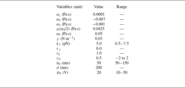

 (a)
 Ω
 K
 (b)
 ψ0
 T=21

 (ai)
 (bi)
 (ci)
 ψ0
 ν=0.25
 h0
 ii
 iii
 (kf=εd=αi(i≠4)=0)
 T=21

 (ai−aiii)
 ν=0.45
 (ai)
 T=21
 (aii)
 T=21
 (aiii)
 T=21
 (bi)
 Tr
 Arp,Ars
 Ar
 Tr
 ν
 (bii)
 (biii)

 ψ0=20
 (a)
 h0
 d
 Ars
 (b−d),
 (e)

 (ai)
 (aii)
 Ar
 (aiii)
 εd
 (bi)
 εd
 <
 (bii)
 εd
 >
 Ar
 εd
 (biii)

 ψ0
 (ai)
 (aii)
 Ar
 Er
 ψ0
 kf=
 (aiii)
 (bi)
 kf
 =0.5
 (bii)
 kf
 =
 Ar
 Er
 kf
 ψ0=20
 (biii)

 Ars
 (a)
 θbottom−top
 ν
 Er=354
 (b) θbottom−top−Er
 ν=0.25
 (c) θbottom−top−Er−ν

 ν
 (a)
 ν=0.62
 (bi)
 ψ0
 (bii)
 ψ0
 T=21

 (a)
 ν=0.62
 ψ0=20
 Δθ=90
 ∘
 θ
 (b)



