1 Introduction
In fluid mechanics, energy budgets provide useful insights into the mechanisms at play in the energy cascade, the transfer from the large scale of energy injection to the small scales where dissipation is taking place. In geophysical and astrophysical systems, it is of paramount importance to understanding the role played by internal gravity waves, generated through different mechanisms at large scale, in the induced mixing of the fluid occurring at small scales (Munk Reference Munk1966; Munk & Wunsch Reference Munk and Wunsch1998; Ivey, Winters & Koseff Reference Ivey, Winters and Koseff2008; André, Mathis & Barker Reference André, Mathis and Barker2019; Sutherland et al. Reference Sutherland, Achatz, Caulfield and Klymak2019).
Recently, there has been a lot of interest in the determination of the injected energy flux into the internal wave field which requires the simultaneous measurement of both velocity and pressure fields. Direct calculations can be rather straightforwardly performed in numerical simulations, since both fields are computed (Lamb Reference Lamb2004; Mathur & Peacock Reference Mathur and Peacock2009; Rapaka, Gayen & Sarkar Reference Rapaka, Gayen and Sarkar2013). This is usually much more complicated in laboratory experiments and even more so in field measurements where we can have at best the information on a one-dimensional line (van Haren & Gostiaux Reference van Haren and Gostiaux2012). Different methods have, however, been proposed depending on the experimental techniques used to visualize the internal waves. Lee et al. (Reference Lee, Paoletti, Swinney and Morrison2014) require only the velocity field measured using the particle image velocimetry (PIV) technique. Density perturbations obtained with the synthetic schlieren technique can lead to the estimation of the energy flux for linear (Clark & Sutherland Reference Clark and Sutherland2010; Allshouse et al. Reference Allshouse, Lee, Morrison and Swinney2016) or nonlinear stratifications (Lee et al. Reference Lee, Allshouse, Swinney and Morrison2018). Finally, Nash, Alford & Kunze (Reference Nash, Alford and Kunze2005) present a method to compute the energy flux from ocean observations.
The counterpart of the energy sources is the energy sinks. In the ocean, it has been observed that the loss of energy can occur very far from the energy sources. Even if some energy is lost during propagation, some dissipation occurs near topographies, indicating that what is happening near boundaries clearly matters in the global energy budget (Nikurashin & Ferrari Reference Nikurashin and Ferrari2010). Indeed, small streamwise undulations of a bottom topography may have an effect on the structure of the viscous boundary layer (Passaggia, Meunier & Le Dizès Reference Passaggia, Meunier and Le Dizès2014) and can induce a decay of internal tides in the ocean (Buhler & Holmes-Cerfon Reference Buhler and Holmes-Cerfon2011). In laboratory experiments, the propagation of an internal wave beam is affected by viscous damping, as initially studied by Thomas & Stevenson (Reference Thomas and Stevenson1973), or through instabilities of internal wave beams (Dauxois et al. Reference Dauxois, Joubaud, Odier and Venaille2018). It has been also recently shown that viscous boundary layers can induce strong mean flow due to streaming (Horne et al. Reference Horne, Beckebanze, Micard, Odier, Maas and Joubaud2019; Renaud & Venaille Reference Renaud and Venaille2019).
In a recent paper, Beckebanze et al. (Reference Beckebanze, Brouzet, Sibgatullin and Maas2018) investigate the role of the boundary layers in the resulting spectrum of an internal wave field attractor. The latter for stratified fluids or inertial wave attractors for rotating fluids are a very interesting scenario for energy transfer since energy is linearly transferred through smaller scales due to the focusing on a sloping topography (Dauxois & Young Reference Dauxois and Young1999). Depending on the geometry of the domain, multiple reflections can lead to a concentration of wave energy on a closed loop, the so-called internal wave attractor (Maas & Lam Reference Maas and Lam1995; Maas et al. Reference Maas, Benielli, Sommeria and Lam1997). In the presence of dissipation, the width of the attractor beam is set by the competition between geometric focusing and viscous broadening (Rieutord, Georgeot & Valdettaro Reference Rieutord, Georgeot and Valdettaro2001; Ogilvie Reference Ogilvie2005; Grisouard, Staquet & Pairaud Reference Grisouard, Staquet and Pairaud2008; Hazewinkel et al. Reference Hazewinkel, van Breevoort, Dalziel and Maas2008). Beckebanze et al. (Reference Beckebanze, Brouzet, Sibgatullin and Maas2018) model the different dissipation processes and, in particular, take into account the part due to viscous boundary layers. They finally describe with a very good agreement the spectrum of linear internal wave attractors obtained in previous laboratory experiments (Hazewinkel et al. Reference Hazewinkel, van Breevoort, Dalziel and Maas2008; Brouzet et al. Reference Brouzet, Sibgatullin, Scolan, Ermanyuk and Dauxois2016b ). Furthermore, a high concentration of energy makes attractors prone to different instabilities (Maas Reference Maas2005). Several experiments have recently shown the scenario of instability that can occur in internal wave attractors (Scolan, Ermanyuk & Dauxois Reference Scolan, Ermanyuk and Dauxois2013; Brouzet et al. Reference Brouzet, Ermanyuk, Joubaud, Sibgatullin and Dauxois2016a , Reference Brouzet, Ermanyuk, Joubaud, Pillet and Dauxois2017) which involves in particular the triadic resonance instability (Dauxois et al. Reference Dauxois, Joubaud, Odier and Venaille2018). The effect of these nonlinearities on the dissipation rate for the attractor has been studied numerically by Jouve & Ogilvie (Reference Jouve and Ogilvie2014).
In the present paper, we consider experimentally the complete energy budget for an internal wave attractor in a trapezoidal geometry. Measuring the velocity field only in the bulk (i.e. outside the boundary layers), we carefully show how to quantify the injected power and the energy sink. Both the internal shear layer and the boundary layers are taken into account. We analyse the complete energy budget in two linear scenarios but also in a nonlinear scenario involving a cascade of triadic resonance instabilities.
The paper is organized as follows. Once the experimental set-up used in the laboratory has been described in § 2, we introduce in § 3 the corresponding energy budget model. The injection energy flux and the different terms involved in the dissipation rate are then presented. In § 4, we first carefully measure and analyse the energy balance in a linear case. In a second stage, when considering nonlinear regimes, we demonstrate that secondary waves emerging in the energy cascade account for a non-negligible part of the total dissipation. The importance of the dissipation in the boundary layers is then discussed using a linear internal wave attractor in a different experimental set-up. We finally conclude in § 5 and draw some perspectives.
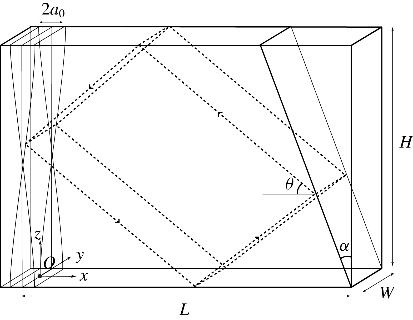
Schematic view in perspective of the experimental set-up. A sloping wall, inclined at an angle
 $\unicode[STIX]{x1D6FC}$
with respect to the vertical, is put inside an immobile tank delimiting a trapezoidal fluid domain of length
 $L=1720~\text{mm}$
(measured along the bottom), depth
 $H=920~\text{mm}$
and thickness
 $W=170~\text{mm}$
. A flexible membrane is oscillating around an axis located at mid-height, producing a horizontal velocity field
 $a_{0}\sin (\unicode[STIX]{x1D714}_{0}t)\cos (\unicode[STIX]{x03C0}z/H)$
. Black dotted lines show an internal wave billiard geometric prediction of an attractor of frequency
 $\unicode[STIX]{x1D714}_{0}$
. The angle
 $\unicode[STIX]{x1D703}$
of the first branch (top right) is given by the dispersion relation
 $\unicode[STIX]{x1D714}_{0}=N\sin \unicode[STIX]{x1D703}$
. The origin
 $O$
is taken at the bottom left part of the fluid domain, at mid-width.

2 Experimental set-up
As shown in figure 1, a rectangular tank of size
 $L\times W\times H=2000\times 170\times 1000~\text{mm}^{3}$
is filled with a fluid linearly stratified with salt and for which the density varies from
 $1.06~\text{kg}~\text{l}^{-1}$
at the bottom to
 $1.00~\text{kg}~\text{l}^{-1}$
at the surface. The origin
 $O$
and the coordinates
 $x$
,
 $y$
(horizontal) and
 $z$
(vertical) are defined in figure 1. The buoyancy frequency, defined as
 $N=\sqrt{-(g/\unicode[STIX]{x1D70C}_{r})\,\text{d}\unicode[STIX]{x1D70C}_{0}(z)/\text{d}z}$
, in which
 $\unicode[STIX]{x1D70C}_{0}(z)$
is the density stratification at rest and
 $\unicode[STIX]{x1D70C}_{r}$
is the averaged density of the stratified region, is chosen at
 $0.68\pm 0.02~\text{rad}~\text{s}^{-1}$
. A sloping wall, tilted by an angle
 $\unicode[STIX]{x1D6FC}$
with respect to the vertical, delimits a trapezoidal fluid domain of length
 $L=1720~\text{mm}$
(measured along the bottom) and depth
 $H=920~\text{mm}$
. The system is forced by an internal wave generator (left wall) of the same height
 $H$
made of a flexible membrane pivoting around an axis at mid-height. The top and bottom ends remain vertical and are oscillating at the frequency
 $\unicode[STIX]{x1D714}_{0}$
with an amplitude
 $a_{0}$
. These two parameters can be tuned appropriately by a simple electro-mechanical device. The frequency is chosen to be constant throughout all experiments described here while different amplitudes are used but kept constant during each of them. The position of the flexible membrane can thus be given with a very good agreement by
 $a_{0}\sin (\unicode[STIX]{x1D714}_{0}t)\cos (\unicode[STIX]{x03C0}z/H)$
, where
 $z$
is the vertical coordinate taken from the bottom of the tank. Due to the shape of the generator, the vertical component of the induced wavevector is given by
 $m=2\unicode[STIX]{x03C0}/\unicode[STIX]{x1D706}_{z}=2\unicode[STIX]{x03C0}/(2H)$
while the horizontal one,
 $\ell =2\unicode[STIX]{x03C0}\unicode[STIX]{x1D714}_{0}/(N\unicode[STIX]{x1D706}_{z}\sqrt{1-(\unicode[STIX]{x1D714}_{0}/N)^{2}})$
, is obtained using the dispersion relation
 $\unicode[STIX]{x1D714}_{0}=N\ell /\sqrt{\ell ^{2}+m^{2}}=N\sin \unicode[STIX]{x1D703}$
, with
 $\unicode[STIX]{x1D703}$
the angle between the wavevector and the vertical. Note that this angle is also equal to the angle between the rays and the horizontal as displayed in figure 1, where rays are energy propagation paths. The typical wavelength of the injected wave field
 $2H\sqrt{1-(\unicode[STIX]{x1D714}_{0}/N)^{2}}$
is of the order of
 $1500~\text{mm}$
.
The experimental set-up has been designed such that the wave field is quasi-bidimensional. This means that the transverse velocity field
 $v$
can be considered null and that the horizontal and vertical components of the velocity field, denoted
 $u$
and
 $w$
, do not depend on the transverse direction
 $y$
, except in the boundary layers. This property has been experimentally and numerically verified for the linear and weakly nonlinear regimes in Brouzet et al. (Reference Brouzet, Sibgatullin, Scolan, Ermanyuk and Dauxois2016b
).
The velocity field (
 $u$
,
 $w$
) measured in the vertical mid-plane (
 $y=0$
) is then monitored as a function of spatial coordinates and time, using the standard PIV technique. The flow is indeed seeded with
 $10$
 $\unicode[STIX]{x03BC}\text{m}$
silver-coated hollow glass spheres of density
 $1.4~\text{kg}~\text{m}^{-3}$
, and illuminated by a 532 nm 2 W continuous laser shaped into a vertical sheet. The cross-correlation algorithm (Fincham & Delerce Reference Fincham and Delerce2000) is performed by analysing windows of typical size
 $31\times 31$
pixels with
 $20$
% overlap. The final mesh size is approximately 1 cm.
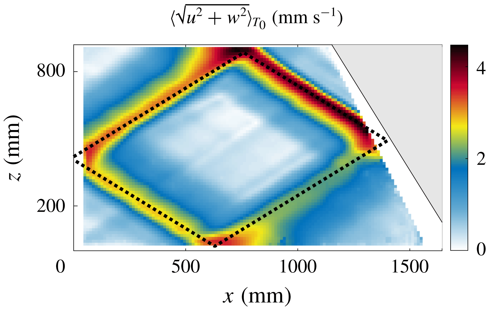
Figure 2 presents a typical experimental measurement of the amplitude of the velocity field measured in the steady state and within the linear regime. We clearly see that the velocity field is focused around the infinitely thin inviscid theoretical attractor, depicted by the dashed line, with counterclockwise energy propagation. Note that the PIV images show a different pattern from the ones obtained using synthetic schlieren (Scolan et al. Reference Scolan, Ermanyuk and Dauxois2013; Brouzet et al. Reference Brouzet, Sibgatullin, Scolan, Ermanyuk and Dauxois2016b ). Indeed, this last technique, being sensible to the gradient of the density, emphasizes the small scales. As we are interested in the energy budget, the PIV technique is more appropriate as we will consider the viscous dissipation, which depends only on the velocity field.
The finite width
 $\unicode[STIX]{x1D706}$
of the attractor (approximately 100 mm) is the result of the equilibrium between focusing after reflection on the slope and the viscous spreading. The amplitude, which is at least five times larger than the wavemaker velocity
 $a_{0}\unicode[STIX]{x1D714}_{0}$
, attains its maximum just after the focalization on the inclined slope: this is the start of the first branch of the attractor. The amplitude gradually decreases along the attractor to end in the fourth branch, of small amplitude and with a rather large width. After reflection on the slope, the fourth branch is focussed again and we recover the first branch, thin and with a large amplitude. The dissipation along the attractor is precisely balanced by the focussing and we get a stable limit cycle, the internal wave attractor.
Spatial evolution within the tank of the amplitude of the velocity field
 $\langle \sqrt{u^{2}+w^{2}}\rangle _{T_{0}}$
, averaged over 10 forcing periods
 $T_{0}=2\unicode[STIX]{x03C0}/\unicode[STIX]{x1D714}_{0}$
around
 $t=50T_{0}$
. The theoretically expected attractor for this geometry is depicted with the dashed line. The parameters of the experiment are
 $a_{0}=2~\text{mm}$
,
 $\unicode[STIX]{x1D714}_{0}/N=0.52$
,
 $N=0.68\pm 0.02~\text{rad}~\text{s}^{-1}$
and
 $\unicode[STIX]{x1D6FC}=29.5^{\circ }$
. Note that the shadow of the slope modifies the illumination of the laser sheet and therefore hinders the measurement of the velocity field in the region very close to the slope: this is why a mask (in white in the figure) with an angle different from the slope angle has been chosen to avoid ambiguous measurements in this region.

Now that the experimental set-up has been presented in detail, we will carefully discuss the different contributions involved in the energy budget of internal wave attractor experiments.
3 Model
3.1 Energy budget
Let us consider an incompressible, non-rotating, stratified fluid in Cartesian coordinates
 $(\boldsymbol{e}_{x},\boldsymbol{e}_{y},\boldsymbol{e}_{z})$
, where
 $\boldsymbol{e}_{z}$
is the direction opposite to gravity. In the framework of the Boussinesq approximation, the equations of motion can be written as
 $$\begin{eqnarray}\displaystyle & \displaystyle \unicode[STIX]{x2202}_{t}\boldsymbol{u}+\boldsymbol{u}\boldsymbol{\cdot }\unicode[STIX]{x1D735}\boldsymbol{u}=-\frac{1}{\unicode[STIX]{x1D70C}_{r}}\unicode[STIX]{x1D735}P+b\boldsymbol{e}_{\boldsymbol{z}}+\unicode[STIX]{x1D708}\unicode[STIX]{x1D6FB}^{2}\boldsymbol{u}, & \displaystyle\end{eqnarray}$$
 $$\begin{eqnarray}\displaystyle & \displaystyle \unicode[STIX]{x2202}_{t}b+\boldsymbol{u}\boldsymbol{\cdot }\unicode[STIX]{x1D735}b=-wN^{2}, & \displaystyle\end{eqnarray}$$
 $$\begin{eqnarray}\displaystyle & \displaystyle \unicode[STIX]{x1D735}\boldsymbol{\cdot }\boldsymbol{u}=0, & \displaystyle\end{eqnarray}$$
in which
 $\boldsymbol{u}=(u,v,w)$
is the fluid velocity field,
 $\unicode[STIX]{x1D70C}_{r}$
the average density over the stratified region,
 $P$
the pressure variation with respect to the hydrostatic equilibrium pressure,
 $b=g(\unicode[STIX]{x1D70C}_{0}-\unicode[STIX]{x1D70C})/\unicode[STIX]{x1D70C}_{r}$
the perturbed buoyancy field,
 $N$
the buoyancy frequency and
 $\unicode[STIX]{x1D708}$
the kinematic viscosity.
In (3.2), we have neglected the molecular diffusivity, which would imply a term
 $D\unicode[STIX]{x1D6FB}^{2}b$
with
 $D$
the diffusion coefficient of the stratifying element. As we discussed, laboratory experiments use salt as the stratification agent, so
 $D\simeq 10^{-9}~\text{m}^{2}~\text{s}^{-1}$
which corresponds to a Schmidt number of
 $\unicode[STIX]{x1D708}/D\sim 10^{3}$
. Therefore, this term can be neglected with respect to the viscous term appearing in (3.1).
Let us recall how it is possible to establish the energy budget of this system as a balance between the injected power and the dissipation rate (see for example Kundu (Reference Kundu1990)). Multiplying (3.1) with
 $\boldsymbol{u}$
and integrating over
 ${\mathcal{V}}$
, the whole volume of the tank (bounded by the surface
 ${\mathcal{S}}$
) and using (3.2), we get
 $$\begin{eqnarray}\displaystyle \unicode[STIX]{x2202}_{t}\int _{{\mathcal{V}}}\,\text{d}V\left(\frac{\boldsymbol{u}^{2}}{2}+\frac{1}{N^{2}}\frac{b^{2}}{2}\right) & = & \displaystyle -\frac{1}{\unicode[STIX]{x1D70C}_{r}}\int _{{\mathcal{V}}}\,\text{d}V\boldsymbol{u}\boldsymbol{\cdot }\unicode[STIX]{x1D735}P-\int _{{\mathcal{V}}}\,\text{d}V\boldsymbol{u}\boldsymbol{\cdot }\unicode[STIX]{x1D735}\left(\frac{\boldsymbol{u}^{2}}{2}+\frac{1}{N^{2}}\frac{b^{2}}{2}\right)\nonumber\\ \displaystyle & & \displaystyle +\,\unicode[STIX]{x1D708}\int _{{\mathcal{V}}}\,\text{d}V\boldsymbol{u}\boldsymbol{\cdot }\unicode[STIX]{x1D6FB}^{2}\boldsymbol{u},\end{eqnarray}$$
where
 $\int _{{\mathcal{V}}}$
and
 $\unicode[STIX]{x2202}_{t}$
have been commuted. Indeed, the length of the tank varies only by
 $\unicode[STIX]{x0394}L/L\sim 0.1\,\%$
, with a typical time of variation
 $t_{L}=T_{0}$
. We will see in figure 7 in § 4 that the integrand increases from zero to its final value on a typical time
 $t_{e}\sim 10T_{0}$
, such that
 $\unicode[STIX]{x0394}L/(Lt_{L})\ll 1/t_{e}$
. The variations of the frontiers of
 ${\mathcal{V}}$
are thus sufficiently small and slow and can be neglected.
The left-hand side is the variation of the total energy
 $E_{tot}$
that corresponds to the sum of the kinetic and potential energies within the fluid. Note that the latter is defined with respect to the reference stratification which is supposed fixed, no mixing being taken into account.
Let us show that the right-hand side corresponds to the sum of the energy injection rate and the viscous dissipation rate. We will first focus on the monochromatic case, before considering the polychromatic one in § 4.2. First of all, we turn the volume integral into a surface integral, keeping in mind that, in an incompressible flow, the velocity field satisfies the continuity equation
 $\unicode[STIX]{x1D735}\boldsymbol{\cdot }\boldsymbol{u}=0.$
Denoting
 $\text{d}\boldsymbol{S}$
the element of surface which normal is oriented out of the fluid, the first term can therefore be rewritten as
 $$\begin{eqnarray}\displaystyle -\int _{{\mathcal{V}}}\,\text{d}V\boldsymbol{u}\boldsymbol{\cdot }\unicode[STIX]{x1D735}P & = & \displaystyle \int _{{\mathcal{V}}}\,\text{d}VP\unicode[STIX]{x1D735}\boldsymbol{\cdot }\boldsymbol{u}-\oint _{{\mathcal{S}}}P\boldsymbol{u}\boldsymbol{\cdot }\text{d}\boldsymbol{S}\nonumber\\ \displaystyle & = & \displaystyle -\int _{{\mathcal{S}}_{g}}P\boldsymbol{u}\boldsymbol{\cdot }\text{d}\boldsymbol{S},\end{eqnarray}$$
using the property that the component of the velocity normal to the surface
 ${\mathcal{S}}$
vanishes everywhere except on
 ${\mathcal{S}}_{g}$
, the surface of the wave generator where the flexible membrane injects energy into the tank.
In the same way, the second term of the right-hand side of (3.4) is equal to the energy flux at the boundaries of the domain. Using similar arguments, only the surface of the generator has to be considered. Both quantities
 $\boldsymbol{u}^{2}\boldsymbol{u}$
and
 $b^{2}\boldsymbol{u}$
thus vanish when averaged over the forcing period
 $T_{0}=2\unicode[STIX]{x03C0}/\unicode[STIX]{x1D714}_{0}$
, as they are an odd power of a trigonometric function. The second term of the right-hand side of (3.4) is thus equal to zero.
Turning again the volume integral into a surface integral, the last term on the right-hand side of (3.4) yields
 $$\begin{eqnarray}\unicode[STIX]{x1D708}\int _{{\mathcal{V}}}\,\text{d}V\boldsymbol{u}\boldsymbol{\cdot }\unicode[STIX]{x1D6FB}^{2}\boldsymbol{u}=-\unicode[STIX]{x1D708}\int _{{\mathcal{V}}}\,\text{d}V|\unicode[STIX]{x1D735}\boldsymbol{u}|^{2}+\unicode[STIX]{x1D708}\oint _{{\mathcal{S}}}u_{i}\unicode[STIX]{x2202}_{j}u_{i}\,\text{d}S_{j}.\end{eqnarray}$$
The last term vanishes when considering fixed solid boundaries (right slope and bottom) using the no-slip and no-penetration conditions. It vanishes also at the surface, due to the free-slip condition and because there is no normal variation of the normal velocity, even in the presence of small surface waves. For the remaining boundary – the generator – the velocity field corresponds essentially to a mode-1 induced by the generator itself. Both quantities
 $u\unicode[STIX]{x2202}_{x}u$
and
 $w\unicode[STIX]{x2202}_{x}w$
have thus a vanishing average on the forcing period
 $T_{0}=2\unicode[STIX]{x03C0}/\unicode[STIX]{x1D714}_{0}$
while
 $v=0$
.
Equation (3.3) is thus rewritten as the energy budget within the tank
 $$\begin{eqnarray}\unicode[STIX]{x2202}_{t}e_{tot}=p_{inj}-p_{diss},\end{eqnarray}$$
which relates, per unit mass, the time variation of the total energy
 $e_{tot}\equiv E_{tot}/{\mathcal{V}}$
with the injected power
 $$\begin{eqnarray}p_{inj}\equiv -\frac{1}{\unicode[STIX]{x1D70C}_{r}{\mathcal{V}}}\int _{{\mathcal{S}}_{g}}P\boldsymbol{u}\boldsymbol{\cdot }\text{d}\boldsymbol{S}\end{eqnarray}$$
and the dissipation rate
 $$\begin{eqnarray}p_{diss}\equiv \frac{\unicode[STIX]{x1D708}}{{\mathcal{V}}}\int _{{\mathcal{V}}}\,\text{d}V|\unicode[STIX]{x1D735}\boldsymbol{u}|^{2}.\end{eqnarray}$$
For convenience, it is useful to introduce the local density of dissipation rate
 $\unicode[STIX]{x1D716}\equiv \unicode[STIX]{x1D708}|\unicode[STIX]{x1D735}\boldsymbol{u}|^{2}$
. A temporal average over an integer number of forcing periods
 $T_{0}$
will be considered. The method to determine the time-averaged values of the total energy, the injected power and the dissipation rate requires only the velocity field data and will be presented in the following section.
3.2 Estimation of the different terms from experimental measurements
3.2.1 Total energy
Unlike rotating inertial waves, where no potential energy can be defined, equipartition of energy between kinetic and potential subparts can be defined for internal waves. The time variation of the total energy can thus be safely obtained from PIV that gives accurate measurements of the velocity components:
 $\langle e_{tot}\rangle _{T_{0}}=\int _{{\mathcal{V}}}\,\text{d}V\langle \boldsymbol{u}^{2}\rangle _{T_{0}}/{\mathcal{V}}$
.
The velocity field has been shown to be bidimensional (i.e. only two components invariant in the
 $y$
-direction) except in the boundary layers, of typical width
 $d=\sqrt{\unicode[STIX]{x1D708}/\unicode[STIX]{x1D714}_{0}}\sim 1~\text{mm}$
(Brouzet et al.
Reference Brouzet, Sibgatullin, Scolan, Ermanyuk and Dauxois2016b
). So their total volume,
 $2d{\mathcal{A}}+d{\mathcal{L}}W$
(where
 ${\mathcal{L}}$
is the perimeter of the vertical trapezoidal section of the domain,
 ${\mathcal{A}}$
its area and
 $W$
the width of the experimental tank) represents only
 $1$
% of the total volume of the tank. The measured value of the total energy will thus be computed as
 $\langle e_{tot}\rangle _{T_{0}}=\int _{{\mathcal{A}}}\,\text{d}x\,\text{d}z\langle \boldsymbol{u}^{2}\rangle _{T_{0}}/{\mathcal{A}}$
, where
 $\boldsymbol{u}$
is measured in the mid vertical plane only.
Because of some experimental issues near boundaries, the measured area is a bit smaller than the total area of the trapezoidal domain. However since this difference is small we assume that the sampled area is representative enough so that our measure of the average energy density is correct.
3.2.2 Injected power
As the generator is everywhere almost vertical, we can safely approximate (3.8) by
 $$\begin{eqnarray}p_{inj}\simeq \frac{1}{\unicode[STIX]{x1D70C}_{r}{\mathcal{A}}}\int _{z}Pu\,\text{d}z.\end{eqnarray}$$
The determination of the injected power requires therefore the simultaneous measurement of the horizontal velocity field and the pressure near the wavemaker on the left boundary of the tank (
 $x=0$
). This kind of generator forces a purely propagating mode-1 with an amplitude
 $u_{0}$
slightly lower than
 $a_{0}\unicode[STIX]{x1D714}_{0}$
depending on the efficiency of the wavemaker (see Mercier et al.
Reference Mercier, Martinand, Mathur, Gostiaux, Peacock and Dauxois2010),
 $$\begin{eqnarray}\displaystyle u^{M1}(x,z,t)=u_{0}\cos (mz)\cos (\unicode[STIX]{x1D714}_{0}t-\ell x). & & \displaystyle\end{eqnarray}$$
Using the incompressibility equation and assuming that the flow is two-dimensional, we can straightforwardly get the vertical component,
 $$\begin{eqnarray}\displaystyle w^{M1}(x,z,t)=-u_{0}\frac{\ell }{m}\sin (mz)\sin (\unicode[STIX]{x1D714}_{0}t-\ell x), & & \displaystyle\end{eqnarray}$$
induced in the fluid by the generator. The associated pressure field can be deduced by projection of the linear inviscid version of (3.1) on the
 $x$
-axis, followed by a straightforward integration
 $$\begin{eqnarray}P^{M1}(x,z,t)=\unicode[STIX]{x1D70C}_{r}u_{0}\frac{\unicode[STIX]{x1D714}_{0}}{\ell }\cos (mz)\cos (\unicode[STIX]{x1D714}_{0}t-\ell x),\end{eqnarray}$$
in which the constant of integration is set to zero since
 $P$
accounts only for the pressure variation with respect to the hydrostatic equilibrium pressure. The time-averaged theoretically injected power can then be computed as
 $$\begin{eqnarray}\langle p_{inj}^{M1}\rangle _{T_{0}}=u_{0}^{2}N\frac{H^{2}}{4\unicode[STIX]{x03C0}}\sqrt{1-\left(\frac{\unicode[STIX]{x1D714}_{0}}{N}\right)^{2}}\frac{1}{{\mathcal{A}}}.\end{eqnarray}$$
This theoretical development is valid for a pure propagating mode-1. However, such approximation may be questioned in the presence of the slope, since the size of the closed domain has been chosen to get strong reflected beams, which are required for the formation of the attractor. Some feedback on the forced wave field from its reflection on the slope is then expected.
To go beyond, it is possible to use the PIV measurements to compute both the pressure and horizontal velocity appearing in (3.10). Indeed, if the PIV technique gives directly the horizontal velocity field, the pressure field can be obtained from
 $u$
and
 $w$
as follows. Since the width of the attractor
 $\unicode[STIX]{x1D706}$
, which is the typical length of variation of the velocity field in the transverse direction of the branch, is much larger than
 $d$
, we use the linear and inviscid approximation of (3.1) and (3.2) to get the experimental pressure gradient, which is then integrated using the Matlab© code intgrad2, available at www.mathworks.com/matlabcentral/fileexchange/. The unknown constant of integration necessary for this last step is not important since mass conservation implies
 $\int _{{\mathcal{S}}_{g}}u\,\text{d}y\,\text{d}z=0$
, leading to a vanishing contribution to the injected power. Thus we arbitrarily choose
 $\langle P\rangle _{{\mathcal{A}}}=0$
.
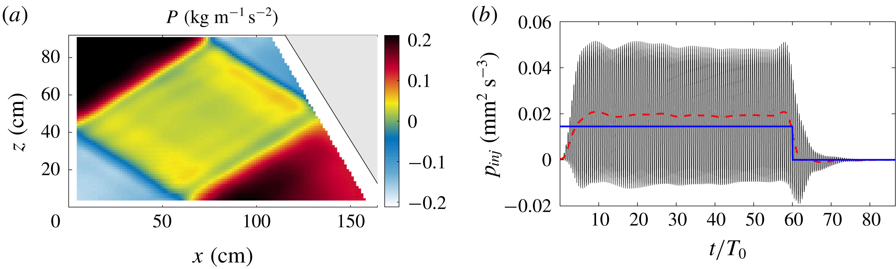
An example of the computed pressure field is presented in figure 3(a). The pressure field is different from the pure mode-1 pattern (3.13): this will have some consequences on the estimation of the injected power. Because of the integration, the pressure field emphasizes the large scale motion contrary to the density gradient or velocity fields that show the attractor (see for example figure 2).
(a) Pressure field
 $P$
, computed via an integration of the experimental velocity fields
 $u$
and
 $w$
. The unimportant constant of integration is arbitrarily chosen to have a zero average pressure field. The pattern is computed approximately
 $50T_{0}$
after the generator was started. (b) Evolution in time of the injected power computed at
 $x_{0}=5~\text{cm}$
. The oscillating black curve corresponds to the instantaneous measurement, while the red dashed curve is the associated local mean. The generator is switched on at
 $t=0$
while it is turned off at
 $t=60T_{0}$
. The thick blue line corresponds to the theoretical injected power (3.14) expected for a pure mode-1, i.e. neglecting the reflection on the slope. Experimental parameters are those given in the caption of figure 2.

Figure 3(b) shows the time evolution of the injected power
 $p_{inj}$
(solid black line) for a typical experiment in the linear regime. For visualization purposes, this flux of energy is measured at
 $x_{0}\simeq 5~\text{cm}$
, as will be discussed in § 4.1;
 $p_{inj}$
is oscillating with a mean value (dashed line) that first increases until reaching its stationary value. As soon as the generator is turned off, it decreases towards zero. We note that the measured value is above
 $\langle p_{inj}^{M1}\rangle _{T_{0}}$
(thick blue line), i.e. the theoretical injected power (3.14) expected for a pure mode-1 neglecting the finite size of the domain due to the reflection on the slope.
3.2.3 Disentangling the different contributions for the dissipative terms
As already mentioned, the two-dimensional PIV measurements give access to the velocity field in the middle plane
 $y=0$
and can be extended to the volume except in the boundary layers. In the remainder of the paper, this is named the bulk part. Since the thickness of the boundary layers is very small, the velocity gradient may be strong in these regions and the associated dissipative term cannot be neglected. It is therefore convenient to distinguish several different contributions as follows:
 $$\begin{eqnarray}\displaystyle p_{diss} & = & \displaystyle \frac{1}{{\mathcal{V}}}\int _{{\mathcal{V}}}\,\text{d}V\unicode[STIX]{x1D708}|\unicode[STIX]{x1D735}\boldsymbol{u}|^{2}\nonumber\\ \displaystyle & = & \displaystyle \underbrace{\frac{1}{{\mathcal{V}}}\int _{{\mathcal{V}}_{bulk}}\,\text{d}V\underbrace{\unicode[STIX]{x1D708}|\unicode[STIX]{x1D735}\boldsymbol{u}|^{2}}_{\unicode[STIX]{x1D716}_{bulk}}}_{p_{bulk}}+\underbrace{\frac{1}{{\mathcal{V}}}\int _{{\mathcal{V}}_{BL,\bot }}\,\text{d}V\underbrace{\unicode[STIX]{x1D708}|\unicode[STIX]{x1D735}\boldsymbol{u}|^{2}}_{\unicode[STIX]{x1D716}_{\bot }}}_{p_{\bot }}+\underbrace{\frac{1}{{\mathcal{V}}}\int _{{\mathcal{V}}_{BL,\Vert }}\,\text{d}V\underbrace{\unicode[STIX]{x1D708}|\unicode[STIX]{x1D735}\boldsymbol{u}|^{2}}_{\unicode[STIX]{x1D716}_{\Vert }}}_{p_{\Vert }}.\qquad\end{eqnarray}$$
This definition disentangles the bulk dissipation (denoted with the index bulk and that we can expect to measure accurately), from the contributions of the boundary layers close to the walls. Among the last ones, we distinguish the dissipation in the boundary layers along the longitudinal walls (parallel to the measurement plane and therefore perpendicular to
 $y$
, denoted with the index
 $\Vert$
), from the dissipation in the boundary layers perpendicular to the attractor plane (denoted with the index
 $\bot$
). Let us discuss these three different terms successively.
In the bulk, the transverse velocity
 $v$
is equal to zero and the velocity components
 $u$
and
 $w$
do not depend on
 $y$
. The contribution of the bulk can thus be computed rather straightforwardly from the measurements of the velocity field shown in figure 2 using the formula
 $$\begin{eqnarray}\unicode[STIX]{x1D716}_{bulk}=\unicode[STIX]{x1D708}|\unicode[STIX]{x1D735}\boldsymbol{u}|^{2}=\unicode[STIX]{x1D708}(\unicode[STIX]{x2202}_{x}u)^{2}+\unicode[STIX]{x1D708}(\unicode[STIX]{x2202}_{z}u)^{2}+\unicode[STIX]{x1D708}(\unicode[STIX]{x2202}_{x}w)^{2}+\unicode[STIX]{x1D708}(\unicode[STIX]{x2202}_{z}w)^{2}.\end{eqnarray}$$
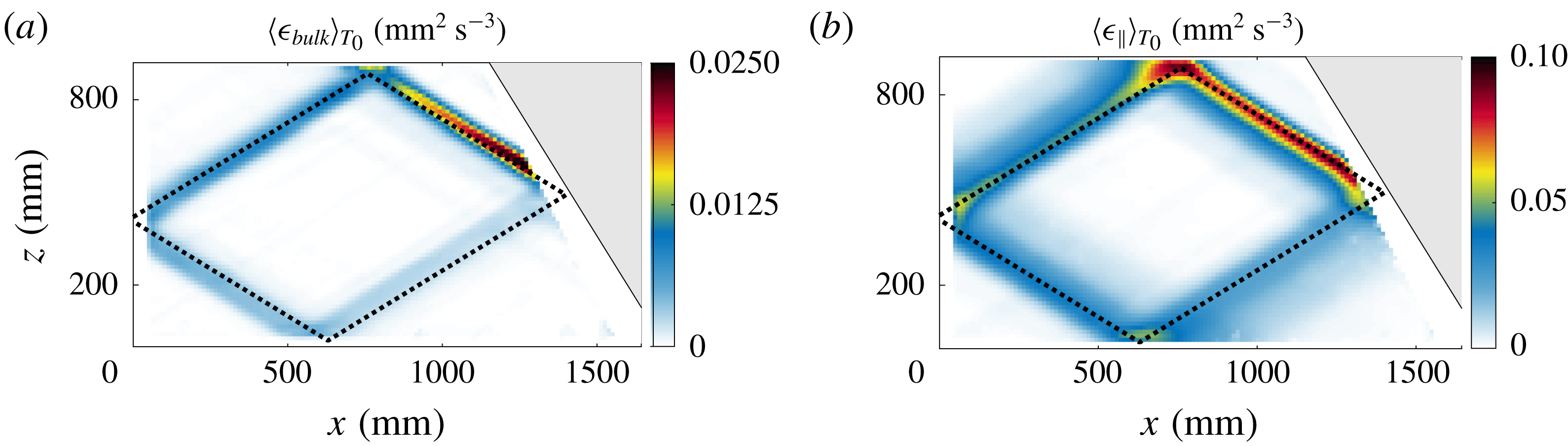
Figure 4(a) presents the spatial dependence of this quantity in the mid-plane averaged over 10
 $T_{0}$
. As expected, its amplitude is particularly important along the first branch of the attractor, that is located just after the reflection on the slope where the focusing takes place, and then decreases along the attractor. The mean of this quantity on the whole domain leads to
 $p_{bulk}$
, the energy dissipation rate due to the bulk.
It is much more difficult to directly estimate the dissipation in the boundary layers. Indeed, since their thicknesses are very small compared to the size of the tank (approximately
 $1$
%), it is very hard to measure the velocity in the boundary layers as accurately as in the bulk. A method to evaluate the velocity using the velocity measured in the mid-plane (
 $y=0$
) will then be presented for the two types of boundary layer, parallel to the lateral walls (§ 3.2.4) and perpendicular to the attractor plane (§ 3.2.5). In both cases, theoretical developments recently reported by Beckebanze et al. (Reference Beckebanze, Brouzet, Sibgatullin and Maas2018) will be used and adapted. For the sake of brevity and clarity, only the main ingredients of their results will be recalled. Notice that linear equations will be used in the two following sections as the Reynolds number is small in viscous boundary layers. Brouzet et al. (Reference Brouzet, Sibgatullin, Scolan, Ermanyuk and Dauxois2016b
) showed that the experimental velocity field in the parallel boundary layers is compatible with the theoretical description.
(a) Dissipation rate field within the bulk of the fluid,
 $\langle \unicode[STIX]{x1D716}_{bulk}(x,z)\rangle _{T_{0}}$
, measured in the mid-plane. (b) Dissipation rate field in the longitudinal boundary layers,
 $\langle \unicode[STIX]{x1D716}_{\Vert }\rangle _{T_{0}}$
, averaged along the transverse direction. (a,b) The field has been averaged over 10 forcing periods
 $T_{0}$
around
 $t=50T_{0}$
and the theoretically expected attractor for this geometry is depicted with the dashed line. Experimental parameters are those given in the caption of figure 2.

3.2.4 The dissipation in the longitudinal boundary layers
 $\unicode[STIX]{x1D716}_{\Vert }$

Close to both longitudinal vertical walls, the largest contribution to the viscous term
 $\unicode[STIX]{x1D708}\unicode[STIX]{x1D6FB}^{2}\boldsymbol{u}$
comes from the gradients in the
 $y$
-direction. Indeed, experimental measurements show that variations in the
 $xz$
-plane are typically on the centimetre length scale, that is significantly larger than the millimetre length scale that appears in the viscous boundary layer. The evolution of the velocity (3.1) and buoyancy fields (3.2) can thus be simplified as
 $$\begin{eqnarray}\displaystyle & \displaystyle \unicode[STIX]{x2202}_{t}u=-\frac{\unicode[STIX]{x2202}_{x}P}{\unicode[STIX]{x1D70C}_{r}}+\unicode[STIX]{x1D708}\unicode[STIX]{x2202}_{yy}u, & \displaystyle\end{eqnarray}$$
 $$\begin{eqnarray}\displaystyle & \displaystyle \unicode[STIX]{x2202}_{t}w=-\frac{\unicode[STIX]{x2202}_{z}P}{\unicode[STIX]{x1D70C}_{r}}+b+\unicode[STIX]{x1D708}\unicode[STIX]{x2202}_{yy}w, & \displaystyle\end{eqnarray}$$
 $$\begin{eqnarray}\displaystyle & \displaystyle \unicode[STIX]{x2202}_{t}b=-wN^{2}. & \displaystyle\end{eqnarray}$$
The transverse velocity
 $v$
does not vanish any more but its contribution to the dissipation rate remains very small (Beckebanze et al.
Reference Beckebanze, Brouzet, Sibgatullin and Maas2018). Let us consider a monochromatic internal wave
 $a=\text{Re}[\text{}\underline{a}\,\text{e}^{-\text{i}\unicode[STIX]{x1D714}_{0}t}]$
at the frequency
 $\unicode[STIX]{x1D714}_{0}$
in which
 $a$
stands for
 $u$
,
 $w$
,
 $b$
or
 $P$
. The case of polychromatic signals will be discussed in § 4.2. Introducing the angle
 $\unicode[STIX]{x1D703}$
defined through the dispersion relation
 $\unicode[STIX]{x1D714}_{0}^{2}=N^{2}\sin ^{2}\unicode[STIX]{x1D703}$
, (3.19) can be rewritten as
 $\text{}\underline{b}=-\text{i}\unicode[STIX]{x1D714}_{0}\text{}\underline{w}/\text{sin}^{2}\unicode[STIX]{x1D703}$
. Equations (3.17) and (3.18) can then be simplified as
 $$\begin{eqnarray}\displaystyle & \displaystyle -\text{i}\unicode[STIX]{x1D714}_{0}\text{}\underline{u}=-\unicode[STIX]{x2202}_{x}\text{}\underline{P}/\unicode[STIX]{x1D70C}_{r}+\unicode[STIX]{x1D708}\unicode[STIX]{x2202}_{yy}\text{}\underline{u}, & \displaystyle\end{eqnarray}$$
 $$\begin{eqnarray}\displaystyle & \displaystyle \text{i}\unicode[STIX]{x1D714}_{0}\cot ^{2}\unicode[STIX]{x1D703}\text{}\underline{w}=-\unicode[STIX]{x2202}_{z}\text{}\underline{P}/\unicode[STIX]{x1D70C}_{r}+\unicode[STIX]{x1D708}\unicode[STIX]{x2202}_{yy}\text{}\underline{w}, & \displaystyle\end{eqnarray}$$
that have to be solved with the no-slip boundary conditions
 $\text{}\underline{u}(y=\pm W/2)=\text{}\underline{w}(y=\pm W/2)=0$
, while
 $\text{}\underline{u}(y=0)$
and
 $\text{}\underline{w}(y=0)$
can be measured at the centre of the tank with the PIV measurements described above. One finally gets
 $$\begin{eqnarray}\displaystyle & \displaystyle \text{}\underline{u}(y)=\left(1-\frac{\cosh [\text{i}^{1/2}y/d]}{\cosh [\text{i}^{1/2}W/(2d)]}\right)\text{}\underline{u}(y=0), & \displaystyle\end{eqnarray}$$
 $$\begin{eqnarray}\displaystyle & \displaystyle \text{}\underline{w}(y)=\left(1-\frac{\cosh [\text{i}^{-1/2}\cot \unicode[STIX]{x1D703}y/d]}{\cosh [\text{i}^{-1/2}\cot \unicode[STIX]{x1D703}W/(2d)]}\right)\text{}\underline{w}(y=0), & \displaystyle\end{eqnarray}$$
in which we use
 $d=\sqrt{\unicode[STIX]{x1D708}/\unicode[STIX]{x1D714}_{0}}$
, the thickness of the boundary layers.
The dissipation within the longitudinal boundary layers is thus obtained by performing successively the following operations: a time Fourier transform of the wave field in the mid-plane
 $\boldsymbol{u}(x,y=0,z,t)$
, a band-pass filtering in the Fourier space around the forcing frequency
 $\unicode[STIX]{x1D714}_{0}$
, multiplication by the theoretically derived expressions (3.22) and (3.23) with respect to the
 $y$
-coordinate to get
 $\unicode[STIX]{x2202}_{y}\text{}\underline{\boldsymbol{u}}(x,y,z)$
. The real part of the inverse Fourier transform is then taken to generate the signal
 $\unicode[STIX]{x2202}_{y}\boldsymbol{u}(x,y,z)$
. The value of
 $\unicode[STIX]{x1D716}_{\Vert }=\unicode[STIX]{x1D708}[(\unicode[STIX]{x2202}_{y}u)^{2}+(\unicode[STIX]{x2202}_{y}w)^{2}]$
at any point of the domain is then computed and the integration over the whole domain leads to the value of the energy dissipation rate
 $p_{\Vert }=\int \unicode[STIX]{x1D716}_{\Vert }\,\text{d}V/{\mathcal{V}}$
due to the parallel boundary layers. The
 $y$
-averaged value
 $\langle \unicode[STIX]{x1D716}_{\Vert }\rangle _{y,T_{0}}=(1/W)\int _{-W/2}^{+W/2}\,\text{d}y\langle \unicode[STIX]{x1D716}_{\Vert }\rangle _{T_{0}}$
is displayed in figure 4(b) for all points of the domain. Here again, the dissipation is larger along the first branch of the attractor and then decreases along the skeleton of the attractor. By comparing figure 4(a,b), we realize that this boundary layer dissipation is much larger than the bulk dissipation. This difference is a factor of
 $10$
when averaged over the entire domain. Indeed the
 $y$
-averaged dissipation of the bulk is of the order of
 $\unicode[STIX]{x1D708}~(U/\unicode[STIX]{x1D706})^{2}$
, while the
 $y$
-averaged longitudinal boundary layer dissipation is of the order
 $\unicode[STIX]{x1D708}~(2d/W)~(U/d)^{2}$
. We can then estimate the ratio of the two types of dissipation
 $\langle \unicode[STIX]{x1D716}_{bulk}\rangle _{y,T_{0}}/\langle \unicode[STIX]{x1D716}_{\Vert }\rangle _{y,T_{0}}\sim Wd/\unicode[STIX]{x1D706}^{2}\sim 10\,\%$
, a value in good agreement with the measured ratio.
3.2.5 The dissipation in the transversal boundary layers
$\unicode[STIX]{x1D716}_{\bot }$

The second dissipation term in the boundary layers,
 $\unicode[STIX]{x1D716}_{\bot }$
, corresponds to the boundary layers perpendicular to the attractor plane, and, more precisely, where a reflection of the internal wave beam occurs. For the present experimental set-up, three walls have to be considered while, due to the free-slip boundary condition, the reflection at the top surface is not a source of dissipation. Note that no linear coupling between internal and surface waves can occur due to the low frequency which leads to a surface wavelength much larger than the size of the set-up. We have therefore
 $p_{\bot }=p_{\bot }^{[1]}+p_{\bot }^{[3]}+p_{\bot }^{[4]}$
where
 $j=1$
stands for the boundary layer along the slope,
 $j=3$
close to the generator and
 $j=4$
near the bottom of the tank. We will develop the method to estimate the dissipation term associated with a reflection on a wall inclined at an arbitrarily angle
 $\unicode[STIX]{x1D719}$
, that will stand for
 $\unicode[STIX]{x1D6FC}$
,
 $\unicode[STIX]{x03C0}$
or
 $-\unicode[STIX]{x03C0}/2$
respectively for
 $j=1,3,4$
.
Considering the reflection on a boundary in the inviscid case, the velocity field corresponds to the sum of the incident beam
 $\boldsymbol{u}^{[I]}$
and the inviscid reflected beam
 $\boldsymbol{u}^{[R]}$
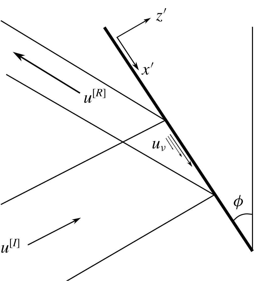
. It has to fulfil the no-penetration condition and is therefore parallel to the boundary along the wall (free-slip condition). As depicted in figure 5, we define in the real case the viscous contribution
 $\boldsymbol{u}_{\unicode[STIX]{x1D708}}=u_{\unicode[STIX]{x1D708}}\boldsymbol{e}_{x}+w_{\unicode[STIX]{x1D708}}\boldsymbol{e}_{z}$
ensuring that the velocity field vanishes along the wall (no-slip condition), yielding the complete velocity field
 $\boldsymbol{u}=\boldsymbol{u}^{[I]}+\boldsymbol{u}^{[R]}+\boldsymbol{u}_{\unicode[STIX]{x1D708}}$
. Thus
 $\boldsymbol{u}_{\unicode[STIX]{x1D708}}$
, that has to compensate the inviscid free-slip velocity field, is mainly on the
 $\boldsymbol{e}_{x^{\prime }}$
direction and may therefore be written as
 $\boldsymbol{u}_{\unicode[STIX]{x1D708}}=u_{\unicode[STIX]{x1D708}}^{\prime }\boldsymbol{e}_{x^{\prime }}$
in the tilted coordinate system
 $(x^{\prime },z^{\prime })$
shown in figure 5, with
 $\lim _{z^{\prime }\rightarrow -\infty }u_{\unicode[STIX]{x1D708}}^{\prime }=0$
. As shown in Beckebanze et al. (Reference Beckebanze, Brouzet, Sibgatullin and Maas2018), this is valid at leading order in
 $d/\unicode[STIX]{x1D706}$
– equal to
 $1\,\%$
in our experiment.
Schematic of a reflection: the incident beam with velocity
 $\boldsymbol{u}^{[I]}$
is bounced on a boundary inclined by an angle
 $\unicode[STIX]{x1D719}$
with respect to the vertical, leading to the reflected beam with velocity
 $\boldsymbol{u}^{[R]}$
. The no-slip condition induces a viscous velocity field
 $\boldsymbol{u}_{\unicode[STIX]{x1D708}}$
that counter-balances at the boundary the inviscid velocity field
 $\boldsymbol{u}^{[I]}+\boldsymbol{u}^{[R]}$
. Its exponential decrease as a function of the distance from the boundary is schematically represented. Note the introduction of the wall-oriented coordinate system in which
 $x^{\prime }$
is the distance along the wall and
 $z^{\prime }$
is the distance normal to the wall.

In a boundary layer, the dominant part of the viscous term is given by the direction perpendicular to the wall
 $(z^{\prime })$
, and we have
 $\unicode[STIX]{x1D6FB}^{2}\boldsymbol{u}\approx \unicode[STIX]{x1D6FB}^{2}\boldsymbol{u}_{\unicode[STIX]{x1D708}}\approx \unicode[STIX]{x1D708}\unicode[STIX]{x2202}_{z^{\prime }z^{\prime }}\boldsymbol{u}_{\unicode[STIX]{x1D708}}$
, as
 $d\ll \unicode[STIX]{x1D706}$
. The associated dissipation is thus
 $\langle p_{\bot }^{[j]}\rangle _{T_{0}}=\langle \int _{j}\,\text{d}x^{\prime }\,\text{d}z^{\prime }[\unicode[STIX]{x2202}_{z^{\prime }}u_{\unicode[STIX]{x1D708}}^{\prime }(x^{\prime })]^{2}\rangle _{T_{0}}/{\mathcal{A}}$
. The viscous velocity, pressure and buoyancy field
 $(u_{\unicode[STIX]{x1D708}}^{\prime },p_{\unicode[STIX]{x1D708}},b_{\unicode[STIX]{x1D708}})$
are solutions of the system
 $$\begin{eqnarray}\displaystyle & \displaystyle \unicode[STIX]{x2202}_{t}u_{\unicode[STIX]{x1D708}}^{\prime }=-\unicode[STIX]{x2202}_{x^{\prime }}p_{\unicode[STIX]{x1D708}}-b_{\unicode[STIX]{x1D708}}\cos \unicode[STIX]{x1D719}+\unicode[STIX]{x1D708}\unicode[STIX]{x2202}_{z^{\prime }z^{\prime }}u_{\unicode[STIX]{x1D708}}^{\prime }, & \displaystyle\end{eqnarray}$$
 $$\begin{eqnarray}\displaystyle & \displaystyle 0=-\unicode[STIX]{x2202}_{z^{\prime }}p_{\unicode[STIX]{x1D708}}+b_{\unicode[STIX]{x1D708}}\sin \unicode[STIX]{x1D719}, & \displaystyle\end{eqnarray}$$
 $$\begin{eqnarray}\displaystyle & \displaystyle \unicode[STIX]{x2202}_{t}b_{\unicode[STIX]{x1D708}}=N^{2}u_{\unicode[STIX]{x1D708}}^{\prime }\cos \unicode[STIX]{x1D719}, & \displaystyle\end{eqnarray}$$
where we used
 $w_{\unicode[STIX]{x1D708}}=-u_{\unicode[STIX]{x1D708}}^{\prime }\cos \unicode[STIX]{x1D719}$
(since
 $\boldsymbol{u}_{\unicode[STIX]{x1D708}}$
is parallel to
 $\boldsymbol{e}_{x^{\prime }}$
). Equation (3.25) leads to
 $p_{\unicode[STIX]{x1D708}}\sim d\,b_{\unicode[STIX]{x1D708}}$
, thus the term
 $\unicode[STIX]{x2202}_{x^{\prime }}p_{\unicode[STIX]{x1D708}}$
in (3.24) can be neglected at zeroth order in
 $d/\unicode[STIX]{x1D706}$
.
As in the previous subsection, taking the ansatz
 $a=\text{Re}[\text{}\underline{a}\,\text{e}^{-\text{i}\unicode[STIX]{x1D714}_{0}t}]$
, (3.26) leads to
 $\text{}\underline{b}_{\unicode[STIX]{x1D708}}=\text{i}\unicode[STIX]{x1D714}_{0}\text{}\underline{u}_{\unicode[STIX]{x1D708}}^{\prime }\cos \unicode[STIX]{x1D719}/\text{sin}^{2}\unicode[STIX]{x1D703}$
. Using (3.24), we finally get
 $$\begin{eqnarray}\displaystyle \text{i}\text{}\underline{u}_{\unicode[STIX]{x1D708}}^{\prime }=(d/\unicode[STIX]{x1D707})^{2}\unicode[STIX]{x2202}_{z^{\prime }z^{\prime }}\text{}\underline{u}_{\unicode[STIX]{x1D708}}^{\prime }, & & \displaystyle\end{eqnarray}$$
by introducing the geometrical factor
 $\unicode[STIX]{x1D707}=(\cos ^{2}\unicode[STIX]{x1D719}/\sin ^{2}\unicode[STIX]{x1D703}-1)^{1/2}$
and
 $d$
the thickness of the boundary layer which is again equal to
 $\sqrt{\unicode[STIX]{x1D708}/\unicode[STIX]{x1D714}_{0}}$
. As this equation has to be solved with the boundary conditions
 $\lim _{z^{\prime }\rightarrow -\infty }\text{}\underline{u}_{\unicode[STIX]{x1D708}}^{\prime }=0$
and
 $\text{}\underline{u}_{\unicode[STIX]{x1D708}}^{\prime }(x^{\prime },z^{\prime }=0)=-\text{}\underline{u}_{0}(x^{\prime })$
, where
 $u_{0}^{\prime }(x^{\prime })$
is the inviscid along-wall velocity field, the solution reads
 $$\begin{eqnarray}\text{}\underline{u}_{\unicode[STIX]{x1D708}}^{\prime }(x^{\prime },z^{\prime })=\left\{\begin{array}{@{}ll@{}}\displaystyle -\text{}\underline{u}_{0}^{\prime }(x^{\prime })\exp \left(\frac{1+\text{i}}{\sqrt{2}}\unicode[STIX]{x1D707}_{j}z^{\prime }/d\right),\quad & \text{for }\unicode[STIX]{x1D719}=\unicode[STIX]{x1D6FC},0\;(j=1,3),\\ \displaystyle -\text{}\underline{u}_{0}^{\prime }(x^{\prime })\exp \left(\frac{1-\text{i}}{\sqrt{2}}z^{\prime }/d\right),\quad & \text{for }\unicode[STIX]{x1D719}=\unicode[STIX]{x03C0}/2\;(j=4).\end{array}\right.\end{eqnarray}$$
After some calculations, we get
 $$\begin{eqnarray}\langle p_{\bot }^{[j]}\rangle _{T_{0}}=\frac{\unicode[STIX]{x1D708}\sqrt{2}|\unicode[STIX]{x1D707}_{j}|}{4{\mathcal{A}}d}\int \text{d}x^{\prime }|\text{}\underline{u}_{0}^{\prime }(x^{\prime })|^{2}.\end{eqnarray}$$
The amplitude of the inviscid along-wall velocity field
 $u_{0}^{\prime }(x^{\prime })$
is required to proceed and compute the integral (3.29). As
 $u_{\unicode[STIX]{x1D708}}^{\prime }$
vanishes outside from the boundary layer, the PIV measurements give a good estimate of the inviscid velocity field. Furthermore, rather than measuring
 $u_{0}^{\prime }(x^{\prime })$
directly on the PIV field by zooming on the region as close as possible to the wall, we use the relation
 $\boldsymbol{u}=\boldsymbol{u}^{[I]}+\boldsymbol{u}^{[R]}$
, where
 $\boldsymbol{u}^{[I]}$
and
 $\boldsymbol{u}^{[R]}$
do not depend strongly on
 $z^{\prime }$
along the rays which allows us to measure them where we want in the region next to the wall. To get
 $\boldsymbol{u}^{[I]}$
and
 $\boldsymbol{u}^{[R]}$
, we use the Hilbert transform (Mercier, Garnier & Dauxois Reference Mercier, Garnier and Dauxois2008) that allows us to distinguish the different branches of the attractor by restricting ourselves to internal waves propagating in a given direction. Because of experimental errors,
 $\boldsymbol{u}^{[I]}+\boldsymbol{u}^{[R]}$
is not perfectly parallel to the wall but this is solved by computing its projection
 $$\begin{eqnarray}u_{0}^{\prime }=(\boldsymbol{u}^{[I]}+\boldsymbol{u}^{[R]})\boldsymbol{\cdot }\boldsymbol{e}_{x^{\prime }}=(u^{[I]}+u^{[R]})\sin \unicode[STIX]{x1D719}-(w^{[I]}+w^{[R]})\cos \unicode[STIX]{x1D719}.\end{eqnarray}$$
For visualization purposes,
 $\boldsymbol{u}^{[I]}$
and
 $\boldsymbol{u}^{[R]}$
are experimentally evaluated at a small but finite distance from the boundary,
 $z^{\prime }=100~\text{mm}$
. Because of this, we have to shift both functions so that their maxima coincide as is the case on the wall
 $z^{\prime }=0$
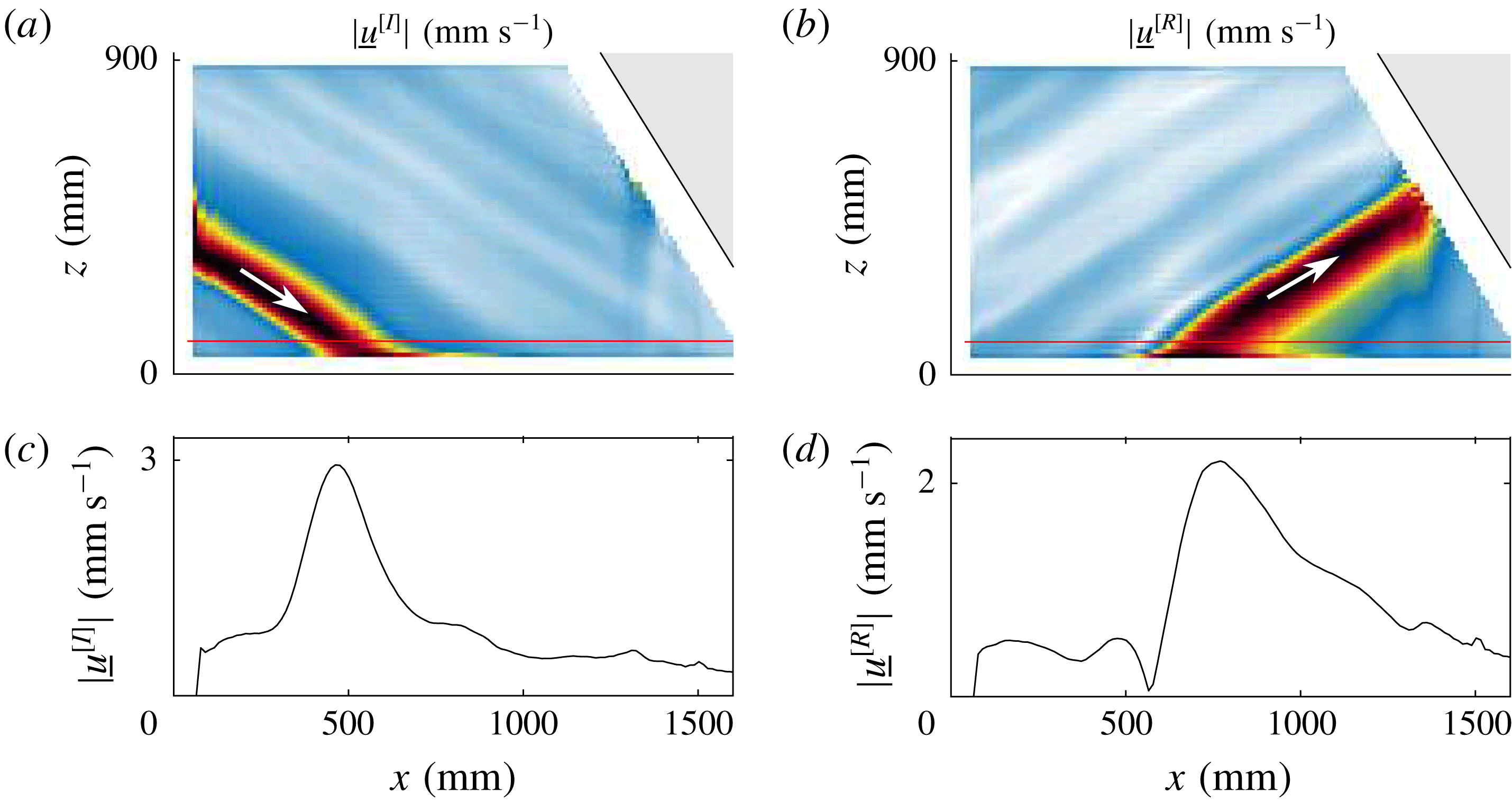
. Figure 6 shows an example of the incident and reflected beams, in the case of the bottom reflection. From this profile, we can compute
 $\langle p_{\bot }\rangle _{T_{0}}=\langle p_{\bot }^{[1]}\rangle _{T_{0}}+\langle p_{\bot }^{[3]}\rangle _{T_{0}}+\langle p_{\bot }^{[4]}\rangle _{T_{0}}$
using (3.29). As we will see in next section, this sum is of the same order of magnitude of the dissipation in the bulk and is ten times smaller than the dissipation taking place in the parallel boundary layers. This result is expected since the volume of the parallel boundary layers is much larger due to the small width of the tank. Varying
 $W$
clearly changes the importance of the parallel boundary layers compared to the perpendicular ones, as will be shown in § 4.3.
We will now apply these methods to measure the different terms in the energy budget for the attractors in several regimes.
Incident (a,c) and reflected (b,d) velocity amplitudes (a,b) along the direction of the bottom boundary, obtained at
 $t=50T_{0}$
thanks to Hilbert filtering. Panels (c,d) correspond to the horizontal cut at the altitude
 $z=100~\text{mm}$
shown in (a,b) by the red horizontal lines. Experimental parameters are those given in the caption of figure 2.

4 Results
4.1 Linear regime
To validate the quantitative estimation of the different terms of the energy balance, a complete analysis is performed for an attractor in the linear regime. This is done with a small forcing amplitude (
 $a_{0}=2~\text{mm}$
) using the following experimental scenario. The stratified fluid being initially at rest, the wavemaker is turned on at
 $t=0$
. After a few forcing periods
 $T_{0}$
, the injected energy rate becomes stationary as anticipated in figure 3(b). Finally, after
 $60T_{0}$
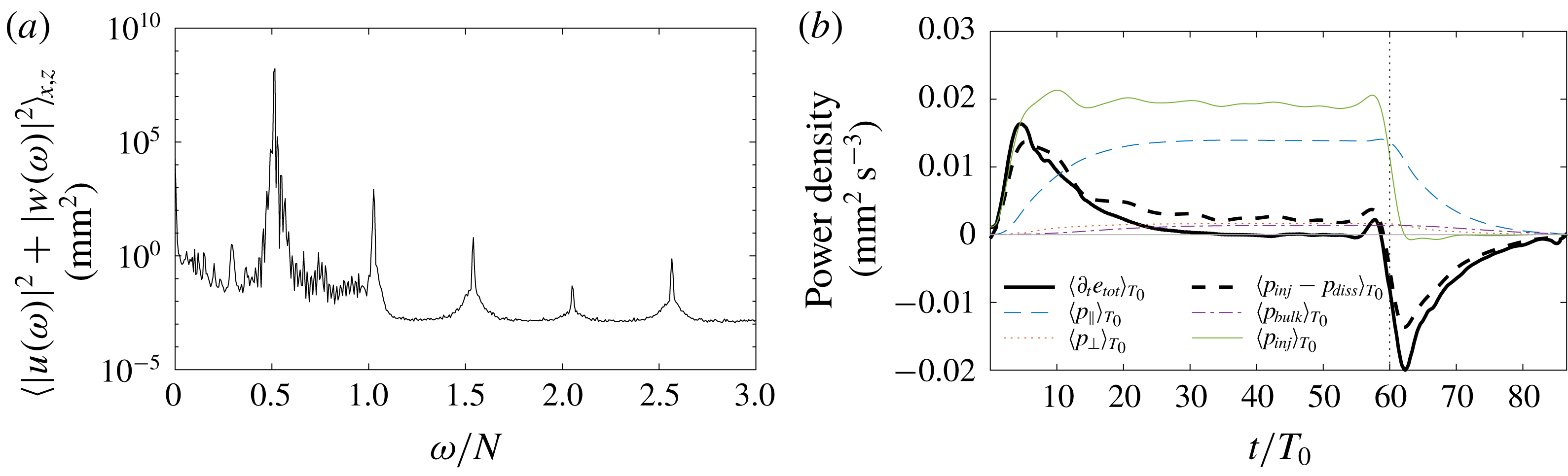
, the generator is turned off to observe the decay of the attractor. The power spectrum of the velocity field is displayed in figure 7(a). We see that most of the energy is located near the forcing frequency
 $\unicode[STIX]{x1D714}_{0}/N=0.52$
: the signal is then filtered around the forcing frequency to remove the external noise which could increase the errors in the estimation of the dissipative terms.
Figure 7(b) presents the time evolution of the different terms involved in the energy balance: the injected energy
 $p_{inj}$
and the three contributions of dissipation
 $p_{bulk}$
,
 $p_{\bot }$
and
 $p_{\Vert }$
. As mentioned in § 3.2.2,
 $p_{inj}$
is computed at
 $x_{0}\simeq 5~\text{cm}$
and therefore the dissipation occurring near the generator should not be taken into account. For this reason, we omit
 $p_{\bot }^{[3]}$
and correct
 $p_{bulk}$
and
 $p_{\Vert }$
accordingly. We see that the variations of the total energy are very well given by the difference of the injected power with the three dissipative terms. After approximately 30 periods, a steady state has been reached. Without any adjustable parameters, the difference between the estimated dissipation and injected power is then less than
 $10\,\%$
, showing therefore a good agreement within experimental errors. As emphasized by figure 7(b), this good agreement holds also in non-stationary situations, when we turn on or off the generator. Indeed, both curves have similar variations just after the switching times
 $t=$
0 and
 $60T_{0}$
, due to the changes in injected power. Notice that the fluctuations appearing on both curves just before
 $t=60T_{0}$
are due to the applied frequency filter, thus limiting sharp changes in the signals.
Similar experiments have been realized with larger amplitudes and therefore larger injected power. For each experiment, the signal is filtered around the forcing frequency
 $\unicode[STIX]{x1D714}_{0}$
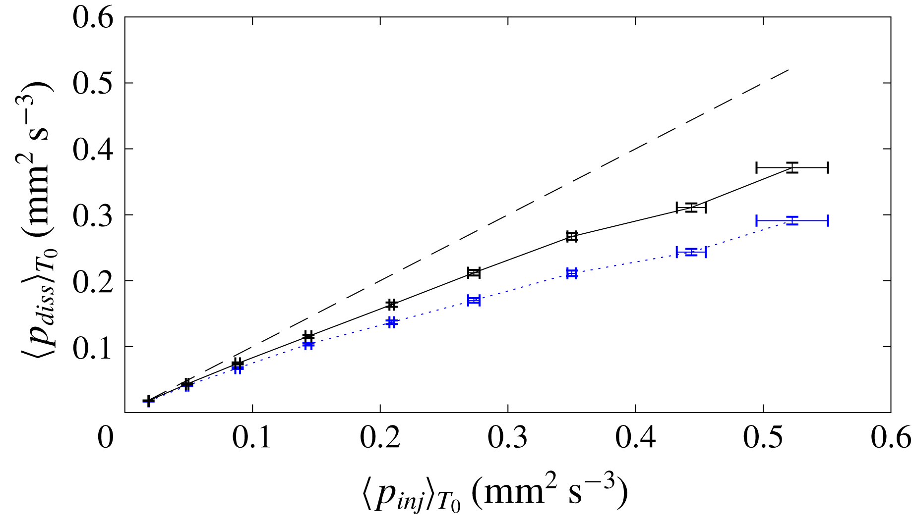
and the dissipation, measured in the steady state, is plotted as a function of the injected power in figure 8 (dotted line). The agreement is excellent at low amplitude but the deviation between the dissipation at
 $\unicode[STIX]{x1D714}_{0}$
and the injected power increases when considering larger amplitudes. This is expected since nonlinear effects can no longer be neglected: we have to consider other frequencies as discussed in the next subsection.
Linear regime. For both panels, experimental parameters are those given in the caption of figure 2 with a forcing amplitude
 $a_{0}=2~\text{mm}$
. (a) Power spectrum as a function of the frequency normalized by the buoyancy frequency
 $N$
(averaged over the area
 ${\mathcal{A}}$
and in logarithmic scale). Only waves with frequencies below this threshold value are propagating, but we clearly see several harmonics. (b) Evolution in time of the derivative of the total energy, the injected power and the different dissipative terms. The velocity field has been filtered around the forcing frequency
 $\unicode[STIX]{x1D714}_{0}$
before computing these quantities. Oscillations at
 $\unicode[STIX]{x1D714}_{0}$
have then been removed using a moving average based on their extrema. The generator has been switched on at
 $t=0$
and turned off at
 $t=60T_{0}$
, as emphasized by the vertical dotted line.

Full dissipation as a function of the measured injected power in the stationary regime. The blue dotted line corresponds to the velocity field filtered around the excitation frequency
 $\unicode[STIX]{x1D714}_{0}$
. The black line takes into account all frequencies below the buoyancy frequency
 $N$
. The
 $x$
-axis error bars are computed through the fluctuations of
 $\langle p_{inj}\rangle _{T_{0}}$
in time, while
 $y$
-axis error bars come from the uncertainty of the PIV measurement of velocity field. The dashed line corresponds to the expected relation
 $\langle p_{inj}\rangle _{T_{0}}=\langle p_{diss}\rangle _{T_{0}}$
.

4.2 Weakly nonlinear regime
By increasing the amplitude of the forcing, with values from
 $2$
to
 $10$
mm, the nonlinear regime is reached. As underlined by Brouzet et al. (Reference Brouzet, Ermanyuk, Joubaud, Sibgatullin and Dauxois2016a
), the set-up could model at large amplitude a cascade of triadic interactions transferring energy to different frequencies and smaller scales. For all amplitudes, a stationary state, defined as the absence of time variation of the total energy, is observed, meaning that the injected power is balanced by the dissipation.
We compute the different terms of (3.7) as we did in the linear case. The injected power is computed exactly in the same way, with a prior filtering of the velocity field at the forcing frequency. Indeed, since the generator oscillates exactly at
 $\unicode[STIX]{x1D714}_{0}$
, we have
 $p_{inj}(\unicode[STIX]{x1D714}\neq \unicode[STIX]{x1D714}_{0})=0$
, as verified experimentally. Some nonlinear corrections to the estimation of the pressure gradient have been computed and appear to be very small (less than 1 %). They are therefore neglected in the following. To evaluate the parallel dissipation
 $p_{\Vert }$
, a similar method than the one described in § 3.2.4 is used. To do so, we assume that the linear approximation used to obtain the velocity field in the boundary layer is still valid. Equations (3.22) and (3.23) are therefore multiplied by the time Fourier transform of the velocity field, low-pass filtered with a cutoff frequency equal to the buoyancy frequency
 $N$
. The real part of the inverse time Fourier transform of the obtained signal is finally used to get the value of
 $\unicode[STIX]{x2202}_{y}\boldsymbol{u}(x,z,t)$
and
 $p_{\Vert }$
in the boundary layers for all waves with frequency smaller than
 $N$
present in the domain.
As we showed that
 $p_{\bot }\simeq 0.1p_{\Vert }$
, we neglect the perpendicular dissipation due to the secondary waves, and we will consider
 $p_{\bot }\simeq p_{\bot }(\unicode[STIX]{x1D714}_{0})$
. On the contrary, as secondary waves usually present smaller length scales, we cannot a priori neglect their contribution to the bulk dissipation, which is measured here by computing (3.16) with only a band-pass filter to remove noise above the buoyancy frequency.
The black line of figure 8 shows, in the stationary regime, the dissipation measured in this way as a function of the injected power. The agreement with the expected relation
 $\langle p_{inj}\rangle =\langle p_{diss}\rangle _{T_{0}}$
represented by a dashed line has been significantly improved with respect to the one obtained when considering only the dissipation at
 $\unicode[STIX]{x1D714}_{0}$
. For very large amplitudes, the dissipation associated with the forcing
 $\unicode[STIX]{x1D714}_{0}$
represents only half of the injected power. Moreover, we have quantitatively shown that the secondary waves forced by successive triadic interactions represent approximately 16 % of the injected power in the strongest nonlinear regime.
To go into more detail, we will describe the time evolution of the different terms of the energy balance in the nonlinear regime. A typical power spectrum, for an intermediate forcing amplitude
 $a_{0}=5$
mm and an injected power of
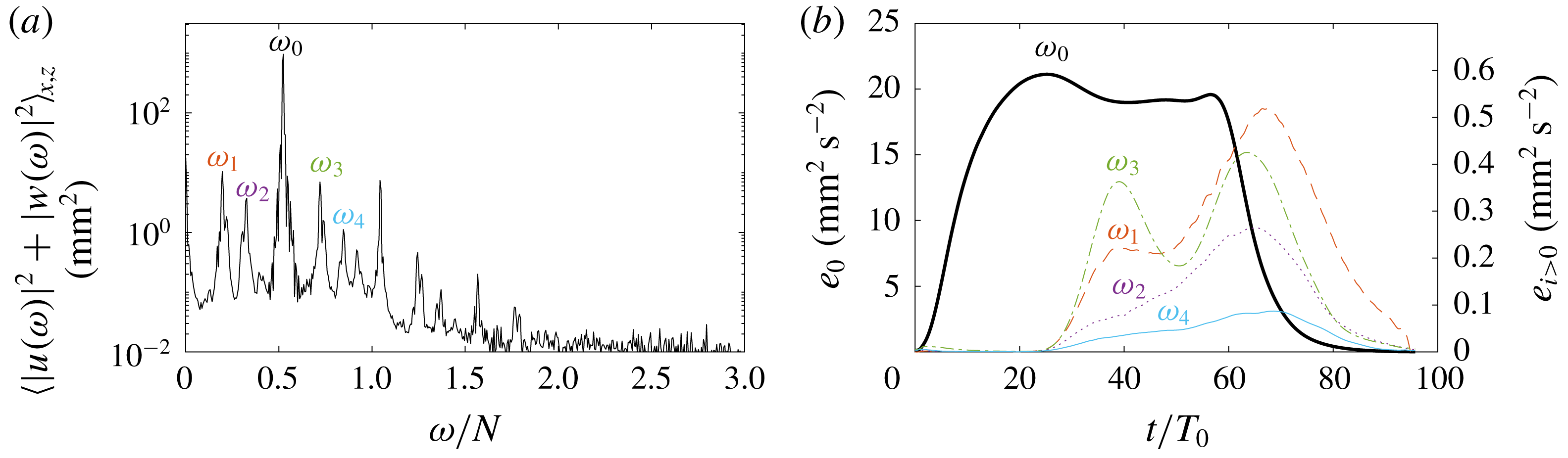
 $1.9\times 10^{-2}~\text{mm}^{2}~\text{s}^{-3}$
, is shown in figure 9(a). While the wave field is strongly dominated by the forcing frequency
 $\unicode[STIX]{x1D714}_{0}$
, we clearly see several other peaks. With this tool, one can investigate the exchange of energy between the different components of the velocity field. Figure 9(b) shows the evolution of the energies of the five most important components identified in figure 9(a). After the generator has been turned on at
 $t=0$
, the energy of the primary wave
 $\unicode[STIX]{x1D714}_{0}$
increases. Then, approximately
 $25$
periods later (corresponding to the typical time scale for the appearance of the triadic resonance interaction (TRI)), some energy loss of the primary wave is observed while the energy of the secondary waves increases, indicating an energy transfer. Some of them present some decrease of energy, which seems to show a complex interaction between the secondary waves. As can be seen in figure 8, the dissipation due to the primary wave slightly underestimates the injected power. For this weakly nonlinear case, the energy of the secondary waves is very small, and so is their dissipation. Even if it is of the same order of magnitude as the error bars, it seems that their presence explains the difference between the injected power and the dissipation due to the forcing frequency.
Weakly nonlinear regime. (a) Power spectrum as a function of the frequency normalized by the buoyancy frequency
 $N$
(averaged over the area
 ${\mathcal{A}}$
and in logarithmic scale). Experimental parameters are those given in the caption of figure 2 except
 $a_{0}=5~\text{mm}$
. The five main frequencies have been labelled
 $\unicode[STIX]{x1D714}_{i}$
with
 $i=0{-}4$
. (b) Evolution of the energy of the five main components of the velocity field. Note the difference in the energetic scale between the left
 $y$
-axis (corresponding to
 $e_{0}$
, the energy of the forcing frequency
 $\unicode[STIX]{x1D714}_{0}$
) and the right y-axis (corresponding to
 $e_{i}$
with
 $i>0$
for each
 $\unicode[STIX]{x1D714}_{i}$
). The generator is switched on at
 $t=0$
while turned off at
 $t=60T_{0}$
.

To confirm this hypothesis, we look in more detail at the case with the largest amplitude
 $a=10~\text{mm}$
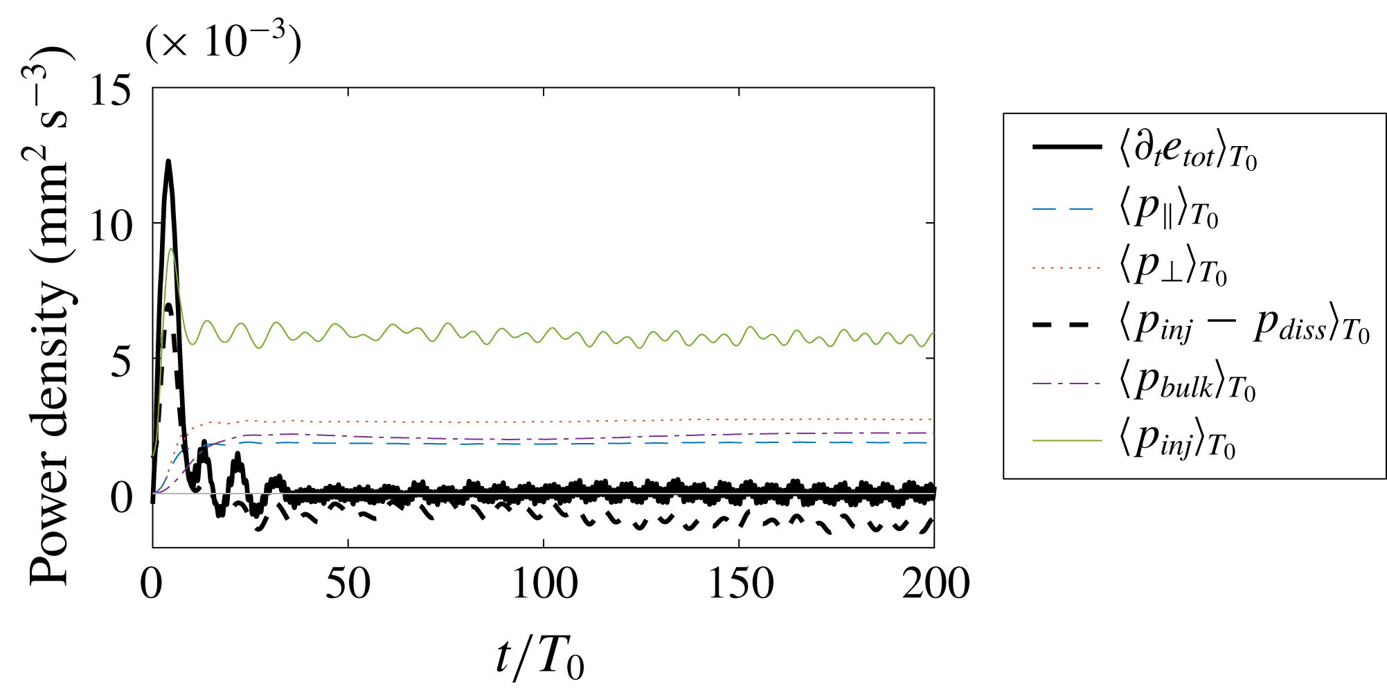
, which corresponds to a stronger nonlinear regime with a rich multi-peak spectrum. Figure 10 displays the time evolution of the different terms involved in the energy balance in which we have separated the dissipative part at the forcing frequency and the part due to the secondary waves. The agreement is very good at the beginning of the experiment just after switching on the generator. At about
 $20T_{0}$
, a stationary state is reached where the time derivative of the total energy
 $\unicode[STIX]{x2202}_{t}e_{tot}$
vanishes with some oscillations. At
 $15T_{0}$
, the dissipation due to the forcing frequency decreases and is substituted by dissipation due to secondary waves. The latter finally reaches
 $16\,\%$
of the injected power. It is important to note that the bulk dissipation for secondary waves constitutes
 $30$
% of total dissipation of secondary waves and is therefore much more important than for the primary wave, in which
 $p_{bulk}(\unicode[STIX]{x1D714}_{0})\approx 10\,\%p_{diss}(\unicode[STIX]{x1D714}_{0})$
. This result is expected since the typical length scales for the secondary waves are smaller. Even though the estimation of the dissipation due to the forcing frequency and the secondary waves gives an interesting estimation of the injected energy within the system, figures 8 and 10 show that the part of the dissipation not taken into account represents a quarter of the total dissipation. It is more important when nonlinearities are stronger. Different hypotheses may be given to explain this missing part in the dissipation. (i) In our model, we did not take into account frequencies larger than
 $N$
for all dissipation nor polychromaticity in the boundary layers when we estimated the perpendicular dissipation. The reflection at the free surface may also be the origin of some dissipation, since the boundary conditions is in reality between no slip and free slip due to surface contamination (Campagne et al.
Reference Campagne, Roumaissa, Redor, Sommeria, Valran, Viboud and Mordant2018). (ii) The average over the forcing period
 $T_{0}$
of some terms in (3.4) is not vanishing anymore in such a polychromatic case. (iii) The bulk dissipation may be underestimated. Indeed, the smallest scale we have access to is given by the resolution of the PIV measurements. Due to nonlinearities, some energy may be transferred to scales smaller than
 $10~\text{mm}$
and is not measured. (iv) Motions or dependence in the
 $y$
-direction are not taken into account. Secondary waves are assumed here to keep the two-dimensional geometry, which is not certain. (v) We see in figure 7 that some energy goes into a mean flow generated in the boundary layers (Horne et al.
Reference Horne, Beckebanze, Micard, Odier, Maas and Joubaud2019). While the associated dissipation in the bulk is taken into account, its counterpart in the boundary layers is not. (vi) Finally, part of the energy may be taken to increase the potential energy of the fluid, which is related to a homogenization of the density through mixing.
Nonlinear regime. Evolution in time of the derivative of the total energy
 $\unicode[STIX]{x2202}_{t}e_{tot}$
(thick black line), the injected power
 $p_{inj}$
(green solid line), the dissipation associated with the forcing frequency
 $p_{diss}(\unicode[STIX]{x1D714}_{0})$
(thin blue dashed line), the dissipation associated with other frequencies smaller than
 $N$
,
 $p_{diss}(\unicode[STIX]{x1D714}<N,\unicode[STIX]{x1D714}\neq \unicode[STIX]{x1D714}_{0})$
(blue dotted line) and finally the difference
 $p_{inj}-p_{diss}$
(thick black dashed line). Experimental parameters are those given in the caption of figure 2 except
 $a_{0}=10~\text{mm}$
.

4.3 Three-dimensional tank
As already underlined, the geometry of the domain has an effect on the importance of the different dissipative terms. Indeed, neglecting the feedback of the dissipation on the attractor, the bulk part as well as the perpendicular part depend linearly on the thickness of the tank, while the parallel part is independent of
 $W$
. To investigate a regime where dissipation is less dominated by the dissipation due to lateral walls, i.e. with a relatively lower
 $p_{\Vert }$
, we ran an experiment in a linear regime in a different tank of size
 $L\times W\times H=570\times 800\times 320~\text{mm}^{3}$
with a comparable slope of
 $\unicode[STIX]{x1D6FC}=29^{\circ }$
; the wavemaker is 150 mm wide. As shown in Pillet et al. (Reference Pillet, Ermanyuk, Maas, Sibgatullin and Dauxois2018) in which the details of the experimental set-up are given, the hypothesis of the two-dimensionality of the flow still holds in this tank within the linear and stationary regime. Note that the perpendicular dissipation
 $p_{\bot }^{[3]}$
on the left has now to be taken into account since the wavemaker does not occupy the total width of the tank. As shown in figure 11, we found that in this case the three dissipation rates are more comparable in magnitude, since
 $W$
is now
 $5$
times larger while
 $L$
and
 $H$
are both approximately 3 times smaller. The agreement between the measured quantities and the theory is again very good both in the non-stationary and the stationary regimes.
Evolution of the derivative of total energy, injected power and the different dissipative terms in time, for a linear experiment with forcing amplitude
 $a_{0}=5~\text{mm}$
in the three-dimensional tank. Note the
 $10^{-3}$
factor on the
 $y$
-axis. The field had been filtered around the forcing frequency before computing these quantities.

5 Conclusions
The goal of the work presented in this paper was to investigate the energy budget of a two-dimensional internal wave attractor using experiments. In the linear regime, we have shown that it is possible to simultaneously measure the energy flux injected into the system and the dissipation rate using two-dimensional, two-component PIV measurements. The pressure field, usually not accessible in laboratory or field measurements, is computed from the velocity field and gives access to the injected power
 $p_{inj}$
. The dissipation is disentangled into three different terms following the work of Beckebanze et al. (Reference Beckebanze, Brouzet, Sibgatullin and Maas2018): the bulk part is directly calculated from the velocity field, while the parallel and perpendicular parts due to the dissipation in the boundary layers, in the lateral walls and at the reflection of the internal wave beam, are quantified using a linear modelling of the boundary layer. We have shown that this procedure captures, without any adjustable parameters, the complete energy balance in the stationary state as well as in the transient regime.
Moreover, two different experimental set-ups have been used to quantify the importance of the parallel dissipation compared to the bulk dissipation. The ratio depends on the distance between the lateral walls and on the thickness of the boundary layers compared with the typical wavelength of the internal waves within the attractor. Using similar scaling arguments, the ratio between the bulk and the perpendicular dissipations depends on the thickness of the boundary layers and the typical size of the regions where a reflection occurs, which is close to the perimeter of the domain compared with the typical wavelength of the internal waves within the attractor.
Finally, we have shown that our analysis developed for the linear case is still valid in the nonlinear regime. Even if we cannot completely capture the total dissipation in the tank, we have quantified that the secondary waves generated through triadic resonant interactions clearly play a non-negligible role in the dissipation rate. As the difference between dissipation and variation of energy of a given component of the wave field gives access to its energy input, the analysis presented here could be part of the investigation of nonlinear energy transfers between different waves. It is also important to emphasize that the method tested here on internal wave attractors can be generalized straightforwardly to any quasi-two-dimensional stratified flow.
Acknowledgements
We thank E. Ermanyuk, B. Gallet and I. Sibgatullin for insightful discussions. This work was supported by the LABEX iMUST (ANR-10-LABX-0064) of Université de Lyon, within the programme ‘Investissements d’Avenir’ (ANR-11-IDEX-0007), operated by the French National Research Agency (ANR), France. This work has been supported by the ANR, France through grant ANR-17-CE30-0003 (DisET). This work has been achieved thanks to the resources of PSMN from ENS de Lyon.