1 Introduction
The intrinsic complexity of turbulence arising from the nonlinearity of the governing Navier–Stokes equations eludes an analytical description and requires experimental or advanced numerical tools to gain insight into the fundamental phenomena in such complex flows. Challenges for state-of-the-art numerical and experimental methods become even more apparent when various distinct flow features are combined and interact in a single flow field. Unfortunately, this is the case for almost all realistic applications and as a representative of such we consider in this paper the turbulent flow field in a valve/piston assembly during multiple cycles.
The main driving force of the flow field inside the chamber is given by the periodic motion of the piston inducing an unsteady turbulent flow with cyclic variability. During the intake stroke the piston draws fluid into the chamber, creating a hollow jet as the fluid is pushed through the valve. This results in the formation of large vortex structures, where the interaction with the cylinder walls causes a tumbling and swirling motion at larger scales. The hollow jet has similar flow features to a planar jet for which the turbulent flow field strongly depends on the distance to the nozzle. In first instance, a planar jet exhibits Kelvin–Helmholtz instabilities on both sides of the shear layers, eventually causing the jet breakup and the formation of small-scale turbulent structures (see, e.g., Gutmark & Wygnanski Reference Gutmark and Wygnanski1976; Stanley, Sarkar & Mellado Reference Stanley, Sarkar and Mellado2002; Mahesh Reference Mahesh2013). Note however, that the situation in the valve/piston arrangement is more intertwined as the large vortical structures, formed by the jet, are deflected by the cylinder walls and interact with the jet itself resulting in a different breakup behaviour. Furthermore, as for the planar jet, the breakup process, the spreading rate and the centre-line velocity are strongly influenced by the external flow field corresponding to the residual turbulence in the chamber at the beginning of a new cycle. This, in turn, alters the formation of the vortical structures and their influence on the jet breakup, leading to a cyclic variability (Schmitt et al. Reference Schmitt, Frouzakis, Wright, Tomboulides and Boulouchos2014b ). Cyclic variability is the consequence of the non-trivial interaction between small- and large-scale structures, which differs from most of the classical flows of fully developed turbulence for which the influence of the large-scale structures is more significant than vice versa. For the understanding of such complex phenomena numerical or experimental tools need to be applied.
Experimentally, an instantaneous, discrete velocity field may be obtained by techniques such as laser doppler velocimetry (LDV) or, more commonly, two- and three-dimensional particle image velocimetry (PIV). Despite substantial progress in this field, limitations in terms of temporal and spatial resolution become apparent considering the smallest scales. Nonetheless, valuable insight and validation data for numerical studies may be obtained from experiment. For instance, the experimental efforts of Morse, Whitelaw & Yianneskis (Reference Morse, Whitelaw and Yianneskis1979) using LDV in motored valve/piston assemblies are commonly used for validation of direct numerical simulations and turbulence models in this set-up. However, due to the limited access to the chamber, accurate measurements in the near-wall region are particularly challenging. For an overview of available experimental techniques we refer to the work of Towers & Towers (Reference Towers and Towers2008) and Westerweel, Elsinga & Adrian (Reference Westerweel, Elsinga and Adrian2013).
On the numerical side, direct numerical simulations (DNS), solving the Navier–Stokes equations directly and accounting for all pertinent scales of the flow, provide an accurate description of the flow field as no turbulence modelling, based on simplifying assumptions, is employed. However, for realistic applications of high Reynolds number flows involving complex geometries with moving boundaries such as the application considered in this paper, the computational cost becomes prohibitively high and only very few such simulations can be found in the literature. Most notable for this set-up is the recent DNS of Schmitt et al. (Reference Schmitt, Frouzakis, Tomboulides, Wright and Boulouchos2014a ) employing a high-order spectral element method and an arbitrary Lagrangian-Eulerian (ALE) formulation to account for the piston movement. In their work, a detailed analysis of the flow in the chamber with various velocity and stress profiles for different crank angles along with a quantification of cycle-to-cycle variability was presented. This gives us an opportunity to validate our simulations and study its behaviour in the case of under-resolution.
On the other hand, turbulence models reduce the computational requirements by not resolving all scales of the flow but by trying to account for the physical effects of the unresolved scales by projection onto the resolved ones. A prominent class, the so-called eddy-viscosity models, provides a closure to the coarse-grained Navier–Stokes equations by relating the Reynolds stress tensor to a turbulent eddy-viscosity
 ${\it\nu}_{t}$
. The intrinsic assumption behind the eddy-viscosity models is that the anisotropic part of the Reynolds stress tensor may be linearly related to the local mean rate-of-strain tensor via
 ${\it\nu}_{t}$
, analogous to the relation of the viscous stress in a Newtonian fluid. The analogy to the viscous stress is revealing as the comparison to kinetic theory and a simple time-scale analysis show that there is no general basis for either a local nor linear relationship between the rate-of-strain and the Reynolds stresses through a scalar quantity, see, e.g., Pope (Reference Pope2000) for telling examples. However, for simple cases, whenever the ratio of production to dissipation of turbulent kinetic energy is close to unity, the eddy-viscosity assumption holds with sufficient accuracy (Pope Reference Pope2000). In that context, various models prescribing the turbulent eddy-viscosity exist and range from algebraic relations to more sophisticated ones, solving a set of transport equations such as the
 $k-{\it\varepsilon}$
or
 $k-{\it\omega}$
models and their variants. Such models may be applied to either the Reynolds-averaged Navier–Stokes (RANS) equation or to the filtered Navier–Stokes equation yielding commonly used RANS and large-eddy simulation (LES) formulations, respectively. Despite the known deficiencies of the eddy-viscosity assumption as explained above, such models are often applied to various flows including the flow in the valve/piston assembly with its complex interaction of various base flow types, where the eddy-viscosity assumption is known to fail. In particular, these deficiencies have been assessed for strongly swirling flows, as often encountered in engine-type flows, in the work of Weber, Visser & Boysan (Reference Weber, Visser and Boysan1990). Still, due to their relatively low computational cost these models remain an attractive option to study turbulence phenomena. For the valve/piston assembly, LES has become increasingly popular as it overcomes the shortcomings of RANS, where a time or ensemble average is computed and cycle-specific phenomena as well as cyclic variability cannot be investigated. For an overview of RANS and LES applied to engine flows the reader is referred to the works of El Tahry & Haworth (Reference El Tahry and Haworth1992), Haworth (Reference Haworth1999), Celik, Yavuz & Smirnov (Reference Celik, Yavuz and Smirnov2001), Liu & Haworth (Reference Liu and Haworth2010) and Rutland (Reference Rutland2011). In particular, in Liu & Haworth (Reference Liu and Haworth2010), various LES models were tested and a reasonable agreement with experimental data was achieved, although it was pointed out that no model was capable of improving the comparison for all relevant quantities. An intrinsic issue of using such modelling approaches is that to date no universality exists and the model parameter specification is problem-dependent, typically only reliably available for simple, homogeneous turbulence with periodic boundaries. Furthermore, as most turbulence is generated in the near-wall region for wall-bounded flows, this issue needs to be addressed for turbulence models. As was stated in the recent review of Rutland (Reference Rutland2011), the development of wall models has made no significant progress in recent years. Hence, most LES need either to increase the resolution in the near-wall region (Kannepalli & Piomelli Reference Kannepalli and Piomelli2000) or are forced to overcome the stringent resolution requirement by employing wall functions based on the law of the wall (see Piomelli & Elias (Reference Piomelli and Elias2002) for a review on this topic in the LES context). Thus, the range of applicability of those models is limited and requires fine tuning of the model parameters for a specific set-up.
Lattice Boltzmann models
To overcome the high computational cost of DNS and to avoid the cumbersome search for the best tuning parameters in turbulence models, much research was focused on the development of accurate alternatives. To that end, the lattice Boltzmann (LB) method made significant progress, promising an efficient alternative with applications ranging from high Reynolds number flows (Chen et al.
Reference Chen, Kandasamy, Orszag, Shock, Succi and Yakhot2003; Thantanapally et al.
Reference Thantanapally, Singh, Patil, Succi and Ansumali2013; Karlin, Bösch & Chikatamarla Reference Karlin, Bösch and Chikatamarla2014), multiphase flows (Mazloomi, Chikatamarla & Karlin Reference Mazloomi, Chikatamarla and Karlin2015), thermal flows (Frapolli, Chikatamarla & Karlin Reference Frapolli, Chikatamarla and Karlin2014) to relativistic hydrodynamics (Mendoza et al.
Reference Mendoza, Boghosian, Herrmann and Succi2010). By employing kinetic theory, the lattice Boltzmann method (LBM) describes the flow field in terms of discretized particle distribution functions (populations)
 $f_{i}(\boldsymbol{x},t)$
associated with discrete velocities
 $\boldsymbol{c}_{i},i=1,\ldots ,Q$
, designed to recover the macroscopic Navier–Stokes equations in the hydrodynamic limit (see, e.g., Succi Reference Succi2001). By fitting the discrete velocities into a regular lattice, a simple and highly efficient stream-and-collide algorithm with exact propagation is realized, for which the nonlinearity is local in space. Apart from the popular Bhatnagar–Gross–Krook lattice Boltzmann model (LBGK), various LB models have been developed in recent years, which differ in the realization of the collision operator. However, despite its efficiency and simplicity, the success for the LBM was limited to resolved, moderate Reynolds number flows due to the lack of numerical stability in under-resolved simulations. On one hand, this promoted the development of turbulence models such as systematic renormalization group-based
 $k-{\it\varepsilon}$
eddy-viscosity models (see Chen et al.
Reference Chen, Kandasamy, Orszag, Shock, Succi and Yakhot2003), where an effective relaxation time can be derived in Fourier and real spaces. This has been successfully applied to high Reynolds number flows, analogous to conventional turbulence models as described above. Further, in the field of internal combustion engines notable modelling approaches on spray formation, breakup and cavitation in the LB realm are given in the works of Falcucci et al. (Reference Falcucci, Ubertini, Bella, De Maio and Palpacelli2010, Reference Falcucci, Jannelli, Ubertini and Succi2013). On the other hand, the stability issue has been overcome by Karlin, Ferrante & Öttinger (Reference Karlin, Ferrante and Öttinger1999) by introducing the discrete entropy function as the determining factor of the relaxation, chosen to obey the second law of thermodynamics and thus yielding the nonlinearly stable entropic lattice Boltzmann method (ELBM). In contrast to LBGK, the ELBM chooses the relaxation parameter of the collision adaptively at each point in space and time to locally ensure the discrete-time H-theorem. The macroscopic effect of choosing the relaxation parameter in this manner results in a locally varying, effective viscosity, which can be larger or smaller than the nominal one, leading to local enhancement or smoothing of the flow field (Karlin et al.
Reference Karlin, Ansumali, De Angelis, Öttinger and Succi2003). This originates from the fact that, in ELBM, the same relaxation is equivalently imposed on all moments of the populations beyond the locally conserved quantities. It is important to stress that the relaxation parameter is not arbitrarily chosen but rather dictated by the physics of the flow, in accordance with the second law of thermodynamics. However, for resolved simulations where the populations remain close to the equilibrium state, the ELBM recovers the LBGK model with its nominal viscosity (Karlin, Succi & Chikatamarla Reference Karlin, Succi and Chikatamarla2011).
An extension of the entropy concept was recently proposed by Karlin et al. (Reference Karlin, Bösch and Chikatamarla2014), where the viscosity may be kept at its nominal value by considering multiple relaxation times (Karlin–Bösch–Chikatamarla (KBC) models). Recent studies of Bösch, Chikatamarla & Karlin (Reference Bösch, Chikatamarla and Karlin2015) have shown outstanding numerical stability for high Reynolds number flows while accuracy was not sacrificed. Furthermore, the role of the entropic stabilizer was investigated and quantified for periodic turbulence (Bösch et al. Reference Bösch, Chikatamarla and Karlin2015). In this paper, we go beyond the periodic set-up and study the subgrid features of KBC models in the valve/piston assembly. With the recent development of stable and accurate boundary conditions (Dorschner et al. Reference Dorschner, Chikatamarla, Bösch and Karlin2015), the implementation of complex geometries with moving boundaries comes at little additional cost. Our results indicate that the KBC model provides a simple and efficient alternative to conventional CFD methods for research and engineering applications.
The outline of the paper is as follows. In § 2, a brief review of KBC models and boundary conditions is presented. Before considering the full complexity of the valve/piston assembly, § 3 presents a validation of simple flows such as the Kida vortex flow and the turbulent pipe flow using the KBC model with an emphasis on coarse-resolution simulations. Finally, § 4 discusses the valve/piston assembly by a comparison of our simulation results with state-of-the-art DNS and the experimental data of Morse et al. (Reference Morse, Whitelaw and Yianneskis1979) and Schmitt et al. (Reference Schmitt, Frouzakis, Tomboulides, Wright and Boulouchos2014a ), respectively. As in § 3, the KBC model’s subgrid behaviour is tested numerically for various resolutions.
2 Entropic multi-relaxation time lattice Boltzmann models
The evolution of the population
 $f_{i}$
is given by the discrete kinetic equation
 $$\begin{eqnarray}\displaystyle f_{i}(\boldsymbol{x}+\boldsymbol{c}_{i},t+1)=f_{i}^{\prime }=(1-{\it\beta})f_{i}(\boldsymbol{x},t)+{\it\beta}f_{i}^{mirr}(\boldsymbol{x},t), & & \displaystyle\end{eqnarray}$$
where the advection is accounted for by the left-hand side and the post-collision state
 $f_{i}^{\prime }$
is represented on the right-hand side by a convex linear combination between the population
 $f_{i}(\boldsymbol{x},t)$
and the maximally over-relaxed mirror state
 $f_{i}^{mirr}(\boldsymbol{x},t)$
; the parameter
 ${\it\beta}$
is related to the kinematic viscosity. Note that all lattice Boltzmann models differ only in the realization of the mirror state and the classical LBGK model defines it as
 $$\begin{eqnarray}\displaystyle f_{i}^{mirr}(\boldsymbol{x},t)=2f_{i}^{eq}-f_{i}, & & \displaystyle\end{eqnarray}$$
where the equilibrium
 $f_{i}^{eq}$
is obtained by minimizing the discrete entropy function
 $H$
subject to the local conservation laws (density
 ${\it\rho}$
and momentum density
 $\boldsymbol{j}$
as given by the first two moments of the discrete distribution)
 $$\begin{eqnarray}\displaystyle \min \left\{H(f)=\mathop{\sum }_{i}f_{i}\ln \left(\frac{f_{i}}{W_{i}}\right)\right\},\quad \text{s.t.}~\mathop{\sum }_{i}\{1,\boldsymbol{c}_{i}\}\,f_{i}=\{{\it\rho},\boldsymbol{j}\}. & & \displaystyle\end{eqnarray}$$
Here
 $W_{i}$
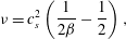
are the lattice specific weights. Using standard procedures, it can be shown that the LBGK models in combination with a properly chosen lattice recover the Navier–Stokes equations in the hydrodynamic limit with the kinematic viscosity
 $$\begin{eqnarray}\displaystyle {\it\nu}=c_{s}^{2}\left(\frac{1}{2{\it\beta}}-\frac{1}{2}\right), & & \displaystyle\end{eqnarray}$$
where
 $c_{s}$
denotes the speed of sound, defined by the lattice of choice. In this paper, the standard
 $D3Q27$
-lattice (dimensionality
 $D=3$
, number of discrete velocities
 $Q=27$
) is used for all computations, where the speed of sound amounts to
 $c_{s}=1/\sqrt{3}$
. The exact entropic equilibrium on this lattice can be found in Ansumali, Karlin & Öttinger (Reference Ansumali, Karlin and Öttinger2003).
Going beyond the single-relaxation time LBGK model, which is limited to fully resolved, moderate Reynolds number flow simulations, multi-relaxation time (MRT) models are considered next. MRT models exploit the fact that the dimensionality of the kinetic system is typically much larger than required to recover the Navier–Stokes equation in the hydrodynamic limit. Thus, the non-hydrodynamic, higher-order moments are relaxed independently aiming to increase stability. At which rate these moments are relaxed is a priori not clear and requires flow-dependent fine tuning (Lallemand & Luo Reference Lallemand and Luo2000; Geier, Greiner & Korvink Reference Geier, Greiner and Korvink2006). This issue was resolved in the work of Karlin et al. (Reference Karlin, Bösch and Chikatamarla2014) by the introduction of KBC models.
Let us recall that the set of natural moments of the
 $D3Q27$
-lattice is given by
 $$\begin{eqnarray}\displaystyle {\it\rho}M_{pqr}=\mathop{\sum }_{i}f_{i}c_{ix}^{p}c_{iy}^{q}c_{iz}^{r}\quad p,q,r\in \left\{0,1,2\right\}\!, & & \displaystyle\end{eqnarray}$$
yielding the conservation laws as the first
 $1+D$
moments and the pressure tensor
 $\boldsymbol{{\it\Pi}}$
as the second-order moments. Higher-order moments lack a direct physical interpretation in the athermal case.
This moment representation spans a basis in which a population can equivalently be expressed (see appendix A for the explicit expressions). Note that the moment basis is not unique and, for example, a central moment basis can be applied analogously (Bösch et al.
Reference Bösch, Chikatamarla and Karlin2015). With the moment representation, the population
 $f_{i}$
may be decomposed into three parts as
 $$\begin{eqnarray}\displaystyle f_{i}=k_{i}+s_{i}+h_{i}, & & \displaystyle\end{eqnarray}$$
where
 $k_{i}$
indicates the kinematic part and depends only on the conserved quantities. The shear part is denoted by
 $s_{i}$
and necessarily includes the deviatoric stress tensor
 $\boldsymbol{{\it\Pi}}^{\prime }=\boldsymbol{{\it\Pi}}-D^{-1}Tr(\boldsymbol{{\it\Pi}})\unicode[STIX]{x1D644}$
. Further non-conserved moments may however be included in
 $s_{i}$
, yielding a family of KBC models. The higher-order moments correspond to
 $h_{i}$
, which contains all remaining moments that are not included in
 $k_{i}$
or
 $s_{i}$
. Using this decomposition, the mirror state can be expressed as
 $$\begin{eqnarray}\displaystyle f_{i}^{mirr}=k_{i}+(2s_{i}^{eq}-s_{i})+((1-{\it\gamma})h_{i}+{\it\gamma}h_{i}^{eq}), & & \displaystyle\end{eqnarray}$$
where
 $s_{i}^{eq}$
and
 $h_{i}^{eq}$
indicate
 $s_{i}$
and
 $h_{i}$
evaluated at equilibrium and the parameter
 ${\it\gamma}$
is the relaxation rate of the higher-order moments. Note that any specification of
 ${\it\gamma}$
recovers the Navier–Stokes equation with the shear viscosity as given by (2.4) and the special case of
 ${\it\gamma}=2$
results in the LBGK model.
In this paper, we choose the shear part
 $s_{i}$
to include only the mandatory deviatoric stress
 $\boldsymbol{{\it\Pi}}^{\prime }$
and lump all other moments in
 $h_{i}$
(see, e.g., Bösch et al. (Reference Bösch, Chikatamarla and Karlin2015) for a thorough study of various KBC realizations), yielding the macroscopic equations as obtained through the standard Chapman–Enskog analysis as
 $$\begin{eqnarray}\displaystyle \partial _{t}{\it\rho} & = & \displaystyle -\boldsymbol{{\rm\nabla}}\boldsymbol{\cdot }({\it\rho}\boldsymbol{u}),\end{eqnarray}$$
 $$\begin{eqnarray}\displaystyle \partial _{t}\boldsymbol{u} & = & \displaystyle -\boldsymbol{u}\boldsymbol{\cdot }\boldsymbol{{\rm\nabla}}\boldsymbol{u}-{\it\rho}^{-1}\boldsymbol{{\rm\nabla}}p\nonumber\\ \displaystyle & & \displaystyle +\,{\it\rho}^{-1}\boldsymbol{{\rm\nabla}}\boldsymbol{\cdot }[{\it\nu}{\it\rho}(\boldsymbol{{\rm\nabla}}\boldsymbol{u}+\boldsymbol{{\rm\nabla}}\boldsymbol{u}^{\dagger }-2D^{-1}\unicode[STIX]{x1D644}\boldsymbol{{\rm\nabla}}\boldsymbol{\cdot }\boldsymbol{u})]+2D^{-1}{\it\rho}^{-1}\boldsymbol{{\rm\nabla}}[{\it\xi}{\it\rho}\boldsymbol{{\rm\nabla}}\boldsymbol{\cdot }\boldsymbol{u}],\end{eqnarray}$$
where the pressure is given by
 $p=c_{s}^{2}{\it\rho}$
. It is important to notice that the bulk viscosity for the present KBC model (only the deviatoric stress tensor is included in
 $s_{i}$
) is related to the parameter
 ${\it\gamma}$
as
 $$\begin{eqnarray}\displaystyle {\it\xi}=c_{s}^{2}\left(\frac{1}{{\it\gamma}{\it\beta}}-\frac{1}{2}\right). & & \displaystyle\end{eqnarray}$$
This is not the case if the shear part
 $s_{i}$
additionally includes
 $\text{Tr}\left(\boldsymbol{{\it\Pi}}\right)$
, leading to
 ${\it\xi}={\it\nu}$
. The main idea of KBC lies now in the specification of
 ${\it\gamma}$
, which is not tuned as in various other MRT models but rather computed locally in every time step and at every grid point by minimizing the discrete entropy function (see (2.3)) in the post-collision state
 $f_{i}^{\prime }$
. Carrying out the optimization leads to the following condition for
 ${\it\gamma}$
,
 $$\begin{eqnarray}\displaystyle \mathop{\sum }_{i}{\rm\Delta}h_{i}\ln \left[1+\frac{(1-{\it\beta}{\it\gamma}){\rm\Delta}h_{i}-(2{\it\beta}-1){\rm\Delta}s_{i}}{f_{i}^{eq}}\right]=0, & & \displaystyle\end{eqnarray}$$
where
 ${\rm\Delta}s_{i}=s_{i}-s_{i}^{eq}$
and
 ${\rm\Delta}h_{i}=h_{i}-h_{i}^{eq}$
denote the deviations from equilibrium. By introducing the entropic scalar product as
 $\langle X|Y\rangle =\sum _{i}(X_{i}Y_{i}/f_{i}^{eq})$
and an expansion of (2.11) to the first non-vanishing order of
 ${\rm\Delta}s_{i}/f_{i}^{eq}$
and
 ${\rm\Delta}h_{i}/f_{i}^{eq}$
, an analytic approximation for the relaxation parameter
 ${\it\gamma}$
may be found as
 $$\begin{eqnarray}\displaystyle {\it\gamma}=\frac{1}{{\it\beta}}-\left(2-\frac{1}{{\it\beta}}\right)\frac{\langle {\rm\Delta}s\mid {\rm\Delta}h\rangle }{\langle {\rm\Delta}h\mid {\rm\Delta}h\rangle }. & & \displaystyle\end{eqnarray}$$
This approximation has proven to be sufficient for all tested cases.
2.1 Wall-boundary conditions
As our study focuses on a geometry-driven flow, we shall briefly review the topic of wall-boundary conditions. In order to complete the advection step of the LB algorithm, the set of populations
 $\bar{D}$
advected from the solid into the fluid region are unknown and need to be specified. To that end, a variety of realizations can be found in the literature ranging from simple bounce-back boundary conditions using a crude staircase approximation to more sophisticated formulations trying to incorporate the curvature of the object. It is clear that for under-resolved simulations, the staircase approximation is not the best option as the geometry is not accurately represented. For curved boundary conditions, a common approach is to employ interpolation or extrapolation schemes onto the populations (see, e.g., Guo, Zheng & Shi Reference Guo, Zheng and Shi2002; Lallemand & Luo Reference Lallemand and Luo2003; Wang et al.
Reference Wang, Shu, Teo and Wu2015). However, their usage is limited to low Reynolds number flows as spurious shocks are triggered at the boundary for turbulence simulations (Lammers et al.
Reference Lammers, Beronov, Volkert, Brenner and Durst2006; Spasov, Rempfer & Mokhasi Reference Spasov, Rempfer and Mokhasi2009).
An alternative, recently proposed by Dorschner et al. (Reference Dorschner, Chikatamarla, Bösch and Karlin2015), is to impose the boundary conditions not on the highly fluctuating populations directly but rather on the slow varying moments, namely density, momentum and pressure. Here, the missing populations are approximated by an analogue of Grad’s distribution function, which results in a parametrization of the distribution in terms of relevant moments, including not only locally conserved quantities but also other pertinent moments. A derivation using maximum entropy or quasi-equilibrium considerations may be found in the work of Gorban & Karlin (Reference Gorban and Karlin2004). In the athermal case, it is sufficient to include the pressure tensor
 $\boldsymbol{{\it\Pi}}$
besides the conserved quantities, yielding
 $$\begin{eqnarray}\displaystyle f_{i}^{\ast }({\it\rho},\boldsymbol{u},\boldsymbol{{\it\Pi}})=W_{i}\left[{\it\rho}+\frac{{\it\rho}}{c_{s}^{2}}\boldsymbol{c}_{i}\boldsymbol{\cdot }\boldsymbol{u}+\frac{1}{2c_{s}^{4}}\left(\boldsymbol{{\it\Pi}}-{\it\rho}c_{s}^{2}\unicode[STIX]{x1D644}\right)\boldsymbol{ : }(\boldsymbol{c}_{i}\otimes \boldsymbol{c}_{i}-c_{s}^{2}\unicode[STIX]{x1D644})\right], & & \displaystyle\end{eqnarray}$$
where the pressure tensor
 $\boldsymbol{{\it\Pi}}$
is approximated by
 $$\begin{eqnarray}\displaystyle \boldsymbol{{\it\Pi}}=\boldsymbol{{\it\Pi}}^{eq}+\boldsymbol{{\it\Pi}}^{neq}, & & \displaystyle\end{eqnarray}$$
with
 $$\begin{eqnarray}\displaystyle & \displaystyle \boldsymbol{{\it\Pi}}^{eq}={\it\rho}c_{s}^{2}\unicode[STIX]{x1D644}+{\it\rho}\boldsymbol{u}\otimes \boldsymbol{u}, & \displaystyle\end{eqnarray}$$
 $$\begin{eqnarray}\displaystyle & \displaystyle \boldsymbol{{\it\Pi}}^{neq}=-\frac{{\it\rho}c_{s}^{2}}{2{\it\beta}}(\boldsymbol{{\rm\nabla}}\boldsymbol{u}+\boldsymbol{{\rm\nabla}}\boldsymbol{u}^{\dagger }). & \displaystyle\end{eqnarray}$$
The macroscopic variables to be used in
 $f_{i}^{\ast }$
(2.13) are specified by introducing the concept of target values. The target velocity is obtained using an interpolation scheme including the wall velocity and the velocity at the neighbouring fluid nodes. The target density is evaluated based on the bounce-back density. An additional term needs to be included into the target density in the case of a moving wall to account for the mass swept by the obstacle moving with the velocity
 $\boldsymbol{u}_{w}$
. This may be derived by introducing a forcing term necessary for the displacement and amounts to
 $$\begin{eqnarray}\displaystyle {\it\rho}_{dyn}=\mathop{\sum }_{i\in \bar{D}}6W_{i}{\it\rho}\boldsymbol{c}_{i}\boldsymbol{\cdot }\boldsymbol{u}_{w,i}. & & \displaystyle\end{eqnarray}$$
Finally, the pressure tensor is determined using a finite difference scheme for
 $\boldsymbol{{\rm\nabla}}\boldsymbol{u}$
and the velocity values from the previous time step. Note that for a moving object lattice sites are uncovered as the object passes by and require a reinitialization of the corresponding populations. In this case, we use the equilibrium distribution with the wall-velocity and a local density average. It needs to be mentioned that the wall-velocity may not be too large compared to the speed of sound
 $c_{s}$
. As shown in Dorschner et al. (Reference Dorschner, Chikatamarla, Bösch and Karlin2015), this yields a boundary condition compatible with the entropic considerations and thus the KBC model, where the stability issues of previously proposed schemes are resolved and second-order accuracy is retained. An extended discussion on the boundary conditions including all technical details is given in appendix B.
3 Model validation for simple flows
The valve/piston assembly reveals a number of hydrodynamic features typical for complex flows. Interactions between large-scale coherent structures which are perturbed by residual turbulence characterize the flow in the bulk of the chamber while the complex valve/cylinder geometry adds effects of wall-bounded flows. Moreover, the moving piston introduces yet another conceptual dimension to the problem. Not surprisingly, this variety of physically distinct flow patterns and complex nonlinear interactions among them introduce numerical challenges.
In order to show that the KBC model is capable of correctly predicting the physics of the main active flow regimes we consider a number of precursor simulations using the KBC model and boundary conditions as described in the previous section. By reducing the complexity of the flow and concentrating on a single flow regime we demonstrate that the method is able to accurately capture the main physics at hand individually. Thus, we conceptually decompose the problem into its building blocks while combining them in a last step. In particular, we put emphasis on the performance of the model in situations where the simulation cannot resolve all pertinent scales of the flow. Thereby, one can gain insight into the built-in subgrid features that the model exposes.
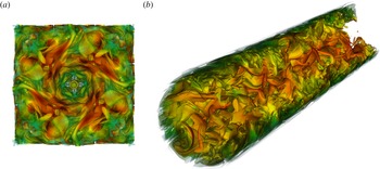
(a) Vortex structures for the periodic Kida vortex flow at
 $Re=6000$
(
 $x,y,z\in [0,{\rm\pi}]$
). (b) Turbulent pipe flow at
 $R^{+}=180$
visualized by iso-surfaces of vorticity magnitude coloured with velocity magnitude.

3.1 Turbulence in a periodic box
As the main flow in the bulk of the engine-like assembly is driven by vortex–vortex interaction and small-scale turbulence, we consider the Kida vortex flow as a classical benchmark simulation (see figure 1 a). This well-studied flow evolves from a deterministic and symmetric initial condition to a state that resembles a fully developed turbulent flow featuring a corresponding energy cascade and has been analysed extensively using DNS (Kida Reference Kida1985; Kida & Murakami Reference Kida and Murakami1987; Keating et al. Reference Keating, Vahala, Yepez, Soe and Vahala2007; Chikatamarla et al. Reference Chikatamarla, Frouzakis, Karlin, Tomboulides and Boulouchos2010). The initial conditions are given by
 $$\begin{eqnarray}\displaystyle \begin{array}{@{}rcl@{}}u_{x}(x,y,z)\; & =\; & U_{0}\sin x(\cos 3y\cos z-\cos y\cos 3z),\\ u_{y}(x,y,z)\; & =\; & U_{0}\sin y(\cos 3z\cos x-\cos z\cos 3x),\\ u_{z}(x,y,z)\; & =\; & U_{0}\sin z(\cos 3x\cos y-\cos x\cos 3y),\end{array} & & \displaystyle\end{eqnarray}$$
where
 $x,y,z\in [0,2{\rm\pi}]$
and periodic boundary conditions are imposed in all directions. The Reynolds number is defined as
 $Re=U_{0}N/{\it\nu}$
where
 $N$
is the domain size. While the kinetic energy is decaying, the evolution of enstrophy shows a steep increase in the early stage of the simulation and reaches a maximum value before it starts to decay. Just after the peak of enstrophy the flow reaches the most turbulent state producing large gradients and small-scale structures. While large gradients on the one hand may cause numerical instabilities, it is of paramount interest not to over-damp the dynamics on the other hand, which will lead to a corrupted and non-physical result lacking the small scales. Without employing explicit turbulence models one is usually restricted to increasing the resolution such that the smallest eddies are resolved. This is typically satisfied when the grid spacing is smaller than the Kolmogorov scale
 ${\it\eta}=({\it\nu}^{3}/{\it\epsilon})^{1/4}$
with kinematic viscosity
 ${\it\nu}$
and rate of energy dissipation
 ${\it\epsilon}$
.
In order to study the accuracy of the KBC model, a detailed investigation was recently conducted by Bösch et al. (Reference Bösch, Chikatamarla and Karlin2015). The Reynolds number here is
 $Re=6000$
, which is slightly higher than what can be expected for the valve/piston assembly considering the cylinder diameter and the maximum piston velocity as characteristic scales. A sufficiently resolved reference simulation (
 ${\it\eta}\approx 1.2~{\rm\Delta}x$
) is conducted with a box length of
 $N=600$
using the LBGK collision model. Further simulations with
 $N=\{100,200,400\}$
and the same Reynolds number using the KBC model are the carried out and compared to both the reference solution and theoretical limits (see Bösch et al.
Reference Bösch, Chikatamarla and Karlin2015).
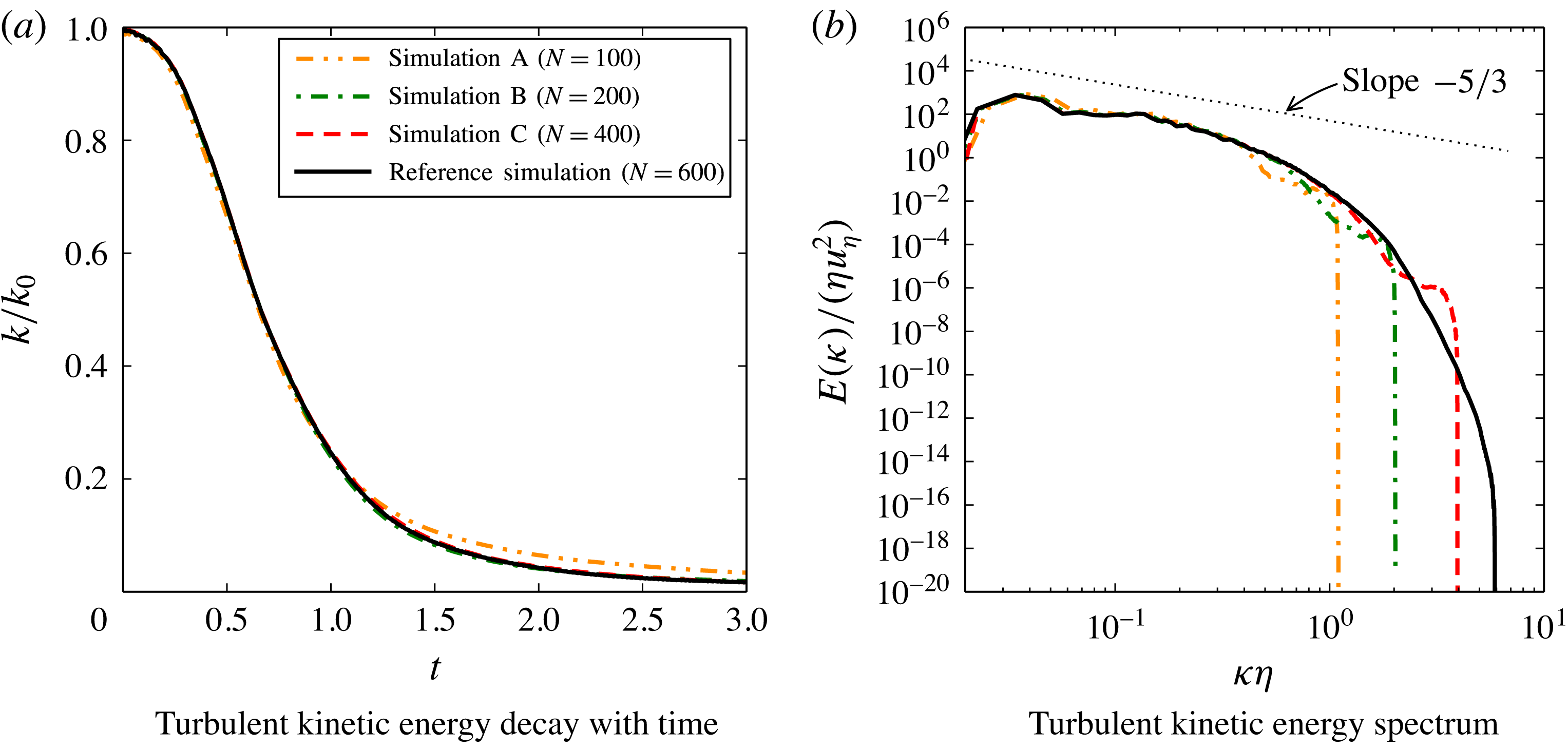
Statistics for the Kida vortex flow at
 $Re=6000$
and resolutions of
 $N=\{100,200,400\}$
and
 $N=600$
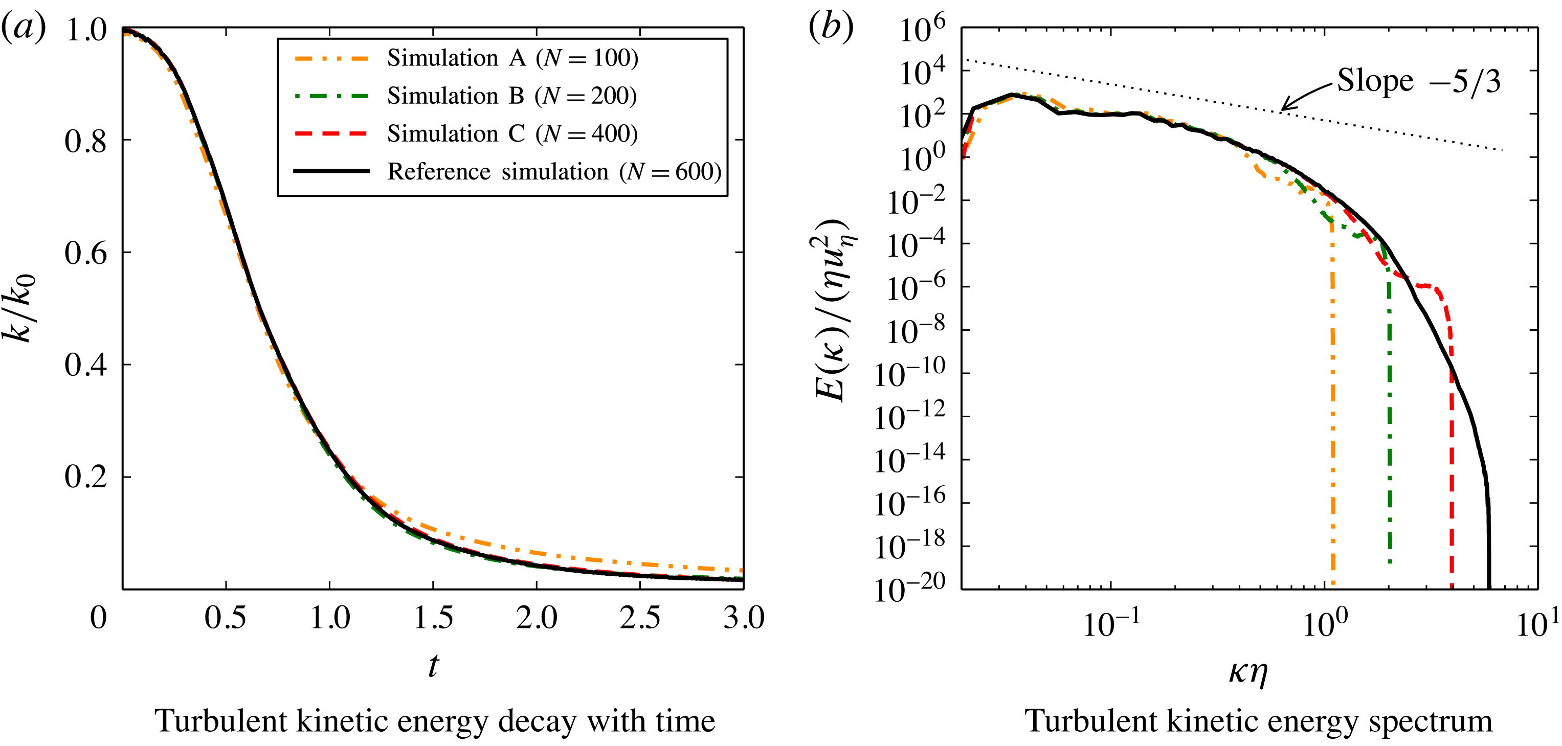
for the simulations with KBC and the reference simulation with LBGK, respectively. The theoretical Kolmogorov scaling is indicated by the dotted line.
An important global characteristic is the evolution of the turbulent kinetic energy
 $k$
as shown in figure 2(a). For all resolutions in this study the energy decay seems to be captured well despite the rather severe under-resolution in the coarsest simulation (
 ${\it\eta}\approx 0.2~{\rm\Delta}x$
). However, a more meaningful insight is given by the energy distribution across the scales of the flow as shown by means of the normalized energy spectrum along with the theoretical Kolmogorov scaling with a slope of
 $-5/3$
in the inertial subrange in figure 2(b). It is apparent that the energy scales with marginal difference for all resolutions with a sharp cut-off at its smallest scale as expected for a well-behaved subgrid model.
A thorough convergence study of various statistical quantities sampled at time points around the peak of enstrophy demonstrates second-order accuracy (see Bösch et al. Reference Bösch, Chikatamarla and Karlin2015) as is expected for a lattice Boltzmann method.
While convergence towards the reference solution is established, it is of interest to quantify the recovery of the Navier–Stokes equations at small scales. To that end, let us remind the reader that the incompressible Navier–Stokes equation implies the following balance equations for the averaged momentum, vorticity, energy and enstrophy which yield for statistically homogeneous flows (Lamb Reference Lamb1932; Batchelor Reference Batchelor2000),
 $$\begin{eqnarray}\displaystyle & \displaystyle \partial _{t}\langle \boldsymbol{u}\rangle =0, & \displaystyle\end{eqnarray}$$
 $$\begin{eqnarray}\displaystyle & \displaystyle \partial _{t}\langle {\bf\omega}\rangle =0, & \displaystyle\end{eqnarray}$$
 $$\begin{eqnarray}\displaystyle & \displaystyle \partial _{t}k=-2{\it\nu}{\it\Omega}, & \displaystyle\end{eqnarray}$$
 $$\begin{eqnarray}\displaystyle & \displaystyle \partial _{t}{\it\Omega}=\langle {\bf\omega}\boldsymbol{\cdot }\unicode[STIX]{x1D668}\boldsymbol{\cdot }{\bf\omega}\rangle -2{\it\nu}P, & \displaystyle\end{eqnarray}$$
where
 $$\begin{eqnarray}\displaystyle \unicode[STIX]{x1D668}={\textstyle \frac{1}{2}}(\boldsymbol{{\rm\nabla}}\boldsymbol{u}+\boldsymbol{{\rm\nabla}}\boldsymbol{u}^{\dagger }) & & \displaystyle\end{eqnarray}$$
is the rate-of-strain tensor and
 $P$
is the palinstrophy,
 $$\begin{eqnarray}\displaystyle P={\textstyle \frac{1}{2}}\langle \boldsymbol{{\rm\nabla}}{\bf\omega}\boldsymbol{ : }\boldsymbol{{\rm\nabla}}{\bf\omega}\rangle . & & \displaystyle\end{eqnarray}$$
Effective viscosity ratios at non-dimensional time
 $t/(N/U_{0})=0.75$
for simulations with different resolutions
 $N$
.

While the global conservation of average momentum (3.2) and vorticity (3.3) are satisfied up to machine precision for all times and all resolutions considered in Bösch et al. (Reference Bösch, Chikatamarla and Karlin2015), the balance of various terms in the energy (3.4) and enstrophy (3.5) equations is directly probing the recovery of the Navier–Stokes equation at small scales by the KBC model. To that end, we recast the balance equations (3.4) and (3.5) in terms of the effective viscosity,
 $$\begin{eqnarray}\displaystyle & \displaystyle {\it\nu}_{eff,k}=-\frac{\partial _{t}k}{2{\it\Omega}}, & \displaystyle\end{eqnarray}$$
 $$\begin{eqnarray}\displaystyle & \displaystyle {\it\nu}_{eff,{\it\Omega}}=\frac{\langle {\bf\omega}\boldsymbol{\cdot }\unicode[STIX]{x1D668}\boldsymbol{\cdot }{\bf\omega}\rangle -\partial _{t}{\it\Omega}}{2P}. & \displaystyle\end{eqnarray}$$
In the simulation, the Navier–Stokes equation will be verified at small scales if the ratio
 ${\it\nu}_{eff}/{\it\nu}\approx 1$
. Thus, the evaluation of effective viscosities as in (3.8) and (3.9) is an important check of the accuracy and is listed in table 1. By increasing the resolution, the values approach
 ${\it\nu}_{eff,k}/{\it\nu}\approx 1$
. It is apparent that even for the coarsest run the additional dissipation is rather small, which is consistent with the evolution of turbulence kinetic energy
 $k$
shown in figure 2(a). The second effective viscosity
 ${\it\nu}_{eff,{\it\Omega}}$
is somewhat larger for simulations for the coarse grids, which is consistent with the under-prediction of the peak in enstrophy. For larger resolutions, however, the values are close to the nominal viscosity. Thus, we conclude that the KBC scheme recovers the Navier–Stokes equations well (in the absence of boundaries) while introducing only small additional dissipation on coarse grids. Further simulations of decaying turbulence are presented in Bösch et al. (Reference Bösch, Chikatamarla and Karlin2015). Note that due to the temporally and spatially varying parameter
 ${\it\gamma}$
, a fluctuating bulk viscosity is obtained, which in turn was found to reduce artificial compressibility effects in comparison to LBGK and other KBC models (see Bösch et al.
Reference Bösch, Chikatamarla and Karlin2015).
In general, the family of KBC models has shown outstanding stability allowing for the operating range to be extended by orders of magnitude in terms of the Reynolds number compared to standard MRT- or LBGK-type models. Further, it has been shown to recover the well-established LBGK model for fully resolved simulations (Bösch et al. Reference Bösch, Chikatamarla and Karlin2015). In the next section, we aim to go beyond the periodic set-up in order to test for the next conceptual building block identified above.
3.2 Turbulent flow in a pipe
The chamber of the engine-like geometry is rotationally symmetric and it may be expected that the cylinder walls effect the dynamics of the flow to a large extent. Therefore, the turbulent flow through a round pipe is chosen as a validation of the second building block (see figure 1
b). This problem has been studied extensively in the literature experimentally, analytically and numerically. While for the flat channel there is consensus about the scaling of the mean velocity profile, it is less clear for the turbulent flow through a pipe and is being discussed in the literature (see, e.g., Barenblatt, Chorin & Prostokishin Reference Barenblatt, Chorin and Prostokishin1997; Zagarola, Perry & Smits Reference Zagarola, Perry and Smits1997; Zagarola & Smits Reference Zagarola and Smits1998; Wosnik, Castillo & George Reference Wosnik, Castillo and George2000; Perry, Hafez & Chong Reference Perry, Hafez and Chong2001; McKeon et al.
Reference McKeon, Swanson, Zagarola, Donnelly and Smits2004; Morrison et al.
Reference Morrison, McKeon, Jiang and Smits2004; Wei et al.
Reference Wei, Fife, Klewicki and McMurtry2005; Wu & Moin Reference Wu and Moin2008). Nevertheless, there exist reliable DNS and experimental data. Here we choose a Reynolds number
 $Re_{D_{p}}=5300$
based on the pipe diameter
 $D_{p}$
and the mean bulk velocity
 $\overline{u_{bulk}}$
, the same as in the DNS of Wu & Moin (Reference Wu and Moin2008). This number is well within the range of what is expected in the chamber or the valve/piston assembly considered below.
As the problem is axially symmetric, it is conveniently formulated in cylindrical coordinates and one typically uses a corresponding computational mesh. The classical LB method, however, is restricted to a rectilinear Cartesian mesh (which is also employed for the engine-like geometry below). Thus, this benchmark problem is probing the performance of the boundary condition for curved walls to its full extent as the flow is wall bounded.
Three simulations are conducted at diameter
 $D_{p}=\{49,99,199\}$
lattice units (runs A, B and C). The domain length in the stream-wise direction is
 $L=16\,R$
, where
 $R=D_{p}/2$
is the pipe radius. The flow is initialized with a random velocity field and evolved for
 $200\,T$
, where the turnover time is given by
 $T=R/\overline{u_{bulk}}$
. After this initial transient, statistics are collected for another
 $200\,T$
, yielding a total run-time of
 $400\,T$
. The pressure gradient was adjusted during the simulation to reach the desired Reynolds number, which was realized through a body force. The corresponding Kàrmàn number is
 $R^{+}=u_{{\it\tau}}R/{\it\nu}=180$
with the wall friction velocity
 $u_{{\it\tau}}$
and the kinematic viscosity
 ${\it\nu}$
.
The distance from the pipe wall is given by
 $R-r$
with
 $r=\sqrt{x^{2}+y^{2}}$
, where
 $z$
denotes the spatial coordinate in the stream-wise direction. The non-dimensional wall units employed hereafter are defined as
 $x^{+}=xu_{{\it\tau}}/{\it\nu}$
and
 $u^{+}=u/u_{{\it\tau}}$
for space and velocity, respectively. Thus, the non-dimensional distance to the wall is
 $(R-r)^{+}=R^{+}-r^{+}$
. A natural measure for spatial resolution is the non-dimensional and uniform grid spacing
 ${\rm\Delta}x^{+}$
here, while for the DNS of Wu & Moin (Reference Wu and Moin2008) radial (
 ${\rm\Delta}r^{+}$
), azimuthal (
 ${\rm\Delta}(r{\it\theta})^{+}$
) and stream-wise (
 ${\rm\Delta}z^{+}$
) directions vary non-uniformly. The finest resolution for the DNS is typically found at the wall in the wall-normal direction. In Wu & Moin (Reference Wu and Moin2008) this amounts to
 ${\rm\Delta}r^{+}|_{r=R}=0.167$
(with a maximum
 ${\rm\Delta}r^{+}|_{r=0.409R}=1.647$
), while in our simulations
 ${\rm\Delta}x^{+}=7.3$
(run A),
 ${\rm\Delta}x^{+}=3.6$
(run B) and
 ${\rm\Delta}x^{+}=1.8$
(run C).
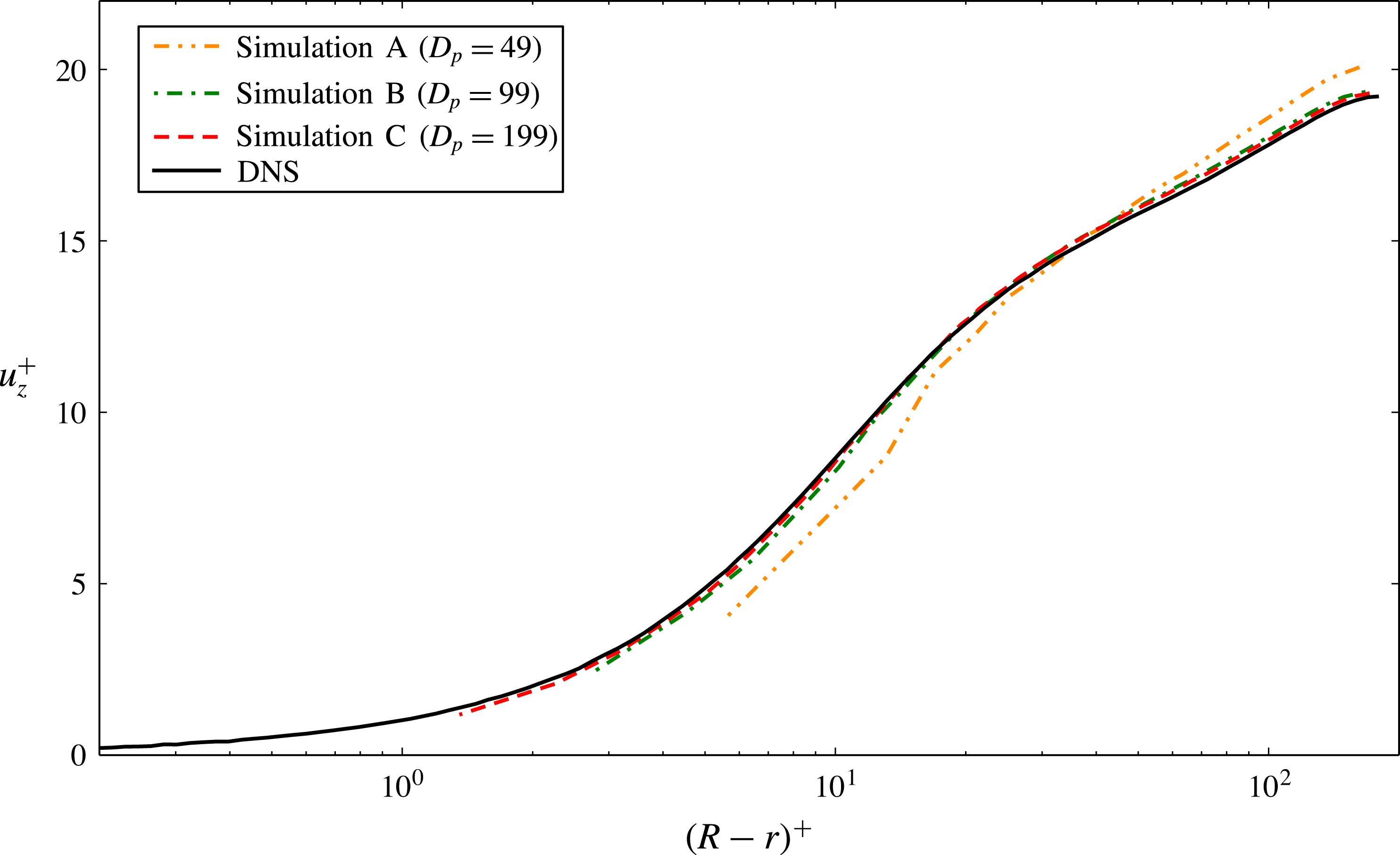
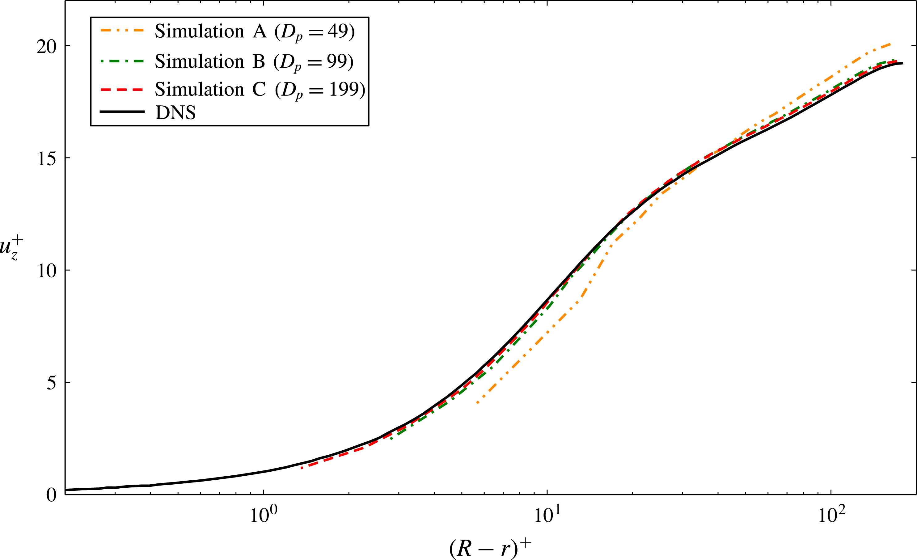
Figure 3 shows a comparison of the mean stream-wise velocity component of runs A–C to the reference DNS results. Despite severe under-resolution, excellent agreement can be observed for runs B and C. Run A obviously employs a mesh which is too coarse to capture the scaling of the mean velocity correctly.
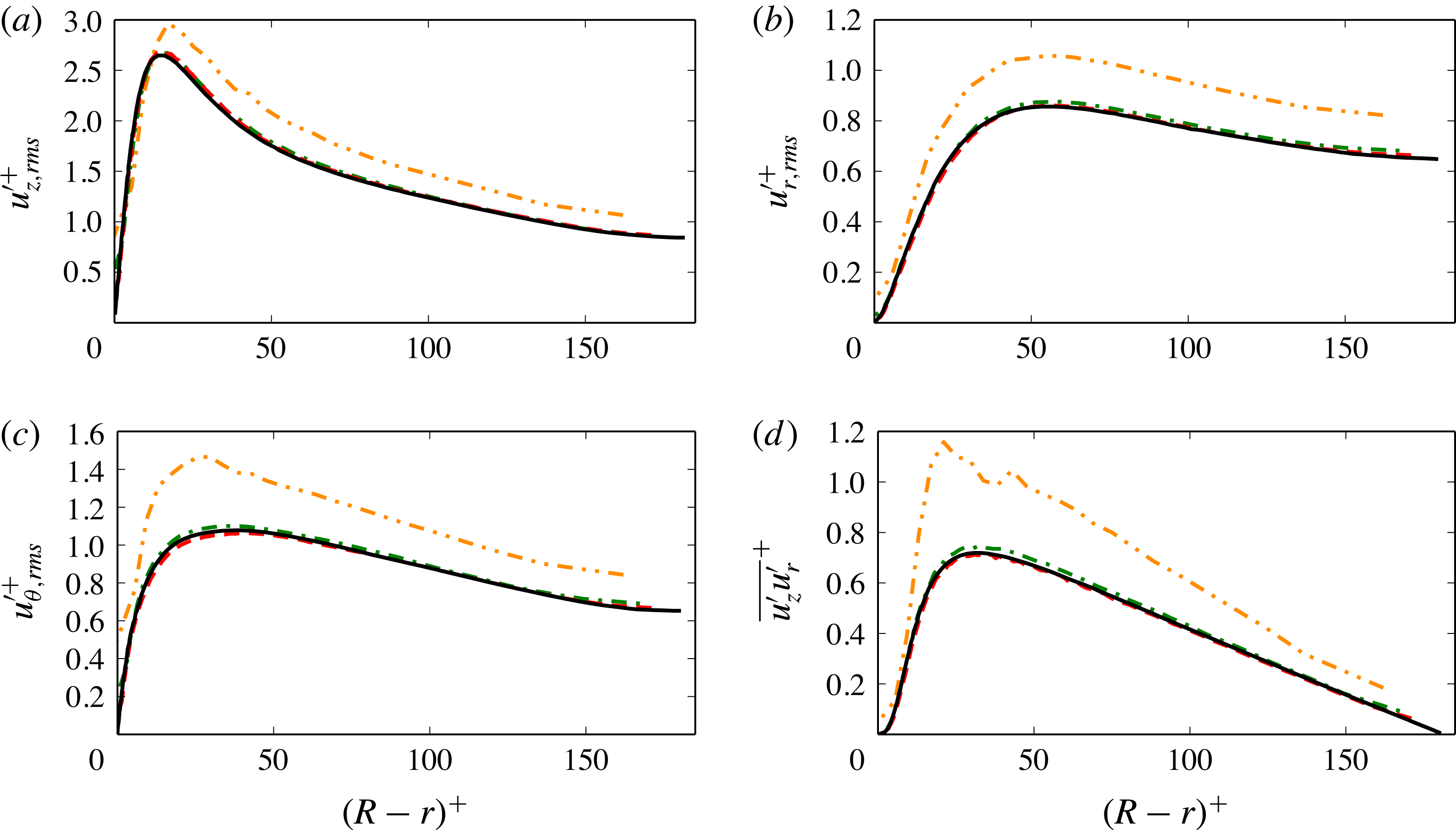
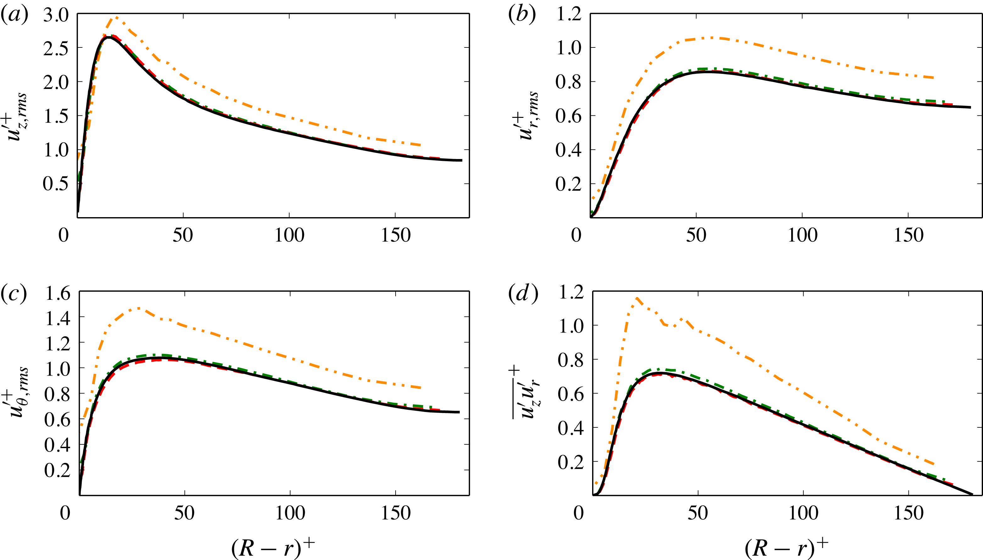
The next order statistical moments are shown in figure 4(a–d). The root-mean-square (r.m.s.) fluctuations of the axial, radial and azimuthal velocity component show the same trend as seen in figure 3; the coarsest simulation does not reproduce the expected values while runs B and C are very close to the DNS results. Moreover, the cross-correlations of the axial and radial fluctuations, figure 4(d), show excellent agreement for simulations B and C as well.
Mean velocity component in flow direction for the turbulent pipe flow.
Root mean square velocity profiles for the turbulent pipe flow. The legend is identical to figure 3.
3.3 Sedimenting sphere
The flow in the valve/piston assembly is induced through the moving piston and it is expected that the treatment of the moving boundary has a significant influence on the flow field inside the chamber. Stability and accuracy of the wall-boundary treatment as outlined in § 2.1 were investigated for various flow set-ups including moving objects in two dimensions in Dorschner et al. (Reference Dorschner, Chikatamarla, Bösch and Karlin2015). Here, we present a three-dimensional validation, where a sedimenting rigid sphere is considered. The sphere with density
 ${\it\rho}_{s}$
is resolved with a diameter of
 $D_{s}=30$
and the particle Reynolds number was taken to be
 $Re=100$
. When released from rest in a quiescent fluid with density
 ${\it\rho}_{f}$
, the sphere accelerates to its asymptotic settling velocity
 $u_{t}$
, where the gravitational force
 $F_{g}={\rm\pi}D_{s}^{3}{\it\rho}_{s}g/6$
is balanced by the buoyancy force
 $F_{b}={\rm\pi}D_{s}^{3}{\it\rho}_{f}g/6$
and the drag force
 $F_{d}=({\it\rho}_{f}u^{2}{\rm\pi}D_{s}^{2}C_{d})/8$
. The force balance immediately yields
 $$\begin{eqnarray}\displaystyle \frac{{\it\rho}_{s}}{{\it\rho}_{f}}=1+\frac{3u_{t}^{2}C_{d}}{4D_{s}g}, & & \displaystyle\end{eqnarray}$$
where
 $C_{d}$
denotes the drag coefficient. We set the nominal settling velocity to
 $u_{t,n}=0.01$
in lattice units and choose the particle density in accordance with (3.10). The drag coefficient was measured in a separate simulation for a stationary sphere and a mean flow velocity, which resulted in
 $C_{d}=1.1$
in agreement with literature values (see, e.g., Roos & Willmarth Reference Roos and Willmarth1971; Johnson & Patel Reference Johnson and Patel1999; Kim, Kim & Choi Reference Kim, Kim and Choi2001). In the dynamic case, we solve Newton’s equations for the particle motion
 $$\begin{eqnarray}\displaystyle & \displaystyle \frac{\text{d}\boldsymbol{x}_{s}}{\text{d}t}=\boldsymbol{u}_{s}, & \displaystyle\end{eqnarray}$$
 $$\begin{eqnarray}\displaystyle & \displaystyle \frac{\text{d}\boldsymbol{u}_{s}}{\text{d}t}=\frac{\boldsymbol{F}}{m_{s}}+\left(1-\frac{{\it\rho}_{f}}{{\it\rho}_{s}}\right)\boldsymbol{g}, & \displaystyle\end{eqnarray}$$
where the force
 $\boldsymbol{F}$
acting on the particle was evaluated using the momentum exchange method (see, e.g., Mei et al.
Reference Mei, Yu, Shyy and Luo2002). We measure the terminal settling velocity to be
 $u_{t}=0.0100033$
, which amounts to less than
 $0.033\,\%$
error. Its equivalence to the nominal settling velocity establishes Galilean invariance between the static and the dynamic case and therefore validates the moving boundary condition.
4 Valve/piston assembly
With the results of the preliminary studies in the previous section, we now consider the flow in a valve/piston assembly. To that end, we shall compare it to the recent DNS simulations of Schmitt et al. (Reference Schmitt, Frouzakis, Tomboulides, Wright and Boulouchos2014a ) and the experimental data of Morse et al. (Reference Morse, Whitelaw and Yianneskis1979) for different resolutions.
These simulations when viewed together with other existing benchmark simulations performed for flow between parallel plates and flow past a circular cylinder (Chikatamarla & Karlin Reference Chikatamarla and Karlin2013) establish the reliability of entropic LB models for turbulent flows. Moreover, in the context of subgrid simulations, a simple grid convergence study (similar to DNS simulations) is sufficient to establish the viability and accuracy of the simulations. This feature, combined with a second-order convergence to DNS solution in almost all simulations and the lack of any tuning parameters in the model, gives us the confidence to explore further complex flow set-ups such as valve/piston assembly.
4.1 Numerical set-up
The numerical set-up is identical to the experimental work of Morse et al. (Reference Morse, Whitelaw and Yianneskis1979) and the DNS of Schmitt et al. (Reference Schmitt, Frouzakis, Tomboulides, Wright and Boulouchos2014a
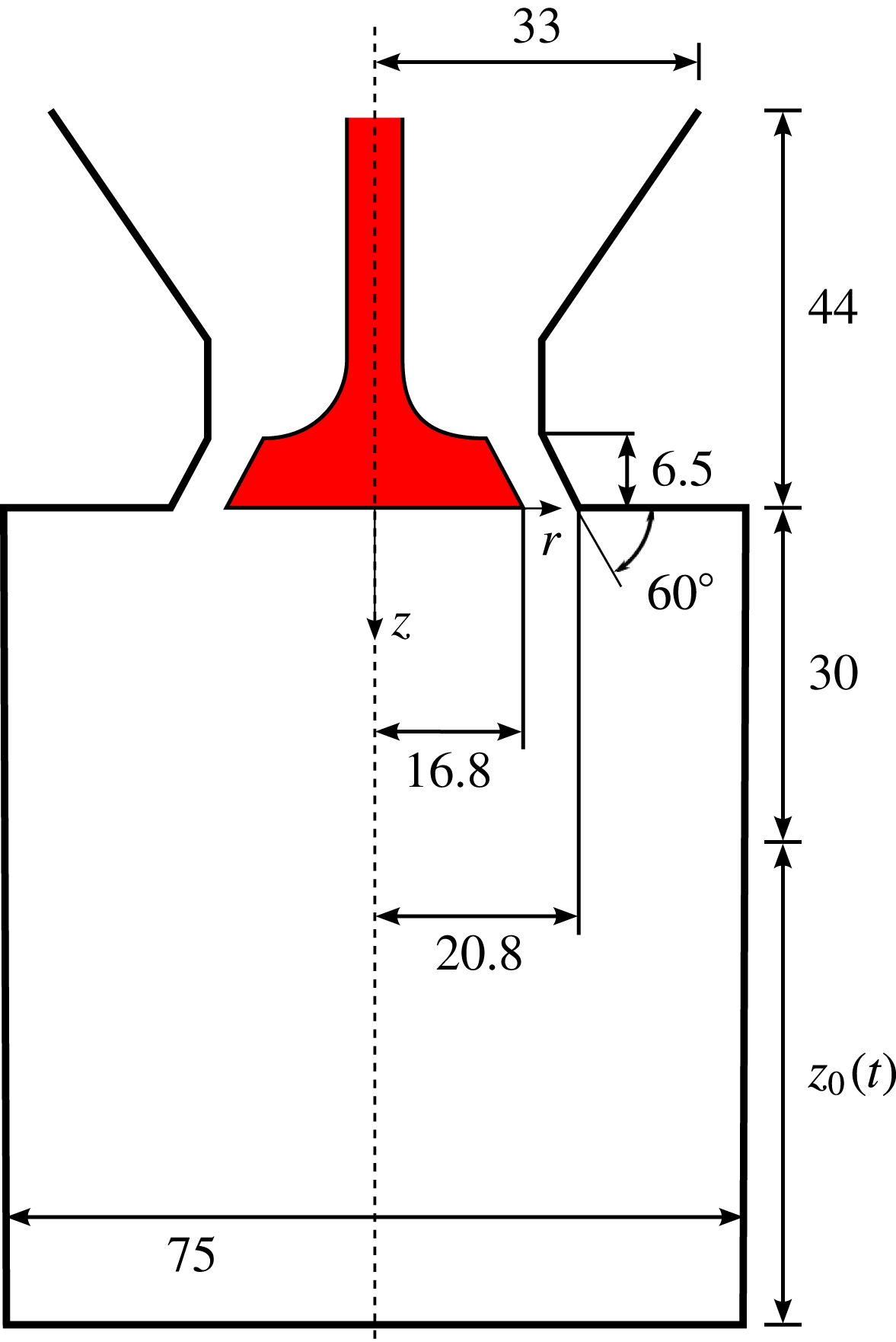
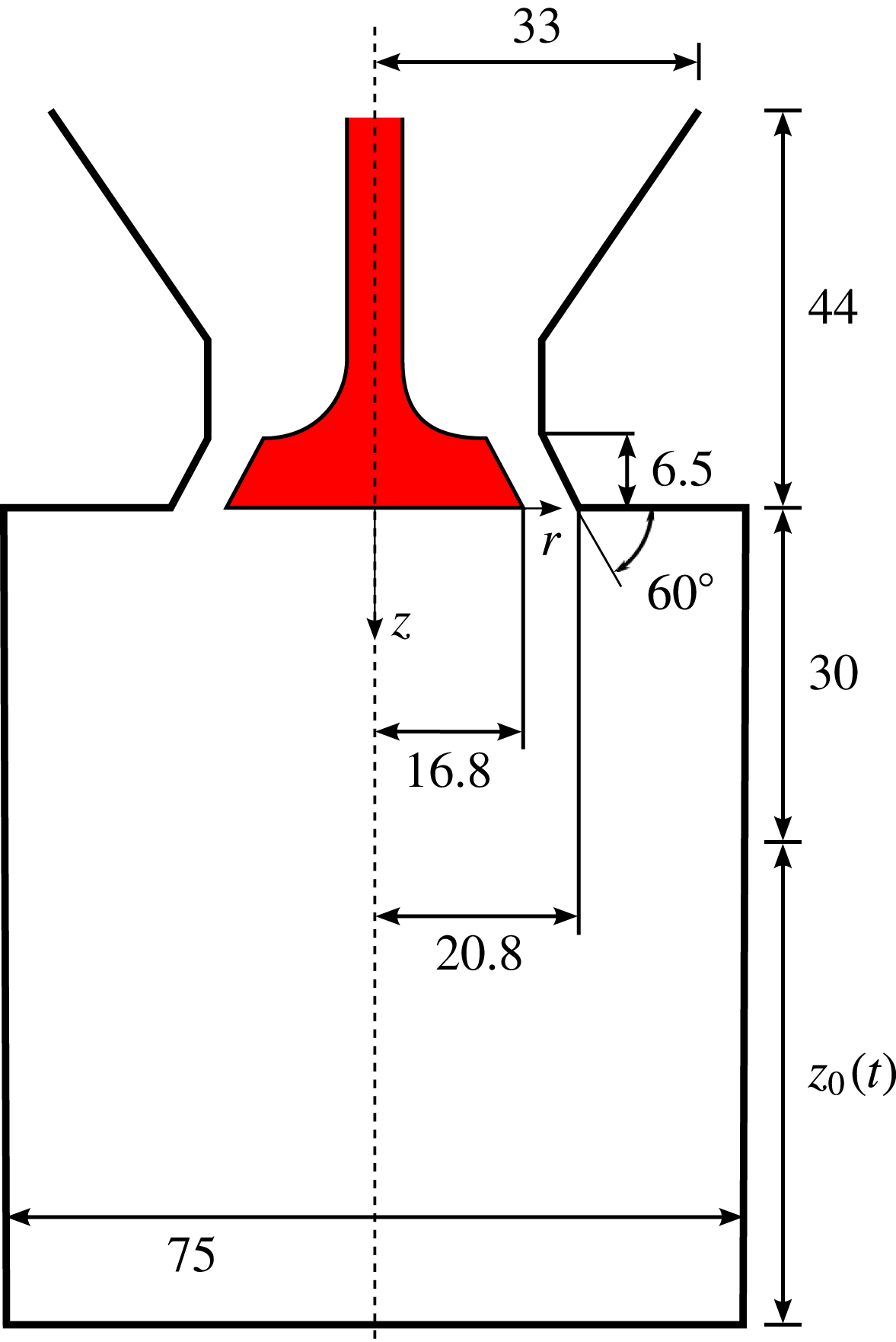
) for which the schematic and all geometrical specifications are shown in figure 5. The axis-symmetric assembly consists of a cylinder with diameter
 $D_{c}=75$
mm, a static centred valve and a flat piston for which a sinusoidal motion corresponding to a speed of
 $200$
rpm, a stroke of
 $S=60$
mm and a clearance at top dead centre (TDC) of
 $30$
mm is imposed. The maximum piston speed and the viscosity were chosen to obtain a Reynolds number of
 $Re=v_{p,max}D_{c}/{\it\nu}=3070$
. The valve has the radius
 $r_{v}=16.8$
mm and an angle of
 $30^{\circ }$
, which results in a uniform valve gap of approximately
 $4$
mm. In the experiment, the system is open and was mimicked in our simulation by a large reservoir on top of this assembly (not shown in the schematic) with a volume roughly three times as large as displaced by the cylinder. Due to the open system, compressibility effects are negligible and the flow may be regarded as incompressible without any phase change. Initially, a quiescent flow field is imposed where the piston is located at TDC. Further, the inlet condition at the top of the reservoir is evaluated instantaneously using the current piston velocity and the ratio of the reservoir and piston area. For all other boundary conditions, the no-slip boundary condition as outlined in § 2.1 is imposed.
Schematic of the valve/piston assembly (all measures are given in mm).
In total, eight cycles were simulated (see the supplementary movie available athttp://dx.doi.org/10.1017/jfm.2016.448) and the first two were neglected in the accumulation of statistics to avoid initialization effects. Statistical quantities were computed using azimuthal and ensemble (across cycles) averaging. To study the nature of the subgrid model, simulations were carried out for a cylinder resolution of
 $D_{c,lb}=\{100,150,300\}$
points, respectively. This yields a total of approximately
 $N=\{8.5,28,228\}\text{Mio}$
nodes for each simulation and a cubic domain, respectively. The resolutions were chosen based on our preliminary studies in § 3 for which the flow regimes in terms of Reynolds number are similar to the one exhibited here.
Using a CRAY XC40 system the computational resources for
 $D_{c,lb}=300$
amount to
 $8.6\times 10^{3}\text{CPUh}$
per cycle, which is roughly
 $20$
times less than the corresponding requirement for the DNS in Schmitt et al. (Reference Schmitt, Frouzakis, Tomboulides, Wright and Boulouchos2014a
). The computational cost scales as
 $p^{D+1}$
for a refinement ratio
 $p$
and the dimensionality
 $D$
. Note that since a cubic domain and a regular grid without any local mesh refinement is used, significant optimization options remain. This is focus of future work as the scope of the study herein is to validate the implicit subgrid model of KBC for complex flows beyond classical benchmarks.
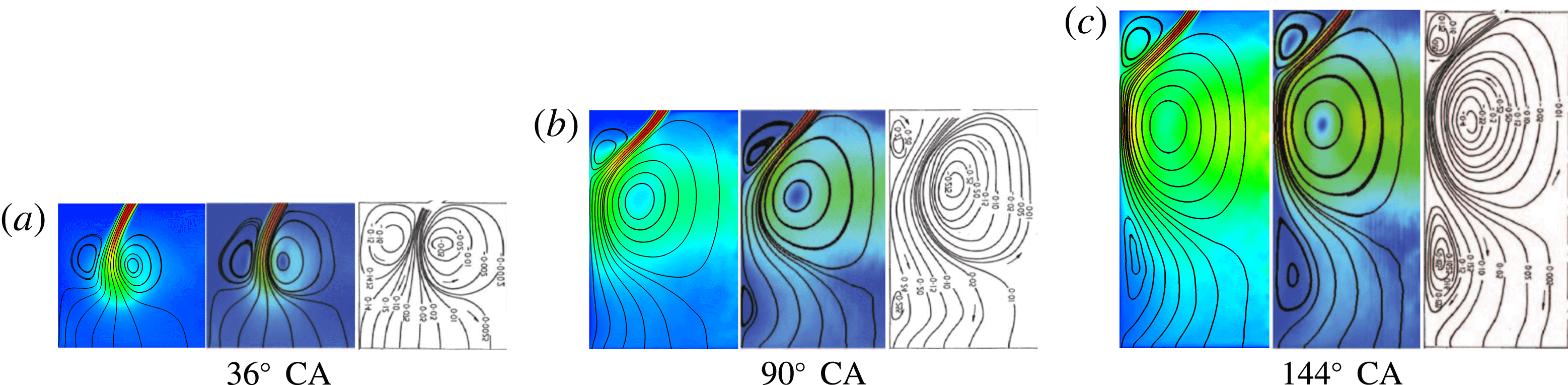
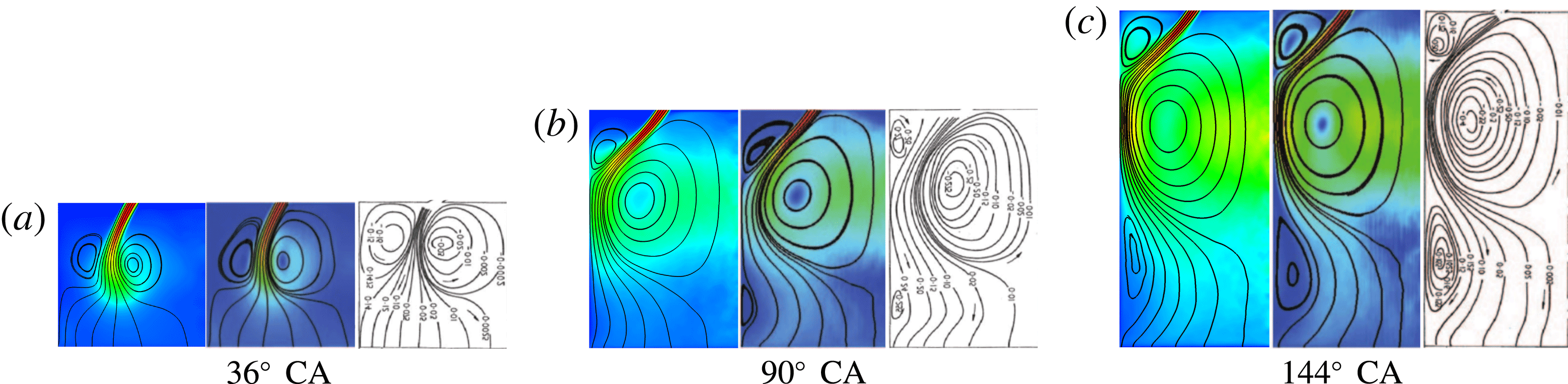
Comparison of streamlines of the averaged velocity field. From (a) to (c): present results, DNS and experimental data are shown for different crank angles, respectively.
4.2 Velocity field
Resolved simulation and the DNS limit
In this section, we report the radial velocity profiles obtained for the intake stroke at crank angles (CA) of
 $36^{\circ }$
,
 $90^{\circ }$
and
 $144^{\circ }$
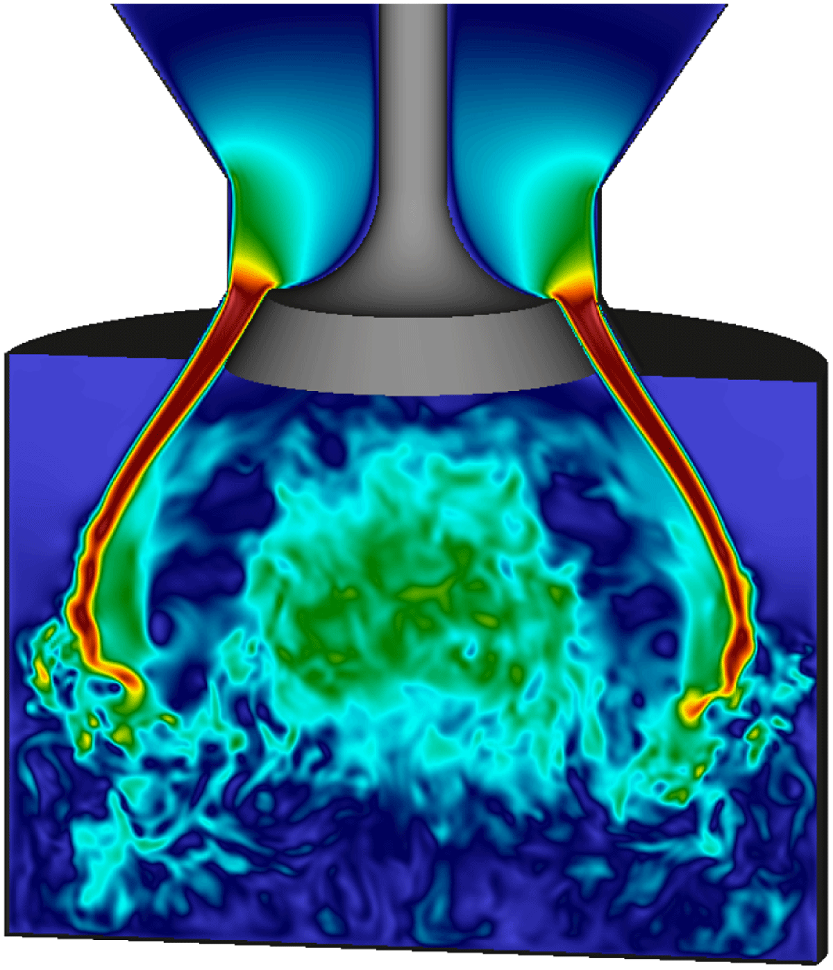
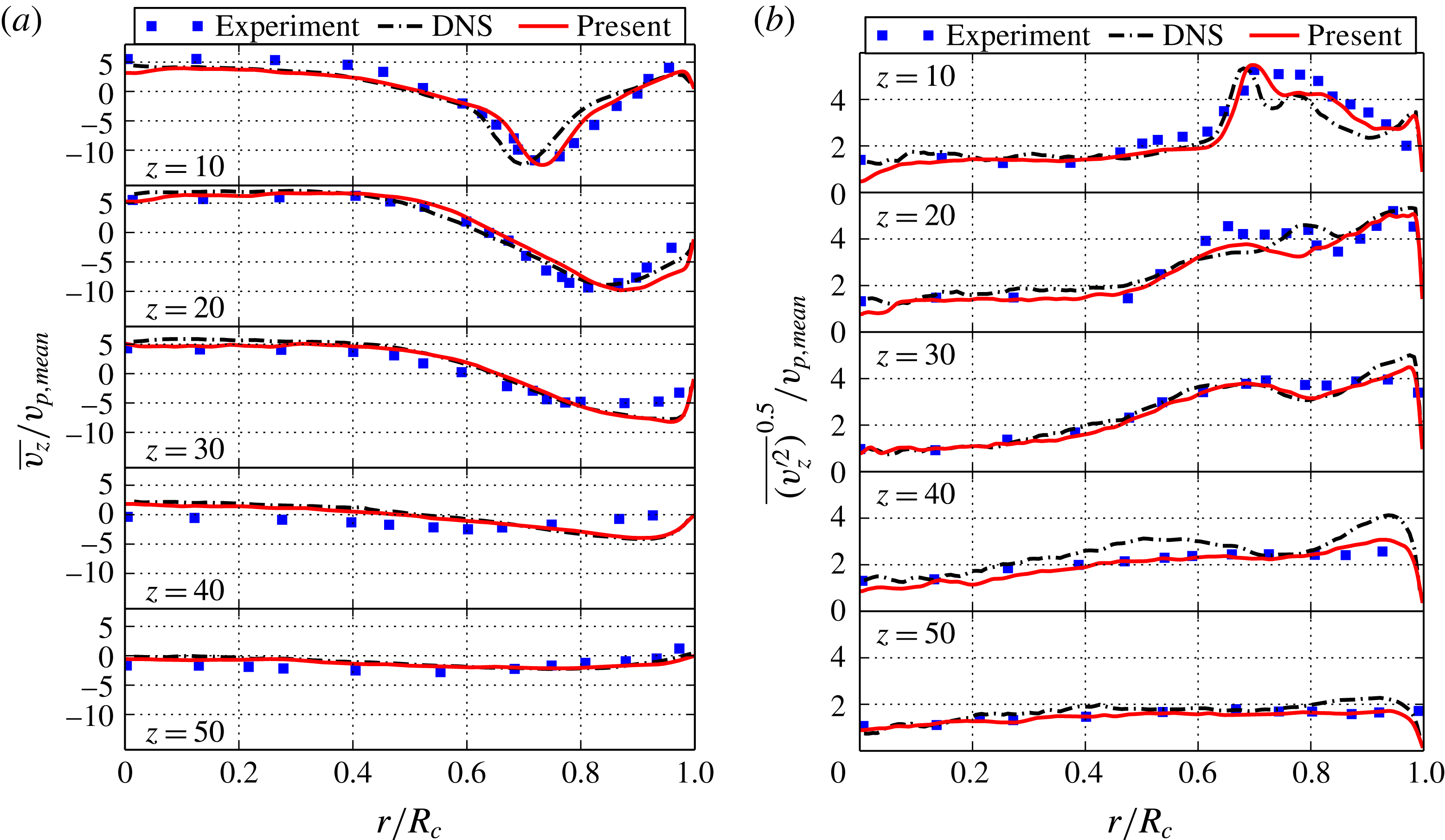
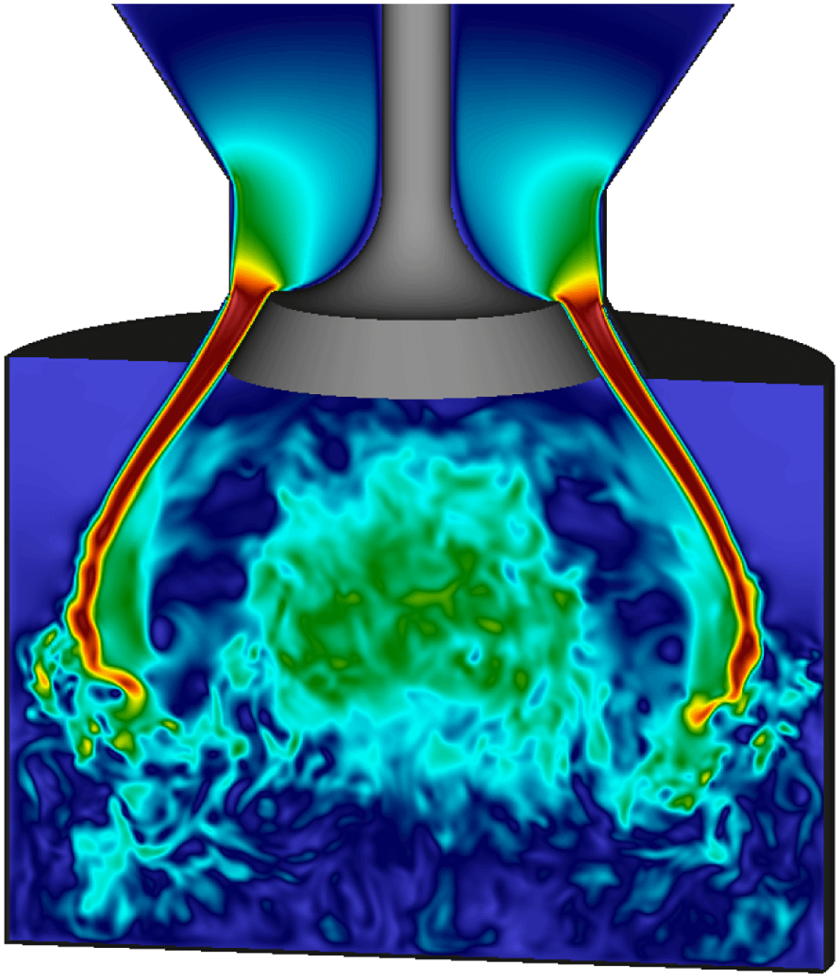
on different axial planes and make a comparison with the DNS and the experimental data. In the first instance, the profiles for the highest resolution are compared to establish the correct convergence of KBC models. Later in this section, the influence of under-resolution and its convergence is investigated. The main features of the mean flow field may be identified by the averaged streamlines shown in figure 6. In good agreement with both experimental and DNS data, the first phase of the intake stroke consists of fluid drawn into the chamber by the accelerated motion of the piston, forming a hollow cone jet. As a consequence, small vortex rings on both sides of the jet are generated, where the inner ring develops into the main feature as the piston moves further down and deflects the jet inwards before it is reflected by the piston. At this stage, one may observe jet breakup processes and the transition to turbulence caused by the interaction with the flow field. For instance, the Kelvin–Helmholtz instabilities in the shear layer are captured in the velocity snapshot of figure 7 for the first cycle. Subsequently, the jet is deflected towards the cylinder wall and a third vortex becomes apparent in the averaged flow field (see figure 6
c).
Note that at
 $90^{\circ }$
CA the flow undergoes a transition phase as the jet has reached its highest momentum and a fully turbulent flow field, dominated by the large vortical structure, is developed by interaction of the jet with the flow field.
Instantaneous velocity magnitude snapshot at
 $77^{\circ }$
CA.
Quantitatively we compare the corresponding mean and r.m.s. velocity profiles of the axial velocity component
 $v_{z}$
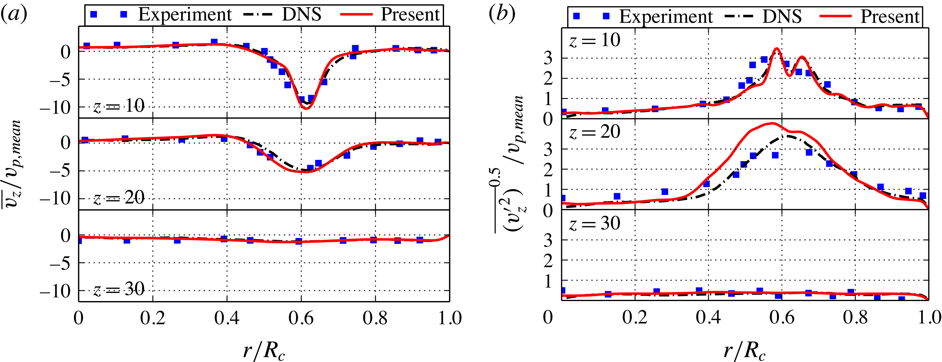
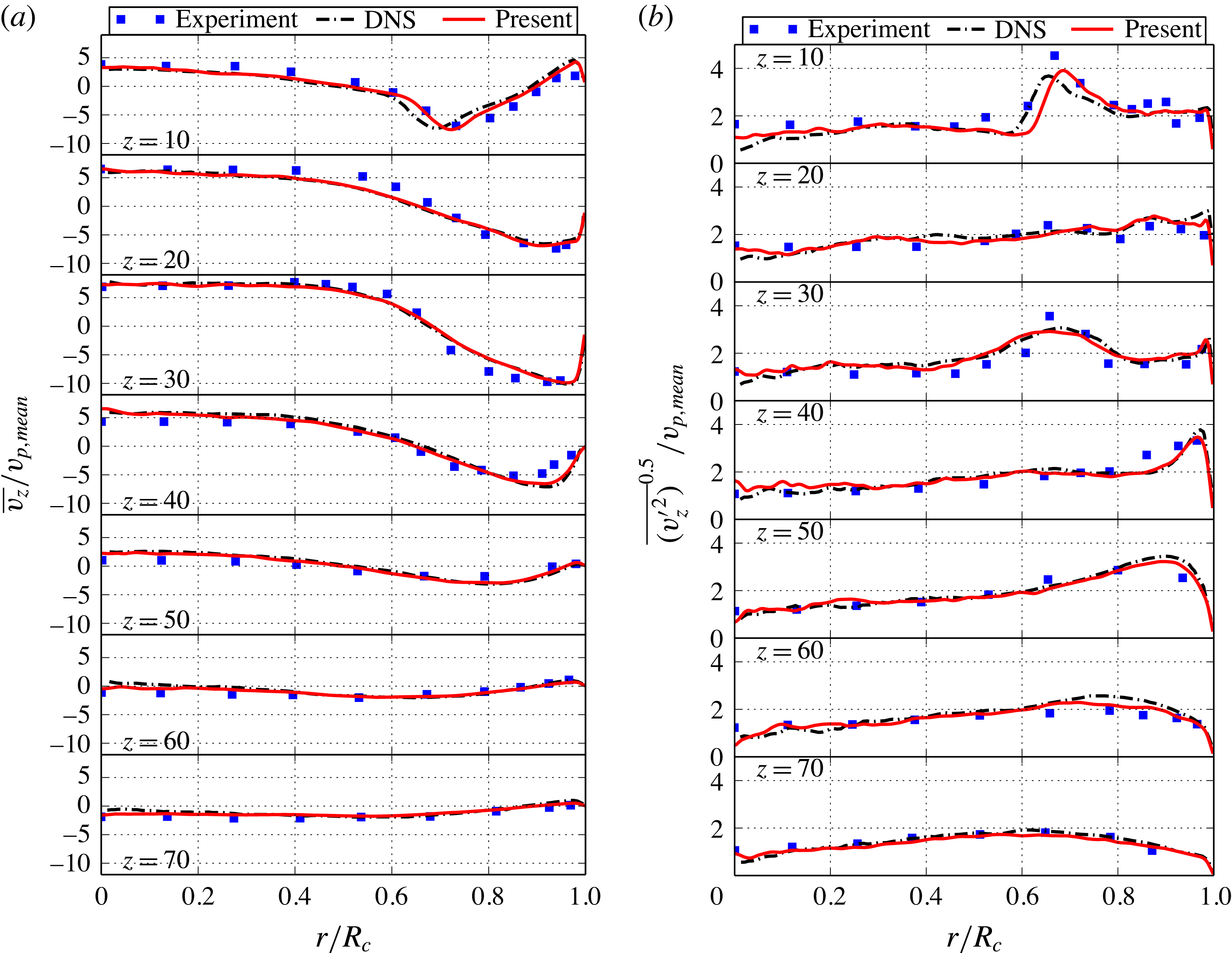
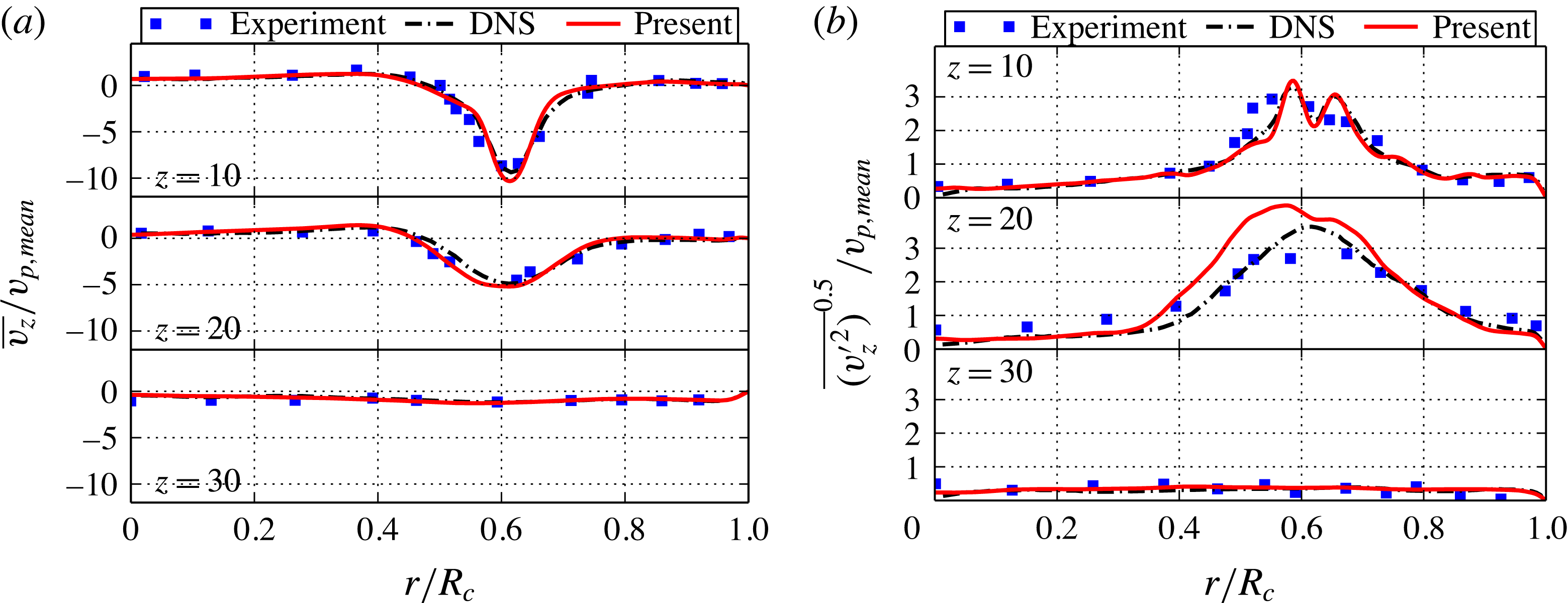
in radial direction on different axial planes with respect to the cylinder head in figures 8–10). Consistent with the previous observation, the flow at
 $36^{\circ }$
CA is mainly dominated by the incoming jet, which results in a peak velocity at
 $r/R_{c}\approx 0.6$
. The r.m.s. velocity profiles indicate that the turbulence generation may be localized to jet shear layer on both sides. It is clear that the results predicted by the presented KBC model compare well to both DNS and experiment in terms of mean jet velocities and location. The r.m.s. velocities near the cylinder head at
 $z=10$
mm are also on top of the DNS data. It is apparent that more turbulence is generated compared to DNS and experiment close to the cylinder axis for the
 $z=20$
mm plane, resulting in a broadening of the r.m.s. velocity profile towards the centre. However, this does not seem to affect the good agreement for different crank angles as shown below.
At
 $90^{\circ }$
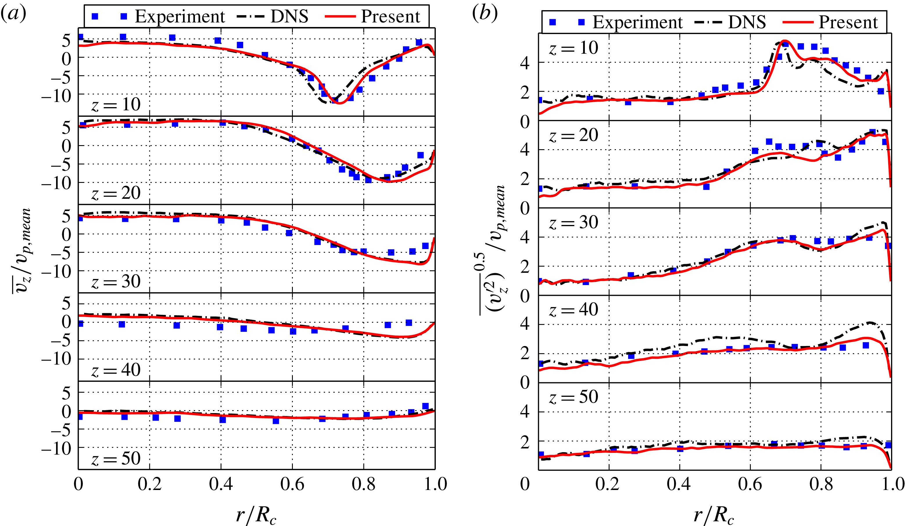
CA, the deflection of the jet at the cylinder wall leads to an increase of the jet radius, which is manifested by a shift of the average velocity profiles towards the cylinder wall. It should be noted that, as observed in the LES study of Liu & Haworth (Reference Liu and Haworth2010), the flow transition at this stage of highest momentum is difficult to capture for various turbulence modelling approaches. In their work, better agreement was achieved by adapting the model parameters but led to more discrepancies for
 $36^{\circ }$
CA and
 $144^{\circ }$
CA. Despite that, figure 9 clearly shows excellent agreement with the KBC model for both mean and r.m.s. velocity profiles compared with the reference data. A small shift in radial direction compared to the DNS is visible for the upper axial planes and the mean profiles but matches the experimental data. In planes beyond
 $z=20$
mm, our simulation is almost indistinguishable from the DNS result. Analogously, this holds for the r.m.s. velocity profiles.
Comparison of the ensemble and azimuthally averaged axial mean (a) and r.m.s. (b) velocities at
 $36^{\circ }$
CA for a resolution of
 $D_{c,lb}=300$
.
Comparison of the ensemble and azimuthally averaged axial mean (a) and r.m.s. (b) velocities at
 $90^{\circ }$
CA for a resolution of
 $D_{c,lb}=300$
.
Comparison of the ensemble and azimuthally averaged axial mean (a) and r.m.s. (b) velocities at
 $144^{\circ }$
CA for a resolution of
 $D_{c,lb}=300$
.

At later crank angles, the piston is decelerating and we compare the corresponding profiles for
 $144^{\circ }$
CA in figure 10. Similarly, the discrepancies are marginal for all data.
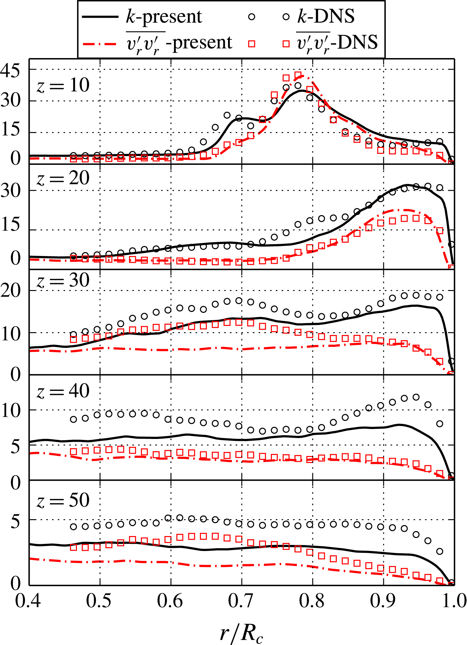
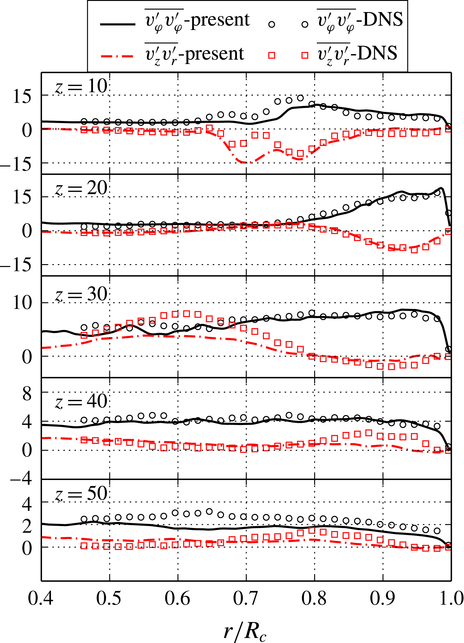
Next, let us consider the turbulence statistics of the flow field by means of the Reynolds stress components and the turbulent kinetic energy
 $k$
as shown in figures 11–12. As the comparison is very similar during all phases, we choose the most interesting transition phase at
 $90^{\circ }$
CA as representative. It can clearly be seen that the turbulent kinetic energy follows the trend of the reference data. Its shift is analogous to the mean and r.m.s. velocities as shown above and minor discrepancies in terms of magnitude are visible. This, however, becomes more pronounced for lower values of the kinetic energy, suggesting that the contribution of the smallest scales is not fully accounted for. Similarly, the radial component
 $\overline{v_{r}^{\prime }v_{r}^{\prime }}$
shows a good agreement for the region near the jet entry, but dissipates slightly more. Analogous behaviour may be found for the Reynolds stress component
 $\overline{v_{{\it\varphi}}^{\prime }v_{{\it\varphi}}^{\prime }}$
and
 $\overline{v_{z}^{\prime }v_{r}^{\prime }}$
.
Under-resolved simulations
The above comparison demonstrated an overall excellent agreement between DNS, experimental data and our simulation using the entropic multi-relaxation time lattice Boltzmann model and the highest resolution of
 $D_{c,lb}=300$
. This provides evidence for the convergence of our simulations to DNS. Having established the correct limit, we can now study the effect of under-resolution.
Comparison of the ensemble and azimuthally averaged turbulent kinetic energy
 $k$
and the Reynolds stress component
 $\overline{v_{r}^{\prime }v_{r}^{\prime }}$
at
 $90^{\circ }$
CA for a resolution of
 $D_{c,lb}=300$
.

Comparison of the ensemble and azimuthally averaged Reynolds stress components
 $\overline{v_{{\it\varphi}}^{\prime }v_{{\it\varphi}}^{\prime }}$
and
 $\overline{v_{z}^{\prime }v_{r}^{\prime }}$
at
 $90^{\circ }$
CA for a resolution of
 $D_{c,lb}=300$
.

The discussion is similar for all crank angles and we again choose the most critical phase at
 $90^{\circ }$
CA as representative. In figure 13, the mean and r.m.s. velocity profiles are shown for cylinder resolutions of
 $D_{c,lb}=\{100,150,300\}$
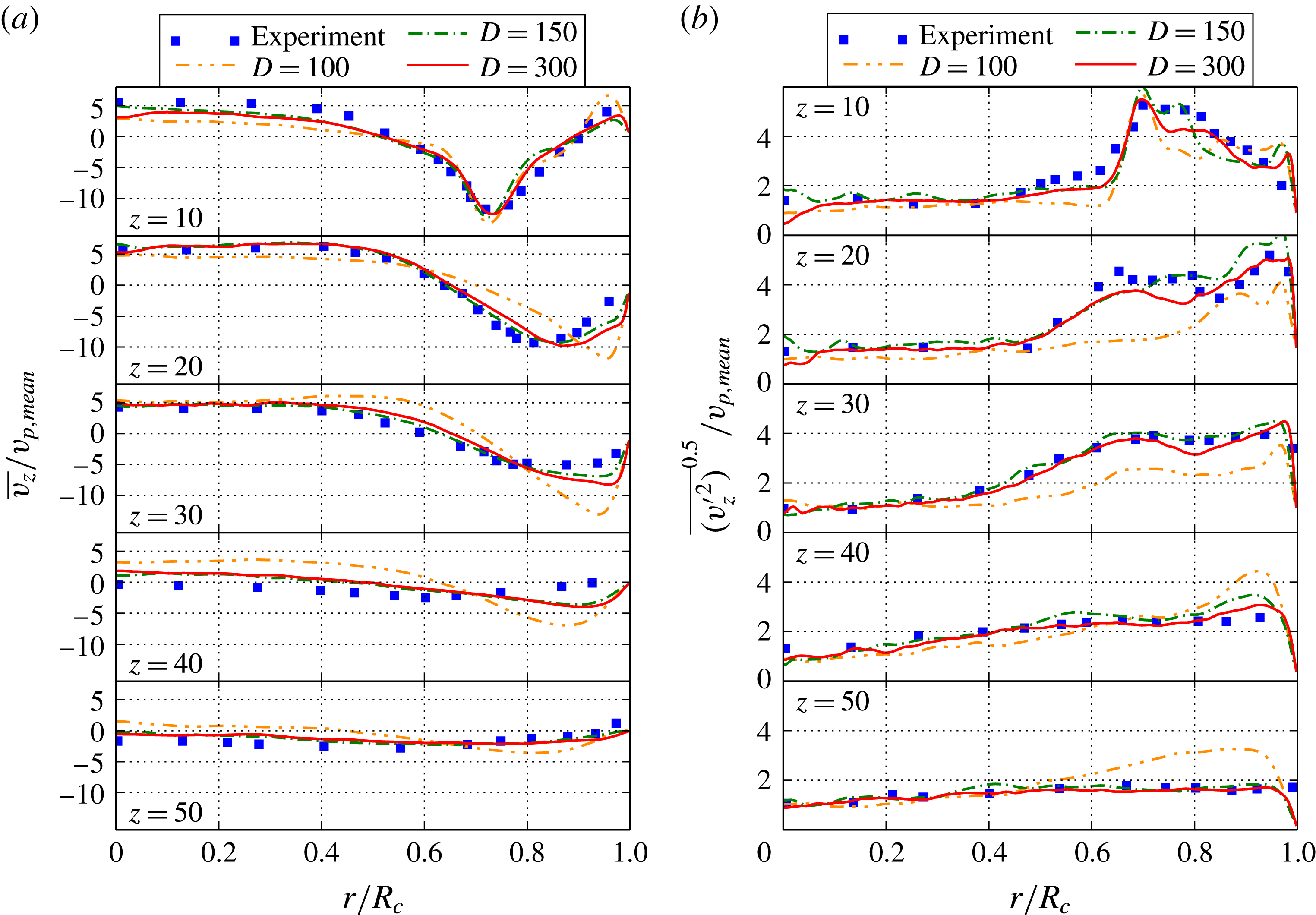
points. It may be observed that the differences in terms of the average axial velocity profiles between
 $D_{c,lb}=150$
and
 $D_{c,lb}=300$
are marginal. The r.m.s. velocity profiles are very similar as well and only a small over-prediction at the lower resolution may be observed. At first sight, this is not intuitive as one would expect the turbulence production to be smoothed out, which would lead to lower values of the r.m.s. velocities. However, in this case, it may be traced back to very subtle inaccuracies of jet breakup processes, which affect the formation of the large-scale structures of the flow in a nonlinear manner and in turn affect the turbulence production leading to slightly higher r.m.s. values. On the other hand, for the case of
 $D_{c,lb}=100$
, the effect of under-resolution becomes noticeable. The incoming jet is hardly broken up by the surrounding flow field but rather by the confining cylinder walls, which leads to a higher penetration depth and jet radius on average. This may also be seen when considering the corresponding r.m.s. profiles, where the consistent under-prediction for
 $z=10{-}30$
mm leads to less turbulence production and therefore a delayed jet breakup with an increased diameter. Note that this is well within expectations as the valve gap is resolved by only three fluid points for this case. A comparison to our previous simulations of the pipe would suggest that the resolution is sufficient even at
 $D_{c,lb}=100$
. However, it needs to be kept in mind that due to the impinging jet the Kàrmàn number varies in the range of
 $R^{+}=u_{{\it\tau}}R/{\it\nu}\approx 90{-}780$
(measured for
 $D_{c,lb}=300$
) and that for the local maximum of
 $R^{+}\approx 780$
the effect of the small-scale structures cannot be captured accurately at this resolution. On the other hand, the Kida vortex simulation reveals that the small structures in the bulk of the chamber are not correctly represented for a resolution as coarse as
 $D_{c,lb}=100$
, which further suggests that their contribution to the jet breakup is not fully accounted for. Hence, as expected, the complex flow in the cylinder as a combination of distinct flow features requires a higher resolution than the individual building blocks. A slight increase in resolution to
 $D_{c,lb}=150$
is necessary. Note that as indicated by the precursor simulations in §§ 3.1 and 3.2, this is still an under-resolved simulation in which the built-in subgrid model of KBC captures almost all flow features accurately.
Comparison of the ensemble and azimuthally averaged axial mean (a) and r.m.s. (b) velocities at
 $90^{\circ }$
CA for different resolutions.

4.3 Cyclic variability
Capturing cyclic variability in internal combustion engine simulations is of crucial importance for its design as it may significantly influence its efficiency and pollutant formation among various other effects. Such variability has also been observed both numerically and experimentally in the valve/piston assembly (Haworth Reference Haworth1999; Rutland Reference Rutland2011; Schmitt et al. Reference Schmitt, Frouzakis, Tomboulides, Wright and Boulouchos2014a ). Its origin was discussed in the DNS work of Schmitt et al. (Reference Schmitt, Frouzakis, Wright, Tomboulides and Boulouchos2014b ), where it was mainly attributed to the remaining radial velocity at TDC from the previous cycle, the consequential jet location as well as the vortex ring orientation at bottom dead centre (BDC).
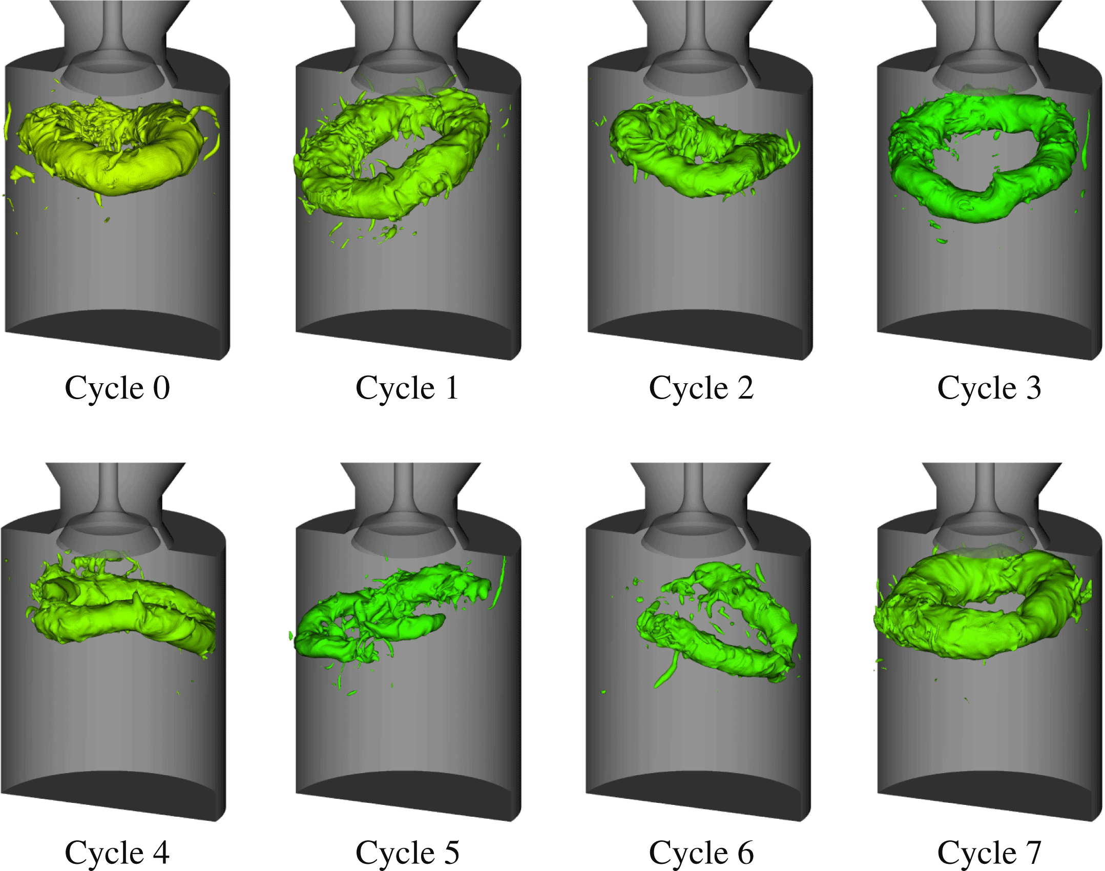
The aim of this section is to investigate the predictive capabilities of KBC models concerning the cyclic variability. An indicator of cyclic variability is given by the large vortex ring formed at BDC, which is visualized for all simulated cycles in figure 14 by means of the pressure iso-surfaces. Variation in shape, size and orientation is observed. Particularly pronounced is the distortion of the vortex ring for cycles five and six.
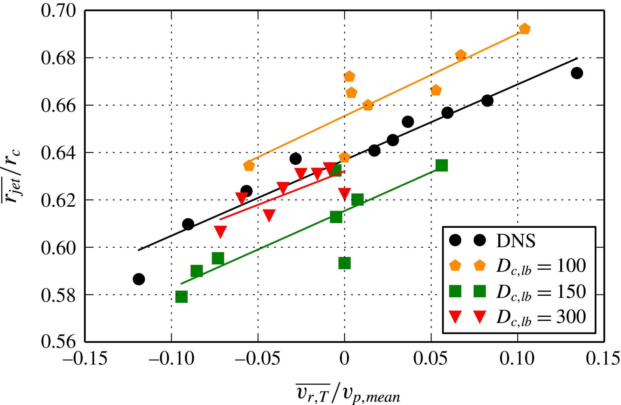
Quantitatively, we compare the correlation plot of the normalized, average radial velocity
 $\overline{v_{r,T}}/v_{p,mean}$
at TDC versus the normalized, average jet radius
 $\overline{r_{jet}}/r_{c}$
at
 $45^{\circ }$
CA in figure 15. Both quantities are evaluated as in Schmitt et al. (Reference Schmitt, Frouzakis, Wright, Tomboulides and Boulouchos2014b
), where the radial velocity is averaged at TDC azimuthally and radially in an axial window of
 $11.5$
mm starting from the cylinder head. The mean jet radius is defined as the average of the jet radii contained in the iso-surface of
 $u_{z}=-2.5~\text{m s}^{-1}$
. Our results show that the phenomenon of a cyclic varying jet radius is observed for all resolutions and confirm the result of Schmitt et al. (Reference Schmitt, Frouzakis, Wright, Tomboulides and Boulouchos2014b
) that it may be correlated to the residual turbulence at TDC from the previous cycle, where an increased averaged radial velocity at TDC results in an increased average jet radius and vice versa. It is notable that even the lowest resolution, for which the average axial velocity profiles have shown effects of under-resolution, exhibits pronounced cycle-to-cycle variation with the qualitatively correct cause and effect relation. This is indicated in figure 15, where the linear curve fit has an almost identical slope for all resolutions and therefore establishes the correlation of the normalized, average radial velocity
 $\overline{v_{r,T}}/v_{p,mean}$
at TDC versus the normalized, average jet radius
 $\overline{r_{jet}}/r_{c}$
. In addition, figure 15 reflects the dominant contributions to the subsequent jet breakup and is consistent with our previous observations in figure 13. For the lowest resolution, one can observe the most severe increase of the mean jet radius, which again may be attributed to the fact that the incoming jet is less influenced by the unresolved small-scale flow structures but rather is broken up by the interaction with the chamber walls leading to a broader jet with higher penetration depth. This was also observed for mean velocity profiles in figure 13. As the resolution is increased, the contributions of the small-scale structures become more pronounced and their interaction with the jet do not allow for such large jet radii as in the under-resolved case. On average this yields a lower penetration depth and smaller jet radii, consistent with both DNS and experimental data. As expected, the highest resolution yields the best match in terms of the average jet radius. More simulated cycles will presumably increase the spread on both the jet radius variability as well as the mean radial velocity.
Cyclic variation of the vortex ring at BDC visualized by pressure iso-surfaces for
 $D_{c,lb}=300$
.

Cyclic variation for all resolutions of
 $D_{c,lb}=\{100,150,300\}$
and the DNS results, quantified by mean jet radius
 $\overline{r_{jet}}/r_{c}$
at
 $45^{\circ }$
CA and correlated to the mean radial velocity
 $\overline{v_{r,T}}/v_{p,mean}$
at TDC. Lines represent a linear fit through the corresponding data points.

5 Concluding remarks
In this work, we have presented a detailed study of a novel entropic multi-relaxation time lattice Boltzmann model for simple and complex flows for both resolved and under-resolved simulations. It was shown that the KBC model converges towards DNS simulations and experimental results in terms of average velocities, Reynolds stress components and the turbulent kinetic energy for both simple and complex flow set-ups. For under-resolved cases, the entropy-based, implicit subgrid model shows predictive capabilities already at grids eight times smaller than the resolved case. With further coarsening, the effect of under-resolution becomes noticeable but is expected as only three fluid nodes are used in the valve opening. This can be improved with appropriate grid-refinement in the region of interest and is left for future work. More importantly, this study shows that kinetic methods with built-in subgrid capabilities become reliable without the need for identifying and refining the grid in regions of high spacial gradients (such as near wall regions and jet breakup regions). Also, excellent results were obtained on a static grid as compared to a moving grid which are commonly used for such valve/piston set-ups, thus significantly reducing the complexity of the algorithm and realization. The problem of using appropriate grids for each particular flow set-up is commonplace for simulation of fluid flows and requires knowledge and expertise on the flow set-up at hand. This process is heavily simplified due to the built-in subgrid nature of the entropic lattice Boltzmann models which allow the use of simple Cartesian meshes for such complex flow set-ups and still retain predictive capabilities. Thus, the KBC model may be considered as a robust, parameter-free, efficient and accurate alternative to state-of-the-art modelling techniques such as LES. Apart from simplicity in the choice of grid and implementation, these kinetic methods can significantly reduce the computational costs, especially for complex flow set-ups with moving walls.
Acknowledgements
This work was supported by the European Research Council (ERC) advanced grant no. 291094-ELBM and the ETH-32-14-2 grant. The computational resources at the Swiss National Super Computing Center (CSCS) were provided under grants s492 and s630.
Supplementary movie
A supplementary movie is available at http://dx.doi.org/10.1017/jfm.2016.448.
Appendix A. Moment representation of the populations
For ease of notation, let us introduce the trace of the stress tensor
 $$\begin{eqnarray}\displaystyle \unicode[STIX]{x1D61B}=M_{200}+M_{020}+M_{002}, & & \displaystyle\end{eqnarray}$$
the normal stress differences
 $$\begin{eqnarray}\displaystyle \left.\begin{array}{@{}c@{}}N_{xz}=M_{200}-M_{002},\\ N_{yz}=M_{020}-M_{002},\end{array}\right\} & & \displaystyle\end{eqnarray}$$
and the off-diagonal components of the stress tensor at unit density
 $$\begin{eqnarray}\displaystyle \left.\begin{array}{@{}c@{}}{\it\Pi}_{xy}=M_{110},\\ {\it\Pi}_{xz}=M_{101},\\ {\it\Pi}_{yz}=M_{011},\end{array}\right\} & & \displaystyle\end{eqnarray}$$
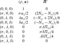
which yields the natural moment representation of the population as
 $$\begin{eqnarray}\displaystyle f_{(0,0,0)} & = & \displaystyle {\it\rho}(1-\unicode[STIX]{x1D61B}+M_{022}+M_{202}+M_{220}-M_{222}),\end{eqnarray}$$
 $$\begin{eqnarray}\displaystyle f_{({\it\sigma},0,0)} & = & \displaystyle {\textstyle \frac{1}{6}}{\it\rho} (\!3{\it\sigma}u_{x}+2N_{xz}-N_{yz}+\unicode[STIX]{x1D61B}-3{\it\sigma}M_{120}-3{\it\sigma}M_{102}+3{\it\sigma}M_{122}\nonumber\\ \displaystyle & & \displaystyle -\,3M_{202}-3M_{220}+3M_{222}\! ),\end{eqnarray}$$
 $$\begin{eqnarray}\displaystyle f_{(0,{\it\lambda},0)} & = & \displaystyle {\textstyle \frac{1}{6}}{\it\rho} (\!3{\it\lambda}u_{y}-N_{xz}+2N_{yz}+\unicode[STIX]{x1D61B}-3{\it\lambda}M_{210}-3{\it\lambda}M_{012}+3{\it\lambda}M_{212}\nonumber\\ \displaystyle & & \displaystyle -\,3M_{022}-3M_{220}+3M_{222}\! ),\end{eqnarray}$$
 $$\begin{eqnarray}\displaystyle f_{(0,0,{\it\delta})} & = & \displaystyle {\textstyle \frac{1}{6}}{\it\rho} (\!3{\it\delta}u_{z}-N_{xz}-N_{yz}+\unicode[STIX]{x1D61B}-3{\it\delta}M_{201}-3{\it\delta}M_{021}+3{\it\delta}M_{221}\nonumber\\ \displaystyle & & \displaystyle -\,3M_{022}-3M_{202}+3M_{222}\! ),\end{eqnarray}$$
 $$\begin{eqnarray}\displaystyle f_{({\it\sigma},{\it\lambda},0)} & = & \displaystyle {\textstyle \frac{1}{4}}{\it\rho}({\it\sigma}{\it\lambda}{\it\Pi}_{xy}+{\it\lambda}M_{210}+{\it\sigma}M_{120}+M_{220}-{\it\sigma}M_{122}-{\it\lambda}M_{212}-{\it\sigma}{\it\lambda}M_{112}-M_{222}),\nonumber\\ \displaystyle & & \displaystyle\end{eqnarray}$$
 $$\begin{eqnarray}\displaystyle f_{({\it\sigma},0,{\it\delta})} & = & \displaystyle {\textstyle \frac{1}{4}}{\it\rho}({\it\sigma}{\it\delta}{\it\Pi}_{xz}+{\it\delta}M_{201}+{\it\sigma}M_{102}+M_{202}-{\it\sigma}M_{122}-{\it\delta}M_{221}-{\it\sigma}{\it\delta}M_{121}-M_{222}),\nonumber\\ \displaystyle & & \displaystyle\end{eqnarray}$$
 $$\begin{eqnarray}\displaystyle f_{(0,{\it\lambda},{\it\delta})} & = & \displaystyle {\textstyle \frac{1}{4}}{\it\rho}({\it\lambda}{\it\delta}{\it\Pi}_{yz}+{\it\delta}M_{021}+{\it\lambda}M_{012}+M_{022}-{\it\lambda}M_{212}-{\it\delta}M_{221}-{\it\lambda}{\it\delta}M_{211}-M_{222}),\nonumber\\ \displaystyle & & \displaystyle\end{eqnarray}$$
 $$\begin{eqnarray}\displaystyle f_{({\it\sigma},{\it\lambda},{\it\delta})} & = & \displaystyle {\textstyle \frac{1}{8}}{\it\rho} (\!{\it\sigma}{\it\lambda}{\it\delta}M_{111}+{\it\sigma}M_{122}+{\it\lambda}M_{212}+{\it\delta}M_{221}+{\it\sigma}{\it\lambda}M_{112}+{\it\sigma}{\it\delta}M_{121}\nonumber\\ \displaystyle & & \displaystyle +\,{\it\lambda}{\it\delta}M_{211}+M_{222}\! ),\end{eqnarray}$$
 ${\it\sigma},{\it\lambda},{\it\gamma}\in \{-1,1\}$
, denotes the associated discrete velocity vector of the population. The model in the main text utilizes this representation and partitions it into three parts according to (2.6), where the shear part only includes the deviatoric stress tensor. The contribution of the locally conserved field
 $({\it\rho},\boldsymbol{u})$
and the deviatoric stress tensor
 $\boldsymbol{{\it\Pi}}^{\prime }$
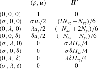
to the populations at unit density is summarized in table 2. Using this partition allows for the kinematic, the shear and the remaining higher-order moments to be relaxed according to (2.7).
Appendix B. Boundary conditions
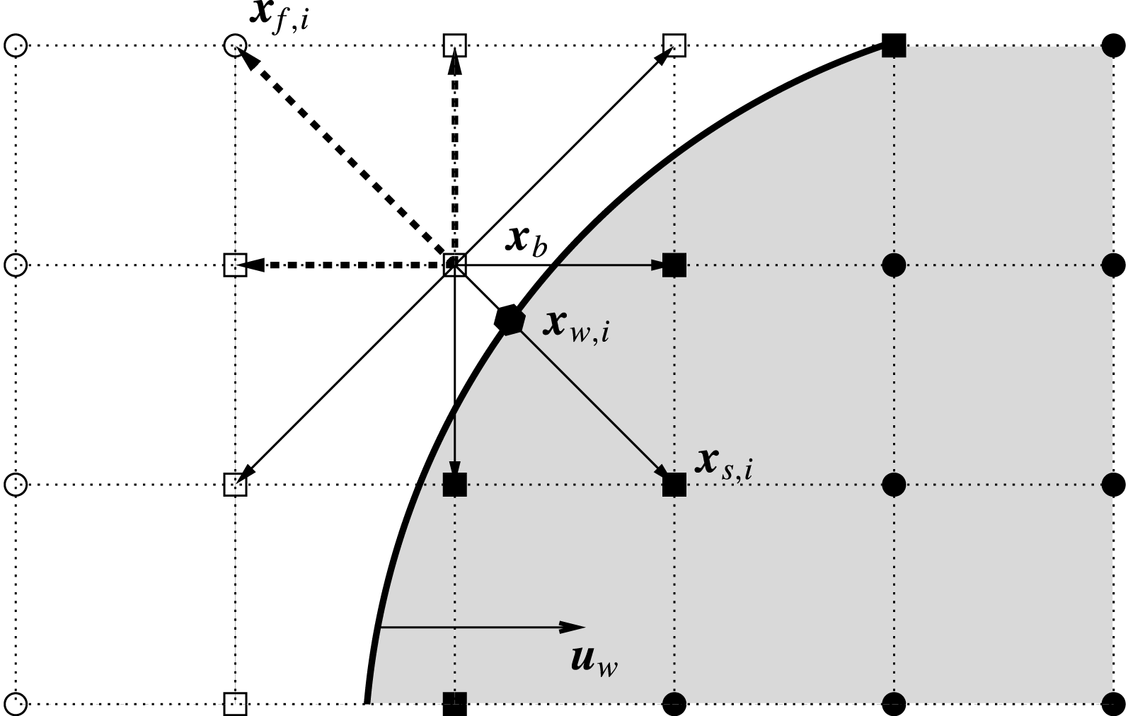
For the treatment of moving boundaries, let us consider figure 16. For the boundary node
 $\boldsymbol{x}_{b}$
in the fluid domain, the set of unknown populations
 $\bar{D}$
consists of the populations advected from the solid into the fluid region and are indicated by the dashed arrows in figure 16. Those missing populations are evaluated using Grad’s approximation as given by (2.13) using the target values
 $\boldsymbol{u}_{tgt}$
and
 ${\it\rho}_{tgt}$
and the pressure tensor is evaluated using a second-order finite difference scheme and the previous time-step values.
The unknown populations at the boundary node
 $\boldsymbol{x}_{b}$
are represented by the dashed arrows. ●: solid nodes; ○: fluid nodes; ▪: solid boundary nodes; ▫: fluid boundary nodes.

Contribution of the locally conserved fields and the deviatoric stress tensor to the populations at unit density.
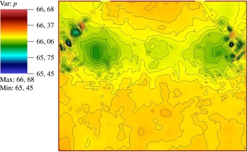
Instantaneous pressure
 $p^{\ast }=p/({\it\rho}v_{p,max})$
field slice and its contours at
 $90^{\circ }$
CA during the third cycle.

The momentum exerted from the object is accounted for by specifying an appropriate target velocity
 $\boldsymbol{u}_{tgt}$
at
 $\boldsymbol{x}_{b}$
, which may be obtained by an interpolation scheme involving the wall velocity
 $\boldsymbol{u}_{w,i}=\boldsymbol{u}(\boldsymbol{x}_{w,i},t)$
at the intersection point
 $\boldsymbol{x}_{w,i}$
and the velocities
 $\boldsymbol{u}_{f,i}=\boldsymbol{u}(\boldsymbol{x}_{f,i},t)$
at the adjacent fluid nodes
 $\boldsymbol{x}_{f,i}=\boldsymbol{x}_{b}+\boldsymbol{c}_{i}{\it\delta}_{t}$
for
 $i\in \bar{D}$
as shown in figure 16. Using an averaged linear interpolation for the target velocity yields
 $$\begin{eqnarray}\displaystyle \boldsymbol{u}_{tgt}=\frac{1}{n_{\bar{D}}}\mathop{\sum }_{i\in \bar{D}}\frac{q_{i}\boldsymbol{u}_{f,i}+\boldsymbol{u}_{w,i}}{1+q_{i}}, & & \displaystyle\end{eqnarray}$$
where
 $n_{\bar{D}}$
is the number of unknown populations and
 $q_{i}=\Vert \boldsymbol{x}_{b}-\boldsymbol{x}_{w,i}\Vert /\Vert \boldsymbol{c}_{i}\Vert$
. The target density is composed out of a static and dynamic part yielding
 $$\begin{eqnarray}\displaystyle {\it\rho}_{tgt}={\it\rho}_{stat}+{\it\rho}_{dyn} & & \displaystyle\end{eqnarray}$$
with
 $$\begin{eqnarray}\displaystyle & \displaystyle {\it\rho}_{stat}=\mathop{\sum }_{i\in \bar{D}}f_{i}^{bb}+\mathop{\sum }_{i\notin \bar{D}}f_{i}, & \displaystyle\end{eqnarray}$$
 $$\begin{eqnarray}\displaystyle & \displaystyle {\it\rho}_{dyn}=\mathop{\sum }_{i\in \bar{D}}6W_{i}{\it\rho}_{0}\boldsymbol{c}_{i}\boldsymbol{\cdot }\boldsymbol{u}_{w,i}, & \displaystyle\end{eqnarray}$$
where the static part
 ${\it\rho}_{stat}$
is the bounce-back density using the reflected populations
 $f_{i}^{bb}=\tilde{f}_{i}$
, where
 $\tilde{f}_{i}$
is associated with the velocity vector
 $\tilde{c}_{i}=-c_{i}$
. The dynamic part
 ${\it\rho}_{dyn}$
accounts for the density alteration by the mass displacement of the moving body, which may be derived by introducing a forcing term
 $F_{i}$
, which is necessary for the displacement. The mass and momentum conservation
 $$\begin{eqnarray}\displaystyle & \displaystyle \mathop{\sum }_{i\in \bar{D}}F_{i}=0 & \displaystyle\end{eqnarray}$$
 $$\begin{eqnarray}\displaystyle & \displaystyle \mathop{\sum }_{i\in \bar{D}}\boldsymbol{c}_{i}F_{i}={\it\rho}\boldsymbol{u}_{w}, & \displaystyle\end{eqnarray}$$
directly lead to
 $$\begin{eqnarray}\displaystyle F_{i}=6W_{i}{\it\rho}\boldsymbol{c}_{i}\boldsymbol{\cdot }\boldsymbol{u}_{w} & & \displaystyle\end{eqnarray}$$
for the
 $D3Q27$
-lattice, where the summation over all unknown populations in
 $\bar{D}$
yields the desired change in density.
As mentioned in the main text, the lattice sites uncovered by the moving object are reinitialized using the equilibrium distribution with the wall velocity and the local density average. To assert that no pressure waves are triggered at the boundary by the moving piston and such refill algorithm, figure 17 shows a slice of the pressure field with overlying pressure contours during the third cycle at its highest momentum at
 $90^{\circ }$
CA. It may be seen that the pressure field near the piston boundary appears to be smooth without spurious shocks.
In summary, this allows for a treatment of arbitrarily complex objects with second-order accuracy as shown in our previous work (Dorschner et al. Reference Dorschner, Chikatamarla, Bösch and Karlin2015).