1 Introduction
Flows in curved pipes have been the focus of much research over the last century, largely due to their prevalence in various fluid flow systems, with applications ranging from large-scale industrial piping systems to microscale biological flows. Flows with curved streamlines in general are known to produce secondary flows due to cross-stream pressure gradients resulting from centrifugal effects. These flows tend to be vortical in nature, and they continue to be areas of active research (Wang & Rusak Reference Wang and Rusak1997; Gallaire et al. Reference Gallaire, Ruith, Meiburg, Chomaz and Huerre2006; Ault et al. Reference Ault, Fani, Chen, Shin, Gallaire and Stone2016). Improved understanding of the velocity and pressure profiles in networks with curved piping elements can open the way for new applications, especially in physiology and heat and mass transfer.
In this paper, we study the flow development in the entry region of a curved pipe as well as the flow downstream of a curved pipe into a straight outlet. We identify scalings that eliminate dependence on the flow Reynolds number,
 $Re$
, and pipe-to-curvature radius ratio,
 $\unicode[STIX]{x1D6FC}$
, from linearized forms of the Navier–Stokes equations. We confirm these scalings using three-dimensional numerical simulations of the flows. Here, we define the Reynolds number as
 $Re=\unicode[STIX]{x1D70C}u_{avg}d/\unicode[STIX]{x1D707}$
, where
 $\unicode[STIX]{x1D70C}$
is the fluid density,
 $u_{avg}$
is the average axial pipe velocity,
 $d$
is the pipe diameter and
 $\unicode[STIX]{x1D707}$
is the dynamic viscosity of the fluid. The pipe-to-curvature radius ratio is defined as
 $\unicode[STIX]{x1D6FC}=d/(2R)$
, where
 $R$
is the radius of curvature of the centreline of the curved pipe. With these definitions, we define the Dean number as
 $D=Re^{2}\unicode[STIX]{x1D6FC}$
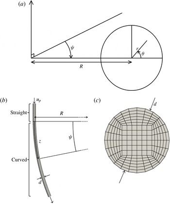
. Using a similar definition, Dean derived an analytical solution for fully developed pressure-driven flow in slowly curving pipes by rewriting the basic equations in toroidal coordinates (Dean Reference Dean1927, Reference Dean1928). We adopt a similar coordinate system, as shown in figure 1 for the entry problem, where
 $r$
and
 $\unicode[STIX]{x1D703}$
identify the position in the cross-section of the pipe and
 $\unicode[STIX]{x1D713}$
identifies the angular or axial position along the pipe. The corresponding arclength coordinate is given by
 $z$
. Dean’s work identified the presence of counter-rotating vortices in the fully developed flow in a curved pipe and has since inspired much research related to curved channels, including studies of the entry flow, unsteady laminar flows, flows in finite bends, channels with variable cross-sections, turbulent flows, the flow of non-Newtonian fluids, multiphase flows, mass transfer, fluid–particle mixtures, and many others (Berger, Talbot & Yao Reference Berger, Talbot and Yao1983).
Flow into a curved pipe of diameter
 $d$
with centreline radius of curvature
 $R$
. (a) The toroidal coordinate system used in the curved pipe section. (b,c) The top-down and axial cross-sectional views of the simulation domain respectively. It should be noted that
 $z$
is the centreline arclength corresponding to the angle
 $\unicode[STIX]{x1D713}$
. Each point is uniquely identified by (
 $r,\unicode[STIX]{x1D703},z$
). Arrows indicate the direction of flow. Mesh resolutions have been coarsened by a factor of 5 for visualization purposes. The inlet velocity is
 $u_{p}$
, denoting the fully developed parabolic flow in a straight pipe.

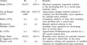
A review of studies related to the entry flow problem in curved pipes.

Several theoretical, experimental and numerical studies have documented features of developing flow in curved pipes. For a brief review of these studies, see table 1. Studies of the
 $O(d)$
region near the inlet show that the nature of the inlet condition significantly affects the initial development of the flow (Singh Reference Singh1974). A physical description of the flow development suggests that enhanced mixing due to secondary flows can significantly reduce hydrodynamic entrance lengths in comparison with those found in developing straight pipe flow for a given inlet condition (Singh Reference Singh1974), which we confirm numerically in § 4. Yao & Berger (Reference Yao and Berger1975) proposed an empirical relationship for the entry length
 $z_{ent}$
(non-dimensionalized by the pipe diameter) in a curved pipe, based upon the development length to reach 99 % of the fully developed flow velocity, which is given by
 $$\begin{eqnarray}z_{ent}=(3.8\unicode[STIX]{x1D6FC}+0.86)D^{1/4}\unicode[STIX]{x1D6FC}^{-1/2}\quad \text{for}~0.05<\unicode[STIX]{x1D6FC}<0.3.\end{eqnarray}$$
This result suggests that
 $z_{ent}\propto Re^{1/2}$
when
 $0.05<\unicode[STIX]{x1D6FC}<0.3$
. The majority of our simulations reported below are for
 $\unicode[STIX]{x1D6FC}<0.05$
, although we do observe the
 $z_{ent}\propto Re^{1/2}$
behaviour for our simulations with
 $\unicode[STIX]{x1D6FC}=0.1$
, albeit with a different scale factor from that suggested by (1.1) (see figure 3). The difference in prefactors is likely to be dependent on the inlet condition.
When
 $D\ll 1$
, then either
 $Re\ll 1$
,
 $\unicode[STIX]{x1D6FC}\ll 1$
, or both. If
 $Re\ll 1$
, the viscous flow develops over the geometric length scale of the pipe, and the entrance length is
 $O(d)$
(Mohanty & Asthana Reference Mohanty and Asthana1978; Fox, Pritchard & McDonald Reference Fox, Pritchard and McDonald2009). If
 $\unicode[STIX]{x1D6FC}\ll 1$
, and
 $D\ll 1$
, the flow is practically straight, and for a given
 $Re\gg 1$
the entrance length should be practically the same as in a straight pipe at the same Reynolds number with the same inlet condition, i.e. the entrance length should be
 $O(dRe)$
(Yao & Berger Reference Yao and Berger1975). Certainly, with uniform inlet flow, the entrance length in a straight pipe should be nearly identical to the entrance length in a curved pipe with
 $\unicode[STIX]{x1D6FC}\ll 1$
and
 $D\ll 1$
for the same
 $Re$
. However, for flow transitioning from a straight pipe to a curved pipe with
 $\unicode[STIX]{x1D6FC}\ll 1$
and
 $D\ll 1$
, the base flow is already fully developed, and the dynamics of interest is a small perturbation to the base flow. Thus, it is not immediately apparent that the perturbation dynamics also develops over
 $O(dRe)$
.
Several other studies have examined the nature of pipe flows into bends. Boutabaa et al. (Reference Boutabaa, Helin, Mompean and Thais2009) performed three-dimensional numerical simulations of developing flows in curved ducts for Newtonian and viscoelastic fluids (using the Phan-Thien–Tanner model) and found that the transition from two Dean cells to four occurs at a lower Dean number for viscoelastic fluids than for Newtonian fluids. Fairbank & So (Reference Fairbank and So1987) experimentally measured the upstream and downstream influences of a
 $180^{\circ }$
bend on a pipe flow, suggesting an upstream influence of one pipe diameter for
 $D=4.8\times 10^{4}$
and no upstream influence for
 $D=1.2\times 10^{4}$
. Furthermore, downstream influences of 14 and 11 pipe diameters were found for
 $D=4.8\times 10^{4}$
and
 $1.2\times 10^{4}$
respectively, indicating flow development more than twice as fast as predicted by the linearized
 $D\ll 1$
theory in § 3, which supports the physical description of flow development above. In addition, Olson & Snyder (Reference Olson and Snyder1985) presented experimental measurements of air flows in curved pipes with
 $1.0\times 10^{4}<D<2.5\times 10^{5}$
and showed that the secondary velocity components do not develop monotonically along the pipe, but instead overshoot before settling to their fully developed values. We show that this overshoot also occurs for Dean numbers at least in the range
 $O(0.1)<D<O(10^{4})$
, and can be described well by an asymptotic solution (see § 3). Liu & Masliyah (Reference Liu and Masliyah1996) also used numerical simulations to propose entrance length correlations for developing flow in helical pipes and also showed that the flow develops non-monotonically. Finally, Tadjfar & Smith (Reference Tadjfar and Smith2004) used slender-flow theory to develop models for the long-scale
 $O(dRe)$
flow in branching flows that match well with direct numerical simulations for a surprisingly large range of branching angles.
In addition, Smith (Reference Smith1976) studied the flow into a curved pipe with
 $Re\gg 1$
, primarily focusing attention on the
 $O(d)$
region from the inlet. He demonstrated that the influence of the region upstream of the bend is a vital factor in solving for the wall boundary layer solution in the curved pipe section and described a mechanism by which high-Reynolds-number pipe flows can adjust to disturbances downstream. Smith (Reference Smith1976) also briefly examined the
 $O(dRe)$
development of the flow and suggested that the problem needs a numerical treatment (see § 4.1 of Smith (Reference Smith1976)). Berger et al. (Reference Berger, Talbot and Yao1983) later suggested that it might be possible to obtain an analytical solution for this low-Dean-number entry flow problem using a perturbation approach, although, to the best of our knowledge, they never found such a solution. In addition to providing the numerical treatment that Smith (Reference Smith1976) suggests is necessary, we present an analytical solution to the problem originally posed by Berger et al. (Reference Berger, Talbot and Yao1983) for the flow in the limit of
 $D\ll 1$
, and we use the numerical simulations to show that this solution is valid up to
 $D=O(100)$
. Furthermore, although the upstream influence must be considered when obtaining the wall boundary layer solution for the
 $O(d)$
problem, Smith (Reference Smith1976) shows that for the long-length-scale
 $O(dRe)$
problem, the inlet condition will be practically the fully developed Poiseuille flow. This idea, introduced by Smith, makes the theory in § 3 possible, by providing a simple analytical boundary condition for both the entry and exit problems.
Previously, we considered the flow downstream of a curved pipe in a straight outlet section (Ault, Chen & Stone Reference Ault, Chen and Stone2015). In particular, we used scaling arguments to eliminate from the problem the dependence on the Reynolds number and upstream pipe curvature, and we systematically quantified the transition lengths as a function of
 $Re$
. Here, we apply similar scaling arguments to the developing flow in a curved pipe. We then reduce the governing equations to an eigenvalue problem for a sixth-order ordinary differential equation. By solving this problem, we arrive at an analytical solution for both the developing flow in a curved pipe and the flow downstream of a curved pipe in a straight outlet. For the latter case, we use cylindrical coordinates as in Ault et al. (Reference Ault, Chen and Stone2015), where
 $r$
and
 $\unicode[STIX]{x1D703}$
define the position on a cross-section and
 $z$
is the axial streamwise coordinate, where
 $z=0$
corresponds to the transition from the curved to straight pipe sections and
 $\unicode[STIX]{x1D703}=0$
points in the direction of the outer bend of the upstream curved section. It should be noted that we also use
 $z$
as the axial coordinate (arclength) in the developing curved pipe flow problem (figure 1).
In § 2 and appendix B, we provide details of the numerical approach used to verify our theoretical solutions. In § 3, we linearize the continuity and Navier–Stokes equations in toroidal or cylindrical coordinates and develop scaling arguments that eliminate
 $Re$
and
 $\unicode[STIX]{x1D6FC}$
dependence from the problems. We then use symmetry arguments and a separation of variables approach to achieve an analytical solution for both the developing curved pipe flow and the flow downstream of a curved pipe. We generalize these analyses to vector form in § 3.3. In § 4, we show that the identified scalings imply a linear relationship between the transition lengths and
 $Re$
, and we determine the theoretical proportionality coefficient for this relationship. Numerical simulation results are compared with the linearized theory of § 3, and the velocity/pressure data are seen to collapse when the scaling arguments are applied. We show that the proposed solutions match the numerical data well up to
 $D=O(100)$
and break down for larger Dean numbers. These results effectively address the questions originally posed by Smith (Reference Smith1976) and Berger et al. (Reference Berger, Talbot and Yao1983). Finally, in § 5, we present conclusions and ideas for future work.
2 Methods
In this section, we describe the flow geometry and the methodology used for determining transition lengths. Additional details about the numerical methods, including the specific flow solver and boundary conditions, can be found in appendix B.
2.1 Geometry
A sample simulation domain for the developing flow in a curved pipe is shown in figure 1(b,c). The domain consists of a straight inlet section with length
 $5d$
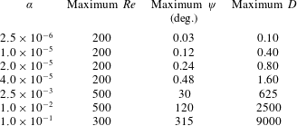
, which enters a curved pipe section that forms a circular arc. Properties of the simulations are given in table 2. The scaling arguments that will be developed in § 3 require
 $Re\gg 1$
and
 $D\ll 1$
. We choose values of
 $Re$
and
 $\unicode[STIX]{x1D6FC}$
that reasonably satisfy both of these limits, as well as constraints imposed by the solver. For the case of flow downstream of a curved pipe, similar simulations were performed (see Ault et al.
Reference Ault, Chen and Stone2015). Fully developed flow in a curved pipe was simulated entering a straight outlet, and the transition back to parabolic Poiseuille flow was studied.
Summary of geometric parameters used in the simulations for flow entering a curved pipe. The maximum value of
 $\unicode[STIX]{x1D713}$
denotes the total angle swept by the curved pipe section in the simulation domain. The total arclength of the curved section for each simulation was approximately 105 pipe diameters, except for the
 $\unicode[STIX]{x1D6FC}=1.0\times 10^{-1}$
case which had a total arclength of approximately 27 pipe diameters.

2.2 Determining transition/development lengths
We define the axial position at which a flow is fully developed as the axial coordinate,
 $z_{ent}$
, at which the magnitude of a component of the velocity or pressure has achieved 99 % of its final value. Lengths are non-dimensionalized by
 $d$
. We also specify a dimensionless entrance angle,
 $\unicode[STIX]{x1D713}_{ent}=2\unicode[STIX]{x1D6FC}z_{ent}$
, where
 $z_{ent}$
is the dimensionless arclength that is spanned by the angle
 $\unicode[STIX]{x1D713}_{ent}$
in radians. Subscript
 $D$
denotes the fully developed values in the curved pipe predicted by Dean (see (3.6)), and
 $u_{sec}=\sqrt{u_{r}^{2}+u_{\unicode[STIX]{x1D703}}^{2}}$
is the magnitude of the secondary velocity. To determine transition lengths, we examine a cross-section at
 $z=0$
(the entrance to the curved pipe) and determine the maximum values of
 $|u_{z}-u_{z,D}|$
,
 $|u_{sec}-u_{sec,D}|$
and
 $|p-p_{D}|$
. These represent deviations from the fully developed axial velocity component, secondary velocity component and pressure respectively. Systematically increasing
 $z$
in the axial direction, the maximum of each of these values is recorded for each
 $z$
. These perturbations decay monotonically over several orders of magnitude as
 $z$
is increased. However, we will show numerically and analytically that this transition is not monotonic and also contains a slowly oscillating component. Identifying the axial location where the chosen parameter achieves 99 % of its final value determines the entrance length
 $z_{ent}$
. This procedure is identical for the flow downstream of a curved pipe into a straight outlet, except that the parameters of interest are
 $|u_{z}-u_{p}|$
,
 $|u_{sec}|$
and
 $|p-p_{p}|$
, where the subscript
 $p$
denotes the fully developed Poiseuille flow.
3 Theory
In this section, we show that by linearizing the continuity and Navier–Stokes equations in toroidal and cylindrical coordinates about the respective fully developed flows, performing judicious scaling arguments and taking the asymptotic limits of small curvature and large Reynolds number, the
 $\unicode[STIX]{x1D6FC}$
and
 $Re$
dependence can be eliminated from the governing equations and boundary conditions for the perturbation pressure and velocity components. Symmetry arguments reduce the resulting equations to a single partial differential equation that is second order in the axial coordinate
 $z$
and sixth order in the transverse coordinate
 $r$
. Finally, a separation of variables approach results in an eigenvalue problem with a series solution of oscillating decaying exponentials in the axial direction.
3.1 Flow in a straight section downstream of a curved pipe
For both the entry and exit cases, the governing equations are the steady incompressible Navier–Stokes and continuity equations, given by
 $$\begin{eqnarray}\boldsymbol{u}\boldsymbol{\cdot }\unicode[STIX]{x1D735}\boldsymbol{u}=-\unicode[STIX]{x1D735}p+Re^{-1}\unicode[STIX]{x1D6FB}^{2}\boldsymbol{u}\quad \text{and}\quad \unicode[STIX]{x1D735}\boldsymbol{\cdot }\boldsymbol{u}=0,\end{eqnarray}$$
where
 $\boldsymbol{u}$
is the velocity vector non-dimensionalized by
 $u_{avg}$
and
 $p$
is the pressure non-dimensionalized by
 $\unicode[STIX]{x1D70C}u_{avg}^{2}$
. For the case of flow downstream of a curved pipe, we use cylindrical coordinates as in Ault et al. (Reference Ault, Chen and Stone2015). The components of the velocity vector are denoted
 $\boldsymbol{u}=(u_{r},u_{\unicode[STIX]{x1D703}},u_{z})$
, and the radial and axial coordinates
 $r$
and
 $z$
are non-dimensionalized by the pipe diameter
 $d$
. We linearize about the fully developed straight pipe solution (Poiseuille flow), so that
 $\boldsymbol{u}$
and
 $p$
are given by
 $$\begin{eqnarray}u_{r}=u_{r}^{\prime },\quad u_{\unicode[STIX]{x1D703}}=u_{\unicode[STIX]{x1D703}}^{\prime },\quad u_{z}=u_{p}(r)+u_{z}^{\prime },\quad p=p_{p}(z)+p^{\prime },\end{eqnarray}$$
where
 $u_{p}(r)=2-8r^{2}$
is the fully developed axial velocity component and
 $p_{p}(z)=-32z/Re+c$
is the fully developed pressure distribution (
 $c$
is a constant). Primes denote the small secondary components. Based upon the work of Dean (Reference Dean1927, Reference Dean1928) and Ault et al. (Reference Ault, Chen and Stone2015), we rescale the equations with
 $$\begin{eqnarray}\bar{z}=\frac{z}{Re},\quad \bar{p}^{\prime }=\frac{p^{\prime }}{\unicode[STIX]{x1D6FC}},\quad \bar{u}_{z}^{\prime }=\frac{u_{z}^{\prime }}{Re^{2}\unicode[STIX]{x1D6FC}},\quad \bar{u}_{r}^{\prime }=\frac{u_{r}^{\prime }}{Re\unicode[STIX]{x1D6FC}}\quad \text{and}\quad \bar{u}_{\unicode[STIX]{x1D703}}^{\prime }=\frac{u_{\unicode[STIX]{x1D703}}^{\prime }}{Re\unicode[STIX]{x1D6FC}}.\end{eqnarray}$$
In the asymptotic limits of
 $\unicode[STIX]{x1D6FC}\ll 1$
and
 $Re\gg 1$
, the governing equations (3.1) simplify to
 $$\begin{eqnarray}\displaystyle & \displaystyle \frac{\unicode[STIX]{x2202}\bar{u}_{r}^{\prime }}{\unicode[STIX]{x2202}r}+\frac{\bar{u}_{r}^{\prime }}{r}+\frac{1}{r}\frac{\unicode[STIX]{x2202}\bar{u}_{\unicode[STIX]{x1D703}}^{\prime }}{\unicode[STIX]{x2202}\unicode[STIX]{x1D703}}+\frac{\unicode[STIX]{x2202}\bar{u}_{z}^{\prime }}{\unicode[STIX]{x2202}\bar{z}}=0, & \displaystyle\end{eqnarray}$$
 $$\begin{eqnarray}\displaystyle & \displaystyle u_{p}\frac{\unicode[STIX]{x2202}\bar{u}_{r}^{\prime }}{\unicode[STIX]{x2202}\bar{z}}=-\frac{\unicode[STIX]{x2202}\bar{p}^{\prime }}{\unicode[STIX]{x2202}r}+\frac{1}{r}\frac{\unicode[STIX]{x2202}}{\unicode[STIX]{x2202}r}\left(r\frac{\unicode[STIX]{x2202}\bar{u}_{r}^{\prime }}{\unicode[STIX]{x2202}r}\right)+\frac{1}{r^{2}}\frac{\unicode[STIX]{x2202}^{2}\bar{u}_{r}^{\prime }}{\unicode[STIX]{x2202}\unicode[STIX]{x1D703}^{2}}-\frac{\bar{u}_{r}^{\prime }}{r^{2}}-\frac{2}{r^{2}}\frac{\unicode[STIX]{x2202}\bar{u}_{\unicode[STIX]{x1D703}}^{\prime }}{\unicode[STIX]{x2202}\unicode[STIX]{x1D703}}, & \displaystyle\end{eqnarray}$$
 $$\begin{eqnarray}\displaystyle & \displaystyle u_{p}\frac{\unicode[STIX]{x2202}\bar{u}_{\unicode[STIX]{x1D703}}^{\prime }}{\unicode[STIX]{x2202}\bar{z}}=-\frac{1}{r}\frac{\unicode[STIX]{x2202}\bar{p}^{\prime }}{\unicode[STIX]{x2202}\unicode[STIX]{x1D703}}+\frac{1}{r}\frac{\unicode[STIX]{x2202}}{\unicode[STIX]{x2202}r}\left(r\frac{\unicode[STIX]{x2202}\bar{u}_{\unicode[STIX]{x1D703}}^{\prime }}{\unicode[STIX]{x2202}r}\right)+\frac{1}{r^{2}}\frac{\unicode[STIX]{x2202}^{2}\bar{u}_{\unicode[STIX]{x1D703}}^{\prime }}{\unicode[STIX]{x2202}\unicode[STIX]{x1D703}^{2}}+\frac{2}{r^{2}}\frac{\unicode[STIX]{x2202}\bar{u}_{r}^{\prime }}{\unicode[STIX]{x2202}\unicode[STIX]{x1D703}}-\frac{\bar{u}_{\unicode[STIX]{x1D703}}^{\prime }}{r^{2}}, & \displaystyle\end{eqnarray}$$
 $$\begin{eqnarray}\displaystyle & \displaystyle \bar{u}_{r}^{\prime }\frac{\text{d}u_{p}}{\text{d}r}+u_{p}\frac{\unicode[STIX]{x2202}\bar{u}_{z}^{\prime }}{\unicode[STIX]{x2202}\bar{z}}=\frac{1}{r}\frac{\unicode[STIX]{x2202}}{\unicode[STIX]{x2202}r}\left(r\frac{\unicode[STIX]{x2202}\bar{u}_{z}^{\prime }}{\unicode[STIX]{x2202}r}\right)+\frac{1}{r^{2}}\frac{\unicode[STIX]{x2202}^{2}\bar{u}_{z}^{\prime }}{\unicode[STIX]{x2202}\unicode[STIX]{x1D703}^{2}}. & \displaystyle\end{eqnarray}$$
 $Re$
and
 $\unicode[STIX]{x1D6FC}$
.
3.2 Developing flow in a curved pipe
For the case of developing flow in a curved pipe, toroidal coordinates (figure 1 a) are used to represent the continuity and steady Navier–Stokes equations (Singh Reference Singh1974). These equations are given by
 $$\begin{eqnarray}\displaystyle & & \displaystyle \frac{\unicode[STIX]{x2202}u_{r}}{\unicode[STIX]{x2202}r}+\left(\frac{1+4\unicode[STIX]{x1D6FC}r\cos \unicode[STIX]{x1D703}}{1+2\unicode[STIX]{x1D6FC}r\cos \unicode[STIX]{x1D703}}\right)\frac{u_{r}}{r}+\frac{1}{r}\frac{\unicode[STIX]{x2202}u_{\unicode[STIX]{x1D703}}}{\unicode[STIX]{x2202}\unicode[STIX]{x1D703}}-\frac{2\unicode[STIX]{x1D6FC}u_{\unicode[STIX]{x1D703}}\sin \unicode[STIX]{x1D703}}{1+2\unicode[STIX]{x1D6FC}r\cos \unicode[STIX]{x1D703}}+\frac{1}{1+2\unicode[STIX]{x1D6FC}r\cos \unicode[STIX]{x1D703}}\frac{\unicode[STIX]{x2202}u_{z}}{\unicode[STIX]{x2202}z}=0,\nonumber\\ \displaystyle & & \displaystyle\end{eqnarray}$$
 $$\begin{eqnarray}\displaystyle & & \displaystyle \frac{u_{r}}{2}\frac{\unicode[STIX]{x2202}u_{r}}{\unicode[STIX]{x2202}r}+\frac{u_{\unicode[STIX]{x1D703}}}{2r}\frac{\unicode[STIX]{x2202}u_{r}}{\unicode[STIX]{x2202}\unicode[STIX]{x1D703}}+\frac{u_{z}}{2+4\unicode[STIX]{x1D6FC}r\cos \unicode[STIX]{x1D703}}\frac{\unicode[STIX]{x2202}u_{r}}{\unicode[STIX]{x2202}z}-\frac{u_{\unicode[STIX]{x1D703}}^{2}}{2r}-\frac{\unicode[STIX]{x1D6FC}u_{z}^{2}\cos \unicode[STIX]{x1D703}}{1+2\unicode[STIX]{x1D6FC}r\cos \unicode[STIX]{x1D703}}\nonumber\\ \displaystyle & & \displaystyle \quad =-\frac{1}{2}\frac{\unicode[STIX]{x2202}p}{\unicode[STIX]{x2202}r}-\frac{1}{Re}\left[\left(\frac{1}{2r}\frac{\unicode[STIX]{x2202}}{\unicode[STIX]{x2202}\unicode[STIX]{x1D703}}-\frac{\unicode[STIX]{x1D6FC}\sin \unicode[STIX]{x1D703}}{1+2\unicode[STIX]{x1D6FC}r\cos \unicode[STIX]{x1D703}}\right)\left(\frac{\unicode[STIX]{x2202}u_{\unicode[STIX]{x1D703}}}{\unicode[STIX]{x2202}r}+\frac{u_{\unicode[STIX]{x1D703}}}{r}-\frac{1}{r}\frac{\unicode[STIX]{x2202}u_{r}}{\unicode[STIX]{x2202}\unicode[STIX]{x1D703}}\right)\right.\nonumber\\ \displaystyle & & \displaystyle \qquad -\,\frac{1}{2\left(1+2\unicode[STIX]{x1D6FC}r\cos \unicode[STIX]{x1D703}\right)^{2}}\frac{\unicode[STIX]{x2202}^{2}u_{r}}{\unicode[STIX]{x2202}z^{2}}+\frac{1}{1+2\unicode[STIX]{x1D6FC}r\cos \unicode[STIX]{x1D703}}\nonumber\\ \displaystyle & & \displaystyle \qquad \left.\times \left(\frac{1}{2}\frac{\unicode[STIX]{x2202}^{2}u_{z}}{\unicode[STIX]{x2202}r\unicode[STIX]{x2202}z}+\frac{\unicode[STIX]{x1D6FC}\cos \unicode[STIX]{x1D703}}{1+2\unicode[STIX]{x1D6FC}r\cos \unicode[STIX]{x1D703}}\frac{\unicode[STIX]{x2202}u_{z}}{\unicode[STIX]{x2202}z}\right)\right],\end{eqnarray}$$
 $$\begin{eqnarray}\displaystyle & & \displaystyle \frac{u_{r}}{2}\frac{\unicode[STIX]{x2202}u_{\unicode[STIX]{x1D703}}}{\unicode[STIX]{x2202}r}+\frac{u_{\unicode[STIX]{x1D703}}}{2r}\frac{\unicode[STIX]{x2202}u_{\unicode[STIX]{x1D703}}}{\unicode[STIX]{x2202}\unicode[STIX]{x1D703}}+\frac{u_{z}}{2+4\unicode[STIX]{x1D6FC}r\cos \unicode[STIX]{x1D703}}\frac{\unicode[STIX]{x2202}u_{\unicode[STIX]{x1D703}}}{\unicode[STIX]{x2202}z}+\frac{u_{r}u_{\unicode[STIX]{x1D703}}}{2r}+\frac{\unicode[STIX]{x1D6FC}u_{z}^{2}\sin \unicode[STIX]{x1D703}}{1+2\unicode[STIX]{x1D6FC}r\cos \unicode[STIX]{x1D703}}=-\frac{1}{2r}\frac{\unicode[STIX]{x2202}p}{\unicode[STIX]{x2202}\unicode[STIX]{x1D703}}+\frac{1}{Re}\nonumber\\ \displaystyle & & \displaystyle \qquad \times \left[\frac{1}{2\left(1+2\unicode[STIX]{x1D6FC}r\cos \unicode[STIX]{x1D703}\right)^{2}}\frac{\unicode[STIX]{x2202}^{2}u_{\unicode[STIX]{x1D703}}}{\unicode[STIX]{x2202}z^{2}}-\frac{1}{r\left(2+4\unicode[STIX]{x1D6FC}r\cos \unicode[STIX]{x1D703}\right)}\frac{\unicode[STIX]{x2202}^{2}u_{z}}{\unicode[STIX]{x2202}z\unicode[STIX]{x2202}\unicode[STIX]{x1D703}}+\frac{\unicode[STIX]{x1D6FC}\sin \unicode[STIX]{x1D703}}{\left(1+2\unicode[STIX]{x1D6FC}r\cos \unicode[STIX]{x1D703}\right)^{2}}\frac{\unicode[STIX]{x2202}u_{z}}{\unicode[STIX]{x2202}z}\right.\nonumber\\ \displaystyle & & \displaystyle \qquad \left.+\left(\frac{1}{2}\frac{\unicode[STIX]{x2202}}{\unicode[STIX]{x2202}r}+\frac{\unicode[STIX]{x1D6FC}\cos \unicode[STIX]{x1D703}}{1+2\unicode[STIX]{x1D6FC}r\cos \unicode[STIX]{x1D703}}\right)\left(\frac{\unicode[STIX]{x2202}u_{\unicode[STIX]{x1D703}}}{\unicode[STIX]{x2202}r}+\frac{u_{\unicode[STIX]{x1D703}}}{r}-\frac{1}{r}\frac{\unicode[STIX]{x2202}u_{r}}{\unicode[STIX]{x2202}\unicode[STIX]{x1D703}}\right)\right],\end{eqnarray}$$
 $$\begin{eqnarray}\displaystyle & & \displaystyle \frac{u_{r}}{2}\frac{\unicode[STIX]{x2202}u_{z}}{\unicode[STIX]{x2202}r}+\frac{\unicode[STIX]{x1D6FC}u_{r}u_{z}\cos \unicode[STIX]{x1D703}}{1+2\unicode[STIX]{x1D6FC}r\cos \unicode[STIX]{x1D703}}+\frac{u_{\unicode[STIX]{x1D703}}}{2r}\frac{\unicode[STIX]{x2202}u_{z}}{\unicode[STIX]{x2202}\unicode[STIX]{x1D703}}-\frac{\unicode[STIX]{x1D6FC}u_{\unicode[STIX]{x1D703}}u_{z}\sin \unicode[STIX]{x1D703}}{1+2\unicode[STIX]{x1D6FC}r\cos \unicode[STIX]{x1D703}}+\frac{u_{z}}{2+4\unicode[STIX]{x1D6FC}r\cos \unicode[STIX]{x1D703}}\frac{\unicode[STIX]{x2202}u_{z}}{\unicode[STIX]{x2202}z}\nonumber\\ \displaystyle & & \displaystyle \qquad =-\frac{1}{2+4\unicode[STIX]{x1D6FC}r\cos \unicode[STIX]{x1D703}}\frac{\unicode[STIX]{x2202}p}{\unicode[STIX]{x2202}z}+\frac{1}{Re}\left[\left(\frac{\unicode[STIX]{x2202}}{\unicode[STIX]{x2202}r}+\frac{1}{r}\right)\left(\frac{1}{2}\frac{\unicode[STIX]{x2202}u_{z}}{\unicode[STIX]{x2202}r}+\frac{\unicode[STIX]{x1D6FC}u_{z}\cos \unicode[STIX]{x1D703}}{1+2\unicode[STIX]{x1D6FC}r\cos \unicode[STIX]{x1D703}}\right)\right.\nonumber\\ \displaystyle & & \displaystyle \qquad \left.+\frac{1}{2r^{2}}\frac{\unicode[STIX]{x2202}^{2}u_{z}}{\unicode[STIX]{x2202}\unicode[STIX]{x1D703}^{2}}-\frac{\unicode[STIX]{x1D6FC}}{r}\frac{\unicode[STIX]{x2202}}{\unicode[STIX]{x2202}\unicode[STIX]{x1D703}}\left(\frac{u_{z}\sin \unicode[STIX]{x1D703}}{1+2\unicode[STIX]{x1D6FC}r\cos \unicode[STIX]{x1D703}}\right)-\left(\frac{\unicode[STIX]{x2202}}{\unicode[STIX]{x2202}r}+\frac{1}{r}\right)\frac{1}{2+4\unicode[STIX]{x1D6FC}r\cos \unicode[STIX]{x1D703}}\frac{\unicode[STIX]{x2202}u_{r}}{\unicode[STIX]{x2202}z}\right.\nonumber\\ \displaystyle & & \displaystyle \qquad \left.-\frac{1}{r}\frac{\unicode[STIX]{x2202}}{\unicode[STIX]{x2202}\unicode[STIX]{x1D703}}\left(\frac{1}{2+4\unicode[STIX]{x1D6FC}r\cos \unicode[STIX]{x1D703}}\frac{\unicode[STIX]{x2202}u_{\unicode[STIX]{x1D703}}}{\unicode[STIX]{x2202}z}\right)\right].\end{eqnarray}$$
 $$\begin{eqnarray}\displaystyle & \displaystyle u_{r,D}(r,\unicode[STIX]{x1D703})=Re\unicode[STIX]{x1D6FC}\cos \unicode[STIX]{x1D703}f_{1}(r)=u_{r,D}^{\prime }(r,\unicode[STIX]{x1D703}), & \displaystyle\end{eqnarray}$$
 $$\begin{eqnarray}\displaystyle & \displaystyle u_{\unicode[STIX]{x1D703},D}(r,\unicode[STIX]{x1D703})=-Re\unicode[STIX]{x1D6FC}\sin \unicode[STIX]{x1D703}f_{2}(r)=u_{\unicode[STIX]{x1D703},D}^{\prime }(r,\unicode[STIX]{x1D703}), & \displaystyle\end{eqnarray}$$
 $$\begin{eqnarray}\displaystyle & \displaystyle u_{z,D}(r,\unicode[STIX]{x1D703})=f_{3}(r)-\unicode[STIX]{x1D6FC}\cos \unicode[STIX]{x1D703}f_{4}(r)+Re^{2}\unicode[STIX]{x1D6FC}\cos \unicode[STIX]{x1D703}f_{5}(r)=u_{p}(r)+u_{z,D}^{\prime }(r,\unicode[STIX]{x1D703}), & \displaystyle\end{eqnarray}$$
 $$\begin{eqnarray}\displaystyle & \displaystyle p_{D}(r,\unicode[STIX]{x1D703},z)=-\frac{32z}{Re}+\unicode[STIX]{x1D6FC}\cos \unicode[STIX]{x1D703}f_{6}(r)+c=p_{p}(z)+p_{D}^{\prime }(r,\unicode[STIX]{x1D703}), & \displaystyle\end{eqnarray}$$
 $D$
subscript denotes Dean’s solution. It should be noted that this solution is strictly valid in the limit
 $D\ll 1$
. The
 $f_{i}(r)$
are polynomials in
 $r$
given by
 $$\begin{eqnarray}\displaystyle & \displaystyle f_{1}(r)={\textstyle \frac{1}{36}}\left(1-4r^{2}\right)^{2}\left(1-r^{2}\right), & \displaystyle\end{eqnarray}$$
 $$\begin{eqnarray}\displaystyle & \displaystyle f_{2}(r)={\textstyle \frac{1}{144}}\left(1-4r^{2}\right)\left(4-92r^{2}+112r^{4}\right), & \displaystyle\end{eqnarray}$$
 $$\begin{eqnarray}\displaystyle & \displaystyle f_{3}(r)=u_{p}(r)=2-8r^{2}, & \displaystyle\end{eqnarray}$$
 $$\begin{eqnarray}\displaystyle & \displaystyle f_{4}(r)=3r\left(1-4r^{2}\right), & \displaystyle\end{eqnarray}$$
 $$\begin{eqnarray}\displaystyle & \displaystyle f_{5}(r)=\frac{r}{2880}\left(1-4r^{2}\right)\left(19-84r^{2}+144r^{4}-64r^{6}\right), & \displaystyle\end{eqnarray}$$
 $$\begin{eqnarray}\displaystyle & \displaystyle f_{6}(r)=\frac{r}{3}\left(18-48r^{2}+64r^{4}\right). & \displaystyle\end{eqnarray}$$
 $\unicode[STIX]{x1D6FC}\ll 1$
and
 $Re\gg 1$
, the disturbance part of Dean’s solution can be written as
 $$\begin{eqnarray}\displaystyle \left.\begin{array}{@{}c@{}}\displaystyle \bar{u}_{r,D}^{\prime }(r,\unicode[STIX]{x1D703})=\cos \unicode[STIX]{x1D703}f_{1}(r),\quad \bar{u}_{\unicode[STIX]{x1D703},D}^{\prime }(r,\unicode[STIX]{x1D703})=-\sin \unicode[STIX]{x1D703}f_{2}(r),\\ \displaystyle \bar{u}_{z,D}^{\prime }(r,\unicode[STIX]{x1D703})=\cos \unicode[STIX]{x1D703}f_{5}(r),\quad \bar{p}_{D}^{\prime }(r,\unicode[STIX]{x1D703})=\cos \unicode[STIX]{x1D703}f_{6}(r).\end{array}\right\} & & \displaystyle\end{eqnarray}$$
We now linearize about Dean’s analytical solution in a curved pipe as
 $$\begin{eqnarray}u_{r}=u_{r,D}+u_{r}^{\prime },\quad u_{\unicode[STIX]{x1D703}}=u_{\unicode[STIX]{x1D703},D}+u_{\unicode[STIX]{x1D703}}^{\prime },\quad u_{z}=u_{z,D}+u_{z}^{\prime }\quad \text{and}\quad p=p_{D}+p^{\prime }.\end{eqnarray}$$
Using this linearization along with the scalings (3.3), the governing equations (3.5) reduce to exactly the same form as equation (3.4) in the limits
 $\unicode[STIX]{x1D6FC}\ll 1$
and
 $Re\gg 1$
. Thus, the developing flow in a curved pipe and the flow downstream of a curved pipe in a straight outlet can both be represented with the same form of governing equations, where the linearization is about the fully developed Poiseuille flow for the flow downstream of a curved pipe, and the linearization is about Dean’s solution for the developing flow in a curved pipe.
3.3 Vector form
Perhaps a simpler way to see the equivalence between the two flow problems is by working with the vector forms of the equations. We use the same notations as before, where
 $z$
is understood to be the pipe centreline coordinate, which is generally curved, and
 $r,\unicode[STIX]{x1D703}$
are spatial coordinates on the cross-section. The gradient operator
 $\unicode[STIX]{x1D735}$
can be written as
 $$\begin{eqnarray}\unicode[STIX]{x1D735}=\frac{\boldsymbol{e}_{z}}{1+2\unicode[STIX]{x1D6FC}r\cos \unicode[STIX]{x1D703}}\frac{\unicode[STIX]{x2202}}{\unicode[STIX]{x2202}z}+\unicode[STIX]{x1D735}_{\bot }\end{eqnarray}$$
for a pipe with constant curvature, where
 $\unicode[STIX]{x1D735}_{\bot }$
corresponds to a gradient in the plane normal to the pipe axis, i.e.
 $\boldsymbol{e}_{z}\boldsymbol{\cdot }\,\unicode[STIX]{x1D735}_{\bot }=0$
. The velocity vector is written
 $\boldsymbol{u}=\boldsymbol{u}_{D}+\boldsymbol{u}^{\prime }$
as in § 3.2. We also write
 $\boldsymbol{u}^{\prime }=\boldsymbol{u}_{\bot }^{\prime }+\boldsymbol{e}_{z}u_{z}^{\prime }$
. Neglecting terms quadratic in
 $\boldsymbol{u}^{\prime }$
, the Navier–Stokes equations are
 $$\begin{eqnarray}\boldsymbol{u}_{D}\boldsymbol{\cdot }\unicode[STIX]{x1D735}\boldsymbol{u}_{D}+\boldsymbol{u}_{D}\boldsymbol{\cdot }\unicode[STIX]{x1D735}\boldsymbol{u}^{\prime }+\boldsymbol{u}^{\prime }\boldsymbol{\cdot }\unicode[STIX]{x1D735}\boldsymbol{u}_{D}=-\unicode[STIX]{x1D735}p_{D}-\unicode[STIX]{x1D735}p^{\prime }+\frac{1}{Re}\unicode[STIX]{x1D6FB}^{2}\boldsymbol{u}_{D}+\frac{1}{Re}\unicode[STIX]{x1D6FB}^{2}\boldsymbol{u}^{\prime },\end{eqnarray}$$
where
 $\boldsymbol{u}_{D}=\boldsymbol{u}_{p}+\boldsymbol{u}_{D}^{\prime }$
. We consider only the leading effects of pipe curvature, i.e. we retain terms up to
 $O(\unicode[STIX]{x1D6FC}u_{p})$
and
 $O(\unicode[STIX]{x1D6FC}^{0}|\boldsymbol{u}^{\prime }|)$
. For
 $\unicode[STIX]{x1D6FC}\ll 1$
, (3.11) becomes
 $$\begin{eqnarray}u_{p}\frac{\unicode[STIX]{x2202}u_{z}^{\prime }}{\unicode[STIX]{x2202}z}\boldsymbol{e}_{z}+u_{p}\frac{\unicode[STIX]{x2202}\boldsymbol{u}_{\bot }^{\prime }}{\unicode[STIX]{x2202}z}+\boldsymbol{u}_{\bot }^{\prime }\boldsymbol{\cdot }\unicode[STIX]{x1D735}_{\bot }u_{p}\boldsymbol{e}_{z}=-\unicode[STIX]{x1D735}_{\bot }p^{\prime }-\frac{\unicode[STIX]{x2202}p^{\prime }}{\unicode[STIX]{x2202}z}\boldsymbol{e}_{z}+\frac{1}{Re}\unicode[STIX]{x1D6FB}^{2}\boldsymbol{u}_{\bot }^{\prime }+\frac{1}{Re}\unicode[STIX]{x1D6FB}^{2}u_{z}^{\prime }\boldsymbol{e}_{z}.\end{eqnarray}$$
The boundary conditions for the flow (§ 3.4) determine that the scaling for the perturbation must be the same as the scaling for the fully developed flow, which suggests
 $|\boldsymbol{u}_{\bot }^{\prime }|=O(\unicode[STIX]{x1D6FC}Re)$
,
 $p^{\prime }=O(\unicode[STIX]{x1D6FC})$
and
 $|u_{z}^{\prime }|=O(\unicode[STIX]{x1D6FC}Re^{2})$
. For the developing flow, continuity suggests that the flow evolves on a length scale
 $z=O(Re)$
, confirming the scalings (3.3). Applying these scalings to (3.12) and considering the limit
 $Re\gg 1$
gives
 $$\begin{eqnarray}u_{p}\frac{\unicode[STIX]{x2202}\bar{\boldsymbol{u}}_{\bot }^{\prime }}{\unicode[STIX]{x2202}\bar{z}}+u_{p}\frac{\unicode[STIX]{x2202}\bar{u}_{z}^{\prime }}{\unicode[STIX]{x2202}\bar{z}}\boldsymbol{e}_{z}+\bar{u}_{r}^{\prime }\frac{\text{d}u_{p}}{\text{d}r}\boldsymbol{e}_{z}=-\unicode[STIX]{x1D735}_{\bot }\bar{p}^{\prime }+\unicode[STIX]{x1D6FB}_{\bot }^{2}\bar{\boldsymbol{u}}_{\bot }^{\prime }+\unicode[STIX]{x1D6FB}_{\bot }^{2}\bar{u}_{z}^{\prime }\boldsymbol{e}_{z},\end{eqnarray}$$
which is exactly the vector form of (3.4). If the pipe is straight and the flow is instead linearized about the fully developed Poiseuille flow, (3.13) will be exactly the same; see § 3.1 for the details. Therefore, both the developing flow in a curved pipe and the flow downstream of a curved pipe satisfy the same governing equations.
3.4 Boundary conditions
Next, we consider the boundary conditions for each problem. For the developing flow in a curved pipe, the flow approaches Dean’s analytical solution, and for the case of flow downstream of a curved pipe, the flow approaches the fully developed Poiseuille flow. For both cases, these conditions imply
 $$\begin{eqnarray}\bar{\boldsymbol{u}}^{\prime }\rightarrow \mathbf{0}\quad \text{and}\quad \bar{p}^{\prime }\rightarrow 0,\quad \text{as}~\bar{z}\rightarrow \infty .\end{eqnarray}$$
In addition, the no-slip boundary condition at the pipe wall requires
 $$\begin{eqnarray}\bar{\boldsymbol{u}}^{\prime }=\mathbf{0}\quad \text{at}~r=1/2\end{eqnarray}$$
for both cases.
Finally, we consider the inlet conditions at
 $\bar{z}=0$
. As mentioned above, Smith (Reference Smith1976) analysed the inlet region in a curved pipe for
 $Re\gg 1$
and demonstrated that in order to solve the
 $O(1)$
boundary layer problem, a consideration of the upstream influence is necessary. However, Smith also stated that the upstream influence is practically negligible in the core, and thus for the
 $O(Re)$
problem, the inlet boundary condition is practically the fully developed Poiseuille flow. By analogy, for the case of flow downstream of a curved pipe, we claim, and verify numerically below, that the inlet boundary condition should be practically the fully developed curved pipe solution of Dean. For the developing flow in a curved pipe, we then have
 $$\begin{eqnarray}\boldsymbol{u}^{\prime }=\boldsymbol{u}_{p}-\boldsymbol{u}_{D}\quad \text{and}\quad p^{\prime }=p_{p}-p_{D}\quad \text{at}~\bar{z}=0,\end{eqnarray}$$
while we have
 $$\begin{eqnarray}\boldsymbol{u}^{\prime }=\boldsymbol{u}_{D}-\boldsymbol{u}_{p}\quad \text{and}\quad p^{\prime }=p_{D}-p_{p}\quad \text{at}~\bar{z}=0\end{eqnarray}$$
for the flow downstream of fully developed curved pipe flow.
Having shown that the developing flow in a curved pipe and the flow downstream of a curved pipe both satisfy the same governing equations (with the appropriate linearizations), we now also see that both flows satisfy the same boundary conditions, up to a factor of
 $-1$
in the inlet condition. Thus, the solution to (3.4), subject to the boundary conditions (3.14), (3.15) and (3.17), simultaneously gives the solution for both problems. These solutions are strictly valid in the limits
 $D\ll 1$
and
 $Re\gg 1$
(which implies
 $\unicode[STIX]{x1D6FC}\ll 1$
). The limit
 $D\ll 1$
is required to apply Dean’s analytical solution (3.6). However, in § 4 we use numerical solutions to show that the solution accurately predicts transition lengths to within
 ${\sim}5\,\%$
for laminar flows with
 $D\leqslant 100$
and
 $Re\geqslant 50$
. We also confirm the scaling arguments by showing that the velocity and pressure perturbations collapse after rescaling the data with (3.3) for a range of
 $Re$
and
 $\unicode[STIX]{x1D6FC}$
.
3.5 Separation of variables solution
To begin with, we present additional theoretical considerations that allow an analytical solution to the governing equations to be developed. The results are achieved with a combination of symmetry arguments and a separation of variables approach. It should be noted that the inlet boundary condition (3.17) has the symmetry property that
 $\bar{u}_{r}^{\prime }$
,
 $\bar{u}_{z}^{\prime }$
and
 $\bar{p}^{\prime }$
all have a
 $\cos \unicode[STIX]{x1D703}$
dependence, while
 $\bar{u}_{\unicode[STIX]{x1D703}}^{\prime }$
has a
 $\sin \unicode[STIX]{x1D703}$
dependence. Due to linearity, we assume that the transitioning flow maintains this symmetry condition throughout its development, and we define new primary variables
 $U_{r}$
,
 $U_{\unicode[STIX]{x1D703}}$
,
 $U_{z}$
and
 $P$
, such that
 $$\begin{eqnarray}\displaystyle \left.\begin{array}{@{}c@{}}\displaystyle \bar{u}_{r}^{\prime }(r,\unicode[STIX]{x1D703},\bar{z})=\cos \unicode[STIX]{x1D703}\,U_{r}(r,\bar{z}),\quad \bar{u}_{\unicode[STIX]{x1D703}}^{\prime }(r,\unicode[STIX]{x1D703},\bar{z})=\sin \unicode[STIX]{x1D703}\,U_{\unicode[STIX]{x1D703}}(r,\bar{z}),\\ \displaystyle \bar{u}_{z}^{\prime }(r,\unicode[STIX]{x1D703},\bar{z})=\cos \unicode[STIX]{x1D703}\,U_{z}(r,\bar{z}),\quad \bar{p}^{\prime }(r,\unicode[STIX]{x1D703},\bar{z})=\cos \unicode[STIX]{x1D703}\,P(r,\bar{z}).\end{array}\right\} & & \displaystyle\end{eqnarray}$$
Now, the governing equations (3.4) become
 $$\begin{eqnarray}\displaystyle & \displaystyle \frac{1}{r}\frac{\unicode[STIX]{x2202}}{\unicode[STIX]{x2202}r}\left(rU_{r}\right)+\frac{U_{\unicode[STIX]{x1D703}}}{r}+\frac{\unicode[STIX]{x2202}U_{z}}{\unicode[STIX]{x2202}\bar{z}}=0, & \displaystyle\end{eqnarray}$$
 $$\begin{eqnarray}\displaystyle & \displaystyle u_{p}\frac{\unicode[STIX]{x2202}U_{r}}{\unicode[STIX]{x2202}\bar{z}}=-\frac{\unicode[STIX]{x2202}P}{\unicode[STIX]{x2202}r}+\frac{1}{r}\frac{\unicode[STIX]{x2202}}{\unicode[STIX]{x2202}r}\left(r\frac{\unicode[STIX]{x2202}U_{r}}{\unicode[STIX]{x2202}r}\right)-\frac{2U_{r}}{r^{2}}-\frac{2U_{\unicode[STIX]{x1D703}}}{r^{2}}, & \displaystyle\end{eqnarray}$$
 $$\begin{eqnarray}\displaystyle & \displaystyle u_{p}\frac{\unicode[STIX]{x2202}U_{\unicode[STIX]{x1D703}}}{\unicode[STIX]{x2202}\bar{z}}=\frac{P}{r}+\frac{1}{r}\frac{\unicode[STIX]{x2202}}{\unicode[STIX]{x2202}r}\left(r\frac{\unicode[STIX]{x2202}U_{\unicode[STIX]{x1D703}}}{\unicode[STIX]{x2202}r}\right)-\frac{2U_{r}}{r^{2}}-\frac{2U_{\unicode[STIX]{x1D703}}}{r^{2}}, & \displaystyle\end{eqnarray}$$
 $$\begin{eqnarray}\displaystyle & \displaystyle U_{r}\frac{\text{d}u_{p}}{\text{d}r}+u_{p}\frac{\unicode[STIX]{x2202}U_{z}}{\unicode[STIX]{x2202}\bar{z}}=\frac{1}{r}\frac{\unicode[STIX]{x2202}}{\unicode[STIX]{x2202}r}\left(r\frac{\unicode[STIX]{x2202}U_{z}}{\unicode[STIX]{x2202}r}\right)-\frac{U_{z}}{r^{2}}. & \displaystyle\end{eqnarray}$$
Next,
 $U_{r}$
,
 $U_{\unicode[STIX]{x1D703}}$
and
 $P$
can be eliminated from (3.19), resulting in a partial differential equation for
 $U_{z}$
given by
 $$\begin{eqnarray}\displaystyle & & \displaystyle \frac{\unicode[STIX]{x2202}}{\unicode[STIX]{x2202}\bar{z}^{2}}\left(u_{p}^{2}\,{\mathcal{L}}(rU_{z})+2ru_{p}\frac{\text{d}u_{p}}{\text{d}r}\frac{\unicode[STIX]{x2202}U_{z}}{\unicode[STIX]{x2202}r}\right)-\frac{\unicode[STIX]{x2202}}{\unicode[STIX]{x2202}\bar{z}}\left(2u_{p}\,{\mathcal{L}}^{2}(rU_{z})+4\frac{\text{d}u_{p}}{\text{d}r}\frac{\unicode[STIX]{x2202}}{\unicode[STIX]{x2202}r}\left({\mathcal{L}}(rU_{z})\right)\right)\nonumber\\ \displaystyle & & \displaystyle \qquad +\,{\mathcal{L}}^{3}(rU_{z})=0,\end{eqnarray}$$
where
 ${\mathcal{L}}$
is the linear operator
 ${\mathcal{L}}=r(\unicode[STIX]{x2202}/\unicode[STIX]{x2202}r)((1/r)(\unicode[STIX]{x2202}/\unicode[STIX]{x2202}r))$
. It should be recalled that
 $u_{p}(r)=2-8r^{2}$
. Examining the structure of (3.20), we assume a solution of the form
 $$\begin{eqnarray}U_{z}(r,\bar{z})=\mathop{\sum }_{n=1}^{\infty }a_{n}F_{n}(r)\text{e}^{-k_{n}\bar{z}},\end{eqnarray}$$
which results in a sixth-order ordinary differential equation eigenvalue problem for the eigenvalues
 $k_{n}$
of the form
 $$\begin{eqnarray}\displaystyle & & \displaystyle k_{n}^{2}\left(u_{p}^{2}\,{\mathcal{L}}(rF_{n})+2ru_{p}\frac{\text{d}u_{p}}{\text{d}r}\frac{\text{d}F_{n}}{\text{d}r}\right)+k_{n}\left(2u_{p}\,{\mathcal{L}}^{2}(rF_{n})+4\frac{\text{d}u_{p}}{\text{d}r}\frac{\text{d}}{\text{d}r}\left({\mathcal{L}}\left(rF_{n}\right)\right)\right)\nonumber\\ \displaystyle & & \displaystyle \qquad +\,{\mathcal{L}}^{3}(rF_{n})=0.\end{eqnarray}$$
Boundedness of pressure and velocity at the origin requires
 $$\begin{eqnarray}F_{n}=\frac{\text{d}^{2}F_{n}}{\text{d}r^{2}}=\frac{\text{d}^{4}F_{n}}{\text{d}r^{4}}=0\quad \text{at}~r=0.\end{eqnarray}$$
The no-slip condition at the pipe wall (
 $r=1/2$
) requires
 $U_{r}(1/2,\bar{z})=U_{\unicode[STIX]{x1D703}}(1/2,\bar{z})=U_{z}(1/2,\bar{z})=0$
. In terms of the
 $F_{n}(r)$
, these conditions require
 $$\begin{eqnarray}F_{n}=0,\quad \frac{\text{d}F_{n}}{\text{d}r}=-\frac{1}{2}\frac{\text{d}^{2}F_{n}}{\text{d}r^{2}}\quad \text{and}\quad \frac{\text{d}^{2}F_{n}}{\text{d}r^{2}}=-\frac{1}{6}\frac{\text{d}^{3}F_{n}}{\text{d}r^{3}}\quad \text{at}~r=1/2.\end{eqnarray}$$
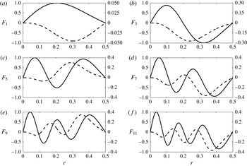
Thus, we have a sixth-order ordinary differential equation (3.22) subject to the six boundary conditions (3.23) and (3.24). A combined Taylor series expansion/shooting approach is used to solve the ordinary differential equation (3.22) and is described in detail in appendix A. The
 $F_{n}(r)$
corresponding to the
 $k_{n}$
with positive imaginary components are plotted in figure 2, renormalized such that the maximum value of their real parts is one. It should be noted that eigenvalues and eigenfunctions come in complex pairs, i.e.
 $\{k_{2},F_{2}(r)\}=\{k_{1}^{\ast },F_{1}^{\ast }(r)\}$
, where the
 $^{\ast }$
indicates the complex conjugate.
Representative eigenfunctions in the series solution (3.21) to the ordinary differential equation (3.22) subject to (3.23) and (3.24): (a)
 $F_{1}(r)$
, (b)
 $F_{3}(r)$
, (c)
 $F_{5}(r)$
, (d)
 $F_{7}(r)$
, (e)
 $F_{9}(r)$
, (f)
 $F_{11}(r)$
. Solid lines denote the real parts of the eigenfunctions (left axis) and dashed lines denote the imaginary parts of the eigenfunctions (right axis). Here, the eigenfunctions have been renormalized such that the maximum absolute value of their real part is one.

Entrance lengths,
 $z_{ent}$
, for developing flow in a curved pipe, non-dimensionalized by
 $d$
, for various
 $\unicode[STIX]{x1D6FC}$
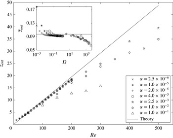
. The data show a good fit with the theoretical prediction (4.1) from § 3 for
 $D<O(100)$
. As
 $D$
increases to
 $O(100)$
, enhanced secondary flow reduces the entrance length with respect to the theoretical linear relationship for
 $D\ll 1$
. The inset shows the rescaled
 $\bar{z}_{ent}$
versus
 $D$
. The maximum relative error between theory and numerics is less than
 ${\sim}5\,\%$
for
 $D\leqslant 100$
and
 $Re\geqslant 50$
.

Finally, the series coefficients
 $\{a_{n}\}$
in (3.21) can be determined using the boundary condition
 $\bar{u}_{z}^{\prime }(r,\unicode[STIX]{x1D703},\bar{z}=0)=\cos \unicode[STIX]{x1D703}f_{5}(r)$
, which gives
 $U_{z}(r,\bar{z}=0)=f_{5}(r)$
. In terms of (3.21), this condition requires
 $$\begin{eqnarray}\mathop{\sum }_{n=1}^{\infty }a_{n}F_{n}(r)=f_{5}(r).\end{eqnarray}$$
As an orthogonality condition (and weighting function) for the
 $F_{n}(r)$
is not immediately obvious, it is difficult to deduce an analytical expression for the coefficients
 $a_{n}$
. Instead, we discretize the domain over
 $0<r<1/2$
and use a least-squares approach to find the
 $a_{n}$
; we limit our approach to the first two eigenfunctions. This provides a sufficiently good fit, as the relative error in the boundary condition is found to be less than 0.5 %. Furthermore, the higher eigenfunctions also decay exponentially much more quickly than
 $F_{1}(r)$
and
 $F_{2}(r)$
over the
 $\bar{z}$
range of interest. We use least squares to find the
 $a_{1}$
and
 $a_{2}$
that best satisfy
 $a_{1}F_{1}(r)+a_{2}F_{2}(r)=f_{5}(r)$
. Since
 $F_{2}(r)=F_{1}^{\ast }(r)$
, and
 $f_{5}(r)$
is purely real,
 $a_{1}$
and
 $a_{2}$
must be complex conjugates, which are found to be
 $a_{1}=a_{2}^{\ast }\approx 4.124\times 10^{-4}+1.810\times 10^{-3}\text{i}$
. Finally, the solution for the axial velocity perturbation is approximately given by
 $$\begin{eqnarray}U_{z}(r,\bar{z})=a_{1}F_{1}(r)\text{e}^{-k_{1}\bar{z}}+a_{2}F_{2}(r)\text{e}^{-k_{2}\bar{z}},\end{eqnarray}$$
where
 $k_{1}$
and
 $k_{2}$
are given in table 4 in appendix A, and the numerically determined
 $F_{1}(r)=F_{2}^{\ast }(r)$
are displayed in figure 2. This can be written as
 $$\begin{eqnarray}U_{z}(r,\bar{z})=2\text{e}^{-k_{1}^{r}\bar{z}}\left[\sin (k_{1}^{i}\bar{z})\left(a_{1}^{i}F_{1}^{r}(r)+a_{1}^{r}F_{1}^{i}(r)\right)+\cos (k_{1}^{i}\bar{z})\left(a_{1}^{r}F_{1}^{r}(r)-a_{1}^{i}F_{1}^{i}(r)\right)\right],\end{eqnarray}$$
where
 $i$
and
 $r$
superscripts denote the imaginary and real parts respectively. In the next section, we compare the theoretical solution (3.27) with numerical simulation results of the full Navier–Stokes equations and show that they agree well for Dean numbers up to
 $D=O(100)$
.
4 Results and discussion
4.1 Transition lengths
In § 3, we identified the velocity, pressure and axial coordinate scalings that reduce the governing equations (3.1) to a new set of equations and boundary conditions independent of
 $Re$
and
 $\unicode[STIX]{x1D6FC}$
in the small-Dean-number large-Reynolds-number limits. We showed how these governing equations for both the entry and exit problems can be written in the same form (3.4). Furthermore, we used symmetry arguments and a separation of variables series approach to develop an analytical solution for the reduced set of governing equations. In this section, we develop a theoretical prediction for the transition lengths both in the inlet of a curved pipe section and in a straight outlet downstream of a curved pipe. We also show that the scaling arguments successfully collapse the data from our simulations, and we compare the numerical results with the theoretical solution, showing that it is valid up to
 $D=O(100)$
.
Since the rescaled equations (3.4) and boundary conditions (3.14), (3.15) and (3.17) are independent of
 $Re$
and
 $\unicode[STIX]{x1D6FC}$
, the axial coordinate
 $\bar{z}_{ent}$
at which the magnitude of a component of the velocity/pressure perturbation has decayed by 99 % of its inlet value should be constant for any
 $Re$
and
 $\unicode[STIX]{x1D6FC}$
(i.e.
 $\bar{z}_{ent}=\unicode[STIX]{x1D705}$
, where
 $\unicode[STIX]{x1D705}$
is a constant). This implies
 $z_{ent}=\unicode[STIX]{x1D705}Re$
. This entrance length can be determined from (3.27) by calculating
 $\bar{z}_{ent}$
such that
 $|U_{z}(r,\bar{z}_{ent})/U_{z}(r,0)|_{max}=0.01$
, where the maximum is taken on the cross-section. This gives
 $\unicode[STIX]{x1D705}\approx 0.0975$
. Thus, the transition length for both the entry and exit problems (in pipe diameters) is
 $$\begin{eqnarray}z_{ent}=0.0975Re,\quad \text{independent of}~\unicode[STIX]{x1D6FC}.\end{eqnarray}$$
A comparison between (4.1) and numerically determined transition lengths for the developing flow in a curved pipe is shown in figure 3. The data show a good collapse in the low-Dean-number regime, confirming the linear proportionality of transition length with
 $Re$
and supporting the scaling arguments of § 3. As
 $D$
increases, the increased secondary flows enhance the flow recovery, reducing the transition length with respect to the
 $D\ll 1$
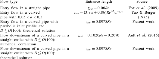
theoretical prediction. A summary of proposed development lengths for straight pipes, curved pipes and transitions is shown in table 3.
Summary of the development lengths related to straight pipes, curved pipes and transition. Transition lengths are given in number of pipe diameters.

4.2 Comparison with linearized theory
In § 3, we demonstrated how the dependence on
 $Re$
and
 $\unicode[STIX]{x1D6FC}$
can be eliminated from the equations governing the entry and exit flows in curved pipes. Here, we confirm the scalings (3.3) using numerical simulations. For
 $\unicode[STIX]{x1D6FC}=2.5\times 10^{-6}$
,
 $1.0\times 10^{-5}$
,
 $2.0\times 10^{-5}$
and
 $4.0\times 10^{-5}$
, and for
 $Re$
ranging from 30 to 200, corresponding to
 $2.3\times 10^{-3}<D<1.6$
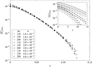
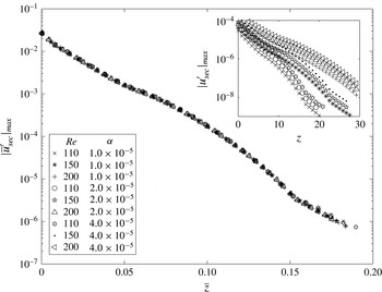
, the simulations confirm the scaling analysis of § 3. Figures 4–6 show the velocity and pressure fields for the developing flow in a curved pipe in both scaled and unscaled variables. The insets show the unscaled data. Axial cross-sections were taken along the pipe and the physical variables were determined on each cross-section. For example, figure 4 shows the maximum magnitude of the rescaled axial velocity
 $|\bar{u}_{z}^{\prime }|_{max}$
versus the rescaled axial coordinate
 $\bar{z}$
. Here, the axial velocity perturbation is rescaled by
 $Re^{2}\unicode[STIX]{x1D6FC}$
, and
 $z$
is rescaled by
 $Re$
, collapsing the data. Next, figure 5 shows the maximum magnitude of the rescaled secondary velocity
 $|\bar{u}_{sec}^{\prime }|_{max}$
, where
 $|\bar{u}_{sec}^{\prime }|^{2}=\bar{u}_{r}^{\prime 2}+\bar{u}_{\unicode[STIX]{x1D703}}^{\prime 2}$
. Since
 $u_{r}^{\prime }$
and
 $u_{\unicode[STIX]{x1D703}}^{\prime }$
scale with
 $Re\unicode[STIX]{x1D6FC}$
,
 $u_{sec}^{\prime }$
also scales with
 $Re\unicode[STIX]{x1D6FC}$
, and
 $z$
is again rescaled by
 $Re$
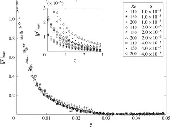
. Once again, the scalings collapse the numerical data. Finally, figure 6 shows the maximum magnitude of the rescaled pressure perturbation
 $|\bar{p}^{\prime }|_{max}$
, rescaled by
 $\unicode[STIX]{x1D6FC}$
, and
 $z$
is again scaled by
 $Re$
. We conclude by noting that the results in figures 4–6 include cases with
 $D=Re^{2}\unicode[STIX]{x1D6FC}=O(1)$
, and the scaling still holds, although (3.3) was strictly derived in the limit
 $D\ll 1$
.
Maximum magnitude of the numerically computed rescaled axial velocity component
 $\bar{u}_{z}^{\prime }$
for the developing flow in a curved pipe versus the rescaled axial coordinate
 $\bar{z}$
. Data points are shown for a range of
 $Re$
and
 $\unicode[STIX]{x1D6FC}$
. The inset shows the unscaled data. The data collapse when we apply the scalings of (3.3). Here, the Dean number is
 $0.1<D<1.6$
.

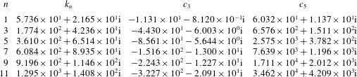
Eigenvalues
 $k_{n}$
of (3.22) along with
 $c_{3}$
and
 $c_{5}$
of the corresponding eigenfunctions
 $F_{n}(r)$
, assuming
 $c_{1}=1$
. These values can be used to generate the eigenfunctions seen in figure 2. It should be noted that
 $k_{n}$
,
 $c_{3}$
and
 $c_{5}$
for
 $n=2$
are complex conjugates of the corresponding values for
 $n=1$
. The
 $n=4,6,8,10,12$
values are likewise complex conjugates of the
 $n=3,5,7,9,11$
values respectively. Values are converged to four digits.

Maximum magnitude of the rescaled secondary velocity component
 $\bar{u}_{sec}^{\prime }$
for the developing flow in a curved pipe versus the rescaled axial coordinate
 $\bar{z}$
. Data points are shown for a range of
 $Re$
and
 $\unicode[STIX]{x1D6FC}$
. The inset shows the unscaled data. The data collapse when we apply the scalings of (3.3). Here, the Dean number is
 $0.1<D<1.6$
.

Maximum magnitude of the rescaled pressure perturbation
 $\bar{p}^{\prime }$
for the developing flow in a curved pipe versus the rescaled axial coordinate
 $\bar{z}$
. Data points are shown for a range of
 $Re$
and
 $\unicode[STIX]{x1D6FC}$
. The inset shows the unscaled data. The data collapse when we apply the scalings of (3.3). Here, the Dean number is
 $0.1<D<1.6$
.

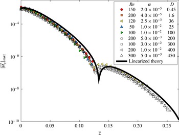
Finally, we compare the flow evolution from our numerical simulations for both the entry and exit problems with the linearized theoretical solution presented in § 3, i.e. equation (3.27). Figure 7 shows the numerically computed development of the axial velocity perturbation for a range of cases up to
 $D=O(100)$
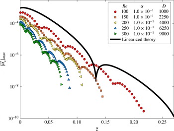
along with the theoretically predicted values from the solution given in (3.26). The results show a good agreement, suggesting that the linearized theory can reasonably capture the flow development in the curved pipe section for this range of Dean numbers. Figure 8 shows similar results, but for cases with
 $D>O(100)$
, demonstrating that the scaling arguments and linearized theory break down at sufficiently large Dean numbers. Based upon this comparison and the strong agreement between entrance lengths in figure 3, the linearized flow solution (3.26) can be expected to reasonably approximate the flow solution in the transition region both in the entry region of a curved pipe and downstream of a curved pipe in a straight outlet. It should be noted that each case in figures 7 and 8 shows the presence of axial spatial oscillations. The presence of these oscillations is clearly anticipated by the sine and cosine terms in (3.27).
Comparison of the rescaled numerical simulation results for both the entrance and exit problems with the linearized theory presented in § 3. The collapse shows that the linearized theory agrees well with the data up to
 $D=O(100)$
. Coloured symbols denote results for the developing curved pipe flow (entry problem) and open (white) symbols denote results for the flow downstream of a curved pipe (exit problem).

Comparison of the rescaled numerical simulation results for the entrance (developing) curved pipe flow problem with the linearized theory presented in § 3. The results show that the linearized theory breaks down above
 $D=O(100)$
.

5 Conclusion
We have identified scalings for the asymptotic velocity and pressure fields that can be used to eliminate all Reynolds number and curvature dependence from the continuity and linearized Navier–Stokes equations for the pressure-driven flow in the entry and exit regions of a curved pipe. These results were achieved by linearizing the Navier–Stokes equations in cylindrical coordinates about fully developed straight pipe Poiseuille flow and in toroidal coordinates about fully developed curved pipe Dean flow and applying judicious scalings (3.3), while considering the limits
 $D\ll 1$
and
 $Re\gg 1$
. We confirmed the scalings using three-dimensional Navier–Stokes simulations of both the entrance flow in a curved pipe and the exit flow downstream of a curved pipe into a straight outlet. As shown in figures 4–6, the results collapse when the scalings are applied. The governing equations and scalings have also been used to show that the transition lengths in both the entry and exit problems must be
 $O(dRe)$
, independent of
 $\unicode[STIX]{x1D6FC}$
; see (4.1). The prefactor depends on the type of inlet flow condition, i.e. uniform versus Dean flow.
Berger et al. (Reference Berger, Talbot and Yao1983) suggested that it might be possible to obtain an analytical solution for the low-Dean-number entry flow problem using a perturbation approach, although they appear never to have attempted such a solution. Here, we have developed such a solution using a separation of variables approach to simplify the governing equations (3.4) to an eigenvalue problem. Finally, we presented a numerical solution to this eigenvalue problem and showed that the achieved solution (3.26) agrees well with the results of full 3D numerical simulations up to a maximum Dean number of
 $D=O(100)$
.
As mentioned in § 3, we have applied Smith’s result (Smith Reference Smith1976) for
 $Re\gg 1$
that the upstream influence is negligible when solving the
 $O(dRe)$
entry problem in a curved pipe. We have extended this idea to the outlet problem and assumed that upstream influence is similarly negligible in the transition from a curved to a straight pipe, when looking at the
 $O(dRe)$
region downstream. This approach allowed us to apply Poiseuille flow as the inlet condition to the curved pipe for the entry problem, and Dean’s curved pipe velocity profile as the inlet condition to the straight pipe for the exit problem. The close fit between the theoretical prediction of this linearized theory and the 3D simulations (figure 7) further confirms Smith’s conclusion and supports our claim that upstream influence is similarly negligible for the exit problem.
We have demonstrated an equivalence between the entry and exit problems, such that by linearizing about their respective fully developed states, both problems can be written in terms of the same governing equations and boundary conditions (up to a factor of
 $-1$
). By the linearity of the equations, these ideas also show that the solution for developing curved pipe flow is a linear combination of the solution for flow downstream of a curved pipe and Dean’s analytical solution for fully developed flow in a curved pipe. Many questions remain to be addressed, especially for flows with larger Dean numbers and more severe curvature. For example, Smith & Duck (Reference Smith and Duck1980) identified flow structures and solution properties for plane channel flows subject to severe constriction, curves and corners. In general, these types of problems involve nonlinear partial differential equations and require numerical solutions, especially in more complex geometries. We have identified two cases (the entry and exit problems) in which analytical solutions can be found in the asymptotic limits
 $D\ll 1$
and
 $Re\gg 1$
, and numerically we have shown that these solutions are valid for
 $Re\geqslant 50$
and
 $D\leqslant 100$
. Based upon the theoretical approach used to obtain these results, it should be possible to develop a general solution for linearized pipe flow, providing a solution describing the decay of an arbitrary perturbation in a linearized pipe flow. This subject is left for a future article.
Acknowledgements
We thank K. Bulusu, V. Kulkarni and M. Plesniak of George Washington University for valuable discussions. K.K.C. was supported by the Viterbi Postdoctoral Fellowship through the Viterbi School of Engineering at the University of Southern California. We gratefully acknowledge the valuable suggestions of the reviewers.
Appendix A. Ordinary differential equation solution approach
In this appendix, we provide some details for the analysis presented in § 3.5. Analysing (3.22) and (3.23), we recognize that
 $F_{n}(r)$
is an odd function. We solve this eigenvalue problem by approximating the
 $F_{n}(r)$
as a Taylor series about
 $r=0$
, given by
 $$\begin{eqnarray}F_{n}(r)\approx c_{1}r+c_{3}r^{3}+c_{5}r^{5}+c_{7}r^{7}+\cdots \,,\end{eqnarray}$$
which automatically satisfies the conditions shown in (3.23). We fix
 $c_{1}=1$
to normalize the solutions. Here, the
 $n$
subscript on the coefficients
 $c_{i}$
has been dropped, but it is implicit that each eigenfunction
 $F_{n}(r)$
has a unique set of
 $c_{i}$
. Substitution of (A 1) into (3.22) yields recurrence relations for the
 $c_{i}$
, which are given by
 $$\begin{eqnarray}\displaystyle & \displaystyle c_{7}=k_{n}(2k_{n}c_{1}+(32-k_{n})c_{3}-24c_{5})/288, & \displaystyle\end{eqnarray}$$
 $$\begin{eqnarray}\displaystyle & \displaystyle c_{i}=\left(A_{i}c_{i-2}+B_{i}c_{i-4}+C_{i}c_{i-6}+D_{i}c_{i-8}\right)/E_{i}\quad \text{for}~i>7~\text{with}~i~\text{odd}, & \displaystyle\end{eqnarray}$$
 $$\begin{eqnarray}\displaystyle & \displaystyle A_{i}=4k_{n}(5-i)(i-3)^{2}(i-1), & \displaystyle\end{eqnarray}$$
 $$\begin{eqnarray}\displaystyle & \displaystyle B_{i}=4k_{n}[4(i-5)(i-3)-k_{n}](i-5)(i-3), & \displaystyle\end{eqnarray}$$
 $$\begin{eqnarray}\displaystyle & \displaystyle C_{i}=32k_{n}^{2}[23+(i-10)i], & \displaystyle\end{eqnarray}$$
 $$\begin{eqnarray}\displaystyle & \displaystyle D_{i}=-64k_{n}^{2}[31+(i-12)i], & \displaystyle\end{eqnarray}$$
 $$\begin{eqnarray}\displaystyle & \displaystyle E_{i}=(i-5)(i-3)^{2}(i-1)^{2}(i+1). & \displaystyle\end{eqnarray}$$
Each
 $c_{i}$
can be written in terms of
 $c_{3}$
,
 $c_{5}$
and
 $k_{n}$
(with
 $c_{1}=1$
), through recursive back-substitution. Extending this approach to high order, (A 1) can be written in terms only of
 $c_{3}$
,
 $c_{5}$
and
 $k_{n}$
. Substitution of this Taylor series into (3.24) at
 $r=1/2$
yields a set of three equations and three unknowns. In principle, this system can be solved to yield approximate values of the eigenvalues
 $k_{n}$
, and the associated values of
 $c_{3}$
and
 $c_{5}$
. The
 $F_{n}(r)$
are then given by (A 1), where each of the
 $c_{i}$
is uniquely determined by
 $c_{3}$
,
 $c_{5}$
and
 $k_{n}$
. In practice, this approach reduces to root-finding with a high-order polynomial in
 $k_{n}$
, the solutions of which can be achieved, for example, with a Newton iteration. With a modest number of terms, this approach provides reasonable guesses for the first few
 $k_{n}$
,
 $c_{3}$
and
 $c_{5}$
corresponding to the first few eigenfunctions.
To improve precision, the Taylor series should be used up to a small value of
 $r$
, and a shooting method should be used in the rest of the domain. This effectively handles the singular behaviour that is expected at
 $r=0$
when solving (3.22), and it also eliminates the need for a very-high-order Taylor series in order to obtain accuracy near
 $r=1/2$
. We use the Taylor series up to
 $r=0.1$
and use a fourth-order Runge–Kutta method elsewhere. We find that the results are not sensitive to this cutoff in the range [0.05, 0.3]. Finally, using the initial guesses for
 $c_{3}$
,
 $c_{5}$
and
 $k_{n}$
, a minimization scheme can be used to minimize the error in the boundary conditions (3.24). Using this approach, we have identified the first 12 eigenvalues
 $k_{n}$
and eigenfunctions
 $F_{n}(r)$
. The
 $k_{n}$
are given in table 4, along with the corresponding values of
 $c_{3}$
and
 $c_{5}$
. With
 $c_{1}=1$
and
 $c_{0}=c_{2}=c_{4}=\cdots =0$
, each
 $F_{n}(r)$
can be obtained from these values. Only the
 $k_{n}$
with positive real parts are retained to guarantee that the solution (3.21) decays to 0 as
 $\bar{z}\rightarrow \infty$
.
Appendix B. Numerical approach
Here, we describe the numerical methods used for the steady developing flow in a curved pipe, corresponding to the simulation domain shown in figure 1(b,c). For details on the simulations of the flow downstream of a curved pipe, see Ault et al. (Reference Ault, Chen and Stone2015). Here, the velocity vector
 $\boldsymbol{u}$
has been non-dimensionalized by
 $u_{avg}$
and lengths have been non-dimensionalized by
 $d$
. The incompressible Navier–Stokes equations were solved with a finite-volume solver adapted from the pimpleFoam solver of the OpenFOAM library (Weller et al. (Reference Weller, Tabor, Jasak and Fureby1998); additional details are provided in Ault et al.
Reference Ault, Chen and Stone2015). Spatial derivatives are second-order accurate, and the temporal scheme is fully implicit and second-order accurate. The average value of
 $|\unicode[STIX]{x1D735}\boldsymbol{\cdot }\boldsymbol{u}|<3\times 10^{-12}$
across all cells, and time steps are automatically adjusted to maintain a maximum Courant number of 0.5 in the mesh.
As a validation, we compare the computed fully developed velocity profiles in the curved pipe section,
 $\boldsymbol{u}_{FD}$
, with Dean’s analytical velocity profile,
 $\boldsymbol{u}_{D}$
. We quantify the error between the velocity profiles as
 $$\begin{eqnarray}\text{error}=\frac{\displaystyle \int _{\unicode[STIX]{x1D6FA}}\Vert \boldsymbol{u}_{FD}-\boldsymbol{u}_{D}\Vert \,\text{d}V}{\displaystyle \int _{\unicode[STIX]{x1D6FA}}\Vert \boldsymbol{u}_{D}\Vert \,\text{d}V},\end{eqnarray}$$
computed over the domain
 $\unicode[STIX]{x1D6FA}$
, where
 $\Vert \cdot \Vert$
is the L
 $^{2}$
norm. Typical values for our simulations have
 $\text{errors}\lesssim 10^{-3}$
, which should approach zero in the limits
 $\unicode[STIX]{x1D6FC}\ll 1$
and
 $D\ll 1$
, which are the appropriate limits for Dean’s solution. For our cases of interest, with
 $D\lesssim 1$
and
 $\unicode[STIX]{x1D6FC}\ll 1$
, errors are typically less than
 $10^{-3}$
, and Dean’s solution is valid to within 0.1 % for our flow conditions. A grid convergence study was performed for the highest
 $Re$
cases using grids with
 $7.5\times 10^{5}$
,
 $1.5\times 10^{6}$
,
 $3.0\times 10^{6}$
,
 $6.0\times 10^{6}$
and
 $1.2\times 10^{7}$
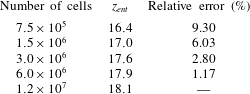
cells. Table 5 shows the entrance length,
 $z_{ent}$
, for the case
 $\unicode[STIX]{x1D6FC}=2.0\times 10^{-5}$
and
 $Re=200$
for each of the grids, where
 $z_{ent}$
represents the non-dimensional axial location where the axial velocity perturbation has reached 99 % of its final value. The table also lists relative percentage errors with respect to the finest grid. Steady-state solutions are achieved by running the solver until
 $$\begin{eqnarray}\left\Vert \frac{\unicode[STIX]{x2202}\boldsymbol{u}}{\unicode[STIX]{x2202}t}\right\Vert =\frac{1}{V}\int _{\unicode[STIX]{x1D6FA}}\left|\frac{\unicode[STIX]{x2202}\boldsymbol{u}}{\unicode[STIX]{x2202}t}\right|\,\text{d}V\end{eqnarray}$$
converges to
 $O(10^{-10})$
. A typical case requires approximately 5 h to run on 64 cores with
 $6.0\times 10^{6}$
cells.
Grid convergence results for developing curved pipe flow with
 $\unicode[STIX]{x1D6FC}=2.0\times 10^{-5}$
and
 $Re=200$
. Relative errors are with respect to the
 $1.2\times 10^{7}$
cell grid. Entrance lengths
 $z_{ent}$
have been non-dimensionalized by
 $d$
.

B.1 Boundary and initial conditions
At the inlet of the straight pipe (figure 1), we impose the parabolic velocity profile
 $\boldsymbol{u}=2\left(1-4r^{2}\right)\boldsymbol{e}_{z}$
(White Reference White2005), where
 $\boldsymbol{e}_{z}$
is the axial direction along the pipe and
 $r$
is the radial coordinate from the pipe centre. We also use the consistent pressure boundary condition (Gresho & Sani Reference Gresho and Sani1987) derived from the inlet-normal direction (
 $\boldsymbol{e}_{z}$
) of the Navier–Stokes equations, i.e.
 $$\begin{eqnarray}\boldsymbol{n}\boldsymbol{\cdot }\unicode[STIX]{x1D735}p=\boldsymbol{n}\boldsymbol{\cdot }\left(-\frac{\unicode[STIX]{x2202}\boldsymbol{u}}{\unicode[STIX]{x2202}t}-\unicode[STIX]{x1D735}\boldsymbol{\cdot }\left(\boldsymbol{u}\boldsymbol{u}\right)+\frac{1}{Re}\unicode[STIX]{x1D6FB}^{2}\boldsymbol{u}\right),\end{eqnarray}$$
which for our inlet condition reduces to
 $\unicode[STIX]{x2202}p/\unicode[STIX]{x2202}z=-32/Re$
. At the walls, we enforce the no-slip condition
 $\boldsymbol{u}=\mathbf{0}$
and the consistent pressure boundary condition (B 3) derived from the wall-normal direction of the Navier–Stokes equations. Finally, we set
 $\boldsymbol{n}\boldsymbol{\cdot }\unicode[STIX]{x1D735}\boldsymbol{u}=\mathbf{0}$
and
 $p=0$
at the outlet.