1 Introduction
The evolution of isolated patches of buoyant fluid may, perhaps, appear relatively straightforward, yet it turns out to be more complex than might at first be thought. Parcels of fluid that move and evolve relative to their environment under the action of a buoyancy force are often known as thermals, a name taken from the related atmospheric phenomenon exploited by birds and glider pilots (Scorer Reference Scorer1978) but also used to describe a wider range of buoyant phenomena.
The importance of these flows was recognised by Scorer (Reference Scorer1957) who performed a series of experiments to characterise turbulent thermals. The laminar analogue is somewhat less well studied however. An early description of the phenomenon can be found in On Growth and Form by D’Arcy Thompson (Thompson Reference Thompson1961) with the buoyant blob being the start of a ‘long story’ that is ‘deserving to be considered’. He describes the array of ‘beautiful vorticoid configurations’ as the phenomenon develops, noting its resemblance to the medusa or jellyfish. Griffiths (Reference Griffiths1986) investigated the development of thermals in high viscosity fluids, making observations of speed and velocity as the thermal developed. Sometimes the thermal formed a cap, and sometimes developed further into what he called a ‘toroidal chemical ring’. The existence of distinct stages of development is apparent from these observations, but a detailed examination of the different structures and clear explanations for their formation is not readily available.
Shlien & Thompson (Reference Shlien and Thompson1975) and Shlien (Reference Shlien1976) performed experiments with heat injection at a point, and observed the development of a thermal from a source that starts to accelerate, develops into a cap-like structure and then into a buoyant vortex ring. They note the key stages of development, but their experiments are limited in that they only observe the temperature field through shadowgraph data. Their discussion of the cap is limited, noting that the thermal transitions through this stage en route to forming a buoyant vortex ring. Their observations of the ring match well the theory of Turner (Reference Turner1957). Aside from these studies, the different stages in the life cycle of a laminar thermal are more frequently studied as separate phenomena in their own right. To the best of our knowledge, no-one has yet treated the blob, cap and ring as different stages of the same process and tried to link their development.
Davidson, Sreenivasan & Aspden (Reference Davidson, Sreenivasan and Aspden2007) present a model for a mushroom-like cap that develops from a buoyant disturbance. They make predictions about how the structure and velocities of the cap will develop, but without any comparison to experiments or simulations. As a result they do not make any observations about how the cap develops into a ring, and note an apparent paradox in their model in that the cap velocity tends towards a constant value whilst the total impulse of the fluid continues to grow linearly in time.
Gharib, Rambod & Shariff (Reference Gharib, Rambod and Shariff1998) performed experiments on non-buoyant vortex rings generated using an impulsive piston. They find evidence for the existence of a universal time scale for the pinch off of the vortex ring from the trailing wake. At long times, the vorticity flux of the ring is constant and equal to that of the entire domain at an earlier time
 $t$
. When
 $t$
is made into a dimensionless property
 $t^{\ast }$
it is found to be independent of the strength of the impulse generated by the piston. This is rationalised by arguing that a stable vortex ring represents a maximum in energy subject to a given impulse and vorticity flux. As a result, a critical non-dimensional energy can be calculated for the vortex ring. Once the developing flow from the piston drops below this critical value the ring pinches off from the developing wake to move away as a stable vortex ring.
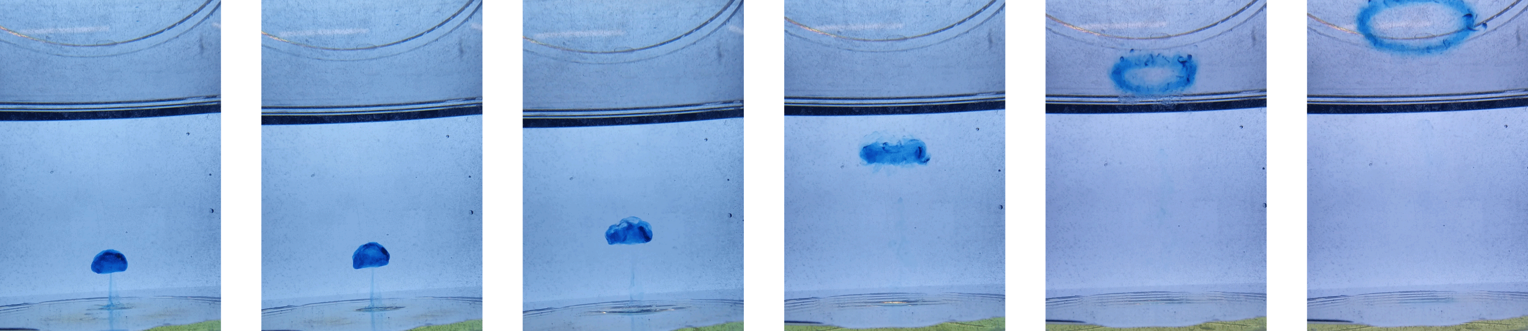
We have performed numerical simulations of laminar thermals and observed an interesting life cycle in which a buoyant perturbation develops, via an initial transient, into a mushroom-like cap structure and then into a buoyant vortex ring. This behaviour is illustrated in figure 1 which shows an experiment conducted as part of this study. The experiment is similar to that of Sànchez et al. (Reference Sànchez, Raymond, Libersky and Petschek1989), where a dyed buoyant thermal is released into fresh water. Following release, the thermal has developed into a mushroom cap with a wake which subsequently detaches. The cap then wraps up into a vortex ring.
Laboratory observations of a laminar thermal.

The primary purpose of this study is to characterise the entire life cycle of a laminar thermal, from its initiation and development into a mushroom-like cap through to the separation of a buoyant vortex ring at the front and the development of the resulting wake. One surprising finding is that the wake can itself roll up to form a secondary vortex ring.
2 Governing equations
Consider an axisymmetric, incompressible, Boussinesq fluid with mean density
 $\bar{\unicode[STIX]{x1D70C}}$
and a density perturbation of
 $\unicode[STIX]{x1D6FF}\unicode[STIX]{x1D70C}$
. We can write this density perturbation in terms of a temperature field,
 $T$
, as
 $\unicode[STIX]{x1D6FF}\unicode[STIX]{x1D70C}=-\bar{\unicode[STIX]{x1D70C}}\unicode[STIX]{x1D6FD}T$
, where
 $T$
is the perturbation from a background temperature
 $T_{0}$
, and
 $\unicode[STIX]{x1D6FD}$
a thermal expansion coefficient. The governing equations for this system in terms of velocity
 $\boldsymbol{u}$
and pressure
 $p$
are,
 $$\begin{eqnarray}\frac{\text{D}\boldsymbol{u}}{\text{D}t}=-\unicode[STIX]{x1D735}\left(\frac{p}{\bar{\unicode[STIX]{x1D70C}}}\right)-\boldsymbol{g}\unicode[STIX]{x1D6FD}T+\unicode[STIX]{x1D708}\unicode[STIX]{x1D6FB}^{2}\boldsymbol{u},\end{eqnarray}$$
and
 $$\begin{eqnarray}\frac{\text{D}T}{\text{D}t}=\unicode[STIX]{x1D6FC}\unicode[STIX]{x1D6FB}^{2}T,\end{eqnarray}$$
where
 $\boldsymbol{g}$
is the acceleration due to gravity,
 $\unicode[STIX]{x1D708}$
and
 $\unicode[STIX]{x1D6FC}$
are, respectively, the kinematic viscosity and thermal diffusivity, both assumed independent of temperature, and the hydrostatic pressure has been absorbed into the pressure term.
The corresponding equation for azimuthal vorticity
 $\unicode[STIX]{x1D714}_{\unicode[STIX]{x1D703}}$
is, in cylindrical polar coordinates
 $(r,\unicode[STIX]{x1D703},z)$
,
 $$\begin{eqnarray}\frac{\text{D}}{\text{D}t}\left(\frac{\unicode[STIX]{x1D714}_{\unicode[STIX]{x1D703}}}{r}\right)=-\frac{g\unicode[STIX]{x1D6FD}}{r}\frac{\unicode[STIX]{x2202}T}{\unicode[STIX]{x2202}r}+\unicode[STIX]{x1D708}\frac{1}{r^{2}}\unicode[STIX]{x1D6FB}_{\ast }^{2}\left(r\unicode[STIX]{x1D714}_{\unicode[STIX]{x1D703}}\right),\end{eqnarray}$$
where
 $$\begin{eqnarray}\unicode[STIX]{x1D6FB}_{\ast }^{2}=r\frac{\unicode[STIX]{x2202}}{\unicode[STIX]{x2202}r}\left(\frac{1}{r}\frac{\unicode[STIX]{x2202}}{\unicode[STIX]{x2202}r}\right)+\frac{\unicode[STIX]{x2202}^{2}}{\unicode[STIX]{x2202}z^{2}}\end{eqnarray}$$
is the Stokes operator. Note that (2.3) may be re-written as
 $$\begin{eqnarray}\frac{\text{D}}{\text{D}t}\left(\frac{1}{2}r\unicode[STIX]{x1D714}_{\unicode[STIX]{x1D703}}\right)=g\unicode[STIX]{x1D6FD}T+\unicode[STIX]{x1D735}\boldsymbol{\cdot }\boldsymbol{F}+\frac{1}{2}\unicode[STIX]{x1D708}\unicode[STIX]{x1D6FB}_{\ast }^{2}(r\unicode[STIX]{x1D714}_{\unicode[STIX]{x1D703}}),\end{eqnarray}$$
where the flux
 $\boldsymbol{F}$
is
 $$\begin{eqnarray}\boldsymbol{F}={\textstyle \frac{1}{2}}(u_{r}^{2}-u_{z}^{2})\hat{\boldsymbol{e}}_{z}-u_{r}u_{z}\hat{\boldsymbol{e}}_{r}-{\textstyle \frac{1}{2}}g\unicode[STIX]{x1D6FD}Tr\,\hat{\boldsymbol{e}}_{r},\end{eqnarray}$$
 $\hat{\boldsymbol{e}}$
being a unit vector in a coordinate direction.
It follows from (2.3) and (2.5) that, for a localised disturbance (see Davidson et al. Reference Davidson, Sreenivasan and Aspden2007),
 $$\begin{eqnarray}\displaystyle & \displaystyle \frac{\text{d}}{\text{d}t}\int _{V_{\infty }}\left(\frac{\unicode[STIX]{x1D714}_{\unicode[STIX]{x1D703}}}{r}\right)\,\text{d}V=2\unicode[STIX]{x03C0}g\unicode[STIX]{x1D6FD}\int _{-\infty }^{\infty }T_{r=0}\,\text{d}z+4\unicode[STIX]{x03C0}\unicode[STIX]{x1D708}\int _{-\infty }^{\infty }\left(\frac{\unicode[STIX]{x1D714}_{\unicode[STIX]{x1D703}}}{r}\right)_{r=0}\,\text{d}z, & \displaystyle\end{eqnarray}$$
 $$\begin{eqnarray}\displaystyle & \displaystyle \frac{\text{d}}{\text{d}t}\int _{V_{\infty }}\frac{1}{2}r\unicode[STIX]{x1D714}_{\unicode[STIX]{x1D703}}\,\text{d}V=\int _{V_{\infty }}g\unicode[STIX]{x1D6FD}T\,\text{d}V, & \displaystyle\end{eqnarray}$$
for an infinite domain,
 $V_{\infty }$
, with the fluid at rest and
 $T=0$
in the far field. Note that the buoyant growth of the integral of
 $\unicode[STIX]{x1D714}_{\unicode[STIX]{x1D703}}/r$
in (2.7) depends only on the centreline temperature. These two equations can then be related to more familiar properties of the flow as follows:
 $$\begin{eqnarray}\unicode[STIX]{x1D6F7}=\frac{1}{2\unicode[STIX]{x03C0}}\int _{V_{\infty }}\frac{\unicode[STIX]{x1D714}_{\unicode[STIX]{x1D703}}}{r}\,\text{d}V,\end{eqnarray}$$
where
 $\unicode[STIX]{x1D6F7}$
is the flux of azimuthal vorticity (or circulation) in the axisymmetric system, and
 $$\begin{eqnarray}\boldsymbol{L}=\int _{V_{\infty }}{\textstyle \frac{1}{2}}r\unicode[STIX]{x1D714}_{\unicode[STIX]{x1D703}}\,\text{d}V\,\hat{\boldsymbol{e}}_{z}={\textstyle \frac{1}{2}}\int _{V_{\infty }}\left(\boldsymbol{x}\times \unicode[STIX]{x1D74E}\right)\,\text{d}V,\end{eqnarray}$$
where the integral on the right is the net linear impulse of the fluid in an infinite domain (
 $\boldsymbol{x}$
being a position vector). The property
 $\boldsymbol{L}$
can be related to the net linear momentum according to
 $\boldsymbol{L}=\int \boldsymbol{u}\,\text{d}V$
(Saffman Reference Saffman1992). Note that, since (2.2) requires
 $\int T\,\text{d}V=$
constant, equation (2.8) implies a linear growth in
 $\boldsymbol{L}$
,
 $$\begin{eqnarray}|\boldsymbol{L}|=t\int _{V_{\infty }}g\unicode[STIX]{x1D6FD}T\,\text{d}V.\end{eqnarray}$$
Note also that, when the viscous term is weak in (2.7), it is well approximated by
 $$\begin{eqnarray}\frac{\text{d}\unicode[STIX]{x1D6F7}}{\text{d}t}=g\unicode[STIX]{x1D6FD}\int _{-\infty }^{\infty }T_{r=0}\,\text{d}z.\end{eqnarray}$$
Dimensional analysis can be performed by introducing some characteristic length scale and temperature for the thermal, say
 $l$
and
 $\hat{T}$
respectively, based on the initial condition as discussed below (3.1). There are two dimensionless groups that define the problem, a Reynolds number
 $Re$
, and a Prandtl number
 $Pr$
,
 $$\begin{eqnarray}Re=\frac{Ul}{\unicode[STIX]{x1D708}},\quad Pr=\frac{\unicode[STIX]{x1D708}}{\unicode[STIX]{x1D6FC}},\end{eqnarray}$$
where
 $U$
is the velocity scale
 $$\begin{eqnarray}U=\sqrt{g\unicode[STIX]{x1D6FD}\hat{T}l}.\end{eqnarray}$$
In addition to these dimensionless groups, a characteristic time scale, impulse, and vorticity flux for the problem can be defined as,
 $$\begin{eqnarray}t_{0}=\frac{l}{U},\quad L_{0}=Ul^{3},\quad \unicode[STIX]{x1D6F7}_{0}=Ul.\end{eqnarray}$$
We shall use these to non-dimensionalise quantities, with
 $\unicode[STIX]{x1D70F}=t/t_{0}$
being dimensionless time.
We also introduce the non-dimensional variable,
 $$\begin{eqnarray}\unicode[STIX]{x1D6FE}=\frac{l^{2}\unicode[STIX]{x1D6F7}}{|\boldsymbol{L}|},\end{eqnarray}$$
as a diagnostic for the flow. Mathematically this is a dimensionless ratio of the zeroth and second moments of the vorticity field. It tells us about the relative compactness of the vorticity distribution around the axis; the more spread out the vorticity is, the smaller the value of
 $\unicode[STIX]{x1D6FE}$
.
3 Numerical simulations
Numerical simulations were performed using an axisymmetric finite difference method. The equations of motion are solved using second-order spatial differences and first-order integration in time from some specified initial condition. The fluid is viscous and Boussinesq, and the boundary conditions on the domain are no slip and adiabatic. The domain is large (radius of
 $R=14\,l$
, height of
 $H=80\,l$
) relative to the size of the thermal. The numerical methods are based on those of Harlow & Welch (Reference Harlow and Welch1965), adapted for an axisymmetric coordinate system and to include buoyancy. Simulations were performed using a staggered mesh of 4000 axial
 $\times$
350 radial cells with finer resolution near the axis than at the edges. Spatial and temporal resolution studies were performed by increasing and decreasing both the mesh resolution and timestep and ensuring that the results were converged.
We use the same initial condition as Davidson et al. (Reference Davidson, Sreenivasan and Aspden2007) with
 $\boldsymbol{u}=0$
and a Gaussian temperature perturbation of the form
 $$\begin{eqnarray}T=\hat{T}\exp \left(-\frac{r^{2}+z^{2}}{l^{2}}\right)\end{eqnarray}$$
in an ambient background
 $T=0$
. The location of the Gaussian blob is
 $r=0$
and
 $z=H/10$
above the bottom of the domain.
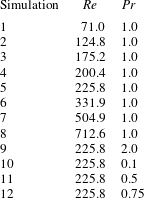
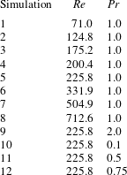
A range of cases for different
 $Re$
and
 $Pr$
were examined, details of which are given in table 1. They cover a range of Reynolds numbers, with the Prandtl number being fixed at 1.0, but also include some variation in Prandtl number for
 $Re=225.8$
.
Details of simulations.
4 The life cycle and evolution process
As discussed, the laminar thermal passes through a number of phases during its life cycle. These can be summarised as the buoyant blob, the mushroom-like cap and the buoyant vortex ring, each of which will be discussed in detail in subsequent sections. To illustrate these stages we take a typical simulation at
 $Re=225.8$
and
 $Pr=1$
. As we shall see, for this simulation a blob is maintained in the time range
 $\unicode[STIX]{x1D70F}=0$
–2.5, the cap for approximately
 $\unicode[STIX]{x1D70F}=7$
–17, and the ring from
 $\unicode[STIX]{x1D70F}=23$
onwards.
4.1 An overview of the life cycle and evolution
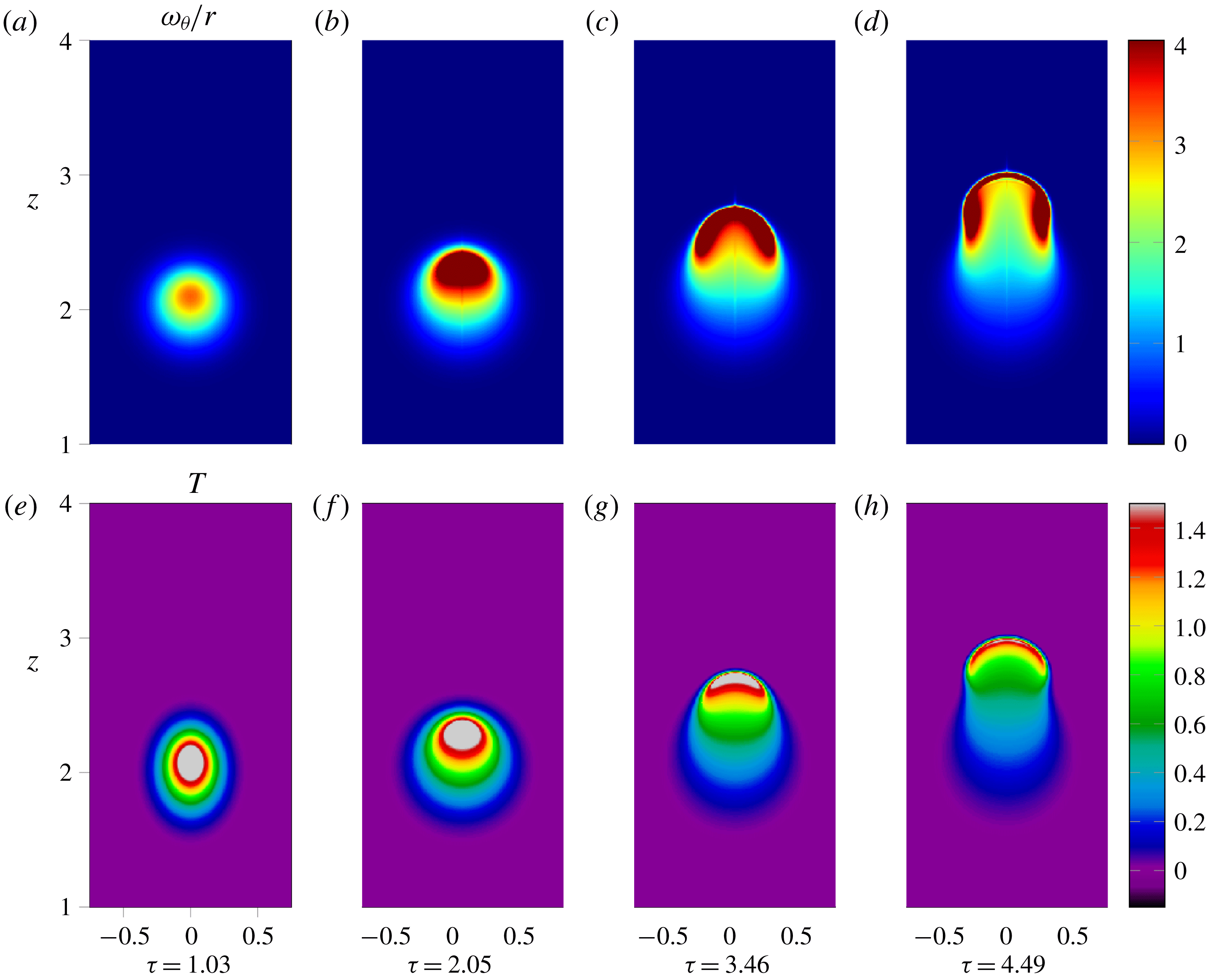
Early stages in the development of a thermal. Contours of
 $\unicode[STIX]{x1D714}_{\unicode[STIX]{x1D703}}/r$
(a–d) and temperature (e–h) at different dimensionless times
 $\unicode[STIX]{x1D70F}$
.

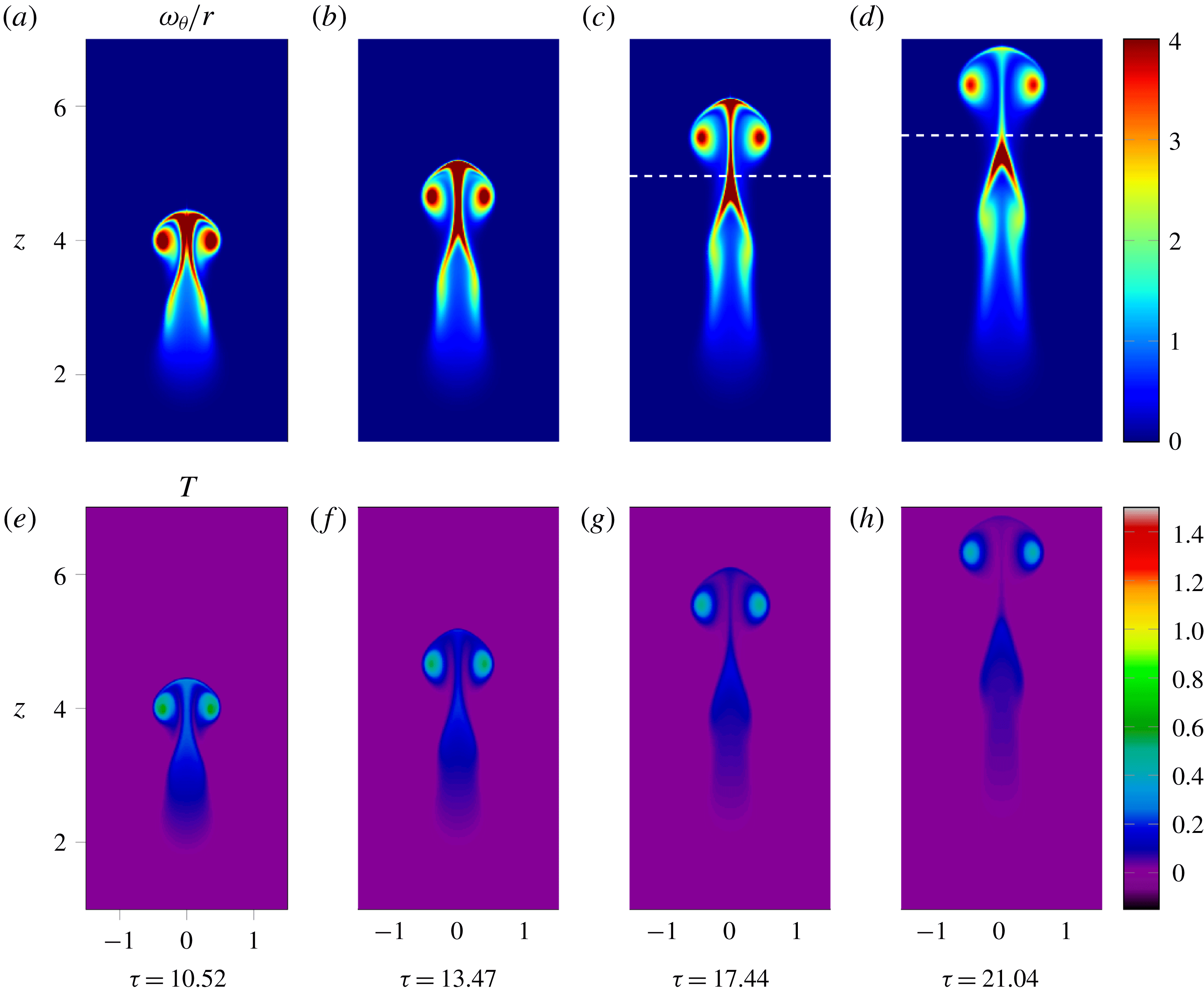
There are a number of key events in the life cycle that characterise each of the stages, and the transitions between them. These are illustrated below, and can be described as follows. First, vorticity is generated by radial temperature gradients. This results in a Gaussian distribution of
 $\unicode[STIX]{x1D714}_{\unicode[STIX]{x1D703}}/r$
developing immediately following initiation, as can be seen in figure 2(a). This Gaussian distribution is relatively short lived, however, as the blob begins to lift under the action of buoyancy forces. The effect of this is greatest at the centre of the buoyant blob, as can be seen in figure 2(b). The temperature field is advected with the fluid, as is
 $\unicode[STIX]{x1D714}_{\unicode[STIX]{x1D703}}/r$
, although
 $\unicode[STIX]{x1D714}_{\unicode[STIX]{x1D703}}/r$
continues to be generated by radial temperature gradients.
As the blob continues to lift, it enters a stage of significant distortion, with cooler fluid being swept in from the rear. The faster moving fluid near the axis advects the temperature and
 $\unicode[STIX]{x1D714}_{\unicode[STIX]{x1D703}}/r$
upward into a rapidly thinning front at the leading edge of the blob. This can be seen in figures 2(c) and 2(d) from
 $\unicode[STIX]{x1D70F}=3.5$
–4.5. In addition to this thinning front, the higher temperature fluid is also displaced radially outwards into a cylindrical annulus, carrying with it vorticity. This is illustrated in figure 2(d), and marks the end of the buoyant blob and transition towards the mushroom cap.
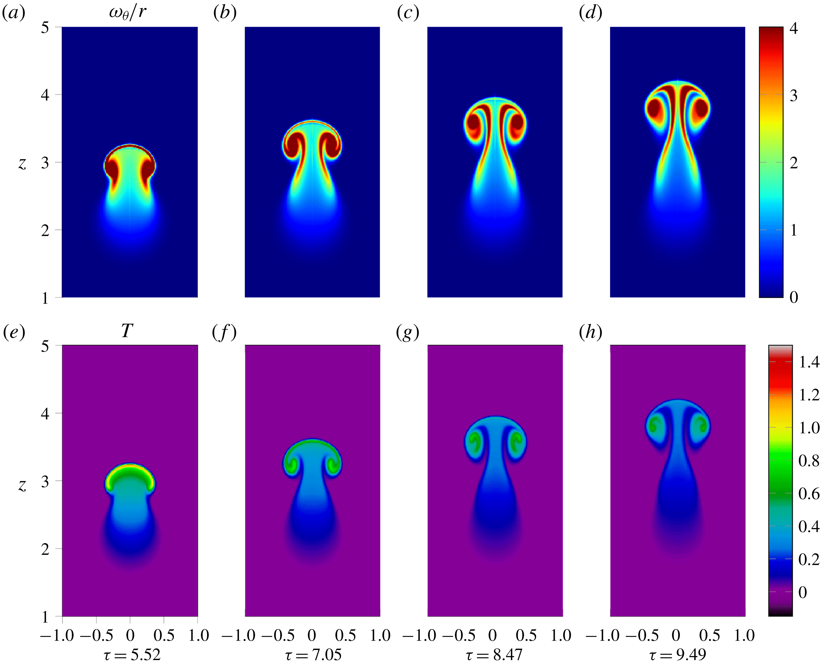
This transition from blob to mushroom-like cap is characterised by the roll-up at the sides of the thermal taking place from
 $\unicode[STIX]{x1D70F}=4.5$
–7.0. The vorticity that has been displaced radially outwards in a concentrated annulus below the front induces a rotational motion and begins to wrap up on itself, as shown in figure 3(a), to form the lobes that will eventually become the buoyant vortex ring. The induced motion of this vorticity field sweeps fluid upwards at the centre of the thermal and radially outwards at the front, causing the front to thin at an ever increasing rate as predicted by Davidson et al. (Reference Davidson, Sreenivasan and Aspden2007).
Intermediate stages in the development of a thermal. Contours of
 $\unicode[STIX]{x1D714}_{\unicode[STIX]{x1D703}}/r$
(a–d) and temperature (e–h) at different times
 $\unicode[STIX]{x1D70F}$
.

The mushroom cap is established by figure 3(b),
 $\unicode[STIX]{x1D70F}=7.0$
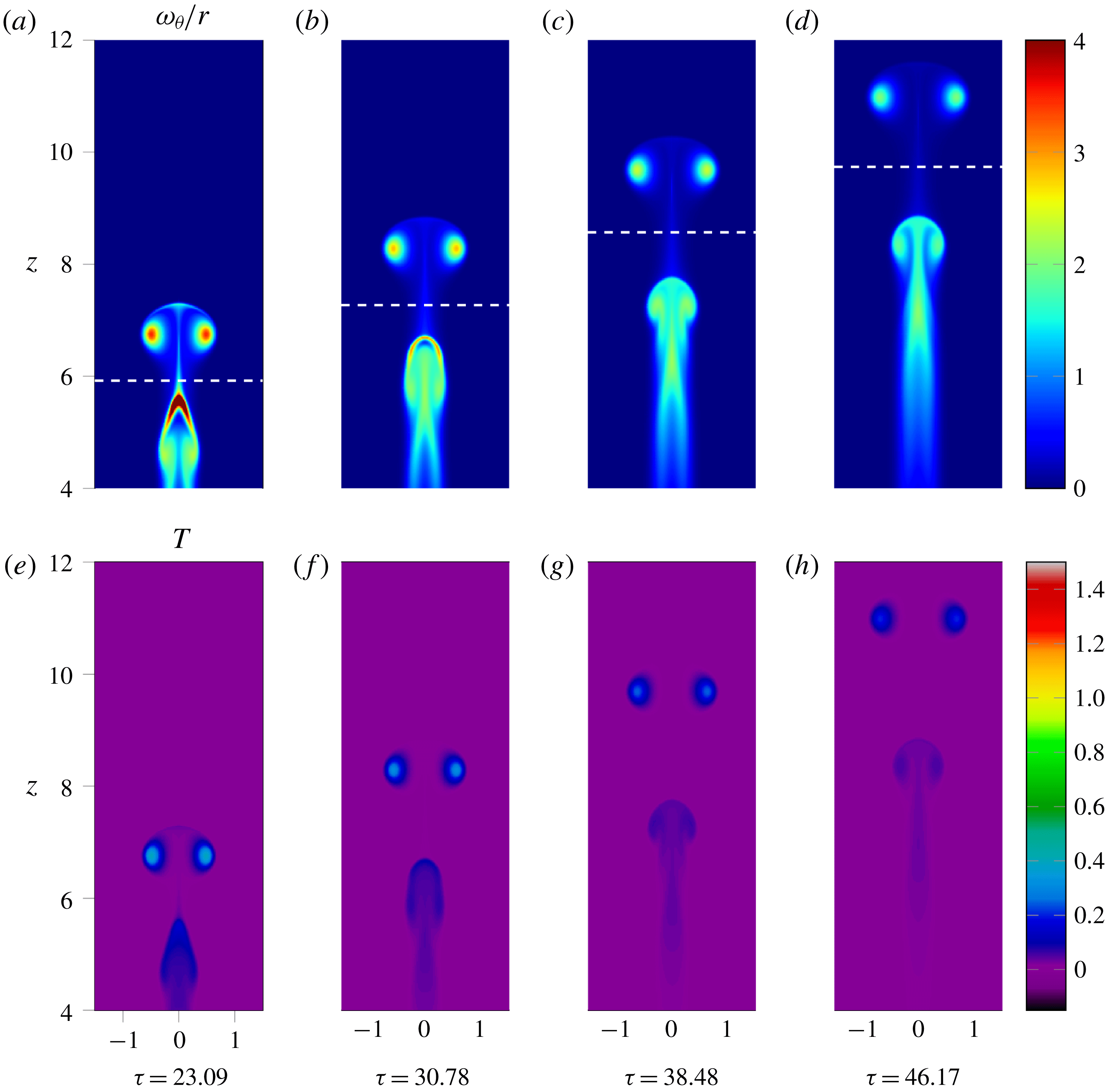
. The thermal continues to entrain fluid at the rear, increasing its volume and stretching the front further to a point at which it pinches apart at the axis. As can be seen by comparing the upper images of figures 3(b) and 3(c), this occurs between
 $\unicode[STIX]{x1D70F}=7.0$
and
 $\unicode[STIX]{x1D70F}=8.5$
, with further investigation showing it to be around
 $\unicode[STIX]{x1D70F}=8.0$
. This is the first of several morphological changes. It can be seen in figure 3(c) that once punctured this thin front is rapidly swept up into the lobes of vorticity. Below the mushroom cap a warm wake forms where the thermal has passed through. Though cooler than the cap, high radial gradients in temperature define a sharp edge to this region generating new vorticity that forms trailing tendrils below the cap. These can be seen developing in figures 3(c) and 3(d).
Later stages in the development of a thermal. Contours of
 $\unicode[STIX]{x1D714}_{\unicode[STIX]{x1D703}}/r$
(a–d) and temperature (e–h) at different dimensionless times
 $\unicode[STIX]{x1D70F}$
.

Up until the formation of the cap, the thermal has been accelerating from its starting position as we will show shortly. Once the mushroom cap has been achieved, however, the acceleration falls and the cap tends towards a constant velocity,
 $u$
, as predicted by Davidson et al. (Reference Davidson, Sreenivasan and Aspden2007). Fluid continues to be entrained at the base of the cap as the vorticity in the lobes induces a flow radially inwards and up along the axis. As a result of this motion the trailing tendrils of vorticity are swept inwards towards the axis and stretched vertically resulting in necking that can be seen developing in figure 4(b). Eventually this reaches a point where the stem of vorticity connecting the cap to the wake becomes sufficiently weak, as illustrated in figure 4(d), that we can consider two distinct regions of flow; the buoyant vortex ring and the wake. This transition process is illustrated in figures 4(b–d) and marks the second morphological change. The upper part of the stem, which is connected to the cap, is swept upwards and out along the front of the cap to eventually become wrapped up in the buoyant vortex ring. As a result, the cap shape is preserved until around
 $\unicode[STIX]{x1D70F}=17.0$
. Beyond this point the vast majority of the vorticity has been swept up in the ring and it can now be regarded as a separate region of flow moving off ahead of the wake. The lower portion of the trailing vorticity stem is subsumed by the wake, and begins to display qualitative similarities to the developing thermal of figure 2(d). Indeed, we find that after a period of time the wake can evolve in a similar way to the initial thermal and produce a second mushroom-like cap that separates in the same way to form a secondary vortex ring. The early stages of this behaviour can be seen in figure 5 and will be discussed in § 4.5.
Late stages in the development of a thermal showing a second cap and ring beginning to form. Contours of
 $\unicode[STIX]{x1D714}_{\unicode[STIX]{x1D703}}/r$
(a–d) and temperature (e–h) at different dimensionless times
 $\unicode[STIX]{x1D70F}$
.

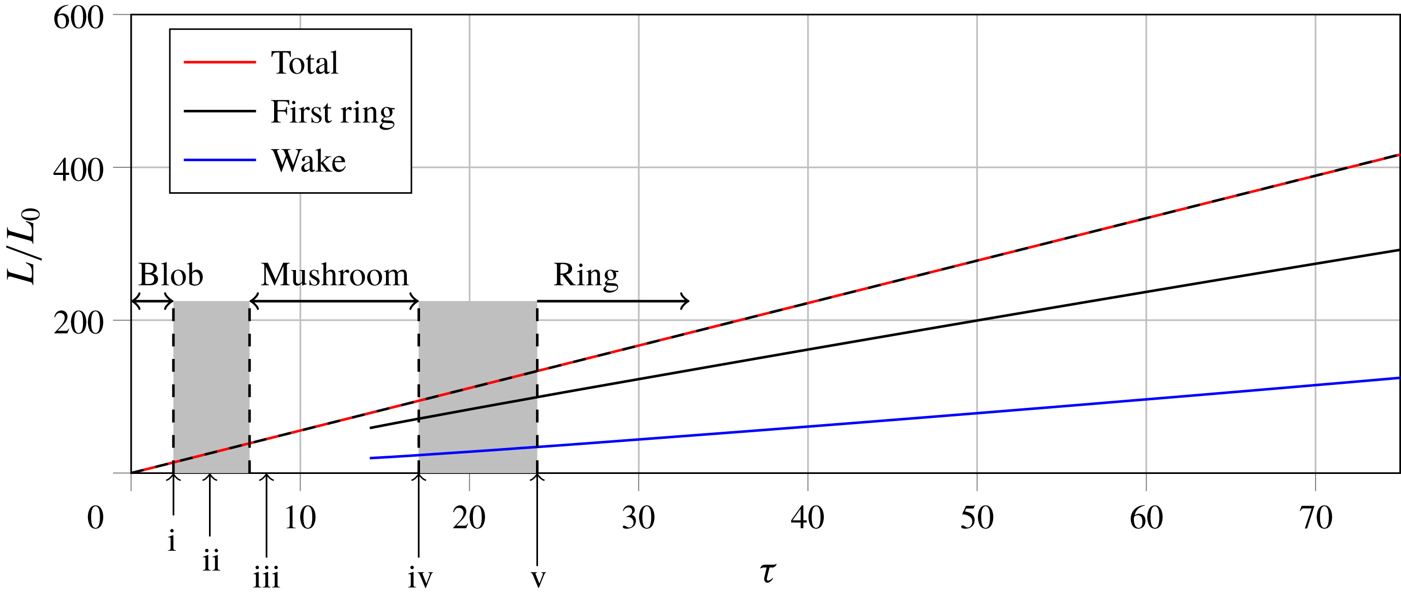
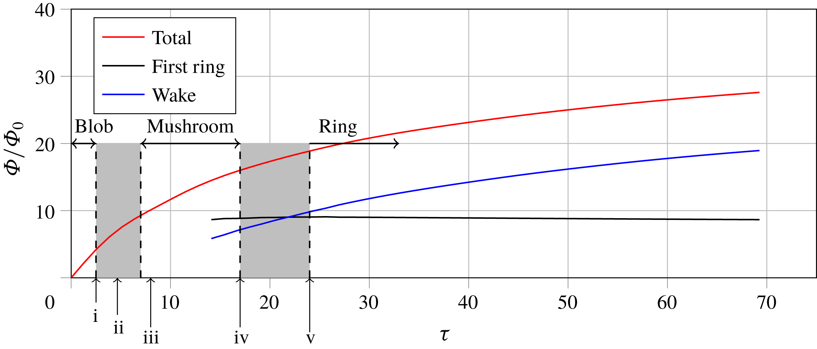
There are a number of quantities of interest that can be observed over the course of this cycle. Plotted in figures 6 and 7 are the impulse
 $L$
and flux
 $\unicode[STIX]{x1D6F7}$
for the entire flow, and also individually for the ring and wake. This was achieved by splitting the domain into two regions, with the mushroom cap or ring contained within the upper one and the wake below. This is indicated in figures 4 and 5 by the white dashed lines. (The white lines indicate the minimum in
 $\int \unicode[STIX]{x1D714}_{\unicode[STIX]{x1D703}}\,\text{d}r$
as a function of
 $z$
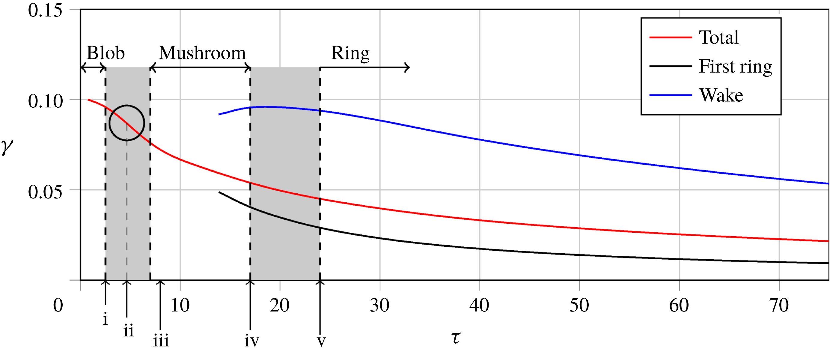
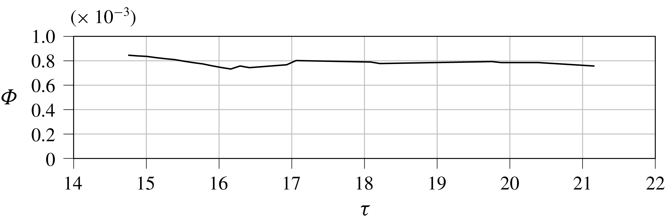
as a way of distinguishing the two parts.) It can be seen from figure 6 that the impulse for the overall flow increases linearly in time, consistent with (2.11), as does the impulse of both the cap-come-ring and the wake. Figure 7 shows that the vorticity flux of the overall flow increases monotonically, but the rate of increase slows as hotter fluid is swept away from the axis. This is consistent with (2.12). The flux of the cap attains a constant value as the buoyant ring is formed. The dimensionless parameter
 $\unicode[STIX]{x1D6FE}$
can be calculated and is plotted in figure 8. It can be seen that
 $\unicode[STIX]{x1D6FE}$
for the entire flow initially begins to fall at an increasing rate as the blob accelerates before starting to level off as the cap and ring form. Once formed,
 $\unicode[STIX]{x1D6FE}$
of the cap/ring decreases as
 $\unicode[STIX]{x1D70F}^{-1}$
, reflecting the linear growth in
 $L$
.
 $\unicode[STIX]{x1D6FE}$
of the wake initially rises, reaching a maximum as the wake begins to roll up into a second cap around
 $\unicode[STIX]{x1D70F}=18$
, beyond which point it too falls monotonically.
Evolution of impulse for the thermal, the first ring, and the wake. The grey regions denote transition between stages whilst i–iv denote key points in the life cycle as discussed in the text. These are: i the end of constant acceleration and the blob phase, discussed in § 4.2; ii the inflexion point in
 $\unicode[STIX]{x1D6FE}$
and beginning of roll up, discussed in § 4.2; iii the pinching apart of the cap front, discussed in § 4.3; iv the point at which the ring core becomes stronger than the stem, discussed in § 4.3; v the separation of the buoyant ring and wake by necking, discussed in § 4.4.2. Note that iii occurs shortly after the beginning of the mushroom cap phase discussed in § 4.3. The dashed black line is the total impulse predicted by (2.11).

Evolution of flux for the thermal, the first ring and the wake. Points i–v as for figure 6.

Evolution of
 $\unicode[STIX]{x1D6FE}$
for the thermal, the first ring and the wake. Points i–v as for figure 6 with the inflexion point (ii) circled.

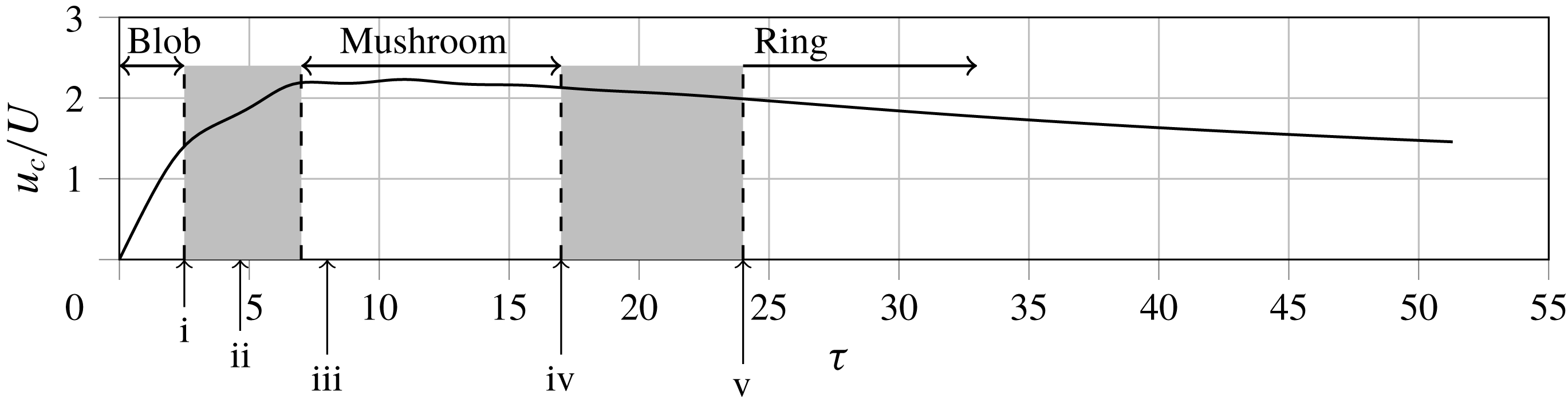
Figure 9 shows the maximum dimensionless vertical velocity on the axis. It can be seen that the blob initially undergoes a period of constant acceleration until around
 $\unicode[STIX]{x1D70F}=2.5$
. After this the acceleration decreases, with the velocity attaining an approximately constant value from
 $\unicode[STIX]{x1D70F}=7.0$
–15.0. This coincides with the mushroom cap phase of the thermal, as predicted by Davidson et al. (Reference Davidson, Sreenivasan and Aspden2007). Beyond this the velocity begins to fall as the thermal transitions into a buoyant vortex ring.
Maximum dimensionless vertical velocity on the
 $z$
-axis against
 $\unicode[STIX]{x1D70F}$
. Points i–v as for figure 6.

We will now discuss in more detail the different stages of the flow explaining the observations above and examining the transitions between each stage.
4.2 Stage 1: the buoyant blob
The first stage in the development of the thermal is take-off of the initial temperature perturbation and compression into a front. Starting with undisturbed fluid, we initially have zero vorticity,
 $\unicode[STIX]{x1D714}_{\unicode[STIX]{x1D703}}$
, and no motion. The very first stage, therefore, is vorticity generation by radial temperature gradients (figure 2
a). Following this, the hottest fluid in the centre of the thermal begins to rise fastest under the action of buoyancy, and the
 $\unicode[STIX]{x1D714}_{\unicode[STIX]{x1D703}}/r$
and
 $T$
fields are compressed into rapidly thinning fronts (figures 2
b and 2
c).
It can be seen from figure 9 that the thermal initially undergoes a period of approximately constant acceleration. This was observed experimentally by Shlien (Reference Shlien1976) who state that they could offer no simple interpretation for the behaviour. It can be understood, however, by considering the terms in (2.1). At
 $\unicode[STIX]{x1D70F}=0$
there is no fluid motion, and
 $\boldsymbol{u}$
remains small for some time. Initially, therefore, there must be a balance between
 $\unicode[STIX]{x2202}\boldsymbol{u}/\unicode[STIX]{x2202}t$
and
 $-\boldsymbol{g}\unicode[STIX]{x1D6FD}T$
. Since, in the absence of significant motion,
 $T$
evolves only slowly through diffusion, the vertical velocity must increase approximately linearly in time, i.e. constant acceleration. The neglect of
 $\boldsymbol{u}\boldsymbol{\cdot }\unicode[STIX]{x1D735}\boldsymbol{u}$
by comparison with
 $\unicode[STIX]{x2202}\boldsymbol{u}/\unicode[STIX]{x2202}t$
is valid for times such that
 $t\ll l/U$
, and the requirement that the diffusion of
 $T$
is small during this period is satisfied provided that
 $Ul/\unicode[STIX]{x1D6FC}\gg 1$
(see appendix A). As the velocity increases however, the balance of terms in (2.1) changes with the buoyancy now increasingly being balanced by
 $\boldsymbol{u}\boldsymbol{\cdot }\unicode[STIX]{x1D735}\boldsymbol{u}$
. As a result the acceleration begins to fall, and the front of the thermal approaches a steady velocity, as discussed by Davidson et al. (Reference Davidson, Sreenivasan and Aspden2007). The end of the period of roughly constant acceleration marks the end of the buoyant blob phase, with the change in force balance and approach to constant maximum velocity marking the transition from blob to mushroom cap.
Looking at the plot of
 $\unicode[STIX]{x1D6FE}$
for the entire flow (figure 8), there is an inflexion point around
 $\unicode[STIX]{x1D70F}=4.5$
accompanied by a morphological change as the lobes of the thermal begin to roll up. To understand this, note that
 $\unicode[STIX]{x1D6F7}$
increases monotonically according to (2.12) as the temperature front thins along the axis. At short times this growth in
 $\unicode[STIX]{x1D6F7}$
is linear, but as hot fluid is radially displaced the source term decreases, so the value of
 $\unicode[STIX]{x1D6F7}$
increases at an ever slowing rate. Since impulse increases linearly in time, as discussed above, an inflexion point becomes inevitable, with
 $\unicode[STIX]{x1D6FE}$
transitioning from
 $\unicode[STIX]{x1D6FE}\sim \unicode[STIX]{x1D70F}^{0}$
to
 $\unicode[STIX]{x1D6FE}\sim \unicode[STIX]{x1D70F}^{-1}$
. This coincides with the transition into the mushroom cap phase.
4.3 Stage 2: the mushroom cap
As a front forms at the leading edge of the thermal, fluid is displaced to the sides (figure 2
d) and vorticity collects in a torus, covered by a thin cap or front (figure 3
b). There are trailing tendrils of vorticity to the rear that form due to the sharp radial temperature gradients at the edge of the wake. This vorticity distribution drives rotational motion in the
 $r$
–
 $z$
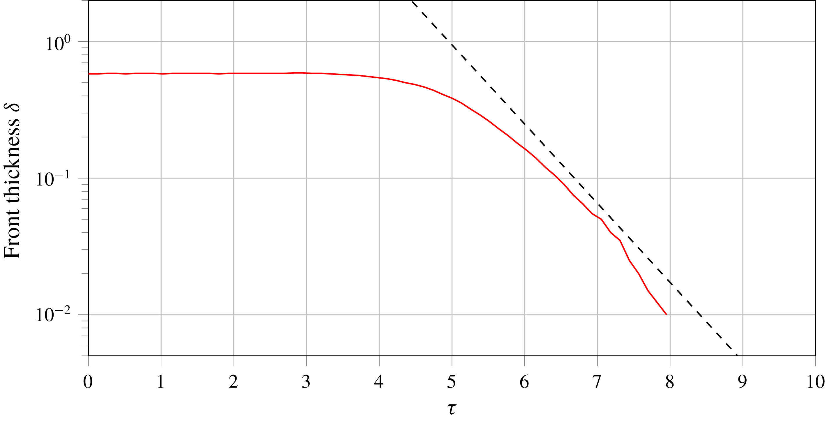
plane acting to sweep the upper part of the tendrils in towards the axis. As a result of this induced motion the front now thins at an exponential rate matching the behaviour predicted by the inviscid model of Davidson et al. (Reference Davidson, Sreenivasan and Aspden2007). Defining the front as the region along the axis where temperature is above
 $0.25~\hat{T}$
we can plot its thickness and confirm that it thins exponentially from
 $\unicode[STIX]{x1D70F}\approx 5.5$
, once roll up into the cap has begun, until
 $\unicode[STIX]{x1D70F}\approx 8$
when the front starts to fade through viscous diffusion. This is shown in figure 10.
Thickness of the temperature front versus time. The dashed line is a line of
 $\unicode[STIX]{x1D6FF}=\text{const.}^{-\unicode[STIX]{x1D70F}}$
for reference.

Another result of our study in support of the model of Davidson et al. (Reference Davidson, Sreenivasan and Aspden2007) is that, after the initial transient and roll up, the velocity of the cap attains an approximately constant value as shown in figure 9. We choose the point (
 $\unicode[STIX]{x1D70F}\approx 7.0$
) at which the cap attains this velocity to mark the end of the transition from buoyant blob to mushroom cap. Although this behaviour was predicted by their model, Davidson et al. (Reference Davidson, Sreenivasan and Aspden2007) noted this as an apparent paradox in their analysis since (2.8) requires impulse to increase linearly in time. For an object of constant volume, this requires the mean velocity to increase linearly in time. They hypothesised that the result might be explained by the generation of
 $\unicode[STIX]{x1D714}_{\unicode[STIX]{x1D703}}$
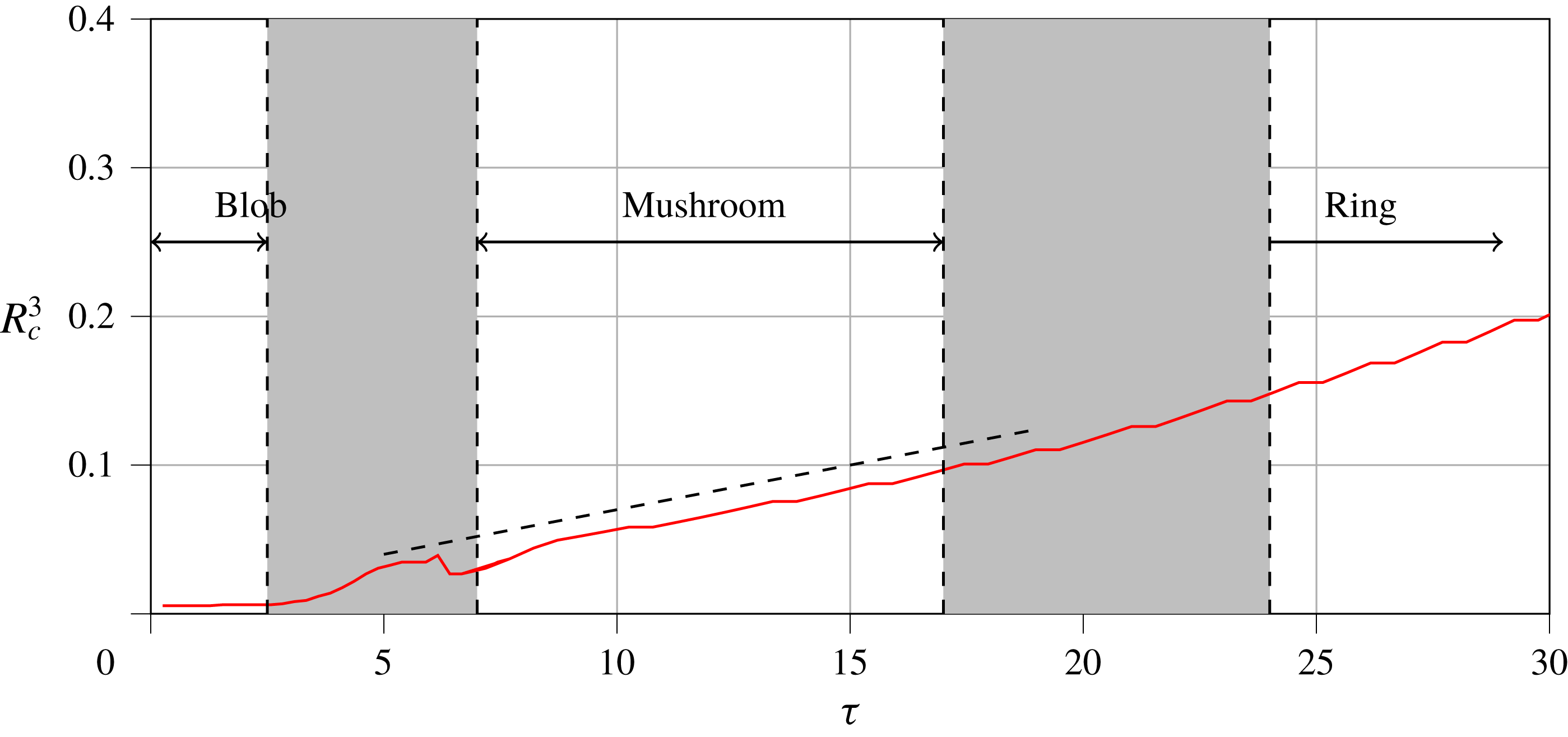
being large lower down in the stem of the mushroom. This is in fact incorrect, as our results show, with a large amount of impulse still being generated in the cap (figure 6). The paradox can instead be explained by the fact that the thermal cap expands radially. Relating linear impulse to momentum in the form
 $\boldsymbol{L}=\int \boldsymbol{u}\,\text{d}V$
, a scaling analysis gives
 $L\sim u_{c}R_{c}^{3}$
, where
 $u_{c}$
is a characteristic cap velocity and
 $R_{c}$
is the outer radius of the cap. Since
 $u_{c}$
tends towards a constant value, we would expect
 $R_{c}$
to scale with
 $t^{1/3}$
in order to be consistent with linearly increasing impulse. This is indeed what we observe in figure 11 plotting
 $R_{c}^{3}$
against
 $\unicode[STIX]{x1D70F}$
.
Value of
 $R_{c}^{3}$
versus
 $\unicode[STIX]{x1D70F}$
for the thermal. The dashed line is a line of
 $R_{c}^{3}\sim \unicode[STIX]{x1D70F}$
for reference.

As the temperature front rapidly thins the source term in (2.12) decreases and so the rate of generation of vorticity also decreases. As a result, the flux
 $\unicode[STIX]{x1D6F7}$
of the cap tends towards a constant value as the front is pulled apart and swept into the lobes. The impulse
 $L$
continues to increase linearly in time, and as such
 $\unicode[STIX]{x1D6FE}$
for the cap decreases at a rate proportional to
 $\unicode[STIX]{x1D70F}^{-1}$
. The wake that is left behind by the cap consists of the trailing tendrils of vorticity bounding a smear of higher temperature fluid. As the mushroom cap moves off ahead of the wake, the height of the wake increases, and so the rate of generation of
 $\unicode[STIX]{x1D6F7}$
in the wake also increases in accordance with (2.12). This is why
 $\unicode[STIX]{x1D6FE}$
for the wake increases over the course of the mushroom stage.
As the mushroom cap progresses it wraps up a significant portion of
 $\unicode[STIX]{x1D714}_{\unicode[STIX]{x1D703}}/r$
from the front and the stem into the lobes that will eventually form the core of the buoyant vortex ring. As a diagnostic we consider the relative strengths of
 $\unicode[STIX]{x1D714}_{\unicode[STIX]{x1D703}}/r$
in the stem and the lobes of the developing ring. The value of
 $\unicode[STIX]{x1D714}_{\unicode[STIX]{x1D703}}/r$
on the axis falls below that at the centre of the forming ring at around
 $\unicode[STIX]{x1D70F}=17$
, marking an end to the mushroom cap and the start of the transition into two separate structures; buoyant vortex ring and wake. We see that the end of this stage is marked by the wake approaching a maximum in
 $\unicode[STIX]{x1D6FE}$
. As the stem becomes thinner, the wake ceases to lengthen along the axis and so the rate of generation of
 $\unicode[STIX]{x1D6F7}$
in the wake remains roughly constant. Since
 $L$
increases at a constant rate
 $\unicode[STIX]{x1D6FE}$
experiences an extremum.
4.4 Stage 3: the buoyant vortex ring
The mushroom cap is subsequently observed to evolve into a buoyant vortex ring that moves off ahead of the trailing wake. We consider initially the motion of this ring after separation using the same methodology as above, before then tying these flow regimes together and examining the separation process.
4.4.1 The mature ring
For a vortex ring containing all of its buoyant material in its core, equation (2.12) tells us that the flux (or circulation) of the ring must remain constant. In addition to this, equation (2.11) tells us that the impulse of the vortex ring must be increasing linearly in time at a rate proportional the thermal energy contained within the core of the ring. Both of these results are in agreement with the analysis of Turner (Reference Turner1957). For a thin-cored vortex ring of mean radius
 $R$
and flux
 $\unicode[STIX]{x1D6F7}$
, the impulse can be approximated (from (2.7) and (2.8)) as
 $L\approx \unicode[STIX]{x03C0}R^{2}\unicode[STIX]{x1D6F7}$
. For this to be consistent with the linearly increasing impulse and constant flux, the ring radius
 $R$
must increase at a rate proportional to
 $t^{1/2}$
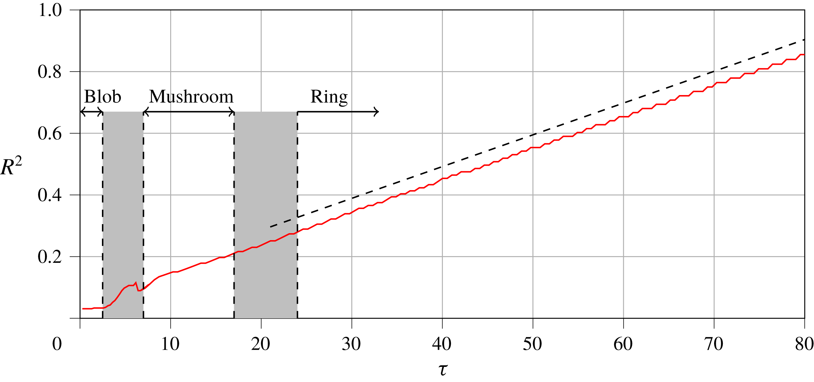
. This is again in agreement with the analysis of Turner (Reference Turner1957) and consistent with the results of our simulations. Figures 6 and 7 show that the flux of the ring remains constant whilst its impulse increases at a constant rate. Plotting
 $R^{2}$
against
 $\unicode[STIX]{x1D70F}$
in figure 12 confirms that the radius of the ring scales as
 $R\sim t^{1/2}$
. As was seen in the cap phase, the seemingly paradoxical result that the ring is decelerating (figure 9) whilst impulse is increasing can be explained by the fact that the radius is increasing, as we now discuss.
Value of
 $R^{2}$
versus
 $\unicode[STIX]{x1D70F}$
for the thermal. The dashed line is a line of
 $R_{c}^{2}\sim \unicode[STIX]{x1D70F}$
for reference.

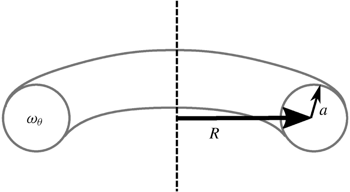
For a vortex ring of the kind sketched in figure 13 with global radius
 $R$
, core radius
 $a$
(
 $a\ll R$
), and a uniform distribution of vorticity
 $\unicode[STIX]{x1D714}_{\unicode[STIX]{x1D703}}$
in the core, the velocity of the ring,
 $V$
, can be calculated (Lamb Reference Lamb1932; Batchelor Reference Batchelor1967; Saffman Reference Saffman1992) as,
 $$\begin{eqnarray}V=\frac{\unicode[STIX]{x1D6F7}}{4\unicode[STIX]{x03C0}R}\left[\ln \left(\frac{8R}{a}\right)-\frac{1}{4}\right].\end{eqnarray}$$
(Of course, during the formation process from a thermal the developing vortex ring is not initially thin cored.) Given the results above, this tells us that buoyant vortex rings must decelerate as they rise, with a rise velocity scaling as
 $t^{-1/2}\ln (t)$
. In addition to this we note the slightly counter-intuitive result (as did Turner Reference Turner1957) that the more buoyant a ring is, the faster it will expand radially and decelerate.
Schematic cross-section of a thin-cored vortex ring.

4.4.2 The separation of the ring from the wake
We now return to consider the separation of the ring from the wake following the end of the mushroom cap phase (around
 $\unicode[STIX]{x1D70F}=17$
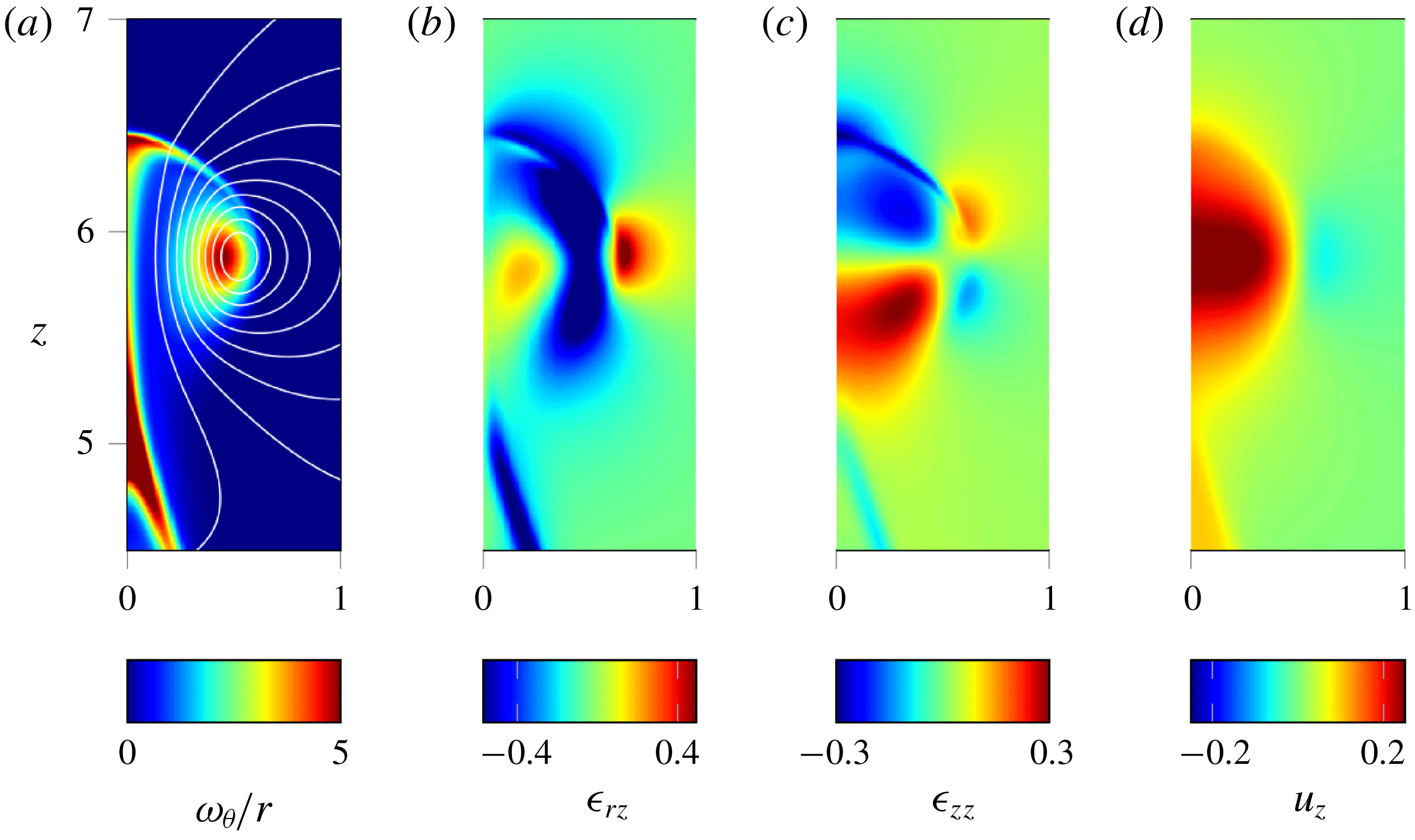
). Let us start by considering more closely the flow between the two separating structures, ring and wake, by looking at the streamlines in figure 14(a). We see that the stem connecting the ring and wake experiences a stretching flow in the axial direction due to the poloidal velocity induced by the ring. Looking at the strain rate plots of figures 14(b) and 14(c) we see that in the stem the dominant strain is
 $\unicode[STIX]{x1D716}_{zz}$
, with positive values from the base of the stem to midway up, consistent with axial stretching. Past the core of the ring the axial strain becomes negative due to the proximity of the cap.
Vorticity, strain-rate components and axial velocity of the thermal at
 $\unicode[STIX]{x1D70F}=19.0$
.

It is important to note here that as the ring and wake separate, the wake rises slower than the ring. This means that the stem connecting the two structures is being stretched from the base of the stem upwards. The vertical velocity (figure 14
d) is largest on the axis at the height of the core of the ring, but small at the base of the stem. So the lower part of the stem is being stretched in the axial direction while squeezed in by the entrained ambient fluid. The effect of this is a rapid reduction in the value of
 $\unicode[STIX]{x1D714}_{\unicode[STIX]{x1D703}}/r$
on the axis of the stem, as we now discuss.
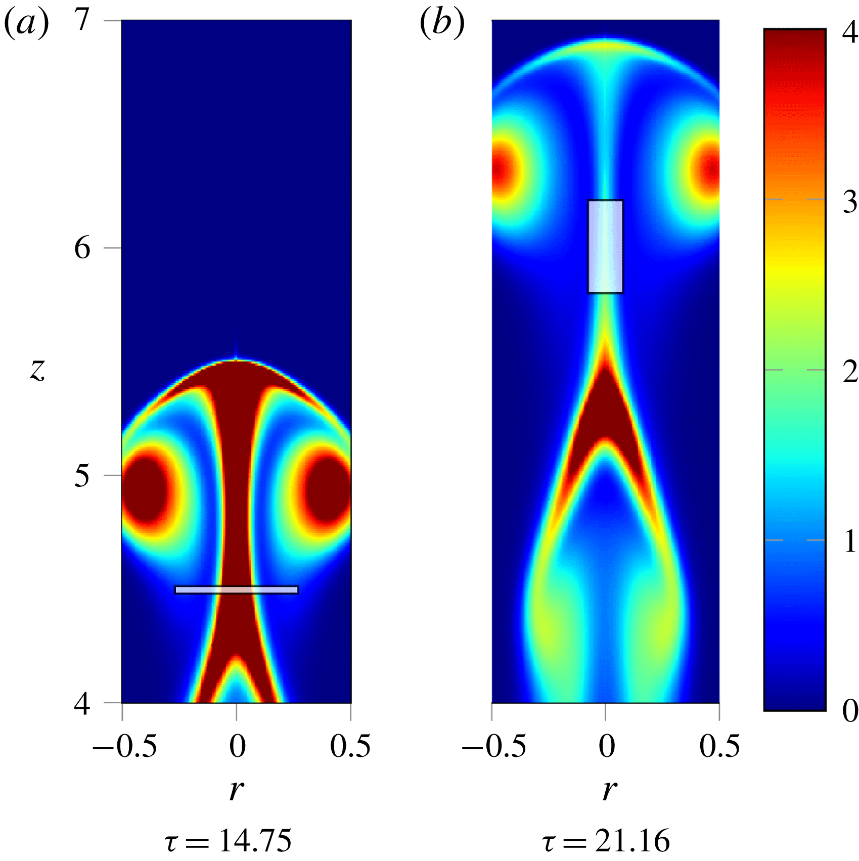
Consider a cylindrical material volume that encloses part of the stem, as shown in figure 15. If we track its progress in the range
 $\unicode[STIX]{x1D70F}=15$
–21, we find that the volume undergoes large axial stretching whilst contracting radially to conserve volume. The start and end points are shown in figure 15. The volume integral of
 $\unicode[STIX]{x1D714}_{\unicode[STIX]{x1D703}}/r$
(
 $\unicode[STIX]{x1D6F7}$
) is plotted in figure 16 and we see that
 $\unicode[STIX]{x1D6F7}$
is approximately conserved, reflecting the relative weakness of the thermal source term in (2.12). Nonetheless, it is clear from our results that the vorticity on the axis of the stem weakens to a point at which the ring can be considered as a separate entity from the wake to which it was once attached. Since the temperature gradients in the stem are small we can approximate (2.3) by
 $$\begin{eqnarray}\frac{\text{D}}{\text{D}t}\left(\frac{\unicode[STIX]{x1D714}_{\unicode[STIX]{x1D703}}}{r}\right)\approx \unicode[STIX]{x1D708}\frac{1}{r^{2}}\unicode[STIX]{x1D6FB}_{\ast }^{2}(r\unicode[STIX]{x1D714}_{\unicode[STIX]{x1D703}}).\end{eqnarray}$$
We now see that as the stem is stretched and thinned by advection, we expect diffusion of
 $\unicode[STIX]{x1D714}_{\unicode[STIX]{x1D703}}/r$
radially outwards. The process of axial stretching therefore helps maintain high gradients in
 $\unicode[STIX]{x1D714}_{\unicode[STIX]{x1D703}}/r$
, enhancing the radial diffusion. Eventually this radial diffusion weakens the centreline value of
 $\unicode[STIX]{x1D714}_{\unicode[STIX]{x1D703}}/r$
sufficiently such that we no longer consider it a connection between ring and wake.
Images of
 $\unicode[STIX]{x1D714}_{\unicode[STIX]{x1D703}}/r$
showing the start and end position of a material volume (white square).

Vorticity flux for a material volume enclosing the stem.

Thus the end of the transition to a buoyant vortex ring occurs when
 $\unicode[STIX]{x1D714}_{\unicode[STIX]{x1D703}}/r$
in the stem connecting the ring to the wake becomes sufficiently weak by diffusion that we can consider them to be two individual structures. Based on this we define the end of the transition period as the time at which
 $\unicode[STIX]{x1D714}_{\unicode[STIX]{x1D703}}/r$
in the stem falls below 20 % of that in the core of the ring. This occurs at
 $\unicode[STIX]{x1D70F}=24$
. By this point the ring has attained a limiting value of
 $\unicode[STIX]{x1D6F7}$
which persists for the remainder of its ascension.
4.5 The wake and multiple vortex rings
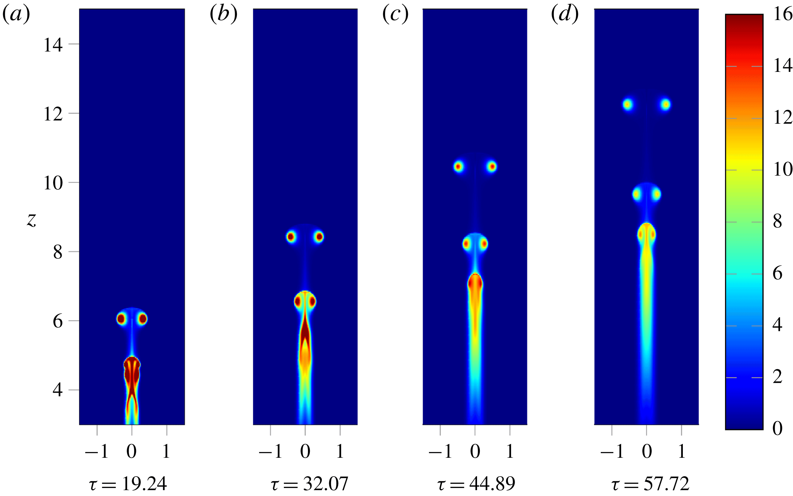
We have discussed the formation of a buoyant vortex ring and its detachment from the wake. Of further interest, however, is the fact that subsequent mushroom caps may form from the thermal wake. These, in turn, may become buoyant rings that detach and follow the first. This behaviour can be seen in both figures 5 and 17. The impulse and flux of the thermal wake is always increasing in time through the same processes as for the initial buoyant blob (2.11) and (2.12). As a result we can have further caps and rings forming that follow the same process of development.
Development of a second vortex ring from the wake left by the separation of the primary vortex ring;
 $\unicode[STIX]{x1D714}_{\unicode[STIX]{x1D703}}/r$
plotted for
 $Re=332$
.

Looking at the wake in figure 4 we see that the radial temperature gradients generate trailing tendrils of vorticity. As these strengthen they become unstable and begin to roll up on themselves, moving in towards the axis. Following these developments further into figure 5 we see the development of the new mushroom cap. The base of the stem that was left by the primary vortex ring is radially stretched to form a new front. The trailing tendrils that wrapped up become the lobes. The cap then proceeds to develop in much the same way as the primary. Looking at
 $\unicode[STIX]{x1D6FE}$
for the wake, we note that the roll up of the tendrils coincides with an increase in
 $\unicode[STIX]{x1D6FE}$
as the vorticity distribution becomes more compact. This reaches a maximum at around
 $\unicode[STIX]{x1D70F}=18$
after which the vorticity distribution expands as it wraps up to form a second mushroom cap.
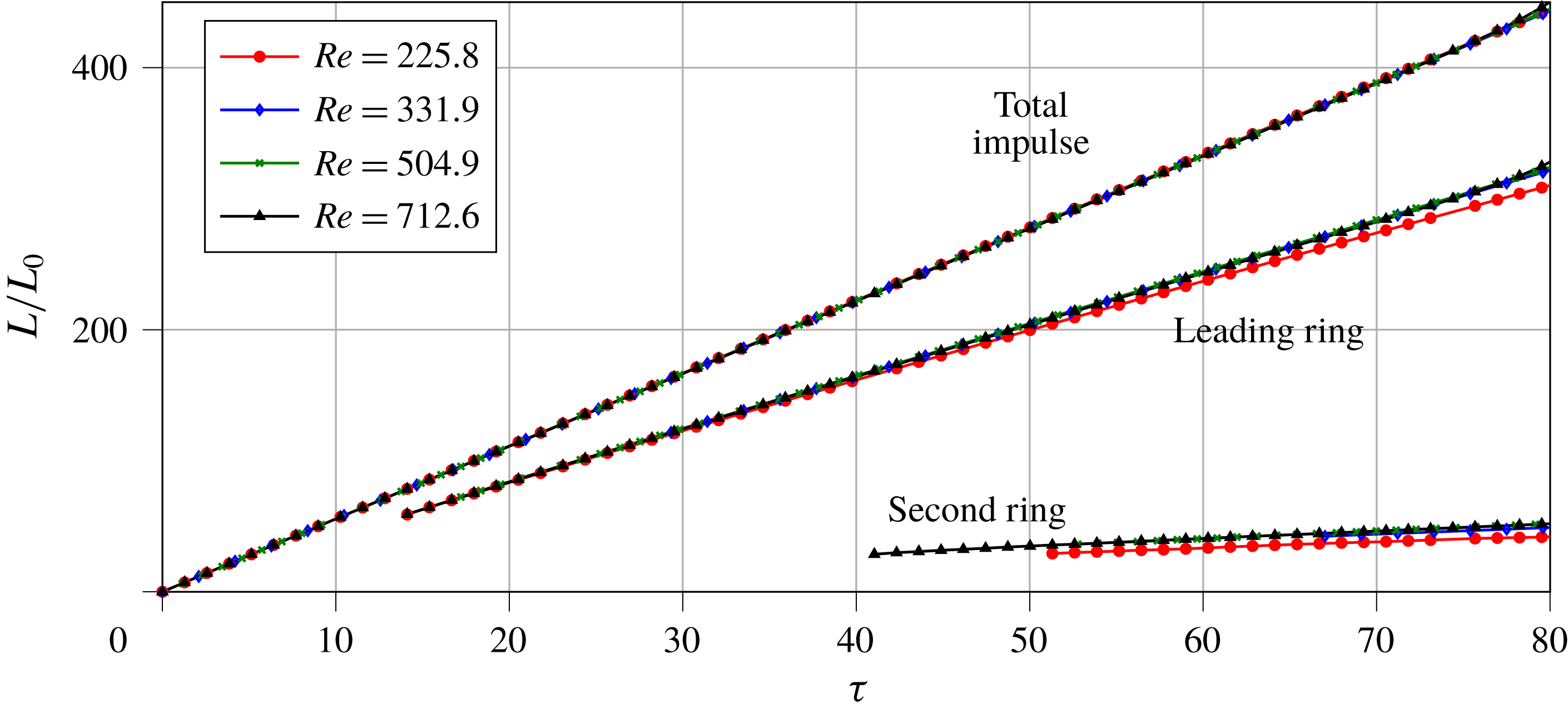
Non-dimensional analysis of impulse for several simulations at
 $Pr=1.0$
and different
 $Re$
.

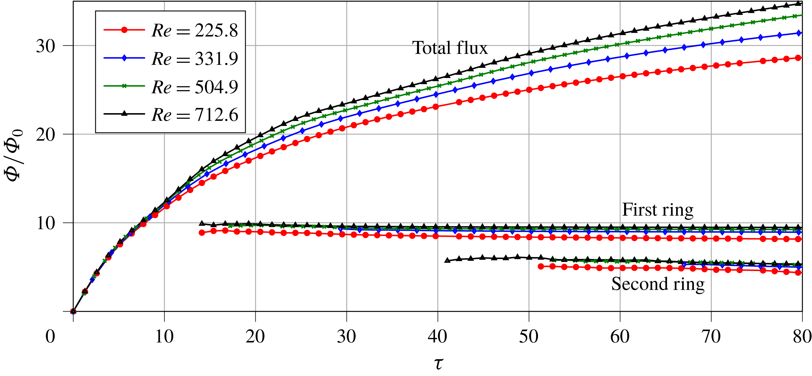
Non-dimensional analysis of flux for several simulations at
 $Pr=1.0$
and different
 $Re$
.

The non-dimensional impulse and flux of the primary and secondary rings are shown in figures 18 and 19 as a function of
 $Re$
. Impulse is significantly reduced in the second ring, whilst the flux is approximately half that of the primary ring. These reductions are, in part, because we are normalising with respect to the initial temperature field, which is not appropriate for the wake. However, it is also clear that the rate of increase of
 $L$
has been reduced in the second ring. To understand this we must consider again (2.11) and (2.12). The rate of generation of impulse scales with the total heat, whilst the rate of flux generation depends upon the heat on the axis. The primary ring wraps up much of the initial heat into its core resulting in it having a much higher rate of impulse generation. An effect of wrapping up into a ring is that hot fluid is removed from the axis, preventing any further increase in the flux of the ring. In contrast to this the wake, though containing less heat than the first ring, remains stretched out along the axis for a much longer period prior to wrapping up to form the second ring. As a result the flux in the wake continues to increase. By the time it separates, the second ring contains around half the flux of the first. Since impulse is much lower than flux for the second ring compared to the first,
 $\unicode[STIX]{x1D6FE}$
is larger. Following wrap up into a second ring and separation from the wake the value of
 $\unicode[STIX]{x1D6FE}$
decreases monotonically as
 $\unicode[STIX]{x1D70F}^{-1}$
, just like the primary ring. The larger value of
 $\unicode[STIX]{x1D6FE}$
for the second ring demands that it is more radially compact than the first.
For some simulations it was observed that further vortex rings could form from the wake of the second provided it did not experience significant diffusive effects in temperature and vorticity. This behaviour can be seen for
 $Re=332$
and
 $Pr=1.0$
in figure 17. The primary ring has moved off ahead by
 $\unicode[STIX]{x1D70F}=32$
and a second cap has begun to form, connected to the lower wake by a stem of vorticity. By
 $\unicode[STIX]{x1D70F}=44$
we see that the stem has weakened as the second ring moves off ahead. Finally, at
 $\unicode[STIX]{x1D70F}=58$
, we see that the two rings are now clearly separate structures ahead of a wake which is capped by a third developing mushroom cap.
5 The influence of
 $Re$
and
$Pr$


Figure 18 shows the impulse of the entire flow and the first and second rings. It is immediately apparent that there is some independence across Reynolds number in this range with the dimensionless impulse of both the first and second rings being almost the same in all cases. Likewise, figure 19 displays good collapse in the final flux for both rings. The total flux of the domain follows the same qualitative pattern for all
 $Re$
, though we see the curves diverge at later times with more flux generated at higher Reynolds numbers.
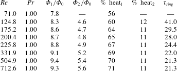
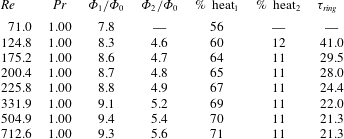
Note that the collapse of impulse requires that each ring contains the same proportion of the initial heat (2.11). This is confirmed by calculating the thermal energy contained in the vortex rings. Table 2 lists the ring properties at
 $\unicode[STIX]{x1D70F}=80$
when the first two vortex rings are separate from the wake. It also contains the parameter
 $\unicode[STIX]{x1D70F}_{ring}$
describing the end of the transition to ring as defined by the criterion outlined above. The value % heat gives the percentage of the initial heat contained within a ring. We see that for a Reynolds number of 332 and above that the first ring consistently contains approximately 70 % of the initial heat, with 11 % in the second ring. The
 $Re=226$
case is slightly lower (67 % and 11 %) but still collapses relatively well with the higher Reynolds number results. This behaviour is not maintained at lower
 $Re$
however. For
 $Re=71$
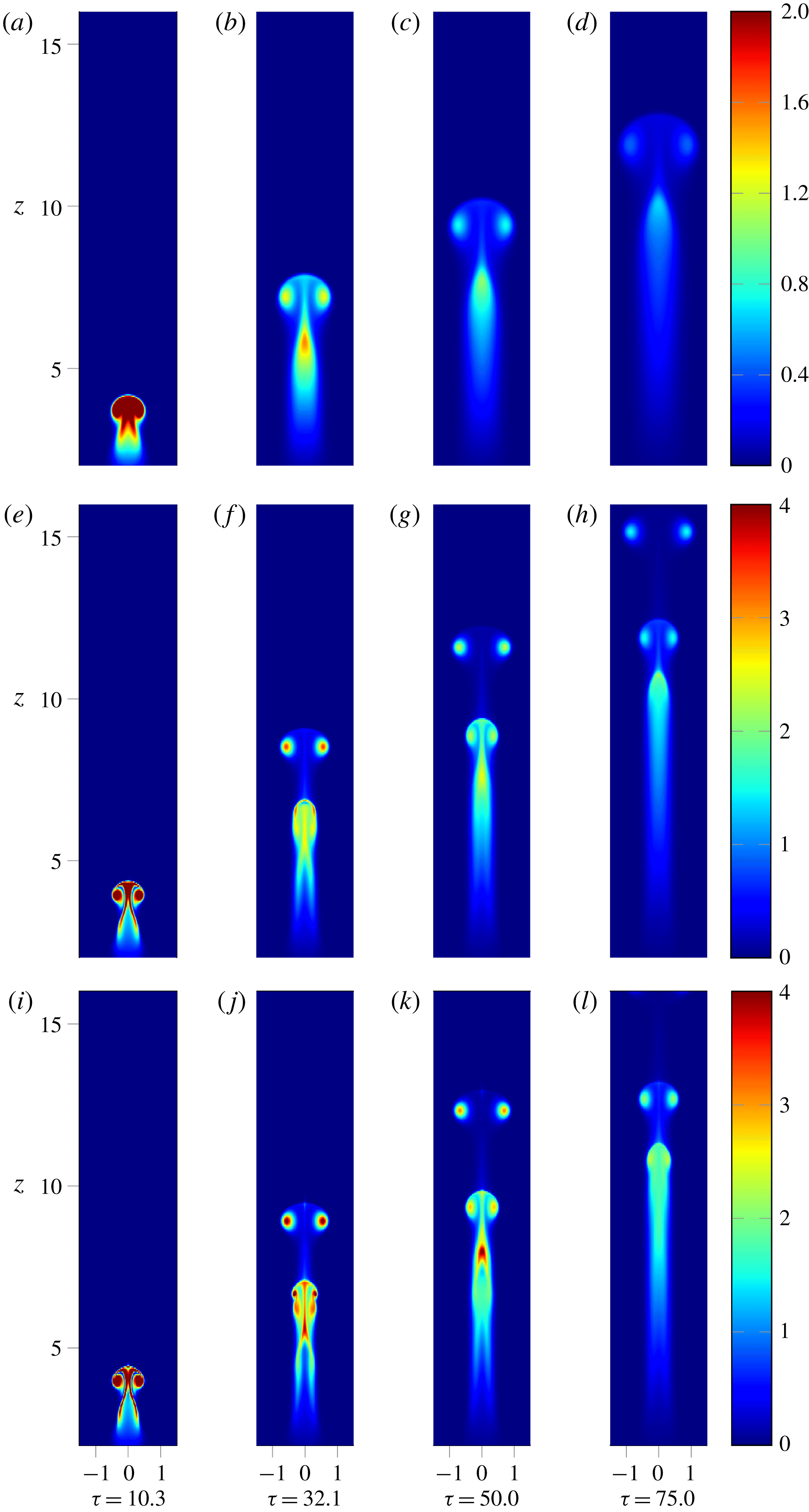
we find that the first ring contains a lower proportion of the total heat and that a second ring does not form at all from the wake as seen in figure 20. This observation would suggest that there is a critical point below which a second vortex ring will not be produced.
Development of
 $\unicode[STIX]{x1D714}_{\unicode[STIX]{x1D703}}/r$
a thermal for
 $Re=71$
(a–d),
 $Re=226$
(e–h) and
 $Re=332$
(i–l). In all cases
 $Pr=1$
. Note different scale for
 $Re=71$
.

Key properties for varying
 $Re$
at
 $\unicode[STIX]{x1D70F}=80$
.
The independence from
 $Re$
at early times can be explained by noting that the characteristic time scale
 $t_{0}$
has no dependence on viscosity. Indeed, following initialisation as a patch of heat in quiescent fluid, the main balance in (2.1) occurs between
 $\unicode[STIX]{x2202}\boldsymbol{u}/\unicode[STIX]{x2202}t$
and
 $-\boldsymbol{g}\unicode[STIX]{x1D6FD}T$
giving the initial acceleration. As the blob begins to lift and roll up into the mushroom cap, the balance transitions to be between
 $\boldsymbol{u}\boldsymbol{\cdot }\unicode[STIX]{x1D735}\boldsymbol{u}$
and
 $-\boldsymbol{g}\unicode[STIX]{x1D6FD}T$
giving a constant cap velocity as discussed. These processes occur between
 $\unicode[STIX]{x1D70F}=0$
–15, i.e. of the order of
 $t_{0}$
. Consider a time scale based on
 $\unicode[STIX]{x1D708}$
as
 $t_{\unicode[STIX]{x1D708}}=l^{2}/\unicode[STIX]{x1D708}$
, which is the relevant time scale for viscous effects to act given smooth initial conditions of length scale
 $l$
. The ratio of this to our characteristic time scale based on buoyancy gives
 $t_{\unicode[STIX]{x1D708}}/t_{0}=Re$
. Based on this we can surmise that, for sufficiently high Reynolds number, viscous effects must only come into play at time scales somewhat longer than it takes for the thermal to wrap up into the mushroom cap. Since this process involves the formation of the core of the vortex ring, the ring is not significantly influenced by viscosity with its properties largely independent of
 $Re$
. These properties are then retained at longer time scales as the ring ascends.
This is not to say that there is no effect however. It is clear from figure 19 that the total flux begins to diverge from around
 $\unicode[STIX]{x1D70F}=15$
. Since the primary ring displays a good collapse in
 $\unicode[STIX]{x1D6F7}/\unicode[STIX]{x1D6F7}_{0}$
the source of this discrepancy must lie in the wake. Furthermore we know that, once formed, the ring cannot contribute to the generation of
 $\unicode[STIX]{x1D6F7}$
since all the heat is contained in the core (2.12). It can be seen from figure 20 that as Reynolds number decreases,
 $\unicode[STIX]{x1D714}_{\unicode[STIX]{x1D703}}/r$
in the wake becomes weaker and more diffuse. To understand why this is we must consider (2.3) and (2.12), and also note that these results are all for a Prandtl number of 1. Therefore as Reynolds number falls, so does the Péclet number, and so the effects of thermal diffusivity increase. Since the initial condition is quiescent fluid, we can disregard the effects of viscosity at early times when there is little motion. The same cannot be said for thermal diffusion however. Immediately following initialisation thermal diffusion will act to spread out the heat, reducing the radial temperature gradients that generate vorticity (2.3). For low Reynolds number (
 $Re=71$
) this has an impact early on, with significantly lower
 $\unicode[STIX]{x1D714}_{\unicode[STIX]{x1D703}}/r$
across the entire thermal. The ring also contains a noticeably lower proportion of the initial heat. We noted above that, once formed, the ring maintains its flux so the main effects of thermal diffusion at later times must occur in the wake. When thermal diffusion is larger, the warm wake will expand and temperature gradients reduce. As a result, the generation of
 $\unicode[STIX]{x1D714}_{\unicode[STIX]{x1D703}}/r$
is reduced. This leads to the diverging lines of
 $\unicode[STIX]{x1D6F7}/\unicode[STIX]{x1D6F7}_{0}$
in figure 19 and weaker
 $\unicode[STIX]{x1D714}_{\unicode[STIX]{x1D703}}/r$
in the wake.
In order to isolate the effects of thermal diffusivity we examined the effect of varying Prandtl number between 0.1 and 2.0 for a fixed Reynolds number of 225.8. This introduces a second diffusive time scale based upon the thermal diffusivity,
 $t_{\unicode[STIX]{x1D6FC}}$
, defined in a similar way to
 $t_{\unicode[STIX]{x1D708}}$
. For
 $Pr=1.0$
,
 $t_{\unicode[STIX]{x1D6FC}}=t_{\unicode[STIX]{x1D708}}$
, so when the viscous time scale is long in comparison to the formation time, so is
 $t_{\unicode[STIX]{x1D6FC}}$
. Therefore we deduce that for
 $Pr>1$
there should be no significant difference in the results. However, for Prandtl numbers below 1,
 $t_{\unicode[STIX]{x1D6FC}}$
may become comparable to the formation time even when
 $t_{\unicode[STIX]{x1D708}}$
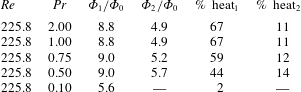
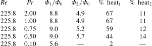
remains large. In these cases we find that diffusive effects interrupt the formation process by smearing out heat as discussed above. Table 3 lists the key values for a range of Prandtl numbers at a fixed
 $\unicode[STIX]{x1D70F}$
. As expected, for
 $Pr>1$
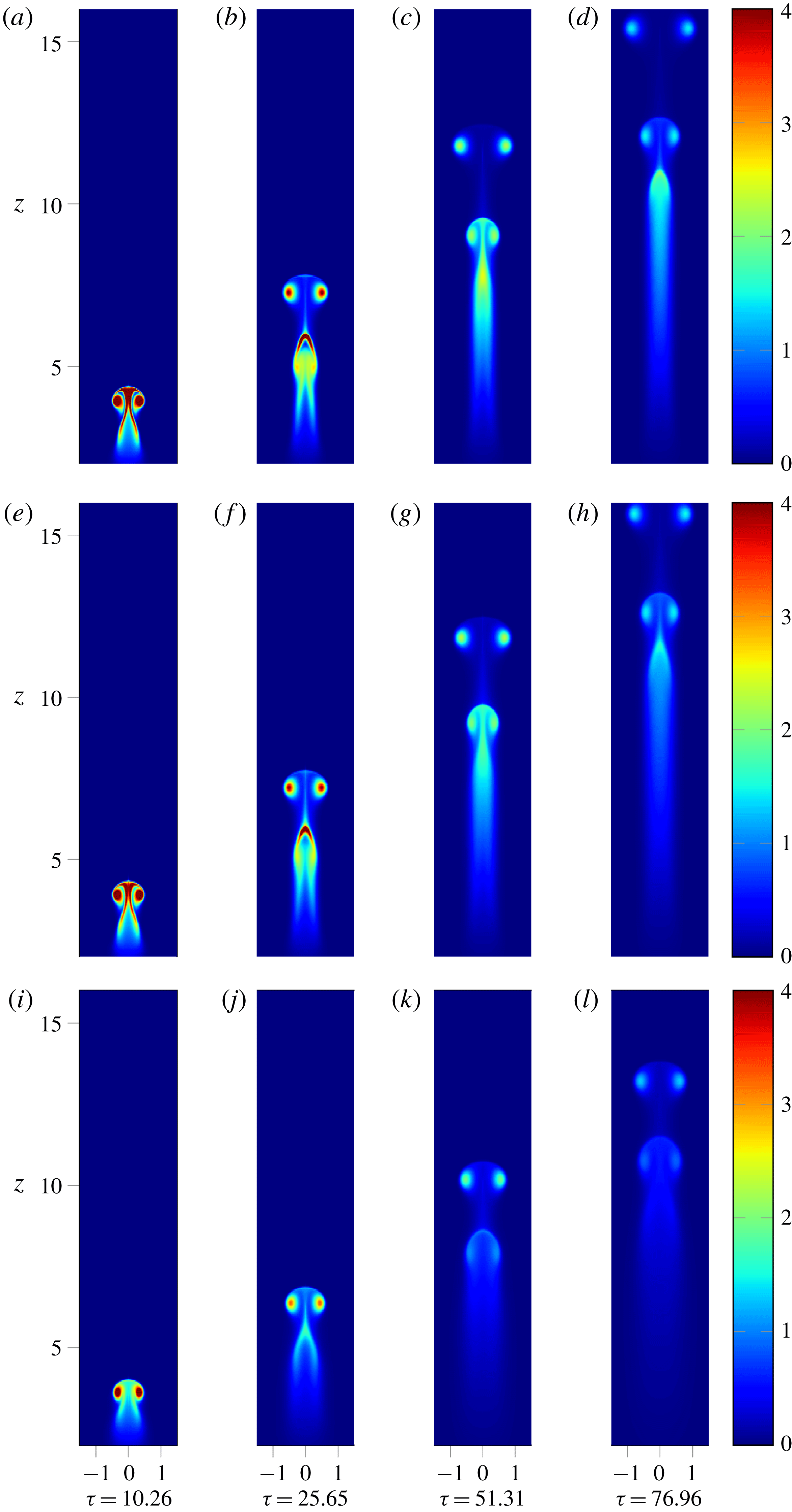
the properties of the first and second ring are identical, with formation occurring before diffusive effects have time to act. For lower Prandtl numbers the first vortex ring contains less of the initial heat and both the rings and wake are weaker in
 $\unicode[STIX]{x1D714}_{\unicode[STIX]{x1D703}}/r$
. This is illustrated in figure 21. For the case
 $Pr=0.1$
it becomes particularly apparent how diffusion destroys the sharp radial gradients in temperature that lead to the generation of vorticity tendrils and secondary rings. The proportion of heat contained in the second ring actually increases as
 $Pr$
falls, though this likely results from the fact that the wake is left with increased heat. For
 $Pr=0.1$
although a second cap is developing at our chosen value of
 $\unicode[STIX]{x1D70F}$
it has not progressed enough for its values to be well defined.
Development of
 $\unicode[STIX]{x1D714}_{\unicode[STIX]{x1D703}}/r$
a thermal
 $Re=225$
for
 $Pr=1.0$
(a–d),
 $Pr=0.5$
(e–h) and
 $Pr=0.1$
(i–l).

Key properties for varying
 $Pr$
at
 $\unicode[STIX]{x1D70F}=80$
.
Since viscous effects have little impact at the early stages of the development process we see that, provided the effects of heat transfer are also negligible, the end of the blob phase (constant acceleration), start of the cap phase (constant velocity,
 $R^{3}\sim t$
) and end of the cap phase (stem weaker than lobes) all develop according to a universal time scale. There is some discrepancy at the end of the transition to the ring however which is recorded in table 2 as
 $\unicode[STIX]{x1D70F}_{ring}$
. We find that as
 $Re$
falls, the time for
 $\unicode[STIX]{x1D714}_{\unicode[STIX]{x1D703}}/r$
in the stem to fall below 20 % of that in the core increases. Saffman (Reference Saffman1970) examined the effect of viscosity on thin-cored vortex rings. He showed that diffusion of vorticity will cause the core radius
 $a$
to increase at rate
 $\left(4\unicode[STIX]{x1D708}t\right)^{1/2}$
. This is accompanied by a decrease in peak vorticity. The rise velocity of (4.1) becomes
 $$\begin{eqnarray}V_{visc.}=\frac{\unicode[STIX]{x1D6F7}}{4\unicode[STIX]{x03C0}R}\left[\ln \left(\frac{8R}{\sqrt{4\unicode[STIX]{x1D708}t}}\right)-0.558\right],\end{eqnarray}$$
indicating that the more viscous a fluid, the slower a vortex ring (of a given buoyancy) will ascend. As a result rings of a lower Reynolds number will rise more slowly, and thus the stem connecting the ring to the wake will be stretched more slowly. Since the stretching process encourages the diffusion of
 $\unicode[STIX]{x1D714}_{\unicode[STIX]{x1D703}}/r$
away from the axis we might expect that faster rising rings separate more quickly.
6 Conclusions
We have characterised the behaviour of the flow resulting from a buoyant perturbation in an otherwise quiescent fluid. To do this we broke the flow down into three key stages; the buoyant blob, the mushroom cap and the buoyant vortex ring. We also looked at the evolution of the wake left behind by the ring. Though these phenomena have previously been discussed individually, we believe that this is the first time the development from buoyant blob to mushroom cap and on into a buoyant vortex ring has been treated as a continuous process.
The equations we have used can link the results of Shlein for buoyant blobs to those of Turner for buoyant vortex rings. By examining the evolution of the impulse, flux and
 $\unicode[STIX]{x1D6FE}$
, we identified key points in the development of the thermal such as the roll up of the cap and separation of the ring from the wake. We have taken a closer look at the mushroom cap stage, examining and explaining the scaling of cap radius with time (
 $R^{3}\sim t$
), and providing validation for the model presented by Davidson et al. (Reference Davidson, Sreenivasan and Aspden2007). We have also shown that this approach gives equivalent results for buoyant vortex rings when compared to the analysis performed by Turner (Reference Turner1957). We find that radial expansion of the slowing ring (
 $R^{2}\sim t$
) is required for compatibility with linearly increasing impulse. As a result of this new approach we have also been able to shed light on a number of unsolved problems from previous works. We show that the constant acceleration of the buoyant blob observed by Shlien (Reference Shlien1976) can be explained by considering the dynamic balance at early times. We also resolved the apparent paradox raised by Davidson et al. (Reference Davidson, Sreenivasan and Aspden2007) by noting that the radial expansion that occurs during the mushroom cap phase allows the impulse to continue increasing whilst the cap tends towards a constant velocity.
Exploring the effect of Reynolds and Prandtl number, we have shown that the early stages of development are key in determining the final properties of the buoyant vortex ring. We found that there is an independence in properties across a range of Reynolds numbers due to cap formation occurring on a time scale where viscosity has no significant effect. The independence of impulse arises from the fact that, when forming, the ring always wraps up the same proportion of the initial heat into its core. In contrast we find that the effects of thermal diffusion can have a significant effect on the early stages of development when there is little motion. Thermal diffusion acts to smooth out the temperature field, inhibiting the generation of vorticity.
Finally, by considering the behaviour of the wake left behind by the ring, we show that the formation of secondary vortex rings is entirely to be expected. Buoyant fluid left behind by the first ring can undergo a similar process, forming a cap and eventually a secondary buoyant vortex ring that separates to follow the first. Again, the effects of thermal diffusion can become noticeable in the wake where the smoothing of temperature gradients interferes with vorticity generation and inhibits the production of successive rings.
Acknowledgements
J. A. would like to thank EPSRC for funding this work through a CUED departmental award (reference no. 1608617). The authors would also like to thank J. Perry for assistance in implementing some aspects of the numerics, and G. R. Hunt for several helpful comments.
Appendix A. Scaling analysis at early times
Given that
 $\boldsymbol{u}$
is small for small
 $t$
we can approximate (2.1) as,
 $$\begin{eqnarray}\frac{\unicode[STIX]{x2202}\boldsymbol{u}}{\unicode[STIX]{x2202}t}\sim \boldsymbol{g}\unicode[STIX]{x1D6FD}T\;\Longrightarrow \;\boldsymbol{u}\sim \boldsymbol{g}\unicode[STIX]{x1D6FD}Tt.\end{eqnarray}$$
Based on this we can quantify the relative sizes of the advective terms in both (2.1) and (2.2) as,
 $$\begin{eqnarray}\displaystyle \frac{\displaystyle \frac{\unicode[STIX]{x2202}\boldsymbol{u}}{\unicode[STIX]{x2202}t}}{\boldsymbol{u}\boldsymbol{\cdot }\unicode[STIX]{x1D735}\boldsymbol{u}}\sim \frac{\displaystyle \frac{\unicode[STIX]{x2202}T}{\unicode[STIX]{x2202}t}}{\boldsymbol{u}\boldsymbol{\cdot }\unicode[STIX]{x1D735}T} & {\sim} & \displaystyle \frac{l}{ut}\nonumber\\ \displaystyle & {\sim} & \displaystyle \frac{l}{t(g\unicode[STIX]{x1D6FD}Tt)}\nonumber\\ \displaystyle & {\sim} & \displaystyle \frac{l^{2}}{U^{2}t^{2}}.\end{eqnarray}$$
Hence we can define a time scale over which we may regard the advective terms to be small as follows:
 $$\begin{eqnarray}\displaystyle \left.\begin{array}{@{}c@{}}\displaystyle \frac{\unicode[STIX]{x2202}\boldsymbol{u}}{\unicode[STIX]{x2202}t}\gg \boldsymbol{u}\boldsymbol{\cdot }\unicode[STIX]{x1D735}\boldsymbol{u}\\ \displaystyle \frac{\unicode[STIX]{x2202}T}{\unicode[STIX]{x2202}t}\gg \boldsymbol{u}\boldsymbol{\cdot }\unicode[STIX]{x1D735}T\end{array}\right\}\quad \text{for}~t\ll \frac{l}{U}. & & \displaystyle\end{eqnarray}$$
Now we turn our attention to the thermal diffusion. Based on the above analysis we can approximate (2.2) for small
 $t$
as,
 $$\begin{eqnarray}\frac{\unicode[STIX]{x2202}T}{\unicode[STIX]{x2202}t}\sim \unicode[STIX]{x1D6FC}\unicode[STIX]{x1D6FB}^{2}T\sim \unicode[STIX]{x1D6FC}\frac{T}{l^{2}}.\end{eqnarray}$$
A scaling analysis then gives
 $$\begin{eqnarray}\frac{\unicode[STIX]{x0394}T}{\hat{T}}\sim \frac{\displaystyle \frac{\unicode[STIX]{x2202}T}{\unicode[STIX]{x2202}t}t}{\hat{T}}\sim \frac{\displaystyle \unicode[STIX]{x1D6FC}\frac{\hat{T}}{l^{2}}t}{\hat{T}}\sim \frac{\unicode[STIX]{x1D6FC}t}{l^{2}}\sim \left(\frac{l_{\unicode[STIX]{x1D6FC}}}{l}\right)^{2},\end{eqnarray}$$
where
 $\unicode[STIX]{x0394}T$
is a typical change in temperature and
 $l_{\unicode[STIX]{x1D6FC}}$
is the diffusion length. In order to regard thermal diffusion as negligible (
 $\unicode[STIX]{x0394}T/\hat{T}\ll 1$
) we therefore require,
 $$\begin{eqnarray}\frac{\unicode[STIX]{x1D6FC}(l/U)}{l^{2}}\ll 1,\end{eqnarray}$$
or alternatively
 $$\begin{eqnarray}Pe=\frac{Ul}{\unicode[STIX]{x1D6FC}}\gg 1,\end{eqnarray}$$
where
 $Pe$
is the Péclet number.