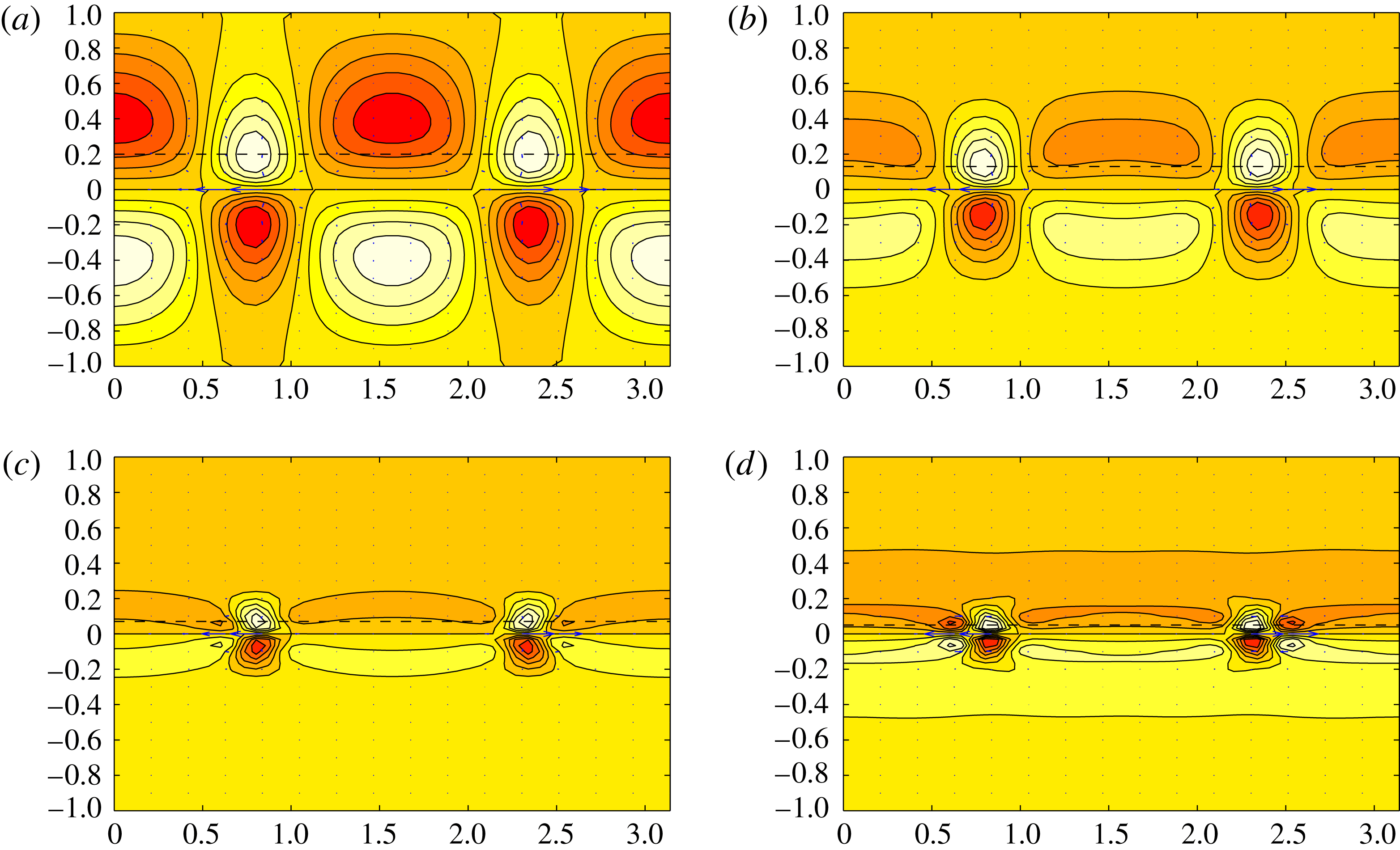
1 Introduction
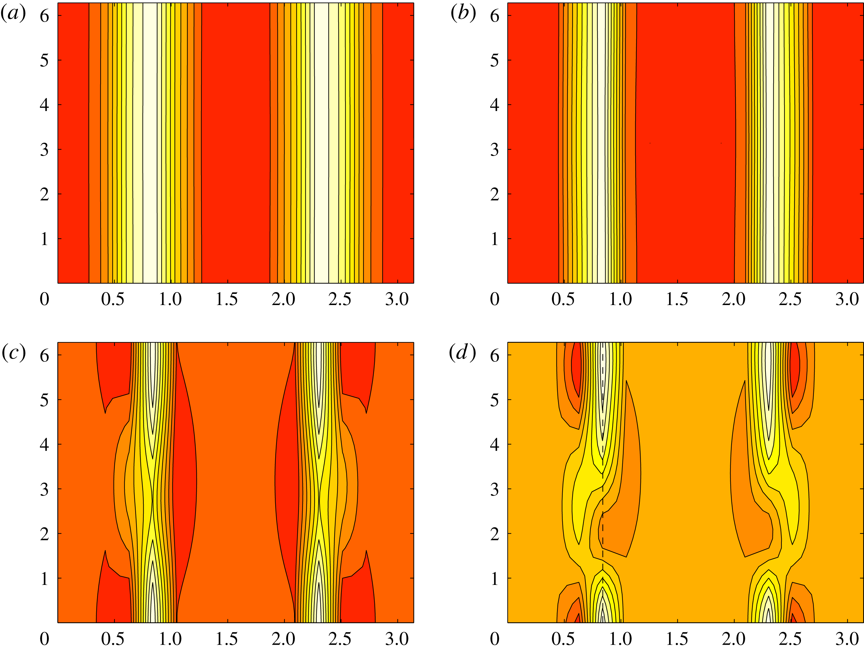
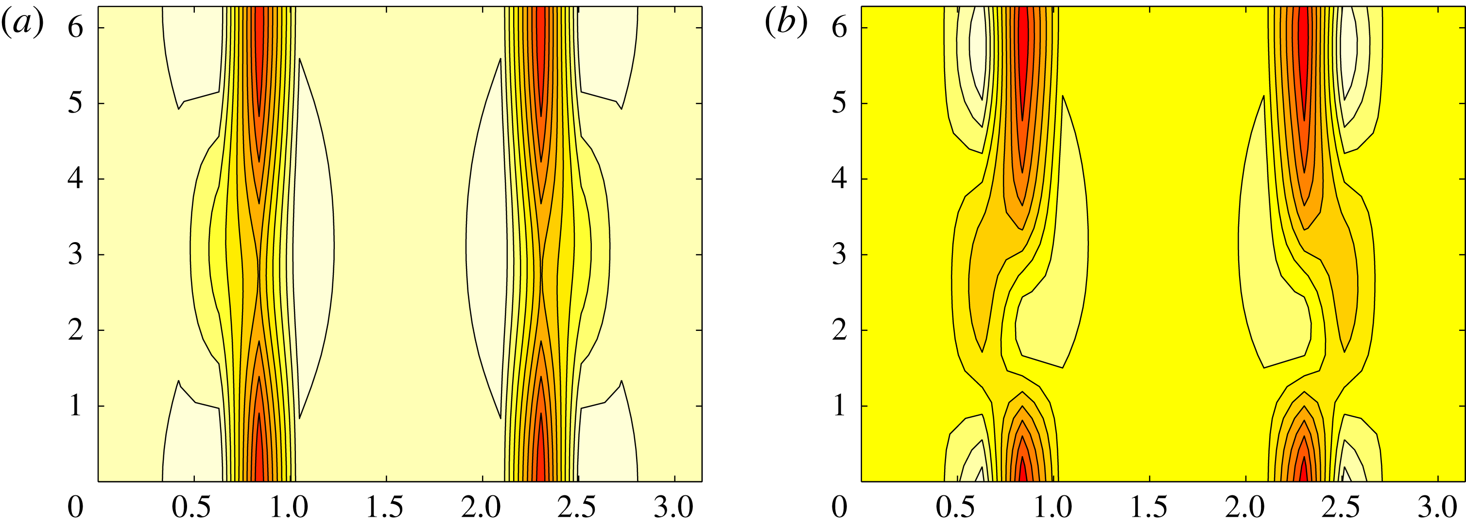
Our understanding of transition to turbulence in linearly stable shear flows such as plane Couette flow (PCF) and pipe flow has experienced a considerable step forward over the last 25 years based upon the realisation that such flows have many alternative unstable solutions such as equilibria, travelling waves and periodic states (Nagata Reference Nagata1990; Waleffe Reference Waleffe1998; Faisst & Eckhardt Reference Faisst and Eckhardt2003; Wedin & Kerswell Reference Wedin and Kerswell2004). These states, which start to populate phase space at some critical Reynolds number and quickly proliferate as the Reynolds number increases, eventually produce a sufficiently tangled structure of stable and unstable manifolds in phase space to act as a scaffold for the observed complex dynamics (Kerswell Reference Kerswell2005; Eckhardt et al. Reference Eckhardt, Schneider, Hof and Westerweel2007; Gibson & Cvitanović Reference Gibson and Cvitanović2010; Kawahara, Uhlmann & van Veen Reference Kawahara, Uhlmann and van Veen2012). These states (variously referred to as simple invariant solutions or exact coherent structures (ECS)) can either be embedded in the laminar–turbulent boundary (Wang et al. Reference Wang, Gibson and Waleffe2007; Duguet, Willis & Kerswell Reference Duguet, Willis and Kerswell2008) or sit in the basin of attraction of the turbulent state with some buried in the turbulent attractor itself (Kerswell & Tutty Reference Kerswell and Tutty2007; Gibson, Halcrow & Cvitanović Reference Gibson, Halcrow and Cvitanović2008). As a consequence, properties of the ECS have something to say about how transition is triggered (Viswanath & Cvitanović Reference Viswanath and Cvitanović2009; Duguet, Brandt & Larsson Reference Duguet, Brandt and Larsson2010; Pringle et al. Reference Pringle, Willis and Kerswell2012), the subsequent transitional process (Itano & Toh Reference Itano and Toh2001; Skufca, Yorke & Eckhardt Reference Skufca, Yorke and Eckhardt2006; Schneider, Eckhardt & Yorke Reference Schneider, Eckhardt and Yorke2007; Mellibovsky et al. Reference Mellibovsky, Meseguer, Schneider and Eckhardt2009) and features of the turbulent state itself (e.g. Kawahara & Kida Reference Kawahara and Kida2001, Hof et al. Reference Hof, van Doorne, Westerweel, Nieuwstadt, Faisst, Eckhardt, Wedin, Kerswell and Waleffe2004, Viswanath Reference Viswanath2007, Gibson et al. Reference Gibson, Halcrow and Cvitanović2008, Chandler & Kerswell Reference Chandler and Kerswell2013, Willis, Cvitanovic & Avila Reference Willis, Cvitanovic and Avila2013, Lucas & Kerswell Reference Lucas and Kerswell2015).
The motivation for this study is to extend these investigations to stably stratified shear flow, which is the generic situation in environmental and geophysical flows (e.g. oceanic flows are almost always stably stratified – Thorpe Reference Thorpe2007). While there has been previous work on unstably stratified shear flow – Rayleigh–Bénard convection with imposed shear (Clever, Busse and Kelly Reference Clever, Busse and Kelly1977; Clever & Busse Reference Clever and Busse1992), internally heated shear flow (Generalis & Nagata Reference Generalis and Nagata2003) and natural convection with imposed shear (Hall Reference Hall2012) – the only work in computing ECS for stable stratification is that of Clever & Busse (Reference Clever and Busse1992, Reference Clever, Busse, Egbers and Pfister2000), who established that Nagata’s (Reference Nagata1990) now famous first solution in PCF could be continued back to Rayleigh–Bénard convection with shear. This lack of attention might well be because stable stratification is perceived as a universally stabilising influence, although this is now appreciated as an oversimplification (Howard & Maslowe Reference Howard and Maslowe1973; Huppert 1973; Davey & Reid Reference Davey and Reid1977), or because introducing stratification increases the dimension of parameter space from a very manageable 1 (
 $Re$
, the Reynolds number) to a more daunting 3 (
 $Re$
,
 $Ri_{b}$
and
 $Pr$
, where the bulk Richardson and Prandtl numbers are defined below).
Mathematically, rather than being a complication, stratification actually presents an opportunity to embed the now well-studied problem of PCF into a larger framework which can smoothly connect to the even more well-studied problem of Rayleigh–Bénard convection. Physically, another interesting aspect of adding further parameters to the problem is the increased dimension of any laminar boundary in parameter space. Ignoring the Prandtl number (set to unity throughout this study) still leaves two parameters and then a one-dimensional laminar–turbulent boundary, as opposed to the zero-dimensional situation in unstratified PCF (e.g. see figure 1 of Deusebio, Caulfield & Taylor Reference Deusebio, Caulfield and Taylor2015). Understanding exactly how this boundary behaves for large
 $Re$
is an important open problem in stratified turbulence which has obvious implications for parametrising turbulence in ocean, atmosphere and climate models. In particular, if
 $Ri_{b}^{c}(Re)$
defines the laminar–turbulent boundary, does
 $Ri_{b}^{c}$
tend to zero or not as
 $Re\rightarrow \infty$
? Having an asymptotic regime where the flow is always transitional opens up interesting new opportunities to probe the complex dynamics involved. An obvious place to start addressing this question is to understand where in parameter space ECS exist, since they are currently viewed as necessary precursors for turbulent dynamics. This is the focus of the current study.
The plan of the paper is as follows. Section 2 formulates the problem of stratified plane Couette flow and discusses the numerical methods to be used. In § 3.1, an initial investigation is described which identifies where the laminar–turbulent boundary is in the
 $Re{-}Ri_{b}$
plane for two typical (small box) geometries. Section 3.2 then describes the results of edge tracking in a variety of geometries aimed at uncovering new ECS. Two already known, albeit now stratified, ECS are repeatedly found – EQ7 and EQ7-1 in the nomenclature of Gibson & Brand (Reference Gibson and Brand2014). In § 3.3 these are continued around in
 $Re{-}Ri_{b}$
parameter space, including into negative
 $Ri_{b}$
(unstable stratification), along with Nagata’s (Reference Nagata1990) first solution in PCF. In § 3.4 the behaviour of EQ7 (which is most robust with respect to stable stratification) is examined at large
 $Re$
. A stratified version of the vortex wave interaction asymptotics of Hall & Sherwin (Reference Hall and Sherwin2010) is then discussed for very weak stratification. As the stratification is increased, a second regime is suggested by the numerical solutions which show EQ7 spanwise localisation and amounts to a stratified version of the boundary region equations of Deguchi, Hall & Walton (Reference Deguchi, Hall and Walton2013). A third, ultimate regime is also discussed in which the ECS are fully localised. Section 4 provides a final discussion of the results and future directions for further research.
2 Formulation
2.1 Stratified plane Couette flow
We consider the usual plane Couette flow set-up of two (horizontal) parallel plates separated by a distance
 $2h$
, with the top plate moving at
 $U\hat{\boldsymbol{x}}$
and the bottom plate moving at
 $-U\hat{\boldsymbol{x}}$
. Dirichlet boundary conditions are imposed on the density field (Armenio & Sarkar Reference Armenio and Sarkar2002; Garcia-Villalba & del Alamo Reference Garcia-Villalba and del Alamo2011): the fluid density is
 $\unicode[STIX]{x1D70C}_{0}-\unicode[STIX]{x1D6E5}_{\unicode[STIX]{x1D70C}}$
at the top plate and
 $\unicode[STIX]{x1D70C}_{0}+\unicode[STIX]{x1D6E5}_{\unicode[STIX]{x1D70C}}$
at the bottom plate (gravity
 $g$
is normal to the plates and directed downwards from the top plate to the bottom plate). Using the Boussinesq approximation (
 $\unicode[STIX]{x1D6E5}_{\unicode[STIX]{x1D70C}}\ll \unicode[STIX]{x1D70C}_{0}$
), the governing equations can be non-dimensionalised using
 $U$
,
 $h$
and
 $\unicode[STIX]{x1D6E5}_{\unicode[STIX]{x1D70C}}$
to give
 $$\begin{eqnarray}\displaystyle & \displaystyle {\displaystyle \frac{\unicode[STIX]{x2202}\boldsymbol{u}}{\unicode[STIX]{x2202}t}}+\boldsymbol{u}\boldsymbol{\cdot }\unicode[STIX]{x1D735}\boldsymbol{u}=-\unicode[STIX]{x1D735}p-Ri_{b}\;\unicode[STIX]{x1D70C}\;\hat{\boldsymbol{y}}+{\displaystyle \frac{1}{Re}}\unicode[STIX]{x1D6FB}^{2}\boldsymbol{u}, & \displaystyle\end{eqnarray}$$
 $$\begin{eqnarray}\displaystyle & \displaystyle \unicode[STIX]{x1D735}\boldsymbol{\cdot }\boldsymbol{u}=0, & \displaystyle\end{eqnarray}$$
 $$\begin{eqnarray}\displaystyle & \displaystyle {\displaystyle \frac{\unicode[STIX]{x2202}\unicode[STIX]{x1D70C}}{\unicode[STIX]{x2202}t}}+\boldsymbol{u}\boldsymbol{\cdot }\unicode[STIX]{x1D735}\unicode[STIX]{x1D70C}={\displaystyle \frac{1}{Re\;Pr}}\unicode[STIX]{x1D6FB}^{2}\unicode[STIX]{x1D70C}, & \displaystyle\end{eqnarray}$$
where the bulk Richardson number
 $Ri_{b}$
, Reynolds number
 $Re$
and Prandtl number
 $Pr$
(always set to 1 in this study) are respectively defined as:
 $$\begin{eqnarray}Ri_{b}:={\displaystyle \frac{\unicode[STIX]{x1D6E5}_{\unicode[STIX]{x1D70C}}\hspace{2.22198pt}g\,h}{\unicode[STIX]{x1D70C}_{0}\,U^{2}}},\quad Re:={\displaystyle \frac{U\,h}{\unicode[STIX]{x1D708}}},\quad Pr:={\displaystyle \frac{\unicode[STIX]{x1D708}}{\unicode[STIX]{x1D705}}}.\end{eqnarray}$$
Here
 $\boldsymbol{u}=(u,v,w)$
is the velocity field,
 $\unicode[STIX]{x1D705}$
is the thermal diffusivity, the total dimensional density is
 $\unicode[STIX]{x1D70C}_{0}+\unicode[STIX]{x1D6E5}_{\unicode[STIX]{x1D70C}}$
,
 $p$
is the pressure and
 $\unicode[STIX]{x1D708}$
is the kinematic viscosity. The boundary conditions are then
 $$\begin{eqnarray}u(x,\pm 1,z,t)=\pm 1\quad \text{and}\quad \unicode[STIX]{x1D70C}(x,\pm 1,z,t)=\mp 1,\end{eqnarray}$$
which admit the steady one-dimensional solution
 $$\begin{eqnarray}\boldsymbol{u}=y\,\hat{\boldsymbol{x}}\quad \text{and}\quad \unicode[STIX]{x1D70C}=-y.\end{eqnarray}$$
The (possibly large) disturbance fields away from this basic state,
 $$\begin{eqnarray}\hat{\boldsymbol{u}}(x,y,z,t)=\boldsymbol{u}-y\,\hat{\boldsymbol{x}},\quad \hat{\unicode[STIX]{x1D70C}}(x,y,z,t)=\unicode[STIX]{x1D70C}+y,\end{eqnarray}$$
conveniently satisfy homogeneous boundary conditions at
 $y=\pm 1$
. Periodic boundary conditions are used in both the streamwise (
 $x$
) and spanwise (
 $z$
) directions over wavelengths
 $L_{x}h$
and
 $L_{z}h$
so that the (non-dimensionalised) computational domain is
 $L_{x}\times 2\times L_{z}$
. In this geometry, we focus on solutions of the system (2.1)–(2.5) with the following symmetries: shift (streamwise) and reflect (spanwise)
 $$\begin{eqnarray}{\mathcal{S}}:(u,v,w,p,\unicode[STIX]{x1D70C})(x,y,z)\rightarrow (u,v,-w,p,\unicode[STIX]{x1D70C})(x+\textstyle \frac{1}{2}L_{x},y,\textstyle \frac{1}{2}L_{z}-z),\end{eqnarray}$$
a rotation of
 $\pm \unicode[STIX]{x03C0}$
about the
 $z$
-axis
 $$\begin{eqnarray}\unicode[STIX]{x1D6FA}:(u,v,w,p,\unicode[STIX]{x1D70C})(x,y,z)\rightarrow (-u,-v,w,p,-\unicode[STIX]{x1D70C})(-x,-y,z)\end{eqnarray}$$
and spanwise reflection
 $$\begin{eqnarray}{\mathcal{Z}}:(u,v,w,p,\unicode[STIX]{x1D70C})(x,y,z)\rightarrow (u,v,-w,p,\unicode[STIX]{x1D70C})(x,y,-z).\end{eqnarray}$$
The kinetic energy of the disturbance (per unit volume) is
 $$\begin{eqnarray}E_{k}:={\displaystyle \frac{1}{2V}}\int _{V}\hat{\boldsymbol{u}}^{2}\,\text{d}V={\displaystyle \frac{1}{2V}}\int _{V}(\boldsymbol{u}-y\,\hat{\boldsymbol{x}})^{2}\,\text{d}V,\end{eqnarray}$$
which is the sum of the kinetic energies associated with each velocity component,
 $$\begin{eqnarray}E_{k}^{u}:={\displaystyle \frac{1}{2V}}\int _{V}\hat{u} ^{2}\,\text{d}V,\quad E_{k}^{v}:={\displaystyle \frac{1}{2V}}\int _{V}\hat{v}^{2}\,\text{d}V\quad \text{and}\quad E_{k}^{w}:={\displaystyle \frac{1}{2V}}\int _{V}{\hat{w}}^{2}\,\text{d}V.\end{eqnarray}$$
The potential energy of the disturbance (per unit volume) is taken to be
 $$\begin{eqnarray}\displaystyle E_{p}:={\displaystyle \frac{1}{2V}}\int _{V}Ri_{b}(\unicode[STIX]{x1D70C}+y)^{2}\,\text{d}V & & \displaystyle\end{eqnarray}$$
so that total energy (per unit volume) is
 $$\begin{eqnarray}\displaystyle E:=E_{k}+E_{p}=(E_{k}^{u}+E_{k}^{v}+E_{k}^{w})+E_{p}. & & \displaystyle\end{eqnarray}$$
An important quantity used for characterising invariant states in what follows is the average wall shear stress deviation away from that of the steady one-dimensional (1-D) solution (2.6) normalised by the wall shear stress of the steady 1-D solution (2.6), defined as
 $$\begin{eqnarray}\unicode[STIX]{x1D6E5}:={\displaystyle \frac{1}{L_{x}L_{z}}}\int _{0}^{L_{x}}\!\!\int _{0}^{L_{z}}{\displaystyle \frac{\unicode[STIX]{x2202}u}{\unicode[STIX]{x2202}y}}\bigg|_{y=1}\,\text{d}x\,\text{d}z-1={\displaystyle \frac{1}{L_{x}L_{z}}}\int _{0}^{L_{x}}\!\!\int _{0}^{L_{z}}{\displaystyle \frac{\unicode[STIX]{x2202}\hat{u} }{\unicode[STIX]{x2202}y}}\bigg|_{y=1}\,\text{d}x\,\text{d}z.\end{eqnarray}$$
2.2 Methods
The governing equations are solved numerically using a parallelised direct numerical simulation (DNS) code ‘Diablo’ (Taylor Reference Taylor2008 and http://www.damtp.cam.ac.uk/user/jrt51/files.html), which uses a third-order mixed Runge–Kutta–Wray/Crank–Nicolson time stepper. The horizontal directions are periodic and treated pseudospectrally, while a second-order finite-difference discretisation is used in the cross-stream direction. The resolution used was typically 64 Fourier modes per
 $2\unicode[STIX]{x03C0}$
in
 $x$
and
 $z$
and 128 finite difference points in
 $y$
. If needed, this resolution was doubled to ensure numerical accuracy. Diablo was used for edge tracking and to isolate ECS (simple solutions of the governing equations) by coupling it to a Newton–Raphson–GMRES algorithm (Viswanath Reference Viswanath2007).
Tracing ECS over parameter space (varying
 $Re$
,
 $Ri_{b}$
,
 $L_{x}$
,
 $L_{z}$
) was done by two complementary approaches: Diablo coupled to a Newton–Raphson generalised minimal residual (GMRES) scheme and a direct Newton–Raphson solver of the governing equations discretised using spectral methods assuming steadiness in an appropriately chosen Galilean frame. The latter approach is much more efficient if the ECS has many spatial symmetries to optimise the discretisation, which was via Fourier modes in the (homogeneous) streamwise and spanwise directions and one or two spectral elements in the cross-stream direction. The two-spectral-element approach was used to improve accuracy around the mid-plane of the domain: details are given in appendix A.
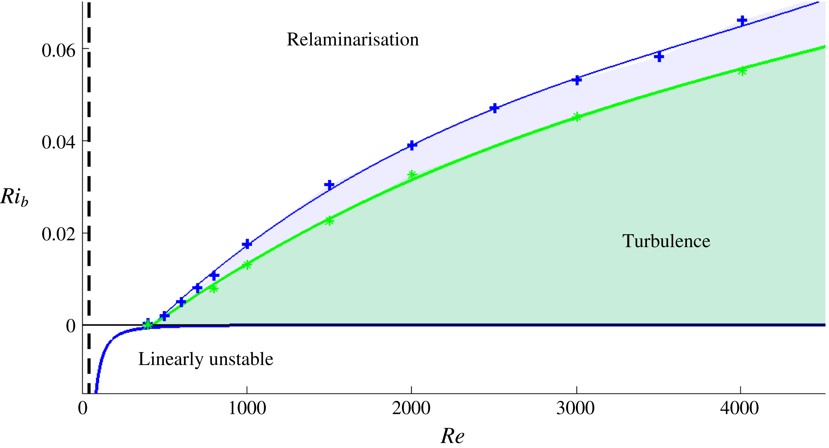
Laminar–turbulent boundary for two geometries
 $2\unicode[STIX]{x03C0}\times 2\times 2\unicode[STIX]{x03C0}$
(blue line through the crosses) and
 $2\unicode[STIX]{x03C0}\times 2\times \unicode[STIX]{x03C0}$
(green line through the stars). There is linear instability for
 $Ri_{b}<-1708/(16Re^{2}Pr)$
, which is the well-known Rayleigh–Bénard threshold (unchanged by shear – Kelly Reference Kelly and Spaulding1977). The energy stability limit is also marked as an (almost) vertical black dashed line.

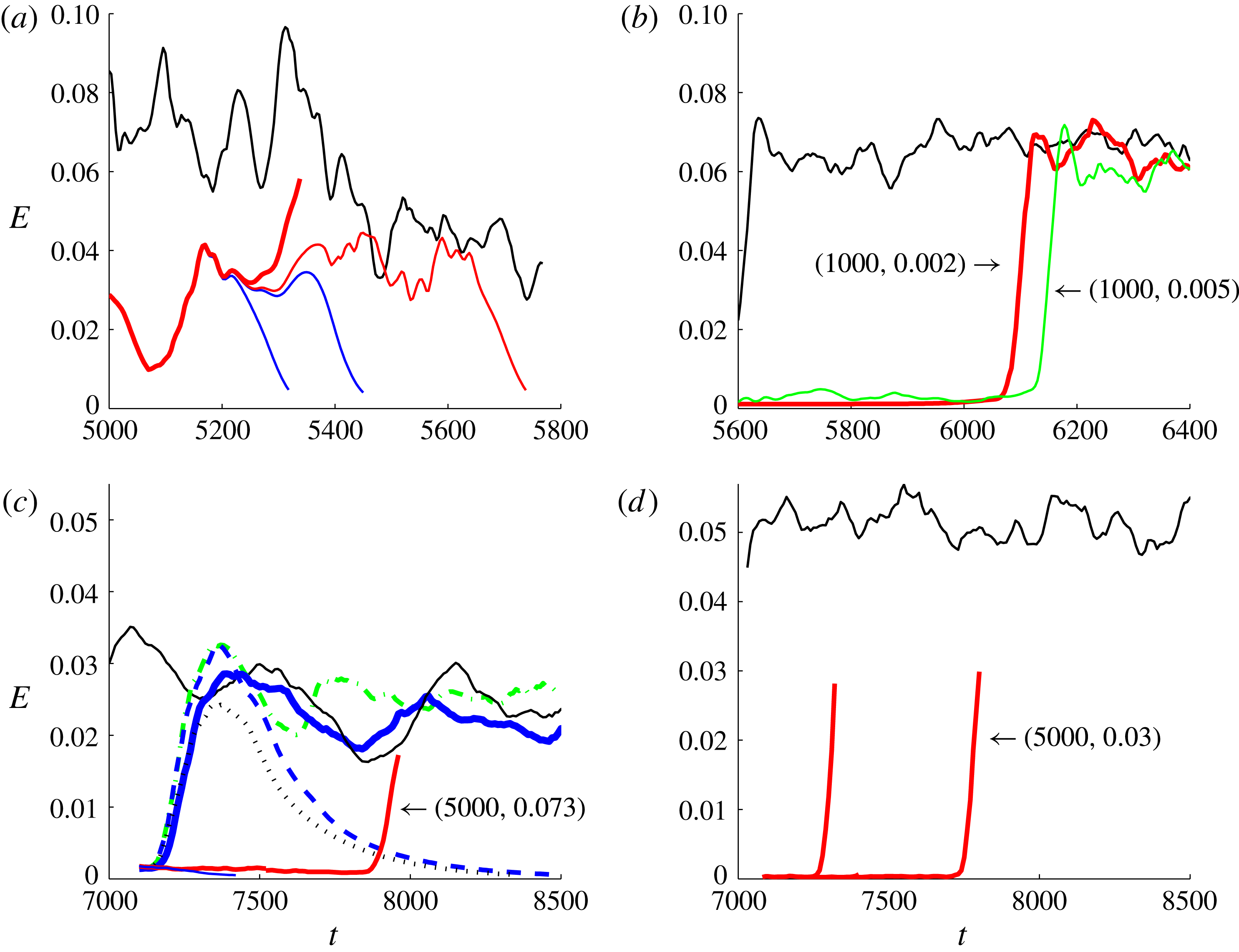
Edge (red, lower, flatter lines) and turbulent (black, upper, jagged lines) kinetic energy levels either receding from the laminar–turbulent boundary at fixed low
 $Ri_{b}$
and
 $Re$
increasing left to right (a,b) or from fixed
 $Re$
and
 $Ri_{b}$
decreasing left to right (c,d) (i.e. (a,c) are approaching the laminar–turbulent interface compared to (b,d)). (a)
 $(Re,Ri_{b})=(400,0.002)$
; (b)
 $(Re,Ri_{b})=(1000,0.002)$
red or
 $(Re,Ri_{b})=(1000,0.005)$
green; (c)
 $Re=5000$
and
 $Ri_{b}=0.073$
black,
 $Ri_{b}=0.075$
green dash–dot,
 $Ri_{b}=0.077$
blue dashed,
 $Ri_{b}=0.08$
blue or
 $Ri_{b}=0.085$
black dotted line; (d)
 $(Re,Ri_{b})=(5000,0.03)$
.

3 Results
3.1 Laminar–turbulent boundary
To set the scene for this investigation, we first choose some specific geometries and identify the laminar–turbulent boundary in
 $Re{-}Ri_{b}{-}Pr$
parameter space. In this paper
 $Pr=1$
throughout to keep this study focused, although dependency on
 $Pr$
across the range
 $0.7$
(heated air) through
 $7$
(heated water) to
 $700$
(salt in water) is an interesting issue for future examination. A simple protocol was adopted to estimate the position of the laminar–turbulent boundary for the two geometries
 $2\unicode[STIX]{x03C0}\times 2\times 2\unicode[STIX]{x03C0}$
and
 $2\unicode[STIX]{x03C0}\times 2\times \unicode[STIX]{x03C0}$
and for
 $Re\leqslant 5000$
. At a given point in the parameter plane
 $(Re{-}Ri_{b},1)$
, 10 simulations were performed with random initial conditions, with the point assigned to the turbulent region if
 $50\,\%$
or more of these runs remained turbulent after a time
 $1000\,h/U$
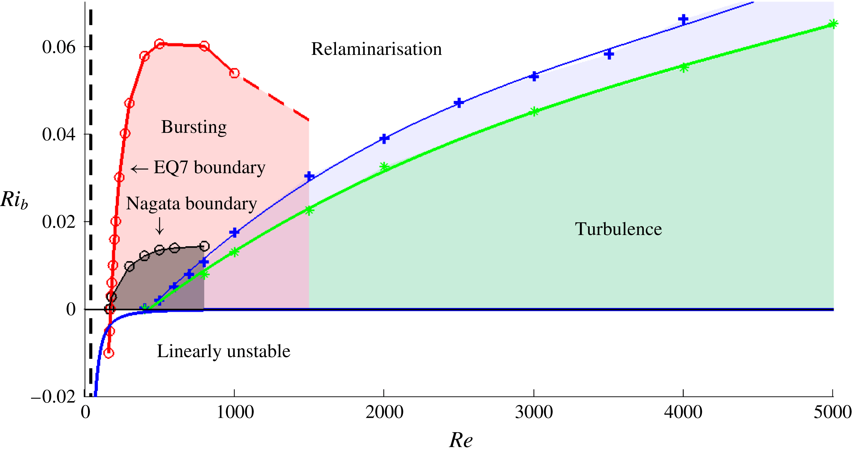
and otherwise assigned to the relaminarisation region. Figure 1 shows that the turbulent part of parameter space extends to higher
 $Ri_{b}$
at a given
 $Re$
for the larger domain with the boundary extending as
 $Re\rightarrow \infty$
for some
 $Ri_{b}(Re)$
(see Deusebio et al. (Reference Deusebio, Caulfield and Taylor2015) for a similar plot but at higher
 $Re$
and with larger domain size). Also shown for completeness is the region
 $Ri_{b}<0$
(unstable stratification), where the problem is equivalent to Rayleigh–Bénard convection with imposed shear: see appendix B which shows how the usual Rayleigh number
 $Ra=-Ri_{b}Re^{2}Pr$
and the neutral stability line is given by
 $Ra=1708/16$
(the extra factor of
 $16$
is present because the boundary separation has been non-dimensionalised to 2 rather than 1).
Since the laminar–turbulent boundary exists in a two-dimensional parameter plane, it can be approached in two different ways starting from the turbulent region: either decreasing
 $Re$
at fixed
 $Ri_{b}$
or increasing
 $Ri_{b}$
at fixed
 $Re$
. Work in unstratified flows indicates that the laminar–turbulent boundary (or ‘edge’ manifold if the turbulence is not strictly an attractor – see Skufca et al.
Reference Skufca, Yorke and Eckhardt2006) and the turbulent attractor collide when turbulence ceases to exist (e.g. figure 5 of Schneider & Eckhardt Reference Schneider and Eckhardt2009). This type of behaviour carries over to weakly stratified (small
 $Ri_{b}$
) shear flow here: the top plots in figure 2 show the energy levels of the turbulence and edge manifold coming together as
 $Re$
is decreased towards the boundary. A similar convergence of energy levels also seems to occur for fixed (high)
 $Re$
and increasing
 $Ri_{b}$
(figure 2
c,d), but the dominant feature now is the presence of increasingly large and slower fluctuations in the turbulent energy level as the boundary is approached. The lines for
 $Ri_{b}=0.077$
(blue dashed) and
 $Ri_{b}=0.08$
(solid blue) in figure 2(d) show how a less stratified flow can reach the energy levels of the turbulent state yet immediately relaminarise, while a more stratified flow can stay turbulent albeit with large fluctuations in energy. It seems that sustained turbulence is lost in the latter case by the turbulent attractor expanding to touch the edge manifold as opposed to moving as a whole towards it in the former case.
3.2 Identifying ECS: edge tracking
The method of edge tracking was used to identify ECS (Itano & Toh Reference Itano and Toh2001; Skufca et al.
Reference Skufca, Yorke and Eckhardt2006) without any imposed symmetries unless explicitly stated. This method seeks to find attractors on the laminar–turbulent boundary by a bisection approach. The approach can be ‘hit or miss’ – the attractor may turn out to be chaotic rather than simple (i.e. an equilibrium, travelling wave or periodic state) – but does have the advantage that if an ECS is found then it is known to help organise the transition process and therefore be dynamically important. Crucially, the method also offers an unbiased approach to finding ECS in contrast to simply taking known ECS at
 $Ri_{b}=0$
and continuing them into the region
 $Ri_{b}>0$
. Since adding stable stratification to a shear flow introduces the additional phenomenon of internal gravity waves, it is possible that new forms of ECS could exist strictly for
 $Ri_{b}>0$
. These would have different underpinning dynamics to that in unstratified flows (known variously as the self-sustaining process (SSP) – Waleffe (Reference Waleffe1995, Reference Waleffe1997) or vortex wave interaction (VWI) – Hall & Smith (Reference Hall and Smith1991), Hall & Sherwin (Reference Hall and Sherwin2010)) and therefore would be of considerable interest.
The investigation was started by reproducing Schneider et al.’s (Reference Schneider, Gibson, Lagher, De Lillo and Eckhardt2008) unstratified edge state calculation for
 $(Re,Ri_{b},L_{x},L_{z})=(400,0,4\unicode[STIX]{x03C0},2\unicode[STIX]{x03C0})$
. Adding even a little stratification (
 $Ri_{b}=1\times 10^{-3}$
) moved the system too close to the laminar–turbulent boundary to make edge tracking still feasible (the separation between the edge and the turbulent energy levels becomes too small), so
 $Re$
was increased to 1000. Here, the unstratified calculation recovers a variant of the edge state at
 $Re=400$
(a member of the Nagata (Reference Nagata1990) family of solutions), while taking
 $(Re,Ri_{b},L_{x},L_{z})=(1000,1\times 10^{-3},4\unicode[STIX]{x03C0},2\unicode[STIX]{x03C0})$
led to a spanwise-localised equilibrium with
 ${\mathcal{S}}$
and
 $\unicode[STIX]{x1D6FA}$
symmetries. Increasing
 $Ri_{b}$
above
 $1\times 10^{-3}$
led to a chaotic edge state, so the search was moved to a shorter domain
 $(Re,Ri_{b},L_{x},L_{z})=(1000,1\times 10^{-3},2\unicode[STIX]{x03C0},2\unicode[STIX]{x03C0})$
where edge tracking again revealed a spanwise-localised equilibrium. Branch-continuing this state back to the
 $4\unicode[STIX]{x03C0}\times 2\times 2\unicode[STIX]{x03C0}$
box recovered the spanwise-localised state found previously. Continuing this state in the
 $2\unicode[STIX]{x03C0}\times 2\times 2\unicode[STIX]{x03C0}$
box from
 $Ri_{b}=1\times 10^{-3}$
down to 0 and then continuing
 $Re$
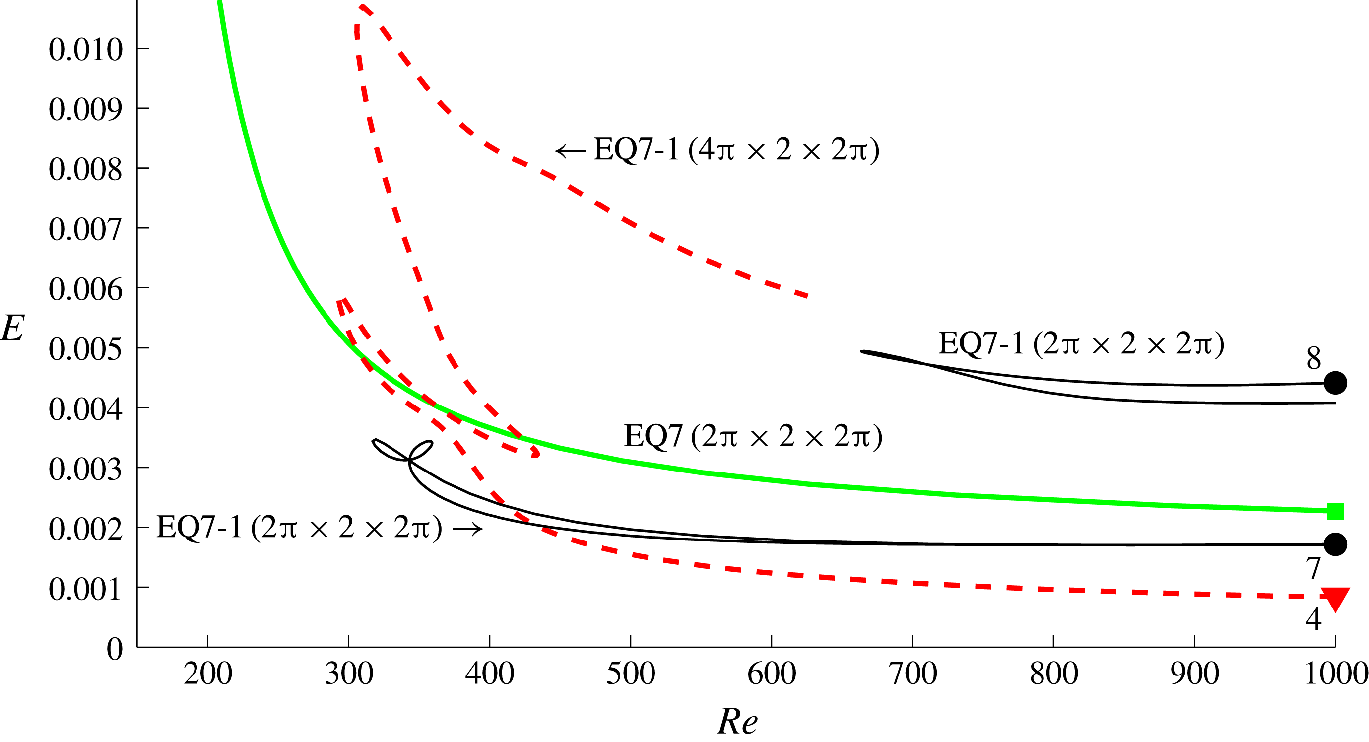
similarly downwards indicated that this spanwise-localised state was the stratified version of EQ7-1 in the nomenclature of Gibson & Brand (Reference Gibson and Brand2014): compare figure 3 with figure 4 of Gibson & Brand (Reference Gibson and Brand2014) (note that the ordinates are different and we have multiple curves for EQ7-1).
The results of continuing EQ7-1 around in
 $Ri_{b}$
at fixed
 $Re=1000$
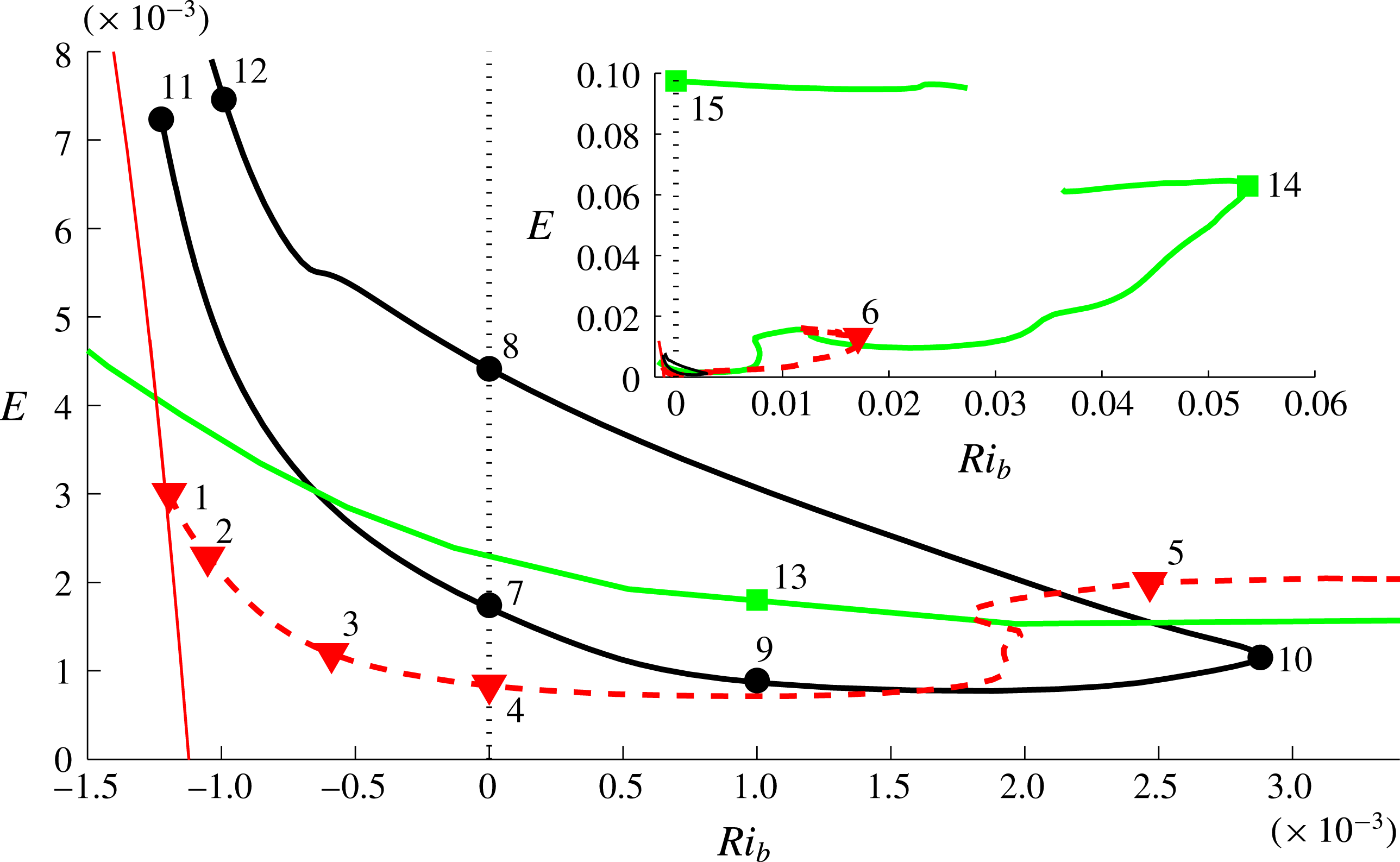
for both geometries are shown in figure 4. In the
 $4\unicode[STIX]{x03C0}\times 2\times 2\unicode[STIX]{x03C0}$
box, EQ7-1 exists at
 $Ri_{b}$
comparable to that at the laminar–turbulent boundary (see figure 1), whereas in the
 $2\unicode[STIX]{x03C0}\times 2\times 2\unicode[STIX]{x03C0}$
box, EQ7-1 only reaches to
 $Ri_{b}=2.87\times 10^{-3}$
before turning back. In the bigger box, figure 5 indicates that at the saddle node point (point of maximum
 $Ri_{b}$
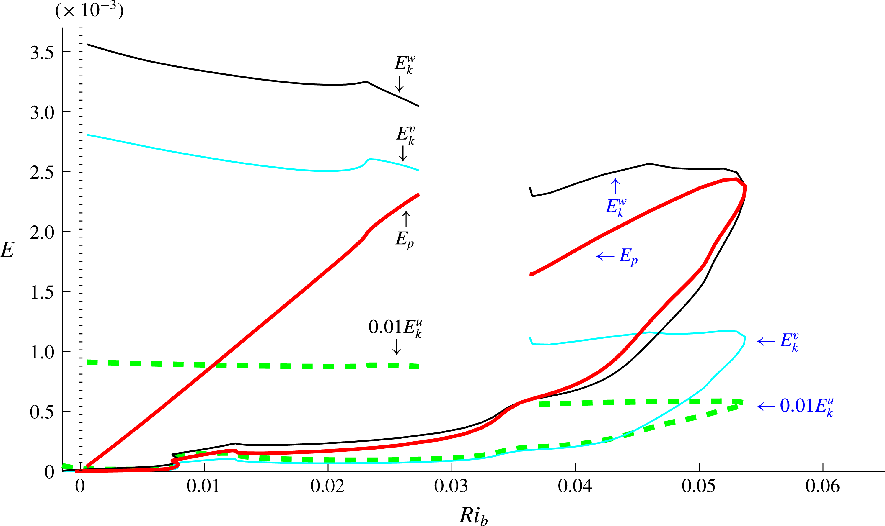
) the potential energy of EQ7-1 is almost twice the kinetic energy of the cross-stream (vertical) velocity. At this point the small streamwise rolls are being suppressed by the potential energy penalty imposed by the stable stratification: see § 3.4 for further discussion of this.
There is also a difference in continuing EQ7-1 between the two geometries at negative
 $Ri_{b}$
where the stratification is unstable: the
 $4\unicode[STIX]{x03C0}\times 2\times 2\unicode[STIX]{x03C0}$
EQ7-1 solutions connect to a 2-D solution branch of Rayleigh–Bénard rolls whereas the
 $2\unicode[STIX]{x03C0}\times 2\times 2\unicode[STIX]{x03C0}$
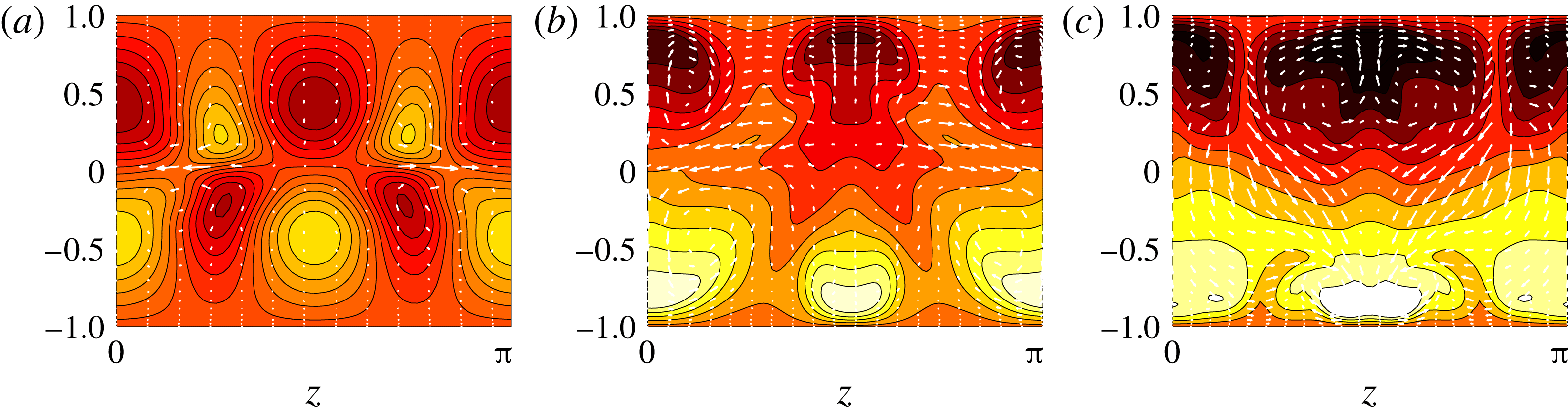
EQ7-1 solutions do not. Figures 6 and 7 indicate how the structure of EQ7-1 varies around these two solution branches. Figure 7 is particularly interesting as EQ7-1 starts out as spanwise global (top left and point 1 on the 2-D convective roll branch in figure 4) and then spanwise localises by point 4 (in figure 4). It achieves this by the flanks of the structure gradually ebbing away as
 $Ri_{b}$
is increased, which is made clear in figure 8. As discussed in § 4.1 of Gibson & Brand (Reference Gibson and Brand2014), this decay, at least at small amplitudes distant from the core of the flow structure, can be understood by identifying the least spatially damped steady eigenfunction of the linear operator based upon the basic state (typically this will be a 2-D eigenfunction invariant in the streamwise direction here). One consequence of this is the expectation that the rate of spatial evanescence increases as
 $Ri_{b}$
increases away from the bifurcation point where the decay rate is zero. Since the spanwise domain is relatively small, we do not attempt any further analysis here, but a similar process is observed when tracking a stratified version of the ‘snake’ solution of Schneider, Marinc & Eckhardt (Reference Schneider, Marinc and Eckhardt2010b
) and is analysed in Olvera & Kerswell (Reference Olvera and Kerswell2017).
Continuation in
 $Re$
at
 $Ri_{b}=0$
starting at
 $Re=1000$
for EQ7-1 in boxes
 $4\unicode[STIX]{x03C0}\times 2\times 2\unicode[STIX]{x03C0}$
(red dashed – – –) and
 $2\unicode[STIX]{x03C0}\times 2\times 2\unicode[STIX]{x03C0}$
(thin black —— for both, upper and lower disconnected branches), and continuation for EQ7 in box
 $2\unicode[STIX]{x03C0}\times 2\times \unicode[STIX]{x03C0}$
(bold green ——). Points 4, 7 and 8 are marked in the continuation in
 $Ri_{b}$
in figure 4.

Continuation in
 $Ri_{b}$
at
 $Re=1000$
for solution EQ7-1 in boxes
 $4\unicode[STIX]{x03C0}\times 2\times 2\unicode[STIX]{x03C0}$
(red dashed – – –) and
 $2\unicode[STIX]{x03C0}\times 2\times 2\unicode[STIX]{x03C0}$
(bold dark ——), EQ7 in box
 $2\unicode[STIX]{x03C0}\times 2\times \unicode[STIX]{x03C0}$
(bold green ——) and 2-D Rayleigh–Bénard solution in box
 $4\unicode[STIX]{x03C0}\times 2\times 2\unicode[STIX]{x03C0}$
(thin red ——). Inset shows how solution EQ7 reaches larger values of stratification close to
 $Ri_{b}\sim 0.06$
. The curves shown have been traced by continuing from the lower and upper branch solutions in the unstratified situation and cannot obviously be brought together – see § 3.3 for more details.

Continuation in
 $Ri_{b}$
at
 $Re=1000$
for solution EQ7-1 in box
 $4\unicode[STIX]{x03C0}\times 2\times 2\unicode[STIX]{x03C0}$
. Red dashed line in figure 4. The kinetic energy is split into its three components (
 $E_{u}$
,
 $E_{v}$
and
 $E_{w}$
).

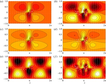
Contours of
 $y{-}z$
cross-sections of the streamwise component of the perturbation velocity
 $\hat{\boldsymbol{u}}$
(arrows indicate velocity field of
 $\hat{\boldsymbol{v}}$
–
 $\hat{\boldsymbol{w}}$
plane) of steady solution EQ7-1 at
 $Re=1000$
in box
 $2\unicode[STIX]{x03C0}\times 2\times 2\unicode[STIX]{x03C0}$
shown as black circles in figure 4: (a) pt 7 at
 $Ri_{b}=0$
; (b) pt 8 at
 $Ri_{b}=0$
; (c) pt 9 at
 $Ri_{b}=1\times 10^{-3}$
; (d) pt 10 at
 $Ri_{b}=2.88\times 10^{-3}$
; (e) pt 11 at
 $Ri_{b}=-1.22\times 10^{-3}$
; (f) pt 12 at
 $Ri_{b}=-9.9\times 10^{-4}$
. All plots have 8 contours between [
 $-$
0.31, 0.31], which are the minimum and maximum of the most energetic state at pt 11 (arrows rescaled as well).

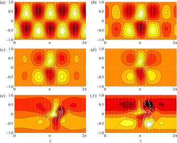
Contours of
 $y{-}z$
cross-sections of the streamwise component of the perturbation velocity
 $\hat{\boldsymbol{u}}$
(arrows indicate velocity field of
 $(\hat{\boldsymbol{v}},\hat{\boldsymbol{w}})$
plane) of steady solution EQ7-1 at
 $Re=1000$
in box
 $4\unicode[STIX]{x03C0}\times 2\times 2\unicode[STIX]{x03C0}$
shown as red triangles in figure 4: (a) pt 1; (b) pt 2; (c) pt 3; (d) pt 4; (e) pt 5; (f) pt 6. All plots have 8 contours between [
 $-0.48$
, 0.48], which are the minimum and maximum of the state at pt 7 (arrows rescaled as well).

Further edge tracking was done in a domain where the width was halved – so
 $(Re,Ri_{b},L_{x},L_{z})=(1000,1\times 10^{-3},2\unicode[STIX]{x03C0},\unicode[STIX]{x03C0})$
– which led to a global steady mode: see figure 9. This solution, which possesses all three symmetries
 ${\mathcal{S}},\unicode[STIX]{x1D6FA}$
and
 ${\mathcal{Z}}$
, is the stratified version of the hairpin vortex solution of Itano & Generalis (Reference Itano and Generalis2009), EQ7 in the nomenclature of Gibson, Halcrow & Cvitanović (Reference Gibson, Halcrow and Cvitanović2009) and the mirror-symmetric solution of Deguchi & Hall (Reference Deguchi and Hall2014, Reference Deguchi and Hall2015): hereafter we will refer to it as EQ7. The unstratified version has also been found before by edge tracking at the parameter settings
 $(Re,Ri_{b},L_{x},L_{z})=(1000,0,4.35\unicode[STIX]{x03C0},1.05\unicode[STIX]{x03C0})$
(see figure 5 of Rabin, Caulfield & Kerswell Reference Rabin, Caulfield and Kerswell2012). Figure 4 shows that EQ7 exists significantly above the laminar–turbulent boundary: figure 1 indicates that
 $Ri_{b}\approx 0.015$
at the boundary for the
 $2\unicode[STIX]{x03C0}\times 2\times \unicode[STIX]{x03C0}$
box whereas EQ7 extends up to
 $Ri_{b}\approx 0.055$
. As observed for EQ7-1, the solution branch for EQ7 turns back to lower
 $Ri_{b}$
when the potential energy of the state becomes approximately twice the kinetic energy in the cross-stream (vertical) direction: see figure 10. The EQ7 solution branch shown also could not be closed, which is investigated in § 3.3.
In the hunt for further ECS, edge tracking was also performed in small domains with various combinations of symmetries imposed and in extended (wider or longer) domains (typically with mirror symmetry
 ${\mathcal{Z}}$
imposed). However, only chaotic states were found beyond the ECS already identified. For example, edge tracking in the streamwise-extended domain
 $(Re,Ri_{b},L_{x},L_{z})=(1000,1\times 10^{-3},16\unicode[STIX]{x03C0},2\unicode[STIX]{x03C0})$
, with and without
 ${\mathcal{Z}}$
-symmetry imposed, led to streamwise-localised chaotic states as in Schneider et al. (Reference Schneider, Marinc and Eckhardt2010b
). Some computations were also done for strong stratification (
 $Ri_{b}=0.1$
) and
 $Re=10\,000$
in small domains, but again only chaotic edge states were found even in really small domains like
 $\unicode[STIX]{x03C0}\times 2\times \textstyle \frac{1}{4}\unicode[STIX]{x03C0}$
constrained by the imposition of the mirror symmetry
 ${\mathcal{Z}}$
.
Since both EQ7-1 and EQ7 could be continued back to the unstratified limit,
 $Ri_{b}=0$
(see figure 4), and looked to have all the features associated with SSP/VWI (dominant streaks with secondary streamwise rolls and wave field), no purely stratified ECS (ECS with no
 $Ri_{b}=0$
limit) were found. Such new ECS probably only exist at much larger
 $Ri_{b}$
than that found for
 $Re=O(5000)$
since the ratio of internal gravity wave time scale to advective time scale (
 $h/U$
) is
 $1/\sqrt{Ri_{b}}$
. This presumably needs to be
 $O(1)$
to be important, which, as we argue below, only occurs at large
 $Re$
when the ECS becomes fully localised. The fact that EQ7 exists beyond the laminar–turbulent boundary for the
 $Re$
examined (
 $Re\leqslant 1000$
– see figure 11) at least confirms the general consensus that ECS are a necessary precursor (now as
 $Ri_{b}$
decreases at fixed
 $Re$
) for turbulence to be possible. In fact, the region where EQ7 exists but turbulence does not possesses a ‘bursting’ phenomenon – see figure 11 – where certain initial conditions can give rise to large energy growth up to energy levels commensurate with the turbulent state at lower
 $Ri_{b}$
(see Olvera & Kerswell (Reference Olvera and Kerswell2017) for more details). Henceforth we focus on studying EQ7. Before considering the question of how large
 $Ri_{b}$
can become and still have ECS, we first examine the stratification of Nagata’s (Reference Nagata1990) first solution and how it relates to EQ7.
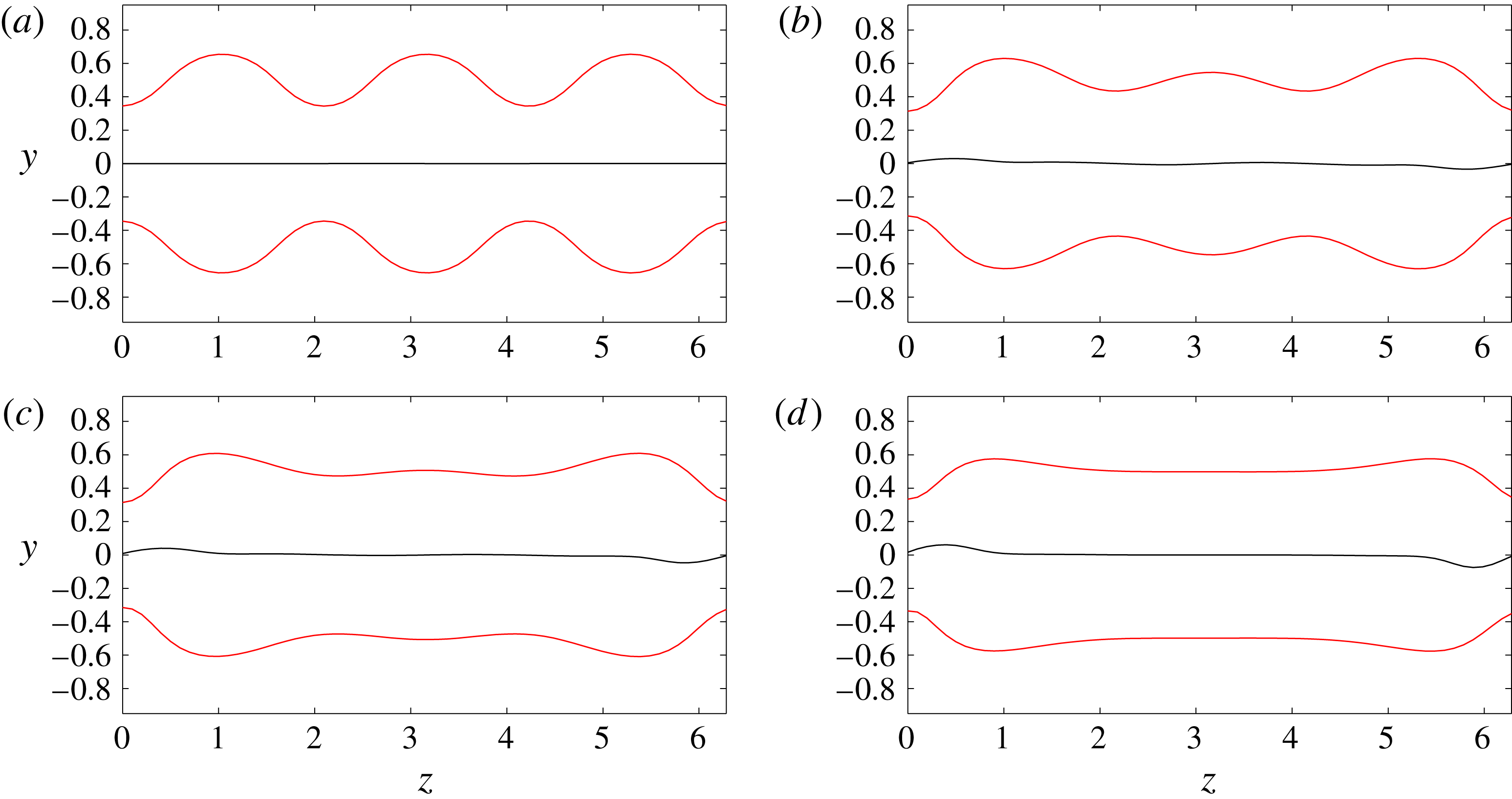
Contours of total velocity
 $\boldsymbol{u}$
at levels
 $\boldsymbol{u}=\{0,\pm 0.05\}$
of steady solution EQ7-1 at
 $Re=1000$
in box
 $4\unicode[STIX]{x03C0}\times 2\times 2\unicode[STIX]{x03C0}$
shown as red triangles in figure 4: (a) pt 1; (b) pt 2; (c) pt 3; (d) pt 4. All states have been shifted in the spanwise direction by half the domain to highlight the gradual evanescence of the central domain.

Contours of
 $y{-}z$
cross-sections of streamwise component of perturbation velocity
 $\hat{\boldsymbol{u}}$
(arrows indicate velocity field of
 $\hat{\boldsymbol{v}}$
–
 $\hat{\boldsymbol{w}}$
plane) of steady solution EQ7 at
 $Re=1000$
in box
 $2\unicode[STIX]{x03C0}\times 2\times \unicode[STIX]{x03C0}$
shown as squares in figure 4: (a) pt 13 at
 $Ri_{b}=0.001$
; (b) pt 14 at
 $Ri_{b}=0.053$
; (c) pt 15 at
 $Ri_{b}=0$
upper branch. All plots have 8 contours between [
 $-$
1.02, 0.83], which are the minimum and maximum of the state at pt 13 (arrows rescaled as well).

Continuation in
 $Ri_{b}$
at
 $Re=1000$
for solution EQ7 in box
 $2\unicode[STIX]{x03C0}\times 2\times \unicode[STIX]{x03C0}$
(see inset of figure 4). The kinetic energy is split into its three components (
 $E_{u}$
,
 $E_{v}$
and
 $E_{w}$
).

Parameter space (with
 $Pr=1$
): the
 $Re{-}Ri_{b}$
plane. The blue line indicates the turbulent–laminar boundary for box
 $2\unicode[STIX]{x03C0}\times 2\times 2\unicode[STIX]{x03C0}$
and the green line for box
 $2\unicode[STIX]{x03C0}\times 2\times \unicode[STIX]{x03C0}$
. The red line shows the area of existence for EQ7 and its likely continuation is discussed in § 3.4.

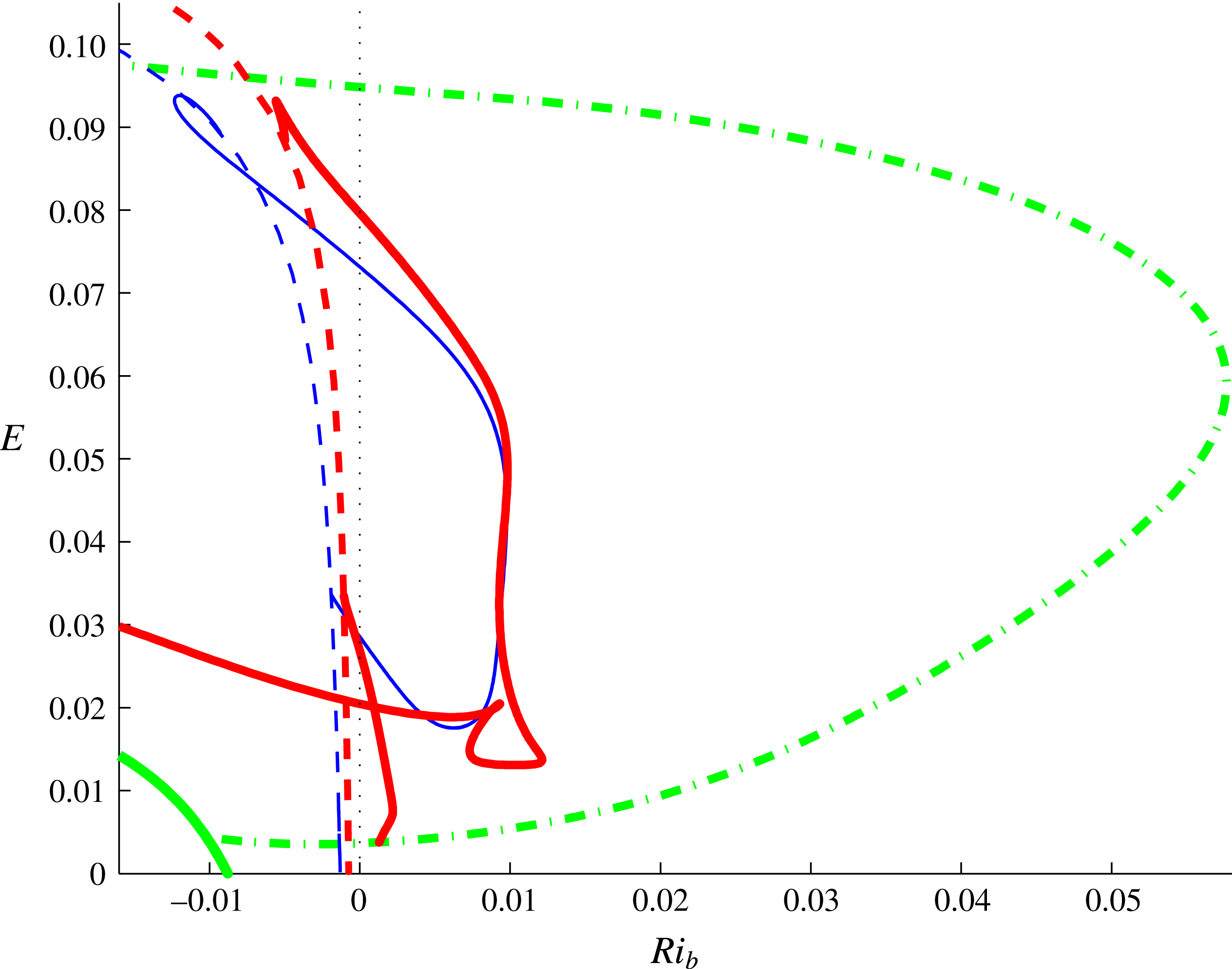
Energy
 $E$
versus
 $Ri_{b}$
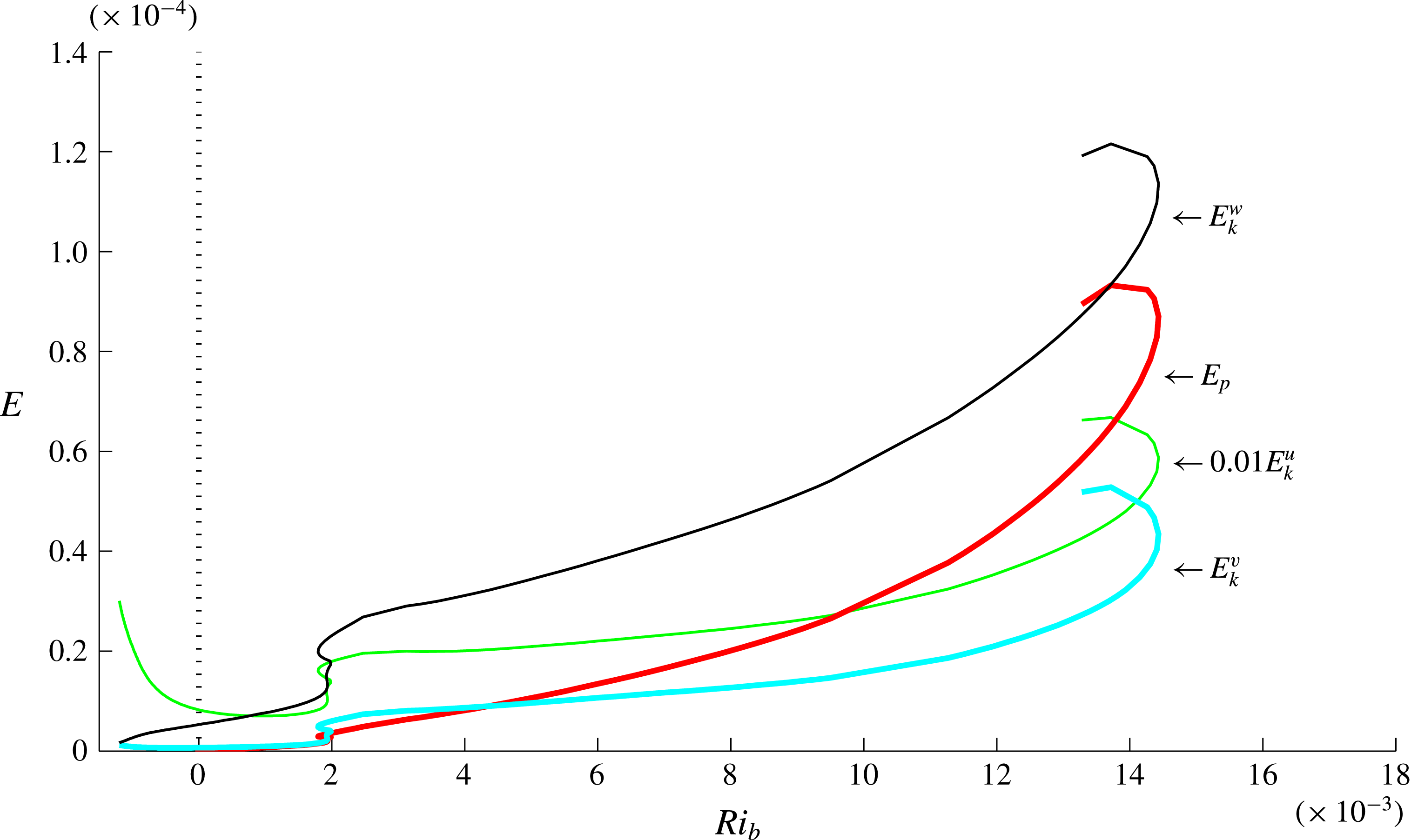
for Nagata solution at
 $Re=300$
(thin solid blue line) and
 $Re=400$
(thick solid red line) together with EQ7 at
 $Re=400$
(green dash-dot line) and 2-D convective roll solutions (thin and thick dashed lines and the very thick line in the bottom left corner) for
 $Ri_{b}<0$
. The plot shows that Nagata solution branch is initially (at
 $Re=300$
) a loop which starts and finishes on a 2-D convective roll branch whereas, at
 $Re=400$
, this loop has broken to connect to the EQ7 solution branch. The upper Nagata solution branch arm then extends back to convectively unstable flows.

3.3 EQ7 and Nagata’s solution
Nagata’s (Reference Nagata1990) solution was the first finite-amplitude state discovered in plane Couette flow and it has been known since the work of Clever & Busse (Reference Clever and Busse1992) that this solution actually bifurcates off a 2-D (single layer) roll solution in Rayleigh–Bénard convection (negative
 $Ri_{b}$
). It has been found here that EQ7 also bifurcates off a 2-D (double layer) roll solution – see figure 12. Since Nagata’s solution has one less symmetry than EQ7, one could expect that Nagata’s solution bifurcates off EQ7 in a symmetry-breaking bifurcation. This is indeed the case at least at
 $Re=400$
: see figure 12 which also shows that
 $Ri_{b}$
does not need to be increased very far before Nagata’s solution ceases to exist compared to EQ7. Figure 11 further emphasises this.
Before considering EQ7 at large
 $Re$
, we first return to an issue shown in figure 4. The inset of figure 4 shows two continuations of EQ7 at
 $Re=1000$
in a box
 $2\unicode[STIX]{x03C0}\times 2\times \unicode[STIX]{x03C0}$
, one starting at the edge-tracked solution at
 $Ri_{b}=1\times 10^{-3}$
(the lower branch) and the other starting from the upper branch solution at
 $Ri_{b}=0$
(obtained by continuing the lower branch solution back to
 $Ri_{b}=0$
and then continuing around the saddle node using the spanwise wavenumber). At lower
 $Re$
, these two continuations meet (e.g. at
 $Re=400$
as shown in figure 12) when varying
 $Ri_{b}$
to produce a smooth connection between unstratified upper and lower branch solutions, but they clearly do not at
 $Re=1000$
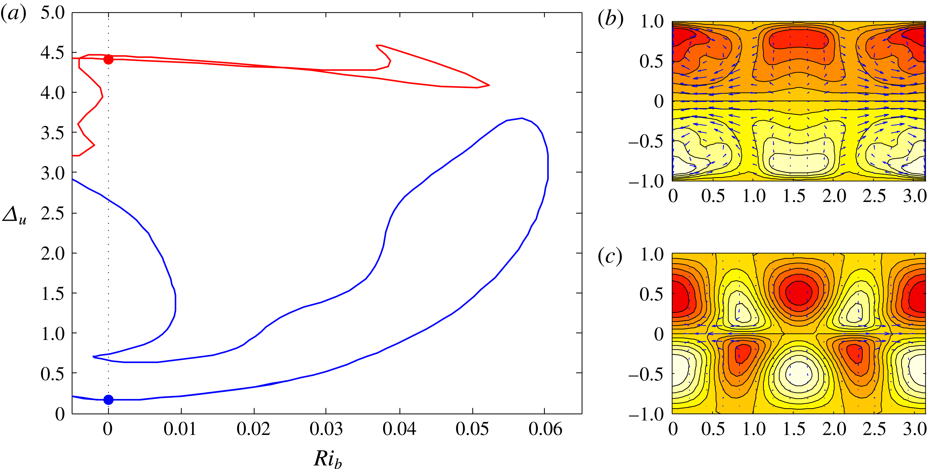
. At
 $Re=500$
– see figure 13 – the connection between upper and lower unstratified solutions has broken. Tracing the new crossings of the
 $Ri_{b}=0$
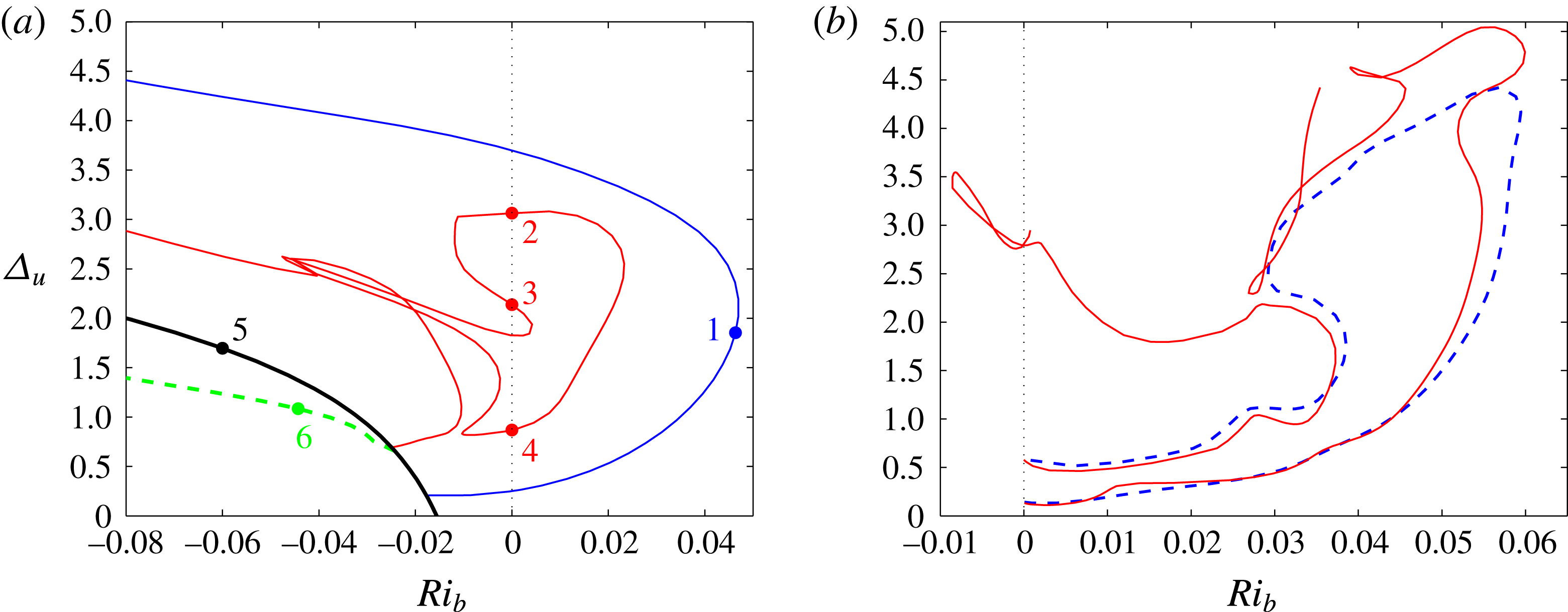
line reveals what looks to be a previously unknown branch of ‘inner’ solutions, coloured red in figure 14(a) at
 $Re=300$
, which bifurcates off a 3-D state and almost immediately after that bifurcates off a double roll state in Rayleigh–Bénard convection (
 $Ri_{b}<0$
). A further lower branch breakup occurs between
 $Re=700$
and
 $Re=850$
as shown in figure 14(b), which finally explains the complicated continuation curve at
 $Re=1000$
in the inset of figure 4. Clearly, stable stratification has a strong influence on the states. We now turn our attention to understanding exactly why.
Continuation in
 $Ri_{b}$
of EQ7 at
 $Re=500$
in a box
 $2\unicode[STIX]{x03C0}\times 2\times \unicode[STIX]{x03C0}$
. Dots on the
 $Ri_{b}=0$
axis indicate known upper and lower unstratified solutions. Panel (b) shows the state (contours of
 $\hat{u}$
and arrows for
 $(\hat{v},{\hat{w}})$
) at the upper (red) dot (12 contour levels across [
 $-1.02,1.02$
]) and panel (c) shows the state at the lower (blue) dot (12 contour levels across [
 $-0.17$
, 0.17]).

(a) EQ7 continuation in
 $Ri_{b}$
at
 $Re=300$
in a box
 $2\unicode[STIX]{x03C0}\times 2\times \unicode[STIX]{x03C0}$
. The inner (red) branch connects to the dashed green 3-D branch of
 $x$
-wavelength
 $\unicode[STIX]{x03C0}$
just after it itself bifurcates off the black 2-D roll branch. The outer (blue) branch bifurcates directly off the black 2-D roll branch. Typical resolution used
 $(M,N,L)=(16,25,16)$
and plots of the various states marked by dots and numbers are given in figure 15. (b) Lower branch continuation for EQ7 in
 $Ri_{b}$
at
 $Re=700$
(blue dashed line) in a box
 $2\unicode[STIX]{x03C0}\times 2\times \unicode[STIX]{x03C0}$
which is comparable with that at
 $Re=500$
and
 $Re=850$
(red solid line). This plot shows that the lower branch loop at
 $Re=700$
has broken up into two disconnected pieces at
 $Re=850$
(this breakup happens in the interval
 $(800,850)$
). Typical resolutions used to confirm this behaviour were
 $(M,N,L)=(12,25,16)$
,
 $(14,40,20)$
and
 $(16,30,20)$
.

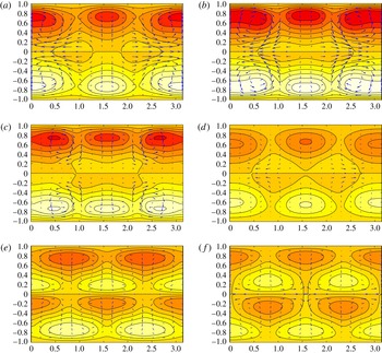
EQ7 flow states (contours of
 $\hat{u}$
and arrows for
 $(\hat{v},{\hat{w}})$
) shown over a
 $y{-}z$
plane at
 $Re=300$
: (a) state 1 shown in figure 14, (b) state 2, (c) state 3, (d) state 4, (e) state 5 and (f) state 6. There are 12 contours over [
 $-0.725,0.725$
] (red–white) and maximum cross-flow speed is 0.296 across all plots to show the relative strengths of the states.

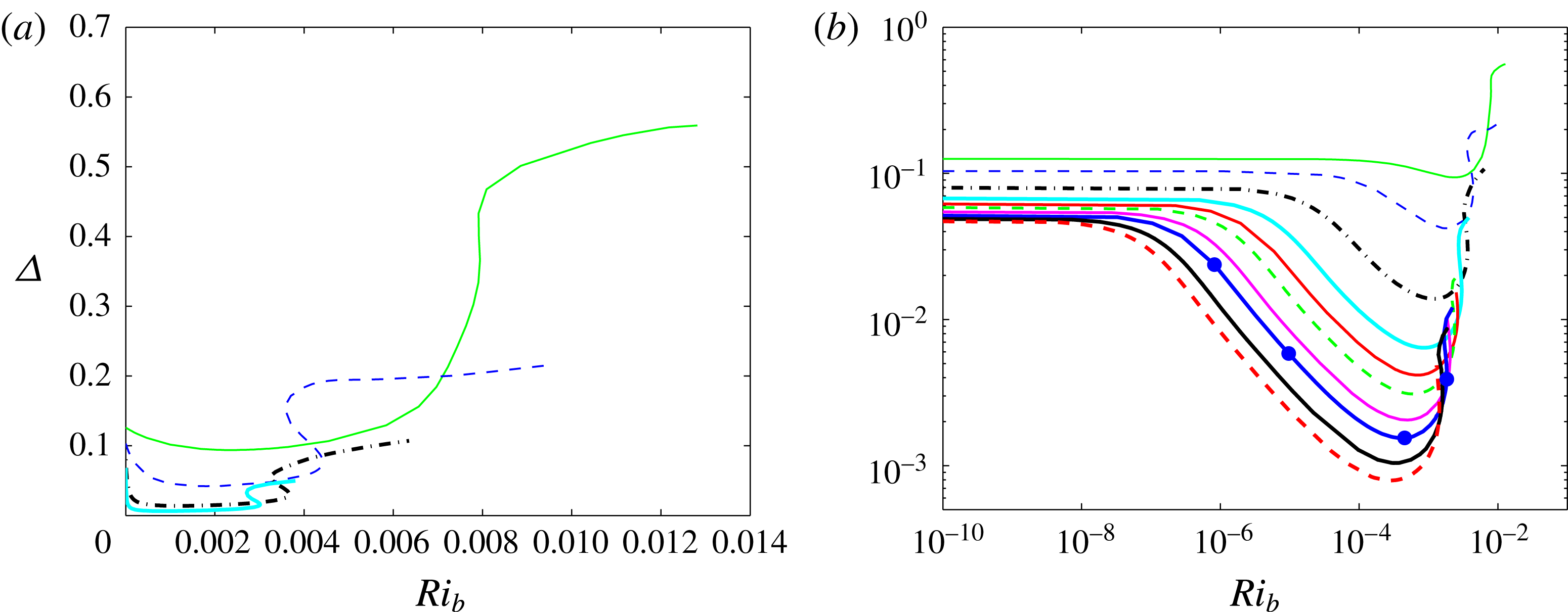
(a) The wall shear stress deviation
 $\unicode[STIX]{x1D6E5}$
as a function of
 $Ri_{b}$
for the lower branch of EQ7 at
 $Re=1000$
(green solid),
 $2000$
(blue dashed),
 $5000$
(black thick dash-dot) and
 $10\,000$
(cyan thick solid). All curves show an initial drop in stress from the unstratified value, a minimum of stress at some finite
 $Ri_{b}^{min}$
and two turning points where the curve reaches a local maximum in
 $Ri_{b}^{max}$
and then a local minimum in
 $Ri_{b}$
. (b) The same data as in (a) but plotted on a log–log scale with extra lower branch data (at
 $15\,000$
(red solid),
 $20\,000$
(green dashed),
 $30\,000$
(magenta solid),
 $40\,000$
(blue thick solid),
 $60\,000$
(black thick solid) and
 $80\,000$
(red thick dashed)) added. The velocity states corresponding to the four blue dots on the blue
 $Re=40\,000$
curve – at
 $Ri_{b}\approx 10^{-6}$
,
 $10^{-5}$
, the minimum stress point
 $Ri_{b}^{min}=4.15\times 10^{-4}$
and the local maximum point
 $Ri_{b}^{max}=1.833\times 10^{-3}$
– are shown in figure 17.

EQ7 flow states (contours of
 $\hat{u}$
and arrows for
 $(\hat{v},{\hat{w}})$
) shown over a
 $y{-}z$
plane at
 $Re=40\,000$
. The states correspond to the blue dots in figure 16(b) with the order (a), (b), (c) (the stress minimum), (d) corresponding to increasing
 $Ri_{b}$
. The contour levels for the streamwise velocity perturbation
 $\hat{u} =u-y$
(the arrows indicate
 $v\hat{\boldsymbol{y}}+w\hat{\boldsymbol{z}}$
) are as follows: (a) 10 contours between
 $\pm 6.73\times 10^{-2}$
(arrow max.
 $1.0\times 10^{-3}$
); (b) 10 contours between
 $\pm 3.8\times 10^{-2}$
(arrow max.
 $1.1\times 10^{-3}$
); (c) 10 contours between
 $\pm 1.81\times 10^{-2}$
(arrow max.
 $1.8\times 10^{-3}$
); and (d) 10 contours between
 $\pm 2.31\times 10^{-2}$
(arrow max.
 $2.51\times 10^{-3}$
). The dashed black lines on each plot correspond to the
 $y$
level of the corresponding
 $x$
–
 $z$
slices shown in figure 18.

EQ7 flow states shown over a
 $x-z$
plane at
 $Re=40\,000$
and the
 $y$
levels shown in figure 17 (
 $y=0.2$
,
 $0.13$
,
 $0.07$
and
 $0.05$
respectively). The contour levels for the streamwise velocity perturbation
 $u-y$
are as follows: (a) 10 contours across
 $[-0.042,0.061]$
; (b) 10 contours across
 $[-0.0142,0.033]$
; (c) 10 contours across
 $[-0.00669,0.0166]$
; and (d) 10 contours across
 $[-0.0216,0.0239]$
.

The density perturbation
 $\unicode[STIX]{x1D70C}+y$
for the third and fourth EQ7 flow states shown in figures 17 and 18 over a
 $x-z$
plane at
 $y=0.07$
(a) and
 $0.05$
(b). The contour levels are as follows: (a), 10 contours across
 $[-0.0167,0.00692]$
; and (b), 10 contours across
 $[-0.024,0.022]$
.

3.4 EQ7 asymptotics
To gain some understanding of how stratification affects the SSP/VWI states at large
 $Re$
, we concentrate on understanding how the lower branch EQ7 solutions behave as
 $Ri_{b}$
is increased from 0 at large
 $Re$
. Of particular interest is how the maximum Richardson number for such states scales with
 $Re$
. Figure 16 shows how the wall shear stress deviation
 $\unicode[STIX]{x1D6E5}$
varies as
 $Ri_{b}$
increases for the lower branch of EQ7. All curves show an initial drop in stress from the unstratified value, a minimum of stress at some finite
 $Ri_{b}^{min}$
and then two turning points where the curve reaches a local maximum in
 $Ri_{b}:=Ri_{b}^{max}$
and then a local minimum in
 $Ri_{b}$
. Four states at
 $Re=40\,000$
and various values of
 $Ri_{b}$
(marked by blue dots in figure 16) are shown in figure 17, which indicates that EQ7 transitions from a global flow state to one showing localisation in the cross-shear direction
 $y$
and further localisation in the spanwise direction
 $z$
. The first two states, which appear global, can be described as being in regime 1, whereas the second two states, which are clearly localised, indicate a second and possibly third regime.
3.4.1 Regime 1
Regime 1 corresponds to the range of
 $Ri_{b}$
where a stratified version of the VWI structure of Hall & Sherwin (Reference Hall and Sherwin2010) is realised. The only prior work to consider stratification is Hall (Reference Hall2012), which looked at the natural convection situation where the stratification is parallel to the shear: differences from our case here of stratification perpendicular to the shear will be highlighted below. A first key observation is that because EQ7 is steady and
 $\unicode[STIX]{x1D6FA}$
-symmetric, the critical layer
 $u=0$
is always located on
 $y=0$
and therefore has no curvature. To keep the discussion general, we broaden the direction of gravity
 $g$
to
 $-\cos \,\unicode[STIX]{x1D703}\hat{\boldsymbol{y}}-\sin \unicode[STIX]{x1D703}\hat{\boldsymbol{z}}$
and consider two cases:
 $\unicode[STIX]{x1D703}=0$
is ‘cross-stream’ gravity perpendicular to the boundaries, and
 $\unicode[STIX]{x1D703}=\unicode[STIX]{x03C0}/2$
is ‘spanwise’ gravity aligned with the boundaries; in the geophysical literature, these limiting cases are usually referred to as ‘vertical’ and ‘horizontal’ stratified shear situations respectively. The governing equations in component form for the total fields (recall from (2.7a,b
) that
 $\boldsymbol{u}=\hat{\boldsymbol{u}}+y\hat{\boldsymbol{x}}$
and
 $\unicode[STIX]{x1D70C}=\hat{\unicode[STIX]{x1D70C}}-y$
) are
 $$\begin{eqnarray}\displaystyle & \displaystyle u_{t}+uu_{x}+vu_{y}+wu_{z}+p_{x}={\displaystyle \frac{1}{Re}}\unicode[STIX]{x1D6FB}^{2}u, & \displaystyle\end{eqnarray}$$
 $$\begin{eqnarray}\displaystyle & \displaystyle v_{t}+uv_{x}+vv_{y}+wv_{z}+p_{y}={\displaystyle \frac{1}{Re}}\unicode[STIX]{x1D6FB}^{2}v-Ri_{b}\;\unicode[STIX]{x1D70C}\cos \unicode[STIX]{x1D703}, & \displaystyle\end{eqnarray}$$
 $$\begin{eqnarray}\displaystyle & \displaystyle w_{t}+uw_{x}+vw_{y}+ww_{z}+p_{z}={\displaystyle \frac{1}{Re}}\unicode[STIX]{x1D6FB}^{2}w-Ri_{b}\;\unicode[STIX]{x1D70C}\sin \unicode[STIX]{x1D703}, & \displaystyle\end{eqnarray}$$
 $$\begin{eqnarray}\displaystyle & \displaystyle \unicode[STIX]{x1D70C}_{t}+u\unicode[STIX]{x1D70C}_{x}+v\unicode[STIX]{x1D70C}_{y}+w\unicode[STIX]{x1D70C}_{z}={\displaystyle \frac{1}{Re\,Pr}}\unicode[STIX]{x1D6FB}^{2}\unicode[STIX]{x1D70C}, & \displaystyle\end{eqnarray}$$
 $$\begin{eqnarray}\displaystyle & \displaystyle u_{x}+v_{y}+w_{z}=0. & \displaystyle\end{eqnarray}$$
Note also that the effect of the transformations
 ${\mathcal{S}},\unicode[STIX]{x1D6FA}$
and
 ${\mathcal{Z}}$
detailed in (2.8), (2.9) and (2.10) is for the (original)
 $\unicode[STIX]{x1D703}=0$
case where the transformations experienced by
 $v$
and
 $\unicode[STIX]{x1D70C}$
match (for
 $\unicode[STIX]{x1D703}=\unicode[STIX]{x03C0}/2$
the transformation properties of
 $\unicode[STIX]{x1D70C}$
have to be changed to match those of
 $w$
and for general
 $\unicode[STIX]{x1D703}$
there are no such symmetries). Following Hall & Sherwin (Reference Hall and Sherwin2010), we look for steady solutions away from the critical layer of the form
 $$\begin{eqnarray}\displaystyle & \displaystyle u=\bar{u}(y,z)+\cdots +\unicode[STIX]{x1D6FF}Re^{-1/3}(U(y,z)\text{e}^{\text{i}\unicode[STIX]{x1D6FC}x}+\text{c.c})+\cdots \,, & \displaystyle\end{eqnarray}$$
 $$\begin{eqnarray}\displaystyle & \displaystyle v=Re^{-1}\bar{v}(y,z)+\cdots +\unicode[STIX]{x1D6FF}Re^{-1/3}(V(y,z)\text{e}^{\text{i}\unicode[STIX]{x1D6FC}x}+\text{c.c})+\cdots \,, & \displaystyle\end{eqnarray}$$
 $$\begin{eqnarray}\displaystyle & \displaystyle w=Re^{-1}\bar{w}(y,z)+\cdots +\unicode[STIX]{x1D6FF}Re^{-1/3}(W(y,z)\text{e}^{\text{i}\unicode[STIX]{x1D6FC}x}+\text{c.c})+\cdots \,, & \displaystyle\end{eqnarray}$$
 $$\begin{eqnarray}\displaystyle & \displaystyle \unicode[STIX]{x1D70C}=\bar{\unicode[STIX]{x1D70C}}(y,z)+\cdots +\unicode[STIX]{x1D6FF}Re^{-1/3}(R(y,z)\text{e}^{\text{i}\unicode[STIX]{x1D6FC}x}+\text{c.c})+\cdots \,, & \displaystyle\end{eqnarray}$$
 $$\begin{eqnarray}\displaystyle & \displaystyle p=Re^{-2}\bar{p}(y,z)+\cdots +\unicode[STIX]{x1D6FF}Re^{-1/3}(P(y,z)\text{e}^{\text{i}\unicode[STIX]{x1D6FC}x}+\text{c.c})+\cdots \,, & \displaystyle\end{eqnarray}$$
where c.c. denotes complex conjugate and all components of the wave field
 $(U,V,W,R,P)$
are assumed to be of equal magnitude, consistent with spatial scales being similar in every direction. The small parameter
 $Re^{-1/3}$
is the usual scaling for a critical layer where advection by the mean flow is balanced by viscous terms (e.g. see Hall & Sherwin Reference Hall and Sherwin2010), and
 $\unicode[STIX]{x1D6FF}$
is the wave amplitude in the critical layer to be determined later. Substituting these expansions into equations (3.1)–(3.4) gives, to leading order in
 $Re$
, for the
 $x$
-independent part (the roll and streak equations)
 $$\begin{eqnarray}\displaystyle & \displaystyle \bar{v}\bar{u}_{y}+\bar{w}\bar{u}_{z}=\bar{u}_{yy}+\bar{u}_{zz}, & \displaystyle\end{eqnarray}$$
 $$\begin{eqnarray}\displaystyle & \displaystyle \bar{v}\bar{v}_{y}+\bar{w}\bar{v}_{z}+\bar{p}_{y}=\bar{v}_{yy}+\bar{v}_{zz}-Re^{2}Ri_{b}\;\bar{\unicode[STIX]{x1D70C}}\cos \unicode[STIX]{x1D703}, & \displaystyle\end{eqnarray}$$
 $$\begin{eqnarray}\displaystyle & \displaystyle \bar{v}\bar{w}_{y}+\bar{w}\bar{w}_{z}+\bar{p}_{z}=\bar{w}_{yy}+\bar{w}_{zz}-Re^{2}Ri_{b}\;\bar{\unicode[STIX]{x1D70C}}\sin \unicode[STIX]{x1D703}, & \displaystyle\end{eqnarray}$$
 $$\begin{eqnarray}\displaystyle & \displaystyle \bar{v}\bar{\unicode[STIX]{x1D70C}}_{y}+\bar{w}\bar{\unicode[STIX]{x1D70C}}_{z}={\displaystyle \frac{1}{Pr}}(\bar{\unicode[STIX]{x1D70C}}_{yy}+\bar{\unicode[STIX]{x1D70C}}_{zz}), & \displaystyle\end{eqnarray}$$
 $$\begin{eqnarray}\displaystyle & \displaystyle \bar{v}_{y}+\bar{w}_{z}=0, & \displaystyle\end{eqnarray}$$
and for the
 $x$
-dependent (wave) part
 $$\begin{eqnarray}\displaystyle & \displaystyle \text{i}\unicode[STIX]{x1D6FC}\bar{u}U+V\bar{u}_{y}+W\bar{u}_{z}+\text{i}\unicode[STIX]{x1D6FC}P=0, & \displaystyle\end{eqnarray}$$
 $$\begin{eqnarray}\displaystyle & \displaystyle \text{i}\unicode[STIX]{x1D6FC}\bar{u}V+P_{y}=-Ri_{b}\;R\cos \unicode[STIX]{x1D703}, & \displaystyle\end{eqnarray}$$
 $$\begin{eqnarray}\displaystyle & \displaystyle \text{i}\unicode[STIX]{x1D6FC}\bar{u}W+P_{z}=-Ri_{b}\;R\sin \unicode[STIX]{x1D703}, & \displaystyle\end{eqnarray}$$
 $$\begin{eqnarray}\displaystyle & \displaystyle \text{i}\unicode[STIX]{x1D6FC}\bar{u}R+V\bar{\unicode[STIX]{x1D70C}}_{y}+W\bar{\unicode[STIX]{x1D70C}}_{z}=0, & \displaystyle\end{eqnarray}$$
 $$\begin{eqnarray}\displaystyle & \displaystyle \text{i}\unicode[STIX]{x1D6FC}U+V_{y}+W_{z}=0, & \displaystyle\end{eqnarray}$$
which are just the inviscid linearised Navier–Stokes equations about the streak field with critical layer at
 $\bar{u}(y,z)=0$
. In the
 $x$
-independent equations (3.11)–(3.15), the leading nonlinear terms due to the wave field are
 $O(\unicode[STIX]{x1D6FF}^{2}Re^{1/3})$
smaller in the
 $\bar{u}$
and
 $\bar{\unicode[STIX]{x1D70C}}$
equations and
 $O(\unicode[STIX]{x1D6FF}^{2}Re^{4/3})$
smaller in the
 $\bar{v}$
and
 $\bar{w}$
equations. Therefore, providing
 $\unicode[STIX]{x1D6FF}=o(Re^{-2/3})$
, the rolls and streaks are unforced in the interior and so, if they are not to slowly dissipate, must be forced by the critical layer through matching conditions across it – this is the essence of the VWI theory of Hall & Sherwin (Reference Hall and Sherwin2010). Also at this point it is clear that stratification first affects the roll equations when
 $Ri_{b}\sim 1/Re^{2}$
, as opposed to
 $Ri_{b}\sim 1/Re$
for stratification (gravity) aligned with the shear direction (Hall Reference Hall2012) (where the right-hand side of (3.11) would be
 $\bar{u}_{yy}+\bar{u}_{zz}-ReRi_{b}\bar{\unicode[STIX]{x1D70C}}$
). This, of course, is because the (streamwise) rolls are
 $O(1/Re)$
smaller than the streaks and therefore more easily affected.
In the critical layer around
 $\bar{u}(y,z)=0$
(here, conveniently, just the plane
 $y=0$
), assuming
 $\bar{p}$
does not vanish at the critical layer
 $y=0$
and
 $\bar{u}(y,z)$
has a simple zero at
 $y=0$
, equations (3.16)–(3.19) indicate that
 $U,V,W\sim 1/y$
and
 $R\sim 1/y^{2}$
as
 $y\rightarrow 0$
. Since
 $y=O(Re^{-1/3})$
in the critical layer, the
 $U$
and
 $W$
fields are
 $O(Re^{1/3})$
larger in the critical layer than outside and
 $R$
is
 $O(Re^{2/3})$
larger. The
 $V$
field cannot be similarly
 $O(Re^{1/3})$
larger due to incompressibility, so it remains
 $O(\unicode[STIX]{x1D6FF}Re^{-1/3})$
and therefore matches to a higher-order outer component on the outside. This thinking motivates the expansions inside the critical layer of
 $$\begin{eqnarray}\displaystyle & \displaystyle u=Re^{-1/3}Y{\displaystyle \frac{\text{d}\bar{u}}{\text{d}y}}(0,z)+\unicode[STIX]{x1D6FF}^{2}Re^{1/3}\bar{u}^{c}(Y,z)+\cdots +\unicode[STIX]{x1D6FF}({\mathcal{U}}(Y,z)\text{e}^{\text{i}\unicode[STIX]{x1D6FC}x}+\text{c.c})+\cdots \,, & \displaystyle\end{eqnarray}$$
 $$\begin{eqnarray}\displaystyle & \displaystyle v=Re^{-4/3}Y{\displaystyle \frac{\text{d}\bar{v}}{\text{d}y}}(0,z)+\unicode[STIX]{x1D6FF}^{2}\bar{v}^{c}(Y,z)+\cdots +\unicode[STIX]{x1D6FF}Re^{-1/3}({\mathcal{V}}(Y,z)\text{e}^{\text{i}\unicode[STIX]{x1D6FC}x}+\text{c.c})+\cdots \,,\quad & \displaystyle\end{eqnarray}$$
 $$\begin{eqnarray}\displaystyle & \displaystyle w=Re^{-1}\bar{w}(0,z)+\unicode[STIX]{x1D6FF}^{2}Re^{1/3}\bar{w}^{c}(Y,z)+\cdots +\unicode[STIX]{x1D6FF}({\mathcal{W}}(Y,z)\text{e}^{\text{i}\unicode[STIX]{x1D6FC}x}+\text{c.c})+\cdots \,, & \displaystyle\end{eqnarray}$$
 $$\begin{eqnarray}\displaystyle & \displaystyle \unicode[STIX]{x1D70C}=\bar{\unicode[STIX]{x1D70C}}(0,z)+\unicode[STIX]{x1D6FF}^{2}Re^{2/3}\bar{\unicode[STIX]{x1D70C}}^{c}(Y,z)+\cdots +\unicode[STIX]{x1D6FF}Re^{1/3}({\mathcal{R}}(Y,z)\text{e}^{\text{i}\unicode[STIX]{x1D6FC}x}+\text{c.c})+\cdots \,, & \displaystyle\end{eqnarray}$$
 $$\begin{eqnarray}\displaystyle & \displaystyle p=Re^{-2}\bar{p}(0,z)+\unicode[STIX]{x1D6FF}^{2}Re^{-2/3}\bar{p}^{c}(Y,z)+\cdots +\unicode[STIX]{x1D6FF}Re^{-1/3}({\mathcal{P}}(Y,z)\text{e}^{\text{i}\unicode[STIX]{x1D6FC}x}+\text{c.c})+\cdots \,,\quad & \displaystyle\end{eqnarray}$$
where
 $Y:=Re^{1/3}y$
. For
 $\unicode[STIX]{x1D703}=0$
,
 $\bar{u}(0,z)=\bar{v}(0,z)=\bar{\unicode[STIX]{x1D70C}}(0,z)=0$
(by the
 $\unicode[STIX]{x1D6FA}$
symmetry), whereas for
 $\unicode[STIX]{x1D703}=\unicode[STIX]{x03C0}/2$
,
 $\bar{\unicode[STIX]{x1D70C}}(0,z)$
is not zero, so the expansions for
 $u$
and
 $v$
reflect this while that for
 $\unicode[STIX]{x1D70C}$
is kept general. The critical layer wave equations are to leading order
 $$\begin{eqnarray}\displaystyle & \displaystyle \text{i}\unicode[STIX]{x1D6FC}Y{\displaystyle \frac{\text{d}\bar{u}}{\text{d}y}}(0,z)\,{\mathcal{U}}+{\mathcal{V}}{\displaystyle \frac{\text{d}\bar{u}}{\text{d}y}}(0,z)+{\mathcal{W}}Y{\displaystyle \frac{\text{d}^{2}\bar{u}}{\text{d}y\,\text{d}z}}(0,z)+\text{i}\unicode[STIX]{x1D6FC}{\mathcal{P}}={\mathcal{U}}_{YY}, & \displaystyle\end{eqnarray}$$
 $$\begin{eqnarray}\displaystyle & \displaystyle \text{i}\unicode[STIX]{x1D6FC}Y{\displaystyle \frac{\text{d}\bar{u}}{\text{d}y}}(0,z)\,{\mathcal{V}}+Re^{2/3}{\mathcal{P}}_{Y}={\mathcal{V}}_{YY}-Re\,Ri_{b}\;{\mathcal{R}}\cos \unicode[STIX]{x1D703}, & \displaystyle\end{eqnarray}$$
 $$\begin{eqnarray}\displaystyle & \displaystyle \text{i}\unicode[STIX]{x1D6FC}Y{\displaystyle \frac{\text{d}\bar{u}}{\text{d}y}}(0,z)\,{\mathcal{W}}+{\mathcal{P}}_{z}={\mathcal{W}}_{YY}-Re^{2/3}Ri_{b}\;{\mathcal{R}}\sin \unicode[STIX]{x1D703}, & \displaystyle\end{eqnarray}$$
 $$\begin{eqnarray}\displaystyle & \displaystyle \text{i}\unicode[STIX]{x1D6FC}Y{\displaystyle \frac{\text{d}\bar{u}}{\text{d}y}}(0,z)\,{\mathcal{R}}+{\mathcal{W}}\bar{\unicode[STIX]{x1D70C}}(0,z)_{z}={\displaystyle \frac{1}{Pr}}{\mathcal{R}}_{YY}, & \displaystyle\end{eqnarray}$$
 $$\begin{eqnarray}\displaystyle & \displaystyle \text{i}\unicode[STIX]{x1D6FC}\,{\mathcal{U}}+{\mathcal{V}}_{Y}+{\mathcal{W}}_{z}=0, & \displaystyle\end{eqnarray}$$
assuming
 $\unicode[STIX]{x1D6FF}=o(Re^{-1/3})$
so that there is no nonlinear feedback. The scalings for the
 $x$
-independent critical layer variables (indicated with an overbar and superscript
 $^{c}$
) follow by ensuring that the leading nonlinear interaction of the wave is balanced in the various components of the equations. Specifically, the dominant balances are
 $$\begin{eqnarray}\displaystyle & \displaystyle (\text{i}\unicode[STIX]{x1D6FC}\,{\mathcal{U}}^{\ast }{\mathcal{U}}+{\mathcal{V}}^{\ast }{\mathcal{U}}_{Y}+{\mathcal{W}}^{\ast }{\mathcal{U}}_{Z}+\text{c.c.})=\,\bar{u}_{YY}^{c}, & \displaystyle\end{eqnarray}$$
 $$\begin{eqnarray}\displaystyle & \displaystyle (\text{i}\unicode[STIX]{x1D6FC}\,{\mathcal{U}}^{\ast }{\mathcal{V}}+{\mathcal{V}}^{\ast }{\mathcal{V}}_{Y}+{\mathcal{W}}^{\ast }{\mathcal{V}}_{Z}+\text{c.c.})+\,\bar{p}_{Y}^{c}=\,\bar{v}_{YY}^{c}-Re\,Ri_{b}\,\bar{\unicode[STIX]{x1D70C}}^{c}\cos \unicode[STIX]{x1D703}, & \displaystyle\end{eqnarray}$$
 $$\begin{eqnarray}\displaystyle & \displaystyle (\text{i}\unicode[STIX]{x1D6FC}\,{\mathcal{U}}^{\ast }{\mathcal{W}}+{\mathcal{V}}^{\ast }{\mathcal{W}}_{Y}+{\mathcal{W}}^{\ast }{\mathcal{W}}_{Z}+\text{c.c.})=\,\bar{w}_{YY}^{c}-Re^{2/3}Ri_{b}\,\bar{\unicode[STIX]{x1D70C}}^{c}\sin \unicode[STIX]{x1D703}, & \displaystyle\end{eqnarray}$$
 $$\begin{eqnarray}\displaystyle & \displaystyle (\text{i}\unicode[STIX]{x1D6FC}\,{\mathcal{U}}^{\ast }{\mathcal{R}}+{\mathcal{V}}^{\ast }{\mathcal{R}}_{Y}+{\mathcal{W}}^{\ast }{\mathcal{R}}_{z}+\text{c.c.})=\,{\displaystyle \frac{1}{Pr}}\,\bar{\unicode[STIX]{x1D70C}}_{YY}^{c}, & \displaystyle\end{eqnarray}$$
 $$\begin{eqnarray}\displaystyle & \displaystyle \bar{v}_{Y}^{c}+\bar{w}_{Z}^{c}\,=\,0. & \displaystyle\end{eqnarray}$$
Beyond the addition of stratification, the difference here from the analysis of Hall & Sherwin (Reference Hall and Sherwin2010) is the lack of critical layer curvature. The presence of such curvature means that a pressure correction
 $\bar{p}^{c}$
must exist of
 $O(\unicode[STIX]{x1D6FF}^{2}Re^{-1/3})$
(so
 $\bar{p}_{y}^{c}=O(\unicode[STIX]{x1D6FF}^{2})$
) to supply the necessary centripetal force to produce the curvature of the spanwise flow component along the critical layer (see (2.22) of Hall & Sherwin (Reference Hall and Sherwin2010)). With no curvature, the pressure correction is
 $O(Re^{1/3})$
smaller, so there is no longer a pressure jump across the critical layer and the dominant balance is more complicated (see (3.32)). This difference, however, has no effect on the key momentum balance along the critical layer which sets the size of
 $\unicode[STIX]{x1D6FF}$
. Here, regardless of whether
 $\bar{p}^{c}$
is
 $O(\unicode[STIX]{x1D6FF}^{2}Re^{-1/3})$
or
 $O(\unicode[STIX]{x1D6FF}^{2}Re^{-2/3})$
as here, this pressure is subdominant to the other terms shown in (3.33), which is equivalent to equation (2.21) in Hall & Sherwin (Reference Hall and Sherwin2010). Now the key realisation is that there must be some jump across the critical layer to energise the rolls; otherwise they would decay. This jump occurs first for the tangential rather than normal flow component as
 $\unicode[STIX]{x1D6FF}$
increases from
 $0$
and can take a number of forms. The jump could be in the tangential velocity component
 $\bar{w}$
itself, which would require
 $\bar{w}^{c}=O(Re^{-1})$
, or in the first normal derivative
 $\unicode[STIX]{x2202}\bar{w}^{c}/\unicode[STIX]{x2202}y$
, which would require
 $\bar{w}^{c}=O(Re^{-4/3})$
, or even in the second normal derivative
 $\unicode[STIX]{x2202}^{2}\bar{w}^{c}/\unicode[STIX]{x2202}y^{2}$
, which would require
 $\bar{w}^{c}=O(Re^{-5/3})$
. The corresponding scalings for
 $\unicode[STIX]{x1D6FF}$
would be
 $Re^{-2/3}$
,
 $Re^{-5/6}$
and
 $Re^{-1}$
respectively, with the middle scaling discussed by Hall & Sherwin (Reference Hall and Sherwin2010) as VWI (presumably a jump in the second derivative is too weak to offset the secular damping of the rolls). There is no jump in the density across the critical layer as
 $\bar{\unicode[STIX]{x1D70C}}^{c}$
is
 $O(Re^{-1})$
smaller than the outer field, which is also the situation in the natural convection situation (stratification parallel to the plate flow direction) (Hall Reference Hall2012).
It is now possible to see that the VWI process first feels the presence of either horizontal or vertical stratification when
 $Ri_{b}=O(Re^{-2})$
in the roll equations (3.12)–(3.13) of the interior away from the critical layer. In the critical layer, stratification needs to be much stronger to affect matters, specifically
 $Ri_{b}=O(Re^{-1})$
for vertical stratification – see (3.27) and (3.32) – and
 $Ri_{b}=O(Re^{-2/3})$
for horizontal stratification – see (3.28) and (3.33). Physically, stratification inhibits motions directed against gravity imposing a potential energy penalty. For both horizontal and vertical stratification, the most immediate impact of this is on the weak
 $O(Re^{-1})$
rolls, and the scaling
 $Ri_{b}=O(Re^{-2})$
is precisely when their kinetic energy becomes comparable to the potential energy, which is
 $O(Ri_{b})$
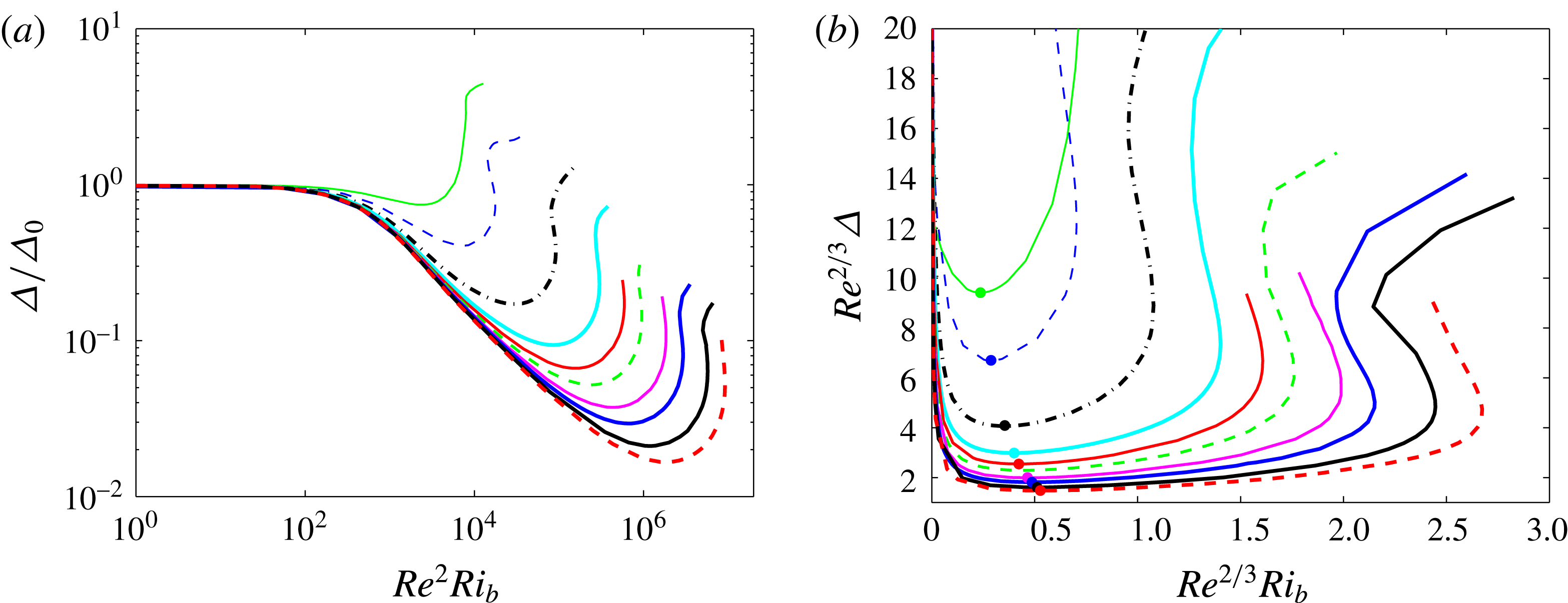
. Figure 20(a) confirms this scaling as
 $Ri_{b}$
increases from zero, which is just a statement that the Rayleigh number,
 $Ra:=-Ri_{b}Re^{2}Pr$
, is
 $O(1)$
. This scaling was proposed by Eaves & Caulfield (Reference Eaves and Caulfield2015) by heuristic arguments and has also been independently found recently by Deguchi (Reference Deguchi2017).
(a) Regime 1: wall shear stress deviation normalised by
 $\unicode[STIX]{x1D6E5}_{0}$
(its value at
 $Ri_{b}=0$
) versus
 $Re^{2}Ri_{b}$
. (b) Regime 2: compensated wall stress
 $Re^{2/3}\unicode[STIX]{x1D6E5}$
versus
 $Re^{2/3}Ri_{b}$
(colours as in figure 16). The dot on each curve marks the position of
 $Ri_{b}^{min}$
while
 $Ri_{b}^{max}$
corresponds to the rightmost turning point on each curve.

3.4.2 Regime 2
When
 $Ri_{b}\gg O(Re^{-2})$
regime 1 must give way to another regime. Figures 17 and 18 indicate that
 $\hat{\boldsymbol{u}}$
and
 $\hat{\unicode[STIX]{x1D70C}}$
localise in the spanwise and cross-stream directions yet stay global in the streamwise direction. This adjustment can be captured by the rescaling
 $$\begin{eqnarray}(\unicode[STIX]{x2202}_{y},\unicode[STIX]{x2202}_{z})\rightarrow (\unicode[STIX]{x2202}_{y},\unicode[STIX]{x2202}_{z})/\unicode[STIX]{x1D716}\quad \text{and}\quad (\bar{u},\bar{v},\bar{w},\bar{\unicode[STIX]{x1D70C}})\rightarrow (\unicode[STIX]{x1D716}\bar{u},\bar{v}/\unicode[STIX]{x1D716},\bar{w}/\unicode[STIX]{x1D716},\unicode[STIX]{x1D716}\bar{\unicode[STIX]{x1D70C}}),\end{eqnarray}$$
where
 $\unicode[STIX]{x1D716}:=(Re^{2}Ri_{b})^{-1/4}\ll 1$
for
 $Ri_{b}\gg Re^{-2}$
indicates the scale of localisation in both cross-stream and spanwise directions. This preserves the form of the equations for the roll-, streak- and streamwise-averaged density fields yet accommodates the enlarged buoyancy term in the roll equations (either (3.12) or (3.13)). The rescaling for
 $\bar{u}$
and
 $\bar{\unicode[STIX]{x1D70C}}$
comes from the fact that the streaks and
 $\bar{\unicode[STIX]{x1D70C}}$
only now extend over a cross-stream distance of
 $O(\unicode[STIX]{x1D716})$
of the underlying applied shear and density fields. A similar scaling was discussed in Blackburn, Hall & Sherwin (Reference Blackburn, Hall and Sherwin2013) for unstratified flows when considering the large spanwise wavenumber limit of the SSP/VWI process. Here, the rescaling is driven by increasing
 $Ri_{b}$
but the overall effect is the same except that there is no localisation in the streamwise direction. This rescaling accommodates increasing stratification until the spanwise localisation of the streamwise-independent fields approaches the critical layer scaling of
 $Re^{-1/3}$
, i.e. when
 $$\begin{eqnarray}\unicode[STIX]{x1D716}=O(Re^{-1/3})\rightarrow Ri_{b}=O(Re^{-2/3}).\end{eqnarray}$$
At this point, the whole perturbation velocity and density fields are confined to the critical ‘layer’, which is actually a region localised in both cross-stream and spanwise directions. In this, viscosity is important and the rolls and waves are indistinguishable, requiring a new asymptotic description. The boundary region equations (BREs) of Deguchi, Hall & Walton (Reference Deguchi, Hall and Walton2013) and Deguchi & Hall (Reference Deguchi and Hall2015) then seem the only viable rescaling to reflect this new structure. In these, a new spanwise variable
 $Z:=Re^{1/3}(z-z_{c})$
(where
 $z_{c}$
is the centre of the localised structure) is defined along with the cross-shear critical layer variable
 $Y:=Re^{1/3}y$
in regime 1. Concentrating on the vertical stratification situation and essentially following Deguchi & Hall (Reference Deguchi and Hall2015), we write
 $$\begin{eqnarray}\displaystyle & \displaystyle u=Re^{-1/3}[Y+U(x,Y,Z)]+Re^{-2/3}U_{1}(x,Y)+Re^{-1}d_{u}Y+\cdots \,, & \displaystyle\end{eqnarray}$$
 $$\begin{eqnarray}\displaystyle & \displaystyle v=Re^{-2/3}V(x,Y,Z)+Re^{-1}V_{1}(x,Y)+\cdots \,, & \displaystyle\end{eqnarray}$$
 $$\begin{eqnarray}\displaystyle & \displaystyle w=Re^{-2/3}W(x,Y,Z)+\cdots \,, & \displaystyle\end{eqnarray}$$
 $$\begin{eqnarray}\displaystyle & \displaystyle p=Re^{-4/3}\left[{\textstyle \frac{1}{2}}Ri_{b}Re^{2/3}Y^{2}+P(x,Y,Z)\right]+Re^{-5/3}P_{1}(x,Y)+\cdots \,, & \displaystyle\end{eqnarray}$$
 $$\begin{eqnarray}\displaystyle & \displaystyle \unicode[STIX]{x1D70C}=Re^{-1/3}[\!-\!Y+R(x,Y,Z)]+Re^{-2/3}R_{1}(x,Y)+Re^{-1}d_{\unicode[STIX]{x1D70C}}Y+\cdots \,. & \displaystyle\end{eqnarray}$$
The rationale behind this expansion is the realisation that the leading fields
 $(U,V,W,P,R)$
are concentrated over a reduced scale
 $O(Re^{-1/3})$
in
 $z$
so spanwise averaging produces fields that are
 $O(Re^{1/3})$
smaller; that is,
 $$\begin{eqnarray}\displaystyle & \displaystyle \langle u\rangle =y+Re^{-2/3}[U_{1}(x,Y)+d_{u}y]+\cdots \,, & \displaystyle\end{eqnarray}$$
 $$\begin{eqnarray}\displaystyle & \displaystyle \langle v\rangle =Re^{-1}V_{1}(x,Y)+\cdots \,, & \displaystyle\end{eqnarray}$$
 $$\begin{eqnarray}\displaystyle & \displaystyle \langle w\rangle =0\text{ (by symmetry)}, & \displaystyle\end{eqnarray}$$
 $$\begin{eqnarray}\displaystyle & \displaystyle \langle p\rangle ={\textstyle \frac{1}{2}}Ri_{b}y^{2}+Re^{-5/3}P_{1}(x,Y)+\cdots \,, & \displaystyle\end{eqnarray}$$
 $$\begin{eqnarray}\displaystyle & \displaystyle \langle \unicode[STIX]{x1D70C}\rangle =-y+Re^{-2/3}[R_{1}(x,Y)+d_{\unicode[STIX]{x1D70C}}y]+\cdots \,, & \displaystyle\end{eqnarray}$$
since
 $y=Re^{-1/3}Y$
and
 $$\begin{eqnarray}\langle (U,V,W,P,R)\rangle =(0,0,0,0,0)\quad \text{where }\langle (\quad )\rangle :={\displaystyle \frac{1}{L_{z}}}\int _{0}^{L_{z}}(\quad )\,\text{d}z.\end{eqnarray}$$
These scalings give the leading balance
 $$\begin{eqnarray}\displaystyle & \displaystyle (Y+U)U_{x}+V(1+U_{Y})+WU_{Z}=U_{YY}+U_{ZZ}, & \displaystyle\end{eqnarray}$$
 $$\begin{eqnarray}\displaystyle & \displaystyle (Y+U)V_{x}+VV_{Y}+WV_{Z}+P_{Y}=V_{YY}+V_{ZZ}-Ri_{b}Re^{2/3}R, & \displaystyle\end{eqnarray}$$
 $$\begin{eqnarray}\displaystyle & \displaystyle (Y+U)W_{x}+VW_{Y}+WW_{Z}+P_{Z}=W_{YY}+W_{ZZ}, & \displaystyle\end{eqnarray}$$
 $$\begin{eqnarray}\displaystyle & \displaystyle U_{x}+V_{Y}+W_{Z}=0, & \displaystyle\end{eqnarray}$$
 $$\begin{eqnarray}\displaystyle & \displaystyle UR_{x}+V(-1+R_{Y})+WR_{Z}={\displaystyle \frac{1}{Pr}}(R_{YY}+R_{ZZ}), & \displaystyle\end{eqnarray}$$
to be solved with periodic boundary conditions in
 $x$
and asymptotically decaying boundary conditions
 $(U,V,W,R)\rightarrow (0,0,0,0)$
as
 $Y,Z\rightarrow \pm \infty$
since no other possibility with vanishing spanwise average can connect to linear profiles in an unforced exterior. The spanwise-averaged problem is
 $$\begin{eqnarray}\displaystyle & \displaystyle \langle (U^{2})_{x}+(UV)_{Y}\rangle =U_{1,YY}, & \displaystyle\end{eqnarray}$$
 $$\begin{eqnarray}\displaystyle & \displaystyle \langle (UV)_{x}+(V^{2})_{Y}\rangle =V_{1,YY}-P_{1,Y}-Ri_{b}Re^{2/3}R_{1}, & \displaystyle\end{eqnarray}$$
 $$\begin{eqnarray}\displaystyle & \displaystyle 0=U_{1,x}+V_{1,Y}, & \displaystyle\end{eqnarray}$$
 $$\begin{eqnarray}\displaystyle & \displaystyle \langle (UR)_{x}+(VR)_{Y}\rangle ={\displaystyle \frac{1}{Pr}}R_{1,YY}. & \displaystyle\end{eqnarray}$$
The problem (3.54)–(3.57) is then really just one in
 $U_{1}$
and
 $R_{1}$
, which are each computed by two quadratures of (3.54) and (3.57) respectively (
 $V_{1}$
is then found by one quadrature of
 $-U_{1,x}$
and
 $P_{1}$
follows from (3.55)). In fact, all the computed solutions indicate that
 $U=-R$
(recall
 $Pr=1$
) – for example see figure 19 – and hence
 $U_{1}=-R_{1}$
. The spanwise-averaged problem then boils down to solving (3.54), which requires
 $\langle (U^{2})_{x}\rangle$
integrated twice and
 $\langle (UV)\rangle$
integrated once with respect to
 $Y$
. Assuming that
 $U$
and
 $V$
vanish fast enough as
 $Y\rightarrow \pm \infty$
, the first term can be expected to drive a particular solution for
 $U_{1}$
odd in
 $Y$
(as
 $\langle (U^{2})_{x}\rangle$
is odd in
 $Y$
) with limiting behaviour
 $A(x)Y$
for some function
 $A(x)$
. This behaviour must be eliminated by the complementary solution, or else a mean flow correction of
 $O(Re^{1/3})$
arises in the exterior which is inconsistent with (3.48). Integrating
 $\langle (UV)\rangle$
once can be expected to drive a particular solution for
 $U_{1}$
which asymptotes to one function
 $B(x)-d_{u}(x)$
for
 $Y\rightarrow \infty$
and another function
 $B(x)+d_{u}(x)$
for
 $Y\rightarrow -\infty$
as
 $\langle (\mathit{UV})\rangle$
has no particular symmetry in
 $Y$
. Given the need to match onto simple shears and density gradients in the exterior dependent only on
 $y$
and the antisymmetry of the mean flow and density gradient,
 $B$
and
 $d_{u}$
must be simple constants and a further contribution from the complementary solution of the form
 $-B$
needs to be invoked to antisymmetrise the limiting asymptotic behaviour. Hence, a solution for
 $U_{1}$
should be sought with
 $(U_{1},V_{1},W_{1},R_{1})\rightarrow (\mp d_{u},0,0,\pm d_{\unicode[STIX]{x1D70C}})$
as
 $Y\rightarrow \pm \infty$
(with
 $d_{\unicode[STIX]{x1D70C}}=-d_{u}$
inferred by observation). These boundary conditions together with the expansions in (3.38) and (3.42) ensure that the exterior solution just represents a shifted shear in
 $u$
and gradient in
 $\unicode[STIX]{x1D70C}$
consistent with the imposed conditions on
 $y=\pm 1$
(see Deguchi & Hall Reference Deguchi and Hall2014, Reference Deguchi and Hall2015). The upshot of all this is a prediction for the mean shear deviation
 $\unicode[STIX]{x1D6E5}$
of
 $d_{u}Re^{-2/3}$
as in Deguchi & Hall (Reference Deguchi and Hall2015) in this second regime – regime 2 – which is reached when
 $Ri_{b}=O(Re^{-2/3})$
(see (3.50) and (3.55)). In the unstratified situation, the BRE regime is only reached when the streamwise wavenumber
 $\unicode[STIX]{x1D6FC}$
becomes
 $O(Re^{-1})$
, at which point the critical layer expands to fill the domain (Deguchi, Hall & Walton Reference Deguchi, Hall and Walton2013). Stable stratification, however, causes this regime to be realised for
 $\unicode[STIX]{x1D6FC}=O(1)$
when
 $Ri_{b}\sim Re^{-2/3}$
. The effect of both spanwise and cross-stream localisation of the flow is to reduce the regions where the flow is directed against gravity and hence to keep the potential energy low. In fact,
 $E_{p}$
stays
 $O(Re^{-2})$
as in regime 1 and remains comparable to
 $E_{k}^{v}$
when
 $Ri_{b}=O(Re^{-2/3})$
.
Selected profiles through the streamwise velocity perturbation at
 $Ri_{b}^{max}$
for
 $Re/10\,000=1$
,
 $2$
,
 $4$
,
 $6$
and
 $8$
. (a)
 $Re^{1/3}u(x,y_{c}(Re/10\text{,}000),z_{c})$
versus
 $x$
where
 $y_{c}(1)=0.0675$
,
 $y_{c}(2)=0.0575$
,
 $y_{c}(4)=0.05$
,
 $y_{c}(6)=0.04$
and
 $y_{c}(8)=0.035$
are the approximate levels of the streak core shown, for example, in figure 17(d) for
 $Re=40\,000$
. (b)
 $Re^{1/3}u(0,y,z_{c})$
versus
 $Re^{1/3}y$
where
 $z_{c}\approx 0.83$
is the spanwise position of the (a,c) streak core. (c)
 $Re^{1/3}u(0,y_{c}(Re),z)$
versus
 $Re^{1/3}(z-z_{c})$
(colours as in figure 16). (d)
 $Ri_{b}^{min}(Re)$
(blue line with dots) where
 $\unicode[STIX]{x1D6E5}$
reaches a minimum as
 $Ri_{b}$
increases from zero and
 $Ri_{b}^{max}(Re)$
(red line with open squares) where the
 $\unicode[STIX]{x1D6E5}-Ri_{b}$
curve turns around versus
 $Re$
. The dashed black guideline indicates a scaling of
 $Re^{-2/3}$
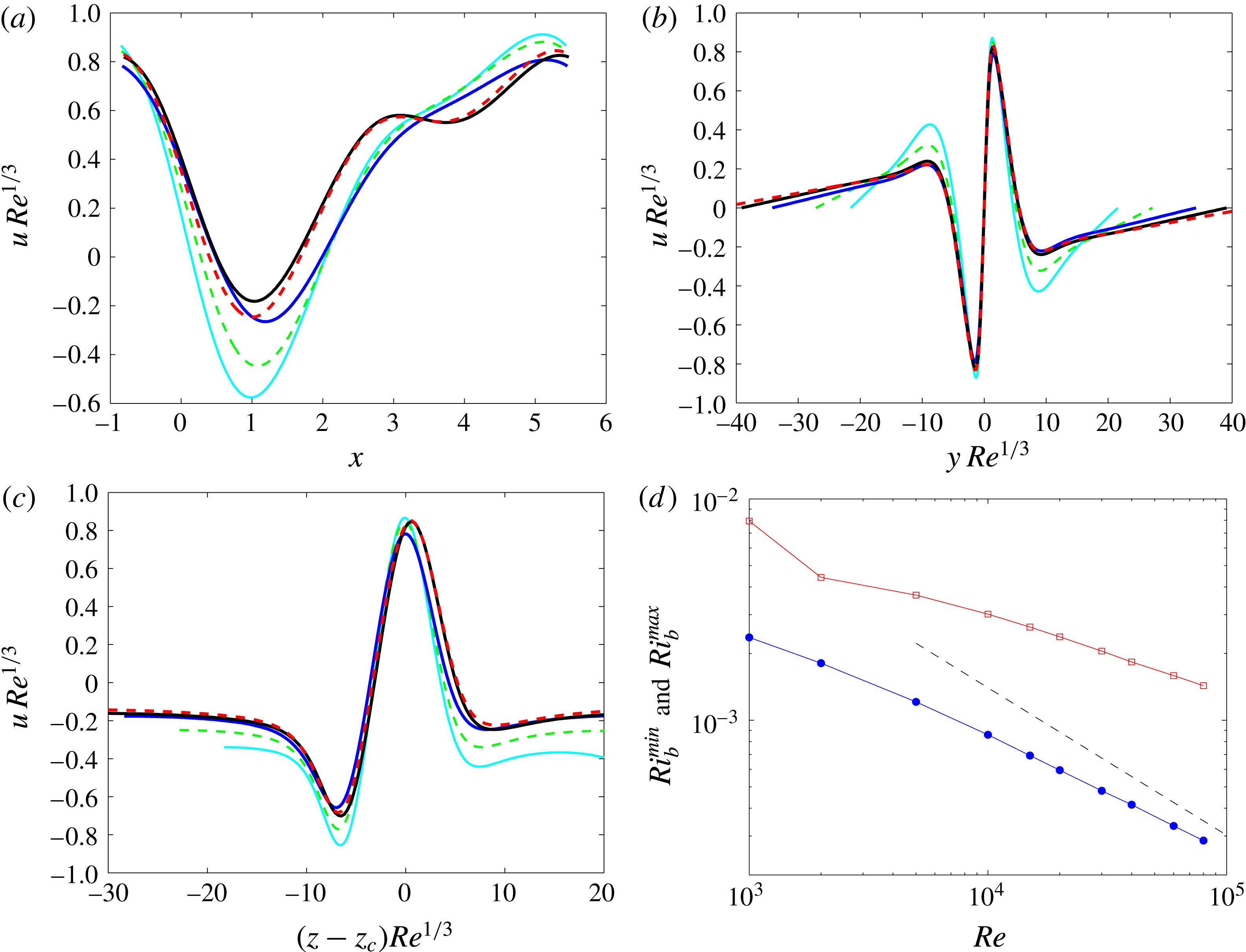
.

The plot in figure 20(b) shows that plotting
 $Re^{2/3}\unicode[STIX]{x1D6E5}$
versus
 $Re^{2/3}Ri_{b}$
does a good job of collapsing the data for
 $Re\in [10\,000,80\,000]$
as far as
 $Ri_{b}^{min}$
is concerned, i.e. the region around the stress deviation minimum. The collapse, however, is not compelling near
 $Ri_{b}^{max}$
and suggests the presence of a third regime valid for
 $Ri_{b}\gg Re^{-2/3}$
. Figure 18 gives some tentative evidence for this – see the transition from
 $Ri_{b}^{min}(40\,000)$
(bottom left plot) to
 $Ri_{b}^{max}(40\,000)$
(bottom right) – and
 $Ri_{b}^{max}$
does not appear to be scaling with
 $Re^{-2/3}$
, unlike
 $Ri_{b}^{min}$
(see figure 21
d). When
 $Ri_{b}\gg Re^{-2/3}$
, a further rescaling of the vertical momentum equation (3.50) is required to balance the increased buoyancy term. Specifically,
 $$\begin{eqnarray}(\unicode[STIX]{x2202}_{x},\unicode[STIX]{x2202}_{Y},\unicode[STIX]{x2202}_{Z})\rightarrow (\unicode[STIX]{x2202}_{x}/\unicode[STIX]{x1D6FF}^{\ast },\unicode[STIX]{x2202}_{Y}/\unicode[STIX]{x1D700},\unicode[STIX]{x2202}_{Z}/\unicode[STIX]{x1D700})\quad \text{and}\quad (U,V,W,R)\rightarrow (\unicode[STIX]{x1D700}U,V/\unicode[STIX]{x1D700},W/\unicode[STIX]{x1D700},\unicode[STIX]{x1D700}R),\end{eqnarray}$$
where balancing advective, diffusive and buoyancy terms requires
 $$\begin{eqnarray}\unicode[STIX]{x1D700}=Ri_{b}^{-1/4}Re^{-1/6}\quad \text{and}\quad \unicode[STIX]{x1D6FF}^{\ast }=Ri_{b}^{-3/4}Re^{-1/2}.\end{eqnarray}$$
This represents a total rescaling of
 $$\begin{eqnarray}\displaystyle & \displaystyle (\unicode[STIX]{x2202}_{x},\unicode[STIX]{x2202}_{y},\unicode[STIX]{x2202}_{z})\rightarrow (Ri_{b}^{3/4}Re^{1/2}\unicode[STIX]{x2202}_{x},Ri_{b}^{1/4}Re^{1/2}[\unicode[STIX]{x2202}_{y},\unicode[STIX]{x2202}_{z}]), & \displaystyle\end{eqnarray}$$
 $$\begin{eqnarray}\displaystyle & \displaystyle (u,v,w,\unicode[STIX]{x1D70C})\rightarrow Ri_{b}^{-1/4}Re^{1/2}(u,v,w,\unicode[STIX]{x1D70C}). & \displaystyle\end{eqnarray}$$
When
 $Ri_{b}=O(1)$
, the length scales in
 $x,y$
and
 $z$
become comparable and streamwise diffusion must be reintroduced. At this point, all terms in the momentum equation are important and the local Reynolds number is 1 (Deguchi (Reference Deguchi2015) calls this the ‘unit Reynolds number Navier–Stokes equations’ or UNS regime). Explicitly, rescaling the total fields as
 $$\begin{eqnarray}(\unicode[STIX]{x2202}_{x},\unicode[STIX]{x2202}_{y},\unicode[STIX]{x2202}_{z})\rightarrow Re^{1/2}(\unicode[STIX]{x2202}_{x},\unicode[STIX]{x2202}_{y},\unicode[STIX]{x2202}_{z})\quad \text{and}\quad (u,v,w,\unicode[STIX]{x1D70C},p)\rightarrow (Re^{-1/2}[u,v,w,\unicode[STIX]{x1D70C}],Re^{-1}p)\end{eqnarray}$$
converts the Boussinesq equations (3.1)–(3.5) to
 $$\begin{eqnarray}\displaystyle & \displaystyle u_{t}+uu_{x}+vu_{y}+wu_{z}+p_{x}=\unicode[STIX]{x1D6FB}^{2}u, & \displaystyle\end{eqnarray}$$
 $$\begin{eqnarray}\displaystyle & \displaystyle v_{t}+uv_{x}+vv_{y}+wv_{z}+p_{y}=\unicode[STIX]{x1D6FB}^{2}v-Ri_{b}\;\unicode[STIX]{x1D70C}\cos \unicode[STIX]{x1D703}, & \displaystyle\end{eqnarray}$$
 $$\begin{eqnarray}\displaystyle & \displaystyle w_{t}+uw_{x}+vw_{y}+ww_{z}+p_{z}=\unicode[STIX]{x1D6FB}^{2}w-Ri_{b}\;\unicode[STIX]{x1D70C}\sin \unicode[STIX]{x1D703}, & \displaystyle\end{eqnarray}$$
 $$\begin{eqnarray}\displaystyle & \displaystyle \unicode[STIX]{x1D70C}_{t}+u\unicode[STIX]{x1D70C}_{x}+v\unicode[STIX]{x1D70C}_{y}+w\unicode[STIX]{x1D70C}_{z}={\displaystyle \frac{1}{Pr}}\unicode[STIX]{x1D6FB}^{2}\unicode[STIX]{x1D70C}, & \displaystyle\end{eqnarray}$$
 $$\begin{eqnarray}\displaystyle & \displaystyle u_{x}+v_{y}+w_{z}=0, & \displaystyle\end{eqnarray}$$
where now asymptotic boundary conditions
 $(u,v,w,\unicode[STIX]{x1D70C})\rightarrow (\pm y,0,0,\mp y)$
as
 $y\rightarrow \pm \infty$
should be imposed. In this regime, the viscous diffusion time, the advective (turnover) time and the buoyancy time scale are all the same since the local Richardson number (which is the same as
 $Ri_{b}$
here) is
 $O(1)$
. Assuming the dissipation rate has a laminar scaling,
 $\unicode[STIX]{x1D6F7}=O(1/Re)$
, this corresponds to the statement that the
 $O(Re^{-1/2})$
length scale of the flow corresponds to both the Kolmogorov length scale
 $(\unicode[STIX]{x1D6F7}Re^{3})^{-1/4}$
and the Osmidov length scale
 $(\unicode[STIX]{x1D6F7}Ri_{b}^{-3/2})^{1/2}$
and therefore is minimal, i.e. the equations cannot support a smaller scale (Deguchi Reference Deguchi2017). This third regime then seems the ultimate regime as increasing
 $Ri_{b}$
above
 $O(1)$
would lead to a stabilising buoyancy force which could not be overcome by rescaling further: the solutions would simply cease to exist.
Since this third regime has localisation in all three directions, reaching it presents a considerable numerical challenge. Of the numerical solutions obtained, the streamwise gradients appear to stay
 $O(1)$
even at
 $Re=80\,000$
compared to the spanwise and cross-stream gradients: see figure 21 which plots
 $\hat{u} Re^{1/3}$
over the three directions for
 $Re=10\,000,20\,000,40\,000$
and
 $80\,000$
at
 $Ri_{b}^{max}(Re)$
. The localisation length scale of
 $O(Re^{-1/3})$
is well established in the
 $y$
(cross-stream) and
 $z$
(spanwise) directions, whereas the profiles in the
 $x$
(streamwise) direction show no tendency to steepen with increasing
 $Re$
. One strategy adopted by Deguchi (Reference Deguchi2017) to reach this regime is to force the flow to develop steep streamwise gradients by shrinking the computational box. The flow necessarily stays strictly periodic in both spanwise and streamwise directions as opposed to showing localisation, but some evidence of this third regime can nevertheless then be found: see figure 4 of Deguchi (Reference Deguchi2017).
4 Discussion
We first summarise the findings of the paper, in which we have considered stratified plane Couette flow where a stable density gradient is applied via Dirichlet boundary conditions on the flow.
(1) Laminar–turbulent boundary. Stratification increases the number of non-dimensional parameters specifying the system from 1 (
 $Re$
) to 3 (
 $Re,\,Ri_{b},\,Pr$
). Reducing this number to 2 by setting
 $Pr=1$
throughout, an approximate characterisation
 $Ri_{b}^{c}(Re)$
of the laminar–turbulent boundary in parameter space – the
 $(Re,Ri_{b})$
plane – has been made which shows that
 $Ri_{b}^{c}$
is a monotonically increasing function of
 $Re$
for
 $Re\leqslant 5000$
. Of the two geometries considered, the larger computational box allows turbulence to reach slightly higher values of
 $Ri_{b}^{c}$
at a given
 $Re$
. Approaching this boundary by decreasing
 $Re$
at small fixed
 $Ri_{b}$
leads to the same situation as in unstratified flow where the turbulent attractor eventually collides with the laminar–turbulent boundary in phase space. In contrast, when the laminar–turbulent boundary is approached in parameter space by fixing
 $Re$
and increasing
 $Ri_{b}$
, the turbulent attractor expands, displaying larger and larger fluctuations until ultimately it touches the laminar–turbulent boundary in phase space.
(2) Edge tracking and ECS. In order to understand this laminar–turbulent boundary, ECS were sought which exist beyond this (at higher
 $Ri_{b}$
) in the
 $(Re,Ri_{b})$
plane. Edge tracking was performed for two reasons: (i) to select relevant ECS (otherwise unstratified states would have to be selected arbitrarily to continue to
 $Ri_{b}\neq 0$
); and (ii) to possibly find new states of non-SSP/VWI type. Despite investigating a number of different geometries, various parameter settings of
 $Re$
and
 $Ri_{b}$
, and combinations of imposed symmetries, only two simple states were found as edge states (the rest being chaotic). These states when continued back to
 $Ri_{b}=0$
turned out to be EQ7 and EQ7-1 of Gibson & Brand (Reference Gibson and Brand2014). No new states of non-SSP/VWI were found.
(3) Connections with 2-D convective roll solutions. Continuing EQ7-1, which is spanwise localised at
 $Ri_{b}=0$
, to unstable stratifications (
 $Ri_{b}<0$
) revealed an interestingly simple delocalisation process whereupon the exponentially decaying tails gradually reduce their spatial decay rate to zero at a bifurcation point off a (spanwise global) 2-D convective roll branch of solutions. EQ7 was similarly tracked back to a bifurcation off a (double layer) branch of 2-D convective rolls as was Nagata’s (Reference Nagata1990) solution (confirming Clever & Busse Reference Clever and Busse1992, Reference Clever, Busse, Egbers and Pfister2000).
(4) Strong influence of stable stratification. Continuing these solutions to
 $Ri_{b}>0$
showed that stable stratification has a surprisingly strong effect on the SSP/VWI mechanisms. A simple connection between upper and lower EQ7 branches traced by allowing
 $Ri_{b}$
to change continuously for
 $Re\leqslant 400$
is broken by
 $Re=500$
, revealing another branch of states which apparently give rise to new unstratified solutions (see figure 15). The lower branch of EQ7 solutions undergoes a further topological change by
 $Re=850$
so that the solutions for
 $Ri_{b}>0$
become increasingly convoluted. Nagata’s solution is also found to bifurcate off EQ7 for non-zero stable stratification.
(5) Asymptotics. Calculations for low
 $Re$
(
 ${\leqslant}1000$
) indicate that EQ7 of the three types of solutions considered could survive to the highest levels of stratification. High-
 $Re$
(up to
 $80\,000$
) calculations were then done for EQ7, which revealed two regimes and hinted at a third. The first regime is characterised by
 $Ri_{b}=O(Re^{-2})$
– or Rayleigh number
 $Ra:=-Ri_{b}Re^{2}Pr=O(1)$
– where the SSP/VWI process underpinning EQ7 starts to feel the stratification. For
 $Ri_{b}\gg Re^{-2}$
, EQ7 progressively localises in both the spanwise and cross-stream directions until at
 $Ri_{b}=O(Re^{-2/3})$
the localisation is on the scale of the critical layer. This signals the second regime where the asymptotic structure is described by a stratified version of the BREs of Deguchi, Hall & Walton (Reference Deguchi, Hall and Walton2013) and Deguchi & Hall (Reference Deguchi and Hall2015). For even larger
 $Ri_{b}$
, the stabilising buoyancy force can be counterbalanced by further localisation which now has to include streamwise localisation until an ultimate third regime where
 $Ri_{b}=O(1)$
appears possible. Here the scale of the flow in all three directions is simultaneously the minimal Kolmogorov scale and the Osmidov length scale, i.e. viscous, advective and buoyancy time scales all match. Numerical solutions indicate a transition out of the second regime but could not capture the third regime due to resolution issues.
One of the main findings of this work is that stable stratification has such a strong effect on the finite-amplitude states considered here. Bulk Richardson numbers of
 $O(Re^{-2})$
(actually an
 $O(1)$
Rayleigh number for
 $Pr=O(1)$
) are already enough to start modifying the SSP/VWI process which underpins all known ECS in PCF. To put this into some context, consider flow along a pipe of diameter
 $D$
across which a temperature difference of
 $\unicode[STIX]{x1D6FF}T$
is unwittingly applied. One can expect this temperature difference to have a significant effect on, say, measured wall stresses or phase speeds of ECS if
 $Ri_{b}Re^{2}=-Ra/Pr=10^{3}$
(see appendix B and figure 20) where
 $Ra:=\unicode[STIX]{x1D6FC}g\unicode[STIX]{x1D6FF}TD^{3}/\unicode[STIX]{x1D708}^{2}$
. Using the volumetric coefficient of thermal expansion for water at
 $20\,^{\circ }\text{C}$
,
 $\unicode[STIX]{x1D6FC}=2\times 10^{-4}~\text{K}^{-1}$
,
 $g=9.8~\text{m}~\text{s}^{-2}$
,
 $D=0.02~\text{m}$
and
 $\unicode[STIX]{x1D708}=10^{-6}~\text{m}^{2}~\text{s}^{-1}$
gives
 $\unicode[STIX]{x1D6FF}T=6.4\times 10^{-2}~\text{K}$
, which is not particularly large (of course this would have to be applied consistently along the pipe and the fluid present in the pipe long enough to feel the imposed temperature difference).
Increasing the stratification further causes the ECS to progressively localise to reduce the potential energy penalty for vertical motions imposed by stable stratification. This occurs firstly in the spanwise and cross-stream directions and then in all three directions when
 $Ri_{b}\gg Re^{-2/3}$
. Ultimately, the scale of localisation becomes the minimal possible in all three directions at
 $Ri_{b}=O(1)$
for large
 $Re$
. The idealised plane Couette flow set-up analysed here of course imposes a specific shear and a density gradient through the boundary conditions. In more general flow conditions, the local shear and density gradient as measured by a gradient Richardson number
 $Ri$
will vary so that a hierarchy of ECS with different length scales can exist in the same flow. The general conclusion of this work is that the smaller the length scale of the ECS the larger the local
 $Ri$
which can be accommodated. For example, large-scale flows can only accommodate
 $Ri=O(Re^{-2})$
levels of stratification, whereas ECS on the scale of the Kolmogorov length can survive even when
 $Ri=O(1)$
. The existence of these latter localised states means that there is no reason to doubt that stratified turbulence could not be present at
 $Ri_{b}=O(1)$
as
 $Re\rightarrow \infty$
. Confirming this scenario is an important future challenge.
A question which has been left unanswered by this study is the possible existence of new types of finite-amplitude states which have no counterpart in the unstratified situation. Probing this issue would appear to require
 $O(1)$
Richardson numbers (so the time scale of internal gravity waves match the advective time scale), which it is now clear requires large
 $Re$
certainly beyond what has been studied numerically here. This and the issue of how the Prandtl number affects the solutions found here are important questions for future study.
Finally, it is interesting but perhaps not surprising that all of the three ECS studied here can be traced back to bifurcations off (primary) 2-D convective roll solutions in sheared Rayleigh–Bénard convection. Given that 2-D finite-amplitude rolls in sheared Rayleigh–Bénard convection are essentially the same as in unsheared Rayleigh–Bénard convection (e.g. the shear only acts to remove the degeneracy in the bifurcating roll orientation having no effect on the bifurcation point itself – Kelly (Reference Kelly and Spaulding1977)), it is hard not to speculate that all ECS in unstratified PCF are actually born in bifurcations which can be traced back to the linear instability problem in Rayleigh–Bénard convection.
Acknowledgements
After this work was submitted, we became aware of a closely related study by Deguchi (Reference Deguchi2017). The authors thank him for sharing his preprint. D.O. would like to thank CONACYT for the award of a scholarship which has supported his PhD studies and the availability of free HPC time on the University of Bristol’s BlueCrystal supercomputer. Both D.O. and R.R.K. thank the MUST team at Cambridge (C. Caulfield, S. Dalziel, P. Linden and J. Taylor amongst others) for stimulating conversations and their interest in this work. R.R.K. would also like to thank P. Linden for asking about temperature effects in pipe flow.
Appendix A
A direct Newton–Raphson solver was used to track EQ7 around in parameter space. The velocity representation for a highly symmetric (i.e. possesses
 ${\mathcal{S}}$
,
 $\unicode[STIX]{x1D6FA}$
and
 ${\mathcal{Z}}$
symmetries) steady structure is
 $$\begin{eqnarray}\left[\begin{array}{@{}c@{}}u\\ v\\ w\\ p\\ \unicode[STIX]{x1D70C}\end{array}\right]=\left[\begin{array}{@{}r@{}}y\\ 0\\ 0\\ 0\\ -y\end{array}\right]+\mathop{\sum }_{n=1}^{N}\mathop{\sum }_{\begin{array}{@{}c@{}}m,\ell =0,\\ m+\ell \,\text{even}\end{array}}^{M,L}\left[\begin{array}{@{}c@{}}(u_{nm\ell }^{(r)}\unicode[STIX]{x1D6F7}_{o}(y)+iu_{nml}^{(i)}\unicode[STIX]{x1D6F7}_{e}(y))\cos \ell \unicode[STIX]{x1D6FD}z\\ (v_{nm\ell }^{(r)}\unicode[STIX]{x1D6F7}_{o}(y)+iv_{nml}^{(i)}\unicode[STIX]{x1D6F7}_{e}(y))\cos \ell \unicode[STIX]{x1D6FD}z\\ (w_{nm\ell }^{(r)}\unicode[STIX]{x1D6F7}_{o}(y)+iw_{nml}^{(i)}\unicode[STIX]{x1D6F7}_{e}(y))\sin \ell \unicode[STIX]{x1D6FD}z\\ (p_{nm\ell }^{(r)}\unicode[STIX]{x1D6F9}_{e}(y)+ip_{nml}^{(i)}\unicode[STIX]{x1D6F9}_{o}(y))\cos \ell \unicode[STIX]{x1D6FD}z\\ (\unicode[STIX]{x1D70C}_{nm\ell }^{(r)}\unicode[STIX]{x1D6F7}_{o}(y)+i\unicode[STIX]{x1D70C}_{nml}^{(i)}\unicode[STIX]{x1D6F7}_{e}(y))\cos \ell \unicode[STIX]{x1D6FD}z\\ \end{array}\right]\text{e}^{\text{i}m\unicode[STIX]{x1D6FC}x}+\text{c.c.}\end{eqnarray}$$
The cross-stream basis functions
 $\unicode[STIX]{x1D6F7}_{e},\unicode[STIX]{x1D6F9}_{e}$
(even in
 $y$
) and
 $\unicode[STIX]{x1D6F7}_{o},\unicode[STIX]{x1D6F9}_{o}$
(odd in
 $y$
) were defined in two ways depending on whether one (Code 1) or two (Code 2) spectral elements were used. In Code 1,
 $$\begin{eqnarray}\displaystyle & \displaystyle [\unicode[STIX]{x1D6F7}_{o}(y),\unicode[STIX]{x1D6F7}_{e}(y)]:=[T_{2n+1}(y)-T_{2n-1}(y),~T_{2n}(y)-T_{2n-2}(y)\,], & \displaystyle\end{eqnarray}$$
 $$\begin{eqnarray}\displaystyle & \displaystyle [\unicode[STIX]{x1D6F9}_{o}(y),\unicode[STIX]{x1D6F9}_{e}(y)]:=[T_{2n-1}(y),~T_{2n-2}(y)], & \displaystyle\end{eqnarray}$$
with Dirichlet boundary conditions built into the bases
 $\unicode[STIX]{x1D6F7}_{e}$
and
 $\unicode[STIX]{x1D6F7}_{o}$
. The equations then only needed to be collocated over half the domain, so the points
 $$\begin{eqnarray}-1\,<\,y_{j}:=\cos \biggl[{\displaystyle \frac{\unicode[STIX]{x03C0}(2(j+N)-1)}{4N}}\biggr]<0,\quad j=1,\ldots ,N\end{eqnarray}$$
were used. In Code 2, the half-interval
 $[-1,0]$
was split into two domains
 $[-1,y_{p}]$
and
 $[y_{p},0]$
where
 $y_{p}$
typically was chosen as
 $-0.1$
or
 $-0.2$
. Then the following definitions were made:
 $$\begin{eqnarray}\displaystyle [\unicode[STIX]{x1D6F7}_{o}(y),\unicode[STIX]{x1D6F7}_{e}(y)]:=\left\{\begin{array}{@{}ll@{}}[\,T_{2n-1}(-y/y_{p}),\,\,T_{2n-2}(-y/y_{p})], & y_{p}\,<\,y\,<\,0,\\ \text{}[\,T_{n}(\overline{y})+T_{n-1}(\overline{y}),\,\,T_{n}(\overline{y})+T_{n-1}(\overline{y})], & -1\,<\,y\,<\,y_{p},\end{array}\right. & & \displaystyle\end{eqnarray}$$
 $$\begin{eqnarray}\displaystyle [\unicode[STIX]{x1D6F9}_{o}(y),\unicode[STIX]{x1D6F9}_{e}(y)]:=\left\{\begin{array}{@{}ll@{}}[\,T_{2n-1}(-y/y_{p}),\,\,T_{2n-2}(-y/y_{p})], & y_{p}\,<\,y\,<\,0,\\ \text{}[\,T_{n-1}(\overline{y}),\,\,T_{n-1}(\overline{y})], & -1\,<\,y\,<\,y_{p},\end{array}\right. & & \displaystyle\end{eqnarray}$$
where
 $\overline{y}:=(2y-y_{p}+1)/(1+y_{p})$
(again
 $\unicode[STIX]{x1D6F7}_{o}$
and
 $\unicode[STIX]{x1D6F7}_{e}$
incorporate the Dirichlet boundary conditions), and collocation was performed over the points
 $$\begin{eqnarray}y_{j}:=\left\{\begin{array}{@{}ll@{}}-y_{p}\cos \left[{\displaystyle \frac{\unicode[STIX]{x03C0}(2(j+N_{p})-1)}{4N_{p}}}\right], & j=1,\ldots ,N_{p},\\ {\displaystyle \frac{1}{2}}(y_{p}+1)\cos \left[{\displaystyle \frac{\unicode[STIX]{x03C0}(2(j-N_{p})-1)}{2(N-N_{p})}}\right]+{\displaystyle \frac{1}{2}}(y_{p}-1), & j=N_{p}+1,\ldots ,N.\end{array}\right.\end{eqnarray}$$
Continuity of the zeroth and first derivatives of all the variables
 $[u,v,w,p,\unicode[STIX]{x1D70C}]$
was then imposed at
 $y=y_{p}$
to match the spectral representations in the two domains (replacing the
 $j=N_{p}$
and
 $N_{p}+1$
collocated equation constraints). The choice
 $N-N_{p}=2N_{p}$
balances the spectral orders in the two domains and seemed to offer the best compromise between resolving the mid-plane area and allowing effective matching at
 $y=y_{p}$
.
In Code 1, the resolution near the mid-plane is
 ${\approx}1/2N$
, whereas in Code 2 it is
 ${\approx}|y_{p}|/2N_{p}$
, which is
 ${\approx}3|y_{p}|/2N$
if the choice
 $N-N_{p}=2N_{p}$
is made. Choosing
 $y_{p}=-0.1$
therefore increases the mid-plane resolution by a factor of over 3 for the same choice of
 $N$
. Multithreaded OPENBLAS libraries allowed large resolutions to be handled. Typically, up to 125 000 degrees of freedom (requiring
 ${\leqslant}$
128 GB of storage) were used – e.g.
 $(M,N,L)=(6,100,30)$
or
 $(10,50,20)$
– with some runs performed using close to 175 000 degrees of freedom (and up to 256 GB storage) – e.g.
 $(M,N,L)=(6,140,35)$
or
 $(18,75,24)$
.
Appendix B
In the normal Rayleigh–Bénard set-up (e.g. Drazin & Reid (Reference Drazin and Reid1981) equations (8.6)–(8.8) with nonlinearities reinstated) the fully nonlinear equations for the total flow field
 $\boldsymbol{U}$
and temperature field
 $\unicode[STIX]{x1D6E9}$
are
 $$\begin{eqnarray}\displaystyle & \displaystyle {\displaystyle \frac{\unicode[STIX]{x2202}\,\boldsymbol{U}}{\unicode[STIX]{x2202}\unicode[STIX]{x1D70F}}}+\boldsymbol{U}\boldsymbol{\cdot }\unicode[STIX]{x1D735}\boldsymbol{U}=-\unicode[STIX]{x1D735}P+Ra\,Pr\,\unicode[STIX]{x1D6E9}\,{\hat{y}}+Pr\unicode[STIX]{x1D6FB}^{2}\boldsymbol{U}, & \displaystyle\end{eqnarray}$$
 $$\begin{eqnarray}\displaystyle & \displaystyle {\displaystyle \frac{\unicode[STIX]{x2202}\,\unicode[STIX]{x1D6E9}}{\unicode[STIX]{x2202}\,\unicode[STIX]{x1D70F}}}+\boldsymbol{U}\boldsymbol{\cdot }\unicode[STIX]{x1D735}\unicode[STIX]{x1D6E9}=\unicode[STIX]{x1D6FB}^{2}\unicode[STIX]{x1D6E9}, & \displaystyle\end{eqnarray}$$
 $$\begin{eqnarray}\displaystyle & \displaystyle \unicode[STIX]{x1D735}\boldsymbol{\cdot }\boldsymbol{U}=0, & \displaystyle\end{eqnarray}$$
subject to boundary conditions
 $$\begin{eqnarray}u(x,\pm 1,z,t)=\pm 1\quad \text{and}\quad \unicode[STIX]{x1D703}(x,\pm 1,z,t)=\mp 1.\end{eqnarray}$$
Stratified plane Couette flow (as described by equations (2.1)–(2.3)) is retrieved under the transformation
 $$\begin{eqnarray}t=(Re\,Pr)\unicode[STIX]{x1D70F},\quad \boldsymbol{u}=\boldsymbol{U}/(Re\,Pr),\quad \unicode[STIX]{x1D70C}=\unicode[STIX]{x1D6E9},\quad p=P/(Re\,Pr)^{2}\end{eqnarray}$$
so that
 $Ra=-Ri_{b}\,Re^{2}\,Pr$
. The critical
 $Ra$
for linear instability is
 $Ra_{crit}:=1708/16$
, which is unchanged by introducing a unidirectional shear (e.g. Kelly Reference Kelly and Spaulding1977). (The factor of
 $1/16$
arises because the half-channel width has been used to non-dimensionalise the system.)
The critical
 $Re$
for energy stability,
 $Re_{ES}$
, for this system is as follows (Joseph Reference Joseph1966):
 $$\begin{eqnarray}Re_{ES}=\left\{\begin{array}{@{}ll@{}}\textstyle \frac{1}{2}\sqrt{1708}, & Ri_{b}>0,\\ \textstyle \frac{1}{2}\sqrt{1708}/\sqrt{1+4Pr(-Ri_{b})}, & Ri_{b}<0.\end{array}\right.\end{eqnarray}$$
Alternatively, the Rayleigh–Bénard problem with shear has an energy stability threshold,
 $Ra_{ES}$
, given by
 $$\begin{eqnarray}Ra_{ES}=Ra_{crit}-\textstyle \frac{1}{4}Re^{2},\end{eqnarray}$$
so
 $Ra_{ES}=Ra_{crit}$
only for no shear.