1 Introduction
Kolmogorov’s celebrated 4/5th law for third-order structure functions in three-dimensional isotropic turbulence (Kolmogorov Reference Kolmogorov1941) is a centrepiece of turbulence theory (e.g. Landau & Lifshitz Reference Landau and Lifshitz1959; Monin & Yaglom Reference Monin and Yaglom1975; Frisch Reference Frisch1995; Davidson Reference Davidson2015). The law stands out from other results in turbulence theory because it is both exact and because it makes non-trivial use of the Navier–Stokes equations. In standard notation (full details are given below) it takes the form
 $$\begin{eqnarray}S_{L}(r)=-{\textstyle \frac{4}{5}}\unicode[STIX]{x1D716}r,\end{eqnarray}$$
where
 $S_{L}$
is the longitudinal third-order structure function,
 $\unicode[STIX]{x1D716}$
is the net energy flux from large to small scales and
 $r$
is the distance between two measurement points in the inertial range. Despite its prominence in three-dimensional turbulence, it took until the 1990s before analogues of this law were derived for two-dimensional turbulence, first by Lindborg (Reference Lindborg1999) and subsequently in the same year by Bernard (Reference Bernard1999) and Yakhot (Reference Yakhot1999). A review of the history can be found in Cerbus & Chakraborty (Reference Cerbus and Chakraborty2017). There are two basic difficulties that must be overcome when adapting Kolmogorov’s law to two-dimensional turbulence. First, as is well known, the downscale flux of energy in three-dimensional turbulence is replaced by a downscale flux of enstrophy in two-dimensional turbulence, which requires a subtle adaptation of the derivation underlying (1.1). Second, and more subtle still, in two-dimensional turbulence there is now an upscale flux of energy towards scales larger than the forcing scale, and it is unclear what asymptotic assumptions hold rigorously in this range. The outcome of these studies are the twin two-dimensional asymptotic laws
 $$\begin{eqnarray}S_{L}(r)={\textstyle \frac{1}{8}}\unicode[STIX]{x1D702}r^{3}\quad \text{and}\quad S_{L}(r)={\textstyle \frac{3}{2}}\unicode[STIX]{x1D716}r.\end{eqnarray}$$
The first law involves the net enstrophy flux
 $\unicode[STIX]{x1D702}$
from large to small scales and holds in the downscale enstrophy inertial range, whilst the second law applies at much larger scales in the upscale energy inertial range. The energy law was given in Yakhot (Reference Yakhot1999) and both the energy and the enstrophy laws were given in Bernard (Reference Bernard1999) and Lindborg (Reference Lindborg1999). The asymptotic laws in (1.2) have been confirmed by high-resolution numerical simulations (e.g. Boffetta & Musacchio Reference Boffetta and Musacchio2010, where both laws were for the first time observed in the same simulation) and they have been the foundation for a number of observational studies of turbulent flows. Indeed, the derivation of (1.2) in Lindborg (Reference Lindborg1999) underpins essentially all subsequent efforts to derive similar diagnostic relations for rotating stratified flows, with the crucial aim of allowing a direct diagnosis of scale-to-scale energy fluxes from in situ measurements in atmospheric and oceanic applications (e.g. Lindborg & Cho Reference Lindborg and Cho2001; Balwada, LaCasce & Speer Reference Balwada, LaCasce and Speer2016; Poje et al.
Reference Poje, Özgökmen, Bogucki and Kirwan2017).
Still, from a theoretical perspective the derivation of the two-dimensional laws in (1.2) has been less convincing than that of their three-dimensional counterpart (1.1) (e.g. § 10.3.3 of Davidson (Reference Davidson2015)). The reasons for this include the aforementioned uncertainty of the correct asymptotics in the large-scale energy inertial range as well as the need for subtle physical assumptions about the time dependence of various terms in the statistical equations, which can only be checked a posteriori. As discussed in the review article of Cerbus & Chakraborty (Reference Cerbus and Chakraborty2017), such assumptions were needed in previous two-dimensional studies that considered either freely decaying turbulence or forced–dissipative turbulence with small-scale dissipation only, because in these configurations an exactly stationary state cannot be reached as the energy continues to accumulate at large scales.
Now, in the present paper we consider isotropic two-dimensional turbulence in a forced–dissipative setting with both small-scale and large-scale dissipation terms, and we restrict attention to exact stationary states of the turbulent system. The physical restriction to an exact stationary turbulent state leads to a much simpler mathematical problem, because it obviates the need for additional assumptions about the time dependence of statistical terms. Instead, all statistical terms are known to be exactly steady a priori. In a nutshell, by restricting to a stationary turbulent state we can assume less, but derive more.
In particular, we find exact expressions for third-order structure functions for all values of
 $r$
, with explicit dissipative corrections at very small and very large scales. This confirms (1.2) rigorously in the relevant asymptotic regimes, but rather more can be said. Indeed, we highlight exact expression for third-order structure functions across the entire non-dissipative range, which includes the forcing range, where the details of the power input term due to the forcing matter. In the special case of white noise in time forcing the power input term can be computed a priori (e.g. Bernard Reference Bernard1999; Srinivasan & Young Reference Srinivasan and Young2012), which leads to testable predictions of the stationary theory in a practical setting. Here, excellent qualitative and quantitative agreement between the predictions of our theory and the results of the high-resolution simulations reported in Boffetta & Musacchio (Reference Boffetta and Musacchio2010) is found across the entire range of simulated scales.
We also investigate a number of practical ways in which to diagnose energy fluxes in the practically important situation where forcing occurs at more than one spatial scale. We summarize the exact spectral energy transfer diagnostics that can be computed globally from the third-order structure functions, and we also suggest and test several practical formulas for local energy flux diagnostics. These are based on the fact that usually both the longitudinal structure function
 $S_{L}$
and its transversal counterpart
 $S_{T}$
are measured, which introduces a redundancy that can be exploited for more robust diagnostics.
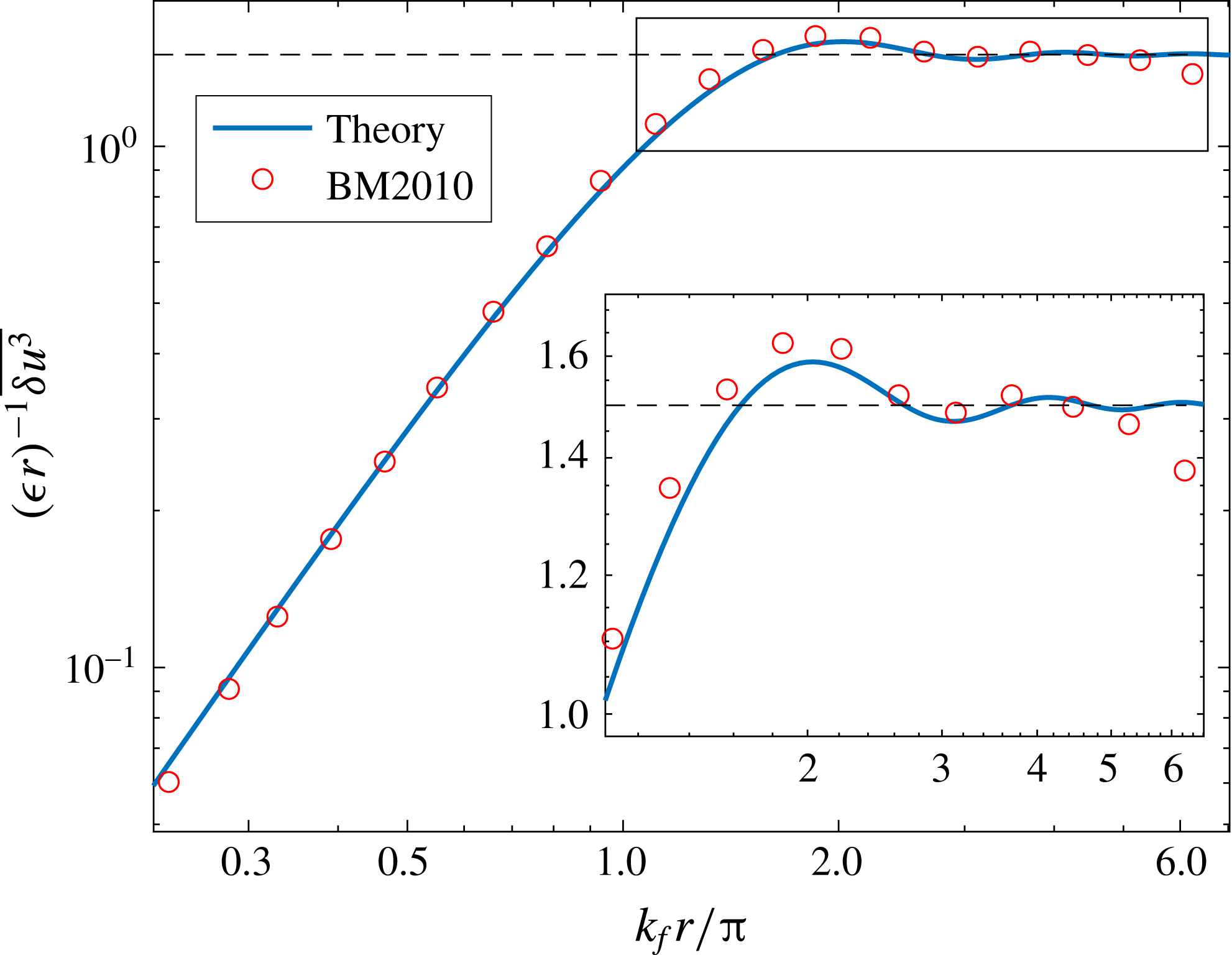
The plan of the paper is as follows. The governing equations and the main parts of the structure function relations are presented in § 2, which also includes a short self-contained account of Kolmogorov’s three-dimensional derivation. The two-dimensional situation is explored in § 3 for small and large scales, recovering (1.2) and suggesting robust diagnostic formulas. The exact expressions in the full non-dissipative range are explored in § 4 with special emphasis on the white noise in time case and comparison with numerical simulations in figure 1. The spectral energy transfer theory is summarized in § 5 and compared in some test cases against the much simpler robust diagnostics derived before. Concluding remarks are offered in § 6.
2 Governing equations and the Kármán–Howarth–Monin relation
We consider forced–dissipative incompressible flow in an unbounded domain described by
 $$\begin{eqnarray}\frac{\text{D}\boldsymbol{u}}{\text{D}t}+\unicode[STIX]{x1D735}p=-\unicode[STIX]{x1D6FC}\boldsymbol{u}+\unicode[STIX]{x1D708}\unicode[STIX]{x1D6FB}^{2}\boldsymbol{u}+\boldsymbol{F}\quad \text{and}\quad \unicode[STIX]{x1D735}\boldsymbol{\cdot }\boldsymbol{u}=0.\end{eqnarray}$$
Here
 $\boldsymbol{u}$
is the velocity vector,
 $\text{D}/\text{D}t=\unicode[STIX]{x2202}_{t}+(\boldsymbol{u}\boldsymbol{\cdot }\unicode[STIX]{x1D735})$
is the material derivative, the uniform density has been absorbed in the pressure
 $p$
and
 $\boldsymbol{F}$
is a random body force. Scale-selective dissipation is provided by Rayleigh friction with damping rate
 $\unicode[STIX]{x1D6FC}>0$
and Navier–Stokes diffusion with kinematic viscosity
 $\unicode[STIX]{x1D708}>0$
. The random force
 $\boldsymbol{F}$
has zero mean and is homogeneous in space and stationary in time and therefore
 $$\begin{eqnarray}\overline{\boldsymbol{F}(\boldsymbol{x},t)}=0\quad \text{and}\quad \overline{\boldsymbol{F}(\boldsymbol{x}_{1},t_{1})\boldsymbol{\cdot }\boldsymbol{F}(\boldsymbol{x}_{2},t_{2})}=R(\boldsymbol{x}_{2}-\boldsymbol{x}_{1},t_{2}-t_{1})\end{eqnarray}$$
hold for a suitable space–time covariance function
 $R$
. The overbar denotes statistical expectation. The ensuing random turbulent flow has zero mean component (i.e.
 $\overline{\boldsymbol{u}}=0$
) and is homogeneous in space as well. This implies that the covariance
 $$\begin{eqnarray}\overline{\boldsymbol{u}(\boldsymbol{x}_{1},t)\boldsymbol{\cdot }\boldsymbol{u}(\boldsymbol{x}_{2},t)}=\overline{\boldsymbol{u}_{1}\boldsymbol{\cdot }\boldsymbol{u}_{2}}\end{eqnarray}$$
depends only on the separation vector
 $\boldsymbol{x}=\boldsymbol{x}_{2}-\boldsymbol{x}_{1}$
. By construction, gradients of any mean field with respect to
 $(\boldsymbol{x},\boldsymbol{x}_{1},\boldsymbol{x}_{2})$
obey
 $$\begin{eqnarray}\unicode[STIX]{x1D735}=-\unicode[STIX]{x1D735}_{1}=\unicode[STIX]{x1D735}_{2}.\end{eqnarray}$$
Now, evaluating the governing equations at
 $\boldsymbol{x}_{1}$
and
 $\boldsymbol{x}_{2}$
, cross-multiplying, adding, averaging and following a number of calculus steps (e.g. Monin & Yaglom Reference Monin and Yaglom1975; Frisch Reference Frisch1995; Augier, Galtier & Billant Reference Augier, Galtier and Billant2012) yields the celebrated Kármán–Howarth–Monin (KHM) relation
 $$\begin{eqnarray}\frac{1}{2}\frac{\unicode[STIX]{x2202}\overline{(\boldsymbol{u}_{1}\boldsymbol{\cdot }\boldsymbol{u}_{2})}}{\unicode[STIX]{x2202}t}-\frac{1}{4}\unicode[STIX]{x1D735}\boldsymbol{\cdot }\boldsymbol{V}=(-\unicode[STIX]{x1D6FC}+\unicode[STIX]{x1D708}\unicode[STIX]{x1D6FB}^{2})\overline{\boldsymbol{u}_{1}\boldsymbol{\cdot }\boldsymbol{u}_{2}}+P.\end{eqnarray}$$
The independent variables in this exact statistical equation are the separation vector
 $\boldsymbol{x}$
and time
 $t$
. The power input term is
 $$\begin{eqnarray}P(\boldsymbol{x},t)={\textstyle \frac{1}{2}}\left(\overline{\boldsymbol{u}_{1}\boldsymbol{\cdot }\boldsymbol{F}_{2}}+\overline{\boldsymbol{F}_{1}\boldsymbol{\cdot }\boldsymbol{u}_{2}}\right)\end{eqnarray}$$
and
 $$\begin{eqnarray}P(0,t)=\overline{\boldsymbol{u}\boldsymbol{\cdot }\boldsymbol{F}}=\unicode[STIX]{x1D716}\end{eqnarray}$$
defines
 $\unicode[STIX]{x1D716}$
as the mean energy input due to
 $\boldsymbol{F}$
per unit time. The third-order structure function vector
 $\boldsymbol{V}$
is
 $$\begin{eqnarray}\boldsymbol{V}(\boldsymbol{x},t)=\overline{\left.|\unicode[STIX]{x1D6FF}\boldsymbol{u}|^{2}\,\unicode[STIX]{x1D6FF}\boldsymbol{u}\right.},\quad \text{where }\unicode[STIX]{x1D6FF}\boldsymbol{u}=\boldsymbol{u}_{2}-\boldsymbol{u}_{1}\end{eqnarray}$$
is the velocity difference between
 $\boldsymbol{x}_{2}$
and
 $\boldsymbol{x}_{1}$
. Second-order structure functions and correlations are related for any variable
 $A$
by
 $$\begin{eqnarray}\overline{\unicode[STIX]{x1D6FF}A^{2}}=2(\overline{A^{2}}-\overline{A_{1}A_{2}})\Rightarrow \unicode[STIX]{x1D735}\overline{\unicode[STIX]{x1D6FF}A^{2}}=-2\unicode[STIX]{x1D735}\overline{A_{1}A_{2}}.\end{eqnarray}$$
Only spatial homogeneity has been assumed to derive the KHM relation (2.5), which therefore holds in non-isotropic random flows as well. For stationary flows the mean fields are time independent and the steady KHM relation is
 $$\begin{eqnarray}\unicode[STIX]{x1D735}\boldsymbol{\cdot }\boldsymbol{V}=4\left(\unicode[STIX]{x1D6FC}-\unicode[STIX]{x1D708}\unicode[STIX]{x1D6FB}^{2}\right)\overline{\boldsymbol{u}_{1}\boldsymbol{\cdot }\boldsymbol{u}_{2}}-4P=4\left(\unicode[STIX]{x1D6FC}\,\overline{\boldsymbol{u}_{1}\boldsymbol{\cdot }\boldsymbol{u}_{2}}+\unicode[STIX]{x1D708}\,\overline{\unicode[STIX]{x1D74E}_{1}\boldsymbol{\cdot }\unicode[STIX]{x1D74E}_{2}}\right)-4P.\end{eqnarray}$$
The second form uses the covariance of the vorticity
 $\unicode[STIX]{x1D74E}=\unicode[STIX]{x1D735}\times \boldsymbol{u}$
, which for incompressible flow is linked to the velocity covariance by the remarkable identity (e.g. §11.3 in Monin & Yaglom (Reference Monin and Yaglom1975), Batchelor (Reference Batchelor1953))
 $$\begin{eqnarray}-\unicode[STIX]{x1D6FB}^{2}\,\overline{\boldsymbol{u}_{1}\boldsymbol{\cdot }\boldsymbol{u}_{2}}=\overline{\unicode[STIX]{x1D74E}_{1}\boldsymbol{\cdot }\unicode[STIX]{x1D74E}_{2}}.\end{eqnarray}$$
At zero separation
 $r=0$
the steady KHM relation reduces to the total energy balance
 $$\begin{eqnarray}\unicode[STIX]{x1D6FC}\overline{|\boldsymbol{u}|^{2}}+\unicode[STIX]{x1D708}\overline{|\unicode[STIX]{x1D74E}|^{2}}=P(0)=\unicode[STIX]{x1D716}.\end{eqnarray}$$
Finally, if the flow is isotropic then there exists a function
 $V(r)$
of the separation distance
 $r=|\boldsymbol{x}|$
such that
 $$\begin{eqnarray}\boldsymbol{V}=V(r)\,\widehat{\boldsymbol{r}}\quad \text{where }\widehat{\boldsymbol{r}}=\frac{\boldsymbol{x}}{r}.\end{eqnarray}$$
Hence
 $\unicode[STIX]{x1D735}\times \boldsymbol{V}=0$
for isotropic flows. If the flow is isotropic in
 $n$
spatial dimensions then
 $$\begin{eqnarray}V(r)=S_{L}(r)+(n-1)\,S_{T}(r)\end{eqnarray}$$
where the longitudinal and transversal structure functions are
 $$\begin{eqnarray}S_{L}=\overline{\unicode[STIX]{x1D6FF}u_{L}\unicode[STIX]{x1D6FF}u_{L}\unicode[STIX]{x1D6FF}u_{L}}\quad \text{and}\quad S_{T}=\overline{\unicode[STIX]{x1D6FF}u_{L}\,\unicode[STIX]{x1D6FF}u_{T}\unicode[STIX]{x1D6FF}u_{T}}.\end{eqnarray}$$
Here
 $\unicode[STIX]{x1D6FF}u_{L}=\widehat{\boldsymbol{r}}\boldsymbol{\cdot }\unicode[STIX]{x1D6FF}\boldsymbol{u}$
is the velocity difference component tangential to the separation vector and
 $\unicode[STIX]{x1D6FF}u_{T}$
is a component transversal to it.
2.1 Kolmogorov’s 4/5th law for three-dimensional isotropic turbulence
Kolmogorov’s 4/5th inertial range law for three-dimensional isotropic turbulence (without Rayleigh friction) follows from the first part of (2.10) with
 $\unicode[STIX]{x1D6FC}=0$
:
 $$\begin{eqnarray}\frac{1}{r^{2}}\frac{\text{d}}{\text{d}r}\left(r^{2}V\right)=2\unicode[STIX]{x1D708}\unicode[STIX]{x1D6FB}^{2}\,\overline{|\unicode[STIX]{x1D6FF}\boldsymbol{u}|^{2}}-4P(r).\end{eqnarray}$$
Here (2.9) was used for the viscous term. With
 $V(0)=0$
this is solved by
 $$\begin{eqnarray}V(r)=2\frac{\text{d}}{\text{d}r}\left(\unicode[STIX]{x1D708}\,\overline{|\unicode[STIX]{x1D6FF}\boldsymbol{u}|^{2}}\right)-\frac{4}{r^{2}}\int _{0}^{r}P(s)s^{2}\,\text{d}s.\end{eqnarray}$$
For high Reynolds numbers the viscous term in (2.17) is important only in the dissipation range
 $r\leqslant \ell _{\unicode[STIX]{x1D708}}=(\unicode[STIX]{x1D708}^{3}/\unicode[STIX]{x1D716})^{1/4}$
. Standard estimates put its relative size outside this range at
 $(\ell _{\unicode[STIX]{x1D708}}/r)^{4/3}$
(e.g. Landau & Lifshitz Reference Landau and Lifshitz1959; Frisch Reference Frisch1995). Conversely, if
 $r\ll \ell _{f}$
, where
 $\ell _{f}$
is the scale on which the force
 $\boldsymbol{F}$
supplies energy to the flow, then
 $P(r)$
is well approximated by its limiting value
 $P(0)=\unicode[STIX]{x1D716}$
. This yields Kolmogorov’s celebrated inertial range law
 $$\begin{eqnarray}\ell _{\unicode[STIX]{x1D708}}\ll r\ll \ell _{f}:\quad V(r)=-{\textstyle \frac{4}{3}}\unicode[STIX]{x1D716}r\Leftrightarrow S_{L}(r)=-{\textstyle \frac{4}{5}}\unicode[STIX]{x1D716}r\quad \text{and}\quad S_{T}(r)=-{\textstyle \frac{4}{15}}\unicode[STIX]{x1D716}r.\end{eqnarray}$$
This uses
 $S_{L}(0)=0$
and the three-dimensional isotropic relations
 $$\begin{eqnarray}V(r)=S_{L}(r)+2S_{T}(r)=S_{L}+\frac{1}{3}\frac{\text{d}}{\text{d}r}(rS_{L})=\frac{1}{3r^{3}}\frac{\text{d}}{\text{d}r}(r^{4}S_{L}).\end{eqnarray}$$
2.2 Importance of anomalous energy dissipation
The ease with which Kolmogorov’s law could be derived from (2.16) masks the crucial importance of anomalous energy dissipation for the analysis. Anomalous energy dissipation in three-dimensional turbulence means that
 $\unicode[STIX]{x1D708}\overline{|\unicode[STIX]{x1D74E}|^{2}}=\unicode[STIX]{x1D716}$
holds as
 $\unicode[STIX]{x1D708}\rightarrow 0$
, implying the familiar divergence of enstrophy as
 $1/\unicode[STIX]{x1D708}$
in the same limit. This can interfere with Taylor expanding the covariances for small
 $r$
. For example, using the second part of (2.10) instead of the first part gives the, still exact, equation
 $$\begin{eqnarray}\unicode[STIX]{x1D735}\boldsymbol{\cdot }\boldsymbol{V}=4\unicode[STIX]{x1D708}\overline{\unicode[STIX]{x1D74E}_{1}\boldsymbol{\cdot }\unicode[STIX]{x1D74E}_{2}}-4P=-2\unicode[STIX]{x1D708}\overline{|\unicode[STIX]{x1D6FF}\unicode[STIX]{x1D74E}|^{2}}+4(\unicode[STIX]{x1D708}\overline{|\unicode[STIX]{x1D74E}|^{2}}-P)=-2\unicode[STIX]{x1D708}\overline{|\unicode[STIX]{x1D6FF}\unicode[STIX]{x1D74E}|^{2}}+4(\unicode[STIX]{x1D716}-P).\end{eqnarray}$$
The previously used approximation
 $P(r)\approx \unicode[STIX]{x1D716}$
for small
 $r\ll \ell _{f}$
now yields a cancellation of constant terms on the right-hand side in (2.20), leaving behind only the enigmatic term
 $-2\unicode[STIX]{x1D708}\overline{|\unicode[STIX]{x1D6FF}\unicode[STIX]{x1D74E}|^{2}}$
, which in the inertial range is not small if
 $\unicode[STIX]{x1D708}\rightarrow 0$
. For example, a Taylor expansion of this term for small
 $r$
does not survive the limit
 $\unicode[STIX]{x1D708}\rightarrow 0$
. This is because the first term in such an expansion would be proportional to
 $\unicode[STIX]{x1D708}r^{2}\overline{|\unicode[STIX]{x1D735}\unicode[STIX]{x1D74E}|^{2}}$
, but according to standard scaling
 $\overline{|\unicode[STIX]{x1D735}\unicode[STIX]{x1D74E}|^{2}}\propto \unicode[STIX]{x1D716}^{3/2}/\unicode[STIX]{x1D708}^{5/2}$
, and hence if
 $\unicode[STIX]{x1D708}\rightarrow 0$
at fixed
 $r$
then
 $\unicode[STIX]{x1D708}r^{2}\overline{|\unicode[STIX]{x1D735}\unicode[STIX]{x1D74E}|^{2}}$
diverges as
 $\unicode[STIX]{x1D708}^{-3/2}$
, indicating a loss of smoothness in this limit. Hence, the approach based on the second part of (2.10) does not work in the three-dimensional case without further assumptions. However, precisely the same approach is the key for a successful analysis of the two-dimensional case, where the capricious vorticity gradient variance is bounded a priori.
3 Third-order structure functions for two-dimensional turbulence
Two-dimensional turbulence is very different from three-dimensional turbulence because of the absence of vortex stretching in the two-dimensional vorticity equation
 $$\begin{eqnarray}\frac{\text{D}\unicode[STIX]{x1D714}}{\text{D}t}=-\unicode[STIX]{x1D6FC}\unicode[STIX]{x1D714}+\unicode[STIX]{x1D708}\unicode[STIX]{x1D6FB}^{2}\unicode[STIX]{x1D714}+\unicode[STIX]{x1D735}\times \boldsymbol{F},\quad \text{where }\unicode[STIX]{x1D714}=\unicode[STIX]{x1D735}\times \boldsymbol{u}\end{eqnarray}$$
and
 $\unicode[STIX]{x1D735}\times$
from now on is shorthand for the vertical component of the curl. For small
 $(\unicode[STIX]{x1D6FC},\unicode[STIX]{x1D708})$
, enstrophy with density
 $\unicode[STIX]{x1D714}^{2}/2$
is predominantly dissipated at small scales
 $r\ll \ell _{f}$
whereas energy with density
 $|\boldsymbol{u}|^{2}/2$
is predominantly dissipated at large scales
 $r\gg \ell _{f}$
. Hence, as
 $\unicode[STIX]{x1D708}\rightarrow 0$
anomalous small-scale dissipation applies to enstrophy, not to energy.
The identity (2.11) means that applying
 $-\unicode[STIX]{x1D6FB}^{2}$
to the KHM relation (2.5) yields the evolution equation for
 $\overline{\unicode[STIX]{x1D714}_{1}\unicode[STIX]{x1D714}_{2}}/2$
, with
 $-\unicode[STIX]{x1D6FB}^{2}P$
emerging as the forcing term for the enstrophy. At
 $r=0$
the total energy balance
 $$\begin{eqnarray}\unicode[STIX]{x1D6FC}\overline{|\boldsymbol{u}|^{2}}+\unicode[STIX]{x1D708}\overline{\unicode[STIX]{x1D714}^{2}}=P(0)=\unicode[STIX]{x1D716}\end{eqnarray}$$
is now paired with the analogous total enstrophy balance
 $$\begin{eqnarray}\unicode[STIX]{x1D6FC}\overline{\unicode[STIX]{x1D714}^{2}}+\unicode[STIX]{x1D708}\overline{|\unicode[STIX]{x1D735}\unicode[STIX]{x1D714}|^{2}}=-\unicode[STIX]{x1D6FB}^{2}P(0)=\unicode[STIX]{x1D702}.\end{eqnarray}$$
This defines
 $\unicode[STIX]{x1D702}$
as the mean enstrophy input due to
 $\boldsymbol{F}$
per unit time. Using (3.2) in the two-dimensional steady KHM relation yields
 $$\begin{eqnarray}\frac{1}{r}\frac{\text{d}}{\text{d}r}(rV)=-2(\unicode[STIX]{x1D6FC}\overline{|\unicode[STIX]{x1D6FF}\boldsymbol{u}|^{2}}+\unicode[STIX]{x1D708}\overline{\unicode[STIX]{x1D6FF}\unicode[STIX]{x1D714}^{2}})+4(\unicode[STIX]{x1D716}-P).\end{eqnarray}$$
Note the similarity with (2.20) in three-dimensional turbulence. However, in two dimensions the dissipation terms in (3.4) are now bounded and smooth for all values of
 $r$
. This is because
 $\unicode[STIX]{x1D708}\overline{|\unicode[STIX]{x1D735}\unicode[STIX]{x1D714}|^{2}}$
is now bounded a priori by the two-dimensional enstrophy balance (3.3), which implies that
 $\overline{\unicode[STIX]{x1D6FF}\unicode[STIX]{x1D714}^{2}}=O(r^{2})$
for small
 $r\ll \ell _{f}$
. Integrating (3.4) from zero with
 $V(0)=0$
yields
 $$\begin{eqnarray}V(r)=-\frac{1}{r}\int _{0}^{r}2(\unicode[STIX]{x1D6FC}\overline{|\unicode[STIX]{x1D6FF}\boldsymbol{u}|^{2}}+\unicode[STIX]{x1D708}\overline{\unicode[STIX]{x1D6FF}\unicode[STIX]{x1D714}^{2}})s\,\text{d}s+2\unicode[STIX]{x1D716}r-\frac{4}{r}\int _{0}^{r}P(s)s\,\text{d}s.\end{eqnarray}$$
3.1 Small-scale asymptotics in the enstrophy inertial range
For small
 $r\ll \ell _{f}$
the one-term approximation
 $P(r)\approx \unicode[STIX]{x1D716}$
now merely leads to a cancellation between the last two terms in (3.5), hence we now consider the two-term expansion
 $$\begin{eqnarray}P(r)=\unicode[STIX]{x1D716}-\frac{\unicode[STIX]{x1D702}}{4}r^{2}+O(r^{4}),\end{eqnarray}$$
which uses the definition of
 $\unicode[STIX]{x1D702}$
in (3.3) and that
 $\unicode[STIX]{x1D6FB}^{2}r^{2}=4$
in two dimensions. This yields
 $$\begin{eqnarray}r\ll \ell _{f}:\quad V(r)=-\frac{C(r)}{r}+\frac{1}{4}\unicode[STIX]{x1D702}r^{3},\end{eqnarray}$$
where we used the shorthand
 $C(r)\geqslant 0$
for the dissipation integral. It is interesting to compare (3.7) with its three-dimensional counterpart (2.17). In both cases
 $V(r)$
contains a dissipation term and a flux term. The three-dimensional dissipation term is local in
 $r$
and in the inertial range it can be readily ignored, as stated before. The two-dimensional dissipation term is non-local in
 $r$
and contains a sign-definite integral
 $C(r)\geqslant 0$
that accumulates contributions from all scales less than
 $r$
, which includes the dissipation range. To estimate the size
 $C(r)\geqslant 0$
we consider separately its contribution from the dissipation and from the inertial range. With slight abuse of notation the two-dimensional dissipation range is again
 $r\leqslant \ell _{\unicode[STIX]{x1D708}}$
with a new
 $\ell _{\unicode[STIX]{x1D708}}=\sqrt{\unicode[STIX]{x1D708}/\unicode[STIX]{x1D702}^{1/3}}$
. The dissipation range integral must cancel the
 $\unicode[STIX]{x1D702}r^{3}/4$
flux term and therefore we can estimate
 $C(\ell _{\unicode[STIX]{x1D708}})=\unicode[STIX]{x1D702}\ell _{\unicode[STIX]{x1D708}}^{4}/4$
. The relative size of
 $C(\ell _{\unicode[STIX]{x1D708}})/r$
compared to the flux term is then
 $(\ell _{\unicode[STIX]{x1D708}}/r)^{4}$
, which is indeed very small in the inertial range.
To estimate the inertial range contribution to
 $C(r)$
we use the inertial range scalings
 $\overline{|\unicode[STIX]{x1D6FF}\boldsymbol{u}|^{2}}\propto \unicode[STIX]{x1D702}^{2/3}r^{2}$
and
 $\overline{\unicode[STIX]{x1D6FF}\unicode[STIX]{x1D714}^{2}}\propto \unicode[STIX]{x1D702}^{2/3}$
, which are based on dimensional analysis. The inertial range contribution to
 $C(r)/r$
of the damping term then scales as
 $\unicode[STIX]{x1D6FC}\unicode[STIX]{x1D702}^{2/3}r^{3}$
and that of the viscous term scales as
 $\unicode[STIX]{x1D708}\unicode[STIX]{x1D702}^{2/3}r$
. Their relative magnitudes compared to the flux term are then
 $\unicode[STIX]{x1D6FC}/\unicode[STIX]{x1D702}^{1/3}$
and
 $(\ell _{\unicode[STIX]{x1D708}}/r)^{2}$
, respectively. Notably, the former does not depend on
 $r$
. In summary, the viscous term in (3.7) is irrelevant in the inertial range, as compared to the flux term both contributions to it vanish rapidly with
 $(\ell _{\unicode[STIX]{x1D708}}/r)^{4}$
and
 $(\ell _{\unicode[STIX]{x1D708}}/r)^{2}$
. The damping term is irrelevant if
 $$\begin{eqnarray}\unicode[STIX]{x1D6FC}\ll \unicode[STIX]{x1D702}^{1/3},\end{eqnarray}$$
which is a natural physical condition for weak damping, which leaves the flux of enstrophy through the inertial range intact. Overall, in the small-scale enstrophy flux range of two-dimensional turbulence this analogue of (2.18) holds (Lindborg Reference Lindborg1999):
 $$\begin{eqnarray}\ell _{\unicode[STIX]{x1D708}}\ll r\ll \ell _{f}:\quad V(r)={\textstyle \frac{1}{4}}\unicode[STIX]{x1D702}r^{3}\Leftrightarrow S_{L}(r)=S_{T}(r)={\textstyle \frac{1}{8}}\unicode[STIX]{x1D702}r^{3}.\end{eqnarray}$$
This uses the two-dimensional counterpart of (2.19), which is (e.g. Lindborg Reference Lindborg1999)
 $$\begin{eqnarray}V(r)=S_{L}(r)+S_{T}(r)=S_{L}+\frac{r}{3}\frac{\text{d}}{\text{d}r}(S_{L})=\frac{1}{3r^{2}}\frac{\text{d}}{\text{d}r}(r^{3}S_{L}).\end{eqnarray}$$
Actually, the expressions for
 $S_{L}$
and
 $S_{T}$
in (3.9) are slight approximations to the exact
 $$\begin{eqnarray}S_{L}(r)=\frac{3}{r^{3}}\,\int _{0}^{r}V(s)s^{2}\,\text{d}s\quad \text{and}\quad S_{T}(r)=V(r)-S_{L}(r).\end{eqnarray}$$
For example, if the power law for
 $V(r)$
changes with
 $r$
then the structure functions adjust to the new power law with an error that decays rapidly with
 $1/r^{3}$
. This small error will be ignored from now on.
3.2 Large-scale asymptotics in the energy inertial range
At scales
 $r\gg \ell _{f}$
larger than the forcing scale the downscale enstrophy flux is replaced by an upscale energy flux, and
 $2\unicode[STIX]{x1D716}r$
becomes important in (3.5). However, as noted in the introduction, there is no universal asymptotic behaviour for the function
 $P(r)$
at large scales. This will be illustrated in § 4.2, but for the moment we note that the commonly made (e.g. Lindborg Reference Lindborg1999) approximation
 $P(r)\approx 0$
for
 $r>\ell _{f}$
leads to
 $$\begin{eqnarray}\ell _{f}\ll r:\quad V(r)=-\frac{C(r)}{r}+2\unicode[STIX]{x1D716}r-\frac{D}{r}.\end{eqnarray}$$
Here
 $D$
is the integral of
 $4P(s)s$
from zero to
 $r=\ell _{f}$
. The dissipation term
 $-C(r)/r$
can be estimated using the standard dimensional scaling relations
 $\overline{|\unicode[STIX]{x1D6FF}\boldsymbol{u}|^{2}}\propto (\unicode[STIX]{x1D716}r)^{2/3}$
and
 $\overline{\unicode[STIX]{x1D6FF}\unicode[STIX]{x1D714}^{2}}\propto \unicode[STIX]{x1D716}^{1/3}r^{-2/3}$
. For the damping and viscous terms this leads to the scaling estimates
 $\unicode[STIX]{x1D6FC}\unicode[STIX]{x1D716}^{2/3}r^{5/3}$
and
 $\unicode[STIX]{x1D708}\unicode[STIX]{x1D716}^{2/3}r^{-1/3}$
, respectively. The latter is ignorable throughout, but the former becomes comparable to the
 $\unicode[STIX]{x1D716}r$
term at the large-scale damping scale
 $\ell _{\unicode[STIX]{x1D6FC}}=\unicode[STIX]{x1D716}^{1/2}\unicode[STIX]{x1D6FC}^{-3/2}$
. This leads to the energy inertial range flux relations
 $$\begin{eqnarray}\ell _{f}\ll r\ll \ell _{\unicode[STIX]{x1D6FC}}:\quad V(r)=2\unicode[STIX]{x1D716}r-\frac{D}{r}\Leftrightarrow S_{L}(r)=\frac{3}{2}\unicode[STIX]{x1D716}r-\frac{3}{2}\frac{D}{r},\quad S_{T}(r)=\frac{1}{2}\unicode[STIX]{x1D716}r+\frac{1}{2}\frac{D}{r}\end{eqnarray}$$
although the
 $D/r$
terms are usually ignored (Lindborg Reference Lindborg1999). As discussed before, these power-law expressions for
 $S_{L}(r)$
and
 $S_{T}(r)$
ignore higher-order corrections proportional to
 $1/r^{3}$
.
3.3 Robust diagnostics for energy and enstrophy fluxes
The prior asymptotic analysis of the KHM equation allows the estimation of
 $\unicode[STIX]{x1D716}$
and
 $\unicode[STIX]{x1D702}$
from observations of
 $S_{L}$
and
 $S_{T}$
. For example, the standard way to proceed in the estimation of
 $\unicode[STIX]{x1D716}$
is to plot the compensated structure functions
 $V/(2r)$
or
 $2S_{L}/(3r)$
, either of which should asymptote to
 $\unicode[STIX]{x1D716}$
in the energy inertial range. However, with both structure functions
 $S_{L}$
and
 $S_{T}$
at hand one can do better and arguably achieve more robust diagnostics. For example, if (3.13) is accurate then the
 $D/r$
term can be eliminated by using
 $$\begin{eqnarray}\unicode[STIX]{x1D716}=\frac{1}{3r}\left(S_{L}(r)+3S_{T}(r)\right)\end{eqnarray}$$
for estimating
 $\unicode[STIX]{x1D716}$
, say just above the forcing scale
 $r=\ell _{f}$
. Another perspective on (3.14) is that
 $V(r)$
as a solution of (3.4) in some finite range of
 $r$
consists of a local particular solution that balances the right-hand side plus a non-local homogeneous solution proportional to
 $1/r$
. The robust diagnostics above then eliminate the homogeneous part of the solution. More generally, if
 $$\begin{eqnarray}V(r)=r^{\,p}\quad \text{then }S_{L}(r)=\frac{3}{3+p}\,r^{\,p}\quad \text{and}\quad S_{T}(r)=\frac{p}{3+p}\,r^{\,p}.\end{eqnarray}$$
Hence an
 $r^{\,p}$
term is filtered by the linear combination
 $-pS_{L}+3S_{T}$
. Now, consider a hypothetical situation in which
 $$\begin{eqnarray}V(r)=2\unicode[STIX]{x1D716}_{1}r+{\textstyle \frac{1}{4}}\unicode[STIX]{x1D702}_{2}r^{3}\end{eqnarray}$$
held for some range in
 $r$
. Here
 $\unicode[STIX]{x1D716}_{1}$
and
 $\unicode[STIX]{x1D702}_{2}$
are related to different forcing mechanisms operating at scales
 $\ell _{1}\ll r\ll \ell _{2}$
, say. In other words,
 $r$
lies in the energy inertial range relative to the first forcing mechanism and in the enstrophy inertial range relative to the second forcing mechanism. Then the robust diagnostics
 $$\begin{eqnarray}\unicode[STIX]{x1D716}_{1}=\frac{1}{r}\left(S_{L}(r)-S_{T}(r)\right)\quad \text{and}\quad \unicode[STIX]{x1D702}_{2}=\frac{4}{r^{3}}\left(-S_{L}(r)+3S_{T}(r)\right)\end{eqnarray}$$
would exactly disentangle the energy and enstrophy fluxes. This will be illustrated in § 5.2 below.
4 Exact non-dissipative results
The small-scale and large-scale asymptotic expressions (3.9) and (3.13) are not valid across the forcing scale
 $r\approx \ell _{f}$
, which is a severe handicap in the practically important situation of forcing at more than one scale, and of measurements taken in ranges that overlap with the forcing. In this section we explore the exact result for
 $V(r)$
in (3.5) across the entire non-dissipative range
 $$\begin{eqnarray}\ell _{\unicode[STIX]{x1D708}}\ll r\ll \ell _{\unicode[STIX]{x1D6FC}}\quad \text{where }\ell _{\unicode[STIX]{x1D708}}=\frac{\unicode[STIX]{x1D708}^{1/2}}{\unicode[STIX]{x1D702}^{1/6}}\quad \text{and}\quad \ell _{\unicode[STIX]{x1D6FC}}=\frac{\unicode[STIX]{x1D716}^{1/2}}{\unicode[STIX]{x1D6FC}^{3/2}}.\end{eqnarray}$$
Here
 $\unicode[STIX]{x1D716}=P(0)$
and
 $\unicode[STIX]{x1D702}=-\unicode[STIX]{x1D6FB}^{2}P(0)$
are the total energy and enstrophy input rates as before, which involve the exact
 $P$
as defined in (2.6). In this non-dissipative range (3.5) reduces to
 $$\begin{eqnarray}\ell _{\unicode[STIX]{x1D708}}\ll r\ll \ell _{\unicode[STIX]{x1D6FC}}:\quad V(r)=2\unicode[STIX]{x1D716}r-\frac{4}{r}\int _{0}^{r}P(s)s\,\text{d}s\quad \text{and}\quad \unicode[STIX]{x1D735}\boldsymbol{\cdot }\boldsymbol{V}=4(\unicode[STIX]{x1D716}-P).\end{eqnarray}$$
The corresponding expressions for
 $S_{L}(r)$
and
 $S_{T}(r)$
follow from (3.10) as
 $$\begin{eqnarray}S_{L}(r)=\frac{3}{2}\unicode[STIX]{x1D716}r-\frac{6}{r}\int _{0}^{r}P(s)s\,\text{d}s+\frac{6}{r^{3}}\int _{0}^{r}P(s)s^{3}\,\text{d}s\end{eqnarray}$$
and
 $$\begin{eqnarray}S_{T}(r)=\frac{1}{2}\unicode[STIX]{x1D716}r+\frac{2}{r}\int _{0}^{r}P(s)\,s\,\text{d}s-\frac{6}{r^{3}}\int _{0}^{r}P(s)s^{3}\,\text{d}s.\end{eqnarray}$$
4.1 White noise in time forcing
In general,
 $P$
is not known a priori, i.e. it is part of the solution rather than the problem, because it depends both on the given random force
 $\boldsymbol{F}$
and on the unknown fluid velocity
 $\boldsymbol{u}$
induced by
 $\boldsymbol{F}$
. An important exception to this is the case of white noise in time forcing, in which the force covariance (2.2) is
 $$\begin{eqnarray}\overline{\boldsymbol{F}(\boldsymbol{x}_{1},t_{1})\boldsymbol{\cdot }\boldsymbol{F}(\boldsymbol{x}_{2},t_{2})}=R(\boldsymbol{x}_{2}-\boldsymbol{x}_{1})\unicode[STIX]{x1D6FF}(t_{2}-t_{1})=R(\boldsymbol{x})\unicode[STIX]{x1D6FF}(t_{2}-t_{1})\end{eqnarray}$$
with a smooth spatial covariance function
 $R(\boldsymbol{x})$
. Here we assumed
 $\unicode[STIX]{x1D735}\boldsymbol{\cdot }\boldsymbol{F}=0$
, as any divergent part of
 $\boldsymbol{F}$
is simply absorbed by the fluid pressure. As is well known (e.g. Bernard Reference Bernard1999; Srinivasan & Young Reference Srinivasan and Young2012), for this kind of forcing
 $$\begin{eqnarray}P(\boldsymbol{x})={\textstyle \frac{1}{2}}(\overline{\boldsymbol{u}_{1}\boldsymbol{\cdot }\boldsymbol{F}_{2}}+\overline{\boldsymbol{F}_{1}\boldsymbol{\cdot }\boldsymbol{u}_{2}})={\textstyle \frac{1}{2}}R(\boldsymbol{x})\end{eqnarray}$$
holds in the stationary regime (also for anisotropic flows). In other words, for white noise in time forcing the function
 $P(\boldsymbol{x})$
is known a priori from (4.6) and hence the third-order structure functions in the non-dissipative range can be read off from (4.2), without any need for an actual numerical simulation.
4.2 Structure function models and comparison with simulation
Many different covariance functions
 $P(r)$
are compatible with an energy input rate
 $P(0)=\unicode[STIX]{x1D716}$
at some scale
 $\ell _{f}$
, subject only to the usual condition that its Fourier transform
 $\hat{P}$
, say, is real and non-negative (e.g. Yaglom Reference Yaglom1962). We consider two common models for
 $P(r)$
to indicate the range of possibilities. The first model has a spatially localized covariance given by
 $$\begin{eqnarray}P_{1}(r)=\unicode[STIX]{x1D716}\exp \left(\frac{-r^{2}}{4\ell _{f}^{2}}\right),\end{eqnarray}$$
which means that
 $\hat{P}_{1}\propto \exp (-\unicode[STIX]{x1D705}^{2}\ell _{f}^{2})$
where
 $\unicode[STIX]{x1D705}=|\boldsymbol{k}|$
is the magnitude of the wavenumber vector
 $\boldsymbol{k}$
. This corresponds to forced wavenumbers that are concentrated in a neighbourhood of approximate size
 $1/\ell _{f}$
surrounding the origin
 $\boldsymbol{k}=0$
. The concomitant rapid decay of the spatial covariance function with
 $r$
makes this a reasonable model for spatially localized forces. In the second model
 $$\begin{eqnarray}P_{2}(r)=\unicode[STIX]{x1D716}\,\text{J}_{0}(r/\ell _{f}),\end{eqnarray}$$
where
 $\text{J}_{0}$
is a Bessel function. This corresponds to the often-used numerical method where only wavenumbers in a small neighbourhood of the ring
 $\unicode[STIX]{x1D705}=1/\ell _{f}$
are forced; equation (4.8) arises in the limit where the width of that neighbourhood shrinks to zero such that
 $\hat{P}_{2}\propto \unicode[STIX]{x1D6FF}(\unicode[STIX]{x1D705}-1/\ell _{f})$
. The perfect localization in spectral space comes at the price of long-range correlations in real space, which are not obviously a realistic feature for a physical process. It is easy to check that the enstrophy input rate
 $\unicode[STIX]{x1D702}=\unicode[STIX]{x1D716}/\ell _{f}^{2}$
for both (4.7) and (4.8), where the latter uses
 $\unicode[STIX]{x1D6FB}^{2}\text{J}_{0}=-\text{J}_{0}$
.
The functions
 $V(r)$
for the two models are found from (4.2) as
 $$\begin{eqnarray}V_{1}=2\unicode[STIX]{x1D716}r-8\unicode[STIX]{x1D716}\frac{\ell _{f}^{2}}{r}\left[1-\exp \left(\frac{-r^{2}}{4\ell _{f}^{2}}\right)\right]\quad \text{and}\quad V_{2}=2\unicode[STIX]{x1D716}r-4\unicode[STIX]{x1D716}\ell _{f}\,J_{1}(r/\ell _{f}).\end{eqnarray}$$
The corresponding longitudinal structure functions are
 $$\begin{eqnarray}S_{L1}=\frac{3}{2}\unicode[STIX]{x1D716}r-12\unicode[STIX]{x1D716}\frac{\ell _{f}^{2}}{r}+48\unicode[STIX]{x1D716}\frac{\ell _{f}^{4}}{r^{3}}\left[1-\exp \left(\frac{-r^{2}}{4\ell _{f}^{2}}\right)\right]\end{eqnarray}$$
and
 $$\begin{eqnarray}S_{L2}=\frac{3}{2}\unicode[STIX]{x1D716}r-12\unicode[STIX]{x1D716}\frac{\ell _{f}^{2}}{r}\,J_{2}(r/\ell _{f}).\end{eqnarray}$$
Their transverse counterparts follow from
 $S_{T}=V-S_{L}$
. Both
 $S_{L1}$
and
 $S_{L2}$
reduce to
 $\unicode[STIX]{x1D702}r^{3}/8$
and
 $3\unicode[STIX]{x1D716}r/2$
in the limits
 $r\ll \ell _{f}$
and
 $r\gg \ell _{f}$
, but the form of their transition between these generic limits is obviously very different. This provides a testable prediction of our theory.
In particular, the white-noise forcing (4.8) has been used in the numerical experiments of Boffetta & Musacchio (Reference Boffetta and Musacchio2010), which at their highest resolution captured both the small-scale and large-scale regimes and the transition between them. In figure 1 we compare the theoretical result (4.11) with the numerical data obtained by Boffetta & Musacchio (Reference Boffetta and Musacchio2010). This shows a remarkably accurate matching throughout the non-dissipative range, which includes the predicted Bessel-type oscillation.
Comparison of predicted
 $S_{L}$
from (4.11) (blue curve) with the data from figure 3 of Boffetta & Musacchio (Reference Boffetta and Musacchio2010) (red circles), where the associated high-resolution numerical simulation (run E) used
 $32768^{2}$
grid points. The axis labels have been chosen for easy comparison with Boffetta & Musacchio (Reference Boffetta and Musacchio2010). The horizontal dashed lines mark the constant
 $3/2$
, the inset enlarges the rectangular transition region and
 $k_{f}=1/\ell _{f}$
.

5 Spectral energy flux
The most precise measure of energy transfer across spatial scales is based on a Fourier transform of the KHM relation (e.g. Frisch Reference Frisch1995; Davidson Reference Davidson2015), which brings in the two-dimensional energy spectrum
 $$\begin{eqnarray}E(\boldsymbol{k},t)=\frac{1}{2}\widehat{\left.\overline{\boldsymbol{u}_{1}\boldsymbol{\cdot }\boldsymbol{u}_{2}}\right.}=\frac{1}{(2\unicode[STIX]{x03C0})^{2}}\int \frac{1}{2}\overline{\boldsymbol{u}_{1}\boldsymbol{\cdot }\boldsymbol{u}_{2}}\,\exp (-\text{i}\boldsymbol{k}\boldsymbol{\cdot }\boldsymbol{x})\,\text{d}x\,\text{d}y.\end{eqnarray}$$
By construction,
 $E$
is a real, even and non-negative function of
 $\boldsymbol{k}$
, and its total integral over
 $\boldsymbol{k}$
is the mean energy density. The transformed KHM relation is
 $$\begin{eqnarray}\frac{\unicode[STIX]{x2202}E}{\unicode[STIX]{x2202}t}-\frac{1}{4}\widehat{\unicode[STIX]{x1D735}\boldsymbol{\cdot }\boldsymbol{V}}=\hat{P}-2(\unicode[STIX]{x1D6FC}+\unicode[STIX]{x1D708}\unicode[STIX]{x1D705}^{2})E.\end{eqnarray}$$
On the right-hand side are the forcing and dissipation terms. In a stationary state any discrepancy between these terms must be balanced by the third-order term on the left, which stems from the nonlinear terms in the governing equations. The spectral energy budget is additive over disjoint subsets of
 $\boldsymbol{k}$
-space, so if
 ${\mathcal{D}}_{K}$
denotes any subset of
 $\boldsymbol{k}$
-space then
 $$\begin{eqnarray}\unicode[STIX]{x1D6F1}_{K}=\int _{{\mathcal{D}}_{K}}-\frac{1}{4}\widehat{\unicode[STIX]{x1D735}\boldsymbol{\cdot }\boldsymbol{V}}\,\text{d}k\,\text{d}l=\int _{{\mathcal{D}}_{K}}\left[\hat{P}-2(\unicode[STIX]{x1D6FC}+\unicode[STIX]{x1D708}\unicode[STIX]{x1D705}^{2})E-\frac{\unicode[STIX]{x2202}E}{\unicode[STIX]{x2202}t}\right]\,\text{d}k\,\text{d}l\end{eqnarray}$$
precisely measures the nonlinear energy flux leaving
 ${\mathcal{D}}_{K}$
. Of course, the term ‘flux’ is slightly misleading here, as
 $\unicode[STIX]{x1D6F1}_{K}$
is given by a bulk integral over
 ${\mathcal{D}}_{K}$
rather than a surface integral over its boundary. If
 $$\begin{eqnarray}{\mathcal{D}}_{K}=\left\{\boldsymbol{k}:\unicode[STIX]{x1D705}=|\boldsymbol{k}|\leqslant K\right\}\end{eqnarray}$$
is a circular region then the energy flux
 $$\begin{eqnarray}\unicode[STIX]{x1D6F1}_{K}=\int -\frac{1}{4}\widehat{\unicode[STIX]{x1D735}\boldsymbol{\cdot }\boldsymbol{V}}H(K-\unicode[STIX]{x1D705})\,\text{d}k\,\text{d}l=-\frac{1}{8\unicode[STIX]{x03C0}}\int \unicode[STIX]{x1D735}\boldsymbol{\cdot }\boldsymbol{V}\,\frac{K}{r}J_{1}(Kr)\,\text{d}x\,\text{d}y.\end{eqnarray}$$
Here
 $H(\cdot )$
is the Heaviside function and the second form uses Plancherel’s theorem.
5.1 Computation of energy and enstrophy fluxes
One way to compute
 $\unicode[STIX]{x1D6F1}_{K}$
is by substituting for
 $\unicode[STIX]{x1D735}\boldsymbol{\cdot }\boldsymbol{V}$
or its Fourier transform from the steady balance in (3.4), or from its non-dissipative approximation (4.2). For example, equations (4.7) and (4.8) would lead to the exact spectral energy fluxes
 $$\begin{eqnarray}\unicode[STIX]{x1D6F1}_{K1}=-\unicode[STIX]{x1D716}\exp (-K^{2}\ell _{f}^{2})\quad \text{and}\quad \unicode[STIX]{x1D6F1}_{K2}=-\unicode[STIX]{x1D716}(1-H(K\ell _{f}-1))\end{eqnarray}$$
for
 $K$
in the non-dissipative wavenumber range. Conversely, equation (5.5) can be used directly if
 $V$
is measured in an experiment. In this case it is crucial to integrate by parts in order to avoid derivatives of the noisy field
 $V$
, which yields
 $$\begin{eqnarray}\unicode[STIX]{x1D6F1}_{K}=-\frac{1}{8\unicode[STIX]{x03C0}}\int (\boldsymbol{V}\boldsymbol{\cdot }\widehat{\boldsymbol{r}})\frac{K^{2}}{r}J_{2}(Kr)\,\text{d}x\,\text{d}y.\end{eqnarray}$$
So far we have not assumed isotropy, but with that assumption
 $\boldsymbol{V}\boldsymbol{\cdot }\widehat{\boldsymbol{r}}=V(r)$
and hence
 $$\begin{eqnarray}\unicode[STIX]{x1D6F1}_{K}=-\frac{K^{2}}{4}\int _{0}^{\infty }V(r)J_{2}(Kr)\,\text{d}r=-\frac{K^{3}}{12}\int _{0}^{\infty }S_{L}(r)J_{3}(Kr)r\,\text{d}r,\end{eqnarray}$$
where (3.10) has been used. These are exact relations, although in practice their utility is limited by the accuracy and range of the observed
 $V(r)$
. It is not difficult to check that substituting the generic
 $V=2\unicode[STIX]{x1D716}r$
into (5.8) yields
 $\unicode[STIX]{x1D6F1}_{K}=-\unicode[STIX]{x1D716}$
, a negative flux consistent with the inverse energy flux.
Based on (2.11) a corresponding spectral enstrophy flux
 $\unicode[STIX]{x1D6F1}_{K}^{\unicode[STIX]{x1D714}}$
, say, can be constructed provided that
 $\unicode[STIX]{x1D735}\boldsymbol{\cdot }\boldsymbol{V}$
is replaced by
 $-\unicode[STIX]{x1D6FB}^{2}\unicode[STIX]{x1D735}\boldsymbol{\cdot }\boldsymbol{V}$
. Mutatis mutandis, for the white-noise examples this leads to the exact enstrophy fluxes
 $$\begin{eqnarray}\unicode[STIX]{x1D6F1}_{K1}^{\unicode[STIX]{x1D714}}=\unicode[STIX]{x1D702}(1-(K^{2}\ell _{f}^{2}+1)\text{e}^{-K^{2}\ell _{f}^{2}})\quad \text{and}\quad \unicode[STIX]{x1D6F1}_{K2}^{\unicode[STIX]{x1D714}}=\unicode[STIX]{x1D702}\,H(K\ell _{f}-1)\end{eqnarray}$$
in the non-dissipative range. As (5.6) and (5.9) are not valid for
 $K$
in the large-scale or small-scale dissipation ranges, they do not satisfy the global constraints noted in § 10.3.4 of Davidson (Reference Davidson2015).
5.2 Test of robust energy flux diagnostics
The spectral flux diagnostics displayed in the last section are the most precise measures of scale-to-scale energy transfer, but, as exemplified by (5.8), for each
 $K$
they rely on integrals of
 $V(r)$
over all
 $r$
. In practice, it is therefore valuable to have simpler diagnostics that only use the structure functions in some local range of
 $r$
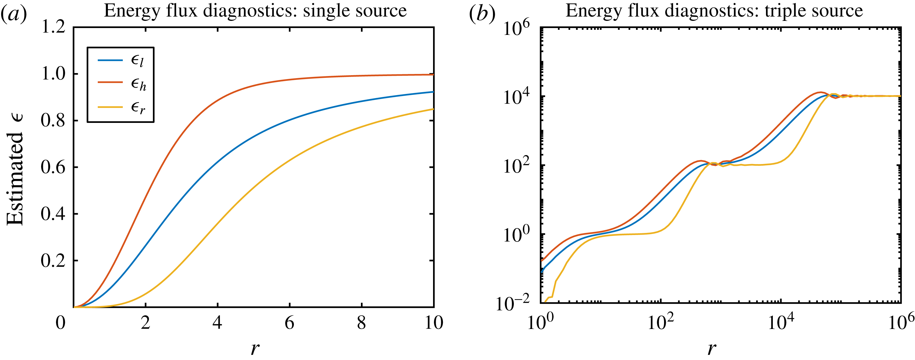
. Here we test the robust energy flux diagnostics proposed in § 3.3 using two examples illustrated in figure 2. In the first example there is a single energy source of type (4.7) with
 $\unicode[STIX]{x1D716}=1$
and
 $\ell _{f}=1$
and the following three energy flux diagnostics are compared in figure 2(a):
 $$\begin{eqnarray}\unicode[STIX]{x1D716}_{l}=\frac{2}{3r}S_{L},\quad \unicode[STIX]{x1D716}_{h}=\frac{S_{L}+3S_{T}}{3r},\quad \unicode[STIX]{x1D716}_{r}=\frac{S_{L}-S_{T}}{r}.\end{eqnarray}$$
Here
 $\unicode[STIX]{x1D716}_{l}$
is the standard estimate for
 $\unicode[STIX]{x1D716}$
based on the expression for
 $S_{L}$
in (3.13),
 $\unicode[STIX]{x1D716}_{h}$
is from (3.14), which filters the
 $1/r$
term, and
 $\unicode[STIX]{x1D716}_{r}$
is from (3.17) and filters the enstrophy flux
 $r^{3}$
term. Figure 2(a) shows that
 $\unicode[STIX]{x1D716}_{h}$
converges most quickly to
 $\unicode[STIX]{x1D716}=1$
as
 $r$
increases, as expected. The second example is more challenging: we add two further energy sources of type (4.8) to mimic three different energy sources with parameters
 $$\begin{eqnarray}\unicode[STIX]{x1D716}\in \{1,10^{2},10^{4}\}\quad \text{and}\quad \ell _{f}\in \{1,10^{2},10^{4}\}.\end{eqnarray}$$
Here the large-scale energy sources are strong enough such that their downscale enstrophy flux interferes with the upscale energy flux of the small-scale sources, which makes this a challenging problem. From (5.6), the exact spectral energy flux
 $$\begin{eqnarray}\unicode[STIX]{x1D6F1}_{K}=\,-\exp (-K^{2})-10^{2}(1-H(10^{2}K-1))-10^{4}(1-H(10^{4}K-1))\end{eqnarray}$$
in the non-dissipative range, which makes obvious the constant flux regions between forcing scales. Now, the result from the three simple local diagnostics (5.10) are displayed in figure 2(b), which spans six decades. Overall,
 $\unicode[STIX]{x1D716}_{r}$
very neatly captures the constant energy fluxes between the spatially separated energy sources. By comparison, the other diagnostics are strongly impacted by the enstrophy fluxes. This recommends the use of
 $\unicode[STIX]{x1D716}_{r}$
in situations with more than one energy source.
Comparison of energy flux diagnostics (5.10) in two white-noise test cases. (a) Single energy source of type (4.7) with
 $\unicode[STIX]{x1D716}=1$
and
 $\ell _{f}=1$
. As expected,
 $\unicode[STIX]{x1D716}_{h}$
captures the flux most rapidly. (b) Two more energy sources of type (4.8) have been added according to (5.11). Only the enstrophy-corrected diagnostic
 $\unicode[STIX]{x1D716}_{r}$
captures the flat, constant flux regions between the forcing scales. Note: for type (4.8) forcing the dominant wavelength is
 $2\unicode[STIX]{x03C0}/\ell _{f}$
.

6 Concluding remarks
We highlighted the exact results for
 $V(r)$
in the non-dissipative range for two-dimensional turbulence, but of course the analogous construction also applies in three dimensions. The main difference is that the explicit
 $\unicode[STIX]{x1D716}$
term in (4.2) does not arise in three-dimensional turbulence, and therefore (4.2) is simply replaced by (2.17) without the viscous term. For example, the three-dimensional analogues of (4.7) and (4.8) are then given by
 $$\begin{eqnarray}P_{1}(r)=\unicode[STIX]{x1D716}\exp (-k_{f}^{2}r^{2})\quad \text{and}\quad P_{2}(r)=\frac{\unicode[STIX]{x1D716}}{k_{f}r}\sin (k_{f}r),\end{eqnarray}$$
where
 $k_{f}$
is the forcing wavenumber. The corresponding exact
 $V(r)$
are then readily computed.
Now, given the ease with which
 $V(r)$
could be computed for white noise in time forcing, it is important to bear in mind that this special case has the property
 $\hat{P}(\boldsymbol{k})\geqslant 0$
, which is not necessarily true for general random forcing. Indeed, in the general case it is conceivable that
 $\hat{P}(\boldsymbol{k})<0$
for some wavenumbers, which means that the random force extracts energy from some scales. This is ruled out for white noise in time, of course. Another property of the exact result (4.2) in the special case of white noise in time forcing is that
 $V(r)\geqslant 0$
must be true because of
 $\unicode[STIX]{x1D716}\geqslant P(r)$
, which holds in this case as
 $P(r)$
must be a covariance function and is therefore dominated by its value at the origin
 $P(0)=\unicode[STIX]{x1D716}$
. Whether this is true for more a general random force
 $\boldsymbol{F}$
is an interesting avenue to explore.
Our results were derived by restricting attention to exact stationary turbulent states, leaving aside the harder theoretical treatment of the freely evolving initial-value problem, or of simulations with only one dissipation scale. A practical question is then to what extent our results apply to situations in which the turbulent state is not exactly stationary, but might still behave in a similar fashion as far as the third-order structure function is concerned, which might be relevant for figure 1. In this connection a referee pointed out to us that the
 $\unicode[STIX]{x1D6FC}$
-term in the exact (3.5) can be integrated using the identity
 $\overline{|\unicode[STIX]{x1D6FF}\boldsymbol{u}|^{2}}=r^{1-n}\,\text{d}(r^{n}\overline{\unicode[STIX]{x1D6FF}u_{L}\unicode[STIX]{x1D6FF}u_{L}})/\text{d}r$
valid for incompressible
 $n$
-dimensional isotropic flows. This yields an extension of (4.2) that is valid also in the large-scale damping range:
 $$\begin{eqnarray}\ell _{\unicode[STIX]{x1D708}}\ll r:\quad V(r)+2\unicode[STIX]{x1D6FC}\overline{(\unicode[STIX]{x1D6FF}u_{L}\unicode[STIX]{x1D6FF}u_{L})}r=2\unicode[STIX]{x1D716}r-\frac{4}{r}\int _{0}^{r}P(s)s\,\text{d}s.\end{eqnarray}$$
With measurements or models for
 $\overline{\unicode[STIX]{x1D6FF}u_{L}\unicode[STIX]{x1D6FF}u_{L}}$
at hand this could enhance even further the diagnostic value of
 $V(r)$
in the energy range, which is an interesting prospect.
Another question of great practical interest is the consideration of anisotropic flows, not least because such flows are the stepping stone to rotating stratified flows, which are of primary relevance in atmosphere and ocean applications. Here the main theoretical problem is that the KHM relation by its very nature is only a single equation whereas
 $\boldsymbol{V}$
now has two components. Of course, one might assume that
 $\boldsymbol{V}=\unicode[STIX]{x1D735}\unicode[STIX]{x1D6F7}$
holds for some potential
 $\unicode[STIX]{x1D6F7}(x,y)$
, and with that assumption the KHM equation becomes a Poisson equation for
 $\unicode[STIX]{x1D6F7}$
. Similar considerations have been discussed in the recent paper of Augier et al. (Reference Augier, Galtier and Billant2012) on stratified turbulence, where the authors point out the difficulties of constraining harmonic components of
 $\unicode[STIX]{x1D6F7}$
outside isotropic theory. But, if a global solution for
 $\unicode[STIX]{x1D6F7}$
that includes the forcing range can be obtained, as would be the case for white noise in time forcing, then its harmonic components would be determined too! The main problem here is finding a good criterion for the potential assumption
 $\boldsymbol{V}=\unicode[STIX]{x1D735}\unicode[STIX]{x1D6F7}$
in the first place.
Acknowledgements
Comments of the referees led to significant improvements of our paper. In particular, the helpful expressions (4.3) and (4.4), which are equivalent to the solution of (3.10) already used in our paper, as well as (6.2) were pointed out to us by a referee. We gratefully acknowledge financial support from the United States National Science Foundation grant DMS-1312159 and Office of Naval Research grant N00014-15-1-2355.