



1. Introduction
Rayleigh–Bénard convection (RBC) is widely regarded as the canonical model for thermal convection dealing with a very basic set-up and idealised boundary conditions: a fluid layer is enclosed between two horizontal plates and is heated from below and cooled from above. This makes it suitable as a reference system for examining complex processes in a simplified form. Main objectives are to understand the transitions from laminar to turbulent convection, to determine scaling laws (e.g. for heat flux and flow velocity) and to identify universal laws of turbulent convection. The RBC is a result of the interplay between driving forces (temperature difference, buoyancy) and inhibiting effects (viscosity, heat conduction), which are characterised by the dimensionless parameters
 $ \textit{Ra}$
and
 $ \textit{Pr}$
. The Rayleigh number
 $ \textit{Ra}$
is a measure of the ratio of buoyancy forces to dissipative effects (viscosity and heat conduction), while the Prandtl number
 $ \textit{Pr}$
represents the ratio of momentum diffusion to heat diffusion
 \begin{equation} \textit {Ra} = \frac {\alpha {g}\Delta {T}H^3}{\kappa \nu },{\quad } \textit{Pr} = \frac {\nu }{\kappa } ,\end{equation}
with the following notations:
 $\alpha$
– coefficient of volume expansion,
 $\Delta {T}$
– temperature difference between bottom and lid,
 $g$
– gravitational acceleration,
 $H$
– distance between bottom and lid,
 $\nu$
– kinematic viscosity,
 $\kappa$
– heat diffusivity.
In a typical RBC system, a coherent, large-scale flow pattern develops above the critical Rayleigh number – often referred to as ‘wind of turbulence’ (Krishnamurti & Howard Reference Krishnamurti and Howard1981; Castaing et al. Reference Castaing, Gunaratne, Heslot, Kadanoff, Libchaber, Thomae, Wu, Zaleski and Zanetti1989; Niemela et al. Reference Niemela, Skrbek, Sreenivasan and Donnely2001; Ahlers et al. Reference Ahlers, Grossmann and Lohse2009). This large-scale circulation (LSC), which results from the self-organisation of multiple thermal plumes, is the dominant coherent flow structure in turbulent RBC. The specific manifestation of the LSC structure depends on the geometry of the convection cell and, in particular, on its width-to-height aspect ratio
 $\varGamma = {L}/{H}$
. In a cuboid or cylindrical cell with aspect ratios
 $\varGamma \thickapprox 1$
the LSC is manifested as a single, partly twisted roll that fills the entire gap between the plates (Xi & Xia Reference Xi and Xia2008; Ahlers et al. Reference Ahlers, Grossmann and Lohse2009; Brown & Ahlers Reference Brown and Ahlers2009) while viscous and thermal boundary layers form at the bottom and the top, characterised to a first approximation by time-averaged profiles of horizontal velocity and temperature in the wall-normal direction (Lui & Xia Reference Lui and Xia1998; Shiskina et al. Reference Shiskina, Stevens, Grossmann and Lohse2010; Shi et al. Reference Shi, Emran and Schumacher2012). Key aspects of research on RBC configurations include identifying universal laws of turbulent convection and determining scaling laws for heat flow across the fluid layer (in form of the Nusselt number
 $\textit{Nu}$
) and flow intensity (in form of the Reynolds number
 $Re$
). The temperature drop across the fluid layer is mainly due to gradients in the boundary layers, nevertheless, the LSC influences the overall heat transfer in several ways. The LSC organises the upward and downward paths of thermal plumes, which are the main carriers of heat transport in turbulent convection. Recent studies have shown that efficient heat transport is determined by a subtle interplay between plume coherence, boundary-layer dynamics and large-scale flow organisation rather than by the strength of the LSC alone (see Xia et al. Reference Xia, Huang, Xie and Zhang2023 and references therein). In addition, the LSC shears and modulates the thermal and kinetic boundary layers on the upper and lower plates. This shearing effect regulates the detachment of plumes, which in turn affects the heat transport. Instabilities or changes in the LSC (e.g. changes in direction) therefore affect the heat transfer locally and temporally (Funfschilling & Ahlers Reference Funfschilling and Ahlers2004; Ahlers et al. Reference Ahlers, Grossmann and Lohse2009).
In turbulent convection the LSC is subject to changes in direction and orientation. Reversals of LSC in RBC are particularly interesting for fluid dynamics research because they offer a simple, experimentally accessible model for spontaneous directional changes, symmetry breaks and transitions in turbulent, nonlinear systems – phenomena that play a central role in many natural and technical flows. Such reversals can occur suddenly and unpredictably, even though the external conditions remain constant. The influence of small-scale fluctuations on the development of large-scale structures appears to be an essential feature of turbulent natural convection. However, it is not clear whether such turbulent noise is a key condition factor of the reversal process or whether reversals are a consequence of deterministic chaos (Podvin & Sergent Reference Podvin and Sergent2015). Essentially, two mechanisms were identified that can trigger a reversal of the LSC in a cylindrical convection cell: the LSC undergoes azimuthal rotation, or the flow reversal occurs after a so-called cessation of the large-scale structure (Niemela et al. Reference Niemela, Skrbek, Sreenivasan and Donnely2001; Araujo et al. Reference Araujo, Grossmann and Lohse2005; Brown & Ahlers Reference Brown and Ahlers2006; Mishra et al. Reference Mishra, De, Verma and Eswaran2011). A study by Brown et al. (Reference Brown, Nikolaenko and Ahlers2005) reported that in cylindrical samples with an aspect ratio of
 $\varGamma$
= 1, approximately 5 % of reorientations are attributable to LSC cessations.
Cessations of the LSC are a particularly interesting phenomenon. These are sporadic, intermittent events triggered by large fluctuations in the turbulent flow. The most widely accepted interpretation of such a cessation event is that rare but large fluctuations in the LSC structure lead to the extinction of the LSC amplitude, followed by the reappearance of a modified LSC with a different (random) azimuthal orientation (see for instance Brown & Ahlers (Reference Brown and Ahlers2006), Weiss & Ahlers (Reference Weiss and Ahlers2011) and Assaf et al. (Reference Assaf, Angheluta and Goldenfeld2011)). Cessation events occur more frequently in certain geometries and parameter ranges, but remain rare compared with the lifetime of the LSC. Foroozani et al. (Reference Foroozani, Niemela, Armenio and Sreenivasan2017) investigated directional changes of the LSC in a cube at
 $ \textit{Pr}$
= 0.7 but were unable to observe any reorientation that could be attributed to a cessation event. In cylindrical geometries at moderate
 $ \textit{Pr}$
, cessations were observed at very low frequencies, as for example approximately 0.3 events day−1 (Weiss & Ahlers Reference Weiss and Ahlers2011) or 0.2 events h−1 (Paolillo et al. Reference Paolillo, Greco, Astarita and Cardone2021). Studies by Brown et al. (Reference Brown, Nikolaenko and Ahlers2005) and Brown & Ahlers (Reference Brown and Ahlers2006) have shown that the frequencies of occurrence of both cessations and reorientations apparently follow a Poisson distribution, from which it can be concluded that successive events occur independently of each other. Low-dimensional stochastic models have been utilised to describe this behaviour and to provide predictions for the incidence rates of reorientations and cessations (Brown & Ahlers Reference Brown and Ahlers2007, Reference Brown and Ahlers2008; Assaf et al. Reference Assaf, Angheluta and Goldenfeld2011). The mechanism for cessations remains an interesting question that has not yet been conclusively answered. Several studies suggest that cessations occur when local disturbances (strong plumes, wall modes or interactions between multiple rolls) attenuate the LSC amplitude to such an extent that the coherent circulation structure collapses for a short period of time (Brown & Ahlers Reference Brown and Ahlers2006; Xi & Xia Reference Xi and Xia2007; Assaf et al. Reference Assaf, Angheluta and Goldenfeld2011).
Several physical mechanisms have been proposed to explain the temporary breakdown of the LSC. Araujo et al. (Reference Araujo, Grossmann and Lohse2005) developed a low-dimensional plume model in which cessations arise from the interaction between coherent thermal plumes and the LSC. Here, it is assumed that an ascending hot plume is accelerated so strongly by buoyancy due to its excessive temperature that when it hits the upper plate, it is still so fast that it slides along it without cooling down sufficiently. This could go so far that it is still warmer than the surrounding fluid even when it is advected back down along the sidewall. This would create a braking effect that counteracts the LSC. This mechanism can be effective only for sufficiently strong wind, i.e. for sufficiently large Reynolds number and small thermal diffusivity (i.e. not too small
 $ \textit{Pr}$
). Accordingly, the model by Araujo et al. predicts an increase in the probability of LSC reversals,
 $\omega _{rev}$
, with increasing
 $ \textit{Ra}$
(
 $\omega _{rev} \thicksim Ra^{0.44}$
), whereas the opposite trend is expected for
 $ \textit{Pr}$
(
 $\omega _{rev} \thicksim Pr^{-0.65}$
). In contrast, Stringano & Verzicco (Reference Stringano and Verzicco2006) proposed that the destabilisation of the LSC in low-Prandtl-number convection is primarily caused by the rapid thermal diffusion of buoyant plumes. As the plumes lose their temperature excess and buoyancy before completing the circulation cycle, the coherent single-roll circulation becomes unstable and progressively breaks up into multiple competing roll structures. This interpretation suggests that transitions between different flow modes arise from a gradual loss of LSC coherence rather than exclusively from the stochastic plume dynamics. Furthermore, Zwirner et al. (Reference Zwirner, Tilgner and Shishkina2020) identified the elliptical instability as a possible mechanism for the twisting and breakup of the single-roll circulation in slender convection cells, leading to successive transitions between different large-scale flow modes. These studies suggest that, particularly in low-Prandtl-number convection, the stability of the LSC may be governed not only by the stochastic plume dynamics but also by hydrodynamic instabilities and mode competition within the large-scale flow itself. However, direct experimental evidence for these mechanisms is still lacking.
Xi & Xia (Reference Xi and Xia2007) reported that LSC reversals occur one order of magnitude more frequently in geometries with an aspect ratio of
 $\varGamma$
= 0.5 than in cells with
 $\varGamma$
= 1, and that after a cessation, the LSC is most likely to resume in the opposite direction concluding that reversals of LSC are the most probable interruption events. Weiss & Ahlers (Reference Weiss and Ahlers2011) investigated the dynamic behaviour of the LSC in turbulent convection in a cylindrical vessel with an aspect ratio of
 $\varGamma$
= 0.5. The observations of cessations are very rare in their experiments, but clearly detectable. However, their statement regarding the frequency of the cessation occurrence is contrary to Xi & Xia (Reference Xi and Xia2007). Actual cessations of the single-roll structure of the LSC occur less frequently in
 $\varGamma$
= 0.5 than in
 $\varGamma$
= 1, but the single-roll configuration is more often replaced by multi-roll structures or less clearly definable flow states. This study, as well as others (Roche et al. Reference Roche, Castaing, Chabaud and Hébral2004; Bailon-Cuba et al. Reference Bailon-Cuba, Emran and Schumacher2010; van der Poel et al. Reference van der Poel, Stevens and Lohse2011; Zwirner et al. Reference Zwirner, Tilgner and Shishkina2020), have demonstrated that a loss of coherence, i.e. a transition from a single-roll LSC to multi-roll structures or disordered flow patterns, causes a deterioration in heat transfer. In this context, it is to be expected that, during a cessation, the Nusselt number,
 $\textit{Nu}$
, will temporarily decrease both locally and globally when the coherent flow breaks down, while the average heat transfer over a longer period of time will change only slightly due to the low incidence and the short duration of cessations.
While numerous studies on LSC reversals and cessations for Prandtl numbers
 $ \textit{Pr} \geqslant$
1 are already well presented in the literature, the specific characteristics of cessations at low
 $ \textit{Pr}$
values have not yet been the focus of experimental research. Furthermore, the LSC properties at small
 $ \textit{Pr}$
in particular raise some interesting questions that have not yet been thoroughly investigated, also considering that this parameter range remains practically inaccessible for long-term direct numerical simulations (Scheel & Schumacher Reference Scheel and Schumacher2017). Nevertheless, this parameter range is extremely interesting, as the flow usually exhibits a high degree of turbulence at low Pr, because momentum diffusion is weak and inertial forces dominate. High velocities arise even at moderate Ra (Scheel & Schumacher Reference Scheel and Schumacher2016), if this is compared with similar Ra at higher Pr. Our recent experimental studies have addressed the structure and dynamics of LSC flow modes in turbulent liquid-metal convection in cylindrical samples with aspect ratios of
 $\varGamma$
= 1 and
 $\varGamma$
= 0.5 (Zürner et al. Reference Zürner, Schindler, Vogt, Eckert and Schumacher2019; Schindler et al. Reference Schindler, Eckert, Zürner, Schumacher and Vogt2022; Wondrak et al. Reference Wondrak, Sieger, Schindler, Stefani, Vogt and Eckert2023). Flow measurements revealed that the LSC in liquid metals exhibits a significantly more pronounced intermittent behaviour and higher turbulence at comparable Rayleigh numbers,
 $ \textit{Ra}$
. Schindler et al. (Reference Schindler, Eckert, Zürner, Schumacher and Vogt2022) reported a significant loss of coherence and even the collapse of the LSC into a less-ordered, highly turbulent flow. The present work addresses whether cessations and events of flow reorganisation can be identified experimentally in turbulent liquid-metal convection and how they are reflected in the underlying three-dimensional flow structure. The contactless inductive flow tomography (CIFT) (Wondrak et al. Reference Wondrak, Sieger, Schindler, Stefani, Vogt and Eckert2023) provides us with a powerful tool for reconstructing the time-resolved three-dimensional flow patterns throughout the entire fluid volume. The literature review has shown that it remains unclear whether the flow plume-driven mechanism proposed for fluids with moderate Pr also applies to liquid metals, or whether rapid thermal diffusion fundamentally alters the stability of the LSC by promoting a loss of coherence and the emergence of competing flow modes. To clarify this question, direct insight into the three-dimensional flow structure during the decay process is required. In this study, we present simultaneous temperature and flow measurements in a cylindrical RBC cell with an aspect ratio of
 $\varGamma$
= 0.5. The primary objective is to experimentally identify, quantify and physically characterise cessations and events in turbulent liquid-metal convection. Beyond determining their occurrence frequencies, we want to gain insight into the mechanisms responsible for the temporary loss of LSC coherence. In particular, we investigate whether cessations are associated with a redistribution of kinetic energy from the dominant LSC towards competing higher-order flow modes.
A second objective is the methodological comparison between the classical multi-thermoprobe method, which infers the LSC intensity indirectly from sidewall temperature amplitudes, and CIFT, which reconstructs the three-dimensional velocity field throughout the entire fluid volume. This comparison allows us to assess the applicability and limitations of the widely used temperature-based approach for strongly turbulent, highly three-dimensional low-Prandtl-number convection.
Using the volumetric flow information provided by CIFT, we identify the decay of the dominant single-roll and double-roll circulation as the characteristic signature of cessations. In contrast, we show that events correspond to localised flow reorganisations associated with transitions between different LSC modes rather than a complete breakdown of the flow. A proper orthogonal decomposition (POD)-based modal decomposition reveals that both phenomena are accompanied by a redistribution of kinetic energy from the dominant coherent modes towards higher-order flow structures. These results provide new experimental insight into the dynamics, modal evolution and loss of coherence of the LSC in turbulent liquid-metal convection.
2. Experimental set-up
This study relies on the same experimental set-up and measurement concept that have been used in previous studies. Here, we provide only a brief description of the equipment, techniques and procedures. For more detailed information, please refer to Schindler et al. (Reference Schindler, Eckert, Zürner, Schumacher and Vogt2022) and Wondrak et al. (Reference Wondrak, Sieger, Schindler, Stefani, Vogt and Eckert2023).
Our experiments are performed in an upright cylindrical vessel with aspect ratio
 $\varGamma = D/H = 0.5$
(
 $H = 2D = 640$
mm). The ternary metal alloy GaInSn is applied as working fluid. Thermophysical properties of GaInSn alloys have been published in Morley et al. (Reference Morley, Burris, Cadwallader and Nornberg2008) and Plevachuk et al. (Reference Plevachuk, Sklyarchuk, Eckert, Gerbeth and Novakovic2014). The eutectic composition features a melting point below
 $10\,^{\circ }$
C. The Prandtl number is
 $ \textit{Pr} = 0.025$
at room temperature. In experiments with the heating activated, the core temperature in the fluid rises and with it the Prandtl number to
 $\textit {Pr} \thickapprox 0.03$
. For the height of the liquid layer (
 $H$
= 640 mm), the viscous diffusion time is
 $\tau _{\nu } = H^2/\nu = 1.2 \times 10^6\,\text{s}$
.
The copper plates on the lid and bottom are designed as heat exchangers with integrated spiral channel systems, each of which is connected to a high-performance thermostat. Water circulates in both circuits, with its mass flow and temperature regulated accordingly to set the desired temperature difference across the fluid layer. The sidewall of the cylindrical convection cell is made of a glass fibre composite material (Keluglas
 $\circledR$
) and is sufficiently thermally insulated to prevent radial heat loss.
The inside of the copper plates is coated with a thin layer of lacquer to ensure electric insulation and to protect the copper from corrosion. The adequacy of the thermal boundary conditions in terms of temperature homogeneity can be assessed using the Biot number Bi which relates the effective heat conduction of the copper plate to that of the fluid layer (Wondrak et al. Reference Wondrak, Sieger, Schindler, Stefani, Vogt and Eckert2023). In this study the
 $Bi$
values span a range from 0.19 (
 $ \textit{Ra} = 9.33 \times 10^6$
) to 0.52 (
 $ \textit{Ra} = 6.02 \times 10^8$
). The reason for the relatively high
 $Bi$
values in our experiment is that the copper plates are coated with a thin, electrically insulating layer in order to suppress parasitic electric currents within the electrically conductive plates. Without this insulation, induced currents in the plates distort the magnetic field measurements by CIFT and can lead to systematic reconstruction errors. The electrically insulating coating required for CIFT measurements slightly modifies the thermal boundary resistance. Its influence on heat transport has been quantified previously in the Erratum to Schindler et al. (Reference Schindler, Eckert, Zürner, Schumacher and Vogt2022), where it was shown that, although the measured Nusselt numbers are affected, the characteristic large-scale flow structures remain unchanged (Schindler et al. Reference Schindler, Eckert, Zürner, Schumacher and Vogt2023).
Each of the two copper plates contains 12 thermocouples, 8 of which are installed at a distance of 4.5 mm from the liquid metal and are used to determine the average plate temperature. The other four sensors are in direct contact with the liquid metal, allowing the temperature gradient in the copper to be estimated. To visualise the movement of thermal plumes along the sidewall, we apply the concept of the multi-thermosensor approach (Funfschilling & Ahlers Reference Funfschilling and Ahlers2004; Brown et al. Reference Brown, Nikolaenko and Ahlers2005; Brown & Ahlers Reference Brown and Ahlers2006; Xi & Xia Reference Xi and Xia2008; Weiss & Ahlers Reference Weiss and Ahlers2011). On the inner surface of the cylinder sidewall, ring-shaped arrays of 16 thermocouples each are implemented at three different heights (
 $H/4$
,
 $H/2$
and
 $3H/4$
), with their tips matching exactly the inner surface of the sidewall.
Following Brown et al. (Reference Brown, Nikolaenko and Ahlers2005), Brown & Ahlers (Reference Brown and Ahlers2006), Funfschilling et al. (Reference Funfschilling, Brown and Ahlers2008) and Xi & Xia (Reference Xi and Xia2008), the orientation and strength of the LSC can be calculated as follows:
 \begin{equation} T_k(\theta ) = T_{m,k} + \delta _k \cos (\theta - \theta _{k}) .\end{equation}
The index
 $k = bot, mid, top$
distinguishes between the three vertical ring positions (
 $z = H/4$
(bottom),
 $H/2$
(middle) and
 $3H/4$
(top)) and
 $T_{m,k}$
is the mean temperature measured at the respective height. The temperature amplitude
 $\delta _k$
is simply associated with the strength of the LSC, while the orientation of the LSC at the respective ring position is described by the angle
 $\theta _k$
.
The CIFT is employed for measuring the three-dimensional structures of the LSC (Wondrak et al. Reference Wondrak, Pal, Stefani, Galindo and Eckert2018, Reference Wondrak, Sieger, Schindler, Stefani, Vogt and Eckert2023; Mitra et al. Reference Mitra, Sieger, Galindo, Stefani, Eckert and Wondrak2024a , Reference Mitra, Stefani, Galindo, Eckert, Sieger, Vogt and Wondrakb ). CIFT is based on the inductive coupling between the fluid velocity, magnetic field and the associated electric currents. The fluid circulates in an imposed magnetic field which is sufficiently weak that the flow being measured is not affected by electromagnetic dissipation. Nevertheless, according to the rules of induction, electrical eddy currents are induced in the fluid. These currents in turn generate a secondary magnetic field which also exhibits a characteristic topology of the field lines outside the fluid container. There, arrays of sensitive magnetic field sensors are installed, which detect the very small deviations in the magnetic field with respect to the imposed excitation field. The three-dimensional velocity field is reconstructed from the magnetic field data according to the methodology of inverse tomography (Stefani & Gerbeth Reference Stefani and Gerbeth2000; Mitra et al. Reference Mitra, Sieger, Galindo, Stefani, Eckert and Wondrak2024a ).
Schematic view of the convection cell showing the positions of the three rings of thermocouples and the magnetic field sensors for CIFT.

Figure 1 shows the arrangement of the magnetic field sensors around the cylindrical sample. A total of 42 fluxgate sensors are used, which are positioned at 7 different vertical positions with a distance of
 $100$
mm between them. This means that there are 6 sensors on each horizontal plane with an angle of
 ${60}^\circ$
between the sensors. The radial distance of each sensor to the cylinder axis is
 $220$
mm. In a preliminary study by Mitra et al. (Reference Mitra, Sieger, Galindo, Stefani, Eckert and Wondrak2024a
), this array of 42 sensors was validated as feasible to reconstruct the flow structure with high accuracy. Numerical forward simulations confirmed that such a configuration is capable of guaranteeing a high-quality reconstruction of the LSC structure. The CIFT set-up is completed by a stack of four water-cooled copper coils to produce a homogeneous vertical magnetic field. The excitation coils are supplied with a constant electric current of
 $10$
A resulting in a strength of the imposed magnetic field of approximately
 $1$
mT. The corresponding magnetic interaction parameter is estimated to be significantly less than one (Wondrak et al. Reference Wondrak, Sieger, Schindler, Stefani, Vogt and Eckert2023), meaning that no influence of the magnetic field on the flow needs to be taken into account. A more extensive description of the technical details and challenges involved in applying CIFT to reconstruct the three-dimensional LSC structure is provided in Wondrak et al. (Reference Wondrak, Sieger, Schindler, Stefani, Vogt and Eckert2023) and Mitra et al. (Reference Mitra, Sieger, Galindo, Stefani, Eckert and Wondrak2024a
).
3. Results and discussion
3.1. Definition of LSC collapse, cessations and events
To ensure a consistent interpretation of structurally intermittent events in the present low-Prandtl-number flow, we introduce the following terminology within this study.
(i) Large-scale circulation collapse
An LSC collapse, which has already been reported by Schindler et al. (Reference Schindler, Eckert, Zürner, Schumacher and Vogt2022) and Wondrak et al. (Reference Wondrak, Sieger, Schindler, Stefani, Vogt and Eckert2023), among others, refers to a pronounced, temporary loss of coherence in the dominant LSC, accompanied by a significant decrease in the volume-averaged Reynolds number and a redistribution of kinetic energy from the dominant single-roll mode to higher-order modes or disordered modes. However, this term is used here merely in a qualitative sense; that means it is not linked to a measured value for flow intensity. In their study, Schindler et al. (Reference Schindler, Eckert, Zürner, Schumacher and Vogt2022) determined the direction of the LSC at the bottom and top plates of the convection cell and correlated these values. A breakdown of the coherent LSC was postulated when the correlation between the flow directions along both copper plates approaches almost zero. Such a loss of correlation indicates that the flow in the upper and lower parts of the convection cell is no longer connected by a coherent LSC, but does not mean that the flow intensity must necessarily disappear as well.
(ii) Cessations
In the vast majority of studies to date, the multi-thermoprobe method has been used to detect the occurrence of a cessation (see for example Brown & Ahlers (Reference Brown and Ahlers2006), Xi & Xia (Reference Xi and Xia2007), Assaf et al. (Reference Assaf, Angheluta and Goldenfeld2011), Weiss & Ahlers (Reference Weiss and Ahlers2011)). Brown & Ahlers (Reference Brown and Ahlers2006) and Weiss & Ahlers (Reference Weiss and Ahlers2011) defined that a flow state is classified as ‘cessation’ if the amplitude,
 $\delta _k$
derived from the temperature measurements falls below a threshold value of 15 % of the respective time-averaged value simultaneously on all three horizontal planes:
 $\delta _k \lt 0.15\langle \delta \rangle$
. Usually, the measured orientation of the LSC also changes significantly at the same time. The multi-thermoprobe method relies strongly on the assumption that the flow organises itself into distinct thermal plumes, which move along the sidewall of the convection cell, thereby leaving an imprint of the coherent structures there.
Given the complex three-dimensional flow patterns at low
 $ \textit{Pr}$
, it seems well worthwhile to compare the results of the multi-probe method with direct flow measurements using CIFT. Based on the three-dimensional flow structure, Wondrak et al. (Reference Wondrak, Sieger, Schindler, Stefani, Vogt and Eckert2023) performed a POD decomposition allowing to monitor the occurrence of the corresponding flow modes and to determine the relative energy contributions of various flow regimes, such as a single-roll structure (SRS), double-roll structure (DRS) or three-roll structure (TRS). As concerns the grouping of the POD modes most relevant to the respective flow regimes, we follow the procedure described in Wondrak et al. (Reference Wondrak, Sieger, Schindler, Stefani, Vogt and Eckert2023) to the detail. We examine the structures of the first eight POD modes with the highest energy contributions in more detail. For
 $\textit {Ra} = 6.02 \times 10^8$
, modes 1 and 2 can be assigned to an SRS, modes 3 and 4 to a DRS and modes 5 and 6 to a TRS. Higher modes cannot be so clearly correlated with a distinct structure. This already begins with modes 7 and 8: while mode 7 resembles a toroidal flow structure, mode 8 exhibits a twisted TRS (for further details, see Wondrak et al. (Reference Wondrak, Sieger, Schindler, Stefani, Vogt and Eckert2023)). The energy contributions of the higher modes decrease as the mode number increases. In Wondrak et al. (Reference Wondrak, Sieger, Schindler, Stefani, Vogt and Eckert2023), the first 42 modes were taken into account, as these account for more than 99 % of the total flow energy. The analysis revealed that the flow in the geometry
 $\varGamma$
= 0.5 consists of multi-roll structures, with SRS and DRS occurring most frequently and contributing by far the greatest amounts of energy. Three-roll structures were also frequently observed. However, the energy contributions of the TRS, as well as those of other more complex POD modes, are, to a good approximation, negligible compared with those of SRS and DRS, so that it can be assumed that a coherent LSC consists mainly of these two modes.
For this reason, we have adopted the following definition of ‘cessation’: the combined energy contribution of SRS and DRS falls below a threshold of 10 % of the corresponding time-averaged value:
 $E_{SRS+DRS} \lt 0.1\langle E_{SRS+DRS} \rangle$
. We can now formalise this further by referring to this quantity as the so-called coherence parameter
 $C(t)$
as the share of the flow’s kinetic energy attributable to the sum of SRS and DRS, normalised to the corresponding time-averaged value
 \begin{equation} C(t) = \frac {E_{SRS+DRS}(t)}{\left \langle E_{SRS+DRS} \right \rangle } .\end{equation}
It should be emphasised that the definitions based on the multi-thermoprobe method (MTPM) and CIFT are not expected to be identical, because both diagnostics evaluate different physical quantities. The MTPM infers the presence of a coherent LSC indirectly from sidewall temperature amplitudes generated by thermal plumes passing the measurement rings. In contrast, CIFT directly reconstructs the three-dimensional velocity field throughout the entire fluid volume and allows the energy contained in the dominant large-scale flow modes to be quantified. Consequently, the threshold values adopted for both methods should not be interpreted as physically equivalent criteria but rather as operational definitions for identifying pronounced losses of large-scale coherence. While the threshold of 0.15 for the MTPM follows the convention established by Brown & Ahlers (Reference Brown and Ahlers2006) and subsequent studies, the threshold of 0.1 for the coherence parameter was chosen to identify situations in which the dominant SRS and DRS have almost completely vanished. Because the flow in low-Prandtl-number convection is considerably more three-dimensional and intermittent than in classical water experiments, the precise number of detected cessations inevitably depends on the diagnostic quantity and the associated threshold. Rather than attempting to establish a one-to-one correspondence between both criteria, the objective of the present work is to compare their performance and to evaluate their ability to characterise strongly intermittent flow states. This issue discussed in more detail in § 3.5. In this sense, the present study does not aim to redefine the classical concept of a cessation, but rather to examine how its identification depends on the diagnostic method when the underlying flow becomes highly three-dimensional and intermittently loses coherence.
(iii) Events
Complete cessations, as defined above, are comparatively rare and therefore require very long observation times to obtain statistically meaningful data. Much more frequently, however, the flow exhibits pronounced local losses of intensity that are confined to only part of the convection cell, while vigorous circulation persists elsewhere. Such states represent substantial reorganisations of the LSC rather than complete breakdowns of the flow and therefore deserve to be analysed separately.
Similar phenomena have previously been reported in the literature. Brown & Ahlers (Reference Brown and Ahlers2006) required the amplitude criterion to be fulfilled simultaneously at all three thermoprobe levels for a cessation. Using the same criterion applied to velocity measurements, Paolillo et al. (Reference Paolillo, Greco, Astarita and Cardone2021) found no complete cessations but a large number of partial interruptions, which they referred to as events. Likewise, Xi & Xia (Reference Xi and Xia2007) reported threshold crossings for individual measurement levels, although these were denoted as cessations. In the present work, we distinguish these local interruptions from complete cessations and consistently refer to them as ‘events’. In the following, we use the term ‘event’ to describe a local loss of LSC intensity that does not extend over the entire convection cell, in contrast to a ‘cessation’, which refers to a global loss of coherence.
Since the POD-based coherence parameter derived from CIFT is a global quantity representing the entire flow volume, it cannot be used to identify local events directly. Instead, we calculate local Reynolds numbers for three disc-shaped subvolumes centred on the thermoprobe positions (
 $bot, mid$
and
 $top$
). An event is then defined analogously to the cessation criterion as a local reduction of the Reynolds number below 10 % of its time-averaged value
 \begin{equation} Re_k(t) \lt 0.1 {\left \langle Re_k\right \rangle } (k = bot, mid, top) .\end{equation}
This definition allows the local CIFT-based diagnostics to be compared directly with the classical multi-thermoprobe approach while accounting for the fundamentally different physical quantities measured by the two techniques.
3.2. Frequencies of cessations and events
This study evaluates data sets recorded for Rayleigh numbers
 $\textit {Ra} = 9.33 \times 10^6, 5.31 \times 10^7$
and
 $6.02 \times 10^8$
. Some of these data have already been utilised in Wondrak et al. (Reference Wondrak, Sieger, Schindler, Stefani, Vogt and Eckert2023) with focus on the identification and characterisation of various flow modes. As a continuation of this work, we now take a closer look at the appearance of specific events that indicate drastic changes in the LSC amplitude over short periods of time, up to and including their temporary collapse. Such phenomena are primarily classified as reorientations, reversals or cessations of the LSC. Our previous flow measurements of turbulent liquid-metal convection in the
 $\varGamma$
= 0.5 cylinder have revealed an extremely volatile picture of the LSC. It is fairly difficult to identify an ideal SRS with a clearly determinable orientation (Schindler et al. Reference Schindler, Eckert, Zürner, Schumacher and Vogt2022; Wondrak et al. Reference Wondrak, Sieger, Schindler, Stefani, Vogt and Eckert2023). Instead, there is a frequent switching between different roll structures, with the typical lifespan of a particular flow mode being only approximately one turnover time or even shorter, accompanied by permanent and unpredictable changes in the orientation of the LSC planes. The LSC planes are often difficult to identify due to pronounced deformation of the flow structures, e.g. caused by twisting or by the competition with substructures such as corner vortices. In addition, drastic fluctuations in the volume-averaged Reynolds number occur even reaching values greater than the mean value (Wondrak et al. Reference Wondrak, Sieger, Schindler, Stefani, Vogt and Eckert2023). In the following, we will first focus on two time intervals as examples in which our measured values indicate drastic changes in the LSC, which are associated with a marked decrease in flow intensity. We shall see that assessment on a case-by-case basis can be difficult, as the two methods used in this study do not always yield identical results with regard to an unequivocal classification as an ‘event’ or ‘cessation’. We then present the analysis of the occurrence of events and cessations for the Rayleigh numbers examined here and compare these with data from water experiments available in the literature.
Time series of the intensity and orientation of the LSC derived from the azimuthal temperature distributions along the sidewall at
 $\textit {Ra} = 6.02 \times 10^8$
: (a) amplitude
 $\delta _k$
, with threshold criterion indicated by the dashed line, (b) orientation
 $\theta _k$
.

Figure 2 contains a time section from the data set for
 $ \textit{Ra} = 6.02 \times 10^8$
showing the temporal courses of the temperature amplitudes,
 $\delta _k$
, as well as the corresponding values for the orientation of the LSC,
 $\theta _k$
, on the three measurement planes
 $k = bot, mid, top$
. The enormous fluctuations in the amplitude values in figure 2(a) are obvious and reflect the high volatility of the flow. In particular, two time periods are of special interest: 9120 s
 $\lessapprox t \lessapprox$
9250 s and 9280
 $\lessapprox t \lessapprox$
9400 s. A sharp decline in LSC intensity is observed for both events, but, only the later of these events is recognised as a cessation. Here, all three amplitudes fall below the threshold value of 0.15
 $\overline {\delta _k}$
, which is shown in the diagram as horizontal, black dotted line. It is noticeable that not all three amplitudes reach their minimum value at exactly the same time. In this respect, we weaken the definition slightly, i.e. we tolerate temporal deviations of the respective undershoots of maximum one turnover time. In other words, all threshold crossings separated by less than one characteristic turnover time are treated as a single event. To calculate the turnover time,
 $\tau _{to}$
, we use the average velocity of the LSC determined by means of CIFT, and the circumference of an ideal single-roll LSC as the path length of a fluid particle. For
 $ \textit{Ra} = 6.02 \times 10^8$
considered here,
 $\tau _{to}$
is approximately 120 s.
At the same time, the LSC orientations in figure 2(b) also undergo drastic changes. It is worth taking a closer look here, as the rotation of the LSC plane is not uniform and synchronous in all three measurement planes. The highest rotation rate is measured in the central plane. Over a period of 100 s (
 $9250\,\text{s} \lessapprox t \lessapprox 9350\,\text{s}$
),
 $\theta _{mid}$
changes counterclockwise from
 $180^\circ$
to
 $200^\circ$
, i.e. by almost one complete rotation. But then the LSC plane rotates back by about 140
 $^\circ$
over the next 60 s. Seen in this light, one could practically speak of a reversal in the mid-plane. During roughly the same time period, the lower part of the LSC rotates 290
 $^\circ$
counterclockwise, while the upper part first moves 130
 $^\circ$
clockwise and then 310
 $^\circ$
counterclockwise.
A significant drop in all three amplitudes can also be observed during the preceding event, but only the value of
 $\delta _{top}$
drops below the threshold value. Consequently, we do not classify this phenomenon as a cessation according to the aforementioned definition. On the other hand, the orientation data of the LSC in figure 2(b) reveal that we are dealing with a particular event here as well. The lower and middle sections both rotate clockwise by slightly more than half a turn. Based solely on these data, this could formally be classified as a reversal. However, the upper part rotates more than half a turn (approx.
 $250^\circ$
) in the other direction. This clearly shows that the LSC must feature a multi-roll structure here.
Time series of the coherence parameter
 $C(t) = E_{SRS+DRS} / \langle E_{SRS+DRS} \rangle$
at
 $\textit {Ra} = 6.02 \times 10^8$
.

The time evolution of the coherence parameter,
 $C(t)$
, is shown in figure 3 for exactly the same time interval as in figure 2. In the CIFT data, as well, the two events identified in figure 2 can be recognised as distinct drops in the coherence parameter. However, the quantitative criteria yield differing assessments. While the temperature measurements in time interval 9280 s
 $\lessapprox t \lessapprox$
9400 s indicate a cessation, in time interval 9120 s
 $\lessapprox t \lessapprox$
9250 s only the amplitude value of the temperature at the upper ring,
 $\delta _{top}$
, falls below the specified threshold. In contrast, the CIFT data classify the first event as a cessation. In the subsequent event, a decrease in the energy contributions from SRS and DRS is also observed, but the values remain well above the threshold. At this stage, and for the subsequent counting of events, we accept this discrepancy as a matter of fact. In § 3.5 we will examine in more detail the causes that explain these differences.
Total cessations are very rarely observed. The extremely low frequency of cessation events requires very long measurement times. Brown & Ahlers (Reference Brown and Ahlers2006) analysed the average rate of occurrence of cessations,
 $\omega _c$
, in a
 $\varGamma$
= 1 cylinder filled with water (
 $ \textit{Pr}$
= 4.38) over a wide range of Rayleigh numbers,
 $3\times 10^8\le Ra \le 10^{11}$
. The authors report the detection of 116 cessations in a measurement that lasted 54 days. A dependence of the cessation rate on
 $ \textit{Ra}$
cannot be deduced from the data in Brown & Ahlers (Reference Brown and Ahlers2006), the variations of
 $\omega _c$
are within the margin of error. The average of all data collected over a total of 226 measurement days results in a mean value of
 $\omega _c$
= 1.49 day
 $^{-1} \thickapprox 0.33\tau _{\nu }^{-1}$
. Weiss & Ahlers (Reference Weiss and Ahlers2011) observed 3 cessations during an experimental run lasting 11.6 days in a
 $\varGamma$
= 0.5 cylinder at
 $ \textit{Ra} = 9\times 10^{10}$
(
 $ \textit{Pr} = 1$
), yielding
 $\omega _c = 1.1\tau _{\nu }^{-1}$
. This is approximately three times more frequent than in
 $\varGamma$
= 1 in Brown & Ahlers (Reference Brown and Ahlers2006), but significantly less than reported by Xi & Xia (Reference Xi and Xia2007), who found a total of 5457 events during a 34 day measurement in a
 $\varGamma$
= 0.5 cylinder at
 $ \textit{Ra} = 5.6\times 10^{10}$
and
 $ \textit{Pr} = 5$
. However, these authors distinguished between the three different levels of measurement and obviously did not require the events to be simultaneous, which is why we classify these phenomena as events according to our definition in § 3.1.
Effective measurement times and the cessation rates observed for the Rayleigh numbers considered here (the subscripts M and C denote the data obtained by MTPM and CIFT, respectively).

Table 1. Long description
A table with 3 rows and 9 columns comparing effective measurement times and cessation rates for different Rayleigh numbers using two methods, MTPM and CIFT. The columns are labeled as Ra, t meas (h), t meas (t ff), N c,M, ω c,M (day⁻¹), ω c,M Tff, N c,C, ω c,C (day⁻¹), and ω c,C Tff. The rows present data for different Rayleigh numbers: 9.33 x 10^6, 5.31 x 10^7, and 6.02 x 10^8. Each row lists the corresponding values for the measurement times and cessation rates observed for each method. Notable trends include an increase in the number of cessations with higher Rayleigh numbers and more cessations observed using CIFT compared to MTPM.
Our experiments at the three aforementioned Rayleigh numbers were carried out during the night in order to prevent disturbances of the highly sensitive magnetic field measurements by other electromagnetic sources in the laboratory. After deducting the start-up times for convection and measurement system, the measurement data available for the actual analysis cover a net period of at least 4.5 h in each case. This severely limits the available measurement time. In order to extend the effective measurement time,
 $t_{meas}$
, we repeated the experiments on different nights. As we opted for a waiting period of 2.5 h at the start of each experiment before initiating the actual measurement, we were able to demonstrate that we had reached a fully developed flow state (Wondrak et al. Reference Wondrak, Sieger, Schindler, Stefani, Vogt and Eckert2023). This allows us to combine these various measurements, at least for the purposes of the statistic analysis. In this study, we conducted five measurements at
 $\textit {Ra} = 6.02 \times 10^8$
, three measurements at
 $\textit {Ra} = 5.31 \times 10^7$
and two measurements at
 $\textit {Ra} = 9.33 \times 10^6$
. We are aware that the total observation times do not correspond to those of long-term experiments in water. However, at the highest Rayleigh number, our measurements comprise almost 10 000 free-fall times and thus provide a statistically valid basis for reliably identifying and characterising cessations and associated events.
In the experiments, data were recorded in parallel using the two available methods, MTPM and CIFT, and the cessations were identified in accordance with the definitions in § 3.1. An overview of the results is given in table 1. The data suggest three tendencies: (i) the number of cessations increases with
 $\textit {Ra}$
, (ii) compared with the previously mentioned studies in water, we seemingly observe significantly more cessations here at low
 $\textit {Pr}$
values and (iii) the analysis of the POD energy shares provided by CIFT leads to more cessations than the classical approach using MTPM. We will explore the underlying reasons for these findings in more detail in the following sections.
Events in which only at least one of the relative amplitudes must fall below the threshold value occur considerably more often than a complete cessation. The respective results of our measurements are summarised in table 2. Two aspects are immediately apparent: (i) the results of the two measurement methods differ here too, in that CIFT detects significantly more events; (ii) the absolute number of events increases with
 $ \textit{Ra}$
, a trend confirmed by both measurement methods. Regardless of
 $\textit {Ra}$
, most events occur in the centre of the convection cell. This becomes plausible when looking at the reconstructions of the LSC patterns by Wondrak et al. (Reference Wondrak, Sieger, Schindler, Stefani, Vogt and Eckert2023), which reveal a continuously changing sequence of different roll structures with a double roll emerging quite frequently. In this case, vertically running plumes in the central plane are very weak at best, which is reflected in low relative amplitudes
 $\delta _{mid}$
. The CIFT measurements also show that the fluid velocity drops off much more frequently in the centre of the tank than in the regions near the plates, where the thermal driving force occurs.
Rates of events observed for the Rayleigh numbers considered here (the subscripts M and C denote the data obtained by MTPM and CIFT, respectively).

Table 2. Long description
A table with nine rows and nine columns comparing rates of events observed for different Rayleigh numbers using two measurement methods, MTPM and CIFT. The columns are labeled with different parameters and their respective units. The rows present data for three different Rayleigh numbers: 9.33 x 10^6, 5.31 x 10^7, and 6.02 x 10^8. The columns include omega subscript e, M (day^-1), omega subscript e(bot), M (day^-1), omega subscript e(mid), M (day^-1), omega subscript e(top), M (day^-1), omega subscript e, C (day^-1), omega subscript e(bot), C (day^-1), omega subscript e(mid), C (day^-1), and omega subscript e(top), C (day^-1). Each row provides specific values for these parameters. Notable trends include an increase in the absolute number of events with increasing Rayleigh numbers, confirmed by both measurement methods, and most events occurring in the center of the convection cell.
The data presented in tables 1 and 2 also form the basis for the diagrams in figure 4. Here, however, we have calculated the probabilities of cessation and events in relation to the characteristic time scales – diffusion time
 $\tau _{\nu } = H^2/\nu$
(figure 4
a) and free-fall time
 $\tau _{\textit{ff}} = H^2 / \sqrt {\nu \kappa \textit {Ra}}$
(figure 4
b).
Frequency of events and cessations, comparison between our data in GaInSn and measurements at higher
 $\textit {Pr}$
reported by Xi & Xia (Reference Xi and Xia2007), Weiss & Ahlers (Reference Weiss and Ahlers2011) and Paolillo et al. (Reference Paolillo, Greco, Astarita and Cardone2021). The symbols distinguish between different studies. While the cessations are indicated by black symbols, the colours represent the events detected at the various vertical measurement positions: red –
 $z/H$
= 0.25 (bot), green –
 $z/H$
= 0.5 (mid) and blue –
 $z/H$
= 0.75 (top).

Our data are compared with respective counts reported by previous studies at higher
 $\textit {Pr}$
(Xi & Xia Reference Xi and Xia2007; Weiss & Ahlers Reference Weiss and Ahlers2011; Paolillo et al. Reference Paolillo, Greco, Astarita and Cardone2021). The comparison in figure 4(a) supports the assumption that cessations and events occur significantly more frequently at low Prandtl numbers. This goes hand in hand with the observation that the LSC is extremely volatile and highly turbulent in liquid-metal convection (Schindler et al. Reference Schindler, Eckert, Zürner, Schumacher and Vogt2022; Wondrak et al. Reference Wondrak, Sieger, Schindler, Stefani, Vogt and Eckert2023). Furthermore, the figure shows, within our study, that the frequency of both cessations and events increases continuously with
 $\textit {Ra}$
.
If, on the contrast, the frequencies are related to the free-fall times an upward trend can be observed only for the cessations (see figure 4(b)). Since the measurements at higher
 $\textit {Ra}$
values cover significantly more free-fall times for the same measurement time, this compensates for the increase in the absolute frequency of events, while the rise in cessations is more gradual but still evident. It is notable that the data from Paolillo et al. (Reference Paolillo, Greco, Astarita and Cardone2021) now coincide with our results, whereas the water experiments in large cylinders (Xi & Xia Reference Xi and Xia2007; Weiss & Ahlers Reference Weiss and Ahlers2011) show significantly lower relative frequencies. As one could also infer a slight downward trend in our data, this even raises the question of whether the number of events with
 $\textit {Ra}$
is decreasing, provided that the values can be combined despite the difference in
 $\textit {Pr}$
.
3.3. Reynolds numbers and energy content of the POD modes
In this section, we focus on the integral data, in particular on the Reynolds numbers,
 $Re = vL/\nu$
, before taking a closer look at the spatially resolved flow structures in the next section. The flow tomography CIFT provides a full reconstruction of the three-dimensional flow structures in the entire convection cell. On this basis, we can determine both a volume-averaged Reynolds number and Reynolds numbers for specific sub-regions. Furthermore, it is possible to decompose the LSC into different flow modes, which can be characterised in detail and their energy contributions can be estimated.
Representative time window for recordings at
 $\textit {Ra} = 6.02 \times 10^8$
(free-fall time
 $\tau _{\textit{ff}} = 8.65\,\text{s}$
): time series of the (a) Reynolds numbers determined for three regions at different heights, (b) volume-averaged Reynolds number and the total kinetic energy related to the respective time-averaged values and (c) POD energy contributions from the various flow regimes.

Figure 5. Long description
Panel A: A line graph shows the Reynolds numbers (Re) for three regions at different heights over time (t in seconds). The regions are labeled as Re_bot (red dashed line), Re_mid (green solid line), and Re_top (blue dotted line). The vertical axis represents the Reynolds number (Re) ranging from 0 to 60000. Panel B: A line graph displays the volume-averaged Reynolds number (Re_vol in purple) and the total kinetic energy (E_tot in cyan) over time (t in seconds). The vertical axis ranges from 0 to 2.4. Panel C: A line graph illustrates the POD energy contributions from various flow regimes over time (t in seconds). The vertical axis represents the energy contributions (E_n/E_tot) ranging from 0 to 1. The contributions are labeled as C (black solid line), E_DRS/E_tot (blue dashed line), E_TRSE/E_tot (red dotted line), and η (green dash-dotted line).
In figure 5, we consider the same time period that is already depicted in figure 2. Figure 5(a) presents time series of Reynolds numbers, which are calculated for three areas in the lower (
 $Re_{bot}$
), middle (
 $Re_{mid}$
) and upper (
 $Re_{top}$
) region of the convection cell. The values
 $Re_{bot}$
and
 $Re_{top}$
are significantly higher on average than
 $Re_{mid}$
, which seems to be reasonable, as the flow near the copper plates is thermally driven. With increasing distance from the plate, the thermal plumes lose strength as they travel through the convection cell, which is due to the loss of local temperature differences to the ambient fluid and thus to a weakening of buoyancy. This mechanism, which has also been suggested by Stringano & Verzicco (Reference Stringano and Verzicco2006), appears to be consistent with the fact that significantly more events occur in the centre of the sample (see figure 4), because disturbances in LSC coherence should originate there first. This perspective is confirmed by CIFT reconstructions showing a detachment the plumes from the sidewall within this zone (Wondrak et al. Reference Wondrak, Sieger, Schindler, Stefani, Vogt and Eckert2023). This can lead to reconnections of ascending and descending plumes. In this case, the SRS of the LSC can transform into a double roll.
We recall that, in figure 2, we had identified two time intervals during which the LSC was subject to dramatic variations. The two measurement methods provided complementary answers to the question of which of the two events fulfilled the conditions for a complete cessation. We will now take a more detailed look at these events. During these time intervals, which are highlighted by a grey rectangle, the Reynolds numbers, in particular the values for
 $Re_{bot}$
and
 $Re_{top}$
, decrease considerably (see figure 5(a)). Figure 3 has already shown that the flow measurements conducted by CIFT, according to our definition in § 3.1, indicate a cessation during the the earlier event (
 $9100\,\text{s} \lessapprox t \lessapprox 9200\,\text{s}$
). This is supported by the Reynolds numbers, as the instantaneous values in all three regions fall below 10 % of the mean value (this is not shown exactly in this graph, which displays the absolute values only). In the subsequent event (
 $9300\,\text{s} \lessapprox t \lessapprox 9400\,\text{s}$
),
 $Re_{bot}$
first declines very sharply and reaches almost zero while
 $Re_{top}$
shows merely a slight decline over a longer period of time and reaches its minimum a bit later. However, the minimum value of
 $Re_{top}$
is significantly less pronounced than that of
 $Re_{bot}$
and does not fall below the set threshold. The conditions for cessation are therefore not met in this case.
The course of the global
 $\textit {Re}$
(normalised to the time-averaged value) is illustrated in figure 5(b). Previous analysis by Wondrak et al. (Reference Wondrak, Sieger, Schindler, Stefani, Vogt and Eckert2023) shows that the amplitude values,
 $\delta _k$
, derived from the cosine fits of the azimuthal temperature distributions generally correlate with the global Reynolds number. This is clearly the case here too. At the time of both events,
 $Re_{vol}$
passes through a pronounced minimum. However, it is not possible to determine from the global data whether these events represent a global cessation or merely local disruptions to the LSC. As in Wondrak et al. (Reference Wondrak, Sieger, Schindler, Stefani, Vogt and Eckert2023), a POD decomposition into different flow modes was carried out on the basis of the three-dimensional flow structure reconstructed by CIFT. The sum of the energy of all evaluated modes relative to the mean kinetic energy is shown together with
 $Re_{vol}$
in figure 5(b). As might be expected, the profiles of both curves are almost identical.
For a deeper insight, we will look at the energy contributions of the individual modes in figure 5(c). In order to quantify the fragmentation of the flow field in smaller structures, we use an energy redistribution index
 $\eta (t)$
, defined as the proportion of energy contained in higher-order modes that cannot be clearly associated with an SRS, DRS or TRS
 \begin{equation} \eta (t)=\frac {\sum _{n\gt n_c=6}E_{n}(t)}{\left \langle E_{n} \right \rangle } ,\end{equation}
with
 $n_c$
denoting a cutoff mode number separating the dominant coherent structures from smaller-scale or disordered contributions. Here, we consider the POD modes related to SRS, DRS and TRS to be coherent and therefore choose
 $n_c$
= 6. This parameter
 $\eta (t)$
is shown in figure 5(c), along with the energy contributions by SRS, DRS and TRS.
During both events in figure 5(c), drastic reductions in the energy shares for the single-roll mode and the double-roll mode can be observed. However, the behaviour of the two modes is not synchronised. At
 $t \thickapprox 9100\,\text{s}$
, the energy of the DRS drops significantly to zero. The SRS, on the other hand, experiences a temporary peak before its intensity also rapidly declines. At
 $t \thickapprox 9170\,\text{s}$
, all three main flow regimes (SRS, DRS and TRS) contain only a minimal amount of energy. At the same time, however,
 $\eta (t)$
, which represents the sum of all remaining modes, shows a pronounced maximum. The initial situation
 $t \thickapprox 9300\,\text{s}$
in the second event is clearly dominated by an SRS, whilst the DRS makes almost no contribution to the energy. This changes completely a short time later, with a collapse in the SRS accompanied by a sharp rise in the DRS. During the brief transitional phase at
 $t \thickapprox 9330\,\text{s}$
, when the SRS has not yet completely disappeared and the DRS has not yet become fully established, once again a maximum value of the energy redistribution index
 $\eta$
occurs. The TRS’s energy level also rises slightly. After that, however, the DRS comes into play, with its energy contribution reaching a maximum, whilst
 $E_{TRS}$
and
 $\eta (t)$
begin to decline gradually. The similarity of the curves for the SRS in figure 5(c) and the volume-averaged Reynolds number in figure 5(b) once again clearly underlines the dominance of the SRS in terms of energy contributions to the LSC. In fact, we observe such a behaviour in all events: in the case of complete cessations, both SRS and DRS collapse, whilst in the other events at least one of these regimes disappears or diminishes significantly. At the same time, TRS and the other modes account for a higher proportion of the energy. At that point, it must be emphasised that the energy shares presented in figures 5(c) and 6(c) are normalised to the total energy
 $E_{tot}$
and the phases of displacement of the SRS or DRS by higher modes occur at a significantly reduced level of total kinetic energy. This means that, even though the sum of the other modes accounts for 80 % of the energy (
 $t \thickapprox 9165\,\text{s}$
), their absolute energy content is significantly lower than, for example, an SRS of 60 % (
 $t \thickapprox 9270\,\text{s}$
), since the total energy of the flow is approximately three times greater here.
Representative time window for recordings at
 $\textit {Ra} = 5.31 \times 10^7$
(free-fall time
 $\tau _{\textit{ff}} = 29.04\,\text{s}$
): time series of the (a) amplitude,
 $\delta _k$
, from the azimuthal temperature distributions along the sidewall, (b) volume-averaged Reynolds number and total kinetic energy related to the respective time-averaged values and (c) POD energy for various flow regimes.

Figure 6 shows an example section from the measurements at
 $\textit {Ra} = 5.31 \times 10^7$
. The absolute time interval was chosen to be longer here, but this is roughly compensated for by the longer free-fall time in the case of the smaller
 $ \textit{Ra}$
. If only the temperature amplitudes,
 $\delta _k$
, in figure 6(a) are used for evaluation, the criteria for complete cessation in the strict sense are not met at any point in time. Although significant temporal fluctuations in the values can be observed, only
 $\delta _m$
falls below the threshold value for a short period of time. However, if we take a closer look at the time interval
 $t \thickapprox 9600 \ldots 9700\,\text{s}$
, we see a range with very low values for
 $Re_{vol}$
and
 $E_{tot}$
(see figure 6(b)), accompanied by a simultaneous collapse in the energy contributions for SRS, DRS and TRS (see figure 6(c)). Since, at
 $t \thickapprox 9660\,\text{s}$
, the coherence parameter
 $C(t)$
falls below the threshold value of 10 %, a cessation is deemed to have occurred according to our definition, which is based on the CIFT measurements. The classification as a cessation is also supported by the fact that, as in the case of the first event in figure 5, 80 % of the energy is accounted for by the lower modes, which are summarised in
 $\eta$
.
At later times (
 $t \thickapprox \ 10\,600\,\ldots 10\,950\,$
s), further short periods can be observed in which the SRS practically disappears. These, too, are clear indications of major reorganisation within the LSC structure. At these points in time, events were recorded, namely a decrease in flow intensity in individual sub-regions. However, we are not referring to cessations here, as the decrease in SRS is compensated for by enormous growth in DRS or TRS. Of particular relevance is the time
 $t \thickapprox$
10 700 s, at which the TRS and the other modes contribute the largest proportion of energy. The subsequent events are more a sequence of the alternating occurrence of DRS and SRS. A mode analysis in Wondrak et al. (Reference Wondrak, Sieger, Schindler, Stefani, Vogt and Eckert2023) has revealed that the DRS is the dominant flow regime at
 $\textit {Ra} = 5.31 \times 10^7$
, while in the case of
 $\textit {Ra} = 6.02 \times 10^8$
the SRS delivers approximately twice as much energy input as the DRS.
3.4. Temperature profiles and flow structures during the events
In this section, we will examine in more detail what occurs in terms of the structure of the coherent flow and the temperature distribution during the events and cessations under investigation here. Figure 7 presents the temporal variation in the azimuthal temperature distributions for the measurement at
 $\textit {Ra} = 6.02 \times 10^8$
. The time window shown here corresponds to that in figures 2 and 5. The dashed lines mark the point in time of both events at which the minimum values for the corresponding
 $\delta _k$
occur. The fields shaded in grey cover the period during which the Reynolds numbers or the kinetic energy of the flow,
 $E_{tot}$
are significantly below the mean values. This is complemented by figure 8, which provides the corresponding azimuthal temperature profiles along the dashed lines.
Time series of the azimuthal temperature distributions recorded along the sidewall at
 $\textit {Ra} = 6.02 \times 10^8$
: (a) top,
 $z = 3/4H$
, (b) mid,
 $z = H/2$
, (c) bot,
 $z = 1/4H$
.

Figure 7. Long description
Panel A: A heat map displays the azimuthal temperature distribution at the top of the sidewall. The x-axis represents time in seconds, ranging from 9000 to 9500 seconds. The y-axis represents the azimuthal position in degrees, ranging from 0 to 350 degrees. The color scale on the right indicates temperature in degrees Celsius, ranging from 27.05 to 29.05 degrees. Panel B: Another heat map shows the azimuthal temperature distribution at the mid-height of the sidewall. The x-axis and y-axis are the same as in Panel A. The color scale ranges from 27.40 to 29.40 degrees Celsius. Panel C: The third heat map illustrates the azimuthal temperature distribution at the bottom of the sidewall. The x-axis and y-axis are consistent with the previous panels. The color scale ranges from 27.65 to 29.65 degrees Celsius.
It is evident that both events are associated with drastic changes in the temperature distribution. No clear bipolar distribution can be observed during the events that could be linked to the existence of two strong thermal plumes. This is also reflected in the occurrence of higher Fourier modes in the cosine fits, which have been plotted in figure 8(a) for illustrating purposes. During this first event at
 $t \thickapprox 9160\ldots 9180\,\text{s}$
, two cold and two warm plumes appear at the positions of the lower and middle temperature rings. In the case of a split into several warm and cold zones, the respective extreme temperature values also decrease. This applies in particular to the temperature measurements in the upper ring, which is ultimately reflected in the threshold value being undershot by
 $\delta _{top}$
(see figure 2(a)). Here, a warm plume is fading at approx.
 $250^{\circ }$
and appears to emerge again at approx.
 $50^{\circ }$
. This is consistent with the rotation of the LSC orientation observed in figure 2(b). At the time of the second event (
 $9300\,\text{s} \lessapprox t \lessapprox 9400\,\text{s}$
), which we have classified as complete cessation based on temperature measurements, the temperature structures do not show any significant drop in intensity over a longer period of time, but there are indications of a ‘sudden’ rearrangement of the flow structure at all three levels, and during this period there is no clear pattern of dominant upward and downward flows of warm and cold fluid. Consequently, the temperature differences are quite low and all
 $\delta _{k}$
are below the threshold value. The observations for other events at this and also at the lower Rayleigh numbers are similar, which is why we do not need to discuss any further examples of temperature measurements in this context.
Azimuthal temperature distributions recorded along the sidewall at times of events identified from figure 2 (
 $\textit {Ra} = 6.02 \times 10^8$
): (a) first event,
 $t \thickapprox 9160\ldots 9180\,\text{s}$
, (b) second event
 $t \thickapprox 9320\ldots 9340\,\text{s}$
.

Three-dimensional streamlines of the LSC reconstructed from the CIFT measurements (
 $\textit {Ra} = 6.02 \times 10^8$
, first event according to figure 2): (a)
 $t = 9065\,\text{s}$
, (b)
 $t = 9100\,\text{s}$
, (c)
 $t = 9120\,\text{s}$
, (d)
 $t = 9140\,\text{s}$
, (e)
 $t = 9150\,\text{s}$
, (f)
 $t = 9170\,\text{s}$
, (g)
 $t = 9180\,\text{s}$
, (h)
 $t = 9190\,\text{s}$
, (i)
 $t = 9210\,\text{s}$
, (j)
 $t = 9230\,\text{s}$
. An animation of the corresponding three-dimensional flow field can be seen in the movie1.mp4 (supplementary material).

Figure 9. Long description
Panel A: Three-dimensional streamlines of the LSC at an initial time point. The streamlines are color-coded to represent the vertical velocity component, with red indicating upward flow and blue indicating downward flow. Panel B: Streamlines at a subsequent time point, showing changes in the LSC structure. Panel C: Further evolution of the streamlines, illustrating the dynamic nature of the LSC. Panel D: Streamlines at another time point, highlighting the complexity of the flow patterns. Panel E: Streamlines at a later stage, showing continued changes in the LSC. Panel F: Streamlines at a subsequent time point, depicting the ongoing evolution of the LSC. Panel G: Streamlines at another time point, illustrating the dynamic and unpredictable nature of the LSC. Panel H: Streamlines at a later stage, showing further changes in the flow patterns. Panel I: Streamlines at a subsequent time point, highlighting the complexity and variability of the LSC. Panel J: Streamlines at the final time point, illustrating the continued evolution and dynamic nature of the LSC.
Figure 9 displays a sequential series of snapshots acquired at various points in time before and during the first event (see supplementary material for the corresponding video sequence). Starting at
 $t = 9065\,\text{s}$
(figure 9
a), a clear DRS can be observed, which initially changes relatively slowly. At
 $t = 9100\,\text{s}$
(figure 9
b), the vertical symmetry has been lost; the lower roll has apparently expanded at the expense of the upper roll and its relative intensity gets stronger. From this point onwards, the speed of change in the flow structure is noticeably increasing, but the overall flow intensity decreases significantly. The upper vortex is further suppressed and remains as a corner vortex, while the lower circulation roll splits into two vortices (figure 9
c). Soon afterwards (figure 9
d), even four vortices can be identified, three of which are located above each other, while two vortices can be seen next to each other above the bottom. From this point onwards, a noticeable rotation also begins, with the upper and lower parts of the flow structure moving in opposite directions. In the next two figures 9(e) and 9(f) (
 $t = 9150\,\text{}$
and
 $t = 9170\,\text{s}$
), no distinct structures can be identified that can be classified according to the prevailing flow regimes. The intensity of the flow further decreases, and during this period the energy contributions of the first POD modes reach their distinct minimum (see also figure 5(c)). After that, one can refer to a recovery of the LSC. Larger coherent structures begin to form again. At time
 $t = 9180\,\text{s}$
(figure 9
g), it can be seen how larger structures develop from the disordered multi-roll arrangements, which then evolve into a pattern that can be identified as a DRS (figure 9
h). Henceforth, the large-scale flow regains considerable strength. At times
 $t = 9210\,\text{}$
and
 $t = 9230\,\text{s}$
(figures 9
i and 9
j), two larger rolls on top of each other occur, both of which have the same direction of rotation, which would be more consistent with an SRS. These two rolls are connected by a third smaller vortex in the centre, whose orientation is turned approximately
 $90^{\circ }$
to the other two. Figure 5(c) reveals that during this period, the energy contributions from SRS, DRS and TRS all increase almost synchronously. Properly speaking, we can observe a superposition of these three flow regimes here.
Three-dimensional streamlines of the LSC reconstructed from the CIFT measurements (
 $\textit {Ra} = 6.02 \times 10^8$
, second event according to figure 2): (a)
 $t = 9300\,\text{s}$
, (b)
 $t = 9320\,\text{s}$
, (c)
 $t = 9330\,\text{s}$
, (d)
 $t = 9340\,\text{s}$
, (e)
 $t = 9350\,\text{s}$
, (f)
 $t = 9360\,\text{s}$
, (g)
 $t = 9380\,\text{s}$
, (h)
 $t = 9400\,\text{s}$
, (i)
 $t = 9420\,\text{s}$
, (j)
 $t = 9440\,\text{s}$
. An animation of the corresponding three-dimensional flow field can be seen in the movie1.mp4 (supplementary material).

Figure 10 now illustrates the development of the flow structures during the second event in an analogous manner. These two events that we consider for
 $\textit {Ra} = 6.02 \times 10^8$
are not far from each other on the time axis. However, the data for the Reynolds numbers and the POD energy contributions suggest that the LSC has recovered in between (see figure 5). This is confirmed by the reconstructed flow structure for
 $t = 9300\,\text{s}$
(figure 10
a) which reveals a dominant SRS at high intensity supplemented with a few smaller secondary vortices. The SRS remains for at least the next 20 s, but loses intensity (figure 10
b). After that, however, the dynamics and changes in flow structure gain momentum. At time
 $t = 9330\,\text{s}$
(figure 10
c), the SRS has transformed into a multi-roll structure. At this moment, the lowest energy shares are determined for the first POD modes (see figure 5(c)). At
 $t = 9340\,\text{s}$
(figure 10
d), a TRS can be observed, which gradually develops into a DRS as time progresses (figures 10
e and 10
f). Although we see a clear DRS here, the overall flow intensity still remains at a very low level. The DRS stabilises for the moment while the lower circulation roll begins to expand more strongly (figure 10
g). In the next time step at
 $t = 9400\,\text{s}$
, we observe a rotation that affects the upper roll much more strongly (figure 10
h). This is followed by the formation of a flow pattern that briefly reveals an SRS with growing flow velocities (figure 10
i). However, there is no completely pure SRS in the sense that clear substructures can be identified which already constitute the starting point for a return to a multi-roll regime at a later point in time (figure 10(j)).
Three-dimensional streamlines of the LSC reconstructed from the CIFT measurements (
 $\textit {Ra} = 5.31 \times 10^7$
, first event according to figure 5): (a)
 $t = 9400\,\text{s}$
, (b)
 $t = 9480\,\text{s}$
, (c)
 $t = 9530\,\text{s}$
, (d)
 $t = 9550\,\text{s}$
, (e)
 $t = 9580\,\text{s}$
, (f)
 $t = 9620\,\text{s}$
, (g)
 $t = 9650\,\text{s}$
, (h)
 $t = 9690\,\text{s}$
, (i)
 $t = 9740\,\text{s}$
, (j)
 $t = 9800\,\text{s}$
. An animation of the corresponding three-dimensional flow field can be seen in the movie2.mp4 (supplementary material).

Figure 11. Long description
Panel A: Streamline diagram showing the LSC at time point 1. Panel B: Streamline diagram showing the LSC at time point 2. Panel C: Streamline diagram showing the LSC at time point 3. Panel D: Streamline diagram showing the LSC at time point 4. Panel E: Streamline diagram showing the LSC at time point 5. Panel F: Streamline diagram showing the LSC at time point 6. Panel G: Streamline diagram showing the LSC at time point 7. Panel H: Streamline diagram showing the LSC at time point 8. Panel I: Streamline diagram showing the LSC at time point 9. Panel J: Streamline diagram showing the LSC at time point 10. Each panel represents a three-dimensional view of the LSC reconstructed from CIFT measurements, illustrating the changes in the LSC structure over time.
To complete the picture, let us now also consider the event at the smaller
 $\textit {Ra} = 5.31 \times 10^7$
, which we have found in figure 6 in the time range
 $ 9400\,\text{s} \lessapprox t \lessapprox 9800\,\text{s}$
. Figure 11 presents the respective evolution of the LSC during this event. At
 $t = 9400\,\text{s}$
, we start with an SRS whose structure exhibits considerable helicity (figure 11
a). Over time, a DRS develops, with the flow in the lower part increasing in strength for the moment being (figure 11
b). After that, a special transformation begins (see figure 11(c)): the plume rising from below detaches from the sidewall approximately in the middle of the convection cell, but does not flow directly to the opposite wall to flow down back there, thus forming an ideal DRS. Instead, the cylinder is crossed diagonally and finally this plume hits the upper plate roughly in the centre, where it splits into two vortices. This pattern still exists in the next time step. However, it can be observed here that the flow intensity decreases in the central area (figure 11
d). The lower circulation roll remains relatively stable, while the toroidal structure fills the area below the lid. The pattern at
 $t = 9580\,\text{s}$
then resembles a TRS more closely, as the two upper vortices now occur slightly offset vertically from each other (figure 11
e). This is followed by a severely disturbed DRS, consisting of a slightly twisted lower circulation roll with a smaller corner vortex and an upper roll that is strongly concentrated on the right-hand side. In this area, the bottom plate continues to be exposed to significant flow, while movements of the fluid at the opposite plate are barely measurable (figure 11
f), except for the vortex concentrated in the upper right corner. As time continues, the velocities beneath the lid increase and the vortex spreads slowly across the entire surface. In the lower part, the size and intensity of the corner vortex increases (figure 11
g). At time
 $t = 9690\,\text{s}$
, both vortices at the bottom of the cylinder have reached approximately the same size. A large convection roll has now formed at the lid that fills the whole cross-section. Between the lid and the bottom, another roll with slightly less intensity can be seen at approximately half the height (figure 11
h). In the last two images of this series, we can see that the intensity of the flow continues to grow. First, we see a DRS (figure 11
i), which then transforms into an SRS as a result of a partial rotation of the lower structure (figure 11
j).
3.5. Comparison of temperature- and velocity-based diagnostics for intermittent flow reorganisations
A comparison between the MTPM and CIFT provides important insights into the physical interpretation of events and cessations in low-Prandtl-number convection. Both measurement methods capture complementary aspects of the same turbulent flow. Their differing classifications therefore do not indicate inconsistencies, but rather reflect the fundamentally different physical quantities on which they are based.
The MTPM derives the existence and strength of LSC from the azimuthal temperature distribution, which is measured at three horizontal rings on the sidewall. Implicitly, this approach assumes that coherent thermal plumes flow close to the wall, thereby generating a temperature distribution that can be approximated by its first azimuthal Fourier mode. Under these conditions, the temperature amplitudes provide a reliable indicator of the strength of LSC. In contrast, CIFT reconstructs the three-dimensional velocity field throughout the entire fluid volume and thus directly quantifies the spatial organisation and coherence of the flow. Although the spatial resolution of CIFT is limited by the sensor arrangement and the inverse reconstruction method, it offers unique insight into the volumetric flow topology and the kinetic energy contained in the dominant POD modes.
Figure 12 summarises the temporal evolution of the parameters obtained from the two diagnostic methods during a representative flow transition from a coherent single-roll circulation to a complete cessation. Figure 12(a) shows the normalised temperature amplitudes determined by the MTPM at the three horizontal measurement planes; figure 12(b) presents the corresponding regional Reynolds numbers obtained from the CIFT reconstruction; and figure 12(c) contains the kinetic energy contributions of the dominant POD modes together with the coherence parameter
 $C$
(t) and the energy redistribution index
 $\eta$
(t).
Comparison of the results from MTPM and CIFT using a representative event as an example at
 $ \textit{Ra} = 6.02 \times 10^8$
: time series of the (a) amplitude,
 $\delta _k$
, from the azimuthal temperature distributions along the sidewall, (b) Reynolds numbers determined for three regions at different heights, (c) POD energy contributions from the various flow regimes, Reconstructed vector fields of velocity and temperature measurements at the selected time points; (d)
 $t = 16100\,\text{s}$
(A), (e)
 $t = 16150\,\text{s}$
(B), (f)
 $t = 16170\,\text{s}$
(C), (g)
 $t = 16280\,\text{s}$
(D).

Several important observations can be noted. Firstly, both the temperature amplitudes and the regional Reynolds numbers exhibit pronounced intermittent fluctuations, suggesting that neither the temperature nor the velocity field develops into a rigid, coherent structure. The signals measured at the three altitudes are only weakly synchronised and often evolve independently of one another. This already suggests that the LSC cannot be regarded as a single rigid structure extending across the entire height of the cell.
Second, the regional Reynolds numbers exhibit a substantially stronger correlation with the evolution of the POD energy fractions than the temperature amplitudes. In the period between approximately
 $t \thickapprox$
16 140 and
 $t \thickapprox$
16 290 s, the energy contained in the dominant SRS mode decreases continuously, while the contributions from the DRS and TRS fluctuate and those from the remaining higher-order modes increase significantly. At the same time, the regional Reynolds numbers show a downward trend, indicating a progressive weakening of the coherent circulation. In contrast, the temperature amplitudes at the three measurement levels typically evolve in different ways.
The analysis shows that the transition is not necessarily accompanied by an abrupt collapse of LSC, but rather corresponds to a sequence of changes in flow patterns. Initially, the flow is dominated by a coherent single-roll circulation (state A), as reflected in the large energy contribution of the SRS mode and the correspondingly high coherence parameter
 $C$
(t). Around
 $t \thickapprox$
16 150 s, the SRS continuously loses energy, while the DRS becomes the dominant coherent structure (state B). During this period, the temperature amplitudes and regional Reynolds numbers show only moderate changes, suggesting that the global flow intensity is largely preserved despite the structural reorganisation, a fact also reflected in a very high value of the coherence parameter
 $C$
.
A further redistribution of kinetic energy subsequently favours the temporary emergence of a triple-roll structure (TRS, state C), accompanied by a further decline in
 $C$
(t). This stage represents an increase in structural complexity alongside a simultaneous decrease in coherence, as neither SRS nor DRS dominates the flow. Nevertheless, the regional Reynolds numbers remain finite, and the temperature amplitudes continue to exhibit distinct warm and cold regions at the sidewall. Consequently, the progressive volumetric restructuring of the flow cannot be unambiguously identified on the basis of any one of these quantities alone.
Later, at
 $t \thickapprox$
16 280 s, a cessation occurs, in accordance with the definition based on the flow measurement. Shortly before the cessation, the DRS temporarily recovers, illustrating that the transition does not follow a monotonic evolution but rather consists of repeated competitions between different coherent flow modes. Only after this intermediate recovery does the coherence parameter finally drop below the prescribed threshold
 $C(t) \lt 0.1$
, while the energy redistribution index simultaneously reaches its maximum (state D). At this instant, the kinetic energy is no longer concentrated in one or two dominant circulation modes but distributed among numerous higher-order modes, representing the significant loss of global flow coherence that defines a cessation according to the present CIFT-based criterion.
The corresponding flow structures at the selected situations A–D are displayed in figure 12(d–g) and provide a physical interpretation of the temporal signals discussed above. At instant A the flow is still dominated by a coherent, although already noticeably distorted, single-roll circulation. The SRS contains approximately 60 % of the total kinetic energy and the energy redistribution index remains low, indicating a well-organised LSC. The sidewall temperature amplitudes consistently reflect this state.
At the point B, the dominant circulation reorganises into a DRS. Rather than indicating a weakening of the flow, this transition mainly reflects a redistribution of kinetic energy between competing coherent modes. Nevertheless, the temperature amplitudes at the sidewalls remain relatively large, as the thermal flow plumes continue to generate a pronounced warm-cold temperature distribution along the wall. At instant C, the TRS becomes temporarily dominant. The reconstructed velocity field reveals several competing recirculation regions and no uniquely identifiable circulation plane. This state corresponds to a pronounced reduction of the coherence parameter, While the temperature amplitude in the bottom region indicates an event, the
 $top$
and
 $mid$
positions still retain relatively large values, illustrating that the sidewall temperature field no longer uniquely represents the three-dimensional flow organisation. At the same time, all three Reynolds numbers show a decrease; however, only
 $Re_{mid}$
reaches the threshold value for an event. Finally, state D marks the onset of a genuine cessation. The dominant coherent modes have almost completely disappeared, the coherence parameter reaches its minimum, and the energy redistribution index attains its maximum. The flow field is now characterised by fragmented multi-roll structures occupying the entire volume. During the cessation, the thermocouples on the middle and upper rings nevertheless still record remarkable temperature differences. Only the lower sensor ring detects an event. By contrast, the Reynolds numbers for all volume regions decrease significantly. Subsequently, coherent circulation gradually re-emerges and the kinetic energy is transferred back to the dominant SRS and DRS modes.
The present observations suggest that events and cessations should be regarded as different stages of similar reorganisation processes. Events correspond to transitions between competing coherent circulation modes while the global flow coherence is still maintained. A cessation represents the limiting case in which this modal competition ultimately destroys the coherence of the LSC and the kinetic energy becomes redistributed among numerous higher-order flow structures.
4. Summary and conclusions
In this work, we investigated the dynamics of LSC cessations in turbulent liquid-metal RBC at very low Prandtl number by combining the classical MTPM with CIFT. While previous studies have already demonstrated the highly intermittent character of low-Prandtl-number convection, the present work specifically addresses the occurrence of cessations and flow reorganisation events and compares, for the first time, how these phenomena are identified by two fundamentally different experimental diagnostics.
The measurements confirm that coherent LSC in liquid-metal convection is considerably less persistent than in fluids of moderate or high Prandtl number. The dominant SRS and DRS repeatedly lose coherence and temporarily give way to more complex flow organisations before reorganising into coherent circulation states again. Rather than representing a complete decay of fluid motion, cessations are characterised by a redistribution of kinetic energy from the dominant coherent circulation modes towards higher-order flow structures. This interpretation is consistently supported by the POD analysis of the reconstructed three-dimensional velocity fields.
Although the available observation times do not yet permit definitive scaling laws for the dependence of event frequencies on Rayleigh or Prandtl number, the present measurements comprise one of the longest continuous experimental data sets currently available for turbulent liquid-metal convection at these Rayleigh numbers. The observed frequency of cessations and flow reorganisation events therefore provides an important first quantitative reference for future experimental and numerical studies.
An important outcome of the present study is the insight into the physical mechanism governing flow reorganisations in low-Prandtl-number convection. In contrast to the classical picture of a cessation as a sudden collapse of an otherwise well-defined LSC, our observations suggest a more gradual loss of flow coherence in the considered parameter region. The dominant single-roll or double-roll circulation continuously interacts with strong turbulent fluctuations and three-dimensional secondary structures, leading to persistent distortions of the large-scale flow. Rather than following a unique sequence of flow states, the transition pathways appear to be inherently stochastic. Nevertheless, a common characteristic emerges: the gradual redistribution of kinetic energy from the dominant coherent circulation modes towards higher-order flow modes. Once this redistribution becomes sufficiently pronounced, the coherent LSC can no longer be maintained and a cessation occurs. Afterward, the flow reorganises and eventually returns to a coherent circulation state, typically in the form of a SRS or DRS.
This interpretation is consistent with the physical scenario proposed by Stringano & Verzicco (Reference Stringano and Verzicco2006), who argued that the rapid thermal diffusion in liquid metals causes thermal plumes to lose their buoyancy before completing the circulation path, thereby weakening the coherence of the LSC and promoting transitions towards competing multi-roll structures. Our experimental observations further suggest that this progressive loss of coherence, rather than a single deterministic instability mechanism, provides a plausible explanation for the increased occurrence of events and cessations in low-Prandtl-number convection. At the same time, our measurements do not allow a direct identification of the elliptical instability proposed by Zwirner et al. (Reference Zwirner, Tilgner and Shishkina2020). Although the observed redistribution of kinetic energy towards higher-order modes is qualitatively consistent with this scenario, additional time-resolved volumetric measurements and numerical simulations will be required to distinguish between the different instability mechanisms.
The present results therefore suggest that, in low-Prandtl-number convection, cessations should not primarily be interpreted as an abrupt disappearance of the LSC, but rather as the final stage of a progressive loss of coherence during which kinetic energy is continuously redistributed from the dominant circulation towards competing flow modes.
A key component of this work is the methodological comparison between temperature-based and velocity-based diagnostics. The classical MTPM infers the existence of coherent circulation indirectly from sidewall temperature amplitudes and has proven highly successful for convection regimes with comparatively coherent LSCs. In contrast, CIFT directly reconstructs the three-dimensional velocity field throughout the fluid volume and therefore provides access to the spatial organisation and modal energy distribution of the flow. Our comparison demonstrates that both techniques generally identify the same coherent circulation states under well-organised flow conditions but may classify highly intermittent flow reorganisations differently once the flow becomes strongly three-dimensional and multimodal. These differences should not be interpreted as contradictions or as evidence that one technique is generally superior. Rather, they reflect the fundamentally different physical quantities measured by the two methods and the different assumptions underlying their respective definitions of cessations.
The present results therefore suggest that the classical temperature-based definition of cessations, originally developed for fluids with coherent LSC, should be applied with caution to very-low-Prandtl-number convection. In this regime, the loss of global flow coherence cannot always be inferred uniquely from sidewall temperature measurements alone. Volumetric flow diagnostics provide complementary information that is essential for resolving the three-dimensional flow organisation during strongly intermittent flow states.
Overall, this study contributes both to the physical understanding of the LSC dynamics in low-Prandtl-number convection and to the assessment of experimental methodologies for investigating highly three-dimensional turbulent flows. Beyond the specific case of liquid-metal convection, the findings illustrate that the interpretation of coherent flow structures depends critically on the diagnostic quantity being measured. As turbulent convection becomes increasingly three-dimensional and multimodal, combining complementary measurement techniques will become essential for establishing physically meaningful definitions of flow organisation and its intermittent breakdown. Future work should extend the present analysis to higher Rayleigh numbers, different aspect ratios and magnetoconvection in order to further elucidate the mechanisms governing the loss and recovery of large-scale flow coherence.
Supplementary movies
Supplementary movies are available at https://doi.org/10.1017/jfm.2026.12023.
Acknowledgements
This work is supported by the Deutsche Forschungsgemeinschaft (DFG) under the grant VO 2331/1. We are most grateful to thank Jörg Schumacher and Till Zürner for fruitful and stimulating discussions. We would like to thank Stefanie Sonntag and Thomas Gundrum for their contribution to the construction and implementation of the CIFT measuring apparatus.
Declaration of interests
The authors report no conflicts of interest.
Appendix A
Proper orthogonal decomposition decomposes the instantaneous velocity field into an orthogonal basis of spatial eigenmodes obtained from the covariance matrix of the flow. The associated eigenvalues represent the kinetic energy contained in each mode, allowing coherent flow structures to be identified and ranked according to their energetic contribution. In the present study, POD is employed to quantify the evolution of the dominant LSC modes (SRS and DRS) and the corresponding transfer of kinetic energy to higher-order modes during events of flow reorganisations and cessations.
Figures 13 and 14 respectively illustrate the first 8 POD modes for the Rayleigh numbers
 ${Ra} = 5.31 \times 10^7$
and
 ${Ra} = 6.02 \times 10^8$
and confirm the classification of modes 1 and 2 as SRS, modes 3 and 4 as DRS and modes 5 and 6 as TRS.
First eight POD modes for
 $ \textit{Ra} = 5.31 \times 10^7$
: three-dimensional isosurfaces of the vertical velocity referred to a value corresponding to
 $\pm 0.1$
of the respective maximum value.

Figure 13. Long description
Panel A: A 3D isosurface showing vertical velocity with red and blue regions. Panel B: Another 3D isosurface with vertical velocity, predominantly red and blue regions. Panel C: A 3D isosurface with vertical velocity, showing a twisted configuration with red and blue regions. Panel D: A 3D isosurface with vertical velocity, displaying a more uniform distribution of red and blue regions. Panel E: A 3D isosurface with vertical velocity, showing a complex twisted configuration with red and blue regions. Panel F: A 3D isosurface with vertical velocity, displaying a twisted configuration with red and blue regions. Panel G: A 3D isosurface with vertical velocity, showing a more uniform distribution of red and blue regions. Panel H: A 3D isosurface with vertical velocity, displaying a twisted configuration with red and blue regions. The color scale on the right indicates the vertical velocity values ranging from -1.0 x 10^-3 to 1.0 x 10^-3 meters per second.
First eight POD modes for
 $ \textit{Ra} = 6.02 \times 10^8$
: three-dimensional isosurfaces of the vertical velocity referred to a value corresponding to
 $\pm 0.1$
of the respective maximum value.

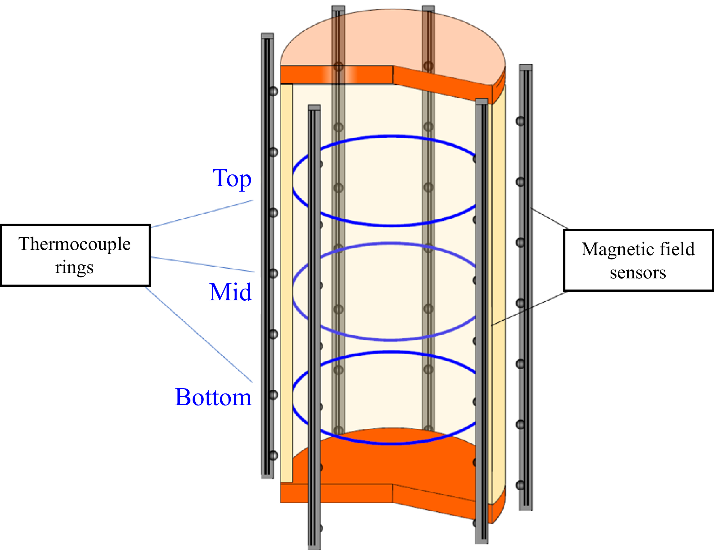
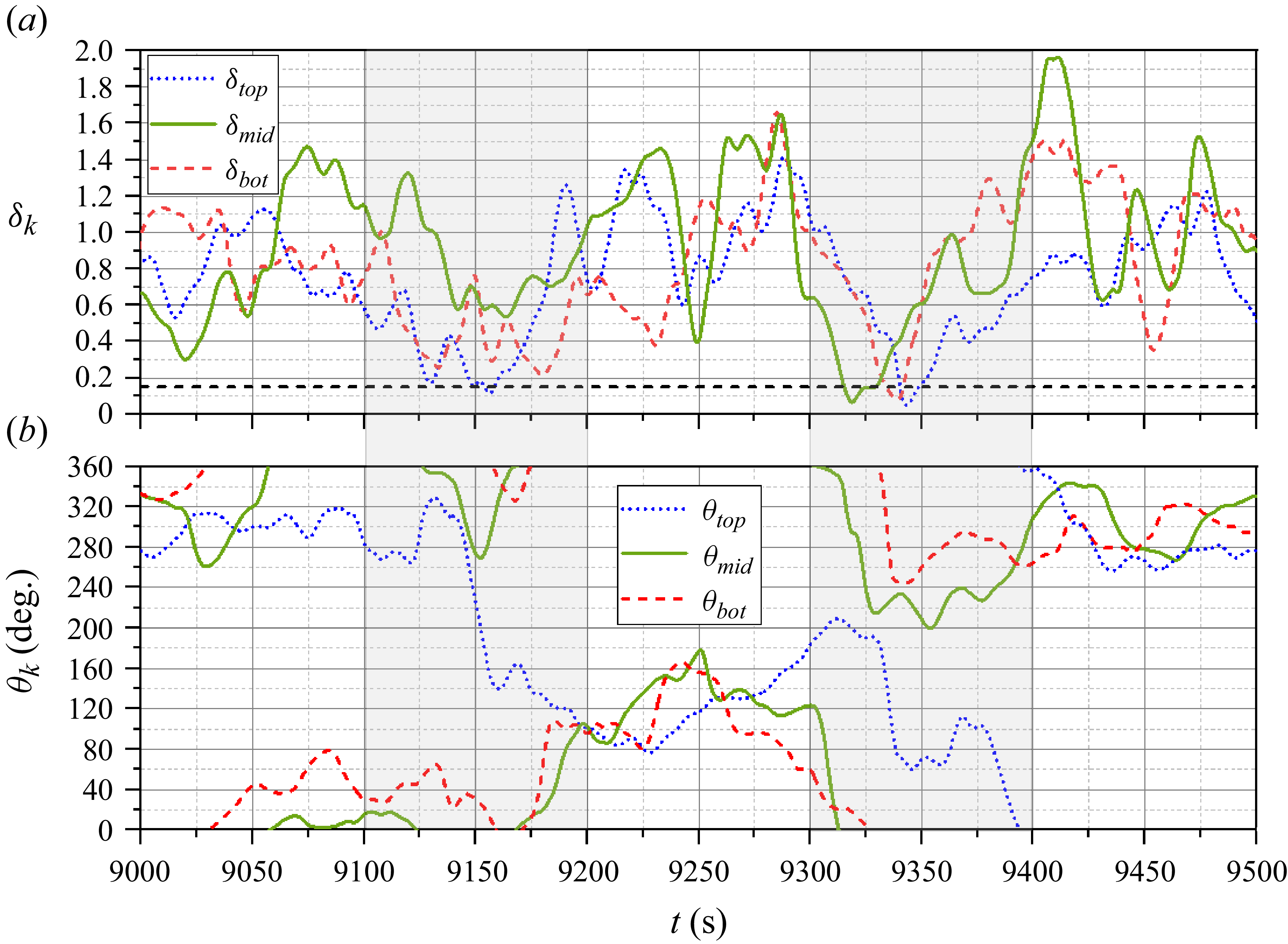
 Ra=6.02×10⁸
 δk
 θk
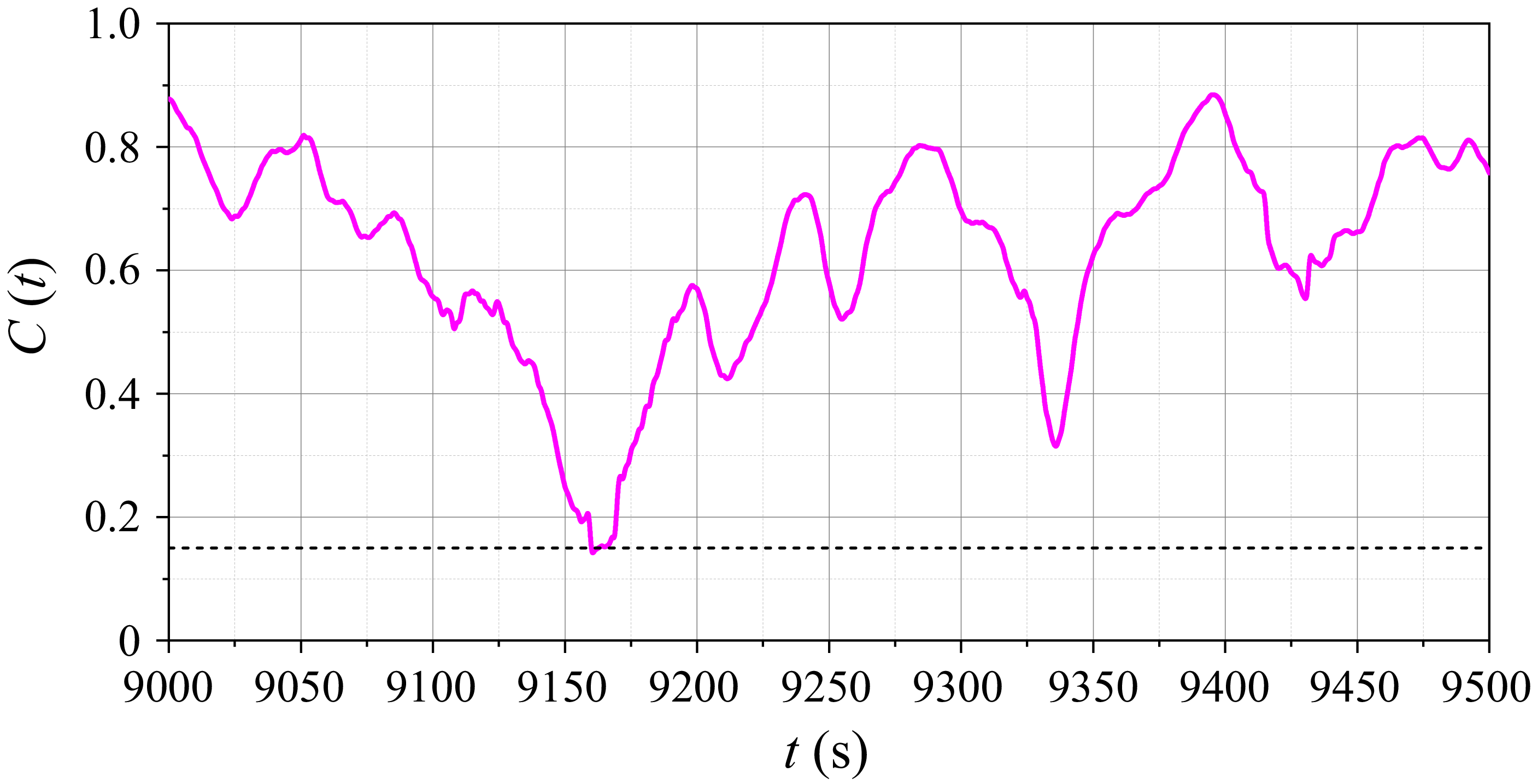
 C(t)=ESRS+DRS/⟨ESRS+DRS⟩
 Ra=6.02×10⁸
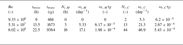
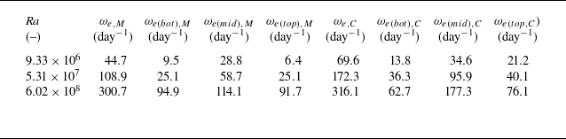

 Pr
 z/H
 z/H
 z/H
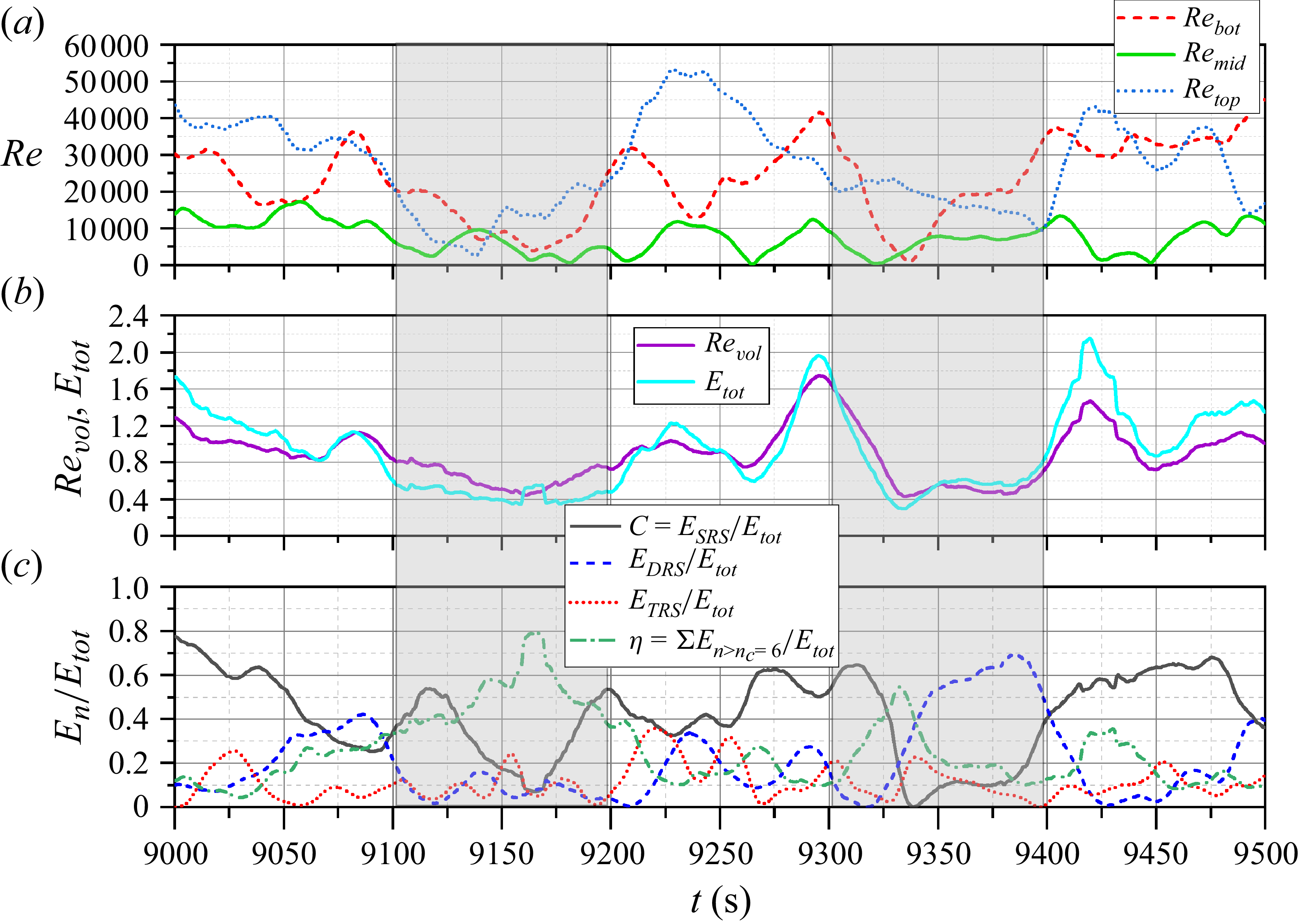
 Ra=6.02×10⁸
 τff=8.65s
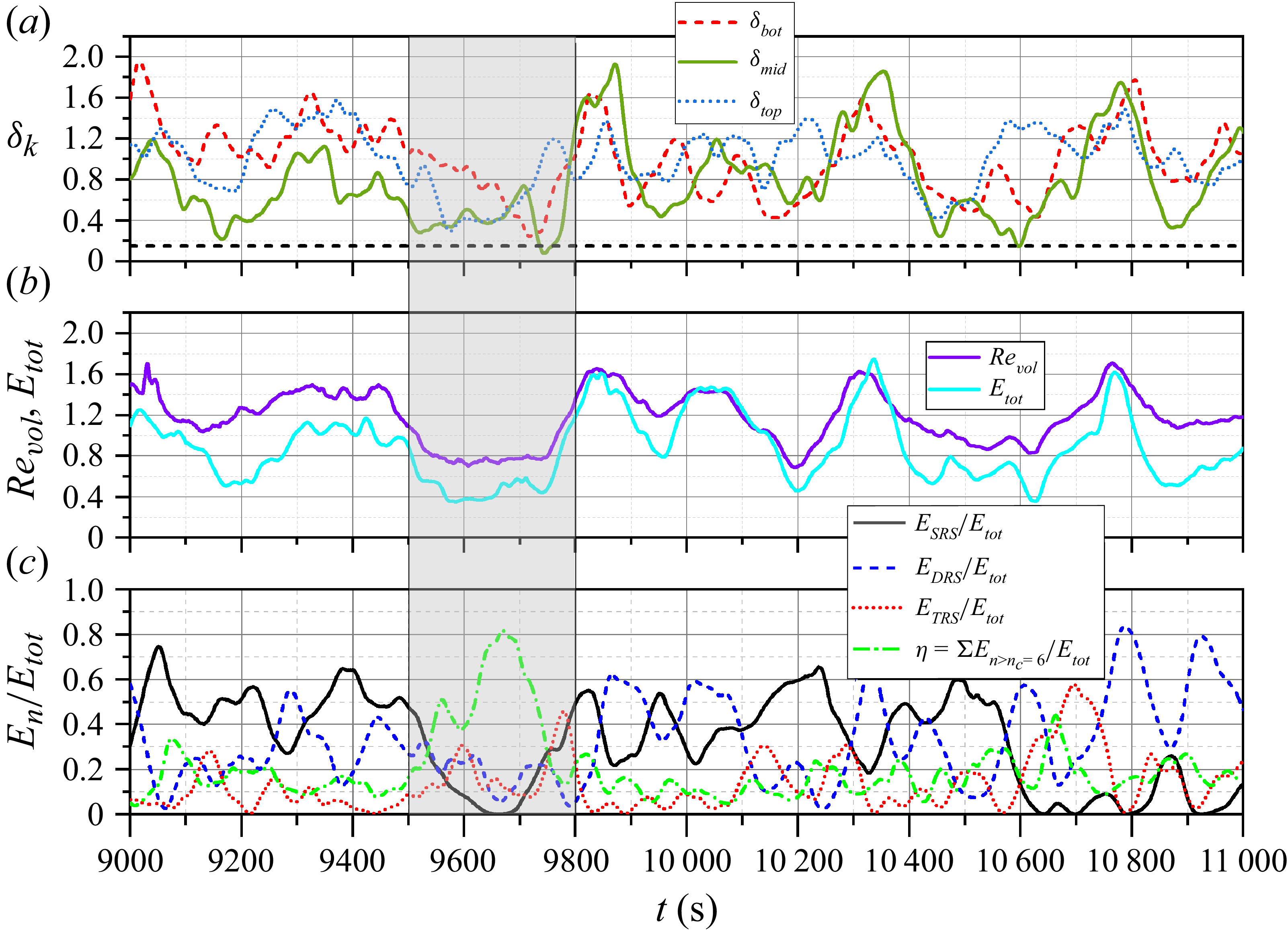
 Ra=5.31×10⁷
 τff=29.04s
 δk

 Ra=6.02×10⁸
 z=3/4H
 z=H/2
 z=1/4H

 Ra=6.02×10⁸
 t≈9160…9180s
 t≈9320…9340s

 Ra=6.02×10⁸
 t=9065s
 t=9100s
 t=9120s
 t=9140s
 t=9150s
 t=9170s
 t=9180s
 t=9190s
 t=9210s
 t=9230s

 Ra=6.02×10⁸
 t=9300s
 t=9320s
 t=9330s
 t=9340s
 t=9350s
 t=9360s
 t=9380s
 t=9400s
 t=9420s
 t=9440s

 Ra=5.31×10⁷
 t=9400s
 t=9480s
 t=9530s
 t=9550s
 t=9580s
 t=9620s
 t=9650s
 t=9690s
 t=9740s
 t=9800s

 Ra=6.02×10⁸
 δk
 t=16100s
 t=16150s
 t=16170s
 t=16280s

 Ra=5.31×10⁷
 ±0.1

 Ra=6.02×10⁸
 ±0.1



