1 Introduction
The Faraday (Reference Faraday1831) instability, in which the interface between two superposed fluid layers subjected to periodic vertical vibration of sufficient amplitude forms sustained standing wave patterns, has been instrumental in the study of pattern formation, leading to the discovery and analysis of hydrodynamic quasipatterns (Edwards & Fauve Reference Edwards and Fauve1994; Rucklidge & Skeldon Reference Rucklidge and Skeldon2015), superlattices (Kudrolli, Pier & Gollub Reference Kudrolli, Pier and Gollub1998; Silber & Proctor Reference Silber and Proctor1998; Arbell & Fineberg Reference Arbell and Fineberg2002), supersquares (Douady Reference Douady1990; Kahouadji et al. Reference Kahouadji, Périnet, Tuckerman, Shin, Chergui and Juric2015) and other exotic patterns (Rajchenbach, Leroux & Clamond Reference Rajchenbach, Leroux and Clamond2011; Périnet, Juric & Tuckerman Reference Périnet, Juric and Tuckerman2012).
Here, we consider a spherical analogue to the Faraday instability, a fluid drop subjected to a time-periodic radial body force. The study of such problems therefore relies particularly on numerical simulation.
Numerical studies of axisymmetric oscillating viscous drops have been carried out by Lundgren & Mansour (Reference Lundgren and Mansour1988) via a boundary-integral method, by Patzek et al. (Reference Patzek, Benner, Basaran and Scriven1991) and Meradji et al. (Reference Meradji, Lyubimova, Lyubimov and Roux2001) via a Galerkin/finite-element method, and by Basaran (Reference Basaran1992) via a marker-in-cell initial-value problem. Tsamopoulos & Brown (Reference Tsamopoulos and Brown1983) used a Poincaré–Lindstedt expansion method to calculate the shapes of axisymmetric inviscid drops subjected to moderate amplitude oscillations for the three lowest capillary modes (see (1.1)). They were unable to confirm mathematically the existence of an asymptotic finite-amplitude motion; this can be verified only by means of numerical calculations. Indeed, the problem of axisymmetric ellipsoidal drop oscillation and decay has now come to be seen as a routine validation test case for numerical codes and interface methods for multiphase flows. However, the full nonlinear problem is non-axisymmetric and requires three-dimensional numerical simulation with interface algorithms that ensure volume conservation and precise calculation of capillary forces as well as the ability to integrate highly spatially resolved systems over long physical times.
Recent advances have led to powerful general purpose codes such as Gerris (Popinet Reference Popinet1993) and BLUE (Shin, Chergui & Juric Reference Shin, Chergui and Juric2017). It is with the multiphase code BLUE, which is based on recently developed hybrid front-tracking/level-set interface methods implemented on parallel computer architectures, that we conduct the current study. We have previously used this code to study large-scale square patterns of Faraday waves (Kahouadji et al. Reference Kahouadji, Périnet, Tuckerman, Shin, Chergui and Juric2015). Here, we use BLUE to carry out the first numerical investigation of the Faraday problem on a sphere.
One of the most appealing aspects of the Faraday instability is that the pattern length scale is not set by the geometry, but by the imposed forcing frequency. (It is this feature which has allowed the generation of quasipatterns and superlattices, since multiple length scales can be excited simultaneously over the entire domain by superposing different frequencies.) This means that for a drop with a fixed radius
 $R$
, patterns can be created with any wavenumber
 $\ell$
, where the interface is described via its spherical harmonic decomposition
 $$\begin{eqnarray}\unicode[STIX]{x1D701}(t,\unicode[STIX]{x1D703},\unicode[STIX]{x1D719})=\mathop{\sum }_{\ell =0}^{\infty }\mathop{\sum }_{m=-\ell }^{m=\ell }\unicode[STIX]{x1D701}_{\ell }^{m}(t)Y_{\ell }^{m}(\unicode[STIX]{x1D703},\unicode[STIX]{x1D719}).\end{eqnarray}$$
For fixed
 $R$
, the length scale associated with
 $\ell$
is
 $R/\ell$
. More importantly,
 $\ell$
is associated with a set of allowed patterns; each value of
 $\ell$
leads to a qualitatively different situation. We will explore the motion and shape of an oscillating drop for values of
 $\ell$
up to 6.
2 Methods
2.1 Pattern formation on a sphere
Our previous paper (Ebo-Adou & Tuckerman Reference Ebo-Adou and Tuckerman2016) concerns the linear stability, via Floquet analysis, of the spherical Faraday problem. As is the case for all spherically symmetric problems, the equation governing the linear stability does not depend on the order
 $m$
of the spherical harmonic. Therefore, a bifurcation from the spherically symmetric state involves
 $2\ell +1$
linearly independent solutions (
 $Y_{\ell }^{m}$
with
 $-\ell \leqslant m\leqslant \ell$
) with the same growth rate. The combination of these modes, i.e. the pattern, that can result from such a bifurcation is determined by the nonlinear terms. A pattern with a given
 $\ell$
cannot be associated with a unique combination of modes
 $m$
, since rotation of a spherical harmonic changes
 $m$
(but not
 $\ell$
).
Symmetry groups provide a classification of patterns which does not depend on orientation. A number of researchers (Busse Reference Busse1975; Busse & Riahi Reference Busse and Riahi1982; Ihrig & Golubitsky Reference Ihrig and Golubitsky1984; Riahi Reference Riahi1984; Golubitsky, Stewart & Schaeffer Reference Golubitsky, Stewart and Schaeffer1988; Chossat, Lauterbach & Melbourne Reference Chossat, Lauterbach and Melbourne1991; Matthews Reference Matthews2003) have studied the patterns which are allowed and those which are preferred for various values of
 $\ell$
. Patterns that appear at bifurcations can be associated with a subgroup of the group
 $O(3)$
of symmetries of the sphere. The subgroups of interest are
 $O(2)$
,
 $D_{k}$
, and the exceptional subgroups
 $T$
,
 $O$
and
 $I$
. Here
 $O(2)$
consists of the symmetries of a circle and patterns which are axisymmetric (for some orientations) are in this category;
 $D_{k}$
describes the symmetries of a
 $k$
-gon, and thus patterns which are invariant under reflection and rotation by
 $2\unicode[STIX]{x03C0}/k$
(about a fixed axis). The three exceptional subgroups are associated with the five Platonic solids:
 $T$
(tetrahedron),
 $O$
(octahedron or cube) and
 $I$
(icosahedron or dodecahedron).
The Platonic solids are regular polyhedra. Although a drop does not have angular vertices and flat faces, a polyhedron with the same symmetry properties can be constructed from a drop in a
 $T$
,
 $O$
, or
 $I$
configuration by assigning a local maximum on the surface to a vertex and a local minimum to a face. The dual of a polyhedron is obtained by inverting its vertices with its faces, an operation which preserves symmetry. Similarly, the dual of a drop can be formed by inverting maxima and minima. An oscillating drop provides an ideal opportunity to observe duality: since a location which is the site of a maximum contains a minimum after half of an oscillation period, the interface alternates between a pattern and its dual. For the Platonic solids, the dual of an octahedron is a cube, that of an icosahedron is a dodecahedron, and the dual of a tetrahedron is another tetrahedron.
The patterns are highly dependent on the value of
 $\ell$
considered. Axisymmetric (sometimes called zonal) solutions are never stable if
 $\ell \geqslant 2$
(Chossat et al.
Reference Chossat, Lauterbach and Melbourne1991). For odd
 $\ell$
, solutions exist which are stable at onset. In contrast, for even
 $\ell$
, all solutions are unstable near the bifurcation point. In this case, the preferred solution can be considered to be that with the smallest number of unstable eigenvalues (Matthews Reference Matthews2003) or which extremizes a functional (Busse Reference Busse1975). Unstable solution branches produced at a transcritical bifurcation can be stabilized (for example, at a saddle-node bifurcation some distance from the threshold).
The theory of pattern selection with
 $O(3)$
symmetry differs from the framework of our simulations in some important ways. First, the theory applies to steady bifurcations rather than oscillatory solutions resulting from time-periodic forcing. The archetypical application is Rayleigh–Bénard convection in a sphere (Busse Reference Busse1975; Busse & Riahi Reference Busse and Riahi1982; Riahi Reference Riahi1984) and the steady symmetry-breaking bifurcations it undergoes. However, many of the conclusions can be generalized to the time-periodic context, by considering the discrete-time dynamical system derived by sampling the continuous-time system at a single phase of the forcing period.
Second, the theory applies close to the threshold. Our simulations are carried out far from threshold, so that instabilities can grow on a reasonable time scale and stabilize at an amplitude that can be clearly seen. Our patterns contain modes generated by nonlinear interactions and their existence or stability may result from secondary bifurcations.
Despite these differences, we will see that there is much common ground between the patterns we observe and those predicted by theory.
2.2 Problem formulation, governing equations and numerical scheme
The governing equations for an incompressible two-phase flow can be expressed by a single field formulation:
 $$\begin{eqnarray}\unicode[STIX]{x1D70C}\left(\frac{\unicode[STIX]{x2202}\boldsymbol{u}}{\unicode[STIX]{x2202}t}+\boldsymbol{u}\boldsymbol{\cdot }\unicode[STIX]{x1D735}\boldsymbol{u}\right)=-\unicode[STIX]{x1D735}P+\unicode[STIX]{x1D70C}\boldsymbol{G}+\unicode[STIX]{x1D735}\boldsymbol{\cdot }\unicode[STIX]{x1D707}(\unicode[STIX]{x1D735}\boldsymbol{u}+\unicode[STIX]{x1D735}\boldsymbol{u}^{\text{T}})+\boldsymbol{F},\quad \unicode[STIX]{x1D735}\boldsymbol{\cdot }\boldsymbol{u}=0,\end{eqnarray}$$
where
 $\boldsymbol{u}$
is the velocity,
 $P$
is the pressure,
 $\unicode[STIX]{x1D70C}$
is the density,
 $\unicode[STIX]{x1D707}$
is the dynamic viscosity and
 $\boldsymbol{F}$
is the local surface tension force at the interface. Here,
 $\boldsymbol{G}$
is an imposed time-dependent radial acceleration:
 $$\begin{eqnarray}\boldsymbol{G}=-(g+a\cos (\unicode[STIX]{x1D714}t))\frac{r}{R}\boldsymbol{e}_{r},\end{eqnarray}$$
where
 $g$
is a constant acceleration, referred to for simplicity as gravitational, which is set to zero when we carry out capillary simulations. Here
 $R$
is the radius of the drop,
 $\boldsymbol{e}_{r}$
is the radial unit vector, and
 $a$
and
 $\unicode[STIX]{x1D714}$
are the amplitude and frequency of the oscillatory forcing.
Material properties such as density or viscosity are defined in the entire domain:
 $$\begin{eqnarray}\left.\begin{array}{@{}c@{}}\unicode[STIX]{x1D70C}(\boldsymbol{x},t)=\unicode[STIX]{x1D70C}_{1}+(\unicode[STIX]{x1D70C}_{2}-\unicode[STIX]{x1D70C}_{1})I(\boldsymbol{x},t)\\ \unicode[STIX]{x1D707}(\boldsymbol{x},t)=\unicode[STIX]{x1D707}_{1}+(\unicode[STIX]{x1D707}_{2}-\unicode[STIX]{x1D707}_{1})I(\boldsymbol{x},t).\end{array}\right\}\end{eqnarray}$$
The indicator function
 $I$
in (2.3) is the Heaviside function, whose value is zero in one phase and unity in the other phase. In our discrete numerical implementation
 $I$
is approximated by
 $I_{num}$
, which represents a smooth transition across three to four grid cells, as pioneered in the immersed boundary method of Peskin (Reference Peskin1977). In our method,
 $I_{num}$
is generated using a vector distance function computed directly from the tracked interface (Shin & Juric Reference Shin and Juric2009).
The fluid variables
 $\boldsymbol{u}$
and
 $P$
are calculated by a projection method (Chorin Reference Chorin1968). The temporal scheme is first order, with implicit time integration used for the viscous terms. For spatial discretization we use the staggered-mesh marker-in-cell (MAC) method (Harlow & Welch Reference Harlow and Welch1965) on a uniform finite-difference grid with second-order essentially non-oscillatory (ENO) advection (Shu & Osher Reference Shu and Osher1989). The pressure and distance function are located at cell centres while the
 $x$
,
 $y$
and
 $z$
components of velocity are located at the faces. All spatial derivatives are approximated by standard second-order centred differences. The treatment of the free surface uses a hybrid Front-Tracking/Level-Set technique which defines the interface both by the Level-Set distance function field on the Eulerian grid as well as by triangles on the Lagrangian interface mesh.
The surface tension
 $\boldsymbol{F}$
is implemented by the hybrid/compact formulation (Shin Reference Shin2007)
 $$\begin{eqnarray}\boldsymbol{F}=\unicode[STIX]{x1D70E}\unicode[STIX]{x1D705}_{H}\unicode[STIX]{x1D735}I,\quad \unicode[STIX]{x1D705}_{H}=\frac{\boldsymbol{F}_{L}\boldsymbol{\cdot }\boldsymbol{N}}{\boldsymbol{N}\boldsymbol{\cdot }\boldsymbol{N}},\end{eqnarray}$$
where
 $\unicode[STIX]{x1D70E}$
is the surface tension coefficient and
 $\unicode[STIX]{x1D705}_{H}$
is twice the mean interface curvature field calculated on the Eulerian grid, with
 $$\begin{eqnarray}\boldsymbol{F}_{_{L}}=\int _{\unicode[STIX]{x1D6E4}(t)}\unicode[STIX]{x1D705}_{f}\boldsymbol{n}_{f}\unicode[STIX]{x1D6FF}_{f}(\boldsymbol{x}-\boldsymbol{x}_{f})\,\text{d}a,\quad \boldsymbol{N}=\int _{\unicode[STIX]{x1D6E4}(t)}\boldsymbol{n}_{f}\unicode[STIX]{x1D6FF}_{f}(\boldsymbol{x}-\boldsymbol{x}_{f})\,\text{d}a.\end{eqnarray}$$
Here,
 $\boldsymbol{x}_{f}$
is a parameterization of the time-dependent interface,
 $\unicode[STIX]{x1D6E4}(t)$
, and
 $\unicode[STIX]{x1D6FF}_{f}(\boldsymbol{x}-\boldsymbol{x}_{f})$
is a Dirac distribution that is non-zero only where
 $\boldsymbol{x}=\boldsymbol{x}_{f}$
;
 $\boldsymbol{n}_{f}$
stands for the unit normal vector to the interface and
 $\text{d}a$
is the area of an interface element;
 $\unicode[STIX]{x1D705}_{f}$
is twice the mean interface curvature obtained on the Lagrangian interface. The geometric information, unit normal,
 $\boldsymbol{n}_{f}$
, and interface element length,
 $\text{d}a$
, in
 $\boldsymbol{N}$
are computed directly from the Lagrangian interface and then distributed onto the Eulerian grid using the discrete delta function and the immersed boundary method of Peskin (Reference Peskin1977). A detailed description of the procedure for calculating
 $\boldsymbol{F}$
,
 $\boldsymbol{N}$
and
 $I_{num}$
can be found in Shin & Juric (Reference Shin and Juric2007, Reference Shin and Juric2009), where in particular we demonstrate that this method of calculating the surface tension force reduces any parasitic currents in the standard static drop test case to a level of
 $O(10^{-7})$
for fluids with properties similar to those we use here.
The Lagrangian interface is advected by integrating
 $\text{d}\boldsymbol{x}_{f}/\text{d}t=\boldsymbol{V}$
with a second-order Runge–Kutta method, where the interface velocity,
 $\boldsymbol{V}$
, is interpolated from the Eulerian velocity.
The parallelization of the code is based on algebraic domain decomposition, where the velocity field is solved by a parallel generalized minimum residual (GMRES) method for the implicit viscous terms and the pressure by a parallel multigrid method motivated by the algorithm of Kwak & Lee (Reference Kwak and Lee2004). Communication across process threads is handled by message passing interface (MPI) procedures.
The code contains a module for the definition of immersed solid objects and their interaction with the flow, which we have used to simulate Faraday waves in a spherical container. In order to simulate a fluid within a solid sphere we take the simple approach of defining all grid cells whose centres lie within the solid region as solid. Then Dirichlet (no-slip) boundary conditions for the velocity and Neumann conditions for the pressure are applied to those cell faces as in the projection method. On a Cartesian grid this necessarily creates a stair-stepped solid/fluid boundary; however, it is found that the method works well in practice since the discrete momentum flux is conserved and is simpler than and equivalent to other approaches which impose a near-wall force to ensure a no-slip condition at the solid (Tryggvason, Scardovelli & Zaleski Reference Tryggvason, Scardovelli and Zaleski2011). See Shin et al. (Reference Shin, Chergui and Juric2017) for further details.
2.3 Physical parameters of the fluids
Our numerical code can treat inner and outer spherical domains of any size containing fluids of any density
 $\unicode[STIX]{x1D70C}$
, viscosity
 $\unicode[STIX]{x1D708}$
, and surface tension
 $\unicode[STIX]{x1D70E}$
, leading potentially to a large number of non-dimensional parameters, in addition to those describing the forcing amplitude
 $a$
and frequency
 $\unicode[STIX]{x1D714}$
. We have chosen to limit the parameter space as follows.
The density and viscosity ratios that we have chosen are typical of oil droplets in air. The inner and outer densities are
 $\unicode[STIX]{x1D70C}_{d}=940~\text{kg}~\text{m}^{-3}$
and
 $\unicode[STIX]{x1D70C}_{out}=1.205~\text{kg}~\text{m}^{-3}$
, leading to the density ratio
 $\unicode[STIX]{x1D70C}_{d}/\unicode[STIX]{x1D70C}_{out}=780$
, while the inner and outer kinematic viscosities are
 $\unicode[STIX]{x1D708}_{d}=10^{-5}~\text{m}^{2}~\text{s}^{-1}$
and
 $\unicode[STIX]{x1D708}_{out}=1.5\times 10^{-5}~\text{m}^{2}~\text{s}^{-1}$
, leading to the viscosity ratio
 $\unicode[STIX]{x1D708}_{d}/\unicode[STIX]{x1D708}_{out}=0.66$
. The viscosity of both fluids is sufficiently low that the stability diagram approaches that of the Mathieu equation. (One of the conclusions of Ebo-Adou & Tuckerman (Reference Ebo-Adou and Tuckerman2016) is that the Mathieu equation describes the inviscid Faraday instability even in a spherical geometry.) More specifically,
 $\unicode[STIX]{x1D708}_{d}/(R^{2}\unicode[STIX]{x1D714})$
is between
 $3\times 10^{-4}$
and
 $7\times 10^{-3}$
for the capillary cases and between
 $6\times 10^{-4}$
and
 $9\times 10^{-4}$
for the gravitational cases. Usually, Faraday waves are subharmonic, i.e. their period is twice the forcing period
 $T$
. However, in this low-viscosity regime, we can easily excite harmonic waves as well (Kumar Reference Kumar1996), whose period is the same as the forcing period.
For the capillary cases, we set the surface tension to be
 $\unicode[STIX]{x1D70E}=0.02~\text{kg}~\text{s}^{-2}$
, the constant radial acceleration to be
 $g=0$
, and the drop radius to be
 $R=0.06$
m, while for the gravitational cases, we set the constant radial acceleration to be
 $g=-1~\text{m}~\text{s}^{-2}$
, the surface tension to be
 $\unicode[STIX]{x1D70E}=0$
, and the drop radius to be
 $R=0.05$
m. We will use these parameters to non-dimensionalize the forcing frequencies and amplitudes as in (2.15), and we list these in § 2.7 and table 3.
2.4 Numerical parameters
For the capillary cases, the domain is a sphere whose radius is
 $2R$
(see § 2.2 and figures 8 and 9). The Eulerian mesh is uniform and Cartesian, with a resolution of
 $N_{x}^{3}$
, which is generally
 $128^{3}$
. The Lagrangian triangular grid used to represent the interface is constructed in such a way that the sides of the triangles remain close to the length of the diagonals of the cubic Eulerian mesh. The grid spacing
 $\unicode[STIX]{x0394}x=4R/N_{x}$
for the capillary cases should be compared to the circumference
 $2\unicode[STIX]{x03C0}R$
of the drop and to the approximate wavelengths
 $2\unicode[STIX]{x03C0}R/\ell$
. The radius and circumference are spanned by
 $R/\unicode[STIX]{x0394}x=N_{x}/4$
and
 $2\unicode[STIX]{x03C0}R/\unicode[STIX]{x0394}x=N_{x}\unicode[STIX]{x03C0}/2$
, which are 32 and 201, respectively, for the
 $128^{3}$
grid. The number of gridpoints per wavelength
 $N_{x}\unicode[STIX]{x03C0}/(2\ell )$
goes from 201 for
 $\ell =1$
to 33 points for
 $\ell =6$
for this grid. The interface is represented by approximately
 $4\unicode[STIX]{x03C0}R^{2}/(\unicode[STIX]{x0394}x)^{2}=N_{x}^{2}\unicode[STIX]{x03C0}/4$
points, i.e. 12 868 points for
 $N_{x}=128$
. For the gravitational cases, the radius of the bounding sphere is
 $2.4R$
, leading to slightly different but similar numbers for the resolution (for example,
 $R/\unicode[STIX]{x0394}x=26.7$
rather than 32). We have also carried out simulations with grids of
 $256^{3}$
(to confirm our results) and of
 $64^{3}$
(for visualization of our patterns). Parallelization is achieved through domain decomposition, in which each subdomain is assigned to its own process thread. Here, we use
 $512$
subdomains or processes, each with
 $16^{3}$
or
 $32^{3}$
gridpoints for the global resolutions of
 $128^{3}$
and
 $256^{3}$
, respectively.
The time step
 $\unicode[STIX]{x0394}t$
is chosen at each iteration in order to satisfy a criterion based on
 $$\begin{eqnarray}\{\unicode[STIX]{x0394}t_{CFL},\unicode[STIX]{x0394}t_{int},\unicode[STIX]{x0394}t_{vis},\unicode[STIX]{x0394}t_{cap}\},\end{eqnarray}$$
which ensures stability of the calculations. These bounds are defined by:
 $$\begin{eqnarray}\left.\begin{array}{@{}c@{}}\displaystyle \unicode[STIX]{x0394}t_{CFL}\equiv \min _{j}\left(\min _{domain}\left(\frac{\unicode[STIX]{x0394}x_{j}}{u_{j}}\right)\right),\quad \unicode[STIX]{x0394}t_{int}\equiv \min _{j}\left(\min _{\unicode[STIX]{x1D6E4}(t)}\left(\frac{\unicode[STIX]{x0394}x_{j}}{\Vert \boldsymbol{V}\Vert }\right)\right)\\ \displaystyle \unicode[STIX]{x0394}t_{vis}\equiv \min \left(\frac{\unicode[STIX]{x1D70C}_{2}}{\unicode[STIX]{x1D707}_{2}},\frac{\unicode[STIX]{x1D70C}_{1}}{\unicode[STIX]{x1D707}_{1}}\right)\frac{\unicode[STIX]{x0394}x_{min}^{2}}{6},\quad \unicode[STIX]{x0394}t_{cap}\equiv \frac{1}{2}\left(\frac{(\unicode[STIX]{x1D70C}_{1}+\unicode[STIX]{x1D70C}_{2})\unicode[STIX]{x0394}x_{min}^{3}}{\unicode[STIX]{x03C0}\unicode[STIX]{x1D70E}}\right)^{1/2},\end{array}\right\}\end{eqnarray}$$
where
 $\unicode[STIX]{x0394}x_{min}=\min _{j}(\unicode[STIX]{x0394}x_{j})$
. In our simulations, this minimum is realized by
 $\unicode[STIX]{x0394}t_{CFL}\approx \unicode[STIX]{x0394}t_{int}$
for our gravitational waves and by
 $\unicode[STIX]{x0394}t_{cap}\approx \unicode[STIX]{x0394}t_{vis}$
for our capillary waves.
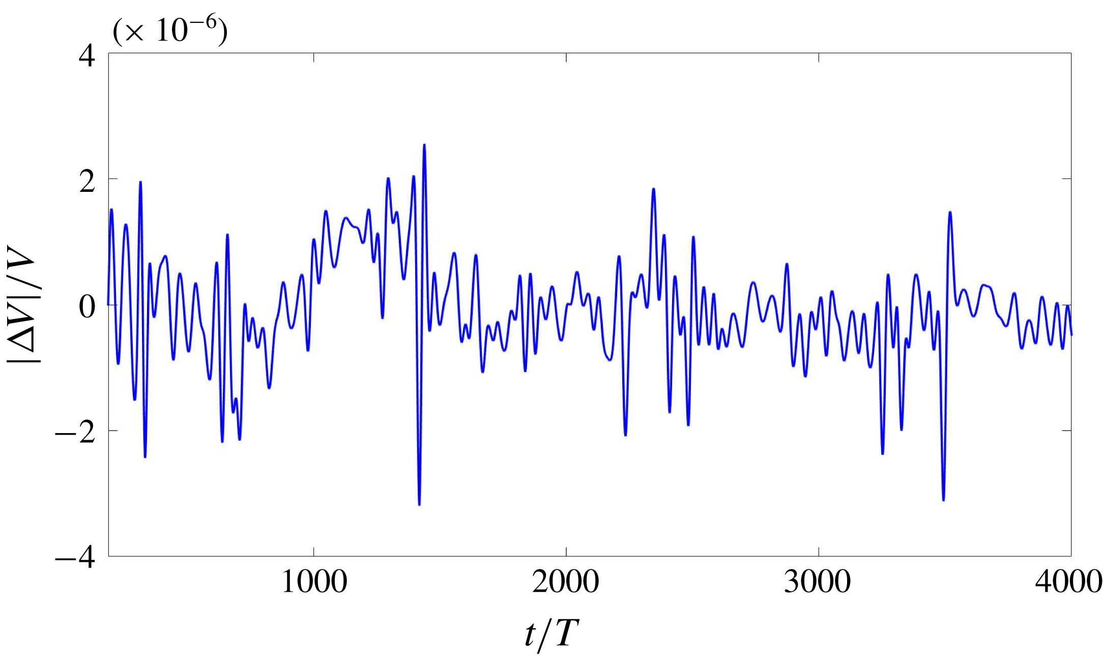
Time evolution of the normalized deviation of
 $\unicode[STIX]{x0394}V(t)/V$
for a simulation with
 $\ell =6$
. The value of
 $|\unicode[STIX]{x0394}V|/V$
remains less than approximately
 $3\times 10^{-6}$
throughout the simulation.

2.5 Spherical harmonic transform
In order to analyse the shape of the drop quantitatively, we will compute and present the time-dependent spectral coefficients, obtained from the decomposition
 $$\begin{eqnarray}\unicode[STIX]{x1D701}(\unicode[STIX]{x1D703},\unicode[STIX]{x1D719},t)=\mathop{\sum }_{\ell =0}^{\infty }\mathop{\sum }_{m=-\ell }^{m=\ell }\unicode[STIX]{x1D701}_{\ell }^{m}(t)Y_{\ell }^{m}(\unicode[STIX]{x1D703},\unicode[STIX]{x1D719}),\end{eqnarray}$$
where
 $\unicode[STIX]{x1D701}$
is the distance from the domain centre. We compute both
 $|\unicode[STIX]{x1D701}_{\ell }^{m}(t)|$
and
 $$\begin{eqnarray}\unicode[STIX]{x1D701}_{\ell }(t)\equiv \left[\mathop{\sum }_{m=0}^{\ell }|\unicode[STIX]{x1D701}_{\ell }^{m}(t)|^{2}\right]^{1/2}.\end{eqnarray}$$
We note that, according to the normalization convention we use,
 $$\begin{eqnarray}\unicode[STIX]{x1D701}_{0}(t)=\unicode[STIX]{x1D701}_{0}^{0}=\int _{0}^{2\unicode[STIX]{x03C0}}\,\text{d}\unicode[STIX]{x1D719}\int _{0}^{\unicode[STIX]{x03C0}}\,\text{d}\unicode[STIX]{x1D703}\sin \unicode[STIX]{x1D703}\unicode[STIX]{x1D701}(\unicode[STIX]{x1D703},\unicode[STIX]{x1D719},t)Y_{0}^{0}(\unicode[STIX]{x1D703},\unicode[STIX]{x1D719})\end{eqnarray}$$
i.e.
 $\unicode[STIX]{x1D701}_{0}(t)$
is
 $\sqrt{4\unicode[STIX]{x03C0}}$
times the spherically averaged distance of the interface from the origin.
We calculate the spherical harmonic transform as follows. The three-dimensional Lagrangian interface consists of triangles composed of points
 $(x_{i},y_{i},z_{i})$
on the fixed Cartesian grid. We transform each of these points to spherical coordinates
 $(\unicode[STIX]{x1D701}_{i},\unicode[STIX]{x1D703}_{i},\unicode[STIX]{x1D719}_{i})$
and interpolate the function
 $\unicode[STIX]{x1D701}(\unicode[STIX]{x1D703}_{i},\unicode[STIX]{x1D719}_{i})=\unicode[STIX]{x1D701}_{i}$
onto a regular spherical grid
 $(\unicode[STIX]{x1D703}_{j},\unicode[STIX]{x1D719}_{k})$
, discretizing the latitudinal interval
 $[0,\unicode[STIX]{x03C0}]$
and longitudinal interval
 $[0,2\unicode[STIX]{x03C0}]$
with
 $N_{\unicode[STIX]{x1D703}}=80$
and
 $N_{\unicode[STIX]{x1D719}}=80$
points. Using the discrete data
 $\unicode[STIX]{x1D701}(\unicode[STIX]{x1D703}_{j},\unicode[STIX]{x1D719}_{k})$
and truncating the series (2.8) at four times the dominant value of
 $\ell$
, we compute the spherical harmonic coefficients
 $\unicode[STIX]{x1D701}_{\ell }^{m}$
by the method of least squares (Politis Reference Politis2013, Reference Politis2016). This procedure is carried out for each sampled temporal snapshot of the interface. We note that the spherical harmonic coefficients are weighted averages of the surface height over the entire drop surface, and hence more accurate than the individual surface height values.
The spectrum in
 $m$
(but not in
 $\ell$
) depends on the orientation. We can rotate a pattern by localizing the coordinates
 $(\unicode[STIX]{x1D703},\unicode[STIX]{x1D719})$
of one of its features, such as a maximum, rotating in longitude
 $\unicode[STIX]{x1D719}$
to place it in the
 $(x,z)$
plane and then rotating in colatitude
 $\unicode[STIX]{x1D703}$
to place this feature at the north pole. This allows us to interpret our spectra by using the explicit representations given by Busse (Reference Busse1975) of various patterns in terms of
 $Y_{\ell }^{m}$
. Conversely, if the shape of the pattern is known or constant, the spectrum in
 $m$
can be used to track changes in its orientation.
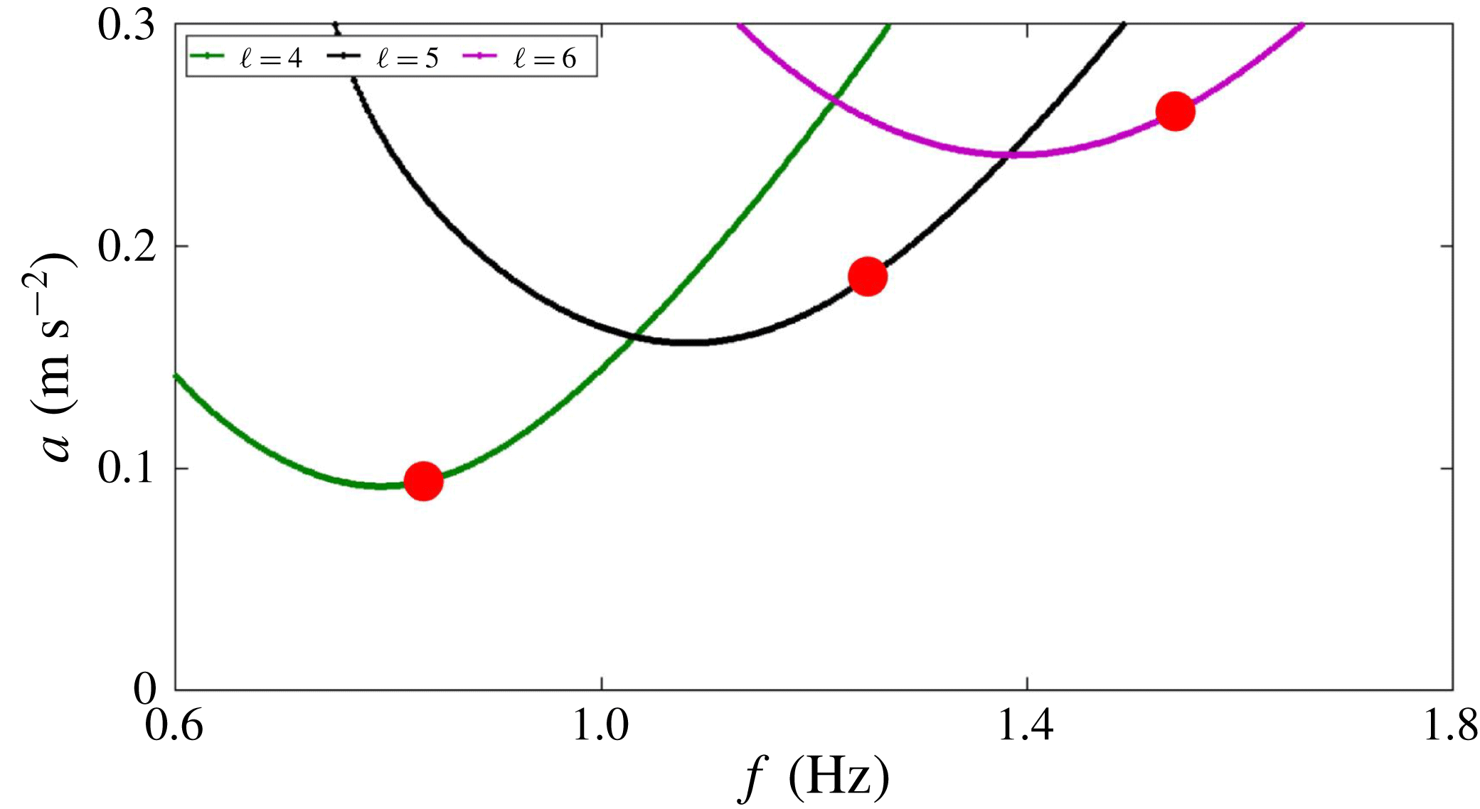
Comparison between the theoretical and computed threshold
 $a_{c}$
Curves show theoretical thresholds calculated from Floquet theory (Ebo-Adou & Tuckerman Reference Ebo-Adou and Tuckerman2016) for
 $\ell =4$
, 5, 6, while circles show results from numerical simulations with resolution
 $256^{3}$
at the indicated frequencies calculated by the method shown in figure 3.

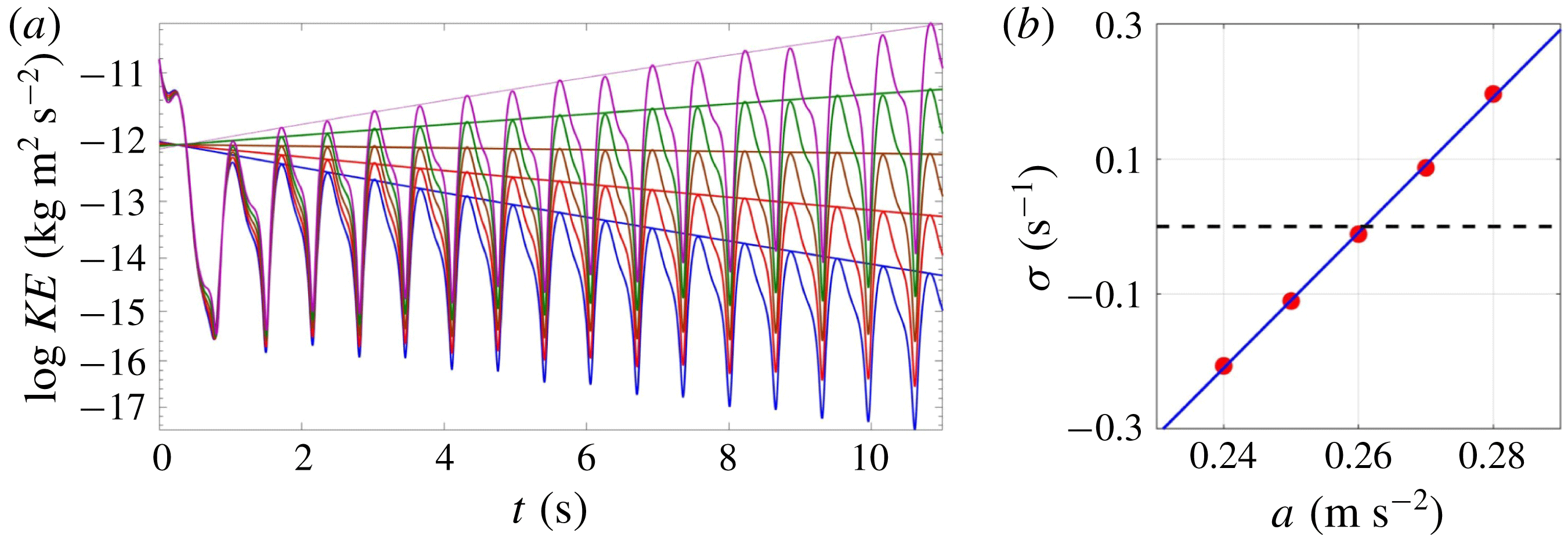
Calculation of thresholds. (a) Time series of interface height oscillate and grow or decay exponentially, depending on the imposed acceleration amplitude, as shown by the linear time dependence of the logarithms of the peaks. (b) The slopes of the logarithms of the time series maxima constitute the growth or decay rates, which are interpolated to determine the acceleration amplitude threshold for
 $\ell =6$
, shown as the rightmost circle in figure 2.

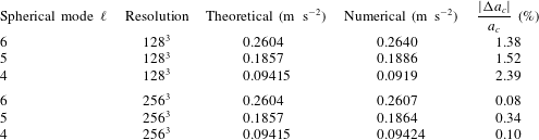
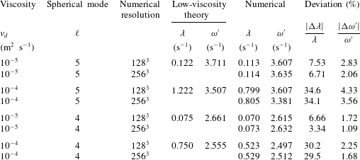
Comparison between theoretical and computed thresholds
 $a_{c}$
for various
 $\ell$
values and numerical resolutions.

2.6 Validation
The front-tracking approach inherently conserves mass to high accuracy compared to other numerical interface methods (Shin & Juric Reference Shin and Juric2009). We confirm mass conservation by showing the fractional deviation of the volume. Figure 1 shows the time evolution of the bounding envelope of
 $\unicode[STIX]{x0394}V/V$
for a simulation with resolution
 $128^{3}$
. The fluid parameters are those of § 2.3 and table 3 for the
 $\ell =6$
case. (See figure 11 for an illustration of the extraction of the bounding envelope.) We see that
 $|\unicode[STIX]{x0394}V(t)|/V$
remains less than approximately
 $3\times 10^{-6}$
throughout the simulation.
In our previous investigation (Ebo-Adou & Tuckerman Reference Ebo-Adou and Tuckerman2016), we extended the method of Kumar & Tuckerman (Reference Kumar and Tuckerman1994) for computing the Faraday threshold via Floquet theory to a spherical geometry. In figure 2 and table 1 we compare these theoretical results with thresholds obtained by interpolating growth rates from numerical simulations, as shown in figure 3. The parameters are as previously stated for capillary waves in § 2.3, except that we increase the viscosity to
 $\unicode[STIX]{x1D708}_{d}=10^{-4}~\text{m}^{2}~\text{s}^{-1}$
. For
 $\ell =6$
, the error in the threshold is approximately 1 % for a resolution of
 $128^{3}$
and only approximately 0.1 % for a resolution of
 $256^{3}$
.
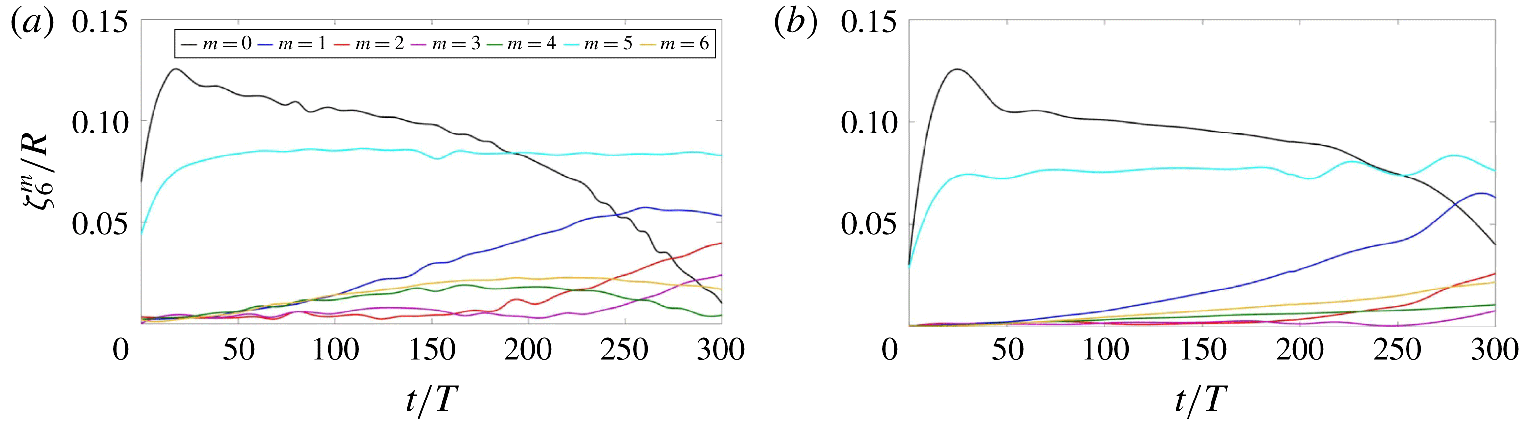
Comparison of evolution of spherical harmonic spectra
 $Y_{6}^{m}$
for resolutions (a)
 $128^{3}$
and (b)
 $256^{3}$
.

Figure 4 compares the time evolution of the envelope of the spherical harmonic coefficients
 $|\unicode[STIX]{x1D701}_{\ell }^{m}|$
for capillary wave simulations using resolutions
 $128^{3}$
and
 $256^{3}$
. The fluid parameters are again those of § 2.3 and table 3 for the
 $\ell =6$
case. Starting from an icosahedral initial condition, the solution evolves similarly for the two spatial resolutions. The main difference is that near-zero modes grow more slowly for the higher resolution, which can be understood as a manifestation of the lower level of noise introduced in the simulation.
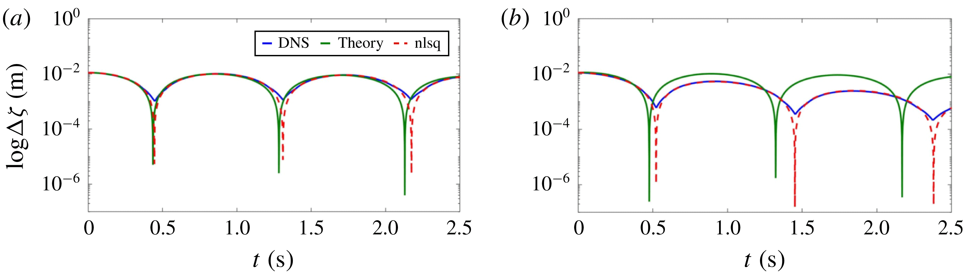
Free decay of a shape-deformed drop to the spherical shape. The evolution of
 $\unicode[STIX]{x0394}\unicode[STIX]{x1D701}\equiv \unicode[STIX]{x1D701}_{max}-\unicode[STIX]{x1D701}_{min}$
with time is shown for
 $\ell =5$
for a resolution of
 $256^{3}$
. The blue curve corresponds to the output from numerical simulations which is fitted by a nonlinear least-square method (dashed red). The green curve corresponds to the small-viscosity-limit prediction for viscosity (a)
 $\unicode[STIX]{x1D708}_{d}=10^{-5}~\text{m}^{2}~\text{s}^{-1}$
and (b)
 $\unicode[STIX]{x1D708}_{d}=10^{-4}~\text{m}^{2}~\text{s}^{-1}$
.


We also validated our numerical code by testing the free decay of a perturbed sphere in the unforced case (i.e.
 $a=0$
, no imposed oscillatory forcing) under the influence of surface tension. In the absence of viscosity, Rayleigh (Reference Rayleigh1879) showed that a drop initialized with a perturbation of spherical wavenumber
 $\ell$
oscillates with frequency
 $\unicode[STIX]{x1D714}$
, where
 $$\begin{eqnarray}\unicode[STIX]{x1D714}^{2}=\frac{\unicode[STIX]{x1D70E}}{\unicode[STIX]{x1D70C}}\frac{\ell (\ell -1)(\ell +2)}{R^{3}}.\end{eqnarray}$$
For small kinematic viscosity
 $\unicode[STIX]{x1D708}_{d}$
, Lamb (Reference Lamb1932) showed that the oscillation amplitude decays to the spherical rest state according to
 $$\begin{eqnarray}\unicode[STIX]{x1D701}_{\ell }(t)\propto \text{e}^{-\unicode[STIX]{x1D706}t}|\text{cos}(\unicode[STIX]{x1D714}^{\prime }t)|,\end{eqnarray}$$
where the decay rate and the oscillation frequency are given by
 $$\begin{eqnarray}\unicode[STIX]{x1D706}=\frac{\unicode[STIX]{x1D708}_{d}(\ell -1)(2\ell +1)}{R^{2}},\quad \unicode[STIX]{x1D714}^{\prime }=(\unicode[STIX]{x1D714}^{2}-\unicode[STIX]{x1D706}^{2})^{1/2}.\end{eqnarray}$$
Figure 5 shows the evolution of
 $\unicode[STIX]{x0394}\unicode[STIX]{x1D701}\equiv \unicode[STIX]{x1D701}_{max}-\unicode[STIX]{x1D701}_{min}$
obtained via numerical simulations with a resolution of
 $256^{3}$
of capillary waves with the fluid parameters of § 2.3 initialized with axisymmetric perturbations
 $Y_{5}^{0}$
for two different viscosities, along with curves obtained from the low-viscosity theory of (2.12)–(2.13). Table 2 gives the values of the decay rates and nonlinear frequencies from figure 5, along with additional cases in which the spherical mode and the spatial resolution have been varied. As could be expected, the deviation is lowest when the resolution is higher (
 $256^{3}$
) so that the simulation is more accurate, and when the viscosity is lower (
 $\unicode[STIX]{x1D708}_{d}=10^{-5}~\text{m}~\text{s}^{-2}$
) so that the low-viscosity theory is more applicable. This best-case deviation is approximately 7 % for
 $\unicode[STIX]{x1D706}$
and 2 % for
 $\unicode[STIX]{x1D714}^{\prime }$
for
 $\ell =5$
, and only approximately 3 % for
 $\unicode[STIX]{x1D706}$
and 1 % for
 $\unicode[STIX]{x1D714}^{\prime }$
for
 $\ell =4$
.
2.7 Survey of cases studied
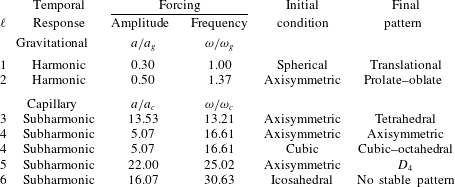
Table 3 lists the simulations which we will describe in this paper. As an initial condition, we perturb the spherical interface by one of the following combinations of spherical harmonics:
 $$\begin{eqnarray}\displaystyle & \displaystyle \text{Axisymmetric all }\ell \quad \unicode[STIX]{x1D701}-R\propto Y_{\ell }^{0} & \displaystyle\end{eqnarray}$$
 $$\begin{eqnarray}\displaystyle & \displaystyle \text{Tetrahedral }\ell =3\quad \unicode[STIX]{x1D701}-R\propto Y_{3}^{2}+\text{c.c.} & \displaystyle\end{eqnarray}$$
 $$\begin{eqnarray}\displaystyle & \displaystyle \text{Cubic }\ell =4\quad \unicode[STIX]{x1D701}-R\propto \sqrt{7}Y_{4}^{0}+\sqrt{5}Y_{4}^{4}+\text{c.c.} & \displaystyle\end{eqnarray}$$
 $$\begin{eqnarray}\displaystyle & \displaystyle D_{4}~\ell =5\quad \unicode[STIX]{x1D701}-R\propto \sqrt{3}Y_{5}^{0}+\sqrt{5}Y_{5}^{4}+\text{c.c.} & \displaystyle\end{eqnarray}$$
 $$\begin{eqnarray}\displaystyle & \displaystyle \text{Icosahedral }\ell =6\quad \unicode[STIX]{x1D701}-R\propto \sqrt{11}Y_{6}^{0}+\sqrt{14}Y_{6}^{5}+\text{c.c.} & \displaystyle\end{eqnarray}$$
These formulae for functions with a given symmetry are given by Busse (Reference Busse1975) and Riahi (Reference Riahi1984) for patterns with a single
 $\ell$
, aligned along the
 $z$
axis. When the patterns are rotated to a different orientation, the value of
 $\ell$
is conserved, but the combinations of
 $m$
values change. Patterns with other symmetries are also possible, but are not used or not achieved here. For
 $\ell =1$
, the initial condition for the interface is a sphere perturbed only by its representation on a triangular mesh. In all cases, the initial velocity is zero. The quantitative results we will present in the next section use a resolution of
 $128^{3}$
, confirmed by simulations with
 $256^{3}$
. Grids with
 $64^{3}$
are used to plot the visualizations of the drop.
Parameters of imposed forcing and of the observed response.

Instability tongues resulting from oscillatory forcing with amplitude
 $a$
and angular frequency
 $\unicode[STIX]{x1D714}$
for an inviscid drop with the parameters given in table 3. Diamond shapes designate the parameter values of our simulations. Solid curves bound subharmonic tongues and dashed curves bound harmonic tongues. (a) Tongues corresponding to gravitational instability with spherical wavenumbers
 $\ell =1$
, 2, 3, 4 originate at
 $\unicode[STIX]{x1D714}/\unicode[STIX]{x1D714}_{g}=2\sqrt{\ell }/n$
, with
 $n=1$
for subharmonic tongues and
 $n=2$
for harmonic tongues. (b) Tongues corresponding to capillary instability with spherical wavenumbers
 $\ell =2$
, 3, 4, 5, 6 originate at
 $\unicode[STIX]{x1D714}/\unicode[STIX]{x1D714}_{c}=2\sqrt{\ell (\ell -1)(\ell +2)}/n$
.

The physical parameters are as given in § 2.3. We study either gravity or capillary waves, i.e. a Bond number
 $\unicode[STIX]{x1D70C}gR^{2}/\unicode[STIX]{x1D70E}$
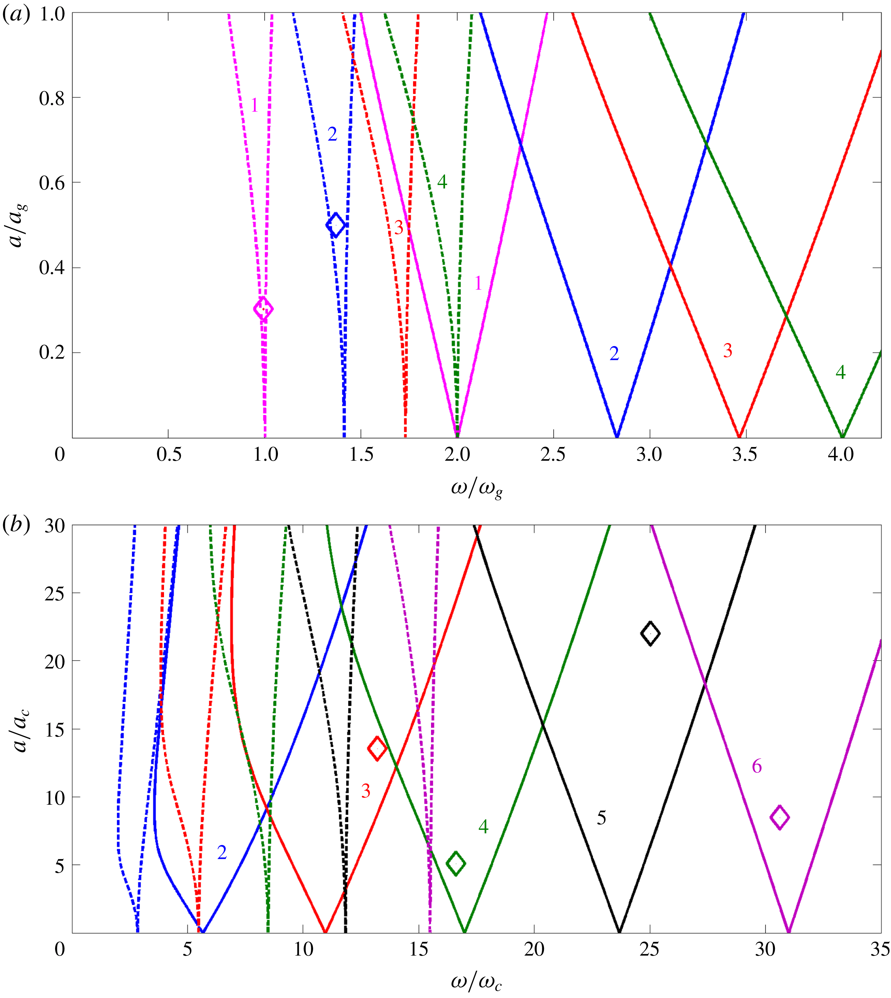
of either infinity or zero. Figure 6 locates the parameter values that we have used for our simulations within the instability tongues for the gravitational or capillary cases, where
 $$\begin{eqnarray}\displaystyle & \displaystyle \unicode[STIX]{x1D714}_{g}^{2}\equiv \frac{g}{R},\quad \unicode[STIX]{x1D714}_{c}^{2}\equiv \frac{\unicode[STIX]{x1D70E}}{\unicode[STIX]{x1D70C}R^{3}}, & \displaystyle\end{eqnarray}$$
 $$\begin{eqnarray}\displaystyle & \displaystyle a_{g}\equiv R\unicode[STIX]{x1D714}_{g}^{2}=g,\quad a_{c}\equiv R\unicode[STIX]{x1D714}_{c}^{2}=\frac{\unicode[STIX]{x1D70E}}{\unicode[STIX]{x1D70C}R^{2}}. & \displaystyle\end{eqnarray}$$
See Ebo-Adou & Tuckerman (Reference Ebo-Adou and Tuckerman2016) for more details on this non-dimensionalization. Because our viscosity is low, the tongues are very close to the inviscid ones; we plot the inviscid tongues for simplicity.
Frequencies were chosen to induce instabilities from
 $\ell =1$
to
 $\ell =6$
, as predicted from linear Floquet theory. In each case, the value of
 $\ell$
from the full three-dimensional nonlinear numerical simulations agreed with the theoretical value.
3 Results
3.1 Case
 $\ell =1$

We begin by presenting the
 $\ell =1$
case in the purely gravitational regime, i.e. in the presence of a constant radial force
 $g\boldsymbol{e}_{r}$
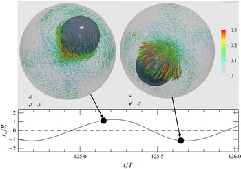
included in the time-periodic force (2.2) and without surface tension. Our simulations of this case exhibit a periodic subharmonic translational motion of the sphere about its original position, as shown in figure 7 and supplementary movie 1 available at https://doi.org/10.1017/jfm.2019.252. This explains why the
 $\ell =1$
case is prohibited for capillary waves: translational motion does not involve deformation of the interface, and so surface tension cannot act as a restoring force. (Note the factor of (
 $\ell -1$
) in formulae (2.11) and (2.13).) Although the drop arrives quite close to the bounding sphere in this simulation, it does not touch it.
As stated by Busse (Reference Busse1975), there is no competition between different patterns in this case. All solutions are obtained by rotation of a single axisymmetric pattern, which is expected to be stable. (The three spherical harmonics
 $Y_{1}^{1},Y_{1}^{0},Y_{1}^{-1}$
are also related by rotation.)
Above: visualization of the
 $\ell =1$
mode for a spherical drop. The drop is displaced alternately to the left and the right. Lengths and colours of arrows indicate the velocity magnitude (in
 $\text{m}~\text{s}^{-1}$
) of the surrounding air. Below: centre of the drop as a function of time. Dots indicate the instants at which the visualizations are drawn. See also supplementary movie 1.

3.2 Case
$\ell =2$

To produce a case in which
 $\ell =2$
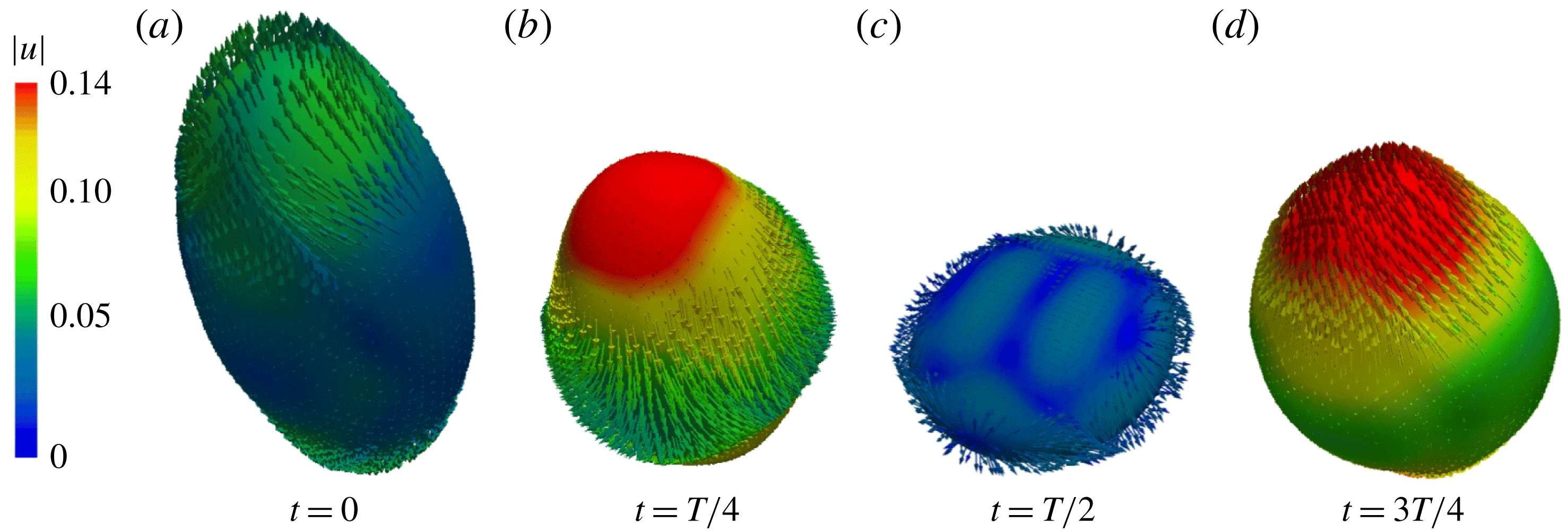
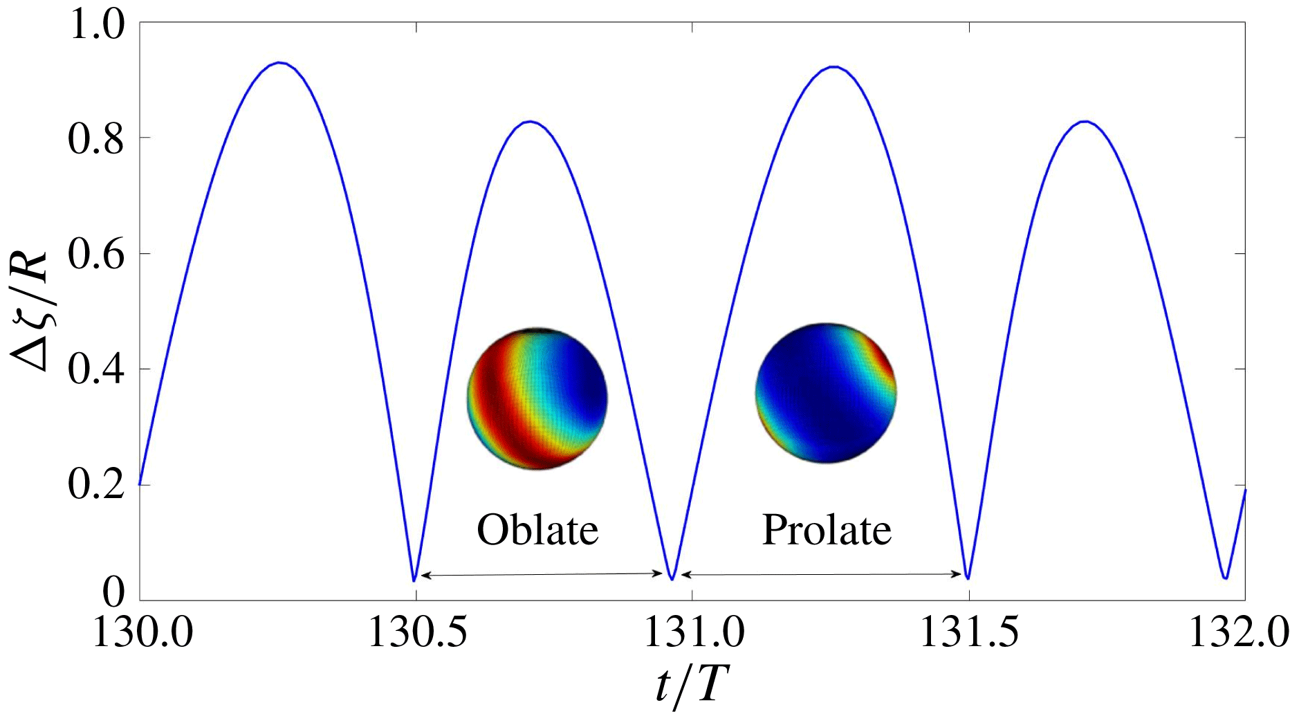
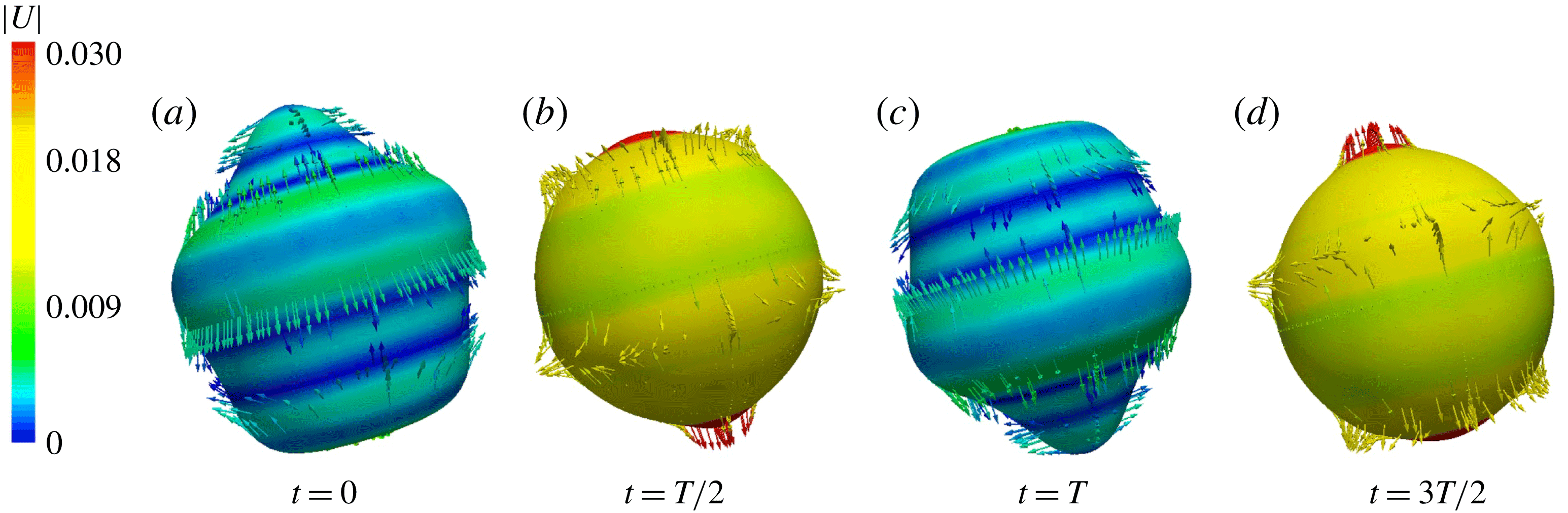
is the dominant mode, we have simulated harmonic oscillations in the gravitational regime. A sequence of figures from our numerical simulations showing the shape and velocity field at the interface is shown in figures 8 and 9, which also shows the velocity field in the outer fluid; see supplementary movie 2. The interface remains axisymmetric, with two principal axes of the same length, and a third of a different length. Figure 8(a) shows a prolate shape, like a rugby ball (the third axis is longer than the other two), while the shape in figure 8(c) is oblate, like a disk (the third axis is shorter). During the prolate phase, the velocity is directed in the polar direction, while during the oblate phase it is directed in the equatorial direction. At maximum deformation, the velocity changes direction, so that the magnitude of the velocity is lowest when the surface is most deformed and highest when it is least deformed. Because the interface is opaque, velocity vectors directed inwards cannot be seen.
Figure 10 shows the amplitude
 $|\unicode[STIX]{x1D701}_{max}-\unicode[STIX]{x1D701}_{min}|$
as a function of time. The prolate and oblate configurations are represented by higher and lower maximum values of
 $|\unicode[STIX]{x1D701}_{max}-\unicode[STIX]{x1D701}_{min}|$
, respectively. Oblate-to-prolate oscillations have been studied extensively (Trinh & Wang Reference Trinh and Wang1982; Tsamopoulos & Brown Reference Tsamopoulos and Brown1983; Patzek et al.
Reference Patzek, Benner, Basaran and Scriven1991). These authors observe that the drop spends a longer time in the prolate than in the oblate configuration, which agrees with our observation that the drop spends approximately 53 % of each period in the prolate configuration. This is explained by the combination of two facts: the restoring force is governed by the pressure at the curved surface, and the poles cover a smaller surface than the equator. The prolate rugby-ball-like form, with high curvature at the poles, is therefore subjected to a smaller restoring force than the oblate disk-like form, with high curvature at the equator. Hence it takes more time for the drop to return from the prolate to the spherical shape than it takes to return from the oblate shape.
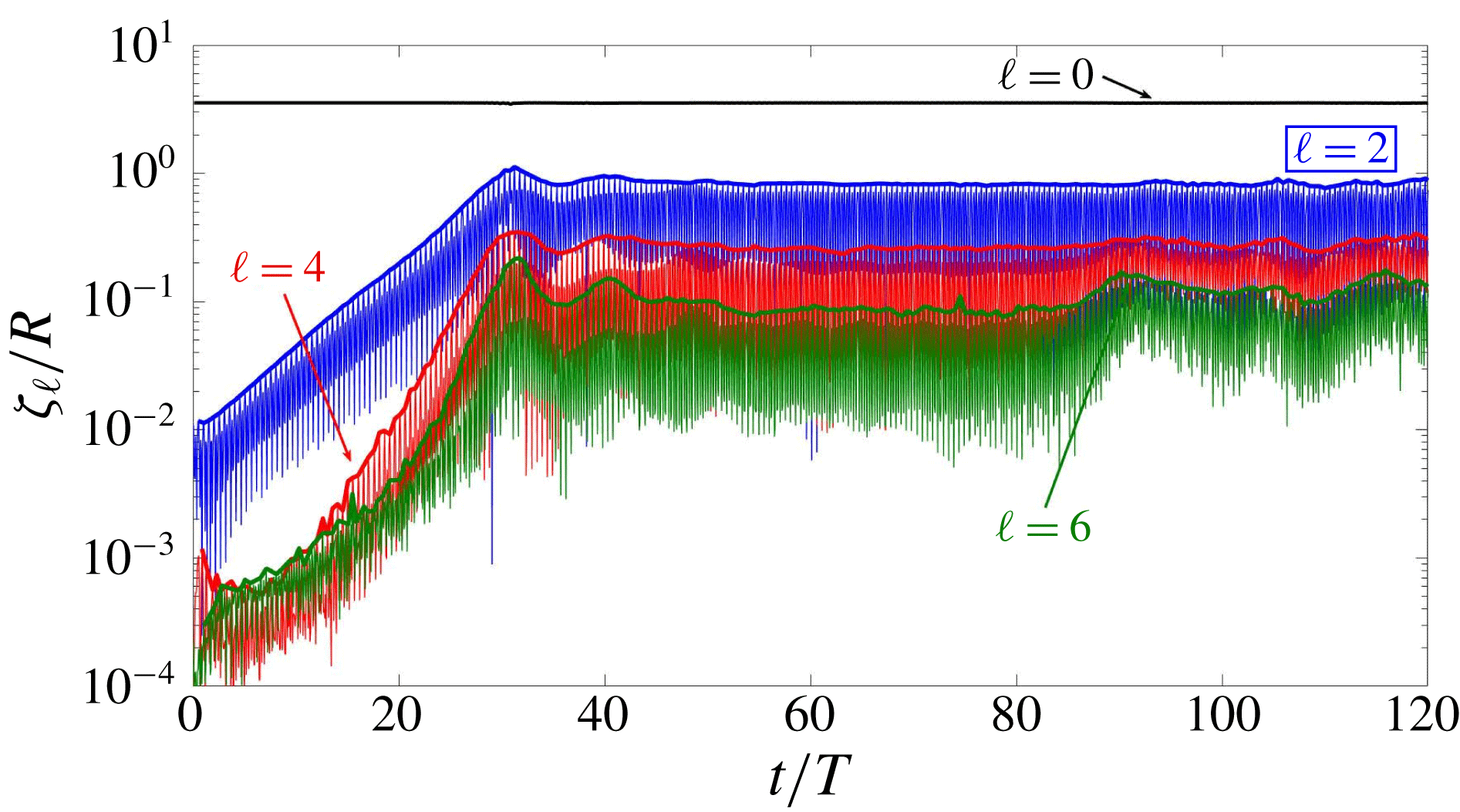
In figures 11 and 12, we present the spherical harmonic coefficients of the interface height
 $\unicode[STIX]{x1D701}(\unicode[STIX]{x1D703},\unicode[STIX]{x1D719},t)$
, calculated from equations (2.8) and (2.9) as explained in § 2.5. Figure 11 shows the time evolution of
 $\unicode[STIX]{x1D701}_{\ell }$
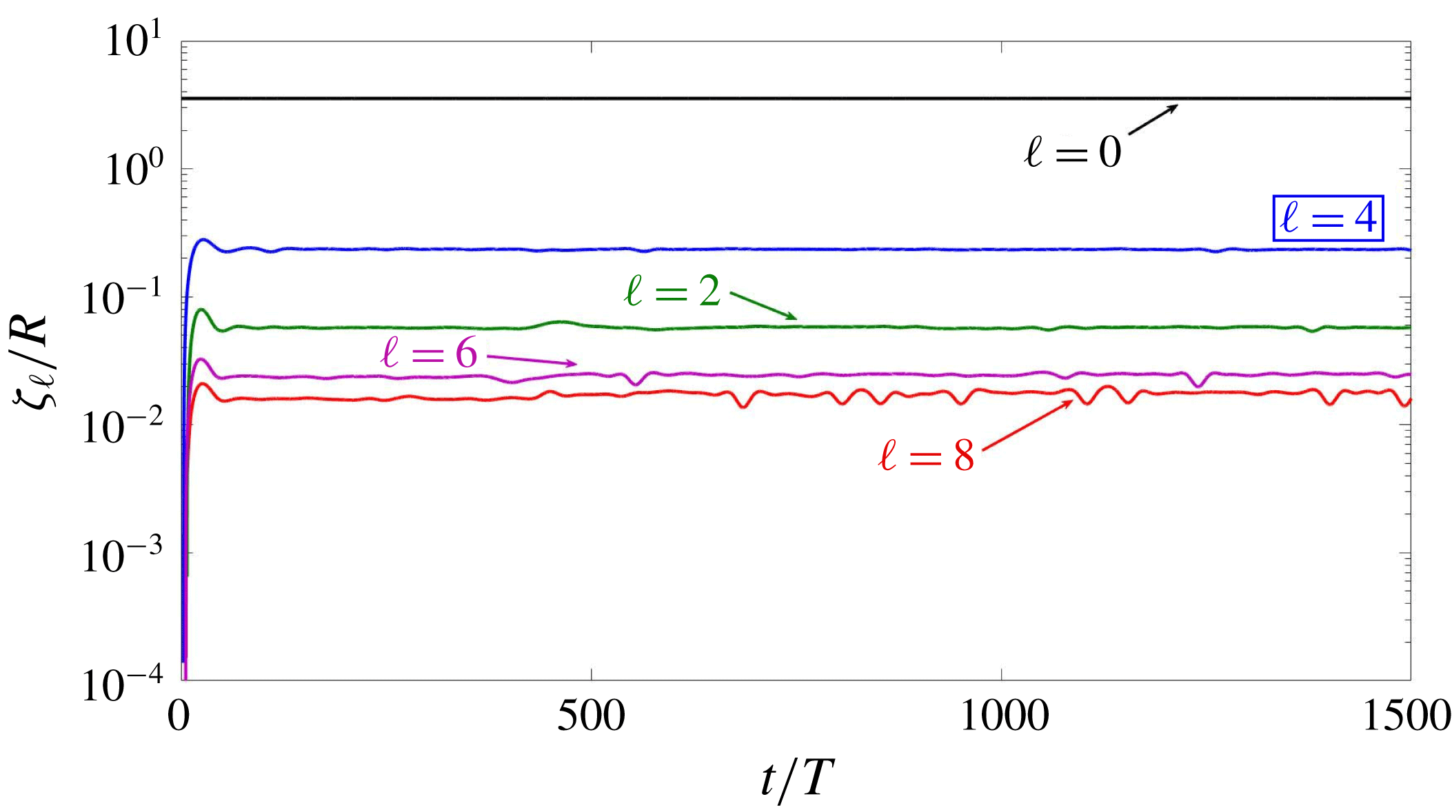
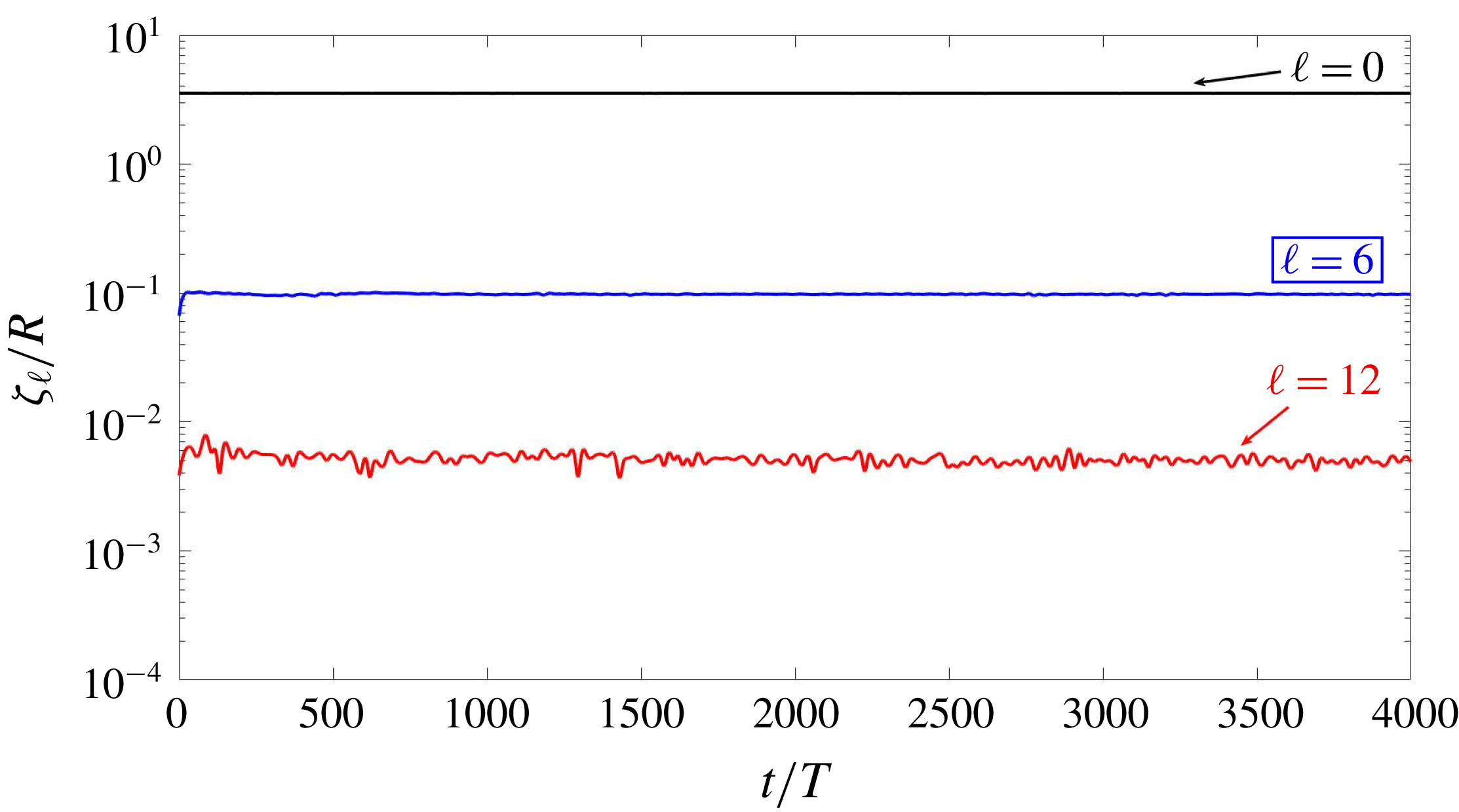
, defined in (2.9). Its most visible feature is its rapid oscillation. In order to examine the dynamics over time scales much larger than the forcing period
 $T$
, we extract the envelope of each
 $\unicode[STIX]{x1D701}_{\ell }$
, as shown by the bold curves in figure 11. The variation of
 $\unicode[STIX]{x1D701}_{0}$
cannot be seen on this scale, since it is
 $\sqrt{4\unicode[STIX]{x03C0}}$
times the mean radius, which should be nearly constant due to incompressibility. Although
 $\ell =2$
is the dominant non-zero spherical wavenumber for this case, other even
 $\ell$
(multiples of 2) are also present, generated by nonlinear interactions. Standard bifurcation theory predicts that the growth rate of the harmonic
 $n\ell$
should be approximately
 $n$
times that of
 $\ell$
, shown here by the fact that
 $\unicode[STIX]{x1D701}_{4}$
grows approximately twice as quickly as
 $\unicode[STIX]{x1D701}_{2}$
.
Although we began our simulations by perturbing the sphere with an axisymmetric initial condition, proportional to
 $Y_{2}^{0}$
, the drop orientation quickly tilts away from the
 $z$
axis, acquiring components with
 $m\neq 0$
while remaining axisymmetric about its own axis. The symmetry axis continues to rotate and to oscillate periodically, manifested by the behaviour of components
 $m=0$
, 1 and 2, shown in figure 12. We have also obtained prolate–oblate oscillations in simulations (not presented here) of subharmonic capillary waves with the same axisymmetric initial condition.
Drop interface and velocity field for the
 $\ell =2$
prolate–oblate pattern of gravitational harmonic waves over one response period
 $T$
. During the prolate phase, the velocity is directed in the polar direction, while during the oblate phase it is directed in the equatorial direction. Colours indicate the magnitude of the velocity (in
 $\text{m}~\text{s}^{-1}$
), which is maximal when the surface is least deformed and minimal where it is most deformed. Only outward-pointing velocity vectors are shown; those pointing inwards are hidden by the opaque surface of the drop.

Same as figure 8 but from a slightly different perspective and showing the outer bounding sphere and the velocity field in the outer fluid. See also supplementary movie 2.

Time series of the interface amplitude
 $|\unicode[STIX]{x1D701}_{max}-\unicode[STIX]{x1D701}_{min}|$
for
 $\ell \,=\,2$
. Insets show the projection of the height
 $\unicode[STIX]{x1D701}(\unicode[STIX]{x1D703},\unicode[STIX]{x1D719})$
on the sphere. Prolate and oblate configurations have higher and lower maximum values of
 $|\unicode[STIX]{x1D701}_{max}-\unicode[STIX]{x1D701}_{min}|$
, respectively. The drop spends approximately 53 % of each period in the prolate configuration.

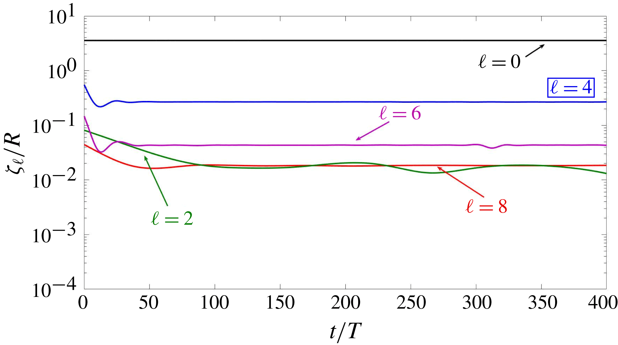
Time series of
 $\ell$
components for a pattern whose dominant mode is
 $\ell =2$
(indicated by the boxed label). All multiples of
 $\ell =2$
are present, as well as
 $\ell =0$
, which is the constant average radius. Long-time evolution is visualized by envelopes (bold curves) of the rapidly oscillating time series. The growth rate of component
 $\unicode[STIX]{x1D701}_{4}$
is approximately twice that of
 $\unicode[STIX]{x1D701}_{2}$
.

Time series of
 $m$
components for an
 $\ell \,=\,2$
pattern. Initially, the drop is axisymmetric and the only component is
 $m=0$
. The drop remains axisymmetric, but its axis of symmetry tilts away from the
 $z$
axis and continues to rotate and oscillate, as manifested by the alternating dominance of
 $m=0$
, 1, and 2.

Busse (Reference Busse1975) and Chossat et al. (Reference Chossat, Lauterbach and Melbourne1991) show that the only allowed solution for
 $\ell =2$
is axisymmetric and unstable at onset. In our simulations, which are far from onset, we observe an axisymmetric pattern whose orientation continually changes.
3.3 Case
$\ell =3$

For
 $\ell =3$
, there exist solutions with three possible symmetries: axisymmetric,
 $D_{6}$
, and tetrahedral. Either the
 $D_{6}$
or the tetrahedral solution can be stable at onset (Busse Reference Busse1975; Chossat et al.
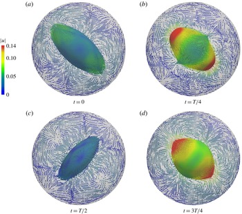
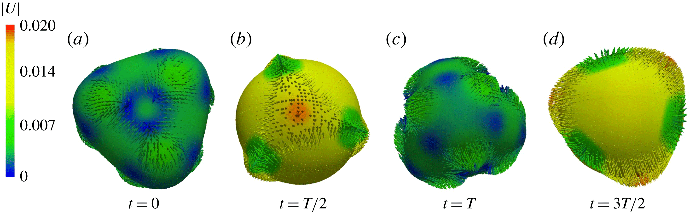
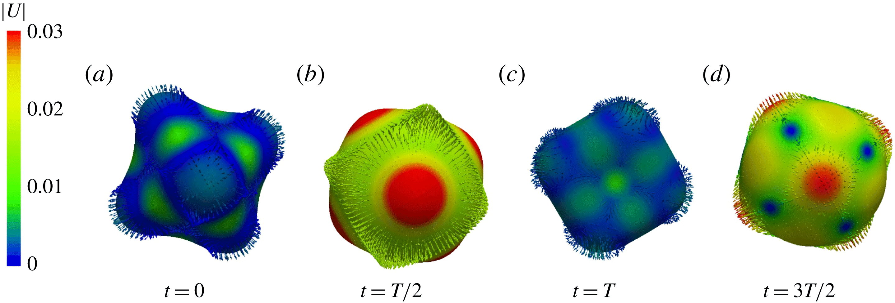
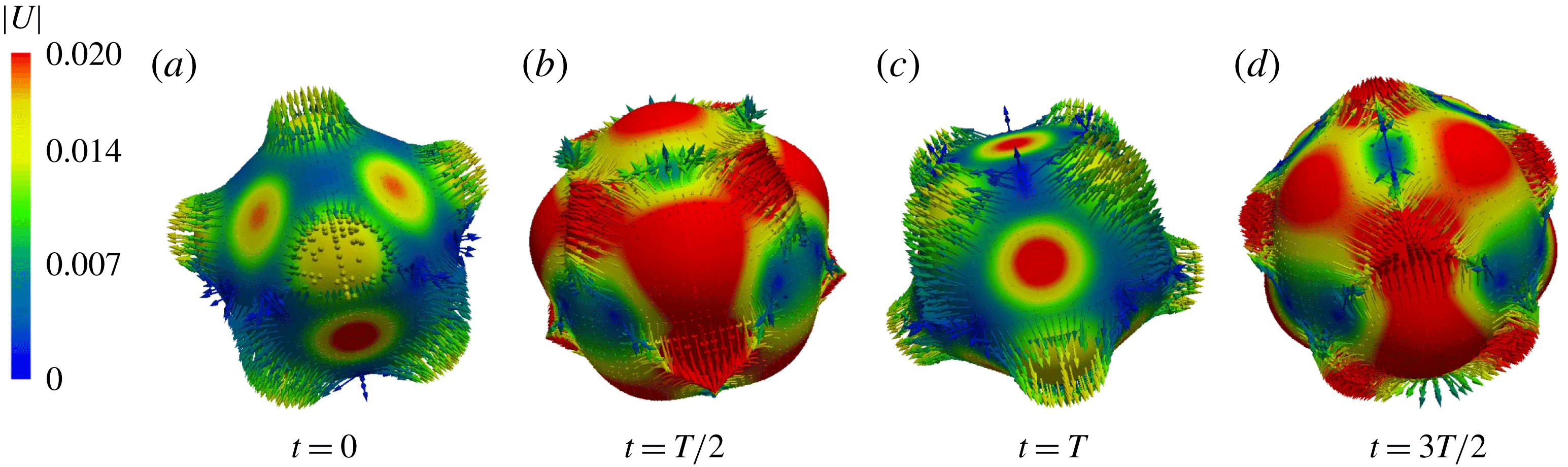
Reference Chossat, Lauterbach and Melbourne1991). Starting from an axisymmetric initial condition, our solution for this case rapidly develops tetrahedral symmetry, as can be seen in figure 13 and supplementary movie 3, which show subharmonic capillary oscillations. Over a half oscillation period, the tetrahedron in figure 13(a) reverses its orientation, as shown in figure 13(c), since this polyhedron is self-dual. The initial condition is axisymmetric, but the same behaviour is seen starting from a sphere slightly perturbed by numerical noise.
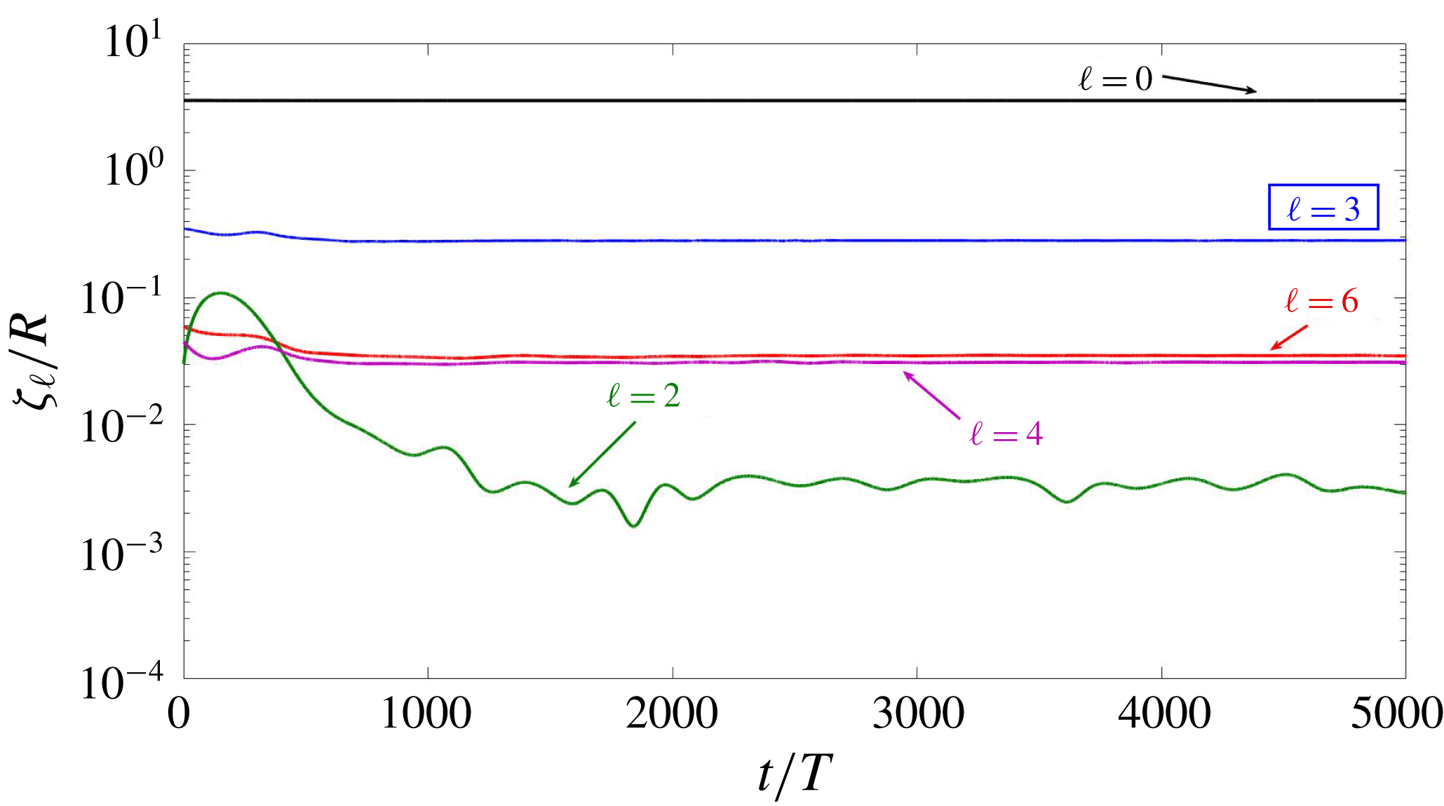
The pattern contains components other than
 $\ell =3$
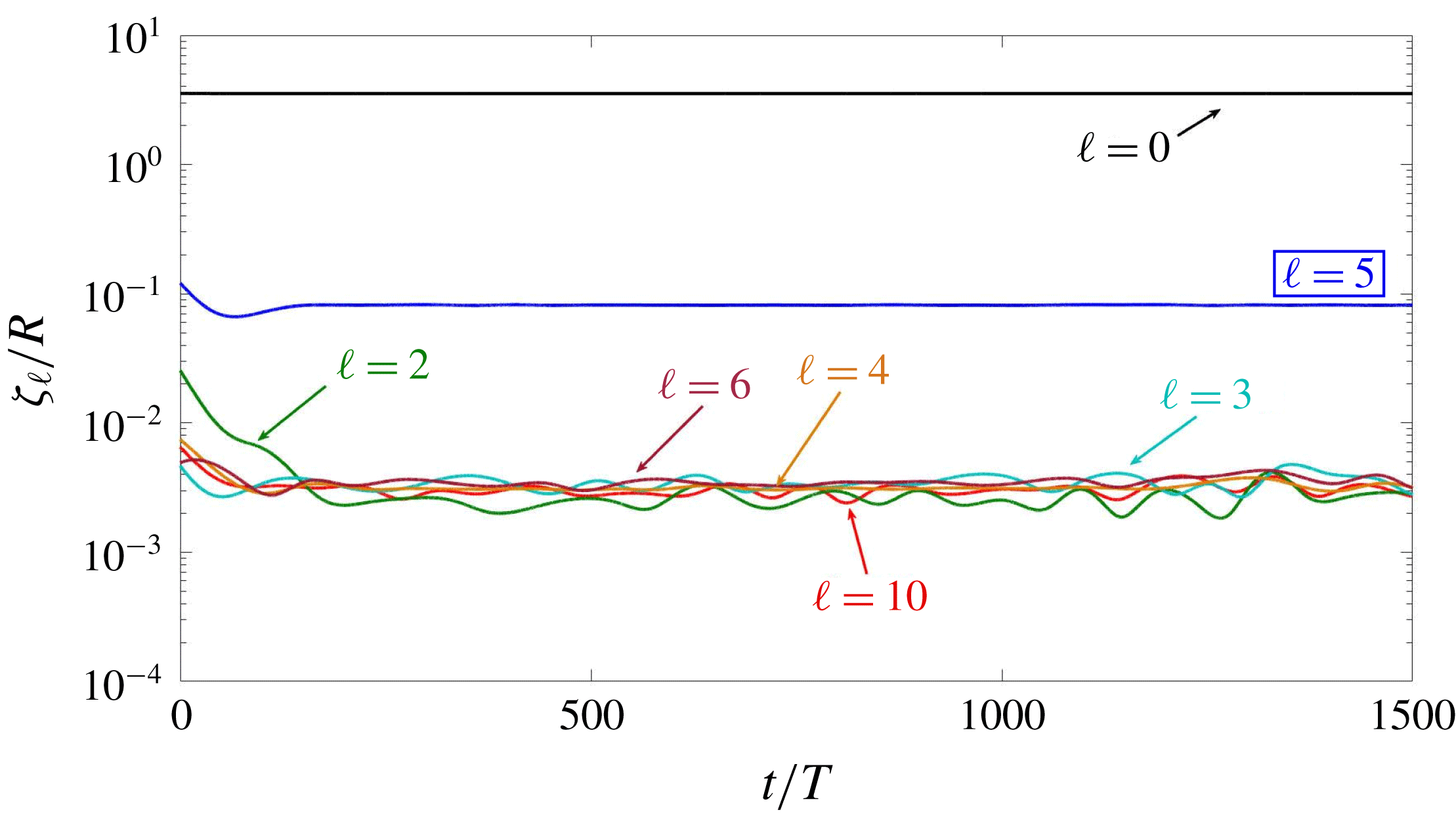
and its harmonics, as illustrated in figure 14. In particular, an important
 $\ell =4$
component is present, of approximately the same magnitude as the first harmonic
 $\ell =6$
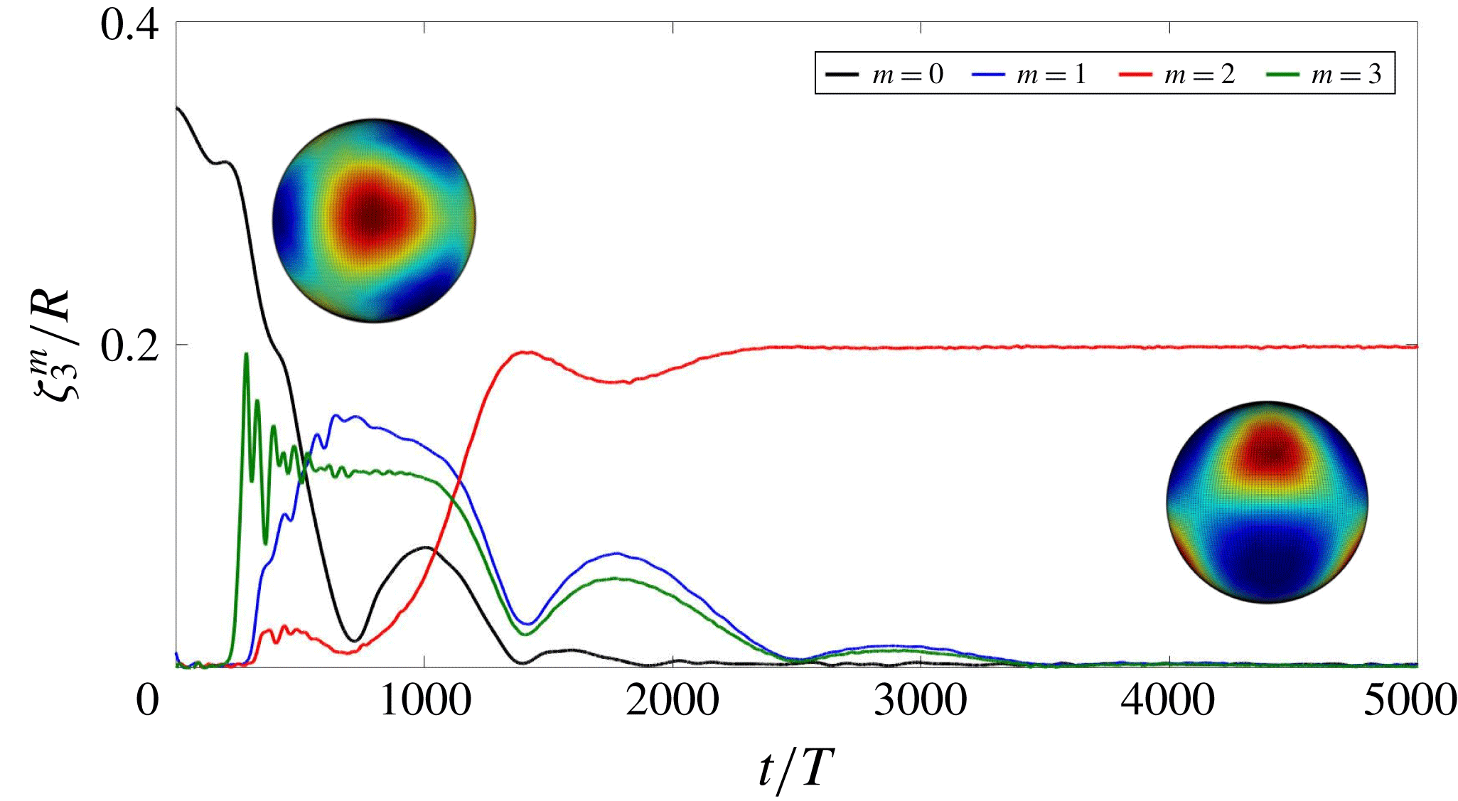
. Figure 15 shows the rapid progression from the axisymmetric initial condition to a tetrahedral one, as component
 $m=0$
falls and the other components rise. There follows a long phase during which the orientation of the tetrahedal pattern varies. Eventually, by
 $t/T\approx 2000$
, the tetrahedron aligns with the
 $z$
axis, with only
 $m=2$
remaining; recall from equation (2.14b
) that
 $Y_{3}^{2}+\text{c.c.}$
corresponds to a tetrahedron aligned with the
 $z$
-axis (Busse Reference Busse1975).
3.4 Case
$\ell =4$

When
 $\ell =4$
, bifurcation theory predicts two possible solutions at onset (Busse Reference Busse1975; Chossat et al.
Reference Chossat, Lauterbach and Melbourne1991), with axisymmetric or cubic symmetry, produced by a transcritical bifurcation. Neither branch is stable at onset but the cubic solution is the preferred one (Busse Reference Busse1975; Matthews Reference Matthews2003). We have been able to produce patterns of both kinds by starting with initial conditions which are axisymmetric or cubic
 $$\begin{eqnarray}\unicode[STIX]{x1D701}-R\propto \sqrt{7}Y_{4}^{0}+\sqrt{5}Y_{4}^{4}+\text{c.c.}\end{eqnarray}$$
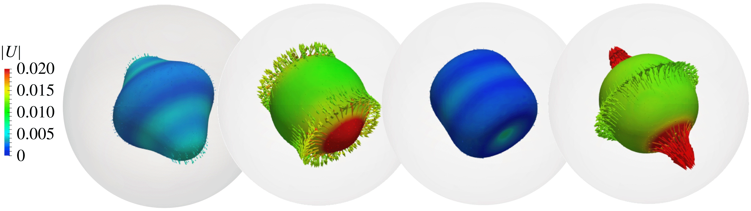
Visualizations of our numerical simulations of subharmonic capillary oscillations with cubic symmetry are shown in figure 16 and supplementary movie 4a. The pattern oscillates between resembling a cube, with six square faces, of which three meet at each vertex, and its dual, the octahedron with eight equilateral triangles, four of which meet at each corner.
Figure 17 shows that, in addition to
 $\ell =4$
and its harmonics, the
 $\ell$
wavenumber spectrum contains a large
 $\ell =6$
component, as well as modes resulting from interactions between the
 $\ell =4$
and
 $\ell =6$
families. The pattern is aligned with the numerical domain, with two faces or minima (for the cube) or two vertices or maxima (for the octahedron) located at the north and south poles. With this alignment, the cubic solution is expected to be a sum of
 $Y_{4}^{0}$
and
 $Y_{4}^{\pm 4}$
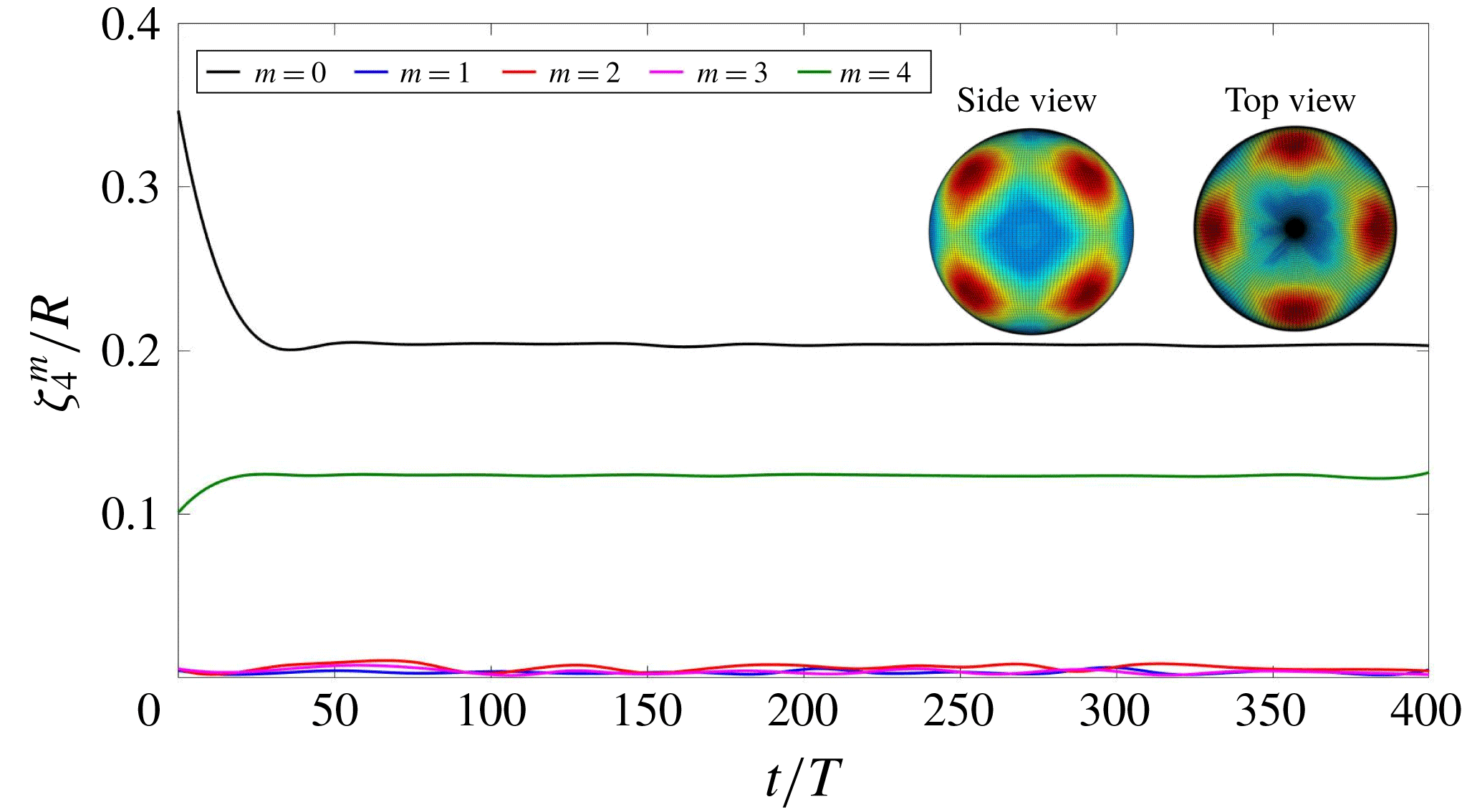
. Indeed figure 18 shows that
 $\unicode[STIX]{x1D701}_{4}^{0}$
and
 $\unicode[STIX]{x1D701}_{4}^{4}$
are dominant and constant. We have also obtained a cubic pattern in simulations (not presented here) of harmonic gravitational waves with a perturbed spherical initial condition and a resolution of
 $256^{3}$
.
From an axisymmetric initial condition, the solution remains axisymmetric over the time of our simulation, but develops a tilting and rotating axis of symmetry, as was the case for
 $\ell =2$
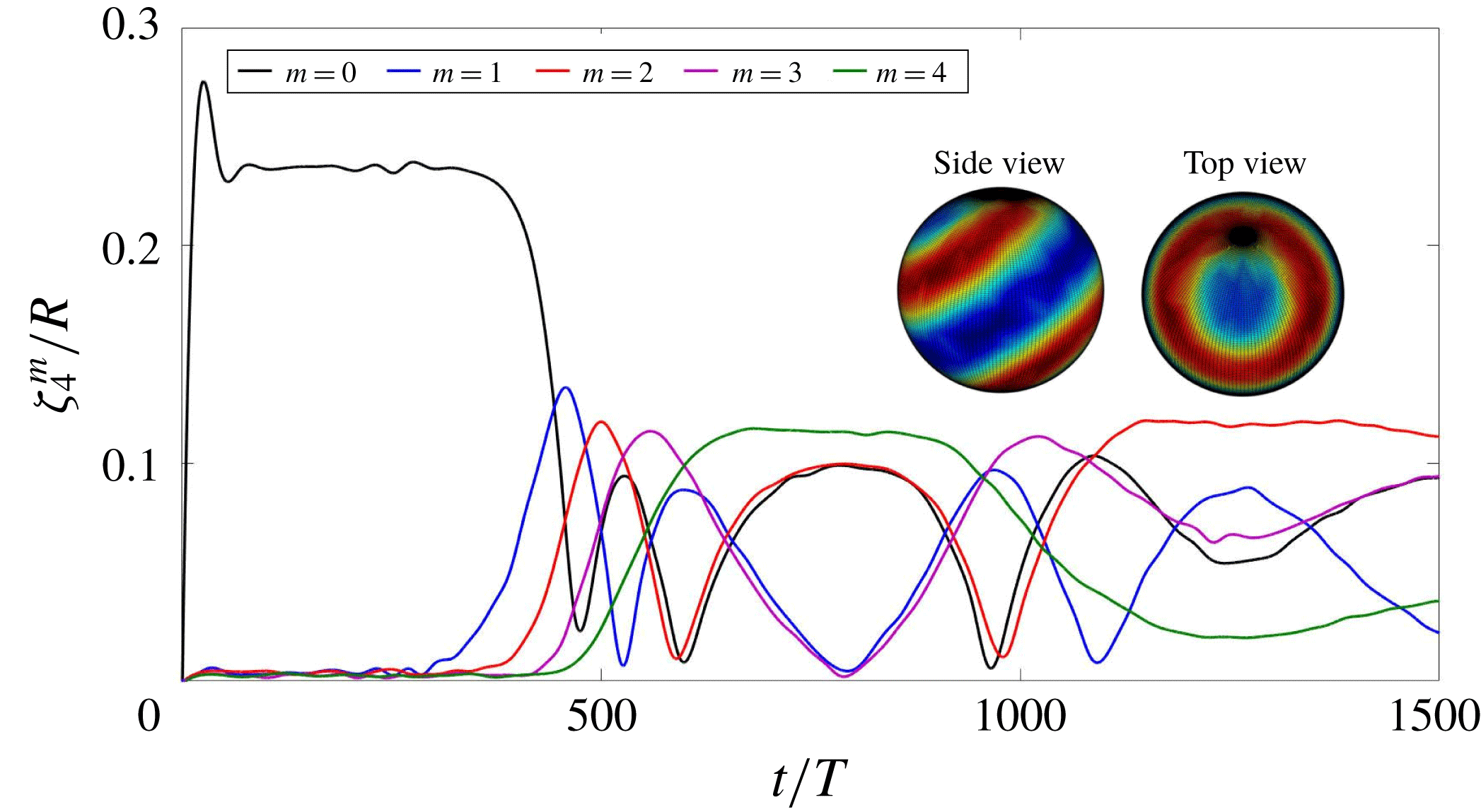
. Visualizations of this state are shown in figure 19 and supplementary movie 4b. Figure 20 shows the evolution of the amplitudes of the various
 $\ell$
modes. We observe that
 $\unicode[STIX]{x1D701}_{2}$
is higher (a feature we have observed whenever a pattern is axisymmetric) and
 $\unicode[STIX]{x1D701}_{6}$
is lower than was the case for the cubic solution. The oscillatory behaviour of the various
 $m$
modes in figure 21 are manifestations of the fact that the axis of symmetry rotates, as in figure 12.
3.5 Case
$\ell =5$

The theoretical analysis of the
 $\ell =5$
case is the most complicated of those surveyed here (Busse & Riahi Reference Busse and Riahi1982; Riahi Reference Riahi1984), since it leads to eight allowed solutions with different symmetries (Chossat et al.
Reference Chossat, Lauterbach and Melbourne1991). We find two of these solutions in our simulations, one as a short-lived unstable equilibrium and the other as a long-term asymptotic state.
Drop interface and corresponding velocity field for the
 $\ell =3$
tetrahedral pattern seen in subharmonic capillary waves over one reponse period
 $2T$
. Colours indicate the magnitude of the velocity (in
 $\text{m}~\text{s}^{-1}$
), which is maximal when the surface is least deformed and minimal where it is most deformed. Only outward-pointing velocity vectors are shown; those pointing inwards are hidden by the opaque surface of the drop. See also supplementary movie 3.

Time series of
 $\ell$
components for a pattern whose dominant mode is
 $\ell =3$
. The amplitude of mode
 $\ell =4$
is very close to that of the second harmonic
 $\ell =6$
.

Time series of
 $m$
components for an
 $\ell =3$
pattern. Initially the drop is axisymmetric. By
 $t/T\approx 450$
, the
 $m=3$
component has risen and the shape is tetrahedral and tilted with respect to the
 $z$
axis. As the
 $m=2$
component increases, the pattern aligns with the
 $z$
axis.

Drop interface and velocity field for the
 $\ell =4$
cubic pattern seen in subharmonic capillary waves over one reponse period
 $2T$
. The interface oscillates between (a) an octahedron, with six maxima, and (c) a cube, with eight maxima. Colours indicate the magnitude of the velocity (in
 $\text{m}~\text{s}^{-1}$
), which is maximal (minimal) when the surface is least (most) deformed. Only outward-pointing velocity vectors are shown. See also supplementary movie 4a.

Time series of
 $\ell$
components for a pattern whose dominant mode is
 $\ell =4$
when the initial condition is cubic. The spectrum also contains important
 $\ell =2$
and
 $\ell =6=4+2$
components.

Time series of
 $m$
components for an
 $\ell =4$
pattern when the initial condition is cubic. The pattern is stable and consists of a superposition of modes
 $m=0$
and
 $m=4$
, i.e. it is cubic and aligned with the
 $z$
axis.

Drop interface and velocity field for the
 $\ell =4$
axisymmetric pattern seen in subharmonic capillary waves at various phases during one response period
 $2T$
. The interface oscillates between a cylinder and a top-shaped object. Each drop is shown inside its spherical domain. Colours indicate the magnitude of the velocity (in
 $\text{m}~\text{s}^{-1}$
), which is maximal (minimal) when the surface is least (most) deformed. Only outward-pointing velocity vectors are shown. See also supplementary movie 4b.

Time evolution of amplitude of different
 $\ell$
components when the dominant wavenumber is
 $\ell =4$
and the initial condition is axisymmetric. The spectrum also contains important
 $\ell =2$
and
 $\ell =6=4+2$
components.

Time series of
 $m$
components for an
 $\ell =4$
pattern when the initial condition is axisymmetric. The pattern remains axisymmetric, but its axis changes its orientation in time.

Drop interface and corresponding velocity field for the transient axisymmetric
 $\ell =5$
pattern seen in subharmonic capillary waves over one reponse period
 $2T$
. Colours indicate the magnitude of the velocity (in
 $\text{m}~\text{s}^{-1}$
), which is maximal (minimal) when the surface is least (most) deformed. Only outward-pointing velocity vectors are shown. See also supplementary movie 5.

Drop interface and corresponding velocity field for the final
 $\ell =5$
pattern with
 $D_{4}$
symmetry. See also supplementary movie 5.

Starting from an initial condition which is an axisymmetric perturbation of the sphere, the solution quickly equilibrates to axisymmetric oscillations which are shown in figure 22. The solution is then replaced by another solution with
 $D_{4}$
symmetry, shown in figure 23. See supplementary movie 5. In the
 $D_{4}$
solution, the upper hemisphere contains four patches of outward (inward) flow, and the lower hemisphere contains four similar patches, located at longitudes which are halfway between those of the patches of the upper hemisphere. This pattern corresponds to the preferred solution called
 $\boldsymbol{F}$
by Riahi (Reference Riahi1984):
 $$\begin{eqnarray}\unicode[STIX]{x1D701}-R\propto \sqrt{3}Y_{5}^{0}+\sqrt{5}Y_{5}^{4}+\text{c.c.}\end{eqnarray}$$
The spectra in
 $\ell$
and
 $m$
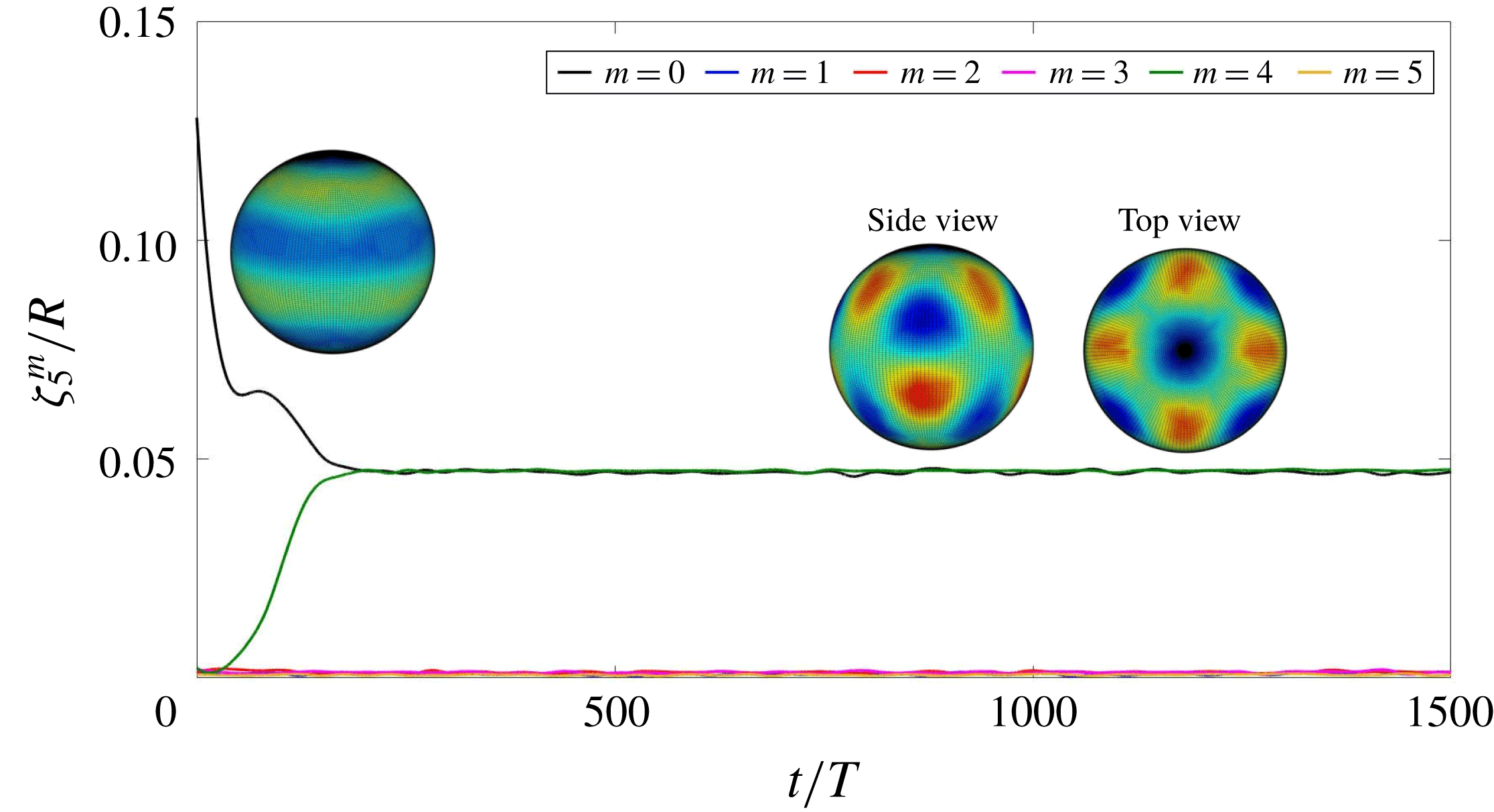
are shown in figures 24 and 25. Because the pattern remains aligned with the
 $z$
axis, the transition from the axisymmetric pattern to (3.2) can be tracked by following the different
 $m$
modes, as is done in figure 25. The initial plateau in
 $\unicode[STIX]{x1D701}_{5}^{0}$
indicates that the axisymmetric phase of the oscillations shown in figure 22 comprises a solution, albeit unstable, of our system. (This is accompanied in figure 24 by a brief slowing of the decay of the
 $\ell =2$
mode which is present in all of our nonlinear axisymmetric solutions.) The subsequent decrease in
 $\unicode[STIX]{x1D701}_{5}^{0}$
is accompanied by an increase in
 $\unicode[STIX]{x1D701}_{5}^{4}$
, which together comprise the stable solution with
 $D_{4}$
symmetry.
Time series of
 $\ell$
components for a pattern whose dominant mode is
 $\ell =5$
when the initial condition is axisymmetric. Many components are present, in addition to the expected multiples of 5.

Time series of
 $m$
components for an
 $\ell =5$
pattern. An initially axisymmetric pattern with
 $m=0$
briefly equilibrates and is then replaced by a
 $D_{4}$
pattern, which is a superposition of
 $m=0$
and
 $m=4$
.

3.6 Case
$\ell =6$

We compute subharmonic capillary oscillations for
 $\ell =6$
. For
 $\ell =6$
, there exist four possible solutions: axisymmetric, six-fold symmetric (
 $D_{6}$
), octahedral and icosahedral. Of these, the icosahedral solution is preferred near threshold, via a maximization argument (Busse Reference Busse1975) or a stability argument (Matthews Reference Matthews2003). With this in mind, we use as an initial condition an icosahedral perturbation of the sphere (Busse Reference Busse1975):
 $$\begin{eqnarray}\unicode[STIX]{x1D701}-R\propto \sqrt{11}Y_{6}^{0}+\sqrt{14}Y_{6}^{5}+\text{c.c.}\end{eqnarray}$$
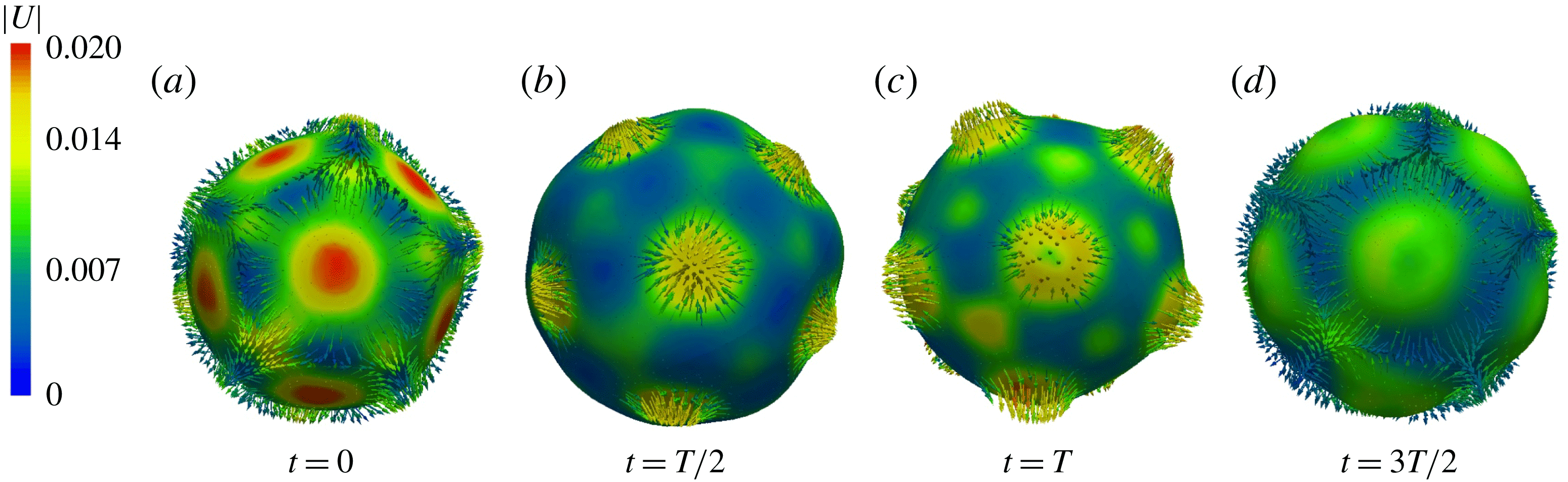
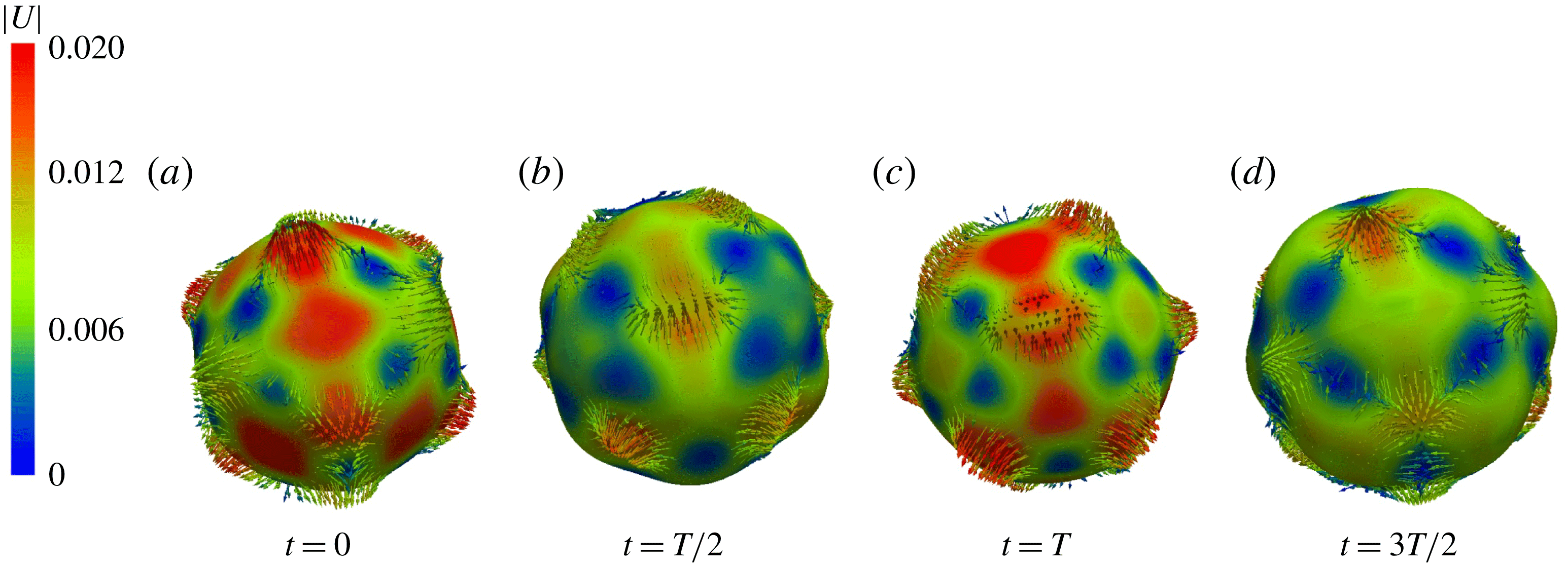
Figure 26 shows the icosahedral/dodecahedral oscillations during the first phase of the simulation, with a clear five-fold symmetry; see also supplementary movie 6. Figure 26(a) resembles a dodecahedron, i.e. pentagons which meet in sets of three at the vertices, while 26(c) resembles an icosahedron, i.e. triangles which meet in sets of five at the vertices. Further evolution leads to a second phase of the solution, shown in figure 27, which oscillates between a cube and its dual, an octahedron. Indeed, simulations from a spherical initial condition (perturbed by its discrete representation on a triangular mesh) also led directly to the cubic/octahedral solution.
Drop interface and corresponding velocity field for the
 $\ell =6$
transient pattern with icosahedral symmetry of subharmonic capillary waves over one reponse period
 $2T$
. Colours indicate the magnitude of the velocity (in
 $\text{m}~\text{s}^{-1}$
), which is maximal (minimal) when the surface is least (most) deformed. Only outward-pointing velocity vectors are shown. See also supplementary movie 6.

Drop interface and corresponding velocity field for the
 $\ell =6$
transient pattern with cubic symmetry.

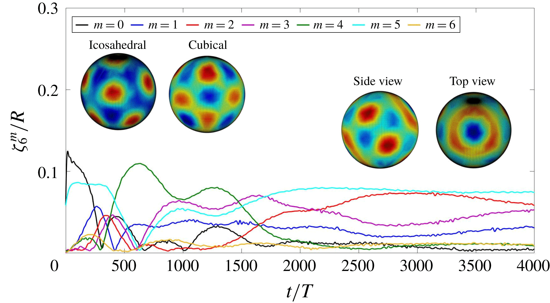
Figure 28 shows the time evolution of the spectrum in
 $\ell$
, while figure 29 shows the time evolution of the most important
 $m$
modes associated with
 $\ell =6$
. The icosahedral pattern, consisting of modes
 $m=0$
and
 $m=5$
, quickly tilts away from the
 $z$
axis and by
 $t/T\approx 300$
is replaced by a cubic pattern, whose dominant mode is
 $m=4$
. The subsequent increase in
 $m=3$
is associated with the tilting of the cubic pattern away from the
 $z$
axis. Eventually, however, the solution shifts to the pattern shown in the rightmost insets of figure 29, which is neither icosahedral nor cubic.
4 Discussion
Using the parallel front-tracking code BLUE, we have been able to simulate the spherical Faraday problem and thereby to produce patterns with all spherical harmonic wavenumbers between
 $\ell =1$
and
 $\ell =6$
. We have simulated both gravitational and capillary waves, in both the harmonic regime and the more usual subharmonic regime.
Time evolution of the amplitudes of modes with different
 $\ell$
values when the dominant mode is
 $\ell =6$
.

Time series of
 $m$
components for an
 $\ell =6$
pattern. From an icosahedral initial condition composed of modes
 $m=0$
and
 $m=5$
, the pattern tilts away from the
 $z$
axis and by
 $t/T\approx 300$
acquires cubic symmetry with dominant mode
 $m=4$
. The subsequent increase in mode
 $m=3$
at
 $t/T\approx 800$
is associated with tilting of the orientation of the cubical pattern away from the
 $z$
axis. Insets show projections of the initial icosahedral pattern, the subsequent cubic pattern, and the solution at later times, which is neither of these.

Our simulations agree in most cases with two types of theory. First, the spherical harmonic wavenumber
 $\ell$
obtained in each case agrees with the results of Floquet analysis, presented in Ebo-Adou & Tuckerman (Reference Ebo-Adou and Tuckerman2016) and in figure 6. Second, the interface shapes we observe are readily interpreted using the theory of pattern formation on the sphere (Busse Reference Busse1975; Busse & Riahi Reference Busse and Riahi1982; Ihrig & Golubitsky Reference Ihrig and Golubitsky1984; Riahi Reference Riahi1984; Golubitsky et al.
Reference Golubitsky, Stewart and Schaeffer1988; Chossat et al.
Reference Chossat, Lauterbach and Melbourne1991; Matthews Reference Matthews2003). For
 $\ell =1$
and
 $\ell =2$
, only one type of pattern is possible, and that is the one we observe. For our vibrating drop, the
 $\ell =1$
‘pattern’ is manifested as a back-and-forth motion of the spherical drop, while the
 $\ell =2$
pattern alternates between an oblate and a prolate spheroid. For
 $\ell =3$
, we observe a tetrahedral pattern, one of the two solutions predicted to be stable (out of the three which can exist), while for
 $\ell =4$
, depending on the initial conditions, we observe both of the possible solutions, a cubic/octahedral or an axisymmetric pattern. For
 $\ell =5$
, we observe an unstable axisymmetric and a stable
 $D_{4}$
pattern. These are two of the eight possible solutions;
 $D_{4}$
is one of those which can be stable at onset. For
 $\ell =6$
, an initially icosahedral solution makes a transition to a cubic/octahedral pattern, which is succeeded by a solution with neither symmetry. It is surprising to find such good agreement with theory given the differences with our configuration mentioned in the introduction, i.e. the fact that our patterns are oscillatory rather than steady and that our parameters are far above threshold. A complete study of each of these cases, varying the forcing amplitude from threshold to higher values, would be desirable. Another crucial issue, both empirical and mathematical, is the possible difference between the harmonic and subharmonic regimes in each of the cases.
An important avenue of exploration that has arisen in our study is that of the long-term dynamics. The
 $\ell =2$
(prolate–oblate) and
 $\ell =4$
(axisymmetric) show the drop tumbling into and out of alignment with the coordinate system, as illustrated in figures 12 and 21. The
 $\ell =3$
(tetrahedral) and
 $\ell =6$
(cubic/octahedral) oscillations in figures 15 and 29 also show very long phases (2000 or more forcing periods
 $T$
) during which the orientation continues to change. Another case in which very long-term Faraday-wave dynamics has been found is that of hexagonal waves in a minimal domain (Périnet et al.
Reference Périnet, Juric and Tuckerman2012). To the best of our knowledge, there exists no explanation of such long-term dynamics in terms of pattern formation, fluid dynamics, or any other kind of theory.
We have demonstrated the feasibility of well-resolved numerical simulation of the spherical version of the Faraday instability over extremely long times. We believe that the Faraday problem serves as a rigorous proving ground for numerical interface techniques. The wide variety of drop shapes and their detailed patterns simulated here demonstrate the necessity and advantages of using high-fidelity numerical techniques developed for accurately computing two-phase flows and free surfaces, particularly where precise volume conservation, interface advection and calculation of surface tension forces are fundamental. We hope that this work on the spherical Faraday instability can open up new possibilities in the study of pattern formation and that the numerical code can serve as a useful tool in the exploration of this rich dynamical system. In addition, we believe that the results obtained here serve both to validate the techniques implemented in BLUE and also to provide encouragement in applying the code to two-phase flow scenarios in highly nonlinear regimes.
Acknowledgements
This work was performed using high-performance computing resources provided by the Institut du Developpement et des Ressources en Informatique Scientifique (IDRIS) of the Centre National de la Recherche Scientifique (CNRS), coordinated by GENCI (Grand Equipement National de Calcul Intensif) through grant nos A0042B06721 and A0042A01119. L.S.T. acknowledges support from the Agence Nationale de la Recherche (ANR) through the TRANSFLOW project. This research was supported by Basic Science Research Program through the National Research Foundation of Korea (NRF) funded by the Ministry of Education (no. 2017R1D1A1B03028518).
Supplementary movies
Supplementary movies are available at https://doi.org/10.1017/jfm.2019.252.