



1. Introduction
When two fluids of different densities, separated by a perturbed interface, are continuously accelerated from the less dense to the denser one, vorticity is baroclinically deposited by the misalignment between local pressure and density gradients. The vorticity drives sustained growth of interface perturbations, known as Rayleigh–Taylor instability (RTI) (Rayleigh Reference Rayleigh1883; Taylor Reference Taylor1950). Generally, RTI begins with a linear stage characterised by exponential growth, followed by a nonlinear stage where large-scale finger structures of bubbles (light fluids penetrating heavy fluids) and spikes (heavy fluids penetrating light fluids) emerge. During the early nonlinear stage, referred to as the quasi-steady phase, these finger structures maintain nearly constant velocities, whereas in the highly nonlinear stage, bubbles may reaccelerate beyond potential-flow predictions (Ramaprabhu et al. Reference Ramaprabhu, Dimonte, Young, Calder and Fryxell2006; Yan et al. Reference Yan, Betti, Sanz, Aluie, Liu and Frank2016; Fu et al. Reference Fu, Zhao, Wang, Liu, Wan and Lu2023; Liu et al. Reference Liu, Wu-Wang, Zhang and Xiao2025). As the evolution progresses, the interface structures span a wide range of scales, eventually transitioning into a turbulent mixing regime. The RTI plays a crucial role in diverse natural phenomena and engineering applications, such as supernova explosions (Kuranz et al. Reference Kuranz, Park, Huntington, Miles, Remington, Plewa, Trantham, Robey, Shvarts and Shimony2018), inertial confinement fusion (ICF) (Qiao & Lan Reference Qiao and Lan2021; Zhang et al. Reference Zhang, Jiang, Tao, Li, Yan, Sun and Zheng2024; Yan et al. Reference Yan, Chen, Li, Wang, Li, Zhang, Ge, Wu and Zhang2025), scramjet engines (Li & Book Reference Li and Book1991; Urzay Reference Urzay2018) and various topics in planetary geophysics (Pouquet & Mininni Reference Pouquet and Mininni2014; Ravid et al. Reference Ravid, Citron and Jeanloz2021). Several comprehensive reviews have highlighted the significance of RTI in these contexts (Abarzhi & Sreenivasan Reference Abarzhi and Sreenivasan2010; Boffetta & Mazzino Reference Boffetta and Mazzino2017; Zhou Reference Zhou2017a , Reference Zhoub ; Zhou et al. Reference Zhou, Clark, Clark, Glendinning, Skinner, Huntington, Hurricane, Dimits and Remington2019, Reference Zhou2021, Reference Zhou, Sadler and Hurricane2025; Banerjee Reference Banerjee2020; Livescu Reference Livescu2020).
The RTI can be triggered by various acceleration mechanisms, typically by gravity. In a gravitational field, the interface between a heavy fluid placed above a lighter one becomes unstable, and numerous experiments have examined RTI evolution under this constant acceleration (Jacobs & Dalziel Reference Jacobs and Dalziel2005; Banerjee & Andrews Reference Banerjee and Andrews2006; Huang et al. Reference Huang, De Luca, Atherton, Bird, Rosenblatt and Carles2007; Andrews & Dalziel Reference Andrews and Dalziel2010; Banerjee et al. Reference Banerjee, Kraft and Andrews2010; White et al. Reference White, Oakley, Anderson and Bonazza2010; Lawrie & Dalziel Reference Lawrie and Dalziel2011; Akula et al. Reference Akula, Suchandra, Mikhaeil and Ranjan2017; Liang et al. Reference Liang, Alkindi, Alzeyoudi, Liu, Ali and Masmoudi2024). To study RTI under non-uniform driving conditions, mechanical systems such as rocket rigs (Read Reference Read1984; Youngs Reference Youngs1989), gas guns (Kucherenko et al. Reference Kucherenko, Balabin, Cherret and Haas1997, Reference Kucherenko, Balabin, Ardashova, Kozelkov, Dulov and Romanov2003) and linear electric motors (Dimonte et al. Reference Dimonte1996; Dimonte & Schneider Reference Dimonte and Schneider2000) have been employed to produce time-varying accelerations ranging from 10
 $^1$
to 10
 $^2$
times the gravitational acceleration (
 $g_0$
). Unlike RTI driven by constant or variable acceleration, rarefaction-driven RTI occurs in a flow where both the acceleration and density evolve with time, owing to the continuous decay of wave strength from wave front to tail (Gao et al. Reference Gao, Guo, Zhai and Luo2024). In addition, rarefaction-tube experiments can reach interface accelerations of the order of
 $10^4g_0$
(Morgan et al. Reference Morgan, Cabot, Greenough and Jacobs2018; Li et al. Reference Li, Gao, Guo, Zhai and Luo2025), far exceeding those produced by conventional mechanical drivers. Previous studies (Gao et al. Reference Gao, Guo, Zhai and Luo2024) have shown that rarefaction-induced flow acceleration exhibits a power-law behaviour. Such acceleration fields possess self-similar scaling properties that may help reveal the essential physics governing unstable mixing (Abarzhi Reference Abarzhi2024).
In practical applications, rarefaction-driven RTI also plays an important role. In ICF, the laser-driven shock propagates inward and hits the ablator/fuel interface, forming a rarefaction wave that propagates back toward the ablation front. The interaction between the rarefaction wave and the ablation front triggers RTI growth, leading to mixing between the ablator material and fuel and thereby degrading the fusion yield (Goncharov et al. Reference Goncharov, Skupsky, Boehly, Knauer, McKenty, Smalyuk, Town, Gotchev, Betti and Meyerhofer2000; Qiao & Lan Reference Qiao and Lan2021). In scramjet engines, rarefaction waves generated by geometric corners or fuel injection interact with the fuel/oxidiser interface, enhancing mixing and thus improving combustion efficiency (Li & Book Reference Li and Book1991; Li et al. Reference Li, Kailasanath and Book1991; Zhou Reference Zhou2017a ). As a result, it is essential and critical to explore the evolution characteristics of rarefaction-driven RTI.
Since Taylor (Reference Taylor1950) formulated the linear stability theory for RTI under constant acceleration, finger growth in the linear stage has been well understood; however, describing the nonlinear evolution of RTI fingers remains challenging. Layzer (Reference Layzer1955) first proposed a model to predict the asymptotic growth of bubbles in the quasi-steady stage under conditions of constant acceleration, zero initial amplitude (
 $\eta _0$
= 0) and a fluid–vacuum interface (
 $A_0$
= 1), where
 $A_0$
= (
 $\rho _{L0}-\rho _{R0}$
)
 $/$
(
 $\rho _{L0}+\rho _{R0}$
) is the initial Atwood number, with
 $\rho _{L0}$
and
 $\rho _{R0}$
being the densities of the fluids on the two sides of the interface. Mikaelian (Reference Mikaelian1998) and Zhang (Reference Zhang1998) extended Layzer’s model to non-zero
 $\eta _0$
, with the former deriving the asymptotic growth rate for bubbles and the latter for spikes. Further extensions to asymptotic bubble growth at arbitrary
 $A_0$
were achieved by Goncharov (Reference Goncharov2002) and Sohn (Reference Sohn2003) using different velocity potentials. Recent theoretical advancements have addressed the asymptotic growths of both bubbles and spikes at arbitrary
 $A_0$
(Zhang & Guo Reference Zhang and Guo2016; Guo & Zhang Reference Guo and Zhang2020; Liu et al. Reference Liu, Zhang and Xiao2023b
). Layzer’s potential-flow framework has also been adapted to account for bubble growth under time-varying acceleration (Mikaelian Reference Mikaelian2014; Ramaprabhu et al. Reference Ramaprabhu, Karkhanis, Banerjee, Varshochi, Khan and Lawrie2016), and further extended to more complex scenarios involving time-dependent acceleration and variable density – specifically, for bubbles by Mikaelian (Reference Mikaelian2009), and for both bubbles and spikes by Li et al. (Reference Li, Gao, Guo, Zhai and Luo2025). In addition, the extension of Layzer’s model to magnetohydrodynamics enables analytical predictions of asymptotic bubble and spike growth rates at arbitrary
 $A_0$
(Gréa & Briard Reference Gréa and Briard2023). Beyond Layzer-type potential-flow models, major advances in nonlinear RTI theory have also been achieved through the group-theory framework developed by Abarzhi and collaborators (Abarzhi et al. Reference Abarzhi, Glimm and Lin2003a
; Abarzhi et al. Reference Abarzhi, Nishihara and Glimm2003b
; Abarzhi et al. Reference Abarzhi, Fukumoto and Kadanoff2015; Abarzhi et al. Reference Abarzhi, Bhowmick, Naveh, Pandian, Swisher, Stellingwerf and Arnett2019a
,
Reference Abarzhi, Ilyin, Goddard and Anisimovb
, Reference Abarzhi, Hill, Williams, Li and Remington2023; Meshkov & Abarzhi Reference Meshkov and Abarzhi2019; Chan et al. Reference Chan, Jain, Hwang, Naveh and Abarzhi2023; Abarzhi Reference Abarzhi2024), which exploits the symmetries of the flow to describe the coherent nonlinear finger dynamics. Overall, these theoretical approaches demonstrate robust predictive capability for low-amplitude RTI finger growth within their respective applicability ranges. Although the derivations of these theoretical models do not explicitly require low initial amplitudes (typically
 $\eta _0/\lambda \lt 0.1$
, where
 $\lambda$
is the wavelength), the evolution of finger curvature at relatively high amplitudes may lead to singularities, rendering the model mathematically invalid (Mikaelian Reference Mikaelian2008). Therefore, the prediction of finger growth in high-amplitude RTI remains challenging, especially for rarefaction-driven RTI with unsteady acceleration and density fields.
Previous studies have shown that potential-flow models fail to capture the late-time dynamics of low-amplitude RTI, as bubble re-acceleration disrupts the quasi-steady evolution. This re-acceleration was numerically reported in RTI driven by gravity at low and moderate
 $A_0$
(
 ${\lt } 0.6$
) and attributed to secondary Kelvin–Helmholtz (KH) vortices that induce an additional upward velocity (Ramaprabhu et al. Reference Ramaprabhu, Dimonte, Young, Calder and Fryxell2006, Reference Ramaprabhu, Dimonte, Woodward, Fryer, Rockefeller, Muthuraman, Lin and Jayaraj2012). In ablative RTI, Betti & Sanz (Reference Betti and Sanz2006) attributed the re-acceleration to vorticity convection: vortices generated near the spike are convected toward the bubble tip by the plasma flowing into the bubble, and these vortices exert centrifugal forces on the bubble tip, driving its re-acceleration. Following this interpretation, Wei & Livescu (Reference Wei and Livescu2012) and Bian et al. (Reference Bian, Aluie, Zhao, Zhang and Livescu2020) conducted simulations across a broad parameter space (
 $A_0$
= 0.04–0.80 and the perturbation Reynolds numbers
 $ \textit{Re}_p$
= 100–20 000) to investigate the dependence of re-acceleration on initial conditions. Their results showed that increasing
 $ \textit{Re}_p$
promotes re-acceleration, while increasing
 $A_0$
tends to maintain the quasi-steady state. At
 $A_0=0.80$
and
 $ \textit{Re}_p$
up to 20 000, Bian et al. (Reference Bian, Aluie, Zhao, Zhang and Livescu2020) reported the absence of re-acceleration, as at such high
 $A_0$
, the spike grows much faster than the bubble, shifting the region of strongest vorticity generation downward toward the spike. Consequently, the vortices must travel a longer distance to reach the bubble tip, during which their strength dissipates, preventing the bubble from re-accelerating. Recent rarefaction-driven RTI experiments at
 $A_0$
= 0.85 and
 $ \textit{Re}_p$
 $\sim$
30 000 also reported that the bubble velocity asymptotically approaches saturation instead of re-acceleration (Li et al. Reference Li, Gao, Guo, Zhai and Luo2025). Note that these studies of finger dynamics have primarily focused on low-amplitude interfaces. Under high-amplitude conditions (
 $\eta _0/\lambda \gt 0.1$
), the interface may rapidly transition into the quasi-steady phase, resulting in enhanced spike–bubble asymmetry and accelerated nonlinear development. However, the corresponding finger dynamics under such conditions remains poorly understood.
In addition, in gravity- or mechanically driven RTI, acceleration is applied instantaneously to the entire perturbed interface, such that the perturbation growth directly enters the linear stage. In contrast, rarefaction-driven RTI features a gradual imposition of acceleration from upstream to downstream, as the rarefaction wavefront sweeps across the interface. This leads to a distinct wavefront-traversal (WT) stage that precedes the linear stage in rarefaction-driven RTI. Moreover, a higher initial amplitude prolongs the WT stage. The extended duration enhances baroclinic vorticity deposition and promotes interface stretching (Cong et al. Reference Cong, Guo, Si and Luo2022). Nevertheless, the perturbation growth dynamics during the WT stage and its impact on subsequent evolution remain unclear.
In summary, despite extensive studies on RTI, several key issues remain unresolved for rarefaction-driven RTI under high-amplitude conditions. These include a quantitative assessment of perturbation evolution during the WT stage, a clear understanding of how its late-time behaviour differs from that in low-amplitude cases, and the development of accurate models for finger growth. To address these questions, the present study investigates rarefaction-driven RTI at high-amplitude, single-mode interfaces through rarefaction-tube experiments. An improved soap-film technique is developed to generate well-defined single-mode perturbations with
 $\eta _0/\lambda$
ranging from 0.1 to 0.5, far exceeding the values (
 $\lt$
0.1) in previous RTI studies. Theoretical models are formulated to predict finger growth through the WT, linear-to-weakly nonlinear and quasi-steady stages, and numerical simulations are performed in conjunction with experiments to elucidate the finger evolution beyond the quasi-steady stage.
2. Experimental methods
The soap-film technique (Liu et al. Reference Liu, Liang, Ding, Liu and Luo2018; Li et al. Reference Li, Cao, Wang, Zhai and Luo2023) is further refined in this study to enable the generation of high-amplitude single-mode interfaces. As shown in figure 1(
 $a$
), the interface formation device comprises two transparent acrylic sub-devices, A and B, whose contacting edges are machined into sinusoidal profiles. In previous studies (Li et al. Reference Li, Gao, Guo, Zhai and Luo2025), a super-hydrophobic-oleophobic (SHO) coating was applied along these edges to constrain the soap film and generate low-amplitude interfaces. However, for higher amplitudes, the SHO coating alone does not provide sufficient confinement. To enhance confinement, sinusoidal constraint strips are additionally attached to the edges of sub-device A. These strips protrude less than 0.3 mm into the flow region and exert negligible influence on interface evolution (Wang et al. Reference Wang, Wang, Zhai and Luo2022). A well-defined two-dimensional (2-D) single-mode interface is then formed by drawing a rectangular brush dipped in soap solution along the sinusoidal edge (figure 1
 $b$
). In the present study, the interface wavelength is fixed at
 $\lambda = 40\ \mathrm{mm}$
. Five high-amplitude single-mode perturbations are generated, with
 $\eta _0 = 4,\ 8,\ 12,\ 16$
and
 $20\ \mathrm{mm}$
, corresponding to
 $\eta _0/\lambda$
= 0.1, 0.2, 0.3, 0.4 and 0.5. For comparison, a low-amplitude case (
 $\eta _0 = 2\ \mathrm{mm}$
,
 $\lambda = 40\ \mathrm{mm}$
) from our previous work (Li et al. Reference Li, Gao, Guo, Zhai and Luo2025) is also included. The corresponding initial interface parameters for all cases are summarised in table 1.
Initial interface parameters for different cases. Here,
 $\eta _0$
and
 $\lambda$
represent the initial amplitude and wavelength, respectively.

Table 1. Long description
A table summarizing initial interface parameters for different cases. The table has five rows and three columns. The columns are labeled ‘Case’, ‘η0 (mm)’, ‘λ (mm)’, and ‘η0/λ’. The rows present the following data: Row 1: Case 2−40, η0 2, λ 40, η0/λ 0.05. Row 2: Case 4−40, η0 4, λ 40, η0/λ 0.1. Row 3: Case 8−40, η0 8, λ 40, η0/λ 0.2. Row 4: Case 12−40, η0 12, λ 40, η0/λ 0.3. Row 5: Case 16−40, η0 16, λ 40, η0/λ 0.4. Row 6: Case 20−40, η0 20, λ 40, η0/λ 0.5.
Schematics of the experimental apparatus: the interface formation device (
 $a{,}b$
), the horizontal rarefaction tube (
 $c$
) and the diaphragm clamp (
 $d$
). The SHO coating, works in conjunction with the constraint strips to confine the soap film into high-amplitude single-mode perturbations. Panels (
 $c$
) and (
 $d$
) are adapted from Li et al. 2025 J. Fluid Mech. 1016, A27, with permission from Cambridge University Press.

Sub-devices A and B are assembled using a drawer-type mechanism and inserted into the test section of a horizontal rarefaction tube (figure 1
 $c$
), and the centre of the initial interface is located 758.5 mm downstream of the diaphragm separating the vacuum and transition sections. Note that, in rarefaction-driven flows, the densities on both sides of the interface decrease continuously, causing the interface to become increasingly indistinct in experimental schlieren imaging at late times (Guo et al. Reference Guo, Xu and Zhai2025; Zhai et al. Reference Zhai, Gao, Li, Guo and Luo2025). Therefore, two gases with a large density contrast are required to achieve a high
 $A_0$
for clear observation. Here, CF
 $_4$
and helium are selected and injected into the test section through inlet holes in the transition and reflection sections, respectively. These two gases are separated by the soap film, forming a sharp initial interface. To ensure reproducible initial conditions, the inflation rate is controlled by flow valves, yielding uniform gas concentrations across runs. The resulting volume fractions of CF
 $_4$
and helium are each approximately 90
 $\,\%$
, corresponding to
 $A_0 = 0.85$
(see table 2 for detailed gas compositions). This value matches that used in previous low-amplitude RTI experiments (Li et al. Reference Li, Gao, Guo, Zhai and Luo2025), allowing a direct comparison.
As shown in figure 1(
 $c$
), the rarefaction tube used in the experiments comprises a 1.0 m vacuum section, a 0.35 m transition section, a 0.45 m test section and a 1.0 m reflection section (Gao et al. Reference Gao, Guo, Zhai and Luo2024). Both the vacuum and reflection sections are sufficiently long to avoid the influence of end-wall reflections on interface evolution over the experimental duration. The vacuum and transition sections are separated by a 3
 $\unicode{x03BC}$
m-thick polyethylene terephthalate (PET) diaphragm, which is secured by a specially designed clamp device. As shown in figure 1(
 $d$
), the clamp device consists of two sub-devices, and the left one is equipped with a sharp blade-like edge. Initially, the pressure throughout the rarefaction tube is atmospheric (
 $\sim$
101 kPa). Air is then evacuated from the vacuum section using a vacuum pump. As the pressure in the vacuum section decreases, the PET diaphragm gradually protrudes toward the low-pressure region. When the pressure in the vacuum section is reduced to approximately 10 kPa, the PET diaphragm ruptures abruptly and is completely severed by the clamp’s sharp edge. This process generates a rarefaction wave that propagates downstream into the transition section. The rarefaction wave then arrives at the test section and interacts with the interface, triggering RTI evolution. To ensure that the interface evolution occurs entirely within the rarefaction region, the rarefaction tail should propagate upstream. Previous studies (Li et al. Reference Li, Gao, Guo, Zhai and Luo2025) have shown that, under the present experimental conditions, if the pressure ratio
 $p_2/p_1$
(where
 $p_2$
and
 $p_1$
denote the pressures in the transition and vacuum sections at rupture time, respectively) exceeds 5.969, the rarefaction tail propagates upstream. In this work,
 $p_2/p_1$
 $\approx$
10, satisfying this condition.
Initial experimental parameters and settings for different cases. Here,
 $A_0$
is the initial Atwood number and
 $p_{{vac}}$
and
 $p_{{other}}$
denote the pressures within the vacuum and other sections at the diaphragm-rupture time, respectively.

Table 2. Long description
The table compares initial experimental parameters for different fluid cases. It includes columns for the model, the fraction with numerator 2 A g and denominator 1 plus A 3 k, and the fraction with numerator 1 and denominator 3 pi. The models listed are Goncharov 2002, Sohn 2003, Abarzhi et al. 2003a, Zhang & Guo 2016, and Liu et al. 2023b. Each row provides specific values for these parameters for the respective models.
The observation window of the test section has a size of 350
 $\times$
120 mm
 $^2$
, and the entire window is captured during the measurements. The flow field within this window is illuminated by a xenon light source (CEL-HXF300, 50 W radiant output) and recorded using a schlieren system combined with a high-speed camera (FASTCAM SA5, Photron Limited) (Guo et al. Reference Guo, Cong, Si and Luo2022). The camera operates at 30 000 frames per second with an exposure time of 1
 $\unicode{x03BC}$
s, providing sufficient temporal resolution for both the instability growth rate (
 $\lt$
20 m s
 $^{-1}$
) and the interface velocity (
 $\lt$
150 m s
 $^{-1}$
). With a spatial resolution of 0.406 mm pixel
 $^{-1}$
, the schlieren system can effectively resolve the interface mixing width, which maintains a minimum streamwise extent exceeding 4 mm. The ambient pressure and temperature are approximately 101 kPa and 293.5 K, respectively.
3. Results and discussion
3.1. One-dimensional rarefaction-driven flow
Figure 2(
 $a$
–
 $c$
) shows the one-dimensional (1-D) flow-field distributions within the rarefaction tube before and after the diaphragm rupture. The spatial and temporal origins are defined as the diaphragm position and its rupture time, respectively. As shown in figure 2(
 $a$
), prior to rupture, the diaphragm and the interface divide the rarefaction tube into regions 1, 2 and 3 from right to left. After the diaphragm ruptures, an incident rarefaction wave (IRW) propagating downstream and a shock wave (SW) propagating upstream are generated, as depicted in figure 2(
 $b$
). A contact surface (CS) forms between the rarefaction and SWs, and the regions on either side of CS are denoted as regions 4 and 5. As the IRW moves downstream, region 2 is transformed into region 6, in which the flow parameters vary with time. Subsequently, as shown in figure 2(
 $c$
), the IRW interacts with the CF
 $_4$
/Helium interface, producing a transmitted rarefaction wave (TRW) and a reflected compression wave (RCW), while the interface is gradually accelerated upstream. Figure 2(
 $d$
) shows the
 $x$
–
 $t$
plot of the waves and the interface within the rarefaction tube, obtained from 1-D gas dynamics theories (Han & Yin Reference Han and Yin1993). Due to the continuous acceleration induced by the rarefaction wave, the interface exhibits a variable velocity motion. During the experimental time (
 $t\approx$
0–3 ms), the reflected shock from the end wall does not reach the interface, thereby having no influence on its evolution.
Distributions of the flow field within the rarefaction tube (
 $a$
) before and (
 $b{,}c$
) after the diaphragm rupture; (
 $d$
) the
 $x$
–
 $t$
plot of the 1-D rarefaction-tube flow. IRF and IRT, incident rarefaction wavefront and tail; RSW, reflected shock wave; TRF, transmitted rarefaction wavefront. This figure is adapted from Li et al. 2025 J. Fluid Mech. 1016, A27, with permission from Cambridge University Press.

Comparison of the temporal evolution of (
 $a$
) 1-D interface acceleration, and (
 $b$
) fluid densities and Atwood number in rarefaction-driven flows, between simulations and theory. The theoretical line for the interface acceleration
 $g(t)$
is obtained from (3.36), while those for the densities of fluids on the right (He) and left (CF
 $_4$
) sides of the interface,
 $\rho _R(t)$
and
 $\rho _L(t)$
, are given by (3.34a
) and (3.34b
), respectively. Here,
 $g_0$
denotes the gravitational acceleration, and
 $\rho _{R0}$
and
 $\rho _{L0}$
denote the initial densities of fluids on the right and left sides, respectively.

Recently, Gao et al. (Reference Gao, Guo, Zhai and Luo2024) derived analytic expressions for the 1-D interface acceleration,
 $g(t)$
, and for the fluid densities on either side of the interface,
 $\rho _R(t)$
and
 $\rho _L(t)$
, in rarefaction-driven flows, where the subscripts ‘
 $R$
’ and ‘
 $L$
’ denote the right- and left-hand side fluids, respectively. The quantities
 $g(t)$
,
 $\rho _R(t)$
and
 $\rho _L(t)$
are calculated using (3.36), (3.34a
) and (3.34b
), which will also be introduced in § 3.3. The time-dependent Atwood number is defined as
 $A(t)=[\rho _L(t)-\rho _R(t)]/[\rho _L(t)+\rho _R(t)]$
. Figure 3 compares the temporal evolution of the acceleration, fluid densities and Atwood number for a CF
 $_4$
/helium interface predicted by the theory of Gao et al. (Reference Gao, Guo, Zhai and Luo2024) with numerical simulations (see Appendix A for details of the numerical method). As shown in figure 3(
 $a$
), the acceleration initially reaches approximately 6000
 $g_0$
and then decreases with time. As shown in figure 3(
 $b$
), the densities of both fluids also decrease over time, with the right-hand side fluid exhibiting a more rapid decay, whereas the Atwood number varies only slightly throughout the evolution. Overall, good agreement is observed between the theoretical predictions and numerical results.
Schlieren images of rarefaction-induced evolution for high-amplitude single-mode interfaces. Here, ‘RW’ denotes the rarefaction wave, ‘SV’ denotes the secondary vortices and ‘SS’ denotes the spike stem. Numbers denote time in
 $\unicode{x03BC}$
s.

3.2. Interface evolution
Figure 4(
 $a$
–
 $e$
) shows the rarefaction-driven evolution of single-mode interfaces under different high-amplitude conditions. For clarity, the time axes in figure 4(
 $a$
–
 $e$
) are shifted by
 $t_{L0}$
, the travel time of the rarefaction wavefront from the diaphragm to the upstream edge of the interface. Notably, the rarefaction wave is not visible in schlieren observations due to the low density gradient within the rarefaction region. For case 4-40, as shown in figure 4(
 $a$
), the interface gradually moves upstream due to the rarefaction acceleration, and the interface maintains an approximately sinusoidal shape at early times (543
 $\unicode{x03BC}$
s). As the evolution proceeds, the interface becomes increasingly asymmetric and develops pronounced bubble and spike structures, with the formation of a roll-up vortex pair at the spike tip (1043–1543
 $\unicode{x03BC}$
s). The bubble expands laterally, while the spike is stretched along the flow direction, leading to a highly elongated spike stem at late times (2043–2543
 $\unicode{x03BC}$
s). Secondary instabilities emerge along the interface, characterised by small vortical structures appearing on both the spike stem and the bubble head. These features are markedly more prominent than in previous RTI experiments involving continuous interfaces (Morgan et al. Reference Morgan, Likhachev and Jacobs2016, Reference Morgan, Cabot, Greenough and Jacobs2018), where a thick diffusive layer suppresses vortex formation.
As
 $\eta _0/\lambda$
increases, the upstream side of the interface initiates movement increasingly earlier than the downstream side. In cases 16-40 and 20-40, this asymmetry even results in the formation of bubbles at early times, while the downstream side remains nearly stationary (638 and 715
 $\unicode{x03BC}$
s). As time progresses, secondary instabilities characterised by rolled-up vortical structures develop at the spike tip. Moreover, in addition to the primary vortices near the spike tip, secondary vortices emerge around the midsection of the spike stem, particularly in cases 16-40 and 20-40 (1638 and 1715
 $\unicode{x03BC}$
s). These vortices appear to divide the spike into two distinct segments: a thinner left section and a thicker right section. As the secondary vortices gradually move toward the spike head, the stem transitions into a more uniformly slender structure (2638 and 2715
 $\unicode{x03BC}$
s).
3.3. Perturbation growth
3.3.1. Wavefront-traversal stage
The interval between the arrival of the IRF at the upstream interface edge and its departure from the downstream edge is defined as the WT stage. During this stage, the finger-tip velocities can be decoupled into two components: (i) the bulk (background) velocity induced by the rarefaction wave, and (ii) the velocity induced by the vorticity deposited along the interface. To illustrate these two contributions, the numerical pressure and vorticity fields for case 20-40 during the WT stage are presented in figures 5(
 $a$
–
 $d$
) and 5(
 $e$
–
 $h$
), respectively. For brevity, the upstream and downstream interface edges are hereafter referred to as the bubble and spike tips.
As shown in figure 5(
 $a$
), when the IRF reaches the bubble tip of the interface (
 $t=t_{L0}$
), the bubble tip acquires a bulk velocity
 $u_b^{\textit{bulk}}$
, and begins to move upstream. Subsequently, the rarefaction wave transmits into helium and becomes perturbed due to the interface modulation (figure 5
 $b$
). Since the rarefaction wavefront propagates at the local sound speed of the fluid ahead, the TRF in He travels faster than the IRF in CF
 $_4$
owing to the higher sound speed in helium. As a result, the TRF reaches the spike tip earlier and imparts a bulk velocity,
 $u_s^{\textit{bulk}}$
, to the spike tip. As the TRF propagates away from the interface, the interface-induced perturbation progressively weakens, and the wavefront gradually recovers an approximately planar shape (figure 5
 $c$
). As shown in figure 5(
 $d$
), when the IRF arrives at the spike tip (the arrival time is defined as
 $t_{R0}$
), the entire interface becomes fully immersed in the rarefaction region, marking the end of the WT stage. The duration of this stage is therefore given by
 $\Delta t_{WT}=t_{R0}-t_{L0}$
, and the corresponding values for different cases are summarised in table 3.
Numerical pressure (
 $a$
–
 $d$
) and vorticity fields (
 $e$
–
 $h$
) for a rarefaction-driven single-mode interface during the WT stage. Panels (
 $a{,}e$
) show the instant
 $t=t_{L0}$
when the IRF reaches the bubble tip (BT); panels (
 $b{,}f$
) depict the moment when the TRF reaches the spike tip (ST); panels (
 $c{,}g$
) show that TRF passes over ST; and panels (
 $d{,}h$
) show the instant
 $t=t_{R0}$
when IRF reaches ST. Here,
 $u_{b}^{\textit{bulk}}$
(
 $u_{s}^{\textit{bulk}}$
) and
 $u_{b}^{\omega }$
(
 $u_{s}^{\omega }$
) denote the bulk and vorticity-induced velocities at the bubble (spike) tip, with red arrows indicating their directions,
 $p$
is the instantaneous pressure and
 $\omega ^\ast = (\partial _x u_y - \partial _y u_x)/\sqrt {p_0/\rho _0}$
denotes the dimensionless vorticity, where
 $u_x$
and
 $u_y$
are the velocity components in the
 $x$
- and
 $y$
-directions, respectively. The reference pressure
 $p_0$
and density
 $\rho _0$
are taken as the atmospheric pressure (101 kPa) and the air density at room temperature (1.204 kg m
 $^{-3}$
), respectively. Panel (
 $i$
) presents an enlarged view of the streamwise velocity field corresponding to the region enclosed by the blue dotted line in panel (
 $c$
). Here,
 $\Delta u_i$
denotes the velocity increment immediately behind the IRF relative to the value (i.e. zero) ahead of it, and
 $\Delta u_t$
denotes the velocity increment immediately downstream of the ST, i.e. the velocity increment relative to the pre-TRF state.

As illustrated in figure 5(
 $e$
–
 $h$
), baroclinic vorticity is deposited along the interface as the IRF sweeps across the interface from upstream to downstream. Owing to the spatial and temporal variation of both the wave strength and the local interface slope in the single-mode configuration, this deposition process is inherently non-uniform. As a result, vorticity preferentially accumulates near the bubble region, leading to a larger vorticity-induced velocity at the bubble tip (
 $u_{b}^{\omega }$
) than at the spike tip (
 $u_{s}^{\omega }$
). In the following, the bulk velocities (
 $u_{b}^{\textit{bulk}}$
and
 $u_{s}^{\textit{bulk}}$
) and the vorticity-induced velocities (
 $u_{b}^{\omega }$
and
 $u_{s}^{\omega }$
) are first quantified theoretically, and their combined contributions to finger growth are then evaluated.
(i) Bulk velocities. For a 2-D single-mode interface entirely situated within the rarefaction region, the bulk velocity (
 $u^{\textit{bulk}}$
) and displacement (
 $x^{\textit{bulk}}$
) of any point on the interface can be described by the following 1-D characteristic relations (Gao et al. Reference Gao, Guo, Zhai and Luo2024)
 \begin{align} u^{\textit{bulk}}(t)=\zeta _1t^{\theta _1}+\zeta _2t^{\theta _2} -\frac {2}{\gamma _R-1}c_{R0}, \\[-28pt] \nonumber \end{align}
 \begin{align} x^{\textit{bulk}}(t)=\frac {\zeta _1}{\theta _1+1}t^{\theta _1+1}+\frac {\zeta _2}{\theta _2+1}t^{\theta _2+1}-\frac {2}{\gamma _R-1}c_{R0}t+\kappa , \\[0pt] \nonumber \end{align}
with
 \begin{align} \theta _{1,2}=\left (-1\pm \sqrt {1-\frac {4p_{R0} }{\rho _{R0}}\frac {2\gamma _{R}(\gamma _{R}-1)}{(\gamma _{R}+1)^2c_{R0}^2}}\right )/2. \end{align}
Here,
 $\gamma _R, p_{R0}, \rho _{R0}$
and
 $c_{R0}$
denote, respectively, the adiabatic index, initial pressure, density and sound speed of the fluid on the right side of the interface. The signs ‘
 $\pm$
’ correspond to
 $\theta _{1}$
and
 $\theta _2$
, respectively. The coefficients
 $\zeta _{1,2}$
and
 $\kappa$
are undetermined parameters that depend on the initial location of the interface’s target point relative to the diaphragm. Note that, although (3.1) and (3.2) appear explicitly time-dependent, their spatial dependence is implicit, arising from the interface’s motion in the rarefaction-driven flow.
To determine
 $\zeta _{1,2}$
and
 $\kappa$
for the bubble tip, five constraint equations are employed, introducing two auxiliary variables,
 $t_n$
and
 $x_n$
 \begin{align} u^{\textit{bulk}}_b(t_{L0}) =0, \\[-28pt] \nonumber \end{align}
 \begin{align} x^{\textit{bulk}}_b(t_{L0}) = x_{L0}, \\[-28pt] \nonumber \end{align}
 \begin{align} u^{\textit{bulk}}_b(t_n) = u_n, \\[-28pt] \nonumber \end{align}
 \begin{align} x^{\textit{bulk}}_b(t_n) = x_n, \\[-28pt] \nonumber \end{align}
 \begin{align} \frac {x_n}{t_n} = c_{L0}+\frac {\gamma _{L}+1}{2}u_p, \\[-12pt] \nonumber \end{align}
where
 $x^{\textit{bulk}}_b$
denotes the bulk displacement at the bubble tip. (3.4a
) and (3.4b
) specify the initial conditions when the incident wavefront just reaches the bubble tip, located at
 $x_{L0}$
. (3.4c
) and (3.4d
) represent the terminal conditions, where
 $t_n$
and
 $x_n$
denote the time and location at which the rarefaction tail encounters the bubble tip, and
 $u_n$
represents the flow velocity in the region formed between the transmitted and reflected rarefaction waves once the rarefaction tail has traversed the bubble tip. (3.4e
) is given by the geometric relation of the rarefaction tail, where
 $c_{L0}$
and
 $\gamma _{L}$
are the initial sound speed and adiabatic index on the left side of the interface, and
 $u_p$
is the flow velocity at the rarefaction tail in the absence of reflected waves. Both
 $u_n$
and
 $u_p$
can be determined from 1-D gas dynamics theories (Han & Yin Reference Han and Yin1993). Equations (3.4a
)–(3.4e
) form a closed system for
 $\zeta _1$
,
 $\zeta _2$
,
 $\kappa$
,
 $t_n$
and
 $x_n$
. By substituting (3.1) and (3.2) into (3.4a
)–(3.4d
) and applying (3.4e
), the values of
 $\zeta _1$
,
 $\zeta _2$
and
 $\kappa$
for the bubble tip can be determined numerically. The bulk velocity and displacement of the bubble tip,
 $u^{\textit{bulk}}_b$
and
 $x^{\textit{bulk}}_b$
, can then be calculated from (3.1) and (3.2), respectively.
Because the TRF reaches the spike tip earlier than the IRF, only the downstream side of the spike tip lies within the rarefaction region during the WT stage. This feature is illustrated by the streamwise velocity field in figure 5(
 $i$
), which presents the region enclosed by the blue dotted line in figure 5(
 $c$
). The upstream side of the spike tip remains in the pre-IRF region and thus stays at rest, whereas the downstream side lies in the post-TRF region with a non-zero velocity. As a result, (3.1) and (3.2) are not applicable to the spike-tip motion, since both equations assume that the interface is fully immersed in the rarefaction region.
During the WT stage, the velocity immediately downstream of the spike tip is denoted by
 $\Delta u_{t}$
(see figure 5
 $i$
), which represents the velocity increment relative to the pre-TRF state. Because the normal velocity is continuous across the interface, the bulk velocity,
 $u_s^{\textit{bulk}}$
, can be approximated as the momentum-weighted average of the velocities on the two sides of the spike tip (0 upstream and
 $\Delta u_{t}$
downstream)
 \begin{align} u_{s}^{\textit{bulk}}(t) = \frac {\rho _{R0} \Delta u_{t}(t)}{\rho _{L0} + \rho _{R0}}, \end{align}
where
 $\rho _{L0}$
denotes the initial density on the left side of the interface.
In (3.5),
 $\Delta u_{t}(t)$
remains unknown. Under the linear acoustic approximation (Liepmann & Roshko Reference Liepmann and Roshko1957; Whitham Reference Whitham1974),
 $\Delta u_{t}$
is related to
 $\Delta u_{i}$
(which denotes the velocity increment immediately behind the IRF relative to the velocity ahead of it) as
 \begin{align} \frac {\Delta u_{t}}{c_{R0}} = \frac {\Delta u_{i}}{c_{L0}} \frac {2Z_L}{Z_L + Z_R}, \end{align}
where
 $Z_L = \rho _{L0} c_{L0}$
and
 $Z_R = \rho _{R0} c_{R0}$
denote the acoustic impedances of the gases on the left and right sides of the interface, respectively, and the quantity
 $\Delta u_{i}$
is given by
 \begin{align} \Delta u_{i}(t)= -\frac {2c_{L0}}{\gamma _L + 1}\frac {t - t_{L0}}{t},\, t_{L0}\leqslant t\leqslant t_{R0}. \end{align}
Using (3.6),
 $\Delta u_{t}$
can be obtained, and the bulk velocity
 $u_{s}^{\textit{bulk}}$
is then determined from (3.5).
(ii) Vorticity-induced velocities. As shown in figure 5(
 $e$
–
 $f$
), as the IRF progressively sweeps across the interface, vorticity is generated and deposited along the interface from upstream to downstream, with a higher concentration near the bubble region. This vorticity deposition, resulting from the misalignment of the density (
 $\boldsymbol{\nabla }\rho$
) and pressure (
 $\boldsymbol{\nabla }p$
) gradients, is governed by the 2-D vorticity equation
 \begin{align} \frac {\textrm {d}\omega }{\textrm {d}t}=\frac {1}{{\rho }^2}\boldsymbol{\nabla }\rho \times \boldsymbol{\nabla }p, \end{align}
where the expressions of
 $\boldsymbol{\nabla }\rho$
and
 $\boldsymbol{\nabla }p$
need to be determined.
To construct
 $\boldsymbol{\nabla }\rho$
and
 $\boldsymbol{\nabla }p$
, the spatio-temporally varying density and pressure fields in the rarefaction region are first established. Since the rarefaction-wave field remains isentropic (Han & Yin Reference Han and Yin1993), the density and pressure fields satisfy the following relations:
 \begin{align} \rho _R(x,y,t) &=\rho _{R0}C_{\rho R}(x,y,t),\,\, \rho _L(x,y,t) =\rho _{L0}C_{\rho L}(x,y,t), \\[-28pt] \nonumber \end{align}
 \begin{align} p_R(x,y,t) &=p_{R0}C_{p R}(x,y,t), \,\, p_L(x,y,t) =p_{L0}C_{p L}(x,y,t). \\[-12pt] \nonumber \end{align}
Here,
 $p_R$
and
 $p_L$
denote the instantaneous pressures on the right and left sides of the interface, and
 $p_{L0}$
is the corresponding initial value on the left side. The parameters
 $C_{\rho R}, C_{\rho L}, C_{p R}$
and
 $C_{p L}$
represent dimensionless evolution functions that describe the spatial-temporal variations of density and pressure in the downstream and upstream regions (see Appendix B for their detailed derivations). The density and pressure at any location and time within the entire flow field can thus be constructed as follows:
 \begin{align} \rho &= (\rho _{R0} C_{\rho R} - \rho _{L0} C_{\rho L}) H(\phi _1(x, t)) + \rho _{L0} C_{\rho L}, \\[-28pt] \nonumber \end{align}
 \begin{align} p &= (p_{R0} C_{p R} - p_{L0} C_{p L}) H(\phi _1(x, t)) + p_{L0} C_{p L}, \\[-12pt] \nonumber \end{align}
where
 $\phi _1(x, t)$
indicates the position of the interface at time
 $t$
, defined as
 \begin{align} \phi _1(x, t) = x - [\eta (t) \cos (ky) + x_e(t)]. \end{align}
Here,
 $k$
= 2
 $\pi$
/
 $\lambda$
is the wavenumber,
 $\eta (t)$
and
 $x_e(t)$
denote the amplitude and equilibrium position of the interface, respectively, and
 $H(\phi _1)$
is the generalised Heaviside function (Abarzhi et al. Reference Abarzhi, Nishihara and Glimm2003b
; Abarzhi et al. Reference Abarzhi, Fukumoto and Kadanoff2015). To represent the discontinuous variation across the interface, it may be heuristically written as
 \begin{align} H(\phi _1) = \begin{cases} 0, & \phi _1 \lt 0, \\[6pt]\frac {1}{2}, & \phi _1 = 0, \\[6pt]1, & \phi _1 \gt 0. \end{cases} \end{align}
By taking the gradients of (3.10a ) and (3.10b ), the density and pressure gradients can be expressed as
 \begin{align} \begin{aligned} \boldsymbol{\nabla }\rho &= \left [\big(\rho _{R0} C_{\rho R} - \rho _{L0} C_{\rho L} \big)\delta (\phi _1)\frac {\partial \phi _1}{\partial x} + \left (\rho _{R0}\frac {\partial C_{\rho R}}{\partial x} - \rho _{L0}\frac {\partial C_{\rho L}}{\partial x}\right )H(\phi _1) + \rho _{L0}\frac {\partial C_{\rho L}}{\partial x}\right ]\boldsymbol{i}\\[8pt]&+\left [\big(\rho _{R0} C_{\rho R} - \rho _{L0} C_{\rho L} \big)\delta (\phi _1)\frac {\partial \phi _1}{\partial y} + \left (\rho _{R0}\frac {\partial C_{\rho R}}{\partial y} - \rho _{L0}\frac {\partial C_{\rho L}}{\partial y}\right )H(\phi _1) + \rho _{L0}\frac {\partial C_{\rho L}}{\partial y}\right ]\boldsymbol{j}, \end{aligned} \end{align}
and
 \begin{align} \begin{aligned} \boldsymbol{\nabla }p &= \left [ \big(p_{R0} C_{p R} - p_{L0} C_{p L} \big)\delta (\phi _1)\frac {\partial \phi _1}{\partial x} + \left (p_{R0}\frac {\partial C_{p R}}{\partial x} - p_{L0}\frac {\partial C_{p L}}{\partial x}\right )H(\phi _1) + p_{L0}\frac {\partial C_{p L}}{\partial x}\right ]\boldsymbol{i}\\[8pt]&+\left [\big(p_{R0} C_{p R} - p_{L0} C_{p L} \big)\delta (\phi _1)\frac {\partial \phi _1}{\partial y} + \left (p_{R0}\frac {\partial C_{p R}}{\partial y} - p_{L0}\frac {\partial C_{p L}}{\partial y}\right )H(\phi _1) + p_{L0}\frac {\partial C_{p L}}{\partial y}\right ]\boldsymbol{j}. \end{aligned} \end{align}
Here the generalised Dirac delta function
 $\delta (\phi _1)$
(Abarzhi et al. Reference Abarzhi, Nishihara and Glimm2003b
; Abarzhi et al. Reference Abarzhi, Fukumoto and Kadanoff2015) is interpreted in the distributional sense as the derivative of the Heaviside function,
 $\textrm {d}H/\textrm {d}\phi _1$
, which is defined through the following distributional property:
 \begin{align} \int _{-\infty }^{\infty } f(\phi _1) \delta (\phi _1) \textrm {d}\phi _1 = f(0). \end{align}
Since the terms associated with
 $\delta (\phi _1)$
are localised at the interface (
 $\phi _1=0$
), they dominate the local interfacial gradient field. The density gradient at the interface can thus be approximated as
 \begin{align} \boldsymbol{\nabla }\rho = \left [ \! \big(\rho _{R0} C_{\rho R} - \rho _{L0} C_{\rho L} \big)\delta (\phi _1)\frac {\partial \phi _1}{\partial x} \!\right ] \boldsymbol{i}+\left [ \!\big(\rho _{R0} C_{\rho R} - \rho _{L0} C_{\rho L} \big)\delta (\phi _1)\frac {\partial \phi _1}{\partial y} \! \right ]\boldsymbol{j},\,\,\phi _1=0. \end{align}
Furthermore, owing to the pressure continuity across the interface (i.e.
 $p_{R0} C_{p R} = p_{L0} C_{p L}$
at
 $\phi _1=0$
) and the negligible pressure variation in the
 $y$
-direction (as the rarefaction wave propagates along the
 $x$
-direction and the lateral coupling in the flow is weak during the short WT stage), the pressure gradient at the interface simplifies to
 \begin{align} \boldsymbol{\nabla }p = \frac {1}{2}\left (p_{R0}\frac {\partial C_{p R}}{\partial x} + p_{L0}\frac {\partial C_{p L}}{\partial x}\right )\boldsymbol{i},\,\,\phi _1=0. \end{align}
Substituting (3.16) and (3.17) into (3.8), the vorticity generation rate at the interface can be expressed as
 \begin{align} & \frac {{\rm {d}}\omega }{{\rm {d}}t} \nonumber \\ & = -\frac {2}{(\rho _{R0} + \rho _{L0})^2}\left (p_{R0}\frac {\partial C_{p R}}{\partial x} + p_{L0}\frac {\partial C_{p L}}{\partial x}\right ) \big(\rho _{R0} C_{\rho R} - \rho _{L0} C_{\rho L} \big)\delta (\phi _1)\frac {\partial \phi _1}{\partial y}, \,\, \phi _1 = 0. \end{align}
At any point on the interface, the velocity induced by the vortex sheet can be obtained using the Birkhoff–Rott equation, which relates the induced velocity to the distribution of vortex sheet strength along the interface
 \begin{align} \boldsymbol{v} = \frac {1}{2\pi }\int _{0}^{\lambda }\frac {\frac {\textrm {d}\varGamma }{\textrm {d}l}(l')}{\boldsymbol{r}-\boldsymbol{r'}}\textrm {d}l', \end{align}
where
 ${\textrm {d}\varGamma }/{\textrm {d}l}$
denotes the vortex sheet strength per unit length, and
 $\boldsymbol{r} - \boldsymbol{r'}$
is the displacement vector from a source point to the target point. The velocity
 $\boldsymbol{v}_{tp}$
induced at a target point
 $(x_0,y_0)$
on the interface by the vortex sheet element located at
 $(x,y)$
is given by
 \begin{align} \boldsymbol{v}_{tp} = \frac {1}{2\pi }\frac {(y-y_0,x_0-\eta (t)\cos (ky))}{(x_0-\eta (t)\cos (ky)- x_e(t))^2+(y-y_0)^2}\frac {\textrm {d}\varGamma }{\textrm {d}y}(y,t). \end{align}
The
 $x$
-component of this velocity can be written as
 \begin{align} u^\omega = \frac {1}{2\pi }\frac {y-y_0}{(x_0-\eta (t)\cos (ky)-x_e(t))^2+(y-y_0)^2}\frac {\textrm {d}\varGamma }{\textrm {d}y}(y,t). \end{align}
Based on (3.18), the vortex sheet strength along the interface is obtained by integrating the vorticity over the streamwise domain
 $x \in [-\eta (t) + x_e(t), \eta (t) + x_e(t)]$
 \begin{align} \begin{aligned} \frac {\textrm {d}\varGamma }{\textrm {d} y} &= \int \omega \textrm {d}x \\ &=\int \int -\frac {2}{(\rho _{R0} + \rho _{L0})^2}\left (p_{R0}\frac {\partial C_{p R}}{\partial x} + p_{L0}\frac {\partial C_{p L}}{\partial x}\right ) \big(\rho _{R0} C_{\rho R} - \rho _{L0} C_{\rho L}\big)\delta (\phi _1)\frac {\partial \phi _1}{\partial y} \textrm {d}x\textrm {d}t. \end{aligned} \end{align}
Since (3.22) contains the Dirac delta function, it cannot be evaluated through conventional integration. By invoking the normalisation property of the delta function
 \begin{align} \int _{-\infty }^{\infty } \delta (x) \textrm {d}x = 1, \end{align}
which follows directly from (3.15) by setting
 $f(\phi _1)=1$
, the Dirac delta function in (3.22) can be integrated out. Equation (3.22) is thereby simplified to
 \begin{align} \frac {\textrm {d}\varGamma }{\textrm {d} y}=\int -\frac {2}{(\rho _{R0} + \rho _{L0})^2}\left (p_{R0}\frac {\partial C_{p R}}{\partial x} + p_{L0}\frac {\partial C_{p L}}{\partial x}\right ) \big(\rho _{R0} C_{\rho R} - \rho _{L0} C_{\rho L} \big)\frac {\partial \phi _1}{\partial y} \textrm {d}t\big |_{\phi _1=0}. \end{align}
Finally, substituting (3.24) and the coordinates of the interface peak
 $(\eta (t)+x_e(t),0)$
and trough
 $(-\eta (t)+x_e(t),\lambda /2)$
into (3.21), and summing the contributions from all interface points, yields the total vorticity-induced velocity components in the
 $x$
-direction at the bubble (
 $u_{b}^{\omega }$
) and spike tips (
 $u_{s}^{\omega }$
). In the formulation of the vorticity-induced velocities, the spatio-temporal characteristics of the rarefaction-driven flow are inherently incorporated through the coefficients
 $C_{\rho R}$
,
 $C_{pR}$
,
 $C_{\rho L}$
and
 $C_{pL}$
, which depend on both time
 $t$
and spatial coordinate
 $x$
(see (B8a
), (B8b
), (B15a
) and (B15b
) in Appendix B).
Notably, because the rarefaction field is compressible, the propagation of vorticity-induced velocity information to the finger tip requires a finite time. This propagation is assumed to follow the principle of minimum travel time, and the propagation speed is taken as the initial sound speed of the light fluid,
 $c_{R0}$
, which represents the maximum characteristic speed in the system. The propagation path is assumed to follow the interface, leading to a finite delay time (
 $\Delta t^{\omega }$
) for the velocity information
 \begin{align} \Delta t^{\omega }=\frac {\big |\int _{y}^{y_0} \sqrt {1+\eta (t)^2k^2\text{sin}^2(ky)}\textrm {d}y\big |}{c_{R0}}. \end{align}
In practical calculations, the vorticity-induced velocity computed at a given time step is therefore applied to the finger growth with a delay of
 $\Delta t^{\omega }$
, accounting for its finite propagation time along the interface.
(iii) Total velocity. Based on the Helmholtz decomposition of velocity, the instantaneous velocities of the bubble tip (
 $u_b$
) and spike tip (
 $u_s$
) during the WT stage can be expressed as the sum of the bulk and vorticity-induced components
 \begin{align} u_b(t) = u_{b}^{\textit{bulk}}(t) + u_{b}^{\omega }(t), \\[-28pt] \nonumber \end{align}
 \begin{align} u_s(t) = u_{s}^{\textit{bulk}}(t) + u_{s}^{\omega }(t). \\[-12pt] \nonumber \end{align}
The corresponding tip positions,
 $x_b(t)$
and
 $x_s(t)$
, are obtained by temporal integration of the respective velocities. The bubble and spike growth rates,
 $V_{b/s}^{\textit{theo}}$
, and amplitudes,
 $\eta _{b/s}^{\textit{theo}}$
, are defined relative to a flat interface, whose instantaneous velocity
 $u_f$
and position
 $x_f$
are given by (3.1) and (3.2), respectively,
 \begin{align} V_b^{\textit{theo}}(t) = u_b(t) - u_f(t), \quad V_s^{\textit{theo}}(t) = u_f(t) - u_s(t), \\[-28pt] \nonumber \end{align}
 \begin{align} \eta _b^{\textit{theo}}(t) = x_b(t) - x_f(t), \quad \eta _s^{\textit{theo}}(t) = x_f(t) - x_s(t). \\[-12pt] \nonumber \end{align}
Table 3 summarises the theoretical finger amplitudes and growth rates at the end of the WT stage, together with the results from numerical simulations for comparison. As the initial amplitude increases, both bubble and spike amplitudes as well as their velocities grow progressively by the end of the WT stage. For
 $\eta _0$
/
 $\lambda \geqslant$
0.2, the bubble (spike) growth rate exceeds 5.0 (2.5) m s
 $^{-1}$
, and for
 $\eta _0$
/
 $\lambda =$
0.5, it reaches approximately 16.5 (6.0) m s
 $^{-1}$
. These results indicate that under high-amplitude conditions, finger growth during the WT stage becomes pronounced, and its influence on subsequent linear and nonlinear evolution cannot be neglected. The bubble consistently exhibits a higher growth rate than the spike, as its upstream position exposes it to stronger rarefaction effects, resulting in greater contributions from both bulk motion and baroclinic vorticity. Overall, the theoretical predictions of bubble/spike amplitudes and growth rates at the end of the WT stage agree with the numerical results.
Comparison of theoretical and numerical results for finger amplitudes and growth rates at the end of the WT stage. Here,
 $\Delta t_{WT}$
is the duration of the WT stage,
 $\eta _{b/s}^{\textit{theo}}$
(
 $\eta _{b/s}^{\textit{num}}$
) are the theoretical (numerical) bubble/spike amplitudes and
 $V_{b/s}^{\textit{theo}}$
(
 $V_{b/s}^{\textit{num}}$
) are the corresponding growth rates. Time, length and velocity are given in
 $\unicode{x03BC}$
s, mm and m s
 $^{-1}$
, respectively.

Table 3 Long description
A table comparing theoretical and numerical results for finger amplitudes and growth rates at the end of the WT stage. The table has 7 columns and 6 rows. The columns are labeled as Cases, Δt_WT, η_b^theo, η_b^num, η_s^theo, η_s^num, V_b^theo, V_b^num, V_s^theo, and V_s^num. The rows are labeled with different case ranges: 2-40, 4-40, 8-40, 12-40, 16-40, and 20-40. Each row provides specific values for each column header. For example, Row 1: Cases, 2-40; Δt_WT, 21.5; η_b^theo, 2.01; η_b^num, 2.01; η_s^theo, 2.00; η_s^num, 2.01; V_b^theo, 0.76; V_b^num, 0.68; V_s^theo, 0.54; V_s^num, 0.51.
Temporal evolution for proportional factors
 $\varLambda _{b}$
(
 $a$
) and
 $\varLambda _{s}$
(
 $b$
).

To characterise the relative importance of the bulk and vorticity contributions on finger growth, we define two proportional factors
 \begin{align} \varLambda _b = [u_b^{\textit{bulk}}(t) - u_f(t)]/u_b^{\omega }(t) , \\[-28pt] \nonumber \end{align}
 \begin{align} \varLambda _s = [u_f(t) - u_s^{\textit{bulk}}(t)]/u_s^{\omega }(t). \\[-12pt] \nonumber \end{align}
Figures 6(
 $a$
) and 6(
 $b$
) show the temporal evolutions of
 $\varLambda _{b}$
and
 $\varLambda _{s}$
, respectively. For clarity, the time axes in panels (
 $a$
,
 $b$
) are shifted by subtracting
 $t_{M0}$
and
 $t_{L0}$
, with
 $t_{M0}$
denoting the moment when the IRF reaches the interface’s initial equilibrium position. For bubbles, the rarefaction wave initially induces a bulk velocity that greatly exceeds the vorticity-induced velocity due to minimal vorticity deposition. As the amount of deposited vorticity grows,
 $\varLambda _b$
rapidly drops to approximately 2.5 before exhibiting a slower decay. This slower decay occurs because the deposited vorticity is progressively farther away from the bubble tip, weakening its contribution. For cases 2-40 and 4-40, the deposited vorticity remains limited and
 $\varLambda _{b}$
stays above unity, implying that the bulk contribution dominates throughout the WT stage. In contrast, for cases 8-40, 12-40, 16-40 and 20-40,
 $\varLambda _{b}$
drops below unity at late times, indicating that vorticity effects eventually govern the bubble dynamics. Notably, the
 $\varLambda _{b}$
curve exhibits a slight inflection at
 $t=t_{M0}$
, reflecting the onset of motion at the equilibrium position triggered by the rarefaction wave.
For spikes,
 $\varLambda _{s}$
exhibits a rise–peak–decay trend for all cases during the WT stage. Throughout this stage, the spike dynamics is governed by the bulk effect (
 $\varLambda _{s}\gt 1$
), since most vorticity is generated near the bubble region and its influence on the spike motion remains limited. The peak value of
 $\varLambda _{s}$
varies non-monotonically with
 $\eta _0/\lambda$
: it first decreases because stronger vorticity deposition at higher
 $\eta _0/\lambda$
enhances the vorticity contribution, but rises again at even higher
 $\eta _0/\lambda$
as the greater initial amplitude displaces the dominant vorticity region farther from the spike tip, thereby weakening its influence on spike growth.
Comparisons of finger growth between the experimental measurements and theoretical predictions. Panel (
 $a$
) shows the data of the low-amplitude case 2-40 from previous experiments (Li et al. Reference Li, Gao, Guo, Zhai and Luo2025). Here,
 $\eta _1$
denotes the RTI-induced amplitude obtained from (3.29), while
 $\eta _2$
corresponds to the amplitude resulting from interface stretching. The red dotted line, serving as an auxiliary reference, indicates the perturbation growth deceleration.

3.3.2. Linear and nonlinear stages
After the WT stage, the entire interface is fully immersed in the rarefaction field, and the perturbation growth subsequently enters the linear and nonlinear stages. Figure 7(
 $a$
–
 $f$
) presents the experimental amplitude evolution under different
 $\eta _0/\lambda$
conditions. For comparison, the low-amplitude case 2-40 from previous experiments (Li et al. Reference Li, Gao, Guo, Zhai and Luo2025) is included in figure 7(
 $a$
). The evolving interface amplitude (
 $\eta$
) is defined as half the distance between the bubble and spike tips. When secondary instabilities develop at the finger tips, the bubble (or spike) tip position is taken as the average location of the small perturbations in the flow direction, and the associated error bars denote the spatial extent of these perturbations in that direction. In high-amplitude cases (figure 7
 $b$
–
 $f$
), after the WT stage, perturbation growth rapidly departs from the linear regime and transitions into the quasi-steady stage with an approximately constant growth rate. A subsequent reduction in growth rate, as shown in the light blue region of figure 7(
 $c$
–
 $f$
), is mainly attributed to bubble deceleration, which will be discussed in § 3.4.
Recently, Li et al. (Reference Li, Gao, Guo, Zhai and Luo2025) extended Layzer’s potential-flow framework to incorporate time-dependent acceleration and density, allowing the description of rarefaction-driven finger growth up to the quasi-steady phase. This model has been shown to accurately predict the evolution of low-amplitude RTI; however, its applicability to high-amplitude cases remains unverified. The bubble and spike growth rates,
 $V$
, which share a unified formulation across the linear, weakly nonlinear and quasi-steady stages, are obtained by solving the following equation:
 \begin{align} \frac {\textrm {d}V}{\textrm {d}t}=-\frac {S_2v^2+S_3}{S_1}, \end{align}
where
 \begin{align} S_1=F_1+F_2\frac {\textrm {d}\xi }{\textrm {d}\eta }, \\[-28pt] \nonumber \end{align}
 \begin{align} S_2=F_2\frac { {d}^2\xi }{\textrm {d}\eta ^2}+F_3\left [k^2c^2+16\bigg (\frac {\textrm {d}\xi }{\textrm {d}\eta }\bigg )^2\right ]+F_4(-6-\alpha )\bigg (\frac {\textrm {d}\xi }{\textrm {d}\eta }\bigg )^2 \!, \\[-28pt] \nonumber \end{align}
 \begin{align} S_3=\left [F_5+F_6(-6-\alpha )\right ]\frac {\textrm {d}\xi }{\textrm {d}\eta }V+F_7. \\[-12pt] \nonumber \end{align}
Here, the finger curvature
 $\xi$
, correlated with the finger amplitude
 $\eta$
, is expressed as
 \begin{align} \ \xi (\eta )=-\frac {3+A}{12\sqrt {2(1+A)}}+\bigg [-\frac {k\eta _0}{2}+\frac {3+A}{12\sqrt {2(1+A)}}\bigg ]e^{-3k(\eta -\eta _0)}. \end{align}
The function
 $c(t)$
in (3.30b
), introduced to ensure the convergence of spike growth, can be expressed as
 \begin{align} c(t)=(-6+\alpha )\xi (t), \end{align}
with
 \begin{align} \alpha =\frac {-\dot {\rho }_2\rho _1}{\dot {\rho }_1\rho _2+\dot {\rho }_2\rho _1}. \end{align}
In the unified formulation of Li et al. (Reference Li, Gao, Guo, Zhai and Luo2025),
 $\rho _1$
and
 $\rho _2$
denote the densities of the two fluids, with overdots indicating time derivatives. For bubbles,
 $\rho _1$
and
 $\rho _2$
correspond to the heavy and light fluids, resulting in
 $A\gt 0$
; for spikes,
 $\rho _1$
and
 $\rho _2$
correspond to the light and heavy fluids, resulting in
 $A\lt 0$
. According to (3.9a
), the time-dependent densities for the light and heavy fluids,
 $\rho _l(t)$
and
 $\rho _h(t)$
, can be written as
 \begin{align} \rho _l(t)=\rho _R(t) =\rho _{R0}C_{\rho R}, \\[-28pt] \nonumber \end{align}
 \begin{align} \rho _h(t)=\rho _L(t) =\rho _{L0}C_{\rho L}, \\[-12pt] \nonumber \end{align}
where
 $C_{\rho R}$
and
 $C_{\rho L}$
are given by (B8a
) and (B15a
) in Appendix B, respectively. The coefficients
 $F_1$
–
 $F_7$
are expressed as
 \begin{align} F_1=2k\xi (-\rho _1+\rho _2)-\frac {kc\rho _1}{1+c+6\xi }-\frac {kc\rho _2}{1+c-6\xi }, \\[-28pt] \nonumber \end{align}
 \begin{align} F_2=\frac {2\rho _1}{1+c+6\xi }+\frac {2\rho _2}{1+c-6\xi }, \\[-28pt] \nonumber \end{align}
 \begin{align} F_3=\frac {-\rho _1}{(1+c+6\xi )^2}+\frac {\rho _2}{(1+c-6\xi )^2}, \\[-28pt] \nonumber \end{align}
 \begin{align} F_4=\frac {-2\rho _1}{(1+c+6\xi )^2}+\frac {-2\rho _2}{(1+c-6\xi )^2}, \\[-28pt] \nonumber \end{align}
 \begin{align} F_5=\frac {10kc\dot {\eta }\rho _1+2(1+c-4\xi +5kc\eta )\dot {\rho }_1}{(1+c+6\xi )^2}+\frac {-10kc\dot {\eta }\rho _2+2(1+c+4\xi -5kc\eta )\dot {\rho }_2}{(1+c-6\xi )^2}, \\[-28pt] \nonumber \end{align}
 \begin{align} F_6=\frac {(-1-6\xi )k\dot {\eta }\rho _1-(2\xi +k\eta +6k\eta \xi )\dot {\rho }_1}{(1+c+6\xi )^2}+\frac {(-1+6\xi )k\dot {\eta }\rho _2-(2\xi +k\eta -6k\eta \xi )\dot {\rho }_2}{(1+c-6\xi )^2}, \\[-28pt] \nonumber \end{align}
 \begin{align} F_7&=-\frac {kc\dot {\eta }\dot {\rho }_1(2kc\eta +c+2\xi +1)}{(1+c+6\xi )^2}-\frac {\dot {\rho }_1^2(kc\eta -2\xi )(kc\eta -c-8\xi -1)}{\rho _1(1+c+6\xi )^2}-2kg\rho _1\xi \nonumber \\ &\quad +\frac {kc\dot {\eta }\dot {\rho }_2(2kc\eta -c+2\xi -1)}{(1+c-6\xi )^2}+\frac {\dot {\rho }_2^2(kc\eta -2\xi )(kc\eta +c-8\xi +1)}{\rho _2(1+c-6\xi )^2}+2kg\rho _2\xi \nonumber \\ &\quad +\frac {\ddot {\rho }_1(2\xi -kc\eta )}{1+c+6\xi }+\frac {\ddot {\rho }_2(2\xi -kc\eta )}{1+c-6\xi }, \\[-12pt] \nonumber \end{align}
where
 $g$
is the rarefaction-induced interface acceleration and can be obtained by the time derivative of (3.1)
 \begin{align} g(t)=\theta _1\zeta _1t^{\theta _1-1}+\theta _2\zeta _2t^{\theta _2-1}. \end{align}
Note that the spatial dependence is implicitly incorporated in (3.36), since it describes the acceleration experienced by an interface that continuously moves within the rarefaction-driven flow field. Within the unified formulation (3.29), the bubble solution is obtained by taking
 $A \gt 0$
and
 $g \gt 0$
, whereas the spike solution corresponds to
 $A \lt 0$
and
 $g \lt 0$
. The model (3.29) reduces to the variable-acceleration form when the density-derivative term is neglected and further simplifies to the constant-acceleration, constant-density limit when both density and acceleration variations vanish. Further details about the model can be found in Li et al. (Reference Li, Gao, Guo, Zhai and Luo2025). For high-amplitude cases, the contribution of the WT stage becomes significant and is incorporated into the model by using the finger amplitude and velocity at the end of the WT stage as initial conditions for (3.29). The RTI interface amplitude, defined as
 $\eta _1$
, is then obtained by computing the bubble and spike amplitudes from (3.29) and taking their average.
During the linear and nonlinear stages, both bubble and spike tips are completely immersed in the rarefaction region, and the bulk velocity difference between the tips may lead to significant interface stretching. To quantify this effect, the bulk displacements of the bubble and spike tips are first described by (3.2). Similar to the procedure for the bubble case, by taking the spike-tip velocity
 $u^{\textit{bulk}}_s(t_{R0})$
and position
 $x_{R0}$
at the end of the WT stage as the initial conditions and substituting them into (3.4a
) and (3.4b
), new values of
 $\zeta _{1,2}$
and
 $\kappa$
can be obtained to characterise the spike-tip position. The corresponding stretching-induced amplitudes for bubbles and spikes,
 $\eta _b^{s}$
and
 $\eta _s^{s}$
, are then obtained from
 \begin{align} \eta _b^{s}(t) = \int [u_{b}^{\textit{bulk}}(t)-u_f(t)]\, \textrm {d}t, \\[-28pt] \nonumber \end{align}
 \begin{align} \eta _s^{s}(t) = \int [u_f(t)-u_{s}^{\textit{bulk}}(t)]\, \textrm {d}t. \\[-12pt] \nonumber \end{align}
The average of these two amplitudes defines the stretching-induced interface amplitude, denoted by
 $\eta _2$
.
Figure 7(
 $a$
–
 $f$
) compares the experimental amplitude evolution with the theoretical predictions of
 $\eta _1$
and
 $\eta _1+\eta _2$
. Since the model does not account for deceleration in perturbation growth, the comparison is valid only prior to its onset. For cases 2-40 and 4-40, where the stretching effect is weak, the
 $\eta _1$
and
 $\eta _1+\eta _2$
predictions are close and both agree well with the experimental results. In contrast, for cases 8-40, 12-40, 16-40 and 20-40, the
 $\eta _1$
curve falls below the experimental amplitudes as interface stretching becomes increasingly pronounced, whereas the
 $\eta _1+\eta _2$
prediction effectively captures the growth up to the onset of deceleration. The success of the linear superposition of
 $\eta _1$
and
 $\eta _2$
in reproducing the measured amplitudes suggests that, within the present parameter range, the rarefaction-induced background flow and the instability-induced dynamics can be approximately treated as separable.
As illustrated by Mikaelian (Reference Mikaelian2008), Layzer-type potential-flow models can break down under high-amplitude conditions, and model (3.29) is no exception. Specifically, when
 $\eta _0/\lambda$
exceeds a certain threshold, the denominator (
 $S_1$
) of model (3.29) vanishes as the interface curvature evolves, rendering the model mathematically ill posed. Recently, Liu et al. (Reference Liu, Wang, Zhang and Xiao2023a
,Reference Liu, Zhang and Xiao
b
) isolated the effect of curvature on RTI evolution within the Layzer potential framework, demonstrating that curvature effects strengthen with increasing
 $\eta _0/\lambda$
and result in an overshoot in the bubble growth rate. However, at high amplitudes, the singularity issue inherent to Layzer-type models remains unresolved. Zhang & Guo (Reference Zhang and Guo2016) proposed prescribing the finger curvature as its quasi-steady value from the onset of the evolution, thereby avoiding the singularity caused by curvature evolution. Nevertheless, recent studies (Li et al. Reference Li, Gao, Guo, Zhai and Luo2025) have shown that this treatment is valid only for moderate values of
 $\eta _0/\lambda$
; for both very low and very large values of
 $\eta _0/\lambda$
, the initial and quasi-steady curvatures differ significantly, making the treatment inappropriate. For rarefaction-driven RTI in the present work, the finger curvature evolves rapidly under high
 $\eta _0/\lambda$
, and the critical curvature corresponding to
 $S_1=0$
is reached within the WT stage. As a result, the singularity can be avoided by initialising (3.29) with the amplitude and velocity at the end of the WT stage. It is worth noting that RTI driven by accelerations which are applied instantaneously to the entire interface (e.g. gravity- or mechanically driven RTI) does not possess a WT stage. Nevertheless, when modelling such high-amplitude RTI, an artificial ‘WT-like’ stage, or equivalently a vorticity-deposition stage, can be introduced in the early regime to allow sufficient curvature development and thereby prevent the singularity. During this stage, perturbation growth may be described using a vortex-based model (Jacobs & Sheeley Reference Jacobs and Sheeley1996), which generally performs well at early times; thereafter, the conventional potential-flow formulation can be employed to capture the subsequent evolution.
Evolution of bubble (
 $a$
) and spike (
 $b$
) Froude numbers under different
 $\eta _0/\lambda$
. Lines indicate the predictions of potential-flow models under constant acceleration and density.

3.4. Finger dynamics
3.4.1. Froude-number evolution
The Froude number is often used to scale the bubble and spike growth rates to evaluate the finger dynamics. According to Ramaprabhu et al. (Reference Ramaprabhu, Dimonte, Young, Calder and Fryxell2006), the Froude numbers for bubbles (
 $ \textit{Fr}_b$
) and spikes (
 $ \textit{Fr}_s$
) are defined as
 \begin{align} Fr_{b/s} = \frac {V_{b/s}}{\sqrt {Ag\lambda /(1 \pm A)}}, \end{align}
where
 $V_{b/s}$
denotes the bubble and spike growth rates, respectively; and the signs ‘
 $\pm$
’ correspond to bubbles and spikes, respectively. Under constant acceleration and density, several potential-flow models have been developed to predict the quasi-steady growth rates of bubbles (
 $V_b^{qs}$
) and spikes (
 $V_s^{qs}$
) (Goncharov Reference Goncharov2002; Abarzhi et al. Reference Abarzhi, Glimm and Lin2003a
; Sohn Reference Sohn2003; Zhang & Guo Reference Zhang and Guo2016; Liu et al. Reference Liu, Zhang and Xiao2023b
). Substituting the expressions of
 $V_b^{qs}$
and
 $V_s^{qs}$
into (3.38) yields the corresponding quasi-steady Froude numbers for bubbles and spikes, respectively. The expressions of
 $V_b^{qs}$
and
 $V_s^{qs}$
from these potential-flow models, together with the resulting Froude numbers, are summarised in table 4.
Expressions of quasi-steady growth rates (
 $V_{b/s}^{qs}$
) and Froude numbers (
 $ \textit{Fr}_{b/s}^{qs}$
) for bubbles and spikes in different potential-flow models. The formulations proposed by Goncharov (Reference Goncharov2002), Sohn (Reference Sohn2003) and Abarzhi et al. (Reference Abarzhi, Glimm and Lin2003a
) are only valid for bubbles, while the models developed by Zhang & Guo (Reference Zhang and Guo2016) and Liu et al. (Reference Liu, Zhang and Xiao2023b
) apply to both bubbles and spikes, with
 $A\gt 0$
corresponding to bubbles and
 $A\lt 0$
to spikes.

Table 4. Long description
A table comparing quasi-steady growth rates and Froude numbers for bubbles and spikes in different potential-flow models. The table has 6 columns and 6 rows, including the header row. The columns are labeled as Cases, Δt_WT, n_b^theo, n_b^num, n_s^theo, n_s^num, V_b^theo, V_b^num, V_s^theo, and V_s^num. The row labels are 2−40, 4−40, 8−40, 12−40, 16−40, and 20−40. The values in the table are as follows: Row 1: Cases, 2−40; Δt_WT, 21.5; n_b^theo, 2.01; n_b^num, 2.01; n_s^theo, 2.00; n_s^num, 2.01; V_b^theo, 0.76; V_b^num, 0.68; V_s^theo, 0.54; V_s^num, 0.51. Row 2: Cases, 4−40; Δt_WT, 42.9; n_b^theo, 4.05; n_b^num, 4.06; n_s^theo, 4.03; n_s^num, 4.05; V_b^theo, 1.92; V_b^num, 1.98; V_s^theo, 1.33; V_s^num, 1.59. Row 3: Cases, 8−40; Δt_WT, 85.9; n_b^theo, 8.25; n_b^num, 8.25; n_s^theo, 8.05; n_s^num, 8.11; V_b^theo, 5.00; V_b^num, 5.02; V_s^theo, 2.55; V_s^num, 2.91. Row 4: Cases, 12−40; Δt_WT, 128.8; n_b^theo, 12.64; n_b^num, 12.67; n_s^theo, 12.10; n_s^num, 12.19; V_b^theo, 8.68; V_b^num, 8.70; V_s^theo, 3.82; V_s^num, 4.00. Row 5: Cases, 16−40; Δt_WT, 171.7; n_b^theo, 17.21; n_b^num, 17.31; n_s^theo, 16.16; n_s^num, 16.27; V_b^theo, 12.53; V_b^num, 13.38; V_s^theo, 5.01; V_s^num, 5.02. Row 6: Cases, 20−40; Δt_WT, 214.6; n_b^theo, 21.99; n_b^num, 22.10; n_s^theo, 20.23; n_s^num, 20.39; V_b^theo, 16.52; V_b^num, 17.03; V_s^theo, 6.07; V_s^num, 6.00.
Figures 8(
 $a$
) and 8(
 $b$
) show the temporal evolution of experimental
 $ \textit{Fr}_b$
and
 $ \textit{Fr}_s$
, plotted against
 $(\eta _{b/s}-\eta _0)/\lambda$
, under different
 $\eta _0$
/
 $\lambda$
conditions. Theoretical predictions obtained from different potential-flow models are also included for comparison. As illustrated in table 4, the
 $ \textit{Fr}_b$
value obtained from the model of Goncharov (Reference Goncharov2002) is constant, while the remaining Froude-number models are functions of
 $A$
. Here, the time-varying values of
 $A$
are substituted into these models to obtain the theoretical lines. Since
 $A$
varies only slightly during the experimental time (see figure 3
 $b$
), these theoretical lines are nearly horizontal, and the predicted Froude numbers for all models are close to each other. As shown in figure 8(
 $a$
), the experimental
 $ \textit{Fr}_b$
for case 2-40 undergoes an initial increase followed by a quasi-steady phase. This behaviour is similar to that observed before the potential bubble re-acceleration in constant-acceleration and -density scenarios (Ramaprabhu et al. Reference Ramaprabhu, Dimonte, Woodward, Fryer, Rockefeller, Muthuraman, Lin and Jayaraj2012; Wei & Livescu Reference Wei and Livescu2012; Bian et al. Reference Bian, Aluie, Zhao, Zhang and Livescu2020). However, the quasi-steady value for case 2-40 exceeds that predicted by the conventional potential-flow models. This deviation is mainly attributed to the density decrease within the rarefaction field, which reduces the drag on the bubble tip. Consequently, a higher asymptotic velocity is required to balance buoyancy and drag forces, resulting in an elevated
 $ \textit{Fr}_b$
(Guo et al. Reference Guo, Xu and Zhai2025; Li et al. Reference Li, Gao, Guo, Zhai and Luo2025). For high-amplitude cases,
 $ \textit{Fr}_b$
increases rapidly at early times and reaches the quasi-steady value at
 $(\eta _b-\eta _0)/\lambda \sim 0.2$
. As
 $\eta _0/\lambda$
increases, the quasi-steady value of
 $ \textit{Fr}_b$
also increases. However, the duration of this quasi-steady stage is significantly shorter than that in low-amplitude cases. Previous low-amplitude studies have reported that the quasi-steady state of
 $ \textit{Fr}_b$
typically persists up to at least
 $(\eta _b-\eta _0)/\lambda \sim 1$
, and beyond this point, this quasi-steady state may terminate owing to bubble re-acceleration (Wilkinson & Jacobs Reference Wilkinson and Jacobs2007; Ramaprabhu et al. Reference Ramaprabhu, Dimonte, Woodward, Fryer, Rockefeller, Muthuraman, Lin and Jayaraj2012; Bian et al. Reference Bian, Aluie, Zhao, Zhang and Livescu2020). In the present work, however, the quasi-steady state under high-amplitude conditions ends
 $(\eta _b-\eta _0)/\lambda \sim 0.4$
–0.5, and is terminated by bubble deceleration instead of re-acceleration. This deceleration accounts for the slowdown in amplitude growth observed in figure 7(
 $c$
–
 $f$
). Eventually,
 $ \textit{Fr}_b$
for high-amplitude cases exhibits slight oscillations and approaches a saturated state. For the spike Froude number, as shown in figure 8(
 $b$
), the
 $ \textit{Fr}_s$
data almost collapse across different cases, indicating that the spike dynamics is largely insensitive to the initial perturbation amplitude.
3.4.2. Mechanism interpretation of bubble behaviour
Similar to traditional small-amplitude RTI studies (Zhou Reference Zhou2017a , Reference Zhoub ), the bubble evolution for case 2-40 can be divided into three stages: linear, weakly nonlinear and quasi-steady, and the first two are collectively referred to as the linear-to-weakly nonlinear (LW) stage. By contrast, high-amplitude cases exhibit two additional stages following the quasi-steady stage: deceleration and fluctuating saturation. In the following, the mechanisms governing the distinct stages of bubble evolution under low- and high-amplitude conditions are elucidated.
Comparison of the experimentally measured bubble velocity with theoretical predictions incorporating the inertial, stretching and curvature effects for cases 2-40 (
 $a$
), 12-40 (
 $b$
) and 20-40 (
 $c$
). Here
 $V_b^i$
,
 $V_b^s$
and
 $V_b^c$
denote the velocities induced by the inertial, stretching and curvature effects, respectively; LW, QS, DE and FS denote the linear-to-weakly nonlinear, quasi-steady, deceleration and fluctuating saturated stages, respectively.

(i) Inertial, curvature and stretching effects
For rarefaction-driven RTI, the mechanisms governing bubble growth can be classified into three contributions: (i) the inertial effect associated with the time-dependent acceleration and density field, (ii) the curvature effect arising from the bubble-front distortion and (iii) the interface-stretching effect induced by the non-uniform bulk velocities imposed by the rarefaction wave. The first two mechanisms are similar to those governing bubble evolution in constant-acceleration and constant-density flows (Liu et al. Reference Liu, Wang, Zhang and Xiao2023a , Reference Liu, Zhang and Xiaob ), whereas the third arises from the intrinsic characteristic of the rarefaction wave. Since the present theory provides reliable predictions of RTI perturbation growth before deceleration, it is used to quantitatively analyse bubble evolution in the LW and quasi-steady stages.
Figure 9(
 $a$
–
 $c$
) compares the experimental bubble velocity with theoretical predictions for cases 2-40, 12-40 and 20-40, respectively. In figure 9,
 $V_b^i$
,
 $V_b^s$
and
 $V_b^c$
denote the bubble velocities induced by the inertial, stretching and curvature effects, respectively;
 $V_b^i$
is obtained by directly prescribing the quasi-steady curvature (
 $\xi _{qs}=-(3+A_0)/[12\sqrt {2(1+A_0)}]$
, (Zhang & Guo Reference Zhang and Guo2016)) in (3.29) while neglecting interface stretching throughout the evolution from the WT to nonlinear stages;
 $V_b^i+V_b^s$
further incorporates the stretching contribution on the basis of the inertial effect, where
 $V_b^s$
is obtained as the time derivative of the stretching-induced bubble amplitude defined in (3.37a
);
 $V_b^i+V_b^s+V_b^c$
represents the total contribution of the inertial, stretching and curvature effects, and its value equals the time derivative of
 $\eta _1+\eta _2$
. As shown in figure 9(
 $a$
), the stretching effect is weak for case 2-40, resulting in only a slight increase in
 $V_b^i+V_b^s$
relative to
 $V_b^i$
. Moreover, because the initial curvature (
 $\xi _0=-k\eta _0/2=-0.157$
) in case 2-40 is already close to its quasi-steady value (
 $\xi _{qs}=-0.167$
), the curvature contribution is negligible. By contrast, for cases 12-40 and 20-40, accounting for the inertial effect alone underestimates the bubble velocity during both the LW and quasi-steady stages, as shown in figures 9(
 $b$
) and 9(
 $c$
). When the stretching effect is included, the predicted velocity increases markedly, and
 $V_b^i+V_b^s$
eventually approaches the experimentally observed quasi-steady value. However, because the bubble velocity in the LW stage remains underestimated, the transition to the quasi-steady state is noticeably delayed. Once the curvature effect is incorporated,
 $V_b^i+V_b^s+V_b^c$
successfully reproduces the rapid increase in bubble velocity and accurately captures the transition to the quasi-steady state, while contributing only marginally to the magnitude of the quasi-steady velocity.
Overall, in low-amplitude cases, the bubble evolution is dominated by the inertial effect, while the curvature and stretching effects are weak. In high-amplitude cases, the inertial effect provides the fundamental contribution to bubble growth, whereas the curvature effect governs the transition to the quasi-steady state and the stretching effect determines the magnitude of the quasi-steady velocity. However, the present theoretical framework is only applicable up to the quasi-steady stage and cannot accurately describe the deceleration and subsequent fluctuating saturation stages. This limitation motivates a closer examination of the underlying physical mechanism in the later stages. Notably, the inertial effect is essentially a manifestation of the action of vorticity at the bubble tip. At high amplitudes, the spike–bubble asymmetry is further enhanced, which in turn modifies the vorticity transport process (Bian et al. Reference Bian, Aluie, Zhao, Zhang and Livescu2020). Therefore, the evolution of the vorticity field is examined in the following to further elucidate the mechanism governing bubble growth across different stages.
Visualisations of the dimensionless vorticity field, defined as
 $\omega ^\ast = (\partial _x u_y - \partial _y u_x)/\sqrt {p_0/\rho _0}$
, for cases 2-40 (
 $a$
–
 $e$
) and 20-40 (
 $f$
–
 $j$
). Each column corresponds to the same instant, denoted by
 $t-t_{M0}$
(in ms), and the number at the lower-left corner of each panel indicates (
 $\eta _b-\eta _0$
)/
 $\lambda$
.

(ii) Vorticity dynamics
Figures 10(
 $a$
–
 $e$
) and 10(
 $f$
–
 $j$
) present the temporal evolution of the vorticity field for cases 2-40 and 20-40, respectively. The vorticity is normalised as
 $\omega ^\ast = (\partial _x u_y - \partial _y u_x)/\sqrt {p_0/\rho _0}$
, consistent with that used in figure 5. The time corresponding to each column is indicated at the top of the figure as
 $t-t_{M0}$
, while the corresponding
 $(\eta _b - \eta _0)/\lambda$
is labelled at the lower left of each panel. To clearly illustrate the evolution of spatial distributions of the vorticity, different colour-bar ranges are adopted at different times. For case 2-40, during the early and intermediate stages (figure 10
 $a$
–
 $c$
,
 $t-t_{M0}\lt 1.33$
ms), the vorticity is distributed relatively uniformly along the interface. Subsequently, vortex shedding occurs from the spike (figure 10
 $d$
). The shed vortices are then advected toward the bubble and form an approximately symmetric distribution about the vertical centreline of the spike (figure 10
 $e$
). In contrast, for case 20-40, stronger baroclinic vorticity is deposited along the interface due to the high initial amplitude (figure 10
 $f$
). As the interface evolves, the intense velocity shear between the light and heavy fluids on both sides of the spike arm triggers KH instability, causing vorticity to roll up into discrete vortices along the spike arms (figure 10
 $g{,}h$
). Meanwhile, the bubble head continues to expand, where the flow is characterised by weak shear (Liu et al. Reference Liu, Zhang and Xiao2023b
), thereby suppressing local shear-induced vorticity generation. As evolution proceeds, numerous vortices begin to detach from the spike arms. These shed vortices undergo frequent interactions during their advection toward the bubble (figure 10
 $i$
), rendering the vorticity field within the interior region increasingly disordered (figure 10
 $j$
).
To explore which regions of vorticity have a dominant influence on the bubble dynamics, the interface is partitioned based on the vertical distance measured downward from the bubble tip. The characteristic length scale 1/
 $k$
is used to define the partition. Accordingly, locations at 0, 1/
 $k$
, 2/
 $k$
,
 ${\cdots}$
,
 $n$
/
 $k$
(
 $n$
= 1, 2,
 ${\cdots}$
) are introduced, as illustrated in figure 10(
 $c$
). The velocity induced at the bubble tip is then evaluated using the Biot–Savart (BS) law by integrating the vorticity contained within the region extending from the tip to a vertical distance of
 $n$
/
 $k$
downstream. Notably, in the BS-law calculation, the stretching effect induced by the bulk velocity difference is incorporated. It is found that, using the vorticity within the region extending from the bubble tip to 5/
 $k$
, the BS-law prediction with stretching effect shows good agreement with the experimental and numerical results over the entire bubble evolution, as illustrated for cases 2-40 and 20-40 in figures 11(
 $a$
) and 11(
 $d$
). This indicates that the bubble dynamics is primarily governed by vorticity contained within a finite near-tip region extending up to approximately
 $5/k$
.
To further elucidate the distinct bubble dynamics between low- and high-amplitude cases, the area-integrated vorticity is examined. The area integral of vorticity is defined as
 $\varGamma _{\textit{tot}}=\iint _{\varOmega } \omega {\rm {d}}\varOmega$
, where
 $\varOmega$
denotes the integration domain. This quantity can be decomposed into interfacial and interior contributions, denoted as
 $\varGamma _{\textit{interface}}$
and
 $\varGamma _{\textit{interior}}$
, respectively. Figures 11(
 $b$
) and 11(
 $e$
) present the temporal evolution of
 $\varGamma _{\textit{tot}}$
,
 $\varGamma _{\textit{interface}}$
and
 $\varGamma _{\textit{interior}}$
within the 0–5/
 $k$
region for cases 2-40 and 20-40, respectively. For case 2-40,
 $\varGamma _{\textit{interface}}$
increases during the early stage and remains nearly unchanged after
 $t\approx$
1.1 ms. In contrast,
 $\varGamma _{\textit{interior}}$
begins to increase only after
 $t-t_{M0}\approx 2.0$
ms, because the shed vortices enter the 0–5/
 $k$
region at a relatively late stage. Although the increase in
 $\varGamma _{\textit{interior}}$
leads to a pronounced rise in
 $\varGamma _{\textit{tot}}$
, the bubble velocity in figure 11(
 $a$
) remains almost unaffected, suggesting that the bubble dynamics is predominantly governed by the interfacial vorticity. Overall, the nearly unchanged
 $\varGamma _{\textit{interface}}$
after
 $t-t_{M0}\approx 1.1$
ms ensures sufficient interfacial vorticity to sustain bubble growth, thereby enabling the bubble velocity in case 2-40 to remain at its quasi-steady value once reached.
Temporal evolution of bubble velocity and its associated area-integrated vorticity for cases 2-40 (
 $a$
–
 $c$
) and 20-40 (
 $d$
–
 $f$
). The modified BS law extends the BS framework by incorporating the stretching effect induced by the bulk velocity difference. In panels (
 $d$
,
 $e$
), the vertical red lines at
 $t-t_{M0}$
= 1.0 ms highlight the temporal correspondence between the onset of bubble deceleration and the reduction of interfacial vorticity within the 0–5/
 $k$
region.

For case 20-40, as shown in figure 11(
 $e$
),
 $\varGamma _{\textit{interface}}$
begins to decrease at
 $t-t_{M0} \approx 1.0$
ms. Notably, the onset of bubble deceleration in figure 11(
 $d$
) occurs at approximately the same time. This temporal correspondence suggests a direct link between the reduction of interfacial vorticity at the 0–5/
 $k$
region and the bubble deceleration. The value of
 $\varGamma _{\textit{interface}}$
drops to approximately one-half of its peak value by
 $t-t_{M0} \approx 1.2$
ms, indicating a strong depletion of interfacial vorticity within the 0–5/
 $k$
region. Thereafter,
 $\varGamma _{\textit{interface}}$
remains nearly constant at a low level of approximately 0.25 m
 $^2$
s−1, which is even much lower than the corresponding value for case 2-40 (
 $\approx 0.4$
m
 $^2$
s−1). As a result, the interfacial vorticity within the 0–5/
 $k$
region remains insufficient to sustain the high bubble velocity, leading to continuous deceleration.
The value of
 $\varGamma _{\textit{interior}}$
in case 20-40 increases rapidly after
 $t-t_{M0} \approx 1.2$
ms and approaches saturation by
 $t-t_{M0} \approx 1.7$
ms (see figure 11
 $e$
). Although the rapid increase of
 $\varGamma _{\textit{interior}}$
raises
 $\varGamma _{\textit{tot}}$
to approximately 1.5 m
 $^2$
s−1, nearly six times the corresponding value of
 $\varGamma _{\textit{interface}}$
, the decreasing trend of
 $V_b$
shown in figure 11(
 $d$
) is still unchanged before
 $t-t_{M0} \approx 2.5$
ms. This further indicates that the shed vortices exert only a very limited influence on bubble growth, despite entering the 0–5/
 $k$
region. The weak contribution of these interior vortices arises primarily from their location almost directly beneath the bubble tip, so that the induced vertical velocity at the bubble tip is small. In addition, the disordered nature of the interior vorticity field leads to non-constructive interference, resulting in substantial cancellation of the induced velocity. It is noteworthy that the decrease of
 $V_b$
ceases at approximately
 $t-t_{M0} \approx 2.5$
ms. At this time, as shown in figure 10(
 $j$
), the shed vortices have reached the bubble tip. Their close proximity enables the induced velocity to become significant, ultimately terminating the bubble deceleration and leading to fluctuating saturated bubble growth.
To further elucidate the distinct evolution of interfacial vorticity under low- and high-amplitude conditions, figures 11(
 $c$
) and 11(
 $f$
) present the temporal evolution of
 $\varGamma _{\textit{interface}}$
within the 0–1/
 $k$
, 1/
 $k$
-2/
 $k$
, 2/
 $k$
-3/
 $k$
, 3/
 $k$
-4/
 $k$
and 4/
 $k$
-5/
 $k$
subregions for cases 2-40 and 20-40, respectively. For case 2-40, the streamwise extent of the interface is initially less than 1/
 $k$
. Consequently, as shown in figure 11(
 $c$
), except for the 0–1/
 $k$
subregion,
 $\varGamma _{\textit{interface}}$
in the remaining subregions does not increase from the initial time, but instead begins to rise sequentially as the interface extends into the corresponding subregions. Overall, despite slight decrease in
 $\varGamma _{\textit{interface}}$
for the three subregions between 2/
 $k$
and 5/
 $k$
,
 $\varGamma _{\textit{interface}}$
consistently maintains relatively high levels and tends to converge at late times. For case 20-40, except for the 0–1/
 $k$
region which contains only a small amount of vorticity, the decrease of
 $\varGamma _{\textit{interface}}$
in each upstream subregion is accompanied by a comparable increase in the adjacent downstream subregion, as shown in figure 11(
 $f$
). This nearly conservative transfer indicates a progressive downstream advection of interfacial vorticity. As a result,
 $\varGamma _{\textit{interface}}$
in all subregions within the 0–5/
 $k$
region decays to very low levels at late times. This downstream transport is driven by a ‘pump-like’ effect induced by the KH vortices along the spike. As the initial amplitude increases, these KH vortices become stronger and more effective in advecting interfacial vorticity away from the bubble region toward the spike (see figure 10
 $h$
), which leads to a progressive depletion of vorticity in the bubble vicinity and consequently suppressing bubble growth.
In short, under low-amplitude conditions, both stretching and curvature effects remain weak, and bubble growth reaches a quasi-steady state primarily governed by inertial effects, whose long-term persistence is supported by sufficient interfacial vorticity remaining in the near-tip region. In contrast, under high-amplitude conditions, the inertial effect provides the fundamental contribution to bubble growth, whereas the curvature effect governs the transition to the quasi-steady state and the stretching effect determines the magnitude of the quasi-steady velocity. Beyond the quasi-steady stage, strong KH vortices along the spike continuously extract interfacial vorticity from the bubble region and transport it downstream toward the spike. This weakens the interfacial vorticity that sustains bubble motion, thereby causing continuous bubble deceleration. As the vortices shed from the spike reach the vicinity of the bubble tip, their induced velocity becomes significant, eventually terminating the deceleration and leading to a fluctuating saturated state.
3.5. Discussion
This subsection discusses the underlying reason for the inability of the present model (3.29) to predict the bubble growth in the deceleration stage, followed by potential directions for future improvements. The present model is developed within the classical Layzer-type potential-flow framework, in which the bubble dynamics is governed solely by bubble-front distortion (i.e. the evolution of bubble curvature) (Goncharov Reference Goncharov2002; Abarzhi et al. Reference Abarzhi, Glimm and Lin2003a ; Abarzhi et al. Reference Abarzhi, Nishihara and Glimm2003b ; Liu et al. Reference Liu, Zhang and Xiao2023b ). Under high-amplitude conditions, however, vorticity transport from the bubble region toward the spike is evident, leading to a continuous reduction in bubble velocity. This indicates that the bubble dynamics is governed not only by bubble-front distortion but also strongly by the evolving vorticity field. Since the present model does not incorporate the dynamic redistribution of vorticity, it fails to capture the late-time bubble behaviour at high amplitudes.
Future theoretical developments should therefore incorporate vorticity transport into the potential-flow description as an additional dynamic effect. In this regard, the group-theory framework developed by Abarzhi and co-workers (Abarzhi et al. Reference Abarzhi, Glimm and Lin2003a ; Abarzhi et al. Reference Abarzhi, Nishihara and Glimm2003b ; Abarzhi et al. Reference Abarzhi, Fukumoto and Kadanoff2015; Abarzhi et al. Reference Abarzhi, Hill, Williams, Li and Remington2023; Abarzhi Reference Abarzhi2024) provides a promising direction. Unlike traditional Layzer-type models, which rely on local expansions near the bubble tip, the group-theory approach describes coherent nonlinear structures through symmetry-based representations of the global flow field. Such a framework provides a more suitable basis for extending the present theory beyond the purely potential-flow approximation and for incorporating additional physics, such as interfacial shear and vortical transport. For the high-amplitude interface with strongly vorticity redistribution, a group-theory-based approach is believed to offer improved robustness in describing the late-time RTI bubble evolution.
4. Conclusion
The evolution of rarefaction-driven RTI at high-amplitude, single-mode interfaces is investigated, focusing on the finger dynamics. In contrast to RTI driven by gravity or mechanical acceleration, rarefaction-driven RTI features a distinct WT stage prior to the linear stage, and the WT-stage influence becomes increasingly prominent as the amplitude–wavelength ratio (
 $\eta _0/\lambda$
) increases. The finger velocities in the WT stage can be decoupled into two components: bulk motion induced by the rarefaction flow and velocity induced by baroclinic vorticity. The bulk contribution dominates the entire WT stage for spikes, but for bubbles, it prevails only at low amplitudes (low
 $\eta _0/\lambda$
). At higher
 $\eta _0/\lambda$
values, the vorticity contribution takes over and becomes dominant by the end of the WT stage. By integrating a 1-D rarefaction-flow theory with a vorticity-based model, we quantitatively evaluate the respective contributions of bulk motion and vorticity. This analysis yields finger velocities that are in close agreement with numerical simulations.
At high amplitudes, the linear phase is brief and finger evolution rapidly becomes nonlinear. Incorporating the finger velocity and amplitude obtained from the WT stage into the Layzer-type model (Li et al. Reference Li, Gao, Guo, Zhai and Luo2025), effectively avoids the singularity-induced ill posedness that occurs under high-amplitude conditions. As the interface stretching due to the bulk velocity difference between the bubble and spike tips becomes pronounced, its inclusion allows the Layzer-type model to accurately predict the perturbation growth across the linear-to-weakly nonlinear and quasi-steady stages.
Under low-amplitude conditions, bubble growth reaches a quasi-steady state primarily governed by inertial effects, which are sustained by sufficient interfacial vorticity retained in the near-tip region. In contrast, under high-amplitude conditions, the inertial effect provides the fundamental contribution to bubble growth, whereas the curvature effect governs the transition to the quasi-steady state and the stretching effect determines the magnitude of the quasi-steady velocity. Beyond the quasi-steady stage, bubble evolution at high amplitudes exhibits two additional stages: deceleration and fluctuating saturation. The deceleration originates from strong vorticity transport from the bubble region toward the spike, driven by KH vortices along the spike. This transport reduces the interfacial vorticity that sustains bubble motion and thus leads to growth suppression. As the vortices shed from the spike reach the vicinity of the bubble tip, their induced velocity becomes significant, eventually terminating the deceleration and leading to a fluctuating saturated state.
Future work will focus on developing theoretical descriptions for late-time bubble evolution at high amplitudes, where the effects of vorticity transport become increasingly important. In this regard, the group-theory framework developed by Abarzhi and collaborators (Abarzhi et al. Reference Abarzhi, Nishihara and Glimm2003b ; Abarzhi et al. Reference Abarzhi, Fukumoto and Kadanoff2015; Abarzhi et al. Reference Abarzhi, Hill, Williams, Li and Remington2023; Abarzhi Reference Abarzhi2024) may provide a promising pathway for modelling the high-amplitude rarefaction-driven bubble dynamics.
Acknowledgements
The authors would like to thank Dr Z. Zhou for his help in numerical simulations.
Funding
This work was supported by the National Natural Science Foundation of China (nos. 12302371, 12372281 and 12388101), the Strategic Priority Research Program of Chinese Academy of Sciences (no. XDB0620201).
Declaration of interests
The authors report no conflict of interest.
Appendix A. Numerical methods
The rarefaction-driven single-mode RTI is modelled by solving the 2-D compressible multi-component Euler equations. To accurately resolve the fine-scale interface structures, an optimised six-point weighted compact nonlinear scheme (WCNS) with state-of-the-art spectral properties (Zhou et al. Reference Zhou, Ding, Huang and Luo2023b
) is employed. The enhancement of this scheme involves a threefold strategy: (i) the approximated dispersion relation technique (Pirozzoli Reference Pirozzoli2006) is utilised to optimise two free parameters, aligning the nonlinear scheme’s performance with spectral-like accuracy; (ii) an advanced nonlinear weighting function proposed by Wong & Lele (Reference Wong and Lele2017) is incorporated, with its key parameter
 $C$
optimised for improved spectral performance; (iii) the optimised parameters are dynamically adjusted at each grid point based on local flow physics to facilitate adaptive dissipation. This comprehensive optimisation yields a refined WCNS formulation with both minimal dispersion and flow-dependent dissipation. By incorporating the double-flux algorithm of Abgrall & Karni (Reference Abgrall and Karni2001), the WCNS is then extended to multi-species flows, and has demonstrated robust performance in simulating RTI and shock-driven interface instabilities (Zhou et al. Reference Zhou, Ding, Cheng and Luo2023a
, Reference Zhou, Ding and Cheng2024; Li et al. Reference Li, Gao, Guo, Zhai and Luo2025). Further details about the WCNS scheme can be found in Zhou et al. (Reference Zhou, Ding, Huang and Luo2023b
).
The simulations are performed in a 2-D rectangular computational domain of 2100
 $\times$
120 mm
 $^2$
, as shown in figure 12. The virtual diaphragm is placed at
 $x=0$
, and the initial interface is located at
 $x=758.5$
mm. The left and right boundaries are set at
 $x=-$
700 and 1400 mm, respectively, where wall boundary conditions are imposed, while periodic boundary conditions are applied in the transverse direction. The gas compositions on both sides of the interface are identical to those in the experiments. A pressure discontinuity is imposed across
 $x=0$
, generating rarefaction waves propagating in the positive
 $x$
-direction.
In our previous study on small-amplitude single-mode RTI driven by rarefaction waves, grid-convergence tests were performed using four mesh sizes (0.5, 0.4, 0.2 and 0.1 mm) (Li et al. Reference Li, Gao, Guo, Zhai and Luo2025). The results showed clear convergence with mesh refinement, with the 0.2 mm grid yielding results very close to those obtained using the 0.1 mm grid. Following the previous work (Li et al. Reference Li, Gao, Guo, Zhai and Luo2025), a mesh size of 0.2 mm is selected in the present simulations to balance computational cost and accuracy. In addition, the agreement between numerical and experimental results for small-amplitude cases has already been validated in that work (Li et al. Reference Li, Gao, Guo, Zhai and Luo2025). To further assess the numerical approach under high-amplitude conditions, figure 13 compares the schlieren images of interface evolution (panels (
 $a,b$
)) and the temporal evolution of interface amplitude (panel (
 $c$
)) for case 20-40 between experimental and numerical results, again showing good agreement.
The computational domain used for the rarefaction–interface interaction. The numbers indicate spatial locations in millimetres.

Qualitative and quantitative comparisons between experimental and numerical results for case 20-40: schlieren images of interface evolution from experiments (
 $a$
) and simulations (
 $b$
), and temporal evolution of perturbation amplitude (
 $c$
). The unit of time in panels (
 $a,b$
) is ms.

Appendix B. Determination of
 $C_{\rho R}$
,
$C_{p R}$
,
$C_{\rho L}$
and
$C_{p L}$


In the rarefaction field, the dimensionless density and pressure distributions on both sides of the interface can be expressed through the isentropic relations (Han & Yin Reference Han and Yin1993)
 \begin{align} C_{\rho R} = \frac {\rho _{R}}{\rho _{R0}} = \left (\frac {c_{R}}{c_{R0}}\right )^{\tfrac {2}{\gamma _{R} - 1}},\, C_{pR} = \frac {p_{R}}{p_{R0}} = \left (\frac {c_{R}}{c_{R0}}\right )^{\tfrac {2\gamma _{R}}{\gamma _{R} - 1}}, \\[-28pt] \nonumber \end{align}
 \begin{align} C_{\rho L} = \frac {\rho _{L}}{\rho _{L0}} = \left (\frac {c_{L}}{c_{L0}}\right )^{\tfrac {2}{\gamma _{L} - 1}}, \, C_{pL} = \frac {p_{L}}{p_{L0}} = \left (\frac {c_{L}}{c_{L0}}\right )^{\tfrac {2\gamma _{L}}{\gamma _{L} - 1}}, \\[-12pt] \nonumber \end{align}
where
 $c_{R}$
and
 $c_{L}$
denote the instantaneous sound speeds in the downstream and upstream regions, respectively.
In the downstream region of the interface, the flow field is governed by the simple wave relations
 \begin{align} x = (u + c)t + f_1(u), \\[-28pt] \nonumber \end{align}
 \begin{align} u - \frac {2}{\gamma _R - 1}c = K_1, \\[-12pt] \nonumber \end{align}
where
 $u,\,x$
and
 $c$
denote the local flow velocity, location and sound speed, respectively. The function
 $f_1(u)$
is prescribed by the interface motion, while
 $K_1$
is a Riemann invariant. Evaluating (B2b
) at the TRF (
 $u = 0, c = c_{R0}$
) gives
 \begin{align} K_1 = -\frac {2}{\gamma _R - 1}c_{R0}, \end{align}
so that within the TRW
 \begin{align} c_R = c_{R0} + \frac {\gamma _R - 1}{2}u_R. \end{align}
At the interface
 $(x^{\textit{bulk}}(t), u^{\textit{bulk}}(t))$
, (B2a
) is satisfied, which allows elimination of
 $f_1(u)$
 \begin{align} x - x^{\textit{bulk}}(t) = \left [\bigg (c_{R0} + \frac {\gamma _R + 1}{2}u_R\bigg ) - \bigg (c_{R0} + \frac {\gamma _R + 1}{2}u^{\textit{bulk}}(t)\bigg )\right ]t. \end{align}
Substituting (B4) into (B5) and rearranging yields
 \begin{align} u_R = \frac {2}{\gamma _R + 1}\frac {x - x^{\textit{bulk}}(t)}{t} + u^{\textit{bulk}}(t), \end{align}
and therefore
 \begin{align} \frac {c_R}{c_{R0}} = 1 + \frac {\gamma _R - 1}{2}\frac {\frac {2}{\gamma _R + 1}\frac {x - x^{\textit{bulk}}(t)}{t} + u^{\textit{bulk}}(t)}{c_{R0}}. \end{align}
Substituting (B7) into the isentropic relations (B1a ) yields
 \begin{align} C_{\rho R} = \left [1 + \frac {\gamma _R - 1}{2}\frac {\frac {2}{\gamma _R + 1}\frac {x - x^{\textit{bulk}}(t)}{t} + u^{\textit{bulk}}(t)}{c_{R0}}\right ]^{\tfrac {2}{\gamma _R - 1}}, \\[-28pt] \nonumber \end{align}
 \begin{align} C_{pR} = \left [1 + \frac {\gamma _R - 1}{2}\frac {\frac {2}{\gamma _R + 1}\frac {x - x^{\textit{bulk}}(t)}{t} + u^{\textit{bulk}}(t)}{c_{R0}}\right ]^{\tfrac {2\gamma _R}{\gamma _R - 1}}. \\[-12pt] \nonumber \end{align}
The upstream side of the interface features a double-wave region, which consists of an IRW and a RCW. For the IRW, the flow satisfies
 \begin{align} x &= (u + c)t, \\[-28pt] \nonumber \end{align}
 \begin{align} u - \frac {2}{\gamma _L - 1}c &= K_2. \\[-12pt] \nonumber \end{align}
An intermediate point
 $(x, u^*)$
is defined to represent the state affected only by the IRW but not yet influenced by the reflected wave. Given that both the intermediate state
 $(x, u^*)$
and the state at the IRF
 $(u = 0, c = c_{L0})$
satisfy (B9a
) and (B9b
), the following relation can be obtained:
 \begin{align} \frac {c^*}{c_{L0}} = 1 + \frac {\gamma _L - 1}{2}\frac {u^*}{c_{L0}}, \end{align}
where
 \begin{align} u^* = \left (\frac {x}{t} - c_{L0}\right )\frac {2}{\gamma _L + 1}. \end{align}
For the RCW, the flow satisfies
 \begin{align} x &= (u - c)t + f_2(u), \\[-28pt] \nonumber \end{align}
 \begin{align} u + \frac {2}{\gamma _L - 1}c &= K_3, \\[-12pt] \nonumber \end{align}
where
 $f_2(u)$
is determined by the interface motion in the reflected wave. Since both the interface state
 $(x^{\textit{bulk}}(t), u^{\textit{bulk}}(t))$
and the intermediate state
 $(u^*, c^*)$
satisfy (B12a
) and (B12b
), the following relation holds:
 \begin{align} \frac {c_L}{c^*} = 1 + \frac {\gamma _L - 1}{2}\frac {u^* - u_L}{c^*}, \end{align}
where
 \begin{align} u_L = \frac {2}{\gamma _L + 1}\frac {x - x^{\textit{bulk}}(t)}{t} + u^{\textit{bulk}}(t) \end{align}
represents the local flow velocity within the reflected wave at any point. Finally, the dimensionless density and pressure distributions on the upstream side of the interface can be expressed as
 \begin{align} C_{\rho L} = \left (\frac {c_L}{c^*}\frac {c^*}{c_{L0}}\right )^{\tfrac {2}{\gamma _L - 1}} = \left [\left (1 + \frac {\gamma _L - 1}{2}\frac {u^*}{c_{L0}}\right ) \left (1 + \frac {\gamma _L - 1}{2}\frac {u^* - u_L}{c^*}\right )\right ]^{\tfrac {2}{\gamma _L - 1}}, \\[-28pt] \nonumber \end{align}
 \begin{align} C_{pL} =\left (\frac {c_L}{c^*}\frac {c^*}{c_{L0}}\right )^{\tfrac {2}{\gamma _L - 1}} = \left [\left (1 + \frac {\gamma _L - 1}{2}\frac {u^*}{c_{L0}}\right ) \left (1 + \frac {\gamma _L - 1}{2}\frac {u^* - u_L}{c^*}\right )\right ]^{\tfrac {2\gamma _L}{\gamma _L - 1}}. \\[-12pt] \nonumber \end{align}
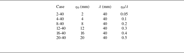
 η0
 λ

 a,b
 c
 d
 c
 d

 A0
 pvac
 pother

 a
 b,c
 d
 x
 t

 a
 b
 g(t)
 4
 ρR(t)
 ρL(t)
 g0
 ρR0
 ρL0

 μ

 a
 d
 e
 h
 a,e
 t=tL0
 b,f
 c,g
 d,h
 t=tR0
 ubbulk
 usbulk
 ubω
 usω
 p
 ω∗=(∂xuy−∂yux)/p0/ρ0
 ux
 uy
 x
 y
 p0
 ρ0
 −3
 i
 c
 Δui
 Δut
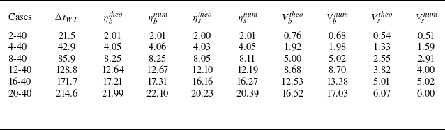
 ΔtWT
 ηb/stheo
 ηb/snum
 Vb/stheo
 Vb/snum
 μ
 −1
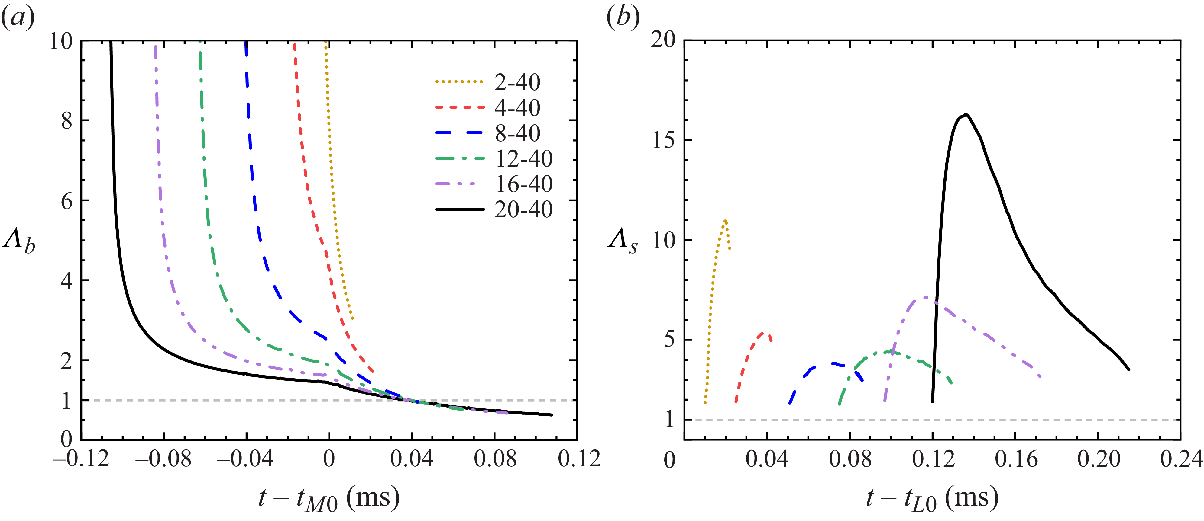
 Λb
 a
 Λs
 b

 a
 η1
 η2

 a
 b
 η0/λ
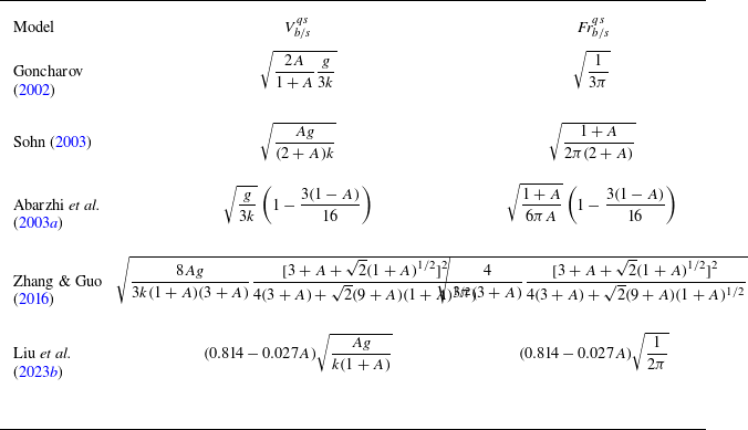
 Vb/sqs
 Frb/sqs
 A>0
 A<0

 a
 b
 c
 Vbi
 Vbs
 Vbc

 ω∗=(∂xuy−∂yux)/p0/ρ0
 a
 e
 f
 j
 t−tM0
 ηb−η0
 λ

 a
 c
 d
 f
 d
 e
 t−tM0
 k
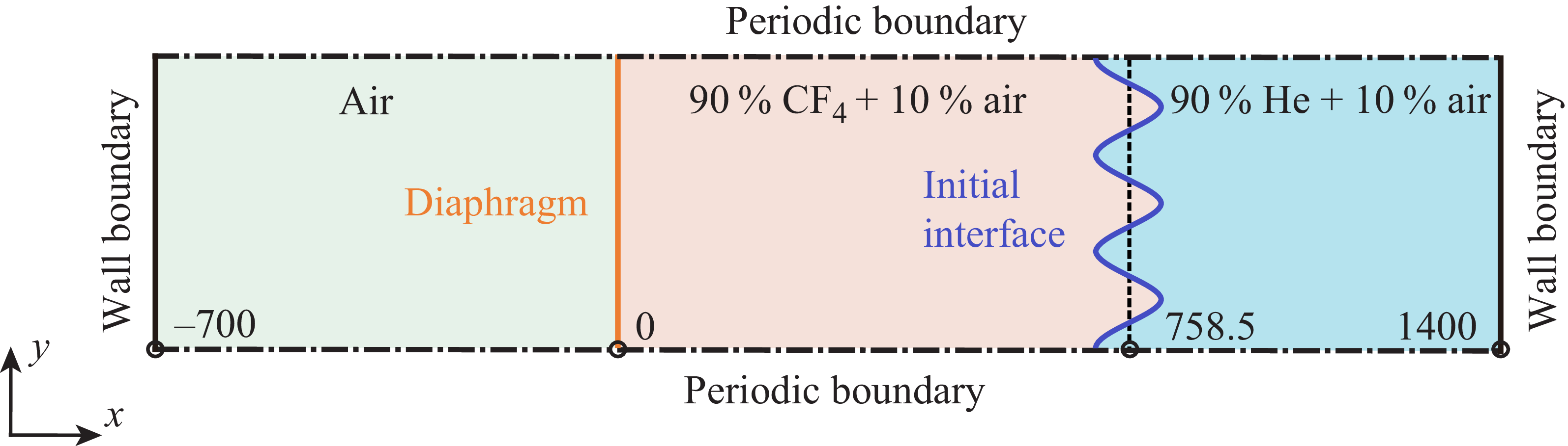

 a
 b
 c
 a,b


