1 Introduction
The complexity of a flow is often related to the concept of chaos (Ottino Reference Ottino1989, Reference Ottino1990; Wiggins & Ottino Reference Wiggins and Ottino2004; Loskutov Reference Loskutov2010; Aref et al. Reference Aref, Blake, Budišić, Cartwright, Clercx, Feudel, Golestanian, Gouillart, Guer and van Heijst2014). This has been studied from the perspective of dynamical systems and ergodic theory (Scott et al. Reference Scott, Redd, Kuznetsov, Mezić and Jones2009; Mathew & Mezić Reference Mathew and Mezić2011), introducing measures such as Lyapunov exponents and Kolmogorov–Sinai entropy, characterizing orbits and concepts such as Poincaré sections. A common feature of these measures is that they characterize flows infinitely propagated in time, in some sense representing the flow properties for large time scales. However, motivated by mixing problems, finite-time Lyapunov exponents have been also defined (Tang & Boozer Reference Tang and Boozer1996).
Poincaré sections have been also used (Ling Reference Ling1994; Funakoshi Reference Funakoshi2008; Jang & Funakoshi Reference Jang and Funakoshi2010; Xia et al. Reference Xia, Shu, Chew and Wang2010; Lucas & Kerswell Reference Lucas and Kerswell2014) to quantify chaotic mixing in cyclic systems, such as a periodic mixer or a helix-like pipe, after a number of loops. Poincaré sections can be used because the flow is considered cyclic, identifying the cross-sections after each cycle with the initial one.
Most methods to quantify fluid flow mixing have focused on measuring the homogenization of a scalar, representing a phase in a two-phase fluid or a physical property like temperature (Lin, Thiffeault & Doering Reference Lin, Thiffeault and Doering2011; Thiffeault Reference Thiffeault2012). Since the seminal work of Danckwerts (Reference Danckwerts1952) introducing the metrics scale and intensity of segregation (or variance of concentration), more complex metrics have been proposed, such as the Sobolev norm and the mix-norm (Mathew, Mezić & Petzold Reference Mathew, Mezić and Petzold2005) or the Shannon entropy (Camesasca, Kaufman & Manas-Zloczower Reference Camesasca, Kaufman and Manas-Zloczower2006) and Rényi entropy (Camesasca & Manas-Zloczower Reference Camesasca and Manas-Zloczower2009) of the scalar spatial distribution. In accordance with their purpose, all these metrics are dependent on the initial distribution of the studied scalar.
Brandani et al. (Reference Brandani, Schor, Macphee, Grubmüller, Zachariae and Marenduzzo2013) extended the idea of Camesasca et al. (Reference Camesasca, Kaufman and Manas-Zloczower2006) by using conditional entropy, but this was still applicable only to two-phase fluid flow mixing. It was applied to the design and evaluation of mixer devices (Domingues, Gaspar-Cunha & Covas Reference Domingues, Gaspar-Cunha and Covas2008). In contrast, Guida, Nienow & Barigou (Reference Guida, Nienow and Barigou2010) used conditional entropy to introduce a mixing measure of the flow itself, independent of any scalar distribution. They independently developed the same idea previously presented by Alemaskin et al. (Reference Alemaskin, Camesasca, Manas-Zloczower and Kaufman2004).
In most approaches, the fluid domain is discretized into a number of cells. This set of cells plays two different roles: defining the observation scale and acting as a convenient structure for computations. This double role can introduce some confusion. An explicit description of the observation scale and its relevance is found in Tucker & Peters (Reference Tucker and Peters2003), which introduced two mixing measures as functions of scale: sample standard deviation and sample max error, for two-phase fluids. Particles inside each cell are distributed with different proportions over several cells after some time. The distribution matrix (Kruijt et al. Reference Kruijt, Galaktionov, Anderson, Peters and Meijer2001) encodes this information and has been used as an ingredient in many works. In contrast, the multi-scale aggregate mix-norm proposed by Mathew et al. (Reference Mathew, Mezić and Petzold2005) assigns to each point centred balls of different radius. Each point contribution is then continuously integrated (no discretization), so that both roles are clearly separated.
A scalar-independent measure of chaotic mixing can be interpreted as a quantification of the complexity of the flow. Following this notion, we introduce in this paper the interlacing complexity index (ICI). It is independent of any scalar distribution and is valid for open systems with inlet and outlet flow regions. None of the existing flow complexity measures can be applied for these systems. The large-time-scale measures from dynamical systems theory are not applicable since the flow transport from the inlet to the outlet involves a finite time. The ICI quantifies the loss of spatial coherence owing to this flow transport. The inlet and outlet are surfaces on the control volume under study. Similarly to Poincaré sections, the observation locus is given by the crossing of the streamlines through these surfaces. However, they cannot be treated as Poincaré sections, since no identification between the inlet and the outlet is possible for general non-cyclic flows and control volumes.
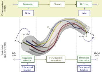
The ICI is inspired by communication theory (Shannon & Weaver Reference Shannon and Weaver1949), which deals with information flow as opposed to fluid flow. The basic scheme of a communication system involves a transmitter, a receiver and a communication channel. We can recognize parallel roles in those of, respectively, the inlet, the outlet and the flow transport between them. This analogy is illustrated in figure 1. The transmitted message is a position at the inlet, which is received as a corresponding position at the outlet, connected by a flow streamline and observed at a particular scale. In general, noise sources are also present in a communication system, producing some loss of information in the communication flow. Shanon’s mutual information (MI) measures the amount of information effectively communicated. Thus, for a perfectly laminar and parallel flow in a straight tube, the MI between input and output will be maximal. For more complex flows, generated by more intricate conditions or geometries, the ability to discriminate the outlet position by knowing the inlet position is decreased, reducing the corresponding MI.
Inlet–outlet open flow system analogy to a communication system. Each inlet point,
 $\boldsymbol{x}\in {\mathcal{S}}_{In}$
(input alphabet), is transmitted as a streamline,
 $\unicode[STIX]{x1D6FE}\in \unicode[STIX]{x1D6E4}_{{\mathcal{S}}}$
, propagated by the flow (ideal channel) up to the outlet. The streamline is received as a position
 $\boldsymbol{y}\in {\mathcal{S}}_{Out}$
(output alphabet) selected around the streamline crossing
 $\boldsymbol{x}_{Out}(\unicode[STIX]{x1D6FE})$
. The noise is modelled as a Gaussian point spread function, representing imprecision in the identification of points, with a standard deviation depending on the observation scale.

Hence, MI is a natural candidate to quantify fluid flow complexity in open flow systems as it is conceptually related to fluid transport from inlet to outlet. The ICI is defined as the normalization of this MI so that
 $\mathit{ICI}=0$
for the simplest parallel flow and
 $\mathit{ICI}\rightarrow 1$
for a very complex flow, producing practically unpredictable positions at the outlet from the positions at the inlet.
The ICI is not a single index but a function of the observation scale (
 $\mathit{ICI}_{s}$
). Thus, it can distinguish features appearing at different scales. The observation scale,
 $s$
, can be introduced by different protocols, for instance by a discretization or by a ball of specific radius as in Mathew et al. (Reference Mathew, Mezić and Petzold2005). Our implementation will follow this second approach but using Gaussian kernels instead of balls. To better understand the dependence of
 $\mathit{ICI}_{s}$
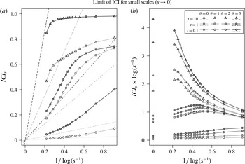
with the scale, we derive its limit for infinitesimal scales in appendix B.
At first glance, the global mixing measure proposed by Alemaskin et al. (Reference Alemaskin, Camesasca, Manas-Zloczower and Kaufman2004) and Guida et al. (Reference Guida, Nienow and Barigou2010) is the most similar to the ICI proposed here. It is independent of any scalar distribution and is defined as the average of Shannon’s conditional entropy. However, there are important differences. First, the definition of MI and conditional entropy are related but not equivalent and, hence, have different properties. The most notable difference is that conditional entropy, as entropy, is not well defined for continuous variables. The entropy of continuous variables, or differential entropy, does not coincide with the limit of the discrete entropy and is not invariant under parameter changes (Shannon Reference Shannon1948; Kolmogorov Reference Kolmogorov1956; Jaynes Reference Jaynes1968, Reference Jaynes2003). In contrast, the MI of continuous variables is the limit of the discrete case and is invariant to reparameterizations. Second, their mixing measure is based on the fluid particle propagation as a function of the time elapsed from the initial state and is observed in the full fluid domain. Thus, it is not applicable to open systems, i.e. those with specified inlets and outlets.
In order to properly define the ICI, the probability distribution of streamlines must be established. Herewith, we introduce the natural probability distribution of streamlines, which satisfies invariance with respect to the cross-section used to generate the streamlines. This probability density distribution is a relevant contribution in itself, which could be applied for visualization purposes or for any other statistics based on streamlines. The natural distribution of streamlines is valid for any steady flow and for any incompressible flow (steady or unsteady). For unsteady flows, a more natural alternative to streamlines are pathlines. Taking into account the temporal dimension, pathlines correspond to world-lines in the four-dimensional space–time. Thus, we also introduce the natural distribution of world-lines, with invariant properties for any flow satisfying the continuity equation. This involves the definition of the inlet and outlet as spatio-temporal hyper-surfaces. For unsteady incompressible flows, two versions of ICI are possible, considering either streamlines or world-lines. Although in that case world-lines reflects the actual flow transport, for some applications, considering the streamlines could be interesting. In particular, this allows a neat discrimination of flow features at different time instants.
The paper is organized as follows. Section 2 introduces the natural distribution of streamlines, demonstrating its invariant properties, together with a rigorous definition of the inlet and outlet. Section 3 defines the ICI, providing an intuitive interpretation. To illustrate and explore the properties of the proposed ICI, we apply it to several flow fields obtained either analytically or from numerical simulations. Section 4 describes the geometries and flows used for the numerical experiments in the subsequent sections, and the algorithm used for estimating the ICI using a finite sample of streamlines. In § 5, we evaluate the accuracy and precision of the estimated ICI for different algorithm settings, and the invariance with respect to the cross-section generating the streamlines. For the accuracy evaluation, we consider the analytical computation of the MI from a steady flow in a cylindrical straight tube, presented in appendix A. In § 6, we analyse the ICI of steady flows in two types of idealized geometries (non-coplanar double-bend tubes and rotating concentric cylinders) under different conditions. In § 7, the ICI of unsteady incompressible flows in more complex geometries (anatomically realistic vasculatures with aneurysms) is compared with subjective classifications of flow complexity and flow stability. In § 8, the world-lines version of ICI is obtained for unsteady compressible flows (two-dimensional (2-D) periodic cellular flows), and its behaviour for infinitesimal scales, derived in appendix B, is tested. Finally, § 9 presents the general conclusions.
2 Natural distribution of streamlines
2.1 Streamlines through a control volume
Let us consider any flow field
 $\boldsymbol{v}(\boldsymbol{x},t)$
defined in a spatio-temporal domain
 ${\mathcal{D}}\times {\mathcal{T}}$
, representing the local fluid speed at any point
 $\boldsymbol{x}\in {\mathcal{D}}$
at any time
 $t\in {\mathcal{T}}$
and with a fluid density
 $\unicode[STIX]{x1D70C}(\boldsymbol{x},t)$
. A streamline at a time
 $t$
is a line
 $\unicode[STIX]{x1D6FE}$
whose tangent vector is parallel to the flow field at that time at all points along the line. Parameterized with a pseudo-time
 $\unicode[STIX]{x1D70F}$
,
 $$\begin{eqnarray}\displaystyle \unicode[STIX]{x1D738}:I\rightarrow {\mathcal{D}};\quad \unicode[STIX]{x1D70F}\mapsto \unicode[STIX]{x1D738}(\unicode[STIX]{x1D70F}),\quad \text{such that}~\frac{\text{d}}{\text{d}\unicode[STIX]{x1D70F}}\unicode[STIX]{x1D738}(\unicode[STIX]{x1D70F})=\boldsymbol{v}(\unicode[STIX]{x1D738}(\unicode[STIX]{x1D70F}),t), & & \displaystyle\end{eqnarray}$$
where we consider the interval,
 $I\subset \mathbb{R}$
, that maximally extends the streamline in
 ${\mathcal{D}}$
. We will denote by
 $\unicode[STIX]{x1D6FE}$
(no boldface) the streamline trajectory regardless of its parameterization. The congruence of streamlines,
 $\unicode[STIX]{x1D6E4}(t)$
, is the set of all streamlines in
 ${\mathcal{D}}$
at any given instant
 $t$
. For simplicity, let us fix a time
 $t$
, and assume it in the notation, as for
 $\boldsymbol{v}(\boldsymbol{x}):=\boldsymbol{v}(\boldsymbol{x},t)$
and
 $\unicode[STIX]{x1D6E4}:=\unicode[STIX]{x1D6E4}(t)$
.
Let us consider a control volume
 ${\mathcal{D}}_{{\mathcal{S}}}\subset {\mathcal{D}}$
enclosed by a control surface
 ${\mathcal{S}}$
, with a strictly positive scalar field,
 $\unicode[STIX]{x1D6FC}(\boldsymbol{x})>0~\forall x\in {\mathcal{D}}$
, defining a current
 $\boldsymbol{j}(\boldsymbol{x})=\unicode[STIX]{x1D6FC}(\boldsymbol{x})\,\boldsymbol{v}(\boldsymbol{x})$
.
Definition 1. At any point on the control surface,
 $\boldsymbol{x}\in {\mathcal{S}}$
, the
 $\boldsymbol{j}$
-flux density (flow rate per unit area) through the surface
 ${\mathcal{S}}$
will be
 $$\begin{eqnarray}\unicode[STIX]{x1D711}_{\boldsymbol{j}}^{{\mathcal{S}}}(\boldsymbol{x}):=\boldsymbol{j}(\boldsymbol{x})\boldsymbol{\cdot }\hat{\boldsymbol{n}}_{{\mathcal{S}}}(\boldsymbol{x}),\end{eqnarray}$$
where
 $\hat{\boldsymbol{n}}_{{\mathcal{S}}}(\boldsymbol{x})$
is the unit normal vector to
 ${\mathcal{S}}$
at the point
 $\boldsymbol{x}$
, pointing outwards. For any subregion
 ${\mathcal{A}}\subset {\mathcal{S}}$
, the corresponding flux will be the surface integral on the subregion,
 $$\begin{eqnarray}\unicode[STIX]{x1D6F7}_{\boldsymbol{j}}({\mathcal{A}}):=\int _{{\mathcal{A}}}\unicode[STIX]{x1D711}_{\boldsymbol{j}}^{{\mathcal{S}}}(\boldsymbol{x})\,\text{d}S=\int _{{\mathcal{A}}}\boldsymbol{j}(\boldsymbol{x})\boldsymbol{\cdot }\mathbf{d}\boldsymbol{S},\end{eqnarray}$$
where
 $\text{d}S$
and
 $\mathbf{d}\boldsymbol{S}$
denote the scalar and vector surface element, respectively.
In particular, we will consider the volume flow rate,
 $\unicode[STIX]{x1D711}_{\boldsymbol{v}}^{{\mathcal{S}}}(\boldsymbol{x})$
, corresponding to
 $\unicode[STIX]{x1D6FC}(\boldsymbol{x})=1$
, and the mass flow rate generated by
 $\boldsymbol{j}(\boldsymbol{x})=\unicode[STIX]{x1D70C}(\boldsymbol{x})\,\boldsymbol{v}(\boldsymbol{x})$
.
The flux density will be negative at entry points and positive at exit points. Thus, the control surface
 ${\mathcal{S}}$
can be accordingly split into two regions:
 $$\begin{eqnarray}\displaystyle \overline{{\mathcal{S}}}_{In}:=\{\boldsymbol{x}\in {\mathcal{S}}\,|\,\unicode[STIX]{x1D711}_{\boldsymbol{v}}^{{\mathcal{S}}}(\boldsymbol{x})<0\}\quad \text{and}\quad \overline{{\mathcal{S}}}_{Out}:=\{\boldsymbol{x}\in {\mathcal{S}}\,|\,\unicode[STIX]{x1D711}_{\boldsymbol{v}}^{{\mathcal{S}}}(\boldsymbol{x})>0\}. & & \displaystyle\end{eqnarray}$$
There is indeed a third region,
 $\overline{{\mathcal{S}}}_{0}:=\{\boldsymbol{x}\in {\mathcal{S}}\,|\,\unicode[STIX]{x1D711}_{\boldsymbol{v}}^{{\mathcal{S}}}(\boldsymbol{x})=0\}$
, where the streamlines are tangent to the surface. In particular, if
 ${\mathcal{S}}$
includes rigid walls delimiting the fluid, they will be included in
 $\overline{{\mathcal{S}}}_{0}$
.
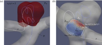
Example of recirculation at the entrance of a control volume
 ${\mathcal{D}}_{{\mathcal{S}}}$
, represented in red (a). One streamline is shown with recirculation number
 $r_{{\mathcal{S}}}(\unicode[STIX]{x1D6FE})=2$
. The two inward points are represented in white and the two outward points in black (b). The entrance is divided into two surfaces,
 $\overline{{\mathcal{S}}}_{In}$
and
 $\overline{{\mathcal{S}}}_{Out}$
, according to the flux sign.

A streamline
 $\unicode[STIX]{x1D6FE}\in \unicode[STIX]{x1D6E4}$
can miss
 ${\mathcal{D}}_{{\mathcal{S}}}$
, enter once or repeatedly enter and exit
 ${\mathcal{D}}_{{\mathcal{S}}}$
. Let us denote the number of times that the streamline enters and exits
 ${\mathcal{D}}_{{\mathcal{S}}}$
by, respectively,
 $$\begin{eqnarray}\displaystyle r_{{\mathcal{S}}}^{In}(\unicode[STIX]{x1D6FE}):=\text{Card}(\unicode[STIX]{x1D6FE}\cap \overline{{\mathcal{S}}}_{In})\quad \text{and}\quad r_{{\mathcal{S}}}^{Out}(\unicode[STIX]{x1D6FE}):=\text{Card}(\unicode[STIX]{x1D6FE}\cap \overline{{\mathcal{S}}}_{Out}). & & \displaystyle\end{eqnarray}$$
The
 $r_{{\mathcal{S}}}^{In}(\unicode[STIX]{x1D6FE})$
points in the intersection
 $\unicode[STIX]{x1D6FE}\cap \overline{{\mathcal{S}}}_{In}$
can be sorted according to the crossing order:
 $\boldsymbol{x}_{In,i}(\unicode[STIX]{x1D6FE})$
, for
 $i=1,2,\ldots ,r_{{\mathcal{S}}}^{In}(\unicode[STIX]{x1D6FE})$
. Analogously for the
 $r_{{\mathcal{S}}}^{Out}(\unicode[STIX]{x1D6FE})$
points in
 $\unicode[STIX]{x1D6FE}\cap \overline{{\mathcal{S}}}_{Out}$
.
Assuming that there is no sink or source inside the control volume, each streamline will in general exit as many times as it enters. Strictly speaking, some exceptional cases can appear, involving equilibrium points or cycles. However, under reasonable assumptions, they would represent a zero-measure set of streamlines, and will be discarded in the following definition.
Definition 2. The congruence of
 ${\mathcal{S}}$
-crossing streamlines will be the set
 $$\begin{eqnarray}\displaystyle \unicode[STIX]{x1D6E4}_{{\mathcal{S}}}:=\{\unicode[STIX]{x1D6FE}\in \unicode[STIX]{x1D6E4}\mid r_{{\mathcal{S}}}^{In}(\unicode[STIX]{x1D6FE})=r_{{\mathcal{S}}}^{Out}(\unicode[STIX]{x1D6FE})>0\}. & & \displaystyle\end{eqnarray}$$
The number of times that a streamline
 $\unicode[STIX]{x1D6FE}\in \unicode[STIX]{x1D6E4}_{{\mathcal{S}}}$
enters the control volume
 ${\mathcal{D}}_{{\mathcal{S}}}$
will be called its recirculation number, and will be denoted by
 $r_{{\mathcal{S}}}(\unicode[STIX]{x1D6FE})$
.
Figure 2 illustrates these concepts.
Definition 3. For each streamline
 $\unicode[STIX]{x1D6FE}\in \unicode[STIX]{x1D6E4}_{{\mathcal{S}}}$
, the first inwards crossing point will be called its inlet point,
 $\boldsymbol{x}_{In}(\unicode[STIX]{x1D6FE}):=\boldsymbol{x}_{In,1}(\unicode[STIX]{x1D6FE})$
, and the last outwards crossing point its outlet point,
 $\boldsymbol{x}_{Out}(\unicode[STIX]{x1D6FE}):=\boldsymbol{x}_{Out,r_{{\mathcal{S}}}(\unicode[STIX]{x1D6FE})}(\unicode[STIX]{x1D6FE})$
. The sets containing all inlet and outlet points,
 $$\begin{eqnarray}{\mathcal{S}}_{In}:=\{\boldsymbol{x}_{In}(\unicode[STIX]{x1D6FE})\mid \unicode[STIX]{x1D6FE}\in \unicode[STIX]{x1D6E4}_{{\mathcal{S}}}\}\quad \text{and}\quad {\mathcal{S}}_{Out}:=\{\boldsymbol{x}_{Out}(\unicode[STIX]{x1D6FE})\mid \unicode[STIX]{x1D6FE}\in \unicode[STIX]{x1D6E4}_{{\mathcal{S}}}\},\end{eqnarray}$$
will be called inlet and outlet, respectively.
This definition guarantees that there exist bijective mappings between inlet, outlet and the congruence of streamlines
 $\unicode[STIX]{x1D6E4}_{{\mathcal{S}}}$
. Notice that, although the union of the streamlines fills the three-dimensional domain, the congruence of streamlines is a two-dimensional set. Since
 $\boldsymbol{x}_{In}:\unicode[STIX]{x1D6E4}_{{\mathcal{S}}}\rightarrow {\mathcal{S}}_{In}$
is a bijection,
 $\boldsymbol{x}_{In}(\unicode[STIX]{x1D6FE})$
can be used as a parameterization of
 $\unicode[STIX]{x1D6FE}$
. Analogously,
 $\boldsymbol{x}_{Out}(\unicode[STIX]{x1D6FE})$
gives an alternative parameterization.
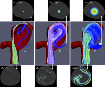
Three examples of streamlines bundles generated by their crossing at the outlet (top) defined as a circle around a point with three different radii. The crossing at the inlet (bottom) is very elongated and the complexity of the obtained pattern depends on the scale considered.

2.2 Probability distribution of streamlines
The computation of any statistical quantity from a streamline distribution requires the definition of a probability density of streamlines. A natural selection is to make the probability density proportional to the local flux, thereby considering denser presence of streamlines where the flow rate is larger.
Definition 4. Parameterizing streamlines
 $\unicode[STIX]{x1D6FE}\in \unicode[STIX]{x1D6E4}_{{\mathcal{S}}}$
by their crossing at the inlet
 $\boldsymbol{x}=\boldsymbol{x}_{In}(\unicode[STIX]{x1D6FE})$
, the (
 $\boldsymbol{j}$
-)natural distribution of streamlines will be given by the surface probability density
 $$\begin{eqnarray}p_{In}(\boldsymbol{x})=\frac{\unicode[STIX]{x1D711}_{\boldsymbol{j}}^{{\mathcal{S}}}(\boldsymbol{x})}{\unicode[STIX]{x1D6F7}_{\boldsymbol{j}}({\mathcal{S}}_{In})}\quad \forall \boldsymbol{x}\in {\mathcal{S}}_{In}.\end{eqnarray}$$
Any bundle of streamlines,
 $\unicode[STIX]{x1D6F6}\subset \unicode[STIX]{x1D6E4}_{{\mathcal{S}}}$
, will define a subregion of the inlet by its crossing,
 ${\mathcal{A}}_{In}(\unicode[STIX]{x1D6F6})=\unicode[STIX]{x1D6F6}\cap {\mathcal{S}}_{In}$
, and a subregion of the outlet,
 ${\mathcal{A}}_{Out}(\unicode[STIX]{x1D6F6})=\unicode[STIX]{x1D6F6}\cap {\mathcal{S}}_{Out}$
(see figure 3). Accordingly, the probability of a streamline bundle
 $\unicode[STIX]{x1D6F6}\subset \unicode[STIX]{x1D6E4}_{{\mathcal{S}}}$
will be
 $$\begin{eqnarray}P_{In}(\unicode[STIX]{x1D6F6})=\int _{{\mathcal{A}}_{In}(\unicode[STIX]{x1D6F6})}p_{In}(\boldsymbol{x})\,\text{d}S=\frac{\unicode[STIX]{x1D6F7}_{\boldsymbol{j}}({\mathcal{A}}_{In}(\unicode[STIX]{x1D6F6}))}{\unicode[STIX]{x1D6F7}_{\boldsymbol{j}}({\mathcal{S}}_{In})}.\end{eqnarray}$$
Analogously,
 $p_{Out}(\boldsymbol{x})$
and
 $P_{Out}(\unicode[STIX]{x1D6F6})$
are defined by their crossing at the outlet. Indeed, for any surface intersecting once every streamline in
 $\unicode[STIX]{x1D6E4}_{{\mathcal{S}}}$
, we could define the corresponding probability density.
Strictly speaking, we are considering here volumetric probabilities instead of probability densities, in the sense discussed in Tarantola (Reference Tarantola2005) and Tarantola & Mosegaard (Reference Tarantola and Mosegaard2007), since they are defined with respect to the surface element,
 $\text{d}S$
, and independently of any coordinate system.
Lemma 1. For any divergence-free current,
 $\unicode[STIX]{x1D735}\boldsymbol{\cdot }\boldsymbol{j}(\boldsymbol{x})=0$
, the flux corresponding to any bundle of streamlines
 $\unicode[STIX]{x1D6F6}\subset \unicode[STIX]{x1D6E4}_{{\mathcal{S}}}$
is constant along the streamlines (invariant with respect to the cross-section considered):
 $$\begin{eqnarray}\displaystyle \unicode[STIX]{x1D6F7}_{\boldsymbol{j}}({\mathcal{A}}_{In}(\unicode[STIX]{x1D6F6}))=\unicode[STIX]{x1D6F7}_{\boldsymbol{j}}({\mathcal{A}}_{Out}(\unicode[STIX]{x1D6F6})), & & \displaystyle\end{eqnarray}$$
and its natural probability distribution of streamlines is invariant with respect to the cross-section used to parameterize the streamlines:
 $$\begin{eqnarray}\displaystyle P_{In}(\unicode[STIX]{x1D6F6})=P_{Out}(\unicode[STIX]{x1D6F6}). & & \displaystyle\end{eqnarray}$$
Thus, we can simply denote it as
 $P(\unicode[STIX]{x1D6F6})$
.
Proof. It follows from the divergence theorem applied to small streamtubes.◻
Proposition 1 (Incompressible flows).
For an incompressible flow, the
 $\boldsymbol{v}$
-natural probability distribution is invariant with respect to the cross-section used to parameterize the streamlines.
Proof. An incompressible flow is characterized by
 $\unicode[STIX]{x1D735}\boldsymbol{\cdot }\boldsymbol{v}=0$
.◻
Proposition 2 (Steady flows).
For a steady flow, the
 $\boldsymbol{j}$
-natural probability distribution, for the mass current
 $\boldsymbol{j}=\unicode[STIX]{x1D70C}\,\boldsymbol{v}$
, is invariant with respect to the cross-section used to parameterize the streamlines.
Proof. For a steady flow, the density at each point is temporally constant,
 $\unicode[STIX]{x2202}\unicode[STIX]{x1D70C}/\unicode[STIX]{x2202}t=0$
. Then, the continuity equation implies
 $$\begin{eqnarray}\displaystyle \frac{\unicode[STIX]{x2202}}{\unicode[STIX]{x2202}t}\unicode[STIX]{x1D70C}+\unicode[STIX]{x1D735}\boldsymbol{\cdot }(\unicode[STIX]{x1D70C}\,\boldsymbol{v})=\unicode[STIX]{x1D735}\boldsymbol{\cdot }\boldsymbol{j}=0. & & \displaystyle\end{eqnarray}$$
◻
Observe that for a homogeneous incompressible flow, the probability distribution generated by the mass flux coincides with the probability distribution generated by the volume flux.
Proposition 3 (General flow with density propagated by (pseudo) advection).
The propagation by advection along any instantaneous flow
 $\boldsymbol{v}(\boldsymbol{x})=\boldsymbol{v}(\boldsymbol{x},t_{0})$
, of any density
 $\unicode[STIX]{x1D6FC}(x)$
defined at the inlet or outlet, provides a conserved current,
 $\boldsymbol{j}=\unicode[STIX]{x1D6FC}\boldsymbol{v}$
, with invariant
 $\boldsymbol{j}$
-natural probability density of streamlines.
Proof. Let
 $\unicode[STIX]{x1D70F}(\boldsymbol{x})$
denote the function providing the pseudo-time parameter,
 $\unicode[STIX]{x1D70F}$
, in the corresponding streamline
 $\unicode[STIX]{x1D6FE}$
, so that
 $\boldsymbol{x}=\unicode[STIX]{x1D738}(\unicode[STIX]{x1D70F})$
. Let us consider a density
 $c(\boldsymbol{x},\unicode[STIX]{x1D70F})$
generated by advection along the flow
 $\boldsymbol{v}(\boldsymbol{x})$
:
 $$\begin{eqnarray}\frac{\unicode[STIX]{x2202}c(\boldsymbol{x},\unicode[STIX]{x1D70F})}{\unicode[STIX]{x2202}\unicode[STIX]{x1D70F}}+\unicode[STIX]{x1D735}\boldsymbol{\cdot }(c(\boldsymbol{x},\unicode[STIX]{x1D70F})\,\boldsymbol{v}(\boldsymbol{x}))=0,\quad \text{with}~c(\boldsymbol{x}_{In},\unicode[STIX]{x1D70F}_{In})=\unicode[STIX]{x1D6FC}(\boldsymbol{x}_{In})~\forall \unicode[STIX]{x1D6FE}\in \unicode[STIX]{x1D6E4}_{{\mathcal{S}}}.\end{eqnarray}$$
Then, the density
 $\unicode[STIX]{x1D6FC}(\boldsymbol{x}):=c(\boldsymbol{x},\unicode[STIX]{x1D70F}(\boldsymbol{x}))$
provides a conserved current,
 $\boldsymbol{j}(\boldsymbol{x})=\unicode[STIX]{x1D6FC}(\boldsymbol{x})\,\boldsymbol{v}(\boldsymbol{x})$
:
 $$\begin{eqnarray}\displaystyle \unicode[STIX]{x1D735}\boldsymbol{\cdot }\boldsymbol{j}(\boldsymbol{x})=\unicode[STIX]{x1D735}\boldsymbol{\cdot }(c(\boldsymbol{x},\unicode[STIX]{x1D70F})\,\boldsymbol{v}(\boldsymbol{x}))|_{\unicode[STIX]{x1D70F}=\unicode[STIX]{x1D70F}(\boldsymbol{x})}+\left.\frac{\unicode[STIX]{x2202}c(\boldsymbol{x},\unicode[STIX]{x1D70F})}{\unicode[STIX]{x2202}\unicode[STIX]{x1D70F}}\right|_{\unicode[STIX]{x1D70F}=\unicode[STIX]{x1D70F}(\boldsymbol{x})}\boldsymbol{v}(\boldsymbol{x})\boldsymbol{\cdot }\unicode[STIX]{x1D735}\unicode[STIX]{x1D70F}(\boldsymbol{x})=0, & & \displaystyle\end{eqnarray}$$
where we have used (2.13) and the property
 $\boldsymbol{v}(\boldsymbol{x})\boldsymbol{\cdot }\unicode[STIX]{x1D735}\unicode[STIX]{x1D70F}(\boldsymbol{x})=1$
.◻
In these cases, the natural probability density is a property of the streamlines, independently of the cross-section considered. We will symbolically denote it as
 $p(\unicode[STIX]{x1D6FE})$
. Note that the naive homogenous distribution would be cross-section dependent. In general, it would be inhomogeneous for any other cross-section.
2.3 Source of non-invariance of the natural distribution of streamlines
Whenever the current
 $\boldsymbol{j}=\unicode[STIX]{x1D6FC}\boldsymbol{v}$
is not divergence free,
 $\unicode[STIX]{x1D735}\boldsymbol{\cdot }\boldsymbol{j}\neq 0$
, the corresponding flux cannot be guaranteed to be conserved, and the probability distribution of streamlines will not be invariant. In our experiments, we will consider homogeneous incompressible flows, which should satisfy
 $\unicode[STIX]{x1D735}\boldsymbol{\cdot }\boldsymbol{j}=0$
. However, when a flow is obtained by computer flow simulation, numerical inaccuracies might arise, which justifies studying their influence in the probability distribution invariance.
Lemma 2. Given a streamline bundle,
 $\text{d}\unicode[STIX]{x1D6F6}$
, of infinitesimal cross-section (streamtube) around a streamline
 $\unicode[STIX]{x1D6FE}\in \unicode[STIX]{x1D6E4}_{{\mathcal{S}}}$
, propagating from inlet to outlet:
 $$\begin{eqnarray}\displaystyle \unicode[STIX]{x1D738}(\unicode[STIX]{x1D70F}_{In})=\boldsymbol{x}_{In}\in {\mathcal{A}}_{In}(\text{d}\unicode[STIX]{x1D6F6})\subset {\mathcal{S}}_{In}\quad \mathit{and}\quad \unicode[STIX]{x1D738}(\unicode[STIX]{x1D70F}_{Out})=\boldsymbol{x}_{Out}\in {\mathcal{A}}_{Out}(\text{d}\unicode[STIX]{x1D6F6})\subset {\mathcal{S}}_{Out}, & & \displaystyle\end{eqnarray}$$
the fluxes of the current
 $\boldsymbol{j}=\unicode[STIX]{x1D6FC}\boldsymbol{v}$
at the inlet and outlet are related by
 $$\begin{eqnarray}\displaystyle \unicode[STIX]{x1D6F7}_{\boldsymbol{j}}({\mathcal{A}}_{Out}(\text{d}\unicode[STIX]{x1D6F6}))=\text{e}^{\unicode[STIX]{x1D709}(\unicode[STIX]{x1D6FE})}\,\unicode[STIX]{x1D6F7}_{\boldsymbol{j}}({\mathcal{A}}_{In}(\text{d}\unicode[STIX]{x1D6F6})), & & \displaystyle\end{eqnarray}$$
where the factor exponent is given by the temporal integral of the flow divergence along the streamline,
 $$\begin{eqnarray}\displaystyle \unicode[STIX]{x1D709}(\unicode[STIX]{x1D6FE}):=\int _{\unicode[STIX]{x1D70F}_{In}}^{\unicode[STIX]{x1D70F}_{Out}}\frac{1}{\unicode[STIX]{x1D6FC}(\unicode[STIX]{x1D738}(\unicode[STIX]{x1D70F}))}\unicode[STIX]{x1D735}\boldsymbol{\cdot }\boldsymbol{j}(\unicode[STIX]{x1D738}(\unicode[STIX]{x1D70F}))\,\text{d}\unicode[STIX]{x1D70F}. & & \displaystyle\end{eqnarray}$$
For divergence-free currents,
 $\unicode[STIX]{x1D709}(\unicode[STIX]{x1D6FE})=0$
, so that the flux is conserved. Thus, the factor exponent
 $\unicode[STIX]{x1D709}(\unicode[STIX]{x1D6FE})$
is the source of non-invariance of the corresponding natural distribution of streamlines. For incompressible flows (
 $\boldsymbol{j}=\boldsymbol{v}$
), the integral simplifies to
 $$\begin{eqnarray}\unicode[STIX]{x1D709}(\unicode[STIX]{x1D6FE})=\int _{\unicode[STIX]{x1D70F}_{In}}^{\unicode[STIX]{x1D70F}_{Out}}\unicode[STIX]{x1D735}\boldsymbol{\cdot }\boldsymbol{v}(\unicode[STIX]{x1D738}(\unicode[STIX]{x1D70F}))\,\text{d}\unicode[STIX]{x1D70F}.\end{eqnarray}$$
Proof. Let us consider any density
 $\unicode[STIX]{x1D6FC}^{\prime }(\boldsymbol{x})$
generated by advection along
 $\boldsymbol{v}(\boldsymbol{x})$
, as defined in proposition 3. Then, the current
 $\boldsymbol{j}^{\prime }=\unicode[STIX]{x1D6FC}^{\prime }\boldsymbol{v}$
provides a conserved flux. Since the new current is proportional to the original one,
 $\boldsymbol{j}^{\prime }=\unicode[STIX]{x1D6FD}\boldsymbol{j}$
, where
 $\unicode[STIX]{x1D6FD}=\unicode[STIX]{x1D6FC}^{\prime }/\unicode[STIX]{x1D6FC}$
, their fluxes are also proportional. Thus, the conservation of
 $\boldsymbol{j}^{\prime }$
provides the relationship
 $$\begin{eqnarray}\unicode[STIX]{x1D6F7}_{\boldsymbol{j}}({\mathcal{A}}_{Out}(\text{d}\unicode[STIX]{x1D6F6}))=\frac{\unicode[STIX]{x1D6FD}(\boldsymbol{x}_{In})}{\unicode[STIX]{x1D6FD}(\boldsymbol{x}_{Out})}\unicode[STIX]{x1D6F7}_{\boldsymbol{j}}({\mathcal{A}}_{In}(\text{d}\unicode[STIX]{x1D6F6})).\end{eqnarray}$$
Besides,
 $$\begin{eqnarray}\unicode[STIX]{x1D735}\boldsymbol{\cdot }\boldsymbol{j}^{\prime }=0\quad \Rightarrow \quad \boldsymbol{j}\boldsymbol{\cdot }\unicode[STIX]{x1D735}\unicode[STIX]{x1D6FD}+\unicode[STIX]{x1D6FD}\,\unicode[STIX]{x1D735}\boldsymbol{\cdot }\boldsymbol{j}=0\quad \Rightarrow \quad \boldsymbol{j}\boldsymbol{\cdot }\unicode[STIX]{x1D735}\log (\unicode[STIX]{x1D6FD})=-\unicode[STIX]{x1D735}\boldsymbol{\cdot }\boldsymbol{j}.\end{eqnarray}$$
For any point in the streamline,
 $\boldsymbol{x}=\unicode[STIX]{x1D738}(\unicode[STIX]{x1D70F})$
, the directional derivative along
 $\boldsymbol{j}=\unicode[STIX]{x1D6FC}\boldsymbol{v}$
can be expressed in terms of the time derivative:
 $$\begin{eqnarray}\boldsymbol{j}\boldsymbol{\cdot }\unicode[STIX]{x1D735}\log (\unicode[STIX]{x1D6FD}(\boldsymbol{x}))=\unicode[STIX]{x1D6FC}(\boldsymbol{x})\frac{\text{d}}{\text{d}\unicode[STIX]{x1D70F}}\log (\unicode[STIX]{x1D6FD}(\unicode[STIX]{x1D738}(\unicode[STIX]{x1D70F}))).\end{eqnarray}$$
Substituting (2.21) into (2.20) and integrating along the streamline from inlet to outlet:
 $$\begin{eqnarray}\displaystyle \log \frac{\unicode[STIX]{x1D6FD}(\boldsymbol{x}_{In})}{\unicode[STIX]{x1D6FD}(\boldsymbol{x}_{Out})}=\int _{\unicode[STIX]{x1D70F}_{In}}^{\unicode[STIX]{x1D70F}_{Out}}\frac{1}{\unicode[STIX]{x1D6FC}(\unicode[STIX]{x1D738}(\unicode[STIX]{x1D70F}))}\,\unicode[STIX]{x1D735}\boldsymbol{\cdot }\boldsymbol{j}(\unicode[STIX]{x1D738}(\unicode[STIX]{x1D70F}))\,\text{d}\unicode[STIX]{x1D70F}=\unicode[STIX]{x1D709}(\unicode[STIX]{x1D6FE}). & & \displaystyle\end{eqnarray}$$
◻
2.4 Natural probability distribution of world-lines
For unsteady flows, particle trajectories (pathlines) are generally different from streamlines. Pathlines are normally understood as the trajectories in the space, considering the temporal dimension only as the pathline parameter,
 $$\begin{eqnarray}\displaystyle \unicode[STIX]{x1D738}:I\rightarrow {\mathcal{D}};\quad t\mapsto \unicode[STIX]{x1D738}(t),\quad \text{such that}~\frac{\text{d}}{\text{d }t}\unicode[STIX]{x1D738}(t)=\boldsymbol{v}(\unicode[STIX]{x1D738}(t),t). & & \displaystyle\end{eqnarray}$$
However, particle trajectories can be understood as streamlines in the 4-D Galilean space–time, called world-lines. Let us consider the 4-D Cartesian coordinates and the 4-D velocity field
 $$\begin{eqnarray}\displaystyle x^{\unicode[STIX]{x1D707}}=(x^{0},x^{1},x^{2},x^{3})=(t,\boldsymbol{x})\quad \text{and}\quad v^{\unicode[STIX]{x1D707}}(\{x^{\unicode[STIX]{x1D708}}\})=(1,\boldsymbol{v}(\boldsymbol{x},t)), & & \displaystyle\end{eqnarray}$$
where Greek indices range from 0 to 3. This notation is partially borrowed from special relativity physics, but it is compatible with Galilean relativity and Newtonian mechanics.
World-lines represent the particle trajectories in the space–time and are computed as the streamlines of this 4-D flow:
 $$\begin{eqnarray}\displaystyle \unicode[STIX]{x1D6FE}^{\unicode[STIX]{x1D707}}:I\rightarrow {\mathcal{T}}\times {\mathcal{D}};\quad \unicode[STIX]{x1D70F}\mapsto \unicode[STIX]{x1D6FE}^{\unicode[STIX]{x1D707}}(\unicode[STIX]{x1D70F}),\quad \text{such that}~\frac{\text{d}}{\text{d}\unicode[STIX]{x1D70F}}\,\unicode[STIX]{x1D6FE}^{\unicode[STIX]{x1D707}}(\unicode[STIX]{x1D70F})=v^{\unicode[STIX]{x1D707}}(\{\unicode[STIX]{x1D6FE}^{\unicode[STIX]{x1D707}}(\unicode[STIX]{x1D70F})\}), & & \displaystyle\end{eqnarray}$$
which, together with the initial condition
 $\unicode[STIX]{x1D6FE}^{0}(\unicode[STIX]{x1D70F}_{0})=\unicode[STIX]{x1D70F}_{0}$
, is equivalent to the pathline equation
 $$\begin{eqnarray}\displaystyle \unicode[STIX]{x1D6FE}^{0}(\unicode[STIX]{x1D70F})=\unicode[STIX]{x1D70F}\quad \text{and}\quad \frac{\text{d}}{\text{d}\unicode[STIX]{x1D70F}}\unicode[STIX]{x1D738}(\unicode[STIX]{x1D70F})=\boldsymbol{v}(\unicode[STIX]{x1D738}(\unicode[STIX]{x1D70F}),\unicode[STIX]{x1D70F}). & & \displaystyle\end{eqnarray}$$
The 4-D nabla operator is denoted
 $$\begin{eqnarray}\displaystyle \unicode[STIX]{x1D6FB}_{\unicode[STIX]{x1D707}}=\left(\frac{\unicode[STIX]{x2202}}{\unicode[STIX]{x2202}x^{0}},\frac{\unicode[STIX]{x2202}}{\unicode[STIX]{x2202}x^{1}},\frac{\unicode[STIX]{x2202}}{\unicode[STIX]{x2202}x^{2}},\frac{\unicode[STIX]{x2202}}{\unicode[STIX]{x2202}x^{3}}\right)=\left(\frac{\unicode[STIX]{x2202}}{\unicode[STIX]{x2202}t},\unicode[STIX]{x1D735}\right). & & \displaystyle\end{eqnarray}$$
The mass flow current is then
 $j^{\unicode[STIX]{x1D707}}:=\unicode[STIX]{x1D70C}v^{\unicode[STIX]{x1D707}}$
, for which the continuity equation is simply written in terms of the 4-D divergence:
 $$\begin{eqnarray}\unicode[STIX]{x1D6FB}_{\unicode[STIX]{x1D707}}j^{\unicode[STIX]{x1D707}}=\frac{\unicode[STIX]{x2202}}{\unicode[STIX]{x2202}t}\,\unicode[STIX]{x1D70C}+\unicode[STIX]{x1D735}\boldsymbol{\cdot }(\unicode[STIX]{x1D70C}\boldsymbol{v})=0.\end{eqnarray}$$
Hence, all definitions and properties described above for streamlines of incompressible flows are valid for world-lines of any (mass preserving) flow. Thus the natural distribution of world-lines appears as follows. Considering a 4-D control hyper-volume, its boundary would be a 3-D hyper-surface, from which the corresponding inlet and outlet hyper-surfaces can be defined according to the flux density derived from
 $j^{\unicode[STIX]{x1D707}}$
. This flux defines then a probability density invariant to the cross-sectional hyper-surface.
3 Interlacing complexity index based on mutual information
If a small area,
 ${\mathcal{A}}_{In}$
, is singled out at the inlet, the corresponding bundle of streamlines,
 $\unicode[STIX]{x1D6E4}$
, will determine the corresponding outlet area,
 ${\mathcal{A}}_{Out}$
. Depending on the complexity of the flow from inlet to outlet, a simple and compact input area can correspond to a complex and elongated output (see figure 3). We propose to measure the flow complexity by an index derived from Shanon’s MI between corresponding inlet position,
 $\boldsymbol{x}_{In}$
, and outlet position,
 $\boldsymbol{x}_{Out}$
, of the streamlines,
 $\unicode[STIX]{x1D6FE}\in \unicode[STIX]{x1D6E4}_{{\mathcal{S}}}$
.
The MI of two variables of interest,
 $\!\boldsymbol{X}_{\!In}$
and
 $\!\boldsymbol{X}_{\!Out}$
, is computed from the corresponding joint probability density,
 $p(\boldsymbol{x}_{In},\boldsymbol{x}_{Out})$
:
 $$\begin{eqnarray}I(\boldsymbol{X}_{\!In},\boldsymbol{X}_{\!Out})=\int _{{\mathcal{S}}_{In}}\int _{{\mathcal{S}}_{Out}}p(\boldsymbol{x}_{In},\boldsymbol{x}_{Out})\log \left(\frac{p(\boldsymbol{x}_{In},\boldsymbol{x}_{Out})}{p(\boldsymbol{x}_{In})\,p(\boldsymbol{x}_{Out})}\right)\text{d}S_{In}\,\text{d}S_{Out}\end{eqnarray}$$
and it is a measure of how much is known of one variable by knowing the other. Here
 $p(\boldsymbol{x}_{In})$
and
 $p(\boldsymbol{x}_{Out})$
are the corresponding marginal probability densities, and we use natural logarithms. MI is well defined for continuous stochastic variables, being the correct limit of the discrete MI and invariant to any change of parameters or coordinates.
As described in the introduction and illustrated in figure 1, there is a clear analogy of the transport from inlet to outlet by the flow streamlines with communication channels in information theory. The emitted message is encoded in an inlet position
 $\boldsymbol{x}_{In}\in {\mathcal{S}}_{In}$
, and the received message is encoded by the position at the outlet,
 $\boldsymbol{x}_{Out}\in {\mathcal{S}}_{Out}$
. The channel is the flow, which transmits the message following the streamlines.
Given a flow, the corresponding streamlines are exact lines, where no stochastic process is considered. Thus, the streamline position at the inlet,
 $\boldsymbol{x}_{In}$
, is completely determined from its position at the outlet,
 $\boldsymbol{x}_{Out}$
, and vice versa, defining a bijective function. This is analogous to a noise-free channel, providing exactly predictable continuous variables, for which MI will be infinite. However, this description assumes infinite-precision observation of the positions. To measure the flow complexity, we need to consider a spatial scale with respect to which the mixing is evaluated. This will be analogous to considering two noise sources in this channel, one at the selection of the streamline from the inlet point, and another at the determination of the outlet point from the streamline, affecting their precision (figure 1). This noise is not, however, a characteristic of the flow system, but imposed by the observer. Thus, the proposed complexity index will be relative to this scale, providing actually a function of the scale, instead of a single index. Note also that the introduction of the observation scale does not make the variables discrete; they are still continuous but with local uncertainty.
3.1 Scale-dependent probability model
A typical method to estimate a probability density from a sample is based on binning the variables of interest and extracting the frequencies in each bin (histogram). If the bin size is small compared with the spatial frequency of change of the considered probability density, this discretization provides a valid approximation. However, for the joint probability density,
 $p(\boldsymbol{x}_{In},\boldsymbol{x}_{Out})$
, defined with infinite precision, any binning would be, by definition, large. Thus, it would impose a coarse-grained scale of observation. This observation scale is, indeed, what we need to introduce in the probability model. Unfortunately, this binning method has sometimes led to confusion between two different concepts: observation scale and numerical estimation. Thus, for clarity, we will explicitly decouple both.
We will introduce the scale by considering that each streamline does not correspond to an exact point at the inlet or outlet, but to a distribution around that point, which we will call point spread function (PSF), noticing its analogy with imaging systems. The PSF is given by independent conditional probability densities at the inlet,
 $p_{In,s}(\boldsymbol{x}\mid \unicode[STIX]{x1D6FE})$
, and outlet,
 $p_{Out,s}(\boldsymbol{y}\mid \unicode[STIX]{x1D6FE})$
, providing the joint probability density
 $$\begin{eqnarray}p_{s}(\boldsymbol{x},\boldsymbol{y})=\int _{\unicode[STIX]{x1D6E4}_{{\mathcal{S}}}}p_{In,s}(\boldsymbol{x}\mid \unicode[STIX]{x1D6FE})\,p_{Out,s}(\boldsymbol{y}\mid \unicode[STIX]{x1D6FE})\,p(\unicode[STIX]{x1D6FE})\,\text{d}\unicode[STIX]{x1D6FE},\end{eqnarray}$$
where
 $\boldsymbol{x}\in {\mathcal{S}}_{In}$
and
 $\boldsymbol{y}\in {\mathcal{S}}_{Out}$
. The index
 $s$
identifies the scale considered. As introduced in § 2.2,
 $p(\unicode[STIX]{x1D6FE})$
denotes the natural probability density of streamlines. The integral can be computed either at the inlet or the outlet, parameterizing the streamlines by the corresponding crossing points.
From this joint probability density, we obtain the MI relative to the PSF at scale
 $s$
:
 $$\begin{eqnarray}I_{s}(\boldsymbol{X},\boldsymbol{Y})=\int _{{\mathcal{S}}_{In}}\int _{{\mathcal{S}}_{Out}}p_{s}(\boldsymbol{x},\boldsymbol{y})\log \left(\frac{p_{s}(\boldsymbol{x},\boldsymbol{y})}{p_{s}(\boldsymbol{x})\,p_{s}(\boldsymbol{y})}\right)\text{d}S_{In}\,\text{d}S_{Out}.\end{eqnarray}$$
In contrast with the binning approach, here the scale is explicitly stated as part of the exact definition of the MI, and decoupled from the discretization needed for its numerical estimation.
It is possible to define PSFs equivalent to the binning method, using a discretization of the inlet and outlet. However, in that case, the definition of the joint probability density and its MI will be dependent, not only on the scale but also on the particular partition considered. Besides, the definition of a discretization is not straightforward for inlets or outlets of general irregular shape.
We will consider as PSF, Gaussian kernels with isotropic standard deviation
 $\unicode[STIX]{x1D70E}$
:
 $$\begin{eqnarray}p_{In,s}(\boldsymbol{x}\mid \unicode[STIX]{x1D6FE})=\frac{1}{C}\exp \left(-\frac{\Vert \boldsymbol{x}-\boldsymbol{x}_{In}(\unicode[STIX]{x1D6FE})\Vert ^{2}}{2\unicode[STIX]{x1D70E}^{2}}\right),\quad C=\int _{{\mathcal{S}}_{In}}\exp \left(-\frac{\Vert \boldsymbol{x}-\boldsymbol{x}_{In}(\unicode[STIX]{x1D6FE})\Vert ^{2}}{2\unicode[STIX]{x1D70E}^{2}}\right)\text{d}S_{In},\end{eqnarray}$$
where the normalization constant depends on the inlet geometry. The standard deviation,
 $\unicode[STIX]{x1D70E}=sR$
, is defined as proportional to the scale,
 $s$
, and the inlet area-equivalent radius,
 $R=\sqrt{\text{Area}({\mathcal{S}}_{In})/\unicode[STIX]{x03C0}}$
. For the outlet,
 $p_{Out,s}(\boldsymbol{y}\mid \unicode[STIX]{x1D6FE})$
is analogously defined. This PSF can be applied independently of the geometry of the control volume, is homogeneous and isotropic by construction and produces continuous and smooth probability densities.
3.2 Interlacing complexity index (ICI)
Several versions of normalized MI for discrete variables exist (Cahill Reference Cahill2010; Vinh, Epps & Bailey Reference Vinh, Epps and Bailey2010; McDaid, Greene & Hurley Reference McDaid, Greene and Hurley2011). They run along the finite range between 0 (if and only if the two variables are independent) and 1 (if and only if there exists a bijection between them). The normalization facilitates interpretation and comparison across different conditions, where the (unnormalized) MI might have different ranges. Two of the normalized MIs are similarity metrics (Chen, Ma & Zhang Reference Chen, Ma and Zhang2009),
 $$\begin{eqnarray}\displaystyle \mathit{NMI}_{max}=\frac{I(\boldsymbol{X},\boldsymbol{Y})}{\max \{H(\boldsymbol{X}),H(\boldsymbol{Y})\}}\quad \text{and}\quad \mathit{NMI}_{joint}=\frac{I(\boldsymbol{X},\boldsymbol{Y})}{H(\boldsymbol{X},\boldsymbol{Y})} & & \displaystyle\end{eqnarray}$$
and their complements,
 $$\begin{eqnarray}\displaystyle d_{max}=1-\mathit{NMI}_{max}\quad \text{and}\quad d_{joint}=1-\mathit{NMI}_{joint}, & & \displaystyle\end{eqnarray}$$
are normalized distance metrics (Vinh et al.
Reference Vinh, Epps and Bailey2010) (satisfying positive definiteness, symmetry and triangle inequality). Among them,
 $\mathit{NMI}_{max}$
seems to provide the most linear and intuitive behaviour (McDaid et al.
Reference McDaid, Greene and Hurley2011).
Unfortunately, none of the normalized MI versions is directly applicable to continuous variables, since the normalization factor involves either the entropy of each variable or the joint entropy, which are inconsistent for continuous variables. For discrete variables the entropy can be expressed as self-information,
 $H(\boldsymbol{X})=I(\boldsymbol{X},\boldsymbol{X})$
, but it diverges for continuous variables. However, analogous to (3.2), we can introduce a self-probability density dependent on the observation scale:
 $$\begin{eqnarray}p_{s}(\boldsymbol{x}_{1},\boldsymbol{x}_{2})=\int _{\unicode[STIX]{x1D6E4}_{{\mathcal{S}}}}p_{In,s}(\boldsymbol{x}_{1}\mid \unicode[STIX]{x1D6FE})\,p_{In,s}(\boldsymbol{x}_{2}\mid \unicode[STIX]{x1D6FE})\,p(\unicode[STIX]{x1D6FE})\text{d}\unicode[STIX]{x1D6FE},\end{eqnarray}$$
and the corresponding inlet self-information,
 $I_{s}(\boldsymbol{X},\boldsymbol{X})$
, analogously to (3.3), but integrating both variables in
 ${\mathcal{S}}_{In}$
. In case the scale was introduced by a discretization, it can be proved that
 $I_{s}(\boldsymbol{X},\boldsymbol{X})$
coincides with the entropy of the corresponding discrete variable. Thus, this allows us to introduce a generalization of the normalization involved in
 $\mathit{NMI}_{max}$
and
 $d_{max}$
.
Definition 5. The Interlacing complexity index (ICI) at scale
 $s$
, is defined from the mutual information (3.3) of the joint distribution given by (3.2), as
 $$\begin{eqnarray}\mathit{ICI}_{s}=1-\frac{I_{s}(\boldsymbol{X},\boldsymbol{Y})}{\max \{I_{s}(\boldsymbol{X},\boldsymbol{X}),I_{s}(\boldsymbol{Y},\boldsymbol{Y})\}}.\end{eqnarray}$$
Note that the ICI is not directly the normalized distance
 $d_{max}$
, but a generalization of it. Thus, we have not proved that it satisfies all its properties. However, the results of our experiments are compatible with the triangle inequality and the expected range,
 $\mathit{ICI}_{s}\in [0,1]$
. In particular,
 $\mathit{ICI}_{s}=0$
for the case of a steady flow in a straight cylindrical tube, where the streamlines are straight and parallel. ICI increases with the complexity of the flow, approaching
 $\mathit{ICI}_{s}=1$
when the positions at the outlet are highly unpredictable from the positions at the inlet.
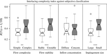
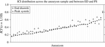
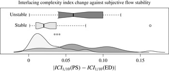
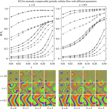
Figures 7, 9, 11 and 15 show the ICI obtained for different types of geometries and flows, which are described in the following sections. Each of them is presented together with a corresponding illustration of the complexity introduced by the interlacing of the streamlines when propagating from the inlet to the outlet. This provides an intuitive understanding of the meaning of the proposed ICI as a flow complexity quantification.
Observe that all the elements involved in the definition of the ICI are valid for an inlet and outlet of any geometry and topology. In particular, inlet and outlet may consist of multiple, separate regions. which would be analogous to a multiple-inputs multiple-outputs (MIMO) communication system.
4 Numerical experiments design
4.1 Flow cases
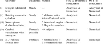
In §§ 5–8, we present several numerical experiments involving five different flow cases. Their characteristics are summarized in table 1. They illustrate a diversity of geometries and flow conditions, including steady and unsteady flows, and different inlet and outlet geometries and topologies. In all cases, except for case (v), rigid impermeable walls and incompressible Newtonian flow is assumed.
Depending on the case, the flow fields and streamlines have been obtained analytically or by numerical simulation and integration. For the simplest case (i), flow field, streamlines and MI have been computed both analytically and numerically. This have been used in § 5 to estimate the accuracy of the algorithms and to test the correctness of their implementation. Cases (ii) and (iii) represent idealized geometries and steady flows, and their corresponding ICI under different conditions is investigated in § 6. In contrast, case (iv) includes anatomically realistic vasculatures and unsteady flows, which are presented and investigated in § 7. A subset of them has been also used in § 5 to evaluate the algorithm accuracy in more complex cases. Case (v) is analytically defined and represents a family of unsteady compressible 2-D periodic cellular flows. In § 8, we analyse the obtained
 $\mathit{ICI}_{s}$
for different parameter values and test its limit for infinitesimal scales.
Summary of the characteristics of the 4 flow cases considered for the numerical experiments.

4.2 Flow simulations
From the surface triangular meshes representing the different geometries, unstructured volumetric meshes have been created using an octree approach with ICEM CFD 13.0 (ANSYS, Canonsburg, PA, USA). The considered geometries have a typical radius of
 $2~\text{mm}$
, and the resulting meshes are composed of tetrahedral elements with a side length of 0.24 mm and, at the wall, three layers of prism elements with a total height of
 $0.08~\text{mm}$
and a side length of
 $0.12~\text{mm}$
. This mesh configuration was selected according to the mesh convergence study performed in the project @neurist (Aneurist Consortium 2010; Villa-Uriol et al.
Reference Villa-Uriol, Berti, Hose, Marzo, Chiarini, Penrose, Pozo, Schmidt, Singh and Lycett2011).
The flow fields have been simulated with the vertex-centred finite volume solver CFX 13.0 (ANSYS) for Navier–Stokes equations, using a second-order advection scheme, a second-order backward Euler transient scheme for unsteady simulations and CFX’ automatic time scale control for steady-state simulations. An incompressible Newtonian fluid with viscosity
 $\unicode[STIX]{x1D707}=3.5~\text{mPa s}$
and density
 $\unicode[STIX]{x1D70C}=1066~\text{kg}~\text{m}^{-3}$
(typical values for blood) was considered.
Rigid walls, volumetric inflow rate and parabolic velocity profile in the inlet, with moderate Reynolds numbers (
 $\mathit{Re}\leqslant 500$
), have been imposed as boundary conditions. Steady flows have been simulated for the straight (i) and the double-bend tubes (iii), with a maximum residual of
 $10^{-5}$
.
Unsteady cyclic flow has been simulated for the arteries with aneurysm (iv). The specific boundary conditions at the inlet (flow rate) and outlets (pressure) were computed for a cardiac cycle using a one-dimensional model of the human vascular tree (Reymond et al.
Reference Reymond, Merenda, Perren, Rüfenacht and Stergiopulos2009). The cardiac cycle, with a period of 0.8 s, has been discretized in 160 uniformly distributed time steps (
 $5~\text{ms}$
) and, to reduce the effect of initial transients, the third of three simulated cardiac cycles has been analysed. A maximum residual of
 $5\times 10^{-3}$
was set as convergence criterion. This corresponds to the state-of-the art protocol for haemodynamic simulation studies defined in the @neurist project. Although not strictly converged in some cases, it represents a balance between accuracy and computational time, being sufficient to illustrate how the ICI could be used in practical applications. The protocol and convergence criterion is stricter for the idealized flow simulations.
For cases (ii) and (v) the flow fields are obtained analytically.
4.3 Streamlines computation
From the flow velocity fields, the streamlines have been obtained by numerical integration using a fourth-order Runge–Kutta algorithm, implemented in the Visualization ToolKit library (Schroeder, Martin & Lorensen Reference Schroeder, Martin and Lorensen2003; VTK community 2014). The integration is controlled by the length step, which we have set to of
 $1/20$
of the cell length. Inside each cell the velocity is linearly interpolated from the values at the cell nodes. The integration is terminated if either the number of steps reach
 $10^{5}$
or the speed is below
 $10^{-100}~\text{m}~\text{s}^{-1}$
. Observe that this termination speed will be virtually never reached, since those stagnant streamlines have null probability according to the natural distribution of streamlines.
The seed points are selected according to the natural distribution (2.8) in either inlet or outlet. The streamlines are propagated in both directions, forwards and backwards. In the inlet case, recirculation is controlled by discarding any seed point for which the backwards propagated streamline crosses again the inlet. In the outlet case, the seed is discarded if the forwards propagated streamline crosses again the outlet. This algorithm implements definition 3 of inlet and outlet.
The streamlines sample is generated on the fly from the flow field while computing the MI. In order to reduce the memory consumption, they are generated in groups of 2k. Then, the inlet and outlet crossings,
 $\boldsymbol{x}_{In}(\unicode[STIX]{x1D6FE})$
and
 $\boldsymbol{x}_{Out}(\unicode[STIX]{x1D6FE})$
, are identified and the streamlines are removed to free memory. For the different experiments, MI has been computed from sets of streamlines going from 5k to 100k.
4.4 ICI estimation
The joint probability density (3.2) can be estimated from a sample of
 $N$
streamlines,
 $\{\unicode[STIX]{x1D6FE}_{\unicode[STIX]{x1D6FC}}\}$
, generated from any flow cross-section (in particular, either inlet or outlet) with the natural probability density (2.8):
 $$\begin{eqnarray}p_{s}(\boldsymbol{x},\boldsymbol{y})\simeq \frac{1}{N}\mathop{\sum }_{\unicode[STIX]{x1D6FC}=1}^{N}p_{In,s}(\boldsymbol{x}\mid \unicode[STIX]{x1D6FE}_{\unicode[STIX]{x1D6FC}})\,p_{Out,s}(\boldsymbol{y}\mid \unicode[STIX]{x1D6FE}_{\unicode[STIX]{x1D6FC}}).\end{eqnarray}$$
The factor
 $p(\unicode[STIX]{x1D6FE})$
disappears because it is taken into account when generating the sample of streamlines. Then, Monte Carlo integration (Robert & Casella Reference Robert and Casella2013) is applied for the computation of the MI in (3.3), using uniform samplings of
 $M$
points in both the inlet and the outlet. The same procedure is applied for the estimation of
 $I_{s}(\boldsymbol{X},\boldsymbol{Y})$
,
 $I_{s}(\boldsymbol{X},\boldsymbol{X})$
and
 $I_{s}(\boldsymbol{Y},\boldsymbol{Y})$
. From them,
 $\mathit{ICI}_{s}$
is computed as defined in (3.8). For computation and memory efficiency, the PSF is truncated for distances
 ${>}3.717\unicode[STIX]{x1D70E}$
, corresponding to the 99.9 % confidence region, and sparse matrices are used in the algorithm.
This algorithm is linear in the number of streamlines,
 $N$
, and quadratic in the number of points,
 $M$
. The complete algorithm, including the streamlines computation, has been implemented in C++. All the experiments have been run in a MacBook Pro, 2.8 GHz dual-core Intel Core i7, 16 GB SDRAM. The mean computational time for the full process, from flow field to
 $\mathit{ICI}_{s}$
, for the scale sequence
 $s=1/3,1/4,\ldots ,1/20$
, with
 $N=20\text{k}$
and
 $M=5\text{k}$
, was 5 min. But this time depends on the geometry extent and the flow complexity.
5 Accuracy, precision and invariance
5.1 Algorithm accuracy and precision evaluation
To check the correctness and accuracy of the algorithm described above for the estimation of the ICI, we have considered the steady flow in a cylindrical straight tube (i) and the pulsatile flow in a subset of the dataset of anatomically realistic vasculatures with aneurysm (iv).
For case (i), the MI can be semi-analytically computed. This computation and the resulting values for
 $I_{s}(\boldsymbol{X},\boldsymbol{Y})$
are presented in appendix A. Alternatively, the corresponding MI has been also numerically computed from the flow simulated for a tube of radius
 $R=2~\text{mm}$
and length
 $L=0.3~\text{m}$
, and a flow rate
 $Q=5~\text{ml}~\text{s}^{-1}$
, corresponding to
 $\mathit{Re}=485$
.
 $I_{s}(\boldsymbol{X},\boldsymbol{Y})$
has been estimated for a series of streamline samples of sizes
 $N=5\text{k},10\text{k},20\text{k},50\text{k}$
, and of point samples of sizes
 $M=2\text{k},5\text{k},10\text{k},20\text{k}$
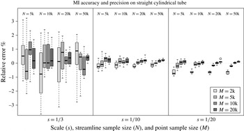
. Each combination has been instantiated 8 times to evaluate also their variability. The resulting values have been compared with the semi-analytical computation, considered as the ground truth (GT). Figure 4 presents the distribution of signed relative errors,
 $(I_{s}-I_{s}^{(GT)})/I_{s}^{(GT)}$
, obtained with the different sample sizes, for scales
 $s=1/3,1/10,1/20$
.
Evaluation of the accuracy and precision of the algorithm implementation for the computation of the MI. For a stationary flow in a cylindrical straight tube, the numerical estimation is compared with the semi-analytical computation. The signed error is evaluated for 3 scales (
 $s$
), 4 streamline sample sizes (
 $N$
) and 4 point sample sizes (
 $M$
).

To estimate the algorithm precision and accuracy in more complex geometries and flows, we have selected a random subset of 10 cases from the dataset of cerebral vasculatures with aneurysms (iv), considering their
 $\mathit{ICI}_{s}$
computed from the streamlines at one cardiac phase (peak systole). Since no analytical ground truth is available in this case, each
 $\mathit{ICI}_{s}$
has been computed using
 $N=100\text{k}$
streamlines and
 $M=50\text{k}$
points, which is in the limit of the feasible computation, needing for each case 20 h of computation with peaks of 15 GB of memory usage. The obtained values have been taken as ground truth. The ICI has been also computed for
 $N=5\text{k},10\text{k},20\text{k},50\text{k}$
and
 $M=2\text{k},5\text{k},10\text{k},20\text{k}$
, instantiated twice for each combination. For each scale, the signed error is given by the difference with respect to the ground truth,
 $\unicode[STIX]{x1D700}_{s}=\mathit{ICI}_{s}-\mathit{ICI}_{s}^{(GT)}$
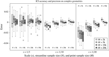
. Since the ICI is normalized between 0 and 1, this absolute error is directly interpretable as relative to the index range and comparable between scales. Figure 5 presents the obtained distribution of errors. Table 2 presents the estimated accuracy and precision for 3 different settings for
 $N$
and
 $M$
, where the accuracy is quantified by the mean signed error,
 $\overline{\unicode[STIX]{x1D700}}$
, and the precision by twice its standard deviation,
 $2\unicode[STIX]{x1D70E}_{\unicode[STIX]{x1D700}}$
, representing approximately the 95 % confidence interval (
 $\overline{\unicode[STIX]{x1D700}}\pm 2\unicode[STIX]{x1D70E}_{\unicode[STIX]{x1D700}}$
).
Evaluation of the accuracy and precision of
 $\mathit{ICI}_{s}$
computation on the flow at peak systole in 10 vasculatures with aneurysm. For each scale (
 $s$
), the signed error against the ground truth is evaluated for several streamline sample sizes (
 $N$
) and point sample sizes (
 $M$
).

Accuracy (
 $\overline{\unicode[STIX]{x1D700}}$
) and precision (
 $2\unicode[STIX]{x1D70E}_{\unicode[STIX]{x1D700}}$
) of
 $\mathit{ICI}_{s}$
for 3 scales and 3 settings of
 $N$
and
 $M$
, estimated from the flow in 10 vasculatures with aneurysm. The values are expressed as
 $\overline{\unicode[STIX]{x1D700}}\pm 2\unicode[STIX]{x1D70E}_{\unicode[STIX]{x1D700}}$
(approximate 95 % confidence interval).

As expected, both accuracy and precision increase with the number of streamlines (
 $N$
) and with the number of points (
 $M$
). For the straight tube, the convergence to the semi-analytical values evidences the correctness of the algorithm implementation.
The accuracy is degraded from coarser scales (large
 $s$
) to finer scales (small
 $s$
), and from larger samples sizes,
 $N$
and
 $M$
, to smaller ones. This bias for small samples is a known effect for experimental MI estimators (Paninski Reference Paninski2003). It is interesting that the bias introduced by small
 $N$
and
 $M$
acts in opposite directions. Reducing the number of streamlines (
 $N$
) should presumably reduce the apparent complexity, which explains the observed decrease in the ICI (figure 5), specially for
 $s=1/20$
. Accordingly, this bias dependence with
 $N$
is not observed for the simple flow in the straight tube (figure 4). For smaller
 $s$
, the area covered by the PSF is smaller, requiring denser samples. This explains the bias increase when
 $s$
decreases, for the same
 $N$
and
 $M$
.
The estimation of ICI is most precise for the intermediate scale, reducing the precision towards both extremes. Two competing effects appear here. The variability of the MI estimator increases for small sample sizes compared with the observation scale. Thus, for the same
 $N$
and
 $M$
, the MI variability decreases when
 $s$
increases. However, the ICI normalization factor also decreases, magnifying the ICI errors for the same MI errors.
From the obtained values, a reasonable selection seems to be
 $N=20\text{k}$
and
 $M=5\text{k}$
, involving an acceptable mean computational time of 5 min per case, representing a balance between accuracy and computational time and memory. Hence, these algorithm settings have been used in the subsequent experiments.
5.2 Streamline distribution invariance
Although the natural probability distribution of streamlines is analytically invariant to the cross-section generating them, this invariance can be broken by the numerical approximations involved in the flow simulations. As shown in § 2.3, the source of variation of the streamline distribution is the integral of the flow divergence,
 $\unicode[STIX]{x1D709}(\unicode[STIX]{x1D6FE})$
, along each streamline,
 $\unicode[STIX]{x1D6FE}$
, as defined in (2.18).
For testing this invariance and the influence of the numerical errors, we have considered the unsteady flow cases (iv) in cerebral vasculatures. For each case, 5 different streamline samples have been generated either forward from the inlet or backward from the outlet, and with either the natural or homogeneous distribution.
- (FNa)
-
Forward, natural distribution (Sample A).
- (FNb)
-
Forward, natural distribution (Sample B).
- (BN)
-
Backward, natural distribution.
- (FH)
-
Forward, homogeneous distribution.
- (BH)
-
Backward, homogeneous distribution.
Here, homogeneous denotes the distribution of streamlines obtained from a homogeneous sample of seed points at the inlet (forward) or outlet (backwards). It is used as a naive alternative against which to compare the natural distribution. The corresponding MI has been computed from each of these samples. The flow divergence has been also computed and integrated along each streamline, providing
 $\unicode[STIX]{x1D709}(\unicode[STIX]{x1D6FE})$
.
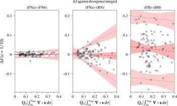
Figure 6 presents the MI difference,
 $\unicode[STIX]{x0394}I$
, between two streamlines samples (inter-sample variability) for 3 different pairs of samples: (FNa)–(FNb), (FNa)–(BN) and (FH)–(BH). The MI difference is plotted against the third quartile of the absolute value of the divergence integrals,
 $\tilde{\unicode[STIX]{x1D709}}=\text{Q}_{3}(|\unicode[STIX]{x1D709}(\unicode[STIX]{x1D6FE})|)$
. We have considered the linear model
 $\unicode[STIX]{x0394}I=a+b\tilde{\unicode[STIX]{x1D709}}+\unicode[STIX]{x1D700}+\unicode[STIX]{x1D6FD}\tilde{\unicode[STIX]{x1D709}}$
, with two independent normally distributed errors: a constant noise,
 $\unicode[STIX]{x1D700}\sim {\mathcal{N}}(0,\unicode[STIX]{x1D70E}_{\unicode[STIX]{x1D700}})$
, and an effect linearly increasing with the divergence integral,
 $\unicode[STIX]{x1D6FD}\tilde{\unicode[STIX]{x1D709}}\sim {\mathcal{N}}(0,\unicode[STIX]{x1D70E}_{\unicode[STIX]{x1D6FD}}\tilde{\unicode[STIX]{x1D709}})$
. The fitted line and 95 % confidence intervals for the differences, are given by the minimum likelihood estimates of the linear model parameter,
 $a$
,
 $b$
,
 $\unicode[STIX]{x1D70E}_{\unicode[STIX]{x1D700}}$
,
 $\unicode[STIX]{x1D70E}_{\unicode[STIX]{x1D6FD}}$
. The statistical significance of the dependency of the error with the divergence integral (
 $\unicode[STIX]{x1D70E}_{\unicode[STIX]{x1D6FD}}>0$
) has been further confirmed by the studentized Breusch–Pagan test (Koenker Reference Koenker1981).
Dependence of the inter-sample variability of the MI on the divergence integral. The differences are plotted for two streamline samples generated at the inlet (FNa–FNb), sample at the inlet minus sample at the outlet generated by the natural distribution of streamlines (FNa–BN) and generated by homogeneous distribution (FH–BH).

As expected, the difference,
 $\unicode[STIX]{x0394}I$
, for two samples equally generated from the inlet, (FNa)–(FNb), shows no bias and the 95 % confidence interval is independent of the divergence integral.
For (FNa)–(BN),
 $\unicode[STIX]{x0394}I$
shows a bias and a 95 % confidence interval significantly dependent on the divergence integral (
 $p=6\times 10^{-6}$
). But the limit for null divergence coincides with the differences obtained from (FNa)–(FNb). This is in agreement with the expected invariance of the natural distribution of streamlines with respect to the generating cross-section.
In contrast, for (FH)–(BH), the 95 % confidence interval is independent of
 $\tilde{\unicode[STIX]{x1D709}}$
and significantly larger than the confidence interval for (FNa)–(FNb). This reflects the importance of using the natural distribution of streamlines.
6 ICI along steady flows in simple geometries
6.1 Rotating concentric cylinders with axial flow
The flow resulting in the annulus between two concentric cylinders, of inner radius
 $R_{1}$
and outer radius
 $R_{2}$
, rotating with different angular velocities,
 $\unicode[STIX]{x1D714}_{1}$
and
 $\unicode[STIX]{x1D714}_{2}$
respectively, is a well-studied case with a long history (Childs Reference Childs2010). In general, the flow can be unstable involving Taylor vortices. For low angular velocity or high viscosity, with Reynolds and Taylor numbers below a critical value, the steady flow is cylindrically symmetric and can be expressed analytically. For the case with static outer cylinder,
 $\unicode[STIX]{x1D714}_{2}=0$
, and a constant pressure gradient in the axial direction,
 $\unicode[STIX]{x2202}p/\unicode[STIX]{x2202}z=-p^{\prime }$
, a steady incompressible Newtonian flow under no-slip condition can be expressed in cylindrical coordinates as
 $$\begin{eqnarray}\displaystyle v^{z}=\frac{p^{\prime }{R_{2}}^{2}}{4\unicode[STIX]{x1D707}}\left(1-\hat{r}^{2}-\frac{1-k^{2}}{\log k}\log \hat{r}\right),\quad v^{\unicode[STIX]{x1D703}}=\frac{\unicode[STIX]{x1D714}_{1}k^{2}R_{2}}{1-k^{2}}\frac{1-\hat{r}^{2}}{\hat{r}},\quad v^{r}=0, & & \displaystyle\end{eqnarray}$$
where
 $k=R_{1}/R_{2}$
and
 $\hat{r}=r/R_{2}$
. This velocity field can be integrated to obtain the streamlines:
 $$\begin{eqnarray}\displaystyle \unicode[STIX]{x1D703}(t)=\unicode[STIX]{x1D703}_{0}+\frac{v^{\unicode[STIX]{x1D703}}}{r}t,\quad z(t)=z_{0}+v^{z}t,\quad r(t)=r_{0}. & & \displaystyle\end{eqnarray}$$
Thus, for inlet and outlet defined by the cross-sections at
 $z=z_{In}$
and
 $z=z_{In}+L$
, a streamline crossing the inlet at
 $(r_{In},\unicode[STIX]{x1D703}_{In},z_{In})$
, will cross the outlet at
 $(r_{Out},\unicode[STIX]{x1D703}_{Out},z_{Out})$
, where
 $$\begin{eqnarray}r_{Out}=r_{In},\quad \unicode[STIX]{x1D703}_{Out}=\unicode[STIX]{x1D703}_{In}+L\frac{v^{\unicode[STIX]{x1D703}}}{rv^{z}},\quad z_{Out}=z_{In}+L.\end{eqnarray}$$
The local flux at the inlet or outlet is given by
 $\unicode[STIX]{x1D711}_{\boldsymbol{v}}^{{\mathcal{S}}}=v^{z}$
, which gives the total volumetric flow rate
 $$\begin{eqnarray}\displaystyle Q=\frac{p^{\prime }{R_{2}}^{2}}{4\unicode[STIX]{x1D707}}A\,C,\quad \text{where}~C=\frac{1}{2}\left(1+k^{2}+\frac{1-k^{2}}{\log k}\right), & & \displaystyle\end{eqnarray}$$
and
 $A=\unicode[STIX]{x03C0}({R_{2}}^{2}-{R_{1}}^{2})$
is the cross-sectional area. After normalization we obtain the natural probability density of streamlines
 $$\begin{eqnarray}p(\unicode[STIX]{x1D6FE})=\frac{1}{A\,C}\left(1-\hat{r}^{2}-\frac{1-k^{2}}{\log k}\log \hat{r}\right).\end{eqnarray}$$
Finally, expanding
 $v^{\unicode[STIX]{x1D703}}$
and
 $v^{z}$
in (6.3), we get
 $$\begin{eqnarray}\unicode[STIX]{x1D703}_{Out}=\unicode[STIX]{x1D703}_{In}+\unicode[STIX]{x1D706}\,\frac{\unicode[STIX]{x03C0}C}{\hat{r}^{2}}\left(1-\frac{(1-k^{2})\log \hat{r}}{(1-\hat{r}^{2})\log k}\right)^{-1},\quad \text{with}~\unicode[STIX]{x1D706}=\frac{\unicode[STIX]{x1D714}_{1}R_{1}^{2}L}{Q}.\end{eqnarray}$$
Observe that
 $\unicode[STIX]{x1D706}$
is a dimensionless quantity, which can be interpreted as the product of two ratios:
 $$\begin{eqnarray}\displaystyle \unicode[STIX]{x1D706}=\frac{\mathit{Ta}}{\mathit{Re}}\,\frac{R_{1}L}{A}=\frac{v_{1}^{\unicode[STIX]{x1D703}}}{\overline{v}^{z}}\,\frac{R_{1}L}{A}, & & \displaystyle\end{eqnarray}$$
where the Taylor number (or rotational Reynolds number),
 $\mathit{Ta}$
, and the (axial) Reynolds number,
 $\mathit{Re}$
, are defined as in Lueptow, Docter & Min (Reference Lueptow, Docter and Min1992) and Wereley & Lueptow (Reference Wereley and Lueptow1999), so that their ratio is the quotient of the velocity of the interior cylinder,
 $v_{1}^{\unicode[STIX]{x1D703}}=\unicode[STIX]{x1D714}_{1}R_{1}$
, by the bulk axial velocity,
 $\overline{v}^{z}=Q/A$
.
We have run experiments for three values of the ratio between internal and external radius,
 $k=0.1$
, 0.5 and 0.8, and an exponential sequence of values for
 $\unicode[STIX]{x1D706}$
, ranging along several orders of magnitude from 0.01 to 100. For each value of
 $k$
and
 $\unicode[STIX]{x1D706}$
, a sample of crossing points at the inlet and outlet from
 $20$
k streamlines have been generated following (6.5) and (6.6). The corresponding ICI has then been computed from each of these samples.
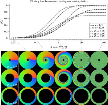
Figure 7 shows the evolution of ICI when
 $\unicode[STIX]{x1D706}$
increases, for two scales,
 $s=1/3$
and
 $1/20$
, and for the three radius ratios. Different combinations of fluid properties or boundary conditions can result in the same value of
 $\unicode[STIX]{x1D706}$
. Two simple interpretations of the curves are that they represent either the ICI evolution when increasing the distance,
 $L$
, from inlet to outlet, or the ICI change when increasing the rotational velocity,
 $\unicode[STIX]{x1D714}_{1}$
.
Figure 7 also illustrates the degree of mixing by rendering how the azimuthally coloured inlet is propagated by the streamlines, producing deformed images by their intersection at the outlet. This gives an intuition of the mixing corresponding to each value of the ICI.
The ICI increases faster and further for coarser scales. In particular,
 $\mathit{ICI}_{1/3}$
converges very close to 1 for large
 $\unicode[STIX]{x1D706}$
, while
 $\mathit{ICI}_{1/20}$
is always below 0.9. At first glance, we could expect that
 $\mathit{ICI}_{s}$
converges to 1 for any scale. However, this laminar rotating flow produces no mix in the radial direction. Thus, there is always some amount of information preserved. The difference between both scales is larger for the smallest radius ratio,
 $k=0.1$
, while for
 $k=0.8$
the ICI of both scales approach each other. The value of
 $\mathit{ICI}_{s}$
also increases with
 $k$
, since then the contribution of the radial direction is reduced with respect to the angular one.
ICI and illustration of the mixing produced by a steady flow in annulus with rotating inner cylinder and axial pressure gradient, for 3 radius ratios. The ICI at two scales (
 $s$
) is plotted as function of the dimensionless parameter
 $\unicode[STIX]{x1D706}$
. For each radius ratio, the azimuthally coloured inlet (left column) is propagated by the streamlines, producing deformed images by their intersection at the outlet for
 $\unicode[STIX]{x1D706}=0.01$
,
 $0.1$
,
 $1$
,
 $10$
and
 $100$
.

6.2 Double-bend tubes
One of the simplest 3-D geometries is a tube including the sequence of two non-coplanar
 $90^{\circ }$
bends. Lee et al. (Reference Lee, Parker, Caro and Sherwin2008) investigated the characteristics of the steady flow obtained under 5 different inter-bend angles (
 $\unicode[STIX]{x1D6FC}=0^{\circ },45^{\circ },90^{\circ },135^{\circ },180^{\circ }$
) and 2 Reynolds numbers (
 $\mathit{Re}=125,500$
), with tube radius
 $R=2~\text{mm}$
and bend radius
 $R_{bend}=8~\text{mm}$
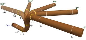
. We have reproduced the same geometries (figure 8) and flow conditions considered there, investigating the ICI obtained in each case.
For each angle, a series of cross-sections have been generated every
 $1~\text{mm}$
along the tube centreline, numbered according to their position relative to the inter-bend centre (see figure 8). The ICI has been computed from the inlet cross-section at
 $-30~\text{mm}$
, to each of the outlets in the cross-section series, from position
 $-20~\text{mm}$
to
 $40~\text{mm}$
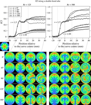
. Figure 9 shows the ICI obtained along this sequence of outlets, for the 5 angles and 2 Reynolds numbers and for 2 scales:
 $s=1/3$
and
 $1/20$
.
Double-bend tubes with inter-bend angles
 $0^{\circ }$
,
 $45^{\circ }$
,
 $90^{\circ }$
,
 $135^{\circ }$
and
 $180^{\circ }$
. For each angle, a series of cross-sections have been generated along the tube centreline, each separated 1 mm from the previous one. They are numbered according to their position relative to the inter-bend centre. The inter-bend centre (
 $0$
), the first ring at the beginning of the first bend (
 $-12$
) and the last ring at the end of the second bend (
 $12$
) are shown in yellow.

The inlet has been coloured radially from red in the centre to blue in the perimeter, adding 6 white radius. This image was propagated by the flow streamlines, producing deformed images by their intersection with each cross-section. These images illustrates the degree of mixing and complexity of the flow from the inlet to each of the series of outlets. They are presented in figure 9 at positions
 $-$
5, 0, 12 and 40 mm, for each angle and Reynolds, together with the corresponding ICI.
ICI and illustration of the mixing along double-bend tubes with 5 different inter-bend angles, and for two Reynolds numbers. The corresponding
 $\mathit{ICI}_{s}$
is computed for two scales,
 $s=1/3$
(circles) and
 $s=1/20$
(triangles), from the inlet to each of the outlets in the cross-section series (see figure 8). To visualize the degree of mixing, the radially coloured inlet is propagated by the streamlines, producing deformed images by their intersection with each cross-section. They are presented at positions
 $-5$
,
 $0$
,
 $12$
and
 $40$
mm, for each angle and Reynolds number.

When comparing the 5 angles, both the coloured cross-sections and the ICI coincide for outlets along the first bend and the initial portion of the second bend, where the dynamics is essentially characterized by the Dean vortices developed by the first bend. The divergence between angles starts earlier for
 $\mathit{Re}=500$
, as seen in both scales. This can be explained since the Dean vortices generated by the second bend are stronger and faster developed for higher Reynolds number.
The ICI for the planar bend with
 $\unicode[STIX]{x1D6FC}=180^{\circ }$
is almost the same for both Reynolds numbers at the end of the second bend (
 $12~\text{mm}$
). This can be understood since the higher energy in the Dean vortices for
 $\mathit{Re}=500$
is compensated by the higher axial velocity, so that the streamlines are similar. Lee et al. (Reference Lee, Parker, Caro and Sherwin2008) mention that at
 $\mathit{Re}=500$
the strength of the primary Dean vortices is sufficient to lead to secondary and even tertiary vortices. They do not explicitly state this not happening at
 $\mathit{Re}=125$
, but any possible differences between both does not result in a clear difference in ICI. However, the ICI still grows significantly after the second bend for
 $\mathit{Re}=500$
, indicating that the vortices are more persistent. This effect is common also for all the angles, so that the ICI at
 $40~\text{mm}$
is always larger for
 $\mathit{Re}=500$
, and not even completely developed, in contrast with
 $\mathit{Re}=125$
.
As expected, the ICI at the outlet is higher for non-planar than for planar models. Both
 $\unicode[STIX]{x1D6FC}=45^{\circ }$
and
 $\unicode[STIX]{x1D6FC}=90^{\circ }$
present very similar coloured cross-sections and ICI. They share the highest ICI in both scales and both Reynolds numbers. This is in agreement with the observation in Lee et al. (Reference Lee, Parker, Caro and Sherwin2008) that there appears to be an optimal inter-bend angle between
 $45^{\circ }$
and
 $90^{\circ }$
to achieve asymmetry in the Dean vortex pattern.
In contrast with
 $\unicode[STIX]{x1D6FC}=180^{\circ }$
, for
 $\unicode[STIX]{x1D6FC}=0^{\circ }$
the ICI is substantially higher at
 $\mathit{Re}=500$
than at
 $\mathit{Re}=125$
. Apparently the reverse Dean vortices developed in the second bend, partially undo the mixing for low Reynolds number. This even produces a reduction of ICI for
 $\mathit{Re}=125$
at the end of the second bend. This effect can be seen in the coloured cross-sections, with the reduction of the deformation in the centre at
 $12~\text{mm}$
.
For
 $\mathit{Re}=125$
, we can also observe a small reduction of the ICI at the end of the first bend, only for scale
 $s=1/3$
, but shared by all the angles. We have not found a satisfactory explanation of this effect.
7 Unsteady incompressible flow on complex geometries
7.1 Cerebral arteries with aneurysms
As a case study on non-idealized geometries, we have investigated the ICI obtained for unsteady flows in anatomically realistic cerebral arteries with aneurysms. Aneurysms are pathologic dilations of the vessel wall, and their flow characteristics have been extensively investigated as mechanically and biologically related with the initiation, growth and eventual rupture of aneurysms (Cebral et al. Reference Cebral, Mut, Weir and Putman2011; Geers et al. Reference Geers, Larrabide, Radaelli, Bogunovic, Kim, van Andel, Majoie, VanBavel and Frangi2011; Gopalakrishnan, Pier & Biesheuvel Reference Gopalakrishnan, Pier and Biesheuvel2014; Schnell et al. Reference Schnell, Ansari, Vakil, Wasielewski, Carr, Hurley, Bendok, Batjer, Carroll and Carr2014; Arzani et al. Reference Arzani, Gambaruto, Chen and Shadden2016).
A set of 49 geometries obtained from segmentation of 3-D rotational angiography (3DRA) images including an aneurysm in the middle cerebral artery have been selected from the @neurIST database (Aneurist Consortium 2010; Villa-Uriol et al.
Reference Villa-Uriol, Berti, Hose, Marzo, Chiarini, Penrose, Pozo, Schmidt, Singh and Lycett2011). Surface models of patient-specific vascular geometries were obtained with the geodesic active region segmentation method (Bogunović et al.
Reference Bogunović, Pozo, Villa-Uriol, Majoie, van den Berg, Gratama van Andel, Macho, Blasco, San Román and Frangi2011) and manually corrected for topological errors using the software suite @neuFuse (Villa-Uriol et al.
Reference Villa-Uriol, Berti, Hose, Marzo, Chiarini, Penrose, Pozo, Schmidt, Singh and Lycett2011). The vasculature of interest includes at least 12 vessel diameters upstream and 4 vessel diameters downstream from the aneurysm. Inlets and outlets have been clipped with planes perpendicular to the vessel centreline. Unsteady flow simulations have been performed imposing flow rate (inlet) and pressure waveforms (outlets) extracted from a one-dimensional model of all the large arteries in the human body (Reymond et al.
Reference Reymond, Merenda, Perren, Rüfenacht and Stergiopulos2009), for a cardiac cycle of period
 $0.8~\text{s}$
.
For the resulting unsteady incompressible flow, both versions of ICI could be applied: considering either streamlines or world-lines. We have considered here the streamlines for two physiologically relevant cardiac phases: peak systole (PS) and end diastole (ED). This allows us to directly compare the results to some existing subjective classifications of aneurysm flow complexity and stability, defined also for these two cardiac phases.
The considered control volume,
 ${\mathcal{D}}_{{\mathcal{S}}}$
, comprises the aneurysm and a portion of each adjacent vessel. We have selected inlet and outlet at one vessel diameter from the aneurysm neck, as illustrated in figure 10. This is the same criterion introduced by Millan et al. (Reference Millan, Dempere-Marco, Pozo, Cebral and Frangi2007) for aneurysm morphological characterization. The limiting cross-sections were automatically computed based on the aneurysm removal methodology proposed by Ford et al. (Reference Ford, Hoi, Piccinelli, Antiga and Steinman2009) and implemented in the Vascular Modelling Toolkit (Piccinelli et al.
Reference Piccinelli, Veneziani, Steinman, Remuzzi and Antiga2009). Using vessel centrelines and Voronoi diagrams, the aneurysm neck and vessel bifurcations were detected and used as a reference to reliably identify the cross-sections.
For this control volume, the outlet consists of multiple, separate regions. But this does not affect the definition of ICI.
Example of the cross-sections automatically selected for the inlet vessel and each of the two outlet vessels, at one diameter from the aneurysm neck at the bifurcation.

7.2 ICI as a function of scale
For each case,
 $\mathit{ICI}_{s}$
was obtained for the sequence of scales,
 $s=1/3,1/4,\ldots ,1/20$
. This provides ICI as a function of the scale. Figure 11, displays this function for several representative examples.
ICI as function of scale and illustration of mixing in typical cases from the aneurysm dataset. The line-connected symbols are the ICI at PS of examples representing the minimum, maximum, median and first and third quartiles, for
 $s=1/20$
. The case with largest change in the order from
 $s=1/3$
to
 $s=1/20$
pass from the first to the fourth quartile. The ICI mean, and the variation explained by the first 2 principal components are also plotted. Each of the outlets have been coloured by two different patterns: by homogenous colour identifying each outlet vessel as blue or red, and radially with a rainbow colour map. Their propagation backwards by the streamlines produces respectively two coloured cross-sections at the inlet.

In general,
 $\mathit{ICI}_{s}$
increases with the scale
 $s$
. The obtained continuous and smooth behaviour makes evident a high correlation between the values at different scales. Thus, a dimensionality reduction can be obtained, for instance, by principal component analysis. Effectively, the first principal component (PC) explains 99.1 % of the variance, and the 2 first PCs explain 99.9 % of the variance. These two PCs are also plotted in figure 11.
An illustration of the mixing corresponding to each of the ICI values is also presented by coloured cross-sections, similar to the ones in previous cases, but adapted to the multiplicity of the outlet. Each of the outlets have been coloured by two different patterns: radially from red to blue, and by homogenous colour identifying each outlet vessel. Two coloured cross-section are respectively obtained at the inlet, by their propagation backwards along the streamlines.
7.3 Comparison with subjective assessment of flow complexity
For each aneurysm, the flow field has been qualitatively assessed by an expert, through visual inspection of the streamlines, according to four qualitative variables (Cebral et al. Reference Cebral, Mut, Weir and Putman2011; Geers et al. Reference Geers, Larrabide, Radaelli, Bogunovic, Kim, van Andel, Majoie, VanBavel and Frangi2011). Three variables are measured at PS: flow complexity (simple or complex), inflow concentration (concentrated or diffuse) and impingement size (small or large). The fourth variable, flow stability (stable or unstable), is measured by comparing the flow patterns at PS and ED.
We have investigated the correlation of the proposed quantitative ICI at PS with the subjective qualitative classification. For each qualitative variable, the corresponding two categories have been plotted as a box plot of
 $\mathit{ICI}_{1/10}$
(figure 12). Non-parametric Mann–Whitney
 $U$
test (Mann & Whitney Reference Mann and Whitney1947; Hollander, Wolfe & Chicken Reference Hollander, Wolfe and Chicken2013) has been applied to each pair of categories. Three of them gave statistically significant differences (flow complexity:
 $p=9\times 10^{-3}$
, flow stability:
 $p=2\times 10^{-4}$
, impingement size:
 $p=4\times 10^{-4}$
). Only inflow concentration did not show significant differences. Surprisingly, flow stability showed significant differences for the ICI exclusively measured at PS, although it is supposed to account for the variation between ED and PS. Probably, this reflects the fact that more complex flows are also more unstable.
Correlation of ICI with each of the 4 subjective flow classifications. The significant difference between each pair of categories is assessed by non-parametric Mann–Whitney
 $U$
test.
 $^{\ast \ast }(0.01\geqslant p>0.001)$
,
 $^{\ast \ast \ast }(0.001\geqslant p>0.0001)$
.

7.4 Comparison between peak systole and end diastole
Figure 13 presents a dot plot with
 $\mathit{ICI}_{1/10}$
obtained for each aneurysm at PS and ED. The values spread quite homogeneously across the ICI range. In general, the ICI obtained for PS is larger than the one obtained for ED, but the opposite behaviour is also observed.
Comparison between ICI of the flow at peak systole and end diastole for each aneurysm, at scale
 $s=1/10$
. The ICI is generally larger at PS than at ED, but the opposite behaviour is also observed. The aneurysms have been ordered according to their ICI at ED.

The ICI variation from ED to PS is presented in figure 14, separated according to the qualitative classification into stable and unstable. A clear correlation appears, which is confirmed by one-tailed Mann–Whitney
 $U$
test, giving a high significant difference (
 $p=5\times 10^{-4}$
). For completeness, Mann–Whitney test was also applied to the ICI variation for the classes obtained from the qualitative flow complexity, inflow concentration and impingement size. None of them provided significant differences.
Subjective flow stability classes against absolute value of the difference of ICI between peak systole and end diastole. A strong significant difference (
 $p=0.0005$
, one-tailed Mann–Whitney
 $U$
test) is found between subjectively stable and unstable flows.

8 Unsteady compressible 2-D periodic cellular flows
8.1 Two-dimensional periodic cellular flows
Periodic cellular flows are simply defined models that can, however, show very complex evolutions. We have considered a modification of the 2-D unsteady model used by Zu, Chen & Xin (Reference Zu, Chen and Xin2015):
 $$\begin{eqnarray}\displaystyle \boldsymbol{v}=\frac{1}{\unicode[STIX]{x1D70C}}[(\cos (2\unicode[STIX]{x03C0}y),\cos (2\unicode[STIX]{x03C0}x))+\unicode[STIX]{x1D703}\cos (t)(\sin (2\unicode[STIX]{x03C0}y),\sin (2\unicode[STIX]{x03C0}x))] & & \displaystyle\end{eqnarray}$$
defined in Cartesian coordinates
 $\boldsymbol{x}=(x,y)$
for the square domain
 $\unicode[STIX]{x1D6FA}=[0,1]\times [0,1]$
with periodic boundary conditions (torus). The base flow (
 $\unicode[STIX]{x1D70C}=1,\unicode[STIX]{x1D703}=0$
) produce two counter-rotating cells centred at
 $(1/4,3/4)$
and
 $(3/4,1/4)$
, and two saddles at
 $(1/4,1/4)$
and
 $(3/4,3/4)$
. The parameter
 $\unicode[STIX]{x1D703}$
introduce a time-dependent perturbation, making it an unsteady flow. The original model did not include the density
 $\unicode[STIX]{x1D70C}$
. We have considered a density
 $$\begin{eqnarray}\displaystyle \unicode[STIX]{x1D70C}=1+\unicode[STIX]{x1D705}\sin (2\unicode[STIX]{x03C0}x)\sin (2\unicode[STIX]{x03C0}y) & & \displaystyle\end{eqnarray}$$
controlled by the parameter
 $\unicode[STIX]{x1D705}$
, which introduces an inhomogeneity, making the flow compressible. This density is maximum at the saddles and minimum at the rotating centres. The resulting unsteady compressible flow satisfies the continuity equation (2.28). Thus, the natural distribution of world-lines is invariant, and we can consider the corresponding version of ICI.
For this flow, we consider the spatio-temporal control volume
 ${\mathcal{D}}_{{\mathcal{S}}}=\unicode[STIX]{x1D6FA}\times {\mathcal{T}}$
given by the full spatial cyclic domain
 $\unicode[STIX]{x1D6FA}$
(torus) along a lapse of time
 ${\mathcal{T}}=[0,T]$
. Thus, the inlet and outlet are not spatial surfaces, but the full space,
 $\unicode[STIX]{x1D6FA}$
, at instances
 $t=0$
and
 $t=T$
, respectively.
Figure 15 illustrates the resulting flow for different values of
 $\unicode[STIX]{x1D703}$
and
 $\unicode[STIX]{x1D705}$
, and for different time lapses. The ICI for each of these parameter values and time lapses is displayed for a series of scales from
 $s=0.01$
to
 $s=0.5$
. The flow propagation of a vertical colour pattern is also shown for each of the parameter values.
ICI as a function of scale for the 2-D periodic cellular flow with
 $\unicode[STIX]{x1D705}=0$
(incompressible) and
 $\unicode[STIX]{x1D705}=0.9$
(compressible), with 4 different values of
 $\unicode[STIX]{x1D703}$
(unsteadiness) and for 3 time lapses. The legend is presented at the bottom, together with the illustration of the propagation by each flow of a vertical colour pattern.

The dominant factor is the increase of ICI with the time lapse. The increase of ICI with the parameter
 $\unicode[STIX]{x1D703}$
is pronounced for all scales and time lapses, reflecting that the higher the unsteadiness, the more complex the flow. The ICI for compressible flows (
 $\unicode[STIX]{x1D705}=0.9$
) is also higher than for incompressible flows (
 $\unicode[STIX]{x1D705}=0$
), although the difference is less marked. It is more evident for the steady flow (
 $\unicode[STIX]{x1D703}=0$
) and intermediate time (
 $t=1$
), for which the difference between steady and unsteady flow is reduced. This is in agreement with the intuitive impression from the propagated colour pattern.
The curves of
 $\mathit{ICI}_{s}$
increase with the scale. But each of the cases presents a clear maximum slope at different scales, where the complexity increases faster. The plots evidence that the complexity is progressively propagated to smaller scales with time, in agreement with the colour patterns. We can also see that the higher the unsteadiness (
 $\unicode[STIX]{x1D703}$
), the smaller the scale showing fast ICI increase.
8.2 Test of the limit of ICI for infinitesimal scales
In appendix B, we demonstrate (B 13) that
 $\lim _{s\rightarrow 0}\mathit{ICI}_{s}=0$
, and that the dominant term for infinitesimal scales is proportional to
 $-1/\log (s)$
.
For the proposed cellular flow, the probability densities at inlet at outlet coincide and are given by the density,
 $$\begin{eqnarray}\displaystyle p_{In}(\boldsymbol{x})=\unicode[STIX]{x1D70C}(\boldsymbol{x})\quad \text{and}\quad p_{Out}(\boldsymbol{y})=\unicode[STIX]{x1D70C}(\boldsymbol{y}). & & \displaystyle\end{eqnarray}$$
Thus,
 $\unicode[STIX]{x0394}=0$
, and (B 13) becomes
 $$\begin{eqnarray}ICI_{s}=\frac{-1\phantom{-}}{\log (s)}\unicode[STIX]{x1D6F9}+O\left(\left(\frac{1}{\log (s)}\right)^{2}\right),\quad \text{with}~\unicode[STIX]{x1D6F9}=\frac{1}{4}\int _{\unicode[STIX]{x1D6FA}}\log \left(\frac{1}{4}|\unicode[STIX]{x1D64C}_{\boldsymbol{x}}|\right)\unicode[STIX]{x1D70C}(\boldsymbol{x})\,\text{d}\boldsymbol{x}.\end{eqnarray}$$
Observe that the term
 $\log (|\unicode[STIX]{x1D64C}_{\boldsymbol{x}}|/4)$
shares some elements with the finite-time Lyapunov exponents (Tang & Boozer Reference Tang and Boozer1996), since it can be expressed in terms of the eigenvalues of the Cauchy–Green deformation tensor
 $\unicode[STIX]{x1D645}_{\boldsymbol{x}}^{\text{T}}\unicode[STIX]{x1D645}_{\boldsymbol{x}}$
. Actually, the higher the Lyapunov exponents, the higher will be
 $\unicode[STIX]{x1D6F9}$
. However, Lyapunov exponents are intensive quantities (average flow characteristics per unit of time), whereas ICI is extensive (total flow characteristics in a finite spatio-temporal domain). Thus, in contrast with Lyapunov exponents,
 $\unicode[STIX]{x1D6F9}$
is not normalized by the time lapse, so that it is expected to unboundedly grow with time.
We have numerically computed the factor
 $\unicode[STIX]{x1D6F9}$
for flows with different values of
 $\unicode[STIX]{x1D703}=0,1,2,3$
and
 $\unicode[STIX]{x1D705}=0,0.5,0.9$
, and for different time lapses,
 $t=0.1,1,10$
. To compute the integral, the factor
 $\log (|\unicode[STIX]{x1D64C}_{\boldsymbol{x}}|/4)$
has been computed in a regular grid of
 $100\times 100$
points. For this, the Jacobian matrix,
 $\unicode[STIX]{x1D645}_{\boldsymbol{x}}$
, has been computed from the flow equations applying the method described in (Sandri Reference Sandri1996), using a fourth-order Runge–Kutta algorithm with time step
 $10^{-4}$
.
Figure 16 compares the behaviour of
 $\mathit{ICI}_{s}$
for small scales to the deduced behaviour dependent on
 $\unicode[STIX]{x1D6F9}$
. The left plot displays
 $\mathit{ICI}_{s}$
against
 $-1/\log (s)$
together with the expected limiting straight line of slope
 $\unicode[STIX]{x1D6F9}$
. The right plot complements it by displaying
 $-\log (s)\times \mathit{ICI}_{s}$
, whose limit for
 $s\rightarrow 0$
is directly
 $\unicode[STIX]{x1D6F9}$
, being more easily observable. In all cases, the expected limit seems to be satisfied. This is more evident for
 $t=0.1$
and
 $t=1$
, for which a linear behaviour is reached for the shown scales,
 $s\geqslant 0.01$
. For
 $t=10$
, this is not still reached, but the limit,
 $\unicode[STIX]{x1D6F9}$
, seems compatible with a smooth propagation of
 $-\log (s)\times \mathit{ICI}_{s}$
. Observe that they show (
 $t=1$
) or suggest (
 $t=0.1$
and
 $t=10$
) a maximum for some scale. The larger
 $t$
and
 $\unicode[STIX]{x1D703}$
, the smaller this scale.
 $\mathit{ICI}_{s}$
for small scales in comparison to the expected leading-order term
 $\unicode[STIX]{x1D6F9}/\log (s^{-1})$
. They are shown for the periodic cellular flow with
 $\unicode[STIX]{x1D705}=0.5$
, for 4 values of
 $\unicode[STIX]{x1D703}$
and 3 time lapses
 $t$
. (a)
 $\mathit{ICI}_{s}$
against
 $1/\log (s^{-1})$
(connected symbols) and limit slope
 $\unicode[STIX]{x1D6F9}$
(dashed lines). (b)
 $\mathit{ICI}_{s}\times \log (s^{-1})$
against
 $1/\log (s^{-1})$
(connected symbols) and limit
 $\lim _{s\rightarrow 0}\mathit{ICI}_{s}\times \log (s^{-1})=\unicode[STIX]{x1D6F9}$
(symbols at
 $s=0$
).

9 Conclusions
In this paper, we have introduced the interlacing complexity index as a measure of the flow complexity for open systems with inlet and outlet regions of arbitrary shape and topology. No previous flow complexity measure is applicable to these systems. The ICI is defined using Shannon’s mutual information, inspired by an analogy between open flow systems and information systems from information theory, where inlet, outlet and flow transport between them correspond to emitter, receiver and communication channel, respectively. The more complex the flow, the larger the information loss in the propagation from inlet to outlet.
The behaviour of the ICI has been tested with numerical experiment on several flows cases, involving geometries and conditions of different complexity, steady and unsteady flows, and inlets and outlets of different topologies. The results indicate that the ICI provides a sensitive complexity measure with intuitive interpretation in a diversity of conditions and in agreement with the observation of flow features and subjective classifications. The experiments have also shown a good accuracy and precision of the algorithm proposed for the ICI estimation from finite samples of streamlines.
For the flow cases in rotating concentric cylinders, the ICI demonstrates a good sensitivity on a broad range of parameters spanning over 4 orders of magnitude, showing also differential behaviour depending on the scale of observation. The ICI values obtained for the flow in double-bend tubes with different angles and Reynolds numbers are consistent with previous observations in the literature on the presence and strength of Dean vortices. For the unsteady pulsatile flow cases in vasculatures with aneurysms, we have compared the ICI with qualitative subjective visual assessments of flow complexity and stability, which have been previously used as haemodynamic indicators of aneurysm rupture risk. The high correlations obtained indicate that ICI captures a great part of these subjective classifications, but providing an objective continuous index. In the case of unsteady compressible periodic cellular flows, we have explored the complexity introduced by the increase in the unsteadiness and compressibility. We have also tested in this case the analytically derived limit of ICI for infinitesimal scales.
The experiments have been run on flows obtained analytically or by numerical simulations. We have only dealt with limited Reynolds numbers, involving non-turbulent flows, although including Dean vortices and recirculations. Although ICI is defined for any flow, for highly turbulent flows the numerical simulation and the streamline integration could be more challenging, representing a possible limitation for its applicability. The focus of this paper was on showing the relevance, intuitive behaviour and capacities of the proposed ICI, not on our capacity to simulate turbulent flows. For experimental flow measurements, the resolution of the observation will also limit the scale at which the flow and the ICI can be computed.
We have presented a careful definition of all the elements involved in the ICI formulation. A crucial component is the natural distribution of streamlines for steady flows) or of world-lines (for unsteady flows). Given any steady or mass-preserving flow, this probability distribution is invariant with respect to the cross-section used to generate or parameterize the streamlines. For unsteady incompressible flows, the natural distributions of streamlines and of world-lines are different, but both are invariant. Thus, it is possible to consider either of them according to the intended application. We believe that this is a relevant contribution in itself, which should be considered for any other statistics based on streamlines to describe the flow. It could also be applied for flow visualization by representative sets of streamlines.
Acknowledgements
The dataset of vasculatures with aneurysms used for this work has been provided by the European integrated project @neurIST (IST-027703) (see http://www.aneurist.org).
Appendix A. Analytical computation for a cylindrical straight tube
A steady flow in a cylindrical straight tube under no-slip condition is described analytically by straight streamlines parallel to the cylinder axis and with a parabolic velocity profile. In this case, the probability densities can be computed analytically and the corresponding MI can be obtained by numerical integration. We present this computation, which is used to assess the correctness and accuracy of the numerical algorithm employed in the experiments.
The parabolic profile gives the natural distribution of streamlines
 $$\begin{eqnarray}\displaystyle p(\unicode[STIX]{x1D6FE})=\frac{2}{\unicode[STIX]{x03C0}R^{4}}(R^{2}-\Vert \boldsymbol{x}(\unicode[STIX]{x1D6FE})\Vert ^{2}), & & \displaystyle\end{eqnarray}$$
where
 $R$
is the vessel radius and
 $\boldsymbol{r}:=\boldsymbol{x}(\unicode[STIX]{x1D6FE})$
is the position of the streamline
 $\unicode[STIX]{x1D6FE}$
at any cross-section relative to the cross-section centre. For scale
 $s$
, the corresponding truncated Gaussian kernel of standard deviation
 $\unicode[STIX]{x1D70E}=sR$
is
 $$\begin{eqnarray}\displaystyle p_{In,s}(\boldsymbol{x}\mid \unicode[STIX]{x1D6FE})=\left\{\begin{array}{@{}ll@{}}\displaystyle \frac{1}{C}\exp \left(-\frac{\Vert \boldsymbol{x}-\boldsymbol{r}\Vert ^{2}}{2s^{2}R^{2}}\right),\quad & \Vert \boldsymbol{x}\Vert <R\\ 0,\quad & \Vert \boldsymbol{x}\Vert \geqslant R\end{array}\right. & & \displaystyle\end{eqnarray}$$
and analogously for
 $p_{Out,s}(\boldsymbol{y}\mid \unicode[STIX]{x1D6FE})$
. Due to the truncation at the circular boundary, the normalization
 $C$
depends on
 $\Vert \boldsymbol{r}\Vert$
, and is given by the cumulative non-central
 $\unicode[STIX]{x1D712}^{2}$
distribution function with 2 degrees of freedom, equivalent to the Marcum
 $Q$
-function (Nuttall Reference Nuttall1975):
 $$\begin{eqnarray}\displaystyle C=\int _{\Vert \boldsymbol{x}\Vert <R}\exp \left(-\frac{\Vert \boldsymbol{x}-\boldsymbol{r}\Vert ^{2}}{2s^{2}R^{2}}\right)\text{d}S_{In}=2\unicode[STIX]{x03C0}s^{2}R^{2}\left(1-\text{Q}_{1}\left(\frac{\Vert \boldsymbol{r}\Vert }{sR},\frac{1}{s}\right)\right). & & \displaystyle\end{eqnarray}$$
The scale-dependent joint probability density between the positions at any two sections (inlet and outlet) is then
 $$\begin{eqnarray}\displaystyle p_{s}(\boldsymbol{x},\boldsymbol{y})=\int _{\Vert \boldsymbol{r}\Vert <R}\frac{1}{C^{2}}\exp \left(-\frac{\Vert \boldsymbol{x}-\boldsymbol{r}\Vert ^{2}+\Vert \boldsymbol{y}-\boldsymbol{r}\Vert ^{2}}{2s^{2}R^{2}}\right)\frac{2}{\unicode[STIX]{x03C0}R^{4}}(R^{2}-\Vert \boldsymbol{r}\Vert ^{2})\,\text{d}S. & & \displaystyle\end{eqnarray}$$
Normalizing the positions by the radius,
 $\hat{\boldsymbol{x}}=\boldsymbol{x}/R$
,
 $\hat{\boldsymbol{y}}=\boldsymbol{y}/R$
, and
 $\hat{\boldsymbol{r}}=\boldsymbol{r}/R$
, the joint probability density can be reparameterized as
 $$\begin{eqnarray}\displaystyle p_{s}(\hat{\boldsymbol{x}},\hat{\boldsymbol{y}})=\frac{1}{2\unicode[STIX]{x03C0}^{3}s^{4}}\int _{\Vert \hat{\boldsymbol{r}}\Vert <1}\frac{1-\Vert \hat{\boldsymbol{r}}\Vert ^{2}}{(1-\text{Q}_{1}(s^{-1}\Vert \hat{\boldsymbol{r}}\Vert ,s^{-1}))^{2}}\exp \left(-\frac{\Vert \hat{\boldsymbol{x}}-\hat{\boldsymbol{r}}\Vert ^{2}+\Vert \hat{\boldsymbol{y}}-\hat{\boldsymbol{r}}\Vert ^{2}}{2s^{2}}\right)\text{d}{\hat{S}}. & & \displaystyle\end{eqnarray}$$
Since the MI is invariant to any independent reparameterization of the two variables, we can use this normalized version, which implies that
 $I_{s}(\boldsymbol{X},\boldsymbol{Y})$
will be independent of the vessel radius
 $R$
. The corresponding marginal probability densities are
 $$\begin{eqnarray}\displaystyle p_{s}(\hat{\boldsymbol{x}})=\frac{1}{\unicode[STIX]{x03C0}^{2}s^{2}}\int _{\Vert \hat{\boldsymbol{r}}\Vert <1}\frac{1-\Vert \hat{\boldsymbol{r}}\Vert ^{2}}{1-\text{Q}_{1}(s^{-1}\Vert \hat{\boldsymbol{r}}\Vert ,s^{-1})}\exp \left(-\frac{\Vert \hat{\boldsymbol{x}}-\hat{\boldsymbol{r}}\Vert ^{2}}{2s^{2}}\right)\text{d}{\hat{S}}, & & \displaystyle\end{eqnarray}$$
and analogously,
 $p_{s}(\hat{\boldsymbol{y}})$
is given by the same function. Re-expressing the integral in polar coordinates we obtain
 $$\begin{eqnarray}p_{s}(\hat{\boldsymbol{x}})=\frac{2}{\unicode[STIX]{x03C0}s^{2}}\int _{0}^{1}\frac{\unicode[STIX]{x1D70C}(1-\unicode[STIX]{x1D70C}^{2})}{1-\text{Q}_{1}(s^{-1}\unicode[STIX]{x1D70C},s^{-1})}\exp \left(-\frac{\Vert \hat{\boldsymbol{x}}\Vert ^{2}+\unicode[STIX]{x1D70C}^{2}}{2s^{2}}\right)\text{I}_{0}\left(\frac{\unicode[STIX]{x1D70C}\Vert \hat{\boldsymbol{x}}\Vert }{s^{2}}\right)\text{d}\unicode[STIX]{x1D70C}=\text{F}_{s,1}(\Vert \hat{\boldsymbol{x}}\Vert ),\end{eqnarray}$$
where
 $\text{I}_{0}$
denotes the modified Bessel function of the first kind. The joint probability density can also be re-expressed in polar coordinates, with some refactorization of the exponential arguments, giving
 $$\begin{eqnarray}\displaystyle p_{s}(\hat{\boldsymbol{x}},\hat{\boldsymbol{y}})=\frac{1}{4\unicode[STIX]{x03C0}s^{2}}\exp \left(-\frac{\Vert \hat{\boldsymbol{x}}-\hat{\boldsymbol{y}}\Vert ^{2}}{4s^{2}}\right)\text{F}_{s,2}\left(\frac{\Vert \hat{\boldsymbol{x}}+\hat{\boldsymbol{y}}\Vert }{2}\right) & & \displaystyle\end{eqnarray}$$
with
 $$\begin{eqnarray}\text{F}_{s,k}(a)=\frac{2k}{\unicode[STIX]{x03C0}s^{2}}\int _{0}^{1}\unicode[STIX]{x1D70C}(1-\unicode[STIX]{x1D70C}^{2})\left(\frac{\exp \left(-\frac{1}{2}s^{-2}(a^{2}+\unicode[STIX]{x1D70C}^{2})\right)}{1-\text{Q}_{1}(s^{-1}\unicode[STIX]{x1D70C},s^{-1})}\right)^{\!k}\text{I}_{0}\left(\frac{k\unicode[STIX]{x1D70C}a}{s^{2}}\right)\text{d}\unicode[STIX]{x1D70C}.\end{eqnarray}$$
A closed formula in terms of known functions have not been found for the integral over
 $\unicode[STIX]{x1D70C}$
. However,
 $F_{s,k}$
has been computed for
 $s^{-1}=1,\ldots ,20$
and
 $k=1,2$
, using the statistical software R (R Core Team 2013), by numerical integration based on the package QUADPACK (Piessens Reference Piessens1983), giving a smooth, monotonic decreasing and log-concave function on
 $a\in [0,1]\subset \mathbb{R}$
.
The MI can be computed from the joint and marginal differential entropies as
 $$\begin{eqnarray}I_{s}(\boldsymbol{X},\boldsymbol{Y})=h[p_{s}(\hat{\boldsymbol{x}})]+h[p_{s}(\hat{\boldsymbol{y}})]-h[p_{s}(\hat{\boldsymbol{x}},\hat{\boldsymbol{y}})]=2h[p_{s}(\hat{\boldsymbol{x}})]-h[p_{s}(\hat{\boldsymbol{x}},\hat{\boldsymbol{y}})],\end{eqnarray}$$
where we have used that both marginal probabilities follow the same distribution. The marginal differential entropy can be simplified using polar coordinates:
 $$\begin{eqnarray}h[p_{s}(\hat{\boldsymbol{x}})]=-\int _{\Vert \hat{\boldsymbol{x}}\Vert <1}p_{s}(\hat{\boldsymbol{x}})\log (p_{s}(\hat{\boldsymbol{x}}))\,\text{d}{\hat{S}}_{In}=-2\unicode[STIX]{x03C0}\int _{0}^{1}a\text{F}_{s,1}(a)\log (\text{F}_{s,1}(a))\,\text{d}a.\end{eqnarray}$$
For computing the joint differential entropy, we first use the change of variables
 $\boldsymbol{a}=(\hat{\boldsymbol{x}}+\hat{\boldsymbol{y}})/2$
and
 $\boldsymbol{b}=(\hat{\boldsymbol{y}}-\hat{\boldsymbol{x}})/2$
, and express them in polar coordinates, taking into account the conditions
 $\Vert \hat{\boldsymbol{x}}\Vert <1$
and
 $\Vert \hat{\boldsymbol{y}}\Vert <1$
for the integrals. Thus, the angular variables can be analytically integrated, resulting in the double integral
 $$\begin{eqnarray}\displaystyle h[p_{s}(\hat{\boldsymbol{x}},\hat{\boldsymbol{y}})] & = & \displaystyle -\frac{8}{s^{2}}\int _{0}^{1}\text{d}a\int _{0}^{\sqrt{1-a^{2}}}\text{d}b\,ab\left[\frac{\unicode[STIX]{x03C0}}{2}-\arccos \left(\min \left(\frac{1-a^{2}-b^{2}}{2ab},1\right)\right)\right]\nonumber\\ \displaystyle & & \displaystyle \times \,\exp \left(\frac{-b^{2}}{s^{2}}\right)\text{F}_{s,2}(a)\log \left(\frac{1}{4\unicode[STIX]{x03C0}s^{2}}\exp \left(\frac{-b^{2}}{s^{2}}\right)\text{F}_{s,2}(a)\right).\end{eqnarray}$$
The integrals (A 11) and (A 12) have been computed by numerical integration and, applying (A 10),
 $I_{s}(\boldsymbol{X},\boldsymbol{Y})$
have been obtained for
 $s^{-1}=1,\ldots ,20$
(see table 3).
Values of the MI for a steady flow in a cylindrical straight tube, for scales
 $s^{-1}=1,\ldots ,20$
. They have been computed analytically and by numerical integration, and are used as ground truth to evaluate the correctness and accuracy of the proposed algorithm.

Appendix B. Limit of ICI for infinitesimal scale
We can write the joint probability density (3.2) parameterizing the natural distribution of streamlines by its crossing at the inlet (2.8):
 $$\begin{eqnarray}\displaystyle p_{s}(\boldsymbol{x},\boldsymbol{y})=\int _{{\mathcal{S}}_{In}}\frac{1}{C_{In}C_{Out}}\exp \left(-\frac{\Vert \boldsymbol{x}-\boldsymbol{x}^{\prime }\Vert ^{2}}{2s^{2}R_{In}^{2}}\right)\exp \left(-\frac{\Vert \boldsymbol{y}-\boldsymbol{f}(\boldsymbol{x}^{\prime })\Vert ^{2}}{2s^{2}R_{Out}^{2}}\right)p_{In}(\boldsymbol{x}^{\prime })\,\text{d}S_{In}^{\prime }, & & \displaystyle\end{eqnarray}$$
where the corresponding crossing at the outlet defines the map
 $\boldsymbol{f}:{\mathcal{S}}_{In}\rightarrow {\mathcal{S}}_{Out}$
;
 $\boldsymbol{x}^{\prime }\mapsto \boldsymbol{f}(\boldsymbol{x}^{\prime })$
. For inifinitesimal scales,
 $s\rightarrow 0$
, the Gaussian kernels will select points separated by distances of the order of
 $s$
. Thus, we can denote
 $$\begin{eqnarray}\displaystyle \boldsymbol{x}-\boldsymbol{x}^{\prime }=sR_{In}\unicode[STIX]{x1D736}\quad \text{and}\quad \boldsymbol{y}-\boldsymbol{f}(\boldsymbol{x})=sR_{Out}\unicode[STIX]{x1D737} & & \displaystyle\end{eqnarray}$$
which imply
 $p_{In}(\boldsymbol{x}^{\prime })=p_{In}(\boldsymbol{x})+O(s)$
and
 $$\begin{eqnarray}\displaystyle \boldsymbol{y}-\boldsymbol{f}(\boldsymbol{x}^{\prime })=\boldsymbol{y}-\boldsymbol{f}(\boldsymbol{x}-sR_{In}\unicode[STIX]{x1D736})=s(R_{Out}\unicode[STIX]{x1D737}+R_{In}\unicode[STIX]{x1D736}\boldsymbol{\cdot }\unicode[STIX]{x1D735}\boldsymbol{f}(\boldsymbol{x}))+O(s^{2}). & & \displaystyle\end{eqnarray}$$
Here, the linearization of
 $\boldsymbol{f}(\boldsymbol{x}^{\prime })$
around
 $\boldsymbol{x}$
is analogous to the one assumed for the definition of Lyapunov exponents, sharing the same exceptions at bifurcation points.
Considering that for
 $s\rightarrow 0$
the effects of the inlet boundary and curvature are negligible, we can rewrite the integral over
 ${\mathcal{S}}_{In}$
as the unbounded integral over the tangent space parameterized by
 $\unicode[STIX]{x1D736}$
:
 $$\begin{eqnarray}\displaystyle p_{s}(\boldsymbol{x},\boldsymbol{y})=\frac{1}{(2\unicode[STIX]{x03C0})^{2}s^{2}R_{Out}^{2}}\int _{\mathbb{R}^{2}}\exp \!\left(-\frac{1}{2}\left(\Vert \unicode[STIX]{x1D736}\Vert ^{2}+\left\Vert \unicode[STIX]{x1D737}-\displaystyle \frac{R_{In}}{R_{Out}}\unicode[STIX]{x1D645}_{\boldsymbol{x}}\,\unicode[STIX]{x1D736}\right\Vert ^{2}\right)\!\right)\!(p_{In}(\boldsymbol{x})+O(s))\,\text{d}\unicode[STIX]{x1D736}, & & \displaystyle \nonumber\\ \displaystyle & & \displaystyle\end{eqnarray}$$
where matrix notation is used for the Jacobian,
 $\unicode[STIX]{x1D645}_{\boldsymbol{x}}=(\unicode[STIX]{x2202}f^{i}(\boldsymbol{x})/\unicode[STIX]{x2202}x^{j})$
. Reorganizing the exponent, the integral can be exactly solved, resulting in
 $$\begin{eqnarray}\displaystyle p_{s}(\boldsymbol{x},\boldsymbol{y})=\frac{1}{2\unicode[STIX]{x03C0}s^{2}R_{Out}^{2}\sqrt{|\unicode[STIX]{x1D64C}_{\boldsymbol{x}}|}}\exp \left(-\frac{1}{2}\,\unicode[STIX]{x1D737}^{\text{T}}\unicode[STIX]{x1D64C}_{\boldsymbol{ x}}^{-1}\,\unicode[STIX]{x1D737}\right)(p_{In}(\boldsymbol{x})+O(s)), & & \displaystyle\end{eqnarray}$$
where
 $$\begin{eqnarray}\displaystyle \unicode[STIX]{x1D64C}_{\boldsymbol{x}}=\unicode[STIX]{x1D644}+\frac{R_{In}^{2}}{R_{Out}^{2}}\unicode[STIX]{x1D645}_{\boldsymbol{x}}\unicode[STIX]{x1D645}_{\boldsymbol{x}}^{\text{T}}. & & \displaystyle\end{eqnarray}$$
The limit of the marginal probabilities can be analogously deduced to be
 $$\begin{eqnarray}\displaystyle p_{s}(\boldsymbol{x})=p_{In}(\boldsymbol{x})+O(s)\quad \text{and}\quad p_{s}(\boldsymbol{y})=p_{Out}(\boldsymbol{y})+O(s). & & \displaystyle\end{eqnarray}$$
The MI (3.3) can be re-expressed by separating the factors under the logarithm in two terms,
 $$\begin{eqnarray}\displaystyle I_{s}(\boldsymbol{X},\boldsymbol{Y})=\int _{{\mathcal{S}}_{In}}\int _{{\mathcal{S}}_{Out}}p_{s}(\boldsymbol{x},\boldsymbol{y})\log \left(\frac{p_{s}(\boldsymbol{x},\boldsymbol{y})}{p_{s}(\boldsymbol{x})}\right)\text{d}S_{Out}\,\text{d}S_{In}-\int _{{\mathcal{S}}_{Out}}p_{s}(\boldsymbol{y})\log (p_{s}(\boldsymbol{y}))\,\text{d}S_{Out}. & & \displaystyle \nonumber\\ \displaystyle & & \displaystyle\end{eqnarray}$$
The first term can be integrated by changing the integrating variable
 $\boldsymbol{y}\mapsto \hat{\unicode[STIX]{x1D737}}=\unicode[STIX]{x1D64C}_{\boldsymbol{x}}^{-1/2}\unicode[STIX]{x1D737}$
 $$\begin{eqnarray}\displaystyle & & \displaystyle \displaystyle \!\!\int _{{\mathcal{S}}_{In}}(p_{In}(\boldsymbol{x})+O(s))\int _{\mathbb{R}^{2}}\frac{1}{2\unicode[STIX]{x03C0}}\exp \left(-\frac{1}{2}\Vert \hat{\unicode[STIX]{x1D737}}\Vert ^{2}\right)\!\!\left[-\frac{1}{2}\Vert \hat{\unicode[STIX]{x1D737}}\Vert ^{2}-\log \left(2\unicode[STIX]{x03C0}s^{2}R_{Out}^{2}\sqrt{|\unicode[STIX]{x1D64C}_{\boldsymbol{ x}}|}\right)\right]\text{d}\hat{\unicode[STIX]{x1D737}}\,\text{d}S_{In}\nonumber\\ \displaystyle & & \displaystyle \quad =-2\log (s)-\frac{1}{2}-\log (2\unicode[STIX]{x03C0}R_{Out}^{2})-\frac{1}{2}\int _{{\mathcal{S}}_{In}}\log (|\unicode[STIX]{x1D64C}_{\boldsymbol{x}}|)p_{In}(\boldsymbol{x})\text{d}S_{In}+O(s).\end{eqnarray}$$
The second term gives the differential entropy of
 $p_{Out}(\boldsymbol{y})$
. Thus
 $$\begin{eqnarray}\displaystyle I_{s}(\boldsymbol{X},\boldsymbol{Y})=-2\log (s)-\frac{1}{2}-\log (2\unicode[STIX]{x03C0}R_{Out}^{2})-\frac{1}{2}\int _{{\mathcal{S}}_{In}}\log (|\unicode[STIX]{x1D64C}_{\boldsymbol{x}}|)p_{In}(\boldsymbol{x})\text{d}S_{In}+h[p_{Out}]+O(s). & & \displaystyle \nonumber\\ \displaystyle & & \displaystyle\end{eqnarray}$$
We can specialize this expression to the inlet and outlet self-information,
 $$\begin{eqnarray}\displaystyle & \displaystyle I_{s}(\boldsymbol{X},\boldsymbol{X})=-2\log (s)-\frac{1}{2}-\log (4\unicode[STIX]{x03C0}R_{In}^{2})+h[p_{In}]+O(s) & \displaystyle\end{eqnarray}$$
 $$\begin{eqnarray}\displaystyle & \displaystyle I_{s}(\boldsymbol{Y},\boldsymbol{Y})=-2\log (s)-\frac{1}{2}-\log (4\unicode[STIX]{x03C0}R_{Out}^{2})+h[p_{Out}]+O(s). & \displaystyle\end{eqnarray}$$
Combining them, we obtain the behaviour of ICI (3.8) in the limit for
 $s\rightarrow 0$
:
 $$\begin{eqnarray}ICI_{s}=\frac{-1}{\log (s)}\left[\frac{1}{4}\int _{{\mathcal{S}}_{In}}\log \left(\frac{1}{4}|\unicode[STIX]{x1D64C}_{\boldsymbol{x}}|\right)p_{In}(\boldsymbol{x})\,\text{d}S_{In}+\unicode[STIX]{x0394}\right]+O\left(\left(\frac{1}{\log (s)}\right)^{2}\right),\end{eqnarray}$$
where
 $$\begin{eqnarray}\displaystyle \unicode[STIX]{x0394}=\max \left(0,{\textstyle \frac{1}{2}}(h[p_{In}]-h[p_{Out}])+\log (R_{Out}/R_{In})\right). & & \displaystyle\end{eqnarray}$$
Thus,
 $\lim _{s\rightarrow 0}ICI_{s}=0$
, being proportional to the slowly convergent factor
 $-1/\log (s)$
.