1 Introduction
Turbulent modulation by solid particles is an important topic in the two-way interactions between dispersed particles and carrier turbulent flow in a particle-laden flow system. Previous experiments have shown that the intensity of a turbulent flow can be either augmented or attenuated by the presence of particles, depending on the properties of both fluid flow and particles. There is still no reliable way to make accurate predictions on whether a turbulence flow would be enhanced or attenuated by adding particles in it.
Many parameters were found to play important roles in determining the overall modulation effects. Gore & Crowe (Reference Gore and Crowe1989) compiled the experimental observations from the 1960s to the 1980s in particle-laden jet and pipe flows, they concluded that particles with diameters smaller than  $0.1l_{e}$, where
 $l_{e}$ is the length scale of the most energetic eddies, tend to attenuate the turbulence while particles larger than this size tend to enhance turbulence. Kulick, Fessler & Eaton (Reference Kulick, Fessler and Eaton1994) experimentally studied turbulence modulation in a fully developed turbulent channel flow by glass beads and copper shots. The particle size they chose was generally smaller than the Kolmogorov scale except in the region very close to the wall. Strong turbulence attenuation was reported, and such attenuation was found to increase with the mass loading
 $\unicode[STIX]{x1D719}_{m}$ as well as the particle Stokes number
 $St$ (typically defined as the ratio of particle inertial response time to the flow Kolmogorov time). Kulick et al. (Reference Kulick, Fessler and Eaton1994) also presented a spectral analysis on the turbulent kinetic energy (TKE) at different length scales. They found that particles removed energy from large scales of the flow and augmented the small-scale motions. A related measurement was performed by Paris (Reference Paris2001) with particle image velocimetry (PIV). Two types of particles,
 $70~\unicode[STIX]{x03BC}\text{m}$ copper and
 $150~\unicode[STIX]{x03BC}\text{m}$ glass, with a similar particle Stokes number
 $St$ but different particle Reynolds numbers
 $Re_{p}$ allowed the author to investigate the effects of particle Reynolds number on the turbulence modulation. Turbulence attenuation was again observed, and particles with larger
 $Re_{p}$ were reported to result in more significant attenuation of the turbulence. The particle Reynolds number in Paris (Reference Paris2001) was generally small (8 for copper particles and 18 for glass particles). In the measurements conducted by Kussin & Sommerfeld (Reference Kussin and Sommerfeld2002) in a horizontal turbulent channel flow laden with different sizes of glass beads, local turbulence augmentation was found in the regions corresponding to larger
 $Re_{p}$. Kussin & Sommerfeld (Reference Kussin and Sommerfeld2002) attributed this augmentation to the vortex shedding triggered at sufficiently high
 $Re_{p}$. They also made the first effort to study the effect of wall roughness on turbulence modulation by particles. The slip velocity of the particles on the wall was found to increase with wall roughness, which enhanced the momentum transfer in the wall-normal direction and eventually led to stronger reduction of turbulent intensity.
To consider systematically the roles of particle  $St$, particle size and the flow property in turbulence modulation, Tanaka & Eaton (Reference Tanaka and Eaton2008) proposed a new non-dimensional parameter, the particle momentum number
 $Pa$, to qualify the sign of turbulence modulation; here
 $Pa$ could be defined either through the particle Reynolds number
 $Re_{p}$ as
 $Pa_{Re}=\frac{1}{18}(Re_{L}^{2}/Re_{p})(\unicode[STIX]{x1D70C}_{p}/\unicode[STIX]{x1D70C}_{f})(d_{p}/L)^{3}$, or the particle Stokes number
 $St$ as
 $Pa_{St}=StRe_{L}^{2}(\unicode[STIX]{x1D702}/L)^{3}$, where
 $\unicode[STIX]{x1D702}$ is the Kolmogorov length scale;
 $Pa$ appeared in an additional term in the Navier–Stokes (NS) equations representing the particle force acting on the fluid phase. Tanaka & Eaton (Reference Tanaka and Eaton2008) compiled 80 previous experimental measurements in their analysis and showed that turbulence augmentation happened with either very large
 $Pa$ (
 $Pa_{St}>10^{5}$) or very small
 $Pa$ (
 $Pa_{St}<10^{3}$), while turbulence attenuation occurred in between. Although this analysis tried to include more factors in the qualitative prediction of turbulence modulation, it is still difficult to make direct connection between the modulation of TKE and the magnitude of the additional forcing term due to the particles in the NS equations. Furthermore, it is also not clear why the dependence of turbulence modulation on
 $Pa$ is not monotonic. Recently, the experimental measurements in a homogeneous isotropic turbulence by Bellani et al. (Reference Bellani, Byron, Collignon, Meyer and Variano2012) with spherical and ellipsoidal neutrally buoyant particles indicated that the shape of the particles could also significantly affect the level of turbulence modulation, when other conditions, such as particle Reynolds numbers and particle Stokes numbers, are fixed.
Besides the experimental studies, numerical simulations, especially direct numerical simulations (DNS), also contributed a lot to the understanding of turbulence modulation by particles. Compared to the experiments, one of the main advantages of numerical simulations is the easy access to data of both dispersed and carrier phases, which enables a more detailed analysis of the physical problem being investigated. In the early studies, most of the numerical investigations were based on the point-particle assumption, where the particle size was assumed to be smaller than the Kolmogorov length of the carrier turbulence (see, e.g. Squires & Eaton (Reference Squires and Eaton1990), Elghobashi & Truesdell (Reference Elghobashi and Truesdell1993) and Li et al. (Reference Li, McLaughlin, Kontomaris and Portela2001), among many others). Turbulence attenuation was reported more often in these point-particle simulations. Under the point-particle assumption, the force exerted on the fluid flow is treated as the inverse of the force acting on the particle calculated from the equation of motion for a small particle. Eaton (Reference Eaton2009) pointed out this simplification usually failed to capture the distortion and discontinuity brought to the fluid phase. Due to such inadequacy, the numerical investigations based on the point-particle assumption cannot reveal the full picture of turbulence modulation.
In the recent years, particle-resolved DNS (PR-DNS) was made possible due to the developments of more powerful supercomputers and better numerical algorithms (Maxey Reference Maxey2017). Particle-laden homogeneous isotropic turbulence (HIT) (Ten Cate et al. Reference Ten Cate, Derksen, Portela and Van Den Akker2004; Burton & Eaton Reference Burton and Eaton2005; Lucci, Ferrante & Elghobashi Reference Lucci, Ferrante and Elghobashi2010; Xu & Subramaniam Reference Xu and Subramaniam2010; Botto & Prosperetti Reference Botto and Prosperetti2012; Gao, Li & Wang Reference Gao, Li and Wang2013; Vreman Reference Vreman2016), homogeneous shear turbulence (Tanaka & Teramoto Reference Tanaka and Teramoto2015), turbulent channel flows (Uhlmann Reference Uhlmann2008; Shao, Wu & Yu Reference Shao, Wu and Yu2012; Picano, Breugem & Brandt Reference Picano, Breugem and Brandt2015; Wang et al. Reference Wang, Peng, Guo and Yu2016b; Eshghinejadfard et al. Reference Eshghinejadfard, Abdelsamie, Hosseini and Thévenin2017), turbulent pipe flows (Wu, Shao & Yu Reference Wu, Shao and Yu2011; Gupta, Clercx & Toschi Reference Gupta, Clercx and Toschi2018; Peng & Wang Reference Peng and Wang2019) and turbulent duct flows (Lin et al. Reference Lin, Yu, Shao and Wang2017; Fornari et al. Reference Fornari, Kazerooni, Hussong and Brandt2018) were extensively investigated via different numerical methods. These studies focused on the particle size effect, but the effects of particle-to-fluid density ratio and particle sedimentation have also been examined to some extent (Shao et al. Reference Shao, Wu and Yu2012; Fornari et al. Reference Fornari, Formenti, Picano and Brandt2016; Yu et al. Reference Yu, Lin, Shao and Wang2017). Compared to the point-particle simulations, PR-DNS tracks the particle–fluid interfaces and provides a more accurate representation of the local interactions between two phases. As a result, important turbulence modulation mechanisms, such as the enhanced dissipation rate around the particle surface due to the disturbance flows around the particles (see Burton & Eaton Reference Burton and Eaton2005; Botto & Prosperetti Reference Botto and Prosperetti2012; Vreman Reference Vreman2016), and particle-induced vortex shedding (see Kajishima et al. Reference Kajishima, Takiguchi, Hamasaki and Miyake2001; Zeng et al. Reference Zeng, Balachandar, Fischer and Najjar2008; Botto & Prosperetti Reference Botto and Prosperetti2012) can be captured directly.
In the review by Balachandar & Eaton (Reference Balachandar and Eaton2010), the particle-induced mechanisms of turbulence modulations were summarized. On the one hand, particles may filter out turbulent motions by inducing additional inertia and a larger effective viscosity, or dissipate more TKE into heat with an enhanced dissipation rate around the particle surfaces. On the other hand, the particle–particle and particle–fluid interactions could also create more vortex structures that strengthen the energy cascade from large flow scales to small scales. The overall modulation in a specific flow depends on the relative importance of different mechanisms, as these mechanisms usually do not appear alone. However, how to quantify the intensity of each mechanism has not been clearly discussed in the previous investigations. Furthermore, the above analysis may be adequate when analysing the turbulence modulation in a HIT, but it is not sufficient when describing the turbulence modulation in an inhomogeneous anisotropic flow, such as wall-bounded turbulent flows. The previous experiments (see Kulick et al. Reference Kulick, Fessler and Eaton1994; Kussin & Sommerfeld Reference Kussin and Sommerfeld2002) and numerical simulations (see Shao et al. Reference Shao, Wu and Yu2012; Picano et al. Reference Picano, Breugem and Brandt2015) have reported that the turbulence modulation in a turbulent channel flow is neither homogeneous in the wall-normal direction nor isotropic among different velocity components. This indicates that the spatial transport and inter-component transfer of kinetic energy could also be modified by the presence of solid particles.
A detailed analysis of the TKE budget in a turbulent flow could improve our understanding of turbulence modulation. Indeed, there have been a few TKE budget analyses applied to different flow configurations to assess turbulence modulation mechanisms. Vreman (Reference Vreman2016) conducted a budget analysis of TKE in the simulation of homogeneous isotropic turbulence laden with an array of fixed particles, whose diameter was approximately twice the Kolmogorov length. It was found that particles modified the local homogeneity of the flow, and TKE was driven from the far field to the particle surfaces to accommodate the enhanced viscous dissipation near the particle surfaces. Later, Vreman & Kuerten (Reference Vreman and Kuerten2018) analysed the TKE budget in a turbulent channel flow with an array of particles moving at a constant speed in the streamwise direction. Several modulation mechanisms were revealed, such as the additional TKE production due to particle disturbance flows and enhanced pressure transport. In the work of Vreman & Kuerten (Reference Vreman and Kuerten2018), particles were placed near the channel centre. However, according to the previous studies of turbulent channel flows laden with freely moving particles (see, e.g., Shao et al. (Reference Shao, Wu and Yu2012), Picano et al. (Reference Picano, Breugem and Brandt2015), Eshghinejadfard et al. (Reference Eshghinejadfard, Abdelsamie, Hosseini and Thévenin2017) and Peng, Ayala & Wang (Reference Peng, Ayala and Wang2019b)), the most intensive flow modulation happens in the near-wall regions. The particle configuration adopted by Vreman & Kuerten (Reference Vreman and Kuerten2018) may bring some difficulty to the assessment of how the modulation effects brought by particles interact with the near-wall turbulence. A budget analysis applied to a general particle–fluid two-phase system was carried out by Santarelli, Roussel & Fröhlich (Reference Santarelli, Roussel and Fröhlich2016), who explicitly calculated each term in a TKE budget equation for a turbulent channel flow laden with bubbles. In these mentioned studies, only a budget analysis applied to the total TKE was performed. How particles modify the inter-component transfer of TKE among different velocity components in a particle-laden system remains unexplored. Very recently, du Cluzeau, Bois & Toutant (Reference du Cluzeau, Bois and Toutant2019) reported a full TKE budget analysis in a bubbly turbulent channel flow for both the total TKE and component-wise TKE. However, not every term was calculated explicitly in this work, which makes it difficult to assess the overall reliability of their budget analysis.
When TKE budget analyses are applied to simulations of turbulent flows laden with freely moving particles, two additional issues may challenge the reliability of the reported results and the associated conclusions. The first issue is the lack of clarification on the impact of the lubrication model. Lubrication models are needed to deal with the unresolved short-range hydrodynamic interactions. However, the selection of a lubrication model and its numerical effects on the observations of flow modulation are yet to be fully understood (see Peng et al. Reference Peng, Ayala and Wang2019b). The second issue is the insufficient local grid resolution near the wall when particles can move freely. It has been reported that particles tend to concentrate in the near-wall regions of a turbulent channel flow. Since particles can slip on the channel wall while fluid cannot, freely moving particles appearing in the near-wall region may create large local velocity gradients that require very fine grid resolutions to resolve, which were not usually affordable. In the reported TKE budget analyses with every term explicitly computed, the errors were beyond 10 % (see Santarelli et al. Reference Santarelli, Roussel and Fröhlich2016; Peng & Wang Reference Peng and Wang2019; Peng et al. Reference Peng, Ayala and Wang2019b). This level of error complicates reliable quantitative analyses of the results. Observing these uncertainties in the previous studies of turbulent channel/pipe flows with freely moving particles, an investigation on a turbulent channel flow with static particles is expected to provide numerically more reliable results on turbulence modulation. Moreover, static particles in a turbulent channel flow typically have much larger particle Reynolds numbers than freely moving particles. Under such larger particle Reynolds numbers, particles can result in stronger flow displacements and wake effects that also play important roles in turbulence modulation. In studies with freely moving particles, wake effects were found to be less significant (Uhlmann Reference Uhlmann2008; Peng et al. Reference Peng, Ayala and Wang2019b).
In this work, we perform an in-depth TKE budget analysis to evaluate the relative importance of each turbulence modulation mechanism in a fully developed turbulent channel flow laden with a few fixed large-size particles near the channel walls. Such a budget analysis is conducted for both the total TKE and the component-wise TKE in all three directions. PR-DNS based on the lattice Boltzmann method (LBM) are carried out to provide DNS flow field for the budget analysis. In the past decade, LBM has been proven to be a reliable fluid flow simulation tool in a significant number of particle-laden turbulent flow studies (see Ten Cate et al. (Reference Ten Cate, Derksen, Portela and Van Den Akker2004), Gao et al. (Reference Gao, Li and Wang2013), Wang et al. (Reference Wang, Peng, Guo and Yu2016b) and Eshghinejadfard et al. (Reference Eshghinejadfard, Abdelsamie, Hosseini and Thévenin2017), among many others).
The rest of the paper is arranged as follows. In § 2 we describe the physical problem studied in this work and briefly introduce the lattice Boltzmann method used in the simulations. In § 3, the simulation code is validated in two benchmark cases, a uniform flow passes a fixed sphere and a single-phase turbulent channel flow. Section 4 contains the simulation results. The modulations to the mean flow velocity and velocity fluctuations are discussed in detail via a stress balance analysis and a TKE balance analysis, respectively. The main conclusions are summarized in § 5.
2 Problem set-up and numerical method
2.1 Problem description of a turbulent channel flow with fixed particles
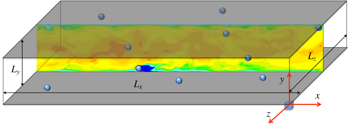
Sketch of a turbulent channel flow with a few fixed particles.

We consider the wall-bounded turbulent flow in a channel. As shown in figure 1, the flow between two infinite flat plates is driven by a constant body force  $g$ per unit mass. Spatial coordinates
 $x$,
 $y$ and
 $z$ represent the streamwise, transverse and spanwise direction, respectively. The separation distance between the two plates is
 $L_{y}=2H$, where
 $H$ is the half-channel width. The streamwise and spanwise lengths of the channel are
 $L_{x}=12H$ and
 $L_{z}=4H$, respectively. When particles are absent, the balance between the total driving force and the viscous drag on the channel walls yields
 $L_{x}L_{y}L_{z}\unicode[STIX]{x1D70C}g=2L_{x}L_{z}\overline{\unicode[STIX]{x1D70F}_{w}}$, where
 $\unicode[STIX]{x1D70C}$ is the fluid density,
 $\overline{\unicode[STIX]{x1D70F}_{w}}$ is the time-averaged wall shear stress. The Reynolds number based on the friction velocity
 $Re_{\unicode[STIX]{x1D70F}}=u_{\unicode[STIX]{x1D70F}}H/\unicode[STIX]{x1D708}$ is set at
 $180$, where
 $u_{\unicode[STIX]{x1D70F}}=\sqrt{\overline{\unicode[STIX]{x1D70F}_{w}}/\unicode[STIX]{x1D70C}}$ is the friction velocity,
 $\unicode[STIX]{x1D708}$ is the kinematic viscosity of the fluid. Periodic boundary conditions are assumed in the streamwise and spanwise directions. On the wall surfaces, the no-slip condition is applied.
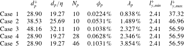
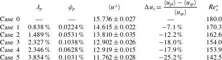
Key parameters used in the simulations. Parameters from the second to the last column are as follows: particle size in wall unit, particle size scaled by the Kolmogorov length at the wall, the number of particles, total particle volume fraction, total particle surface fraction, the smallest possible distance from a particle surface to closest channel wall, the largest possible distance from a particle surface to the closest channel wall.

As sketched in figure 1, a few spherical particles are placed at fixed locations in the channel to modify the background flow field. The diameter and the number of particles are varied in different cases, as shown in table 1. The background unladen flow is labelled as ‘Case 0’ to provide a contrast baseline to quantify the flow modulation. In all particle-laden cases, the particle volume fractions  $\unicode[STIX]{x1D719}_{p}=(N_{p}\unicode[STIX]{x03C0}d_{p}^{3}/6)/(L_{x}L_{y}L_{z})$ are kept very low (
 $\unicode[STIX]{x1D719}_{p}\ll 1\,\%$), where
 $N_{p}$ is the number of particles,
 $d_{p}$ is the diameter of particles. The first three particle-laden cases (Cases 1, 2 and 3) have the same number of particles but are different in the particle sizes. Case 3 and Case 4 have almost the same total particle surface areas (normalized by the channel wall area)
 $\unicode[STIX]{x1D706}_{p}=N_{p}\cdot \unicode[STIX]{x03C0}d_{p}^{2}/(2L_{x}L_{z})$, but different in particle volume fractions. Case 3 and Case 5 have almost the same
 $\unicode[STIX]{x1D719}_{p}$, but their total particle surface areas are different. In all five particle-laden cases, particles are placed close to the channel walls. This is because the most intensive flow modulation takes place near the wall, as reported in previous particle-laden turbulent wall-bounded flow studies (see Picano et al. Reference Picano, Breugem and Brandt2015; Wang et al. Reference Wang, Peng, Guo and Yu2016b; Peng & Wang Reference Peng and Wang2019). The near-wall turbulence is also the most inhomogeneous and anisotropic, thus the interplay of particle disturbance flows and the wall-generated turbulence is likely most intense and interesting. The wall-normal locations of the particle centres are only allowed to vary in a small range
 $(l_{y,min}+0.5d_{p},l_{y,max}-0.5d_{p})$, with
 $l_{y,min}$ equal to two grid lengths, to ensure that all the particles are placed close to the channel walls. Within this small range, particles are randomly distributed. In table 1, the values of
 $l_{y,min}$ and
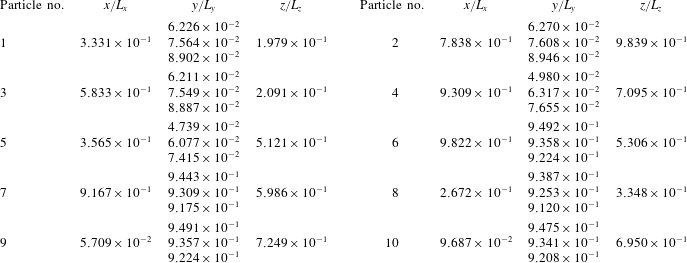
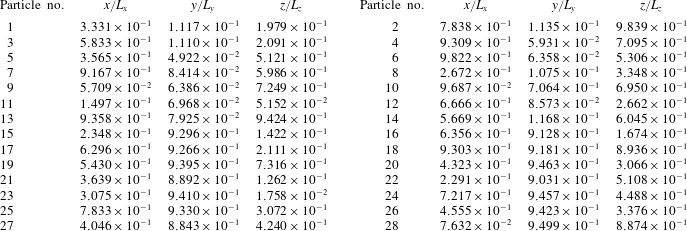
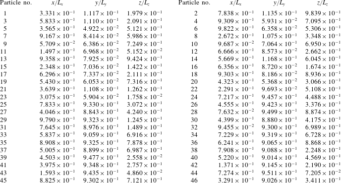
 $l_{y,max}$ in each particle-laden case are given. The locations of particles in each case are listed in tables 5–7 in appendix A. The streamwise and spanwise locations of the particle centres are also randomly chosen within the simulation domain of the channel. The driving force per unit fluid volume
 $\unicode[STIX]{x1D70C}g$ is kept constant for all simulation cases. In some other studies, such as Kulick et al. (Reference Kulick, Fessler and Eaton1994), Picano et al. (Reference Picano, Breugem and Brandt2015), Vreman & Kuerten (Reference Vreman and Kuerten2018), the driving force was tuned to maintain the same mass flux in the single-phase and particle-laden cases. The difference in settings between these studies and the present study is emphasized here to ensure that caution is employed when comparing the results directly.
A uniform mesh in Cartesian coordinates is used for all the simulations, with an identical grid resolution of  $N_{x}\times N_{y}\times N_{z}=1800\times 299\times 600$. The grid resolution, normalized by the wall unit of the single-phase turbulent channel flow case under the chosen
 $Re_{\unicode[STIX]{x1D70F}}=180$ is equal to
 $\unicode[STIX]{x1D6FF}_{x}^{+}=\unicode[STIX]{x1D6FF}_{y}^{+}=\unicode[STIX]{x1D6FF}_{z}^{+}=1.204$. The superscript
 $+$ indicates that a quantity has been normalized by the wall unit
 $y_{\unicode[STIX]{x1D70F}}=\unicode[STIX]{x1D708}/u_{\unicode[STIX]{x1D70F}}$ and the friction velocity
 $u_{\unicode[STIX]{x1D70F}}$. The choice of this resolution is based on two considerations. First, published DNS datasets (see, e.g. Kim, Moin & Moser (Reference Kim, Moin and Moser1987) and Moser, Kim & Mansour (Reference Moser, Kim and Mansour1999)) in a single-phase turbulent channel flow have shown that the maximum local dissipation rate near the channel wall has a value of
 $\unicode[STIX]{x1D716}^{+}\approx 0.16$, which results in a local Kolmogorov length scale of
 $\unicode[STIX]{x1D702}^{+}\approx 1.5$ on the wall. The grid resolution in the present simulations is chosen to be smaller than the size of this minimum flow length scale, which is sufficient to resolve the smallest eddy structures in the near-wall regions. Second, the grid resolution in the simulations should be set to resolve the boundary layer on the particle surfaces. The boundary layer thickness around a particle can be estimated as
 $\unicode[STIX]{x1D6FF}\approx d_{p}/\sqrt{Re_{p}}$, where
 $Re_{p}$ is the particle Reynolds number (see Xu & Subramaniam Reference Xu and Subramaniam2010). In the present particle-laden simulations, the range of particle Reynolds number is approximately 100–300, which makes the boundary layer thickness
 $1.386\unicode[STIX]{x1D6FF}_{x}$ to
 $2.4\unicode[STIX]{x1D6FF}_{x}$. The grid resolution
 $\unicode[STIX]{x1D6FF}_{x,y,z}^{+}=1.204$ ensures there is at least one point inside the boundary layer around the particles. It is worth mentioning that Xu & Subramaniam (Reference Xu and Subramaniam2010) suggested two points were necessary to resolve a boundary layer around a particle for the immersed boundary method. However, it is reasonable to relax this criterion for the boundary treatment scheme used in the present simulations, which has a second-order accuracy (see Peng, Ayala & Wang Reference Peng, Ayala and Wang2019a). A validation test will be given in § 3 for the case of a uniform flow passing a fixed particle to justify this point.
2.2 The lattice Boltzmann method
The lattice Boltzmann method is used for the fluid flow simulation in this study. Unlike the conventional computational fluid dynamics (CFD) methods that solve the discretized NS equations, LBM solves the evolution of the particle distribution functions (known as lattice Boltzmann equation (LBE)) of a few selected discrete particle velocities. The continuity and the NS equations can be derived as the zeroth- and first-order moment equations of LBE (Peng, Guo & Wang Reference Peng, Guo and Wang2017). The pressure and velocity are also directly obtained from the molecular distribution functions by taking moments. Therefore, it is no longer necessary to solve the Poisson equation for the pressure field in LBM. Following our previous studies (Gao et al. Reference Gao, Li and Wang2013; Wang et al. Reference Wang, Peng, Guo and Yu2016b), the multiple-relaxation time (MRT) LBE is selected for its better numerical stability over the single-relaxation time (SRT) LBE (see, e.g., d’Humières et al. (Reference d’Humières, Ginzburg, Krafczyk, Lallemand and Luo2002)). The evolution equation of the particle distribution functions in a MRT-LBM reads
 $$\begin{eqnarray}\boldsymbol{f}(\boldsymbol{x}+\boldsymbol{e}_{\unicode[STIX]{x1D6FC}}\unicode[STIX]{x1D6FF}_{t},t+\unicode[STIX]{x1D6FF}_{t})-\boldsymbol{f}(\boldsymbol{x},t)=-\unicode[STIX]{x1D648}^{-1}\unicode[STIX]{x1D64E}[\boldsymbol{m}(\boldsymbol{x},t)-\boldsymbol{m}^{(eq)}(\boldsymbol{x},t)]+\unicode[STIX]{x1D648}^{-1}\unicode[STIX]{x1D733},\end{eqnarray}$$
where  $\boldsymbol{f}$ is the vector of distribution functions,
 $\boldsymbol{e}_{\unicode[STIX]{x1D6FC}}$ are the selected discrete velocities,
 $\boldsymbol{x}$ and
 $t$ are the spatial and time coordinates, respectively,
 $\unicode[STIX]{x1D6FF}_{t}$ is the lattice time step,
 $\unicode[STIX]{x1D648}$ is the transform matrix that relates the distribution function vector
 $\boldsymbol{f}$ to a moment vector
 $\boldsymbol{m}$ with the same vector length;
 $\boldsymbol{m}^{(eq)}$ is the equilibrium part of
 $\boldsymbol{m}$;
 $\unicode[STIX]{x1D64E}$ is a diagonal matrix of the relaxation parameters. In MRT-LBE, the collision is treated in the moment space, where each moment could be assigned an individual relaxation parameter. The better numerical stability in MRT-LBM over its SRT counterpart can be achieved via optimizing the relaxation parameters of the moments that are irrelevant to the NS equations. It should be emphasized that adjusting these irrelevant relaxation parameters would not affect the physical NS solved by LBM and the order of discretization error, although they may affect the numerical stability and the magnitude of the numerical errors. The term
 $\unicode[STIX]{x1D733}$ is the vector of mesoscopic forcing terms. The body force in the NS equations is realized through this term.
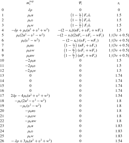
Unlike most of the previous LBM studies on particle-laden turbulent flow simulations (Ten Cate et al. Reference Ten Cate, Derksen, Portela and Van Den Akker2004; Gao et al. Reference Gao, Li and Wang2013; Wang et al. Reference Wang, Peng, Guo and Yu2016b; Eshghinejadfard et al. Reference Eshghinejadfard, Abdelsamie, Hosseini and Thévenin2017) where a D3Q19 (three-dimensional grid with nineteen discrete velocities) lattice model was used, a D3Q27 (three-dimensional grid with twenty-seven discrete velocities) lattice model is chosen here. This change is made in light of our recent finding that simulations based on a D3Q27 lattice tend to provide better numerical stability when the flow Reynolds number is relatively high (Peng & Wang Reference Peng and Wang2019). The definitions of the equilibrium moments  $\boldsymbol{m}^{(eq)}$, the mesoscopic forcing terms
 $\unicode[STIX]{x1D733}$ and the relaxation parameters
 $\unicode[STIX]{x1D64E}$ in the present D3Q27 MRT-LBM model are compiled in table 8 in appendix B. Compared to its counterpart based on the D3Q19 lattice, a simulation with the D3Q27 lattice has an approximately
 $(27-19)/19=42\,\%$ computational overhead, which is affordable.
At the end of each time step, the hydrodynamic variables, including the local density fluctuation  $\unicode[STIX]{x1D6FF}\unicode[STIX]{x1D70C}$, pressure
 $p$ and momentum
 $\unicode[STIX]{x1D70C}_{0}\boldsymbol{u}$, are computed directly from the distribution functions as
 $$\begin{eqnarray}\unicode[STIX]{x1D6FF}\unicode[STIX]{x1D70C}=\mathop{\sum }_{\unicode[STIX]{x1D6FC}=0}^{26}f_{\unicode[STIX]{x1D6FC}},\quad p=c_{s}^{2}\unicode[STIX]{x1D6FF}\unicode[STIX]{x1D70C},\quad \unicode[STIX]{x1D70C}_{0}\boldsymbol{u}=\mathop{\sum }_{\unicode[STIX]{x1D6FC}=0}^{26}f_{\unicode[STIX]{x1D6FC}}\boldsymbol{e}_{\unicode[STIX]{x1D6FC}}+\frac{\boldsymbol{F}\unicode[STIX]{x1D6FF}_{t}}{2},\end{eqnarray}$$
where the speed of sound  $c_{s}$ is equal to
 $1/\sqrt{3}$.
There are two categories of no-slip boundary treatments in LBM. One category is the immersed boundary lattice Boltzmann method (IB-LBM). The IB-LBM is generally similar to the immersed boundary method (IBM) in conventional CFD methods in that the velocity constraint on a no-slip boundary is converted to a body force applied locally to the fluid node points adjacent to the fluid–solid interfaces (Feng & Michaelides Reference Feng and Michaelides2005; Wu & Shu Reference Wu and Shu2009). The other category is the bounce-back schemes where the no-slip boundary is realized by directly constructing the missing distribution functions at the boundary grid points (see, e.g., Bouzidi, Firdaouss & Lallemand (Reference Bouzidi, Firdaouss and Lallemand2001)). The local interactions between the fluid and solid phases are handled through the momentum exchange between the two phases carried by the lattice particles crossing the fluid–solid interfaces (Ladd Reference Ladd1994; Bouzidi et al. Reference Bouzidi, Firdaouss and Lallemand2001). In this study, the no-slip boundaries on the fixed particle surfaces are treated with the quadratic interpolated bounce-back scheme by Bouzidi et al. (Reference Bouzidi, Firdaouss and Lallemand2001). This scheme ensures a second-order accurate velocity field that may not be achievable in IB-LBM. The hydrodynamic interaction between the fluid and particles is calculated via a momentum exchange scheme (Ladd Reference Ladd1994), which sums up the changes of momenta of all the lattice particles involved in the bounce-back interactions with a solid surface. In order to avoid a strong perturbation resulting from the velocity discontinuity around fixed particles, particles are inserted in the flow field as small seeds, whose diameter increases gradually until they reach the final particle size. The same strategy is adopted in the validation test of a uniform flow passing a fixed spherical particle. In this study, we only focus on investigating the statistics at the statistically stationary state, which should not be affected by how the flow is initialized. This principle has been often taken advantage of to design a better way to perturb flow and accelerate turbulent transition in wall-bounded turbulent flow simulations (see e.g. Pringle, Willis & Kerswell (Reference Pringle, Willis and Kerswell2012) and Rabin, Caulfield & Kerswell (Reference Rabin, Caulfield and Kerswell2012)). Strategies for releasing particles gradually are also not uncommon in particulate flow simulations. In the very first PR-DNS by Pan & Banerjee (Reference Pan and Banerjee1997), particles were inserted by gradually adapting the fluid velocity in the region occupied by particles to rigid-body motions. That work used a spectral method to solve the flow and an immersed boundary method to treat the particle surface.
3 Validation of the simulation codes
The simulation code in the present study is first validated in two benchmark cases: a uniform flow passing a fixed sphere and a single-phase turbulent channel flow.
3.1 A uniform stream passing a fixed sphere
The first case considered here is the classic flow of a uniform flow passing a fixed sphere in an unbounded domain. A spherical particle is fixed at  $(x_{c},y_{c},z_{c})=(6.25d_{p},6.25d_{p},6.25d_{p})$ in a cuboid domain of a size
 $(L_{x},L_{y},L_{z})=(25d_{p},12.5d_{p},12.5d_{p})$, where
 $d_{p}$ is the particle diameter. A uniform flow
 $\boldsymbol{u}=(u_{x},u_{y},u_{z})=(U_{in},0,0)$ enters the inlet of the domain, i.e.
 $x=0$, and passes over the fixed particle. The four rectangular sides are set to be stress-free i.e.
 $u_{z}=0,\unicode[STIX]{x2202}u_{x}/\unicode[STIX]{x2202}z=\unicode[STIX]{x2202}u_{y}/\unicode[STIX]{x2202}z=0$ at
 $z=0$ and
 $z=L_{z}$, and
 $u_{y}=0,\unicode[STIX]{x2202}u_{x}/\unicode[STIX]{x2202}y=\unicode[STIX]{x2202}u_{z}/\unicode[STIX]{x2202}y=0$ at
 $y=0$ and
 $y=L_{y}$, to mimic the boundary condition in an infinite domain. The flow exits the domain with an outflow boundary condition
 $\unicode[STIX]{x2202}(\unicode[STIX]{x1D70C}_{0}\boldsymbol{u})/\unicode[STIX]{x2202}t+U_{out}\unicode[STIX]{x2202}(\unicode[STIX]{x1D70C}_{0}\boldsymbol{u})/\unicode[STIX]{x2202}x=0$, where
 $U_{out}$ is the local streamwise velocity at the outlet. The outflow boundary is implemented in terms of distribution functions as
 $f_{i}(L_{x},t+\unicode[STIX]{x1D6FF}_{t})=[f_{i}(L_{x},t)+\unicode[STIX]{x1D706}f_{i}(L_{x}-\unicode[STIX]{x1D6FF}_{x},t+\unicode[STIX]{x1D6FF}_{t})]/(1+\unicode[STIX]{x1D706})$, where
 $\unicode[STIX]{x1D706}=U_{out}\unicode[STIX]{x1D6FF}_{t}/\unicode[STIX]{x1D6FF}_{x}$ (Lou, Guo & Shi Reference Lou, Guo and Shi2013).
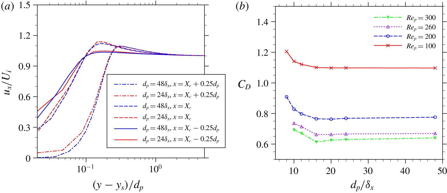
At a particle Reynolds number  $Re_{p}=U_{in}d_{p}/\unicode[STIX]{x1D708}=260$, fluid velocity profiles on three selected lines,
 $(x,z)=(x_{c}-0.25d_{p},z_{c})$,
 $(x_{c},z_{c})$,
 $(x_{c}+0.25d_{p},z_{c})$ crossing the front edge, centre and trailing edge of the particle are shown as functions of distance from the particle surface in figure 2(a), with two different grid resolutions
 $d_{p}=24\unicode[STIX]{x1D6FF}_{x}$ and
 $d_{p}=48\unicode[STIX]{x1D6FF}_{x}$. The particle Reynolds number
 $Re_{p}=260$ is chosen because it is close to the up limit
 $Re_{p}=270$, above which an unsteady wake after the particles would form (see Jones & Clarke Reference Jones and Clarke2008), and it is representative to the particle Reynolds number encountered in the particle-laden turbulent flow simulation in this study. While there are certain deviations very close to the particle surface, the fluid velocities with the grid resolution
 $d_{p}=24\unicode[STIX]{x1D6FF}_{x}$ generally match well with the results obtained from the higher grid resolution
 $d_{p}=48\unicode[STIX]{x1D6FF}_{x}$. The drag coefficient measured in the two cases are 0.6661 and 0.6696, which is an approximately 0.52 % difference. In addition, the measured drag coefficients of the particle at
 $Re_{p}=100$,
 $200$, and
 $300$ as functions of grid resolutions are shown in figure 2(b). The maximum deviation of the drag coefficient measured with the grid resolution
 $d_{p}=24\unicode[STIX]{x1D6FF}_{x}$ with respect to the results measured with the doubled grid resolution
 $d_{p}=48\unicode[STIX]{x1D6FF}_{x}$ is 1.68 % at
 $Re_{p}=300$. Grid mesh independence is roughly obtained with
 $d_{p}=24\unicode[STIX]{x1D6FF}_{x}$ for all four Reynolds numbers. From these results we can conclude that, although a grid resolution
 $d_{p}=24\unicode[STIX]{x1D6FF}_{x}$ may not be sufficient to fully resolve the local flow around particles, for the purpose of studying the averaged flow statistics, this grid resolution should be adequate.
Simulated (a) profiles of local flow velocity, and (b) drag coefficients in a uniform flow passing a fixed sphere.

3.2 A single-phase turbulent channel flow (Case 0)
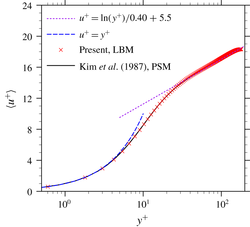
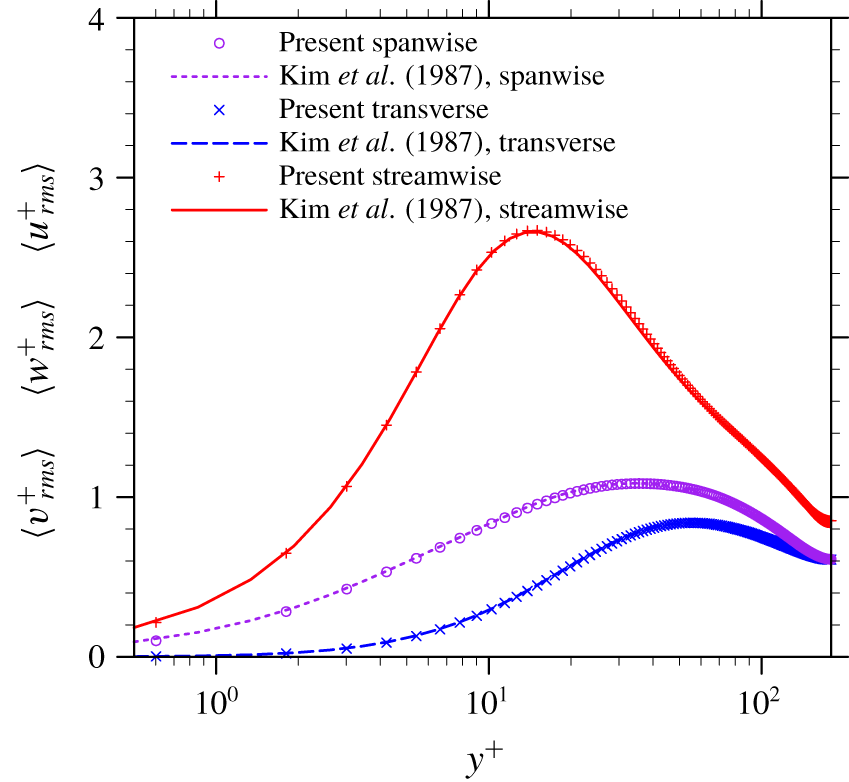
The fully developed single-phase channel flow is investigated to validate the flow simulation part of the code and to provide a fully developed background flow field to initialize the particle-laden flow simulations. Details on the flow initialization and fast transition to the developed flow can be found in Wang et al. (Reference Wang, Peng, Guo and Yu2016b). Once the flow reaches its statistical stationary state, the turbulent statistics are calculated. The turbulent statistics are averaged in the two homogeneous directions, i.e. streamwise and spanwise directions, and over approximately 30 eddy turnover times (the eddy turnover time is defined as  $H/u_{\unicode[STIX]{x1D70F}}$). The statistics of the mean flow velocity
 $\overline{\langle u^{+}\rangle }$ and the root-mean-square (r.m.s.) velocities (
 $\overline{\langle u_{rms}^{+}\rangle }$,
 $\overline{\langle v_{rms}^{+}\rangle }$ and
 $\overline{\langle w_{rms}^{+}\rangle }$) are shown in figures 3 and 4, respectively. Here, the notation
 $\langle \cdots \rangle$ indicates the phase averaging, and
 $\overline{\cdots \,}$ indicates the time averaging. Both the mean and fluctuation velocities are in excellent agreement with the benchmark results from a Chebyshev pseudo-spectral simulation by Kim et al. (Reference Kim, Moin and Moser1987), even in the region near the wall.
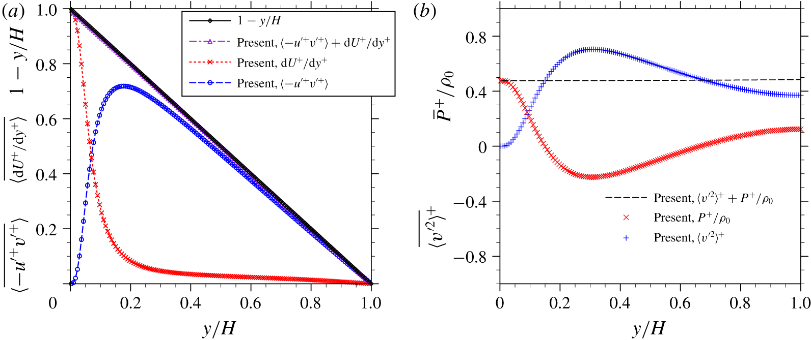
In a turbulent channel flow, it can be shown that the stress balances in the streamwise ( $x$) and transverse (
 $y$) directions at the statistically stationary state are
 $$\begin{eqnarray}\displaystyle & \displaystyle \overline{\langle -u^{\prime +}v^{\prime +}\rangle }+\frac{\text{d}\overline{\langle u\rangle }^{+}}{\text{d}y^{+}}=1-\frac{y}{H} & \displaystyle\end{eqnarray}$$
 $$\begin{eqnarray}\displaystyle & \displaystyle \overline{\langle v^{\prime 2}\rangle ^{+}}+\frac{\overline{\langle p\rangle ^{+}}}{\unicode[STIX]{x1D70C}_{0}}=\text{const.}, & \displaystyle\end{eqnarray}$$
 $p$ is the pressure,
 $\unicode[STIX]{x1D70C}_{0}$ is the fluid density. These two balance equations are examined in figure 5. The straight line in each plot confirms that the momentum balances in both the streamwise and transverse directions are well captured. Such results also imply that quantities in (3.1) are averaged for a sufficiently long time (30 eddy turnover times) so they are no longer average-time-duration dependent.
Mean flow velocity profiles in a single-phase turbulent channel flow.

Root-mean-square velocity profiles in a single-phase turbulent channel flow.

Streamwise (a) and transverse (b) momentum balance in a single-phase turbulent channel flow at statistically stationary state.

4 Turbulent channel flows laden with a few fixed particles
In this section, the simulation results of turbulent channel flows laden with fixed particles are presented and discussed. The five particle-laden cases start from the same background flow (i.e. the fully developed single-phase turbulent channel flow, Case 0). Particles are inserted in the background flow initially as small seeds and then grow gradually to their final sizes. The whole insertion process took approximately 1 eddy turnover time and the new stationary states were established gradually after approximately 25 eddy turnover times after the particle insertion. Unless specifically stated, results discussed in this section are still normalized by the length, time and velocity scales in the single-phase turbulent channel flow case. These statistics are also by default phase averaged over the region occupied by the fluid, and time averaged over 30 eddy turnover times.
4.1 Modulation of the bulk flow velocity by particles
4.1.1 General observations
The simulated bulk flow velocity in different cases.

At the stationary state, the bulk flow velocity magnitudes averaged over the whole fluid domain in each case are listed in table 2. The mean flow velocities are reduced in all five particle-laden cases compared to the single-phase case. In particular, Case 3 and Case 4, with roughly the same particle total surface area but different particle volume fractions, have comparable mean flow velocities. This indicates the mean flow velocity reduction roughly scales with the total particle surface area instead of the particle volume fraction. Cisse et al. (Reference Cisse, Saw, Gibert, Bodenschatz and Bec2015) reported a similar observation in their experiments that the turbulence attenuation in a von Kármán flow scales with  $\unicode[STIX]{x1D719}_{p}^{2/3}$ when the particle volume fraction
 $\unicode[STIX]{x1D719}_{p}$ is small. It is well known that the drag force on a single particle in an undisturbed flow scales roughly with
 $d_{p}^{2}$ (or the projected surface area
 $A=\unicode[STIX]{x03C0}d_{p}^{2}/4$) if the particle Reynolds number is of the order of 1000, i.e.
 $F_{D}=C_{D}\unicode[STIX]{x1D70C}u^{2}A/2$, where
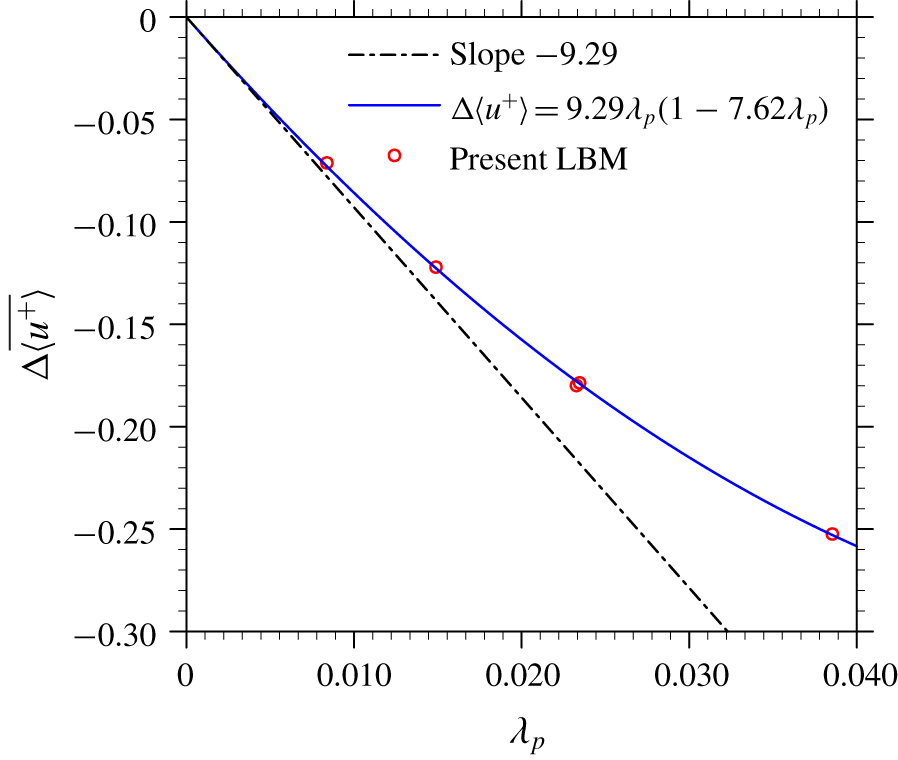
 $C_{D}$ is the drag coefficient. In our simulations, the particle Reynolds number is estimated to be in the range of 100–300. The total drag force from the particles may also scale roughly with the total particle surface area. From Case 1 to Case 5, the reduction of the mean flow velocity increases with the total particle surface area, but with a decreasing slope. This decreasing slope implies that the inter-particle interactions start to play a more important role when particle volume fraction increases. A simple argument to make is that, when a solid particle is in the wake region of another solid particle, it shall experience a smaller resistance to the flow than the scenario in which the particle is exposed in an undisturbed flow. The wake region created behind a single particle also scales with its cross-sectional area. Considering the low particle volume fractions, the total area of the wake region should also be proportional to the total particle surface area. The relative reduction of the bulk flow velocity is thus correlated with the total particle surface area
 $\unicode[STIX]{x1D706}_{p}$ as
 $$\begin{eqnarray}\unicode[STIX]{x0394}u_{x}=(1-C_{1}\unicode[STIX]{x1D706}_{p})C_{2}\unicode[STIX]{x1D706}_{p}.\end{eqnarray}$$
The results in the present simulations fit well to a curve with  $C_{1}=7.62$,
 $C_{2}=-9.29$, as shown in figure 6.
Relative reduction of bulk flow speed as a function of total particle surface area.

Mean velocity profiles in single-phase and particle-laden turbulent channel flow simulations.

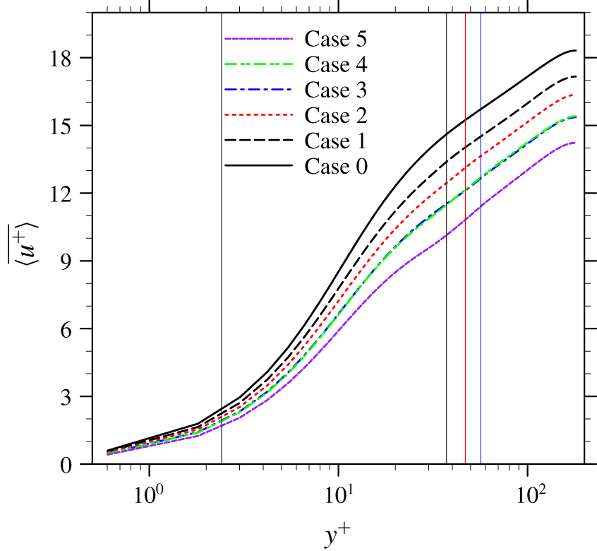
The profiles of the mean flow velocity  $\langle u^{+}\rangle$ in each simulation are presented in figure 7. The upper bound
 $l_{y,max}^{+}$ and lower bound
 $l_{y,min}^{+}$ of the region that is directly altered by particles are marked by the straight vertical lines in figure 7. The five particle-laden flow cases share the same lower bound but have three different upper bounds, as shown in table 1. As presented in figure 7, the mean flow velocity is directly altered by the presence of particles in the region below
 $l_{y,max}$. The reduction of the mean flow velocity propagates outside
 $l_{y,max}$, and causes shifted mean velocity profiles in the log-law region. The slope of the mean velocity profiles in the log-law region are, however, almost unchanged. This observation is in contrast with these reported in other IR-DNS studies of particle-laden turbulent channel flow with moving particles, (Picano et al. Reference Picano, Breugem and Brandt2015; Wang et al. Reference Wang, Peng, Guo and Yu2016a; Eshghinejadfard et al. Reference Eshghinejadfard, Abdelsamie, Hosseini and Thévenin2017) where the effective von Kármán constants were reported smaller than the unladen case, i.e. the slopes in the log-law region were steeper.
4.1.2 An analysis of the stress balance equation
To better understand the modifications of the mean velocity profiles, the volume-averaged stress balance equation in the fluid phase is investigated. In a particle-laden turbulent channel flow, the average streamwise momentum balance at the stationary stage can be written as
 $$\begin{eqnarray}\underbrace{\overline{\unicode[STIX]{x1D6FC}\langle -u^{\prime }v^{\prime }\rangle }}_{\unicode[STIX]{x1D70F}_{R}}+\underbrace{\frac{1}{\unicode[STIX]{x1D70C}}\overline{\unicode[STIX]{x1D6FC}\unicode[STIX]{x1D707}\left\langle \frac{\unicode[STIX]{x2202}u}{\unicode[STIX]{x2202}y}\right\rangle }}_{\unicode[STIX]{x1D70F}_{V}}+\underbrace{\frac{1}{\unicode[STIX]{x1D70C}V}\int _{0}^{y}\overline{F_{x}}\,\text{d}y}_{\unicode[STIX]{x1D70F}_{P}}=\underbrace{\frac{\overline{\unicode[STIX]{x1D70F}_{w,pl}}}{\unicode[STIX]{x1D70C}}-g\int _{0}^{y}\overline{\unicode[STIX]{x1D6FC}}\,\text{d}y}_{\unicode[STIX]{x1D70F}_{T}},\end{eqnarray}$$
where  $\unicode[STIX]{x1D6FC}$ is the average volume fraction of the fluid phase inside the control volume
 $V$. Here, we define
 $V$ as a thin slab stretching in the two homogeneous directions, i.e.
 $x$ and
 $z$,
 $V=L_{x}L_{z}\unicode[STIX]{x1D6FF}_{y}$.
 $F_{x}=\int _{S_{I}\in V}n_{j}\unicode[STIX]{x1D70E}_{xj}\,\text{d}S$ is the total hydrodynamic force in the streamwise direction exerted on the fluid phase by the solid surfaces present in
 $V$;
 $\overline{\unicode[STIX]{x1D70F}_{w,pl}}$ is the counterpart of mean wall stress
 $\overline{\unicode[STIX]{x1D70F}_{w}}$ in particle-laden cases, whose value can be obtained by replacing the integration limit
 $y$ with the half-channel width
 $H$ in (4.2) as
 $$\begin{eqnarray}\overline{\unicode[STIX]{x1D70F}_{w,pl}}=\unicode[STIX]{x1D70C}gH\unicode[STIX]{x1D719}_{f}+\frac{1}{V}\int _{0}^{H}\overline{F_{x}}\,\text{d}y.\end{eqnarray}$$
The four terms in (4.2) represent the Reynolds stress, viscous stress, particle-interface stress and the total stress, respectively, and they are given the shorthand notations  $\unicode[STIX]{x1D70F}_{R}$,
 $\unicode[STIX]{x1D70F}_{V}$,
 $\unicode[STIX]{x1D70F}_{P}$ and
 $\unicode[STIX]{x1D70F}_{T}$, respectively. This equation can be derived via the theorem of volume averaging (see Prosperetti & Tryggvason Reference Prosperetti and Tryggvason2009; Crowe et al. Reference Crowe, Schwarzkopf, Sommerfeld and Tsuji2011) or the phase-field theorem (see Kataoka & Serizawa Reference Kataoka and Serizawa1989; Vreman & Kuerten Reference Vreman and Kuerten2018).
A similar stress balance equation was derived by Picano et al. (Reference Picano, Breugem and Brandt2015) and Yu et al. (Reference Yu, Lin, Shao and Wang2017) in a particle-laden turbulent channel flow. This stress balance equation is written as
 $$\begin{eqnarray}\underbrace{\overline{\unicode[STIX]{x1D6FC}\langle -u^{\prime }v^{\prime }\rangle }}_{\unicode[STIX]{x1D70F}_{R}}+\underbrace{\overline{(1-\unicode[STIX]{x1D6FC})\langle -u^{\prime }v^{\prime }\rangle _{p}}}_{\unicode[STIX]{x1D70F}_{R,p}}+\underbrace{\frac{1}{\unicode[STIX]{x1D70C}}\overline{\unicode[STIX]{x1D6FC}\unicode[STIX]{x1D707}\left\langle \frac{\unicode[STIX]{x2202}u}{\unicode[STIX]{x2202}y}\right\rangle }}_{\unicode[STIX]{x1D70F}_{V}}+\underbrace{\frac{1}{\unicode[STIX]{x1D70C}}\overline{(1-\unicode[STIX]{x1D6FC})\langle \unicode[STIX]{x1D70E}_{xy}\rangle _{p}}}_{\unicode[STIX]{x1D70F}_{I}}=\underbrace{u_{\unicode[STIX]{x1D70F}}^{2}-gy}_{\unicode[STIX]{x1D70F}_{T,m}},\end{eqnarray}$$
where  $\unicode[STIX]{x1D70F}_{R,p}$ is the particle Reynolds stress,
 $\unicode[STIX]{x1D70F}_{I}$ is the particle inner stress and
 $\unicode[STIX]{x1D70F}_{T,m}$ is the total stress for the fluid–particle mixture. It is worth mentioning that (4.4) is applied to the fluid–particle mixture, so the explicit computation of the
 $\unicode[STIX]{x1D70F}_{P}$ in (4.2) is no longer necessary. As a trade-off, counterparts of the Reynolds stress
 $\unicode[STIX]{x1D70F}_{R}$ and the viscous stress
 $\unicode[STIX]{x1D70F}_{V}$ applied to the particle phase, i.e.
 $\unicode[STIX]{x1D70F}_{R,p}$ and
 $\unicode[STIX]{x1D70F}_{I}$, must be introduced into the stress balance equation. In particular, the particle inner stress term has no clear physical meaning and cannot be evaluated explicitly. On the other hand, each term in (4.2) can be explicitly computed using the DNS data.
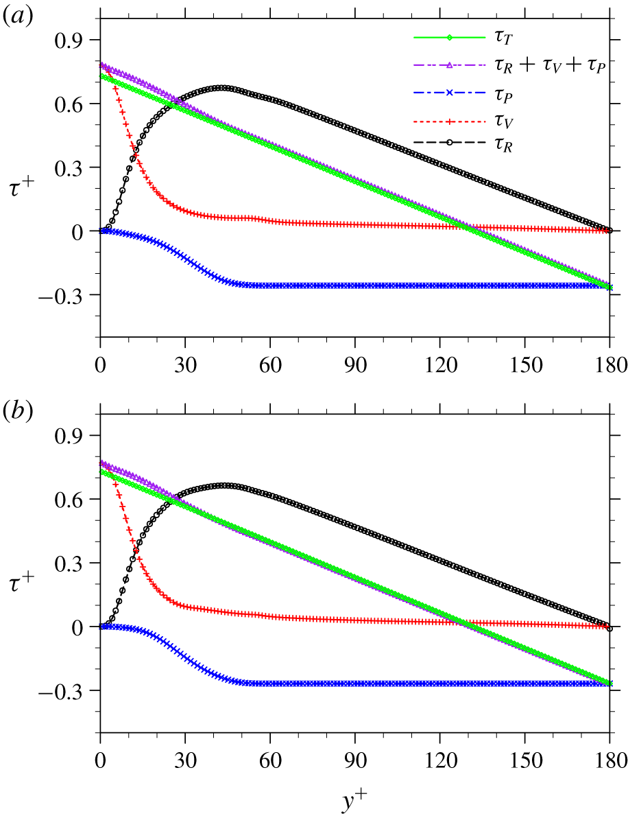
Stress balance in a particle-laden turbulent channel flow: (a) Case 3, (b) Case 4.

Equation (4.2) is examined in each particle-laden flow case in figure 8. For conciseness, only the results in Case 3 and Case 4 are shown. Note that  $\langle \unicode[STIX]{x2202}u_{x}/\unicode[STIX]{x2202}y\rangle$ and
 $\unicode[STIX]{x2202}\langle u_{x}\rangle /\unicode[STIX]{x2202}y$ are identical when the fluid volume fraction
 $\unicode[STIX]{x1D6FC}$ is constant over time, which applies to the present simulations where particles are fixed. (According to the Leibniz integral rule (or the Reynolds transport theorem), when the total amount of the fluid is changing in
 $V$, the derivative of a phase-averaged fluid velocity is different from the phase average of the velocity derivative.) The balance in (4.2) is well captured by the DNS data, as the purple line representing the left-hand side of the equation collapses with the green line representing the right-hand side in most parts of the channel in each case, except in a region close to the wall. The maximum deviation from the balance
 $\unicode[STIX]{x1D70F}_{R}+\unicode[STIX]{x1D70F}_{V}+\unicode[STIX]{x1D70F}_{P}=\unicode[STIX]{x1D70F}_{T}$ is observed near the channel wall in Case 5, which is approximately
 $0.05\unicode[STIX]{x1D70C}gH$. This deviation is likely due to the numerical error of computing the velocity gradient term near the channel wall. When particles are present, there are only two layers of grid points between the particles and the channel wall, which may not be sufficient to fully resolve the flow in the gaps locally.
Since particles only locate in a certain wall-normal range between  $l_{y,min}^{+}$ and
 $l_{y,max}^{+}$, flows are expected to be distinct in the particle-laden region of
 $l_{y,min}^{+}\leqslant y^{+}\leqslant l_{y,max}^{+}$, and the outer region of
 $y^{+}-l_{y,max}^{+}\gg 1$. In the outer region, the whole volume is occupied by the fluid phase, so
 $\unicode[STIX]{x1D6FC}=1$. The stress balance equation, equation (4.2), can then be simplified as
 $$\begin{eqnarray}\overline{\langle -u^{\prime }v^{\prime }\rangle }+\frac{1}{\unicode[STIX]{x1D70C}}\overline{\unicode[STIX]{x1D707}\frac{\unicode[STIX]{x2202}\langle u\rangle }{\unicode[STIX]{x2202}y}}=(H-y)g.\end{eqnarray}$$
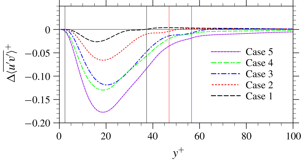
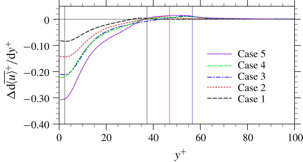
Note that (4.5) is identical to the stress balance equation in a single-phase turbulent channel flow. Both the Reynolds stress and the viscous stress in this outer region are therefore expected to be close to those in the single-phase case, as confirmed in figures 9 and 10. A same slope of the mean velocity profiles in the log-law region is observed.
Changes of Reynolds stress in particle-laden channel flow simulations compared to the single-phase case.

Changes of viscous stress in particle-laden channel flow simulations compared to the single-phase case.

In the region of  $y^{+}\leqslant l_{y,max}^{+}$, applying the same argument that the particle volume fraction is very low, i.e.
 $\unicode[STIX]{x1D6FC}\approx 1$, the stress balance equation (4.2) can be written as
 $$\begin{eqnarray}\overline{\langle -u^{\prime }v^{\prime }\rangle }+\frac{1}{\unicode[STIX]{x1D70C}}\overline{\unicode[STIX]{x1D707}\frac{\unicode[STIX]{x2202}\langle u\rangle }{\unicode[STIX]{x2202}y}}\approx (H-y)g+\frac{1}{V}\int _{y}^{H}\overline{F_{x}}\,\text{d}y.\end{eqnarray}$$
For the viscous sublayer, i.e.  $y\approx 0$, the viscous effect dominates, so the Reynolds stress can be removed for simplicity. The right-hand side of the equation is approximated as
 $Hg+1/V\int _{0}^{H}\overline{F_{x}}\,\text{d}y$, which is a constant in each particle-laden case. After normalization, equation (4.6) becomes
 $$\begin{eqnarray}\overline{\frac{\unicode[STIX]{x2202}\langle u\rangle ^{+}}{\unicode[STIX]{x2202}y^{+}}}\approx 1+\unicode[STIX]{x1D6FD},\end{eqnarray}$$
where  $\unicode[STIX]{x1D6FD}$ is a negative constant whose magnitude represents the percentage of particle-induced resistance in the total flow resistance. According to (4.7), the mean velocity profiles in the viscous sublayer in the particle-laden cases are still linear functions, but with smaller slopes. In each particle-laden case, an effective friction velocity can be defined as
 $$\begin{eqnarray}u_{\unicode[STIX]{x1D70F}}^{\ast }=u_{\unicode[STIX]{x1D70F}}\sqrt{1+\unicode[STIX]{x1D6FD}}.\end{eqnarray}$$
For Case 1 through Case 5, the effective friction velocities are calculated as  $(0.9462\pm 0.0053)u_{\unicode[STIX]{x1D70F}}$,
 $(0.9035\pm 0.0073)u_{\unicode[STIX]{x1D70F}}$,
 $(0.8555\pm 0.0105)u_{\unicode[STIX]{x1D70F}}$,
 $(0.8551\pm 0.0066)u_{\unicode[STIX]{x1D70F}}$,
 $(0.7917\pm 0.0103)u_{\unicode[STIX]{x1D70F}}$, respectively. The error terms represent the statistical uncertainty. The effective friction Reynolds number in each case calculated from the corresponding effective friction velocity is given in table 2. In all five particle-laden cases, the effective friction Reynolds numbers are reduced compared to the unladen case, which is opposite to the observation in some previous studies of turbulent channel flows with freely moving particles, e.g. Picano et al. (Reference Picano, Breugem and Brandt2015). As indicated by (4.3), at the statistically stationary state, the total driving force
 $\unicode[STIX]{x1D70C}gH\unicode[STIX]{x1D719}_{f}$ is balanced by the mean wall stress
 $\unicode[STIX]{x1D70F}_{w,pl}$ and the total particle drag
 $1/V\int _{0}^{H}\overline{F_{x}}\,\text{d}y$. Since the driving force per unit fluid volume is maintained constant in all cases and the particle volume fractions are small, the total driving force in each case is roughly unchanged. As particles provide an additional drag force to the fluid, the mean wall stress reduces, so does the effective friction Reynolds number. The fixed driving force in the present study is also responsible for the Reynolds stress reduction in the particle-laden cases (see figure 9). On the other hand, in those studies where enhanced effective friction Reynolds numbers relative to the unladen case were reported, driving forces were increased to maintain an unchanged mean fluid flux (see e.g. Picano et al. (Reference Picano, Breugem and Brandt2015)). This difference is once again emphasized to help readers digest the results reported in the present investigation.
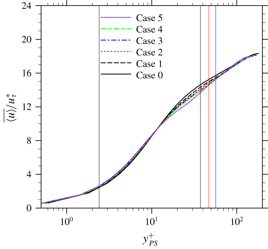
The mean velocity profiles shown in figure 7 normalized by the effective friction velocities in each case are shown in figure 11. The wall-normal locations are also normalized by the re-defined wall units based on the effective friction velocities (the kinematic viscosity  $\unicode[STIX]{x1D708}$ is viewed as a constant in different cases due to the fact that the particle volume fractions are small). In general, these mean velocity profiles more or less collapse with their counterpart in the single-phase case, but deviations are noted in the buffer region and log-law regions. These deviations are expected as the stress balance equations are quite distinct in the viscous sublayer (4.7) and the centre region (4.5) of the channel. Therefore, it is unlikely that the whole velocity profile in the particle-laden case can collapse with its single-phase counterpart using a single rescaling. It is worth mentioning that Costa et al. (Reference Costa, Picano, Brandt and Breugem2016) proposed a universal log law in particles-laden turbulent channel flows with dense particle suspensions. Their argument was made based on the observation that the local accumulation of particles near the channel walls could serve as a virtual wall and prevent direct interaction between the flows on the two sides of this virtual wall. In the present simulations, this universal log law does not apply, as the particle volume fractions are too smaller to form a virtual wall.
The profiles of the mean velocity rescaled by the effective friction velocities.

4.2 Modulation of the turbulence intensity by particles
4.2.1 General observations
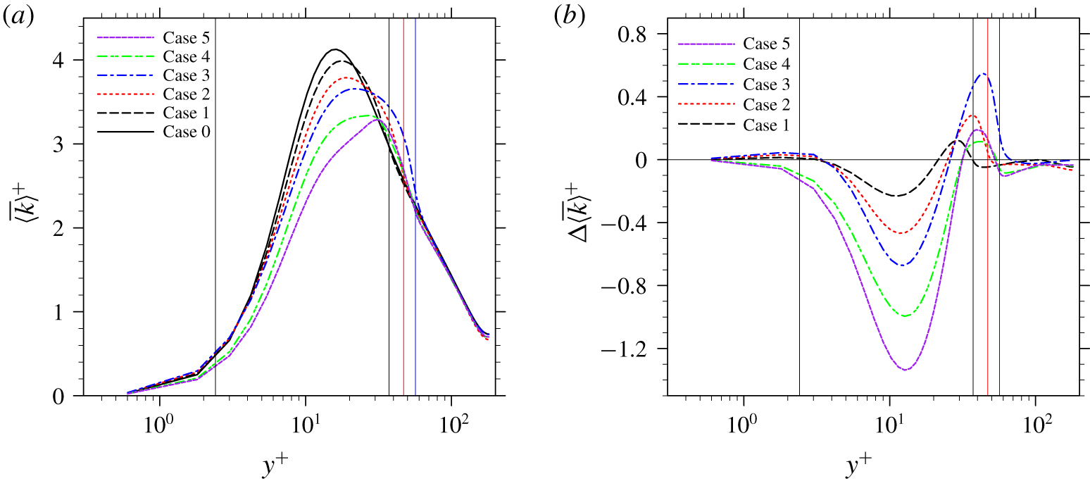
Turbulent kinetic energy profiles in single-phase and particle-laden turbulent channel flow simulations: (a) TKE profiles, (b) relative changes compared to the single-phase case.

Next, we consider the modulation of the turbulent intensity by particles. The profiles of the time-averaged turbulent kinetic energy  $\overline{\langle k\rangle ^{+}}=\frac{1}{2}\overline{\langle {u^{\prime }}^{2}+{v^{\prime }}^{2}+{w^{\prime }}^{2}\rangle ^{+}}$ from the single-phase and particle-laden flow cases are shown in figure 12. The distribution of TKE in the channel flow is significantly modified by the particles, and the modification is wall-normal location dependent. Around the peak of TKE distribution in the single-phase case, TKE is significantly reduced in all particle-laden cases. The same phenomenon was also observed in the particle-laden channel flow simulations with freely moving particles, as in Shao et al. (Reference Shao, Wu and Yu2012), Picano et al. (Reference Picano, Breugem and Brandt2015), Wang et al. (Reference Wang, Peng, Guo and Yu2016b) and Eshghinejadfard et al. (Reference Eshghinejadfard, Abdelsamie, Hosseini and Thévenin2017). This reduction, as shall be seen shortly, is associated with the reduction of the TKE production rate in the same region. Moving closer to the channel centre, TKE becomes augmented beyond the wall-normal location
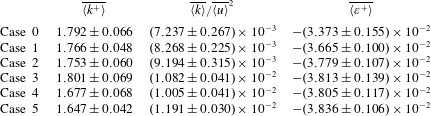
 $y^{+}\approx 25$. In the first three cases, the transition locations from TKE attenuation to TKE enhancement roughly correspond to the plane where the particle centres are located, in each case. In the last two cases, the transition locations move further towards the channel centre. The levels of enhancement in the last two cases are also much weaker than those in the first three cases. Near the channel centre, the presence of particles only slightly modifies the TKE. This is because particles are not present in this region. Because the modulation in this region is insignificant, it will not be discussed further. Using Simpson’s rule, the averaged TKE over the whole channel is calculated in each case. From Case 0 to Case 5, the values of the averaged TKE
 $\overline{\langle k^{+}\rangle }$ over the whole channel are given by the second column of table 3, all normalized by the friction velocity in the single-phase case. It is generally known from experimental observations that the nature of turbulence modification by solid particles depends on the particle size relative to the local integral scale of the turbulent flow (Gore & Crowe Reference Gore and Crowe1989). In the present simulations, the first three cases roughly exhibit the same turbulence intensity as that in the single-phase case, although the particle sizes are different. This implies that the relative particle size is not the only criterion to use to describe how the turbulence intensity is modified. A monotonic increase of turbulence intensity with the particle size is not observed in these three cases, probably due to the competing effects of increasing surface area and increasing particle size. On the other hand, a comparison of Case 3 and Case 4 under the same surface area does show that large TKE is associated with large particle size; and under the same volume fraction (Case 3 and Case 5), the average TKE also increases with the particle size. These are consistent with the general observation by Gore & Crowe (Reference Gore and Crowe1989). When the averaged TKE is normalized by the bulk flow velocity magnitude in each case, the results are presented by the third column in table 3. Therefore, in all five particle-laden cases, the turbulence intensities relative to the mean flow are enhanced by the present of the particles. Under this re-scaling, the turbulence intensity does increase with the particle size in the first three cases (Cases 1–3).
The simulated TKE and dissipation rates. The quantities behind  $\pm$ are the statistical uncertainties.

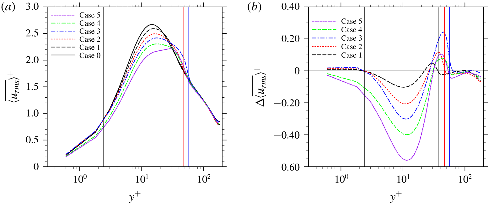
Streamwise r.m.s. velocity profiles in single-phase and particle-laden turbulent channel flow simulations: (a) streamwise r.m.s. velocity profiles, (b) relative changes compared to the single-phase case.

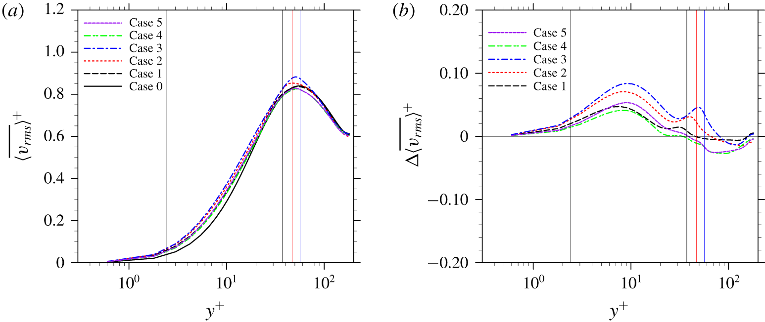
Wall-normal r.m.s. velocity profiles in single-phase and particle-laden turbulent channel flow simulations: (a) wall-normal r.m.s. velocity profiles, (b) relative changes compared to the single-phase case.

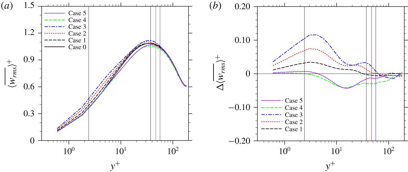
Spanwise r.m.s. velocity profiles in single-phase and particle-laden turbulent channel flow simulations: (a) spanwise r.m.s. velocity profiles, (b) relative changes compared to the single-phase case.

The profiles of the r.m.s. velocity in the streamwise, wall-normal and spanwise directions are presented in figures 13–15, respectively. The modulations are anisotropic for the different velocity components, consistent with the observations in previous particle-laden turbulent channel flow investigations (see Shao et al. Reference Shao, Wu and Yu2012; Picano et al. Reference Picano, Breugem and Brandt2015; Eshghinejadfard et al. Reference Eshghinejadfard, Abdelsamie, Hosseini and Thévenin2017). Among the three components, the modulation of the streamwise r.m.s. velocity is similar to that of the total TKE, which indicates a tight connection of the two. In the wall-normal direction, the r.m.s. velocity is enhanced in the region of  $y^{+}\leqslant l_{y,max}^{+}$, with an exception in the last two cases, where the wall-normal r.m.s. velocity is reduced in a small region around
 $l_{y,max}^{+}$. This difference, as will be clearer after the TKE budget analysis, is probably because the pressure transport is weaker in the last two cases due to smaller particle Reynolds numbers and a more scattered particle distribution in the wall-normal direction. This weaker pressure transport mechanism conveys smaller amounts of TKE from the bulk region towards to region around
 $y^{+}=l_{y,max}^{+}$. The modulations of the spanwise r.m.s. velocity are quite the opposite between the first three cases and the last two cases. In the first three cases, the spanwise r.m.s. velocities are enhanced in the region of
 $y^{+}\leqslant l_{y,max}^{+}$, which are similar to their counterparts of the wall-normal component, except that the maximum enhancements in the former occur within the viscous sublayer while in the latter the largest enhancements happen inside the buffer region. In the last two cases, however, the spanwise r.m.s. velocity is generally reduced through the whole channel, except in a small region attached to the channel walls where the spanwise r.m.s. velocities are slightly enhanced. This may be associated with the attenuated inter-component transfer of TKE from the other two components, as well as the enhanced dissipation rates of spanwise TKE, which will be discussed in detail in the next section.
4.2.2 Turbulent kinetic energy budget
To better understand the turbulence modulation due to the particles, a detailed TKE budget analysis is described next. The volume-averaged TKE budget equation of the fluid phase in any particle-laden flow with a control volume  $V$ can be derived as
 $$\begin{eqnarray}\displaystyle & & \displaystyle \frac{\unicode[STIX]{x2202}}{\unicode[STIX]{x2202}t}\unicode[STIX]{x1D6FC}\frac{1}{2}\langle u_{i}^{\prime }u_{i}^{\prime }\rangle =\underbrace{-\unicode[STIX]{x1D6FC}\langle u_{i}^{\prime }u_{j}^{\prime }\rangle \frac{\unicode[STIX]{x2202}\langle u_{i}\rangle }{\unicode[STIX]{x2202}x_{j}}}_{E_{P}}\underbrace{-\frac{\unicode[STIX]{x2202}}{\unicode[STIX]{x2202}x_{j}}\left[\unicode[STIX]{x1D6FC}\langle u_{j}\rangle \frac{1}{2}\langle u_{i}^{\prime }u_{i}^{\prime }\rangle \right]}_{E_{MT}}\underbrace{-\frac{\unicode[STIX]{x2202}}{\unicode[STIX]{x2202}x_{j}}\left[\unicode[STIX]{x1D6FC}\frac{1}{2}\langle u_{i}^{\prime }u_{i}^{\prime }u_{j}^{\prime }\rangle \right]}_{E_{TT}}\underbrace{-\frac{1}{\unicode[STIX]{x1D70C}}\frac{\unicode[STIX]{x2202}}{\unicode[STIX]{x2202}x_{j}}[\unicode[STIX]{x1D6FC}\langle p^{\prime }u_{j}^{\prime }\rangle ]}_{E_{PT}}\nonumber\\ \displaystyle & & \displaystyle \quad +\,\underbrace{\frac{1}{\unicode[STIX]{x1D70C}}\frac{\unicode[STIX]{x2202}}{\unicode[STIX]{x2202}x_{j}}[\unicode[STIX]{x1D6FC}\langle \unicode[STIX]{x1D70F}_{ij}^{\prime }u_{i}^{\prime }\rangle ]}_{E_{VT}}\underbrace{-\frac{\unicode[STIX]{x1D6FC}}{\unicode[STIX]{x1D70C}}\left\langle \unicode[STIX]{x1D70F}_{ij}^{\prime }\frac{\unicode[STIX]{x2202}u_{i}^{\prime }}{\unicode[STIX]{x2202}x_{j}}\right\rangle }_{E_{VD}}\underbrace{+\frac{\unicode[STIX]{x1D6FC}}{\unicode[STIX]{x1D70C}}(\langle -p\unicode[STIX]{x1D6FF}_{ij}+\unicode[STIX]{x1D70F}_{ij}\rangle )\left(\frac{\unicode[STIX]{x2202}\langle u_{i}\rangle }{\unicode[STIX]{x2202}x_{j}}-\left\langle \frac{\unicode[STIX]{x2202}u_{i}}{\unicode[STIX]{x2202}x_{j}}\right\rangle \right)}_{E_{IM}}\nonumber\\ \displaystyle & & \displaystyle \quad +\,\underbrace{\frac{1}{\unicode[STIX]{x1D70C}V}\int _{S_{I}}n_{j}(-p\unicode[STIX]{x1D6FF}_{ij}u_{i}+u_{i}\unicode[STIX]{x1D70F}_{ij})\,\text{d}S-\frac{1}{\unicode[STIX]{x1D70C}V}\langle u_{i}\rangle \int _{S_{I}}n_{j}(-p\unicode[STIX]{x1D6FF}_{ij}+\unicode[STIX]{x1D70F}_{ij})\,\text{d}S}_{E_{IW}}.\end{eqnarray}$$
Here, the control volume  $V$ is again a thin slab stretching over the streamwise and spanwise directions, i.e.
 $V=L_{x}L_{z}\unicode[STIX]{x1D6FF}y$. Because of this selection of
 $V$, terms in the form of gradients in the streamwise and spanwise directions are zero in (4.9). The detailed derivations of (4.9) can be found in Kataoka & Serizawa (Reference Kataoka and Serizawa1989) and Vreman & Kuerten (Reference Vreman and Kuerten2018), thus they are not repeated here. In (4.9),
 $E_{P}$ is the production of TKE cascaded from the mean flow to turbulent motion due to the coupling between the Reynolds stress and a non-zero mean shear rate, which is similar to that in single-phase turbulent flows;
 $E_{MT}$,
 $E_{TT}$,
 $E_{PT}$ and
 $E_{VT}$ are the transport of TKE along the inhomogeneous direction due to mean flow advection, turbulent velocity fluctuation, pressure fluctuation and viscous diffusion, respectively. In a particle-laden turbulent channel flow,
 $E_{MT}$ is still zero since the flow has only one non-zero mean velocity component in the streamwise component;
 $E_{MT}$ thus will not be mentioned in our later discussions. The parameter
 $E_{VD}$ is the viscous dissipation rate of TKE. These terms also appear in the TKE budget equations of single-phase turbulent flows. The presence of particles brings in some additional mechanisms affecting the TKE budget. Mathematically,
 $E_{IM}$ exists when the gradient of a mean velocity is different from the mean of the velocity gradient, which happens when the total amount of fluid in the control volume
 $V$ is also varying as particles move in and out of
 $V$. Since particles are fixed in the present simulations, the value of
 $E_{IM}$ should go to zero. The subscript ‘IM’ stands for ‘interface moving’.
When the fluid velocity ceases at the particle surface, the kinetic energy carried by this fluid has to be transferred elsewhere. This mechanism is essentially a non-turbulent effect that also happens in laminar flows. In the present cases, part of this energy is transferred to TKE, and it is expressed as  $E_{IW}$ in (4.9). The physical significance of
 $E_{IW}$ might be better understood in a coordinate system attached to the mean fluid velocity via the Galilean transformation, after which the first term in
 $E_{IW}$ is the work done by the moving (relative to the fluid) particles on the fluid, and the second term is the flow work contributing to the change of kinetic energy of the mean flow. In previous studies,
 $E_{IM}$ and
 $E_{IW}$ induced by particles were often discussed together as the TKE generated due to the unsteadiness in particle wakes (Balachandar & Eaton Reference Balachandar and Eaton2010). Equation (4.9) provides a clearer picture on how solid particles modulate the fluid turbulence.
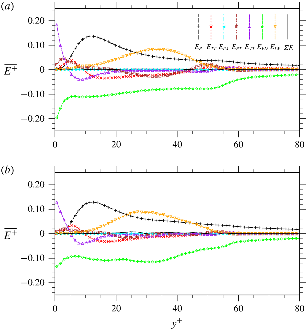
Turbulent kinetic energy budgets in single-phase and particle-laden turbulent channel flows: (a) Case 3, (b) Case 4.

Equation (4.9) is examined by the simulation results in each case. All terms in (4.9) are calculated explicitly. For conciseness, only the results from Case 3 and Case 4 are shown in figure 16. Profiles are time averaged at the statistically stationary state over 18 eddy turnover times and they are normalized by the friction velocity  $u_{\unicode[STIX]{x1D70F}}$ and wall unit in the single-phase case. The black solid line in each plot represents the summation of all terms on the right-hand side of (4.9). By theory, after being time averaged over a sufficiently long time, the summation should be identically zero as a balance is achieved. This balance has been well captured in all particle-laden cases. This supports the accuracy of the TKE budget analyses performed in the present study. While the possibility that errors generated in the computation of different terms cancel out cannot be fully excluded, this scenario is unlikely. This is because the numerical method used to conduct the simulations, which is the lattice Boltzmann method, does not have the same accuracy for the velocity, pressure and stress computations. The velocity field has a second-order accuracy while the pressure only has a first-order accuracy. The stress tensor (
 $\unicode[STIX]{x1D70F}_{ij}$ in (4.9)) in LBM can also have a second-order accuracy if it is computed directly from the non-equilibrium distribution functions (see Yong, Luo et al. Reference Yong and Luo2012), which makes the dissipation rate computation also of the second-order accuracy. However, the transport terms in (4.9) have to be computed via finite-difference approximations. Therefore, the magnitudes of errors in each term in (4.9) can hardly be of the same order to be cancelled out in the end.
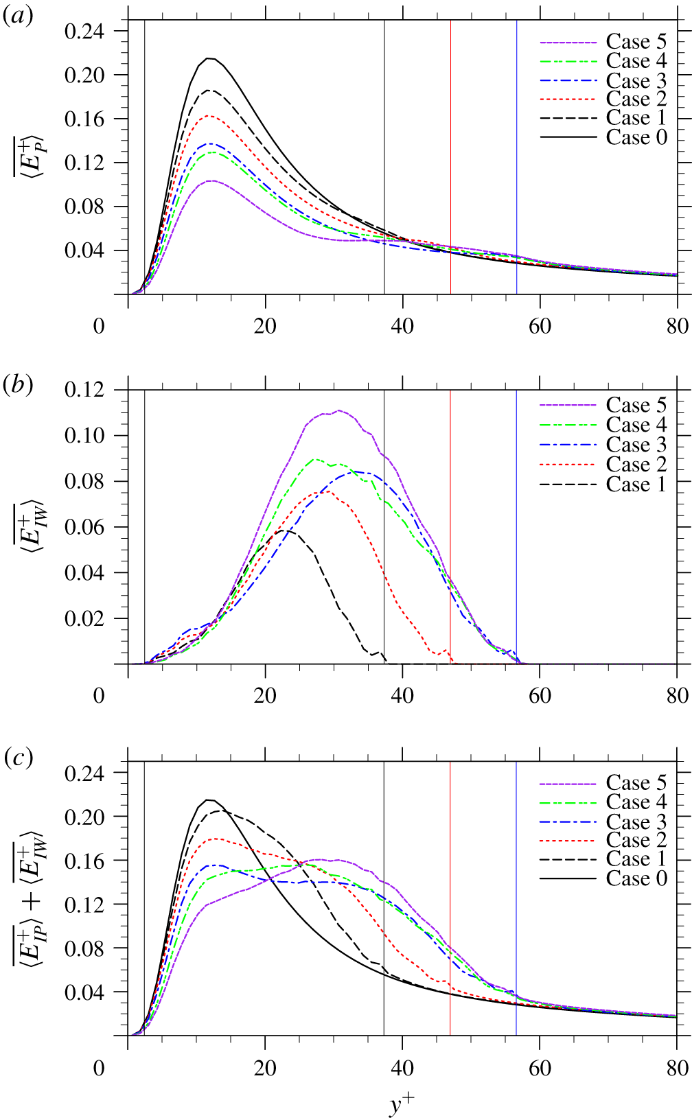
Profiles of TKE generation rate: (a) TKE production rate  $\overline{\langle E_{P}^{+}\rangle }$, (b) TKE generation due to flow displacement
 $\overline{\langle E_{IW}^{+}\rangle }$, panel (c) shows panels (a) and (b) combined.

The value of each non-trivial term in the TKE budget equations in the single-phase and particle-laden cases are then compared in detail. To consider that fluid volumes are slightly different in each case, the volume-averaged results in (4.9) are further normalized by the local fluid volume fraction, i.e. phase averaged. The profiles of  $\overline{\langle E_{P}^{+}\rangle }$ from Case 0 to Case 5 are compared in figure 17(a). By definition, the change of
 $\overline{\langle E_{P}^{+}\rangle }$ can be predicted from the modulations of Reynolds stress and viscous stress shown in figures 9 and 10, respectively. Almost in the whole region of
 $y^{+}\leqslant l_{y,max}^{+}$, the Reynolds stress and the viscous stress are reduced by the presence of the particles, so is the TKE production rate. It should be emphasized that terms in (4.9) are volume averaged rather than phase averaged, which means a certain part of the reduction simply comes from the reduced amount of fluid in the same control volume
 $V$. However, since the volume fractions are small, this contribution could be ignored. In our previous study of turbulent channel flow laden with freely moving particles (see Peng et al. Reference Peng, Ayala and Wang2019b), a similar reduction of the intrinsic TKE production
 $\overline{\langle E_{P}^{+}\rangle }$ was also observed, but was less significant. This is because freely moving particles provide much less drag to the flow, resulting in smaller reductions of both the viscous stress and Reynolds stress. In a region around
 $y^{+}=l_{y,max}^{+}$,
 $\overline{\langle E_{P}^{+}\rangle }$ is slightly enhanced. This is attributed to the slightly enhanced mean velocity gradient due to the boundary layers on the particle surfaces, as observed in figure 10.
In additional to  $E_{P}$,
 $E_{IW}$ serves as an extra source generating TKE from the mean flow. The profiles of
 $\overline{\langle E_{IW}^{+}\rangle }$ in the five particle-laden cases are shown in figure 17(b). By definition, this mechanism is only non-zero in the region where the particle hydrodynamic force on the fluid phase is non-zero. Since the hydrodynamic force exerted on the fluid phase by particles acts in the opposite direction to the flow,
 $\overline{\langle E_{IW}^{+}\rangle }$ is always positive, which transfers energy from the mean flow to sustain turbulence. The additional production of TKE via
 $E_{IW}$ was also reported by Santarelli et al. (Reference Santarelli, Roussel and Fröhlich2016) in a bubbly turbulent channel flow, and by Vreman & Kuerten (Reference Vreman and Kuerten2018) in a turbulent channel flow passing an array of particles. As mentioned earlier and also analysed in Vreman & Kuerten (Reference Vreman and Kuerten2018), the mechanism is essentially a non-turbulent effect due to flow displacements by particles. However, the difference is that, in a turbulent flow, such disturbance flows and particle wakes cannot be dissipated immediately and, as such, contribute also partially to the production of turbulent velocity fluctuations. Positive values of
 $\overline{\langle E_{IW}^{+}\rangle }$ were also reported in our previous study with freely moving particles (see Peng et al. Reference Peng, Ayala and Wang2019b), but were contributed by the particle work associated with particle translational fluctuation and particle rotation in the spanwise direction. With freely moving particles, the particle Reynolds number may not be sufficiently large to cause strong flow displacement as in the present study with fixed particles.
The combination of  $E_{P}$ and
 $E_{IW}$ represents the total production rate of TKE from the mean flow, whose time-averaged profiles are presented in figure 17(c). The shapes of the
 $\overline{\langle E_{P}^{+}+E_{IW}^{+}\rangle }$ profiles in the particle-laden cases have good similarities with the corresponding profiles of TKE, which implies that the modulation of TKE production serves as a main contributor to overall TKE modulation. However, it must be clear that terms in the TKE budget equation only represent the changing rate of TKE, which does not necessarily map to the modulation of TKE itself, but a certain degree of logical connection between the two can still be expected.
Profiles of TKE dissipation rate  $\overline{\langle E_{VD}^{+}\rangle }$.

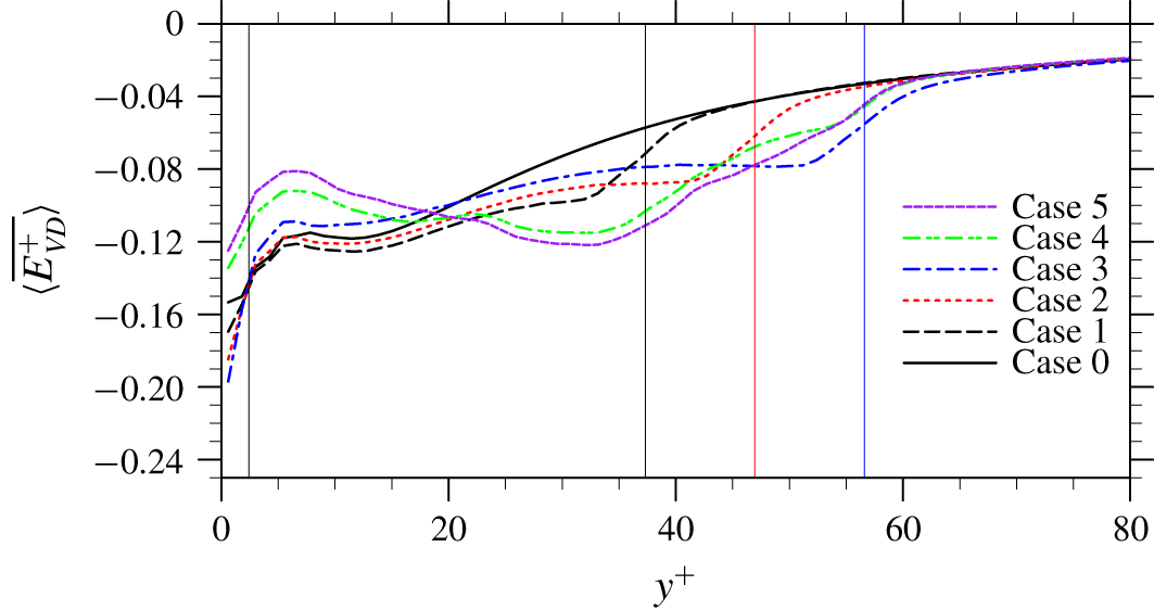
The profiles of time-averaged viscous dissipation rate  $\overline{\langle E_{VD}^{+}\rangle }$ are presented in figure 18. In Case 1 and Case 2, enhanced magnitudes of the dissipation rate are realized almost everywhere with the presence of particles. From Case 3 to Case 5, however, reduced local dissipation rates are observed in the region of
 $y^{+}\lessapprox 20$. Indeed, particles do bring an additional dissipation rate to the flow as discontinuity has been created on the two sides a fluid–particle interface, but the local dissipation rate also needs to balance with the TKE input from either local production or spatial transport. The reduction of local dissipation rate described above comes probably from the fact that the TKE generation from the mean flow has been significantly reduced at the same location, as shown in figure 17(c). The integrated dissipation rates over the whole channel in the present single-phase and particle-laden cases are given in the last column of table 3. The overall dissipation rates are enhanced in all five particle-laden cases, when compared to the single-phase counterpart.
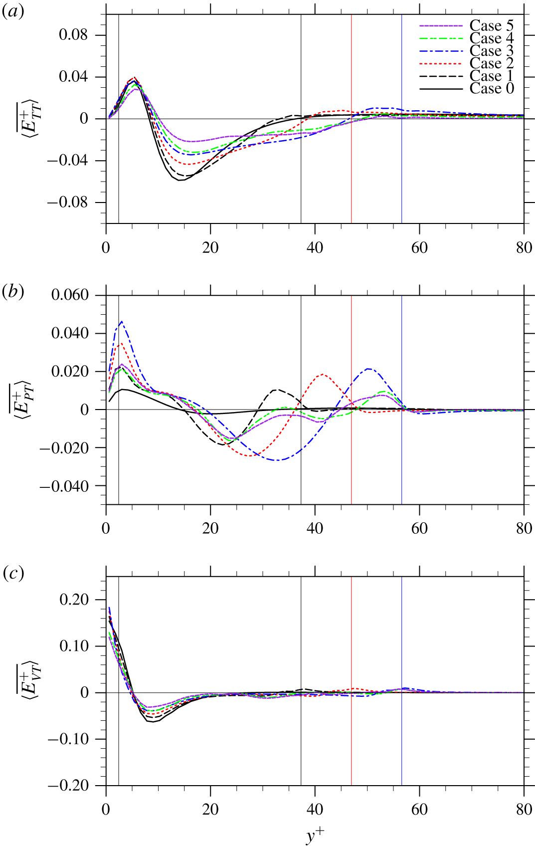
The transport of TKE along the inhomogeneous wall-normal direction is also altered by the presence of particles. In fact, even when the background flow is homogeneous, the presence of particles could alter the homogeneity of the flow and induce a certain level of TKE transport. For example, Vreman (Reference Vreman2016) discovered that an array of fixed particles in a homogeneous isotropic turbulence can trigger a strong transport of TKE from far field to the particle surfaces to supply the enhanced dissipation rate in the regions around particles. There are three transport mechanisms in both single-phase and particle-laden turbulent channel flows, turbulent transport  $E_{TT}$ due to turbulent fluctuation, pressure transport
 $E_{PT}$ due to pressure fluctuation and viscous transport
 $E_{VT}$ due to viscous diffusion, whose time-averaged profiles are presented in figures 19(a), 19(b) and 19(c), respectively.
Profiles of TKE transport rate (a) turbulent transport  $\overline{\langle E_{TT}^{+}\rangle }$, (b) pressure transport
 $\overline{\langle E_{PT}^{+}\rangle }$, (c) viscous transport
 $\overline{\langle E_{VT}^{+}\rangle }$.

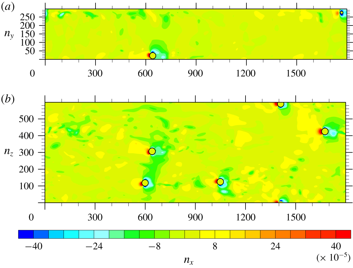
Snapshots of the pressure contour from Case 3 on: (a) a wall-normal cut at a spanwise location  $z=L_{z}/2$, and (b) a spanwise cut at a wall-normal location
 $y=l_{y,min}+0.5d_{p}$.

The turbulent transport mechanism  $E_{TT}$ in a single-phase turbulent channel flow conveys TKE from the buffer region to the viscous sublayer. In particle-laden cases,
 $\overline{\langle E_{TT}^{+}\rangle }$ is altered mainly in the region between
 $y^{+}\approx 10$ and
 $y^{+}\approx l_{y,max}^{+}$, where the turbulence intensity is modified most significantly. The changes of
 $\overline{\langle E_{TT}^{+}\rangle }$ in each particle-laden case are in good correlation with the corresponding changes of TKE shown in figure 12. Less TKE is transported out from the region
 $10\lessapprox y^{+}\lessapprox 25$, where TKE is significantly reduced. On the contrary, more TKE is transported out from the region
 $25\lessapprox y^{+}\leqslant l_{y,max}^{+}$, in which TKE is enhanced.
The pressure transport mechanism  $E_{PT}$ is generally weak in a single-phase turbulent channel flow. However, when particles are present, the intensity of this transport is greatly strengthened in the whole region of
 $y^{+}\leqslant l_{y,max}^{+}$. This is because when the flow ceases at the front edges of the static particles, a high local pressure forms, which drives more TKE from the plane of the stagnation point to the surrounding area. A similar observation that particles greatly enhance the pressure transport of TKE was also reported by Vreman & Kuerten (Reference Vreman and Kuerten2018). To confirm, a wall-normal (
 $x{-}y$) cut at a spanwise location
 $z=L_{z}/2$ and a spanwise (
 $x{-}z$) cut at a wall-normal location
 $y=l_{y,min}+0.5d_{p}$ of the pressure field in Case 3 are shown in figure 20. There are clearly high pressure fluctuations on the leading edge of each fixed particle and low pressure fluctuations in the surrounding areas. In the first three cases, particles are placed around the same wall-normal location in each case, the profile of
 $\overline{\langle E_{PT}^{+}\rangle }$ in each case exhibits a trough with the strongest outward transport at the wall-normal location roughly corresponding to the particle centre plane. At the same time, two crests with strongest inward transport form on the two sides of the particle centre plane. In the last two cases, since the particles are distributed in a wider range of wall-normal locations, the profiles of
 $\overline{\langle E_{PT}^{+}\rangle }$ exhibit multiple troughs and crests. It is also worth mentioning that in our previous study with freely moving particles, an enhanced pressure transport
 $\overline{\langle E_{PT}^{+}\rangle }$ was also identified. However, in that case, the enhancement was mainly contributed by the particle rotation in the spanwise direction (see Peng et al. Reference Peng, Ayala and Wang2019b). The particle Reynolds number of the freely moving particles was found to be less than 30 in most regions of the channel. This particle Reynolds number may be too small to introduce the strong flow disturbance that is found in this study.
Finally, the viscous transport  $E_{VT}$ is only important near the channel walls where the viscous effect is important. In both the single-phase and the particle-laden cases, this region roughly corresponds to
 $y^{+}\leqslant 20$. In the single-phase turbulent channel flow,
 $E_{VT}$ acts as one of the main mechanisms that transports TKE from the buffer region, where the majority of TKE is generated, to the near-wall region, where the strongest viscous dissipation takes place. In general, the intensity of
 $E_{VT}$ in
 $y^{+}\leqslant 20$ has been reduced by the particles, as shown in figure 19(c). Less TKE is transported out from the buffer region to the near-wall region. This is because the presence of the particles leads to a more homogeneous distribution of TKE locally (see figure 12), which weakens the viscous diffusion of TKE. A slightly enhanced
 $\overline{\langle E_{VT}^{+}\rangle }$ can be identified around
 $y^{+}=l_{y,max}^{+}$ in each case. This enhancement is likely due to the boundary layers developed on the particle surface, which is consistent with the observation by Vreman & Kuerten (Reference Vreman and Kuerten2018).
Combining the three transport mechanisms together, the profiles of total TKE transport in the wall-normal direction are given in figure 21. The net TKE transport rate over the whole channel, defined as  $1/H\int _{0}^{H}(|\overline{\langle E_{TT}^{+}\rangle }+\overline{\langle E_{PT}^{+}\rangle }+\overline{\langle E_{VT}^{+}\rangle }|)\,\text{d}y$, is found to be
 $0.0132$,
 $0.0144$,
 $0.0153$,
 $0.0162$,
 $0.0118$,
 $0.0109$ from Case 0 to Case 5. In the first three particle-laden cases, particles enhance the transport of TKE in the wall-normal direction. In the last two particle-laden cases, the opposite happens.
Profiles of total transport rate of TKE in particle-laden turbulent flow simulations.

Due to the anisotropic distribution of TKE among different velocity components in a turbulent channel flow, inter-component exchanges of TKE also take place. In a single-phase turbulent channel flow, the wall-normal and spanwise velocity fluctuations do not come directly from the mean flow, but are originated from the streamwise velocity fluctuation through the coupling between the pressure fluctuation and strain rate fluctuation. When particles are present, this inter-component transfer mechanism of TKE is also modified. The component-wise TKE budget equations in a particle-laden turbulent channel flow read as follows.
Streamwise:
 $$\begin{eqnarray}\displaystyle & & \displaystyle \frac{\unicode[STIX]{x2202}}{\unicode[STIX]{x2202}t}\unicode[STIX]{x1D6FC}\frac{1}{2}\langle u_{x}^{\prime }u_{x}^{\prime }\rangle =\underbrace{-\unicode[STIX]{x1D6FC}\langle u_{x}^{\prime }u_{y}^{\prime }\rangle \frac{\unicode[STIX]{x2202}\langle u_{x}\rangle }{\unicode[STIX]{x2202}y}}_{E_{Px}}\underbrace{-\frac{\unicode[STIX]{x2202}}{\unicode[STIX]{x2202}y}\left[\unicode[STIX]{x1D6FC}\frac{1}{2}\langle u_{x}^{\prime }u_{x}^{\prime }u_{y}^{\prime }\rangle \right]}_{E_{TTx}}\underbrace{+\frac{1}{\unicode[STIX]{x1D70C}}\frac{\unicode[STIX]{x2202}}{\unicode[STIX]{x2202}y}\left[\unicode[STIX]{x1D6FC}\langle \unicode[STIX]{x1D70F}_{xy}^{\prime }u_{x}^{\prime }\rangle \right]}_{E_{VTx}}\nonumber\\ \displaystyle & & \displaystyle \quad +\,\underbrace{\frac{\unicode[STIX]{x1D6FC}}{\unicode[STIX]{x1D70C}}\left\langle p^{\prime }\frac{\unicode[STIX]{x2202}u_{x}^{\prime }}{\unicode[STIX]{x2202}x}\right\rangle }_{E_{PSx}}\underbrace{-\frac{\unicode[STIX]{x1D6FC}}{\unicode[STIX]{x1D70C}}\left(\left\langle \unicode[STIX]{x1D70F}_{xx}^{\prime }\frac{\unicode[STIX]{x2202}u_{x}^{\prime }}{\unicode[STIX]{x2202}x}\right\rangle +\left\langle \unicode[STIX]{x1D70F}_{xy}^{\prime }\frac{\unicode[STIX]{x2202}u_{x}^{\prime }}{\unicode[STIX]{x2202}y}\right\rangle +\left\langle \unicode[STIX]{x1D70F}_{xz}^{\prime }\frac{\unicode[STIX]{x2202}u_{x}^{\prime }}{\unicode[STIX]{x2202}z}\right\rangle \right)}_{E_{VDx}}\nonumber\\ \displaystyle & & \displaystyle \quad +\,\underbrace{\left[\frac{\unicode[STIX]{x1D6FC}}{\unicode[STIX]{x1D70C}}\langle p\rangle \left\langle \frac{\unicode[STIX]{x2202}u_{x}}{\unicode[STIX]{x2202}x}\right\rangle +\frac{\unicode[STIX]{x1D6FC}}{\unicode[STIX]{x1D70C}}\langle \unicode[STIX]{x1D70F}_{xy}\rangle \frac{\unicode[STIX]{x2202}\langle u_{x}\rangle }{\unicode[STIX]{x2202}y}-\frac{\unicode[STIX]{x1D6FC}}{\unicode[STIX]{x1D70C}}\left(\!\langle \unicode[STIX]{x1D70F}_{xx}\rangle \left\langle \frac{\unicode[STIX]{x2202}u_{x}}{\unicode[STIX]{x2202}x}\right\rangle +\langle \unicode[STIX]{x1D70F}_{xy}\rangle \left\langle \frac{\unicode[STIX]{x2202}u_{x}}{\unicode[STIX]{x2202}y}\right\rangle +\langle \unicode[STIX]{x1D70F}_{xz}\rangle \left\langle \frac{\unicode[STIX]{x2202}u_{x}}{\unicode[STIX]{x2202}z}\right\rangle \!\right)\!\right]}_{E_{IMx}}\nonumber\\ \displaystyle & & \displaystyle \quad +\,\underbrace{\frac{1}{\unicode[STIX]{x1D70C}V}\int _{S_{I}}n_{j}(-p\unicode[STIX]{x1D6FF}_{xj}u_{x}+u_{x}\unicode[STIX]{x1D70F}_{xj})\,\text{d}S-\frac{1}{\unicode[STIX]{x1D70C}V}\langle u_{x}\rangle \int _{S_{I}}n_{j}(-p\unicode[STIX]{x1D6FF}_{xj}+\unicode[STIX]{x1D70F}_{xj})\,\text{d}S}_{E_{IWx}},\end{eqnarray}$$
transverse:
 $$\begin{eqnarray}\displaystyle & & \displaystyle \frac{\unicode[STIX]{x2202}}{\unicode[STIX]{x2202}t}\unicode[STIX]{x1D6FC}\frac{1}{2}\langle u_{y}^{\prime }u_{y}^{\prime }\rangle =\underbrace{-\frac{\unicode[STIX]{x2202}}{\unicode[STIX]{x2202}y}\left[\unicode[STIX]{x1D6FC}\frac{1}{2}\langle u_{y}^{\prime }u_{y}^{\prime }u_{y}^{\prime }\rangle \right]}_{E_{TTy}}\underbrace{-\frac{1}{\unicode[STIX]{x1D70C}}\frac{\unicode[STIX]{x2202}}{\unicode[STIX]{x2202}y}[\unicode[STIX]{x1D6FC}\langle p^{\prime }u_{y}^{\prime }\rangle ]}_{E_{PTy}}\underbrace{+\frac{1}{\unicode[STIX]{x1D70C}}\frac{\unicode[STIX]{x2202}}{\unicode[STIX]{x2202}y}[\unicode[STIX]{x1D6FC}\langle \unicode[STIX]{x1D70F}_{yy}^{\prime }u_{y}^{\prime }\rangle ]}_{E_{VTy}}\nonumber\\ \displaystyle & & \displaystyle \quad +\,\underbrace{\frac{\unicode[STIX]{x1D6FC}}{\unicode[STIX]{x1D70C}}\left\langle p^{\prime }\frac{\unicode[STIX]{x2202}u_{y}^{\prime }}{\unicode[STIX]{x2202}y}\right\rangle }_{E_{PSy}}\underbrace{-\frac{\unicode[STIX]{x1D6FC}}{\unicode[STIX]{x1D70C}}\left(\left\langle \unicode[STIX]{x1D70F}_{xy}^{\prime }\frac{\unicode[STIX]{x2202}u_{y}^{\prime }}{\unicode[STIX]{x2202}x}\right\rangle +\left\langle \unicode[STIX]{x1D70F}_{yy}^{\prime }\frac{\unicode[STIX]{x2202}u_{y}^{\prime }}{\unicode[STIX]{x2202}y}\right\rangle +\left\langle \unicode[STIX]{x1D70F}_{yz}^{\prime }\frac{\unicode[STIX]{x2202}u_{y}^{\prime }}{\unicode[STIX]{x2202}z}\right\rangle \right)}_{E_{VDy}}\nonumber\\ \displaystyle & & \displaystyle \quad +\,\underbrace{\left[\frac{\unicode[STIX]{x1D6FC}}{\unicode[STIX]{x1D70C}}\langle p\rangle \left\langle \frac{\unicode[STIX]{x2202}u_{y}}{\unicode[STIX]{x2202}y}\right\rangle -\frac{\unicode[STIX]{x1D6FC}}{\unicode[STIX]{x1D70C}}\left(\langle \unicode[STIX]{x1D70F}_{xy}\rangle \left\langle \frac{\unicode[STIX]{x2202}u_{y}}{\unicode[STIX]{x2202}x}\right\rangle +\langle \unicode[STIX]{x1D70F}_{yy}\rangle \left\langle \frac{\unicode[STIX]{x2202}u_{y}}{\unicode[STIX]{x2202}y}\right\rangle +\langle \unicode[STIX]{x1D70F}_{yz}\rangle \left\langle \frac{\unicode[STIX]{x2202}u_{y}}{\unicode[STIX]{x2202}z}\right\rangle \right)\right]}_{E_{IMy}}\nonumber\\ \displaystyle & & \displaystyle \quad +\,\underbrace{\frac{1}{\unicode[STIX]{x1D70C}V}\int _{S_{I}}n_{j}(-p\unicode[STIX]{x1D6FF}_{yj}u_{y}+u_{y}\unicode[STIX]{x1D70F}_{yj})\,\text{d}S}_{E_{IWy}},\end{eqnarray}$$
spanwise:
 $$\begin{eqnarray}\displaystyle & & \displaystyle \frac{\unicode[STIX]{x2202}}{\unicode[STIX]{x2202}t}\unicode[STIX]{x1D6FC}\frac{1}{2}\langle u_{z}^{\prime }u_{z}^{\prime }\rangle =\underbrace{-\frac{\unicode[STIX]{x2202}}{\unicode[STIX]{x2202}y}\left[\unicode[STIX]{x1D6FC}\frac{1}{2}\langle u_{z}^{\prime }u_{z}^{\prime }u_{y}^{\prime }\rangle \right]}_{E_{TTz}}\underbrace{+\frac{1}{\unicode[STIX]{x1D70C}}\frac{\unicode[STIX]{x2202}}{\unicode[STIX]{x2202}y}[\unicode[STIX]{x1D6FC}\langle \unicode[STIX]{x1D70F}_{yz}^{\prime }u_{z}^{\prime }\rangle ]}_{E_{VTz}}\nonumber\\ \displaystyle & & \displaystyle \quad +\,\underbrace{\frac{\unicode[STIX]{x1D6FC}}{\unicode[STIX]{x1D70C}}\left\langle p^{\prime }\frac{\unicode[STIX]{x2202}u_{z}^{\prime }}{\unicode[STIX]{x2202}z}\right\rangle }_{E_{PSz}}\underbrace{-\frac{\unicode[STIX]{x1D6FC}}{\unicode[STIX]{x1D70C}}\left(\left\langle \unicode[STIX]{x1D70F}_{xz}^{\prime }\frac{\unicode[STIX]{x2202}u_{z}^{\prime }}{\unicode[STIX]{x2202}x}\right\rangle +\left\langle \unicode[STIX]{x1D70F}_{yz}^{\prime }\frac{\unicode[STIX]{x2202}u_{z}^{\prime }}{\unicode[STIX]{x2202}y}\right\rangle +\left\langle \unicode[STIX]{x1D70F}_{zz}^{\prime }\frac{\unicode[STIX]{x2202}u_{z}^{\prime }}{\unicode[STIX]{x2202}z}\right\rangle \right)}_{E_{VDz}}\nonumber\\ \displaystyle & & \displaystyle \quad +\,\underbrace{\left[\frac{\unicode[STIX]{x1D6FC}}{\unicode[STIX]{x1D70C}}\langle p\rangle \left\langle \frac{\unicode[STIX]{x2202}u_{z}}{\unicode[STIX]{x2202}z}\right\rangle -\frac{\unicode[STIX]{x1D6FC}}{\unicode[STIX]{x1D70C}}\left(\langle \unicode[STIX]{x1D70F}_{xz}\rangle \left\langle \frac{\unicode[STIX]{x2202}u_{z}}{\unicode[STIX]{x2202}x}\right\rangle +\langle \unicode[STIX]{x1D70F}_{yz}\rangle \left\langle \frac{\unicode[STIX]{x2202}u_{z}}{\unicode[STIX]{x2202}y}\right\rangle +\langle \unicode[STIX]{x1D70F}_{zz}\rangle \left\langle \frac{\unicode[STIX]{x2202}u_{z}}{\unicode[STIX]{x2202}z}\right\rangle \right)\right]}_{E_{IMz}}\nonumber\\ \displaystyle & & \displaystyle \quad +\,\underbrace{\frac{1}{\unicode[STIX]{x1D70C}V}\int _{S_{I}}n_{j}(-p\unicode[STIX]{x1D6FF}_{zj}u_{z}+u_{z}\unicode[STIX]{x1D70F}_{zj})\,\text{d}S}_{E_{IWz}},\end{eqnarray}$$
where the subscripts  $x$,
 $y$,
 $z$ are used to distinguish terms in each equation. Since the particles are fixed, the terms related to the particle movement,
 $E_{IMi}$,
 $E_{IWy}$ and
 $E_{IWz}$, are still expected to be zero. The same as the single-phase case, in the particle-laden cases, there is still no direct TKE input from the mean flow to the wall-normal and spanwise velocity fluctuations. The TKE generated from the mean flow through production and particle displacement is originally streamwise TKE, and is then transferred to the other two directions. The changes of turbulent intensity in the wall-normal and spanwise velocity components still must be manifested through the modifications of the corresponding pressure–strain rate term.
Component-wise turbulent kinetic energy budgets in Case 4: (a) streamwise, (b) transverse, (c) spanwise.

The simulated component-wise TKEs and dissipation rates.

The streamwise, wall-normal and spanwise TKE budget equations are examined with the DNS data in each case. For conciseness, only the overall balances of component-wise TKE in Case 4 are presented in figure 22. The black solid line in each figure represents the summation of all the terms on the right-hand sides of (4.10a)–(4.10c). Again, the black lines in figure 22 are essentially zero with only minor errors. We thus conclude that the results of the component-wise TKE budgets presented here are reasonably accurate. In our previous study with freely moving particles, particle rotation was found to directly transfer TKE to the wall-normal component (see Peng et al. Reference Peng, Ayala and Wang2019b). However, in the current simulations with fixed particles, there is no such mechanism. TKE is still first obtained by the streamwise velocity component then transferred to the other two components through the pressure–strain rate coupling.
The component-wise TKE and dissipation rates integrated over the whole channel in each case are summarized in table 4. In terms of the absolute value, the modulations of component-wise TKE are not significant, except the streamwise TKE in Case 4 and Case 5, where attenuation of approximately 10 % is observed. The percentage of component-wise TKE occupying the total TKE is shown in parentheses in table 4. The modulation in terms of the percentage is approximately 1 %–2 %. The component-wise dissipation rates, however, are generally enhanced for all three directions in the particle-laden cases. Since TKE cannot be transferred directly from the mean flow to the wall-normal and spanwise directions, there must be an augmented inter-component transfer of TKE from the streamwise component to accommodate the enhanced dissipation rates in the wall-normal and spanwise directions. In terms of percentages, it is interesting to observe that the dissipation rate is slightly more anisotropic than the TKE, reflecting the fact that the anisotropy is generated in the near-wall region through the small-scale shear flow instability.
Profiles of the pressure–strain rate terms for different velocity components: (a) streamwise, (b) wall-normal, (c) spanwise. The zigzag profile of  $\overline{\langle E_{PSz}\rangle }^{+}$ in the single-phase case is probably due to the acoustic waves associated with the weak compressibility in the LBM.

The profiles of the time-averaged pressure–strain rate term in each component-wise TKE budget equation are summarized in figure 23. Compared to the single-phase turbulent channel flow, in all particle-laden flows, the overall intensity of the inter-component TKE transfers among different velocity components are greatly strengthened, as expected. The modulations brought by the particles vary with the wall-normal location and can be roughly divided into three distinct sections.
The first section covers the region from  $y^{+}\approx 15$ to
 $y^{+}\approx l_{y,max}^{+}-10$, which roughly corresponds to the wall-normal locations of the buffer region in the single-phase case. In this section, the presence of particles significantly enhances the inter-component TKE transfer from the streamwise velocity fluctuation to the other two velocity components. This augmentation is mainly because particles inhibit the streamwise motions by blocking the incoming flows and creating wall-normal and spanwise motions around their surfaces. The wakes generated after the particles could also contain more wall-normal and spanwise motions than the undisturbed flow in a single-phase turbulent channel flow. As a result, the maximum intensity of the inter-component transfer should occur around the wall-normal location corresponding to the planes cutting through the centres of solid particles, i.e.
 $y^{+}\approx (l_{y,max}^{+}+l_{y,min}^{+})/2$ in each case. This is confirmed in figure 23(a) with the simulation results.
The second section spans from the channel wall to  $y^{+}\approx 15$. In this section, the wall-normal velocity component loses significantly more TKE, and part of this TKE is received by the streamwise velocity component. This transfer of TKE from the wall-normal direction to the streamwise direction does not occur in the single-phase case. This new mechanism happens because the wall-normal velocity component in the first section received much more TKE from the streamwise direction, and this TKE is transported towards the channel wall through a significantly enhanced pressure transport. When this wall-normal TKE arrives the channel wall, it is not dissipated but transferred to the other two directions due to the spherical shape of particles and the non-penetrable channel walls. The inter-component transfer of TKE received by the spanwise velocity component in this section is also generally enhanced by the presence of particles, as shown in figure 23(c).
The region from  $y^{+}\approx l_{y,max}^{+}-10$ to
 $y^{+}\approx l_{y,max}^{+}$ is the third section, where less TKE is transferred from the streamwise velocity component to the wall-normal component, compared to the single-phase turbulent channel flow. This modification is due to the same mechanism that invokes the inter-component transfer of TKE from the wall-normal component to the streamwise component in the second section, which is that more wall-normal TKE is transported from the first section to this section through an enhanced pressure transport, then transferred back to streamwise direction due to the spherical shape of the particles. In the third section, the pressure–strain rate coupling in the spanwise direction is modified only marginally.
Sketch to illustrate the role of particle regulation in the inter-component turbulent kinetic energy transfers.

To conclude the above analyses, a sketch of how particles alter the local flow and thus affect the inter-component TKE transfer of wall-generated turbulence is provided in figure 24. Fixed particles force the incoming flow to move sideways, and thus enhance the inter-component TKE transfer from the streamwise velocity component to the other two components. Part of this kinetic energy may eventually be returned to the streamwise component, due to the spherical shape of the particles, and the constraint imposed by the channel wall on the wall-normal fluid motions.
5 Summary and conclusions
In this paper, IR-DNS based on LBM were used to study the flow modulations due to a few fixed particles in a turbulent channel flow. This relatively simple configuration provides a powerful setting to accurately probe and quantify different mechanisms through which the finite-size solid particles modulate the fluid turbulence statistics. Particle size, total particle surface area and particle volume fraction are varied to study how the modulation effects depend on these parameters. The driving force per unit fluid volume is kept the same in all of the simulations conducted. The particles in each case are placed in a small wall-normal range so direct and intensive interactions between disturbance flows by the particles and wall-generated turbulence take place. Although the particle volume fractions are kept very small ( $\unicode[STIX]{x1D719}_{p}\ll 1\,\%$), under the present flow configuration, particles are found to significantly modulate both the mean flow and turbulence intensity. The main conclusions are summarized below.
(i) When particle volume fractions are small, the modulation of the mean flow velocity scales approximately with the total particle surface area. With a fixed driving force, particles significantly reduce not only the average flow speed but also the friction velocity at the channels walls.
(ii) The modulation of the mean velocity profiles can be analysed with a stress balance analysis. In the region around the channel centre, where particles are not present, the stress balance in the particle-laden cases is identical to that in the single-phase flow. Under this condition, the viscous stress is almost unaltered in the particle-laden cases and an unaltered slope of velocity profiles in the log-law region is therefore produced. In the viscous sublayer, on the other hand, the mean flow velocity still scales linearly with the distance from the wall, but with a reduced slope.
(iii) The modulations brought by solid particles to the turbulent kinetic energy are also significant. The addition of particles generally results in a more homogeneous TKE distribution in the wall-normal direction, and a more isotropic TKE distribution among the three velocity components in the particle-laden cases. These observations are similar to the recent results for turbulent channel flows with freely moving particles (see Picano et al. Reference Picano, Breugem and Brandt2015; Eshghinejadfard et al. Reference Eshghinejadfard, Abdelsamie, Hosseini and Thévenin2017; Peng et al. Reference Peng, Ayala and Wang2019b), but different from the studies of Kulick et al. (Reference Kulick, Fessler and Eaton1994) and Vreman & Kuerten (Reference Vreman and Kuerten2018), where the anisotropy was found to be increased by the particles.
(iv) The modulations of the turbulence intensity can be understood through a complete TKE budget analysis applied to the particle-laden flows. The presence of particles plays dual roles in the transfer of kinetic energy from the mean flow to TKE, i.e. significantly decreasing the intrinsic TKE production by reducing both the mean shear rate and the Reynolds stress, but at the same time creating a TKE generation mechanism via disturbance flows and particle wakes. The later mechanism is found to be much stronger than that in our earlier study with freely moving particles (Peng et al. Reference Peng, Ayala and Wang2019b), where the weaker disturbances are mainly associated with the fluctuations in particle translation and particle rotation. The local dissipation rate is modified to accommodate the changes of local TKE input and TKE transport, which is not necessarily always enhanced by the presence of particles.
(v) Particles also alter the transport of TKE in the inhomogeneous (i.e. wall-normal) direction. The level of modulation of the turbulent transport term follows the change in the level of the local turbulence fluctuations. The pressure transport is significantly strengthened by particles due to the formation of high and low pressure regions around the stagnation points where the fluid velocity ceases on the fixed particle surfaces, similar to observations made by Vreman & Kuerten (Reference Vreman and Kuerten2018). This is in contrast to our earlier study with freely moving particles (Peng et al. Reference Peng, Ayala and Wang2019b), where particle rotation was found to be the main reason for the enhancement of pressure transport. The viscous transport is generally attenuated, as the presence of particles homogenizes the wall-normal distribution of TKE.
(vi) Finally, the component-wise TKE budget analysis reveals that the inter-component transfer of TKE was also significantly modified by the presence of particles. With fixed particles, TKE is still first obtained by the streamwise velocity component, then transferred to the other two components, the same as in the unladen case. This differs from the observation in our earlier study with freely moving particles, where the wall-normal velocity component can directly receive TKE from the mean flow due to particle rotation (Peng et al. Reference Peng, Ayala and Wang2019b). In the present case with fixed particles, more TKE is transferred from the streamwise velocity to the other two components around the locations corresponding to the particle centres. Aside from that plane, the inverse transfer of TKE from the wall-normal direction to the streamwise direction takes place. The latter mechanism does not exist in single-phase turbulent channel flows.
We also note that additional simulations with the same fixed particle centre locations but with free particle rotations were performed; it was found that particle rotation has a negligible effect on the resulting mean flow and turbulence statistics, due to the very small particle volume fractions studied in this work.
In conclusion, this study demonstrates that much insight into the flow modulation by solid particles can be derived from interface-resolved DNS. The techniques of stress and TKE budget analyses could serve as useful tools to understand flow modulation by solid particles at a more in-depth level. Both the total and component-wise TKE and dissipation rates are documented fully, in the hope that these data can be used to guide future modelling studies of flow modulation by solid particles. Fixed particles in a turbulent flow usually imply much larger particle Reynolds numbers than freely moving particles, as such fixed particles can result in significant flow displacements and wake effects. Comparing the flow modulation mechanisms observed with fixed particles in this work and those observed with freely moving particles in Peng et al. (Reference Peng, Ayala and Wang2019b) helps us better understand the roles of different aspects of particle motion and particle Reynolds number in turbulence modulation.
Acknowledgements
The authors would like to acknowledge the valuable comments and suggestions provided by Dr B. de Motta from the CORIA Laboratory at the Normandy University in France. This work has been supported by the National Natural Science Foundation of China (91852205, 91741101 and 11961131006), and by the US National Science Foundation (NSF) under grants CNS1513031 and CBET-1706130. Acknowledgment is made by O.M.A. to the donors of the American Chemical Society Petroleum Research Fund for partial support of this research. Computing resources are provided by Center for Computational Science and Engineering of Southern University of Science and Technology and by National Center for Atmospheric Research through CISL-P35751014, and CISL-UDEL0001.
Declaration of interests
The authors report no conflict of interest.
Appendix A. The physical locations of particles
In this appendix, for completeness we provide the locations of particles in all five cases. This information is needed if others wish to reproduce the results presented in this document.
Particle locations in Case 1–Case 3. Particles in these three cases have identical streamwise and spanwise locations, but different wall-normal locations. The three numbers under the  $y/L_{y}$ are the particle wall-normal locations in Case 1, Case 2 and Case 3, respectively.

Particle locations in Case 4.

Particle locations in Case 5.

Appendix B. Information on the D3Q27 MRT LBM model
The definitions of equilibrium moments, forcing terms and the values of relaxation parameters in the D3Q27 MRT model. Here  $\boldsymbol{u}=(u,v,w)$ and
 $\boldsymbol{F}=(F_{x},F_{y},F_{z})$ are the local hydrodynamic velocity and body force, respectively.

The definitions of equilibrium moments, forcing terms and the values of the relaxation parameters in the D3Q27 MRT model are provided in table 8. It should be emphasized that LBM solves a larger system compared to the Navier–Stoke equations. Therefore, although definitions of all the equilibrium moments and forcing terms and values of all of the relaxation parameters are explicitly given, some of these are irrelevant to the Navier–Stokes equations, and can be defined arbitrarily in theory. These irrelevant factors are the 17–26 equilibrium moments, the 10–26 forcing terms and the 10–26 relaxation parameters. In practice, these irrelevant factors are usually adjusted to maximize the numerical stability. Adjusting these factors would not affect the physical results governed by the Navier–Stokes equations.