1 Introduction
The study of turbulent separation bubbles induced by surface-mounted bluff bodies is of both practical and theoretical importance. These separation bubbles are inherently unsteady, and exhibit regions of flow acceleration and deceleration, strong streamline curvature and elevated turbulence levels. The interplay among these features give rise to fluid motions of considerable dynamic complexity, and provides an attractive opportunity for investigating some fundamental properties of complex turbulent shear flows of engineering importance. The unsteady nature of the separation bubbles causes large pressure fluctuations (Lee & Sung Reference Lee and Sung2001; Camussi et al. Reference Camussi, Felli, Pereira, Aloisio and Di Marco2008; Graziani et al. Reference Graziani, Lippert, Uystepruyst and Keirsbulck2017). This can lead to detrimental effects in diverse engineering and environmental applications, including flapping motion and unsteady aerodynamic loads on buildings, flow-induced vibration and fatigue failure or inefficiencies in fluid-thermal devices (Wang, Zhou & Mi Reference Wang, Zhou and Mi2012; Akon & Kopp Reference Akon and Kopp2016). Turbulent flow separation has also been exploited in some applications to enhance heat transfer, improve flow-mixing properties and stabilize combustion processes (Meinders, Hanjalic & Martinuzzi Reference Meinders, Hanjalic and Martinuzzi1999; Abu-Mulaweh Reference Abu-Mulaweh2009). Motivated by these practical and fundamental considerations, flows around prototypical two-dimensional (2-D) geometries including a forward-facing step (FFS), forward–backward-facing step (FBFS) and bump (Wilhelm, Härtel & Kleiser Reference Wilhelm, Härtel and Kleiser2003; Pearson, Goulart & Ganapathisubramani Reference Pearson, Goulart and Ganapathisubramani2013; Fadla et al. Reference Fadla, Alizard, Keirsbulck, Robinet, Laval, Foucaut, Chovet and Lippert2019; Fang & Tachie Reference Fang and Tachie2019), as well as three-dimensional (3-D) surface-mounted bluff bodies such as a cube (Castro & Robins Reference Castro and Robins1977; Hussein & Martinuzzi Reference Hussein and Martinuzzi1996; Hearst, Gomit & Ganapathisubramani Reference Hearst, Gomit and Ganapathisubramani2016) have been the subject of intense research over the past decades. Nonetheless, the present understanding of the spatio-temporal dynamics of flow separations induced by surface-mounted bluff bodies with spanwise dimensions encompassing 3-D and 2-D configurations is deficient. This study presents time-resolved particle image velocimetry (TR-PIV) measurements over 2-D and 3-D surface-mounted bluff bodies with finite streamwise extent and submerged in a thick turbulent boundary layer. Of particular interest is the interaction between the separation bubbles formed on top of and behind the bluff bodies, and how this interaction and statistical properties of the shear layers change as the spanwise extent is increased progressively from a 3-D to 2-D configuration.
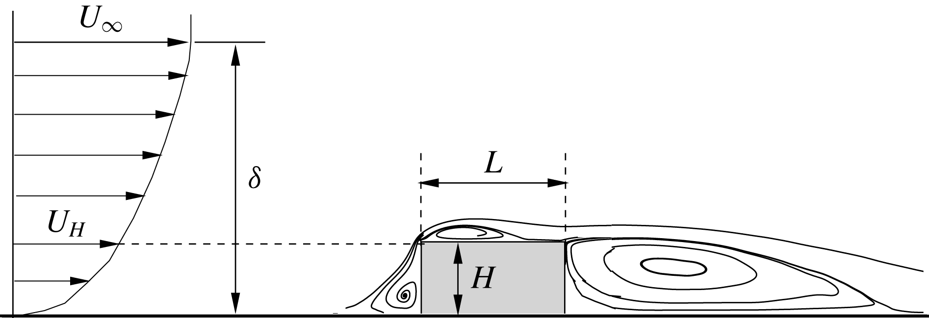
Schematic of mean streamlines over a surface-mounted bluff body (not to scale) submerged in a turbulent boundary layer with the free-stream velocity,
 $U_{\infty }$
, and thickness,
 $\unicode[STIX]{x1D6FF}$
. The streamwise and vertical dimensions of the bluff body are denoted by
 $L$
and
 $H$
, respectively, and the upstream streamwise mean velocity at the body height is denoted by
 $U_{H}$
.

Figure 1 shows a 2-D representation of a sharp-edged surface-mounted bluff body of height,
 $H$
, and length,
 $L$
, immersed in an oncoming turbulent boundary layer (TBL). The spanwise width of the body (not shown) is hereafter denoted by
 $S$
;
 $U_{\infty }$
,
 $U_{H}$
and
 $\unicode[STIX]{x1D6FF}$
, respectively, denote the free-stream velocity, streamwise mean velocity at the body height and the boundary layer thickness. The generic configuration shown in figure 1 features three distinct recirculation regions. The upstream separation bubble formed at the foot of the bluff body is a universal feature of all surface-mounted bluff bodies, including 2-D and 3-D configurations. On the contrary, a concurrent existence of distinct separation bubbles on top of and behind the body, and the dynamics of these bubbles are sensitive to the specific condition of the oncoming TBL and geometry of the bluff body (Bergeles & Athanassiadis Reference Bergeles and Athanassiadis1983; van der Kindere & Ganapathisubramani Reference van der Kindere and Ganapathisubramani2018; Chalmers et al.
Reference Chalmers, Nyantekyi-Kwakye, Fang and Tachie2019). Traditionally, the relative boundary layer thickness (
 $\unicode[STIX]{x1D6FF}/H$
) as well as turbulence intensity (
 $I_{u}=u_{rms}^{\prime }|_{y=H}$
) and mean shear (
 $T_{H}=\unicode[STIX]{x2202}U/\unicode[STIX]{x2202}y|_{y=H}$
), both evaluated at the body height, are used to characterize the oncoming TBL (Castro & Robins Reference Castro and Robins1977; Essel et al.
Reference Essel, Nematollahi, Thacher and Tachie2015; Hearst et al.
Reference Hearst, Gomit and Ganapathisubramani2016). Fully submerged surface-mounted bodies (
 $\unicode[STIX]{x1D6FF}/H>1$
) are subjected to strong shear and turbulence, and since the strength of the shear and turbulence content tend to increase with
 $\unicode[STIX]{x1D6FF}/H$
, the reattachment length, turbulent statistics and unsteadiness of the separated shear layers are sensitive to the oncoming boundary layer in these situations (Sherry, Lo Jacono & Sheridan Reference Sherry, Lo Jacono and Sheridan2010; Akon & Kopp Reference Akon and Kopp2016; Nematollahi & Tachie Reference Nematollahi and Tachie2018). In contrast, the characteristics of flow separation induced by bodies much higher than the oncoming boundary layer (
 $\unicode[STIX]{x1D6FF}/H<1$
) are less susceptible to perturbations in the oncoming TBL.
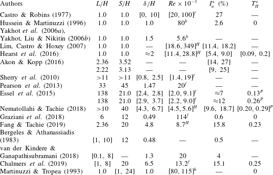
Summary of pertinent previous studies on flows over bluff bodies. The Reynolds numbers with superscripts
 $(\cdot )^{b}$
,
 $(\cdot )^{H}$
and
 $(\cdot )^{f}$
are defined using the upstream bulk mean velocity,
 $U_{H}$
and
 $U_{\infty }$
/upstream maximum mean velocity, respectively, as well as the body height
 $H$
. Symbol — denotes a parameter that is unavailable from the reference. The values with superscript
 $(\cdot )^{P}$
are obtained through private communication. Note that
 $I_{u}^{\ast }$
and
 $T_{H}^{\ast }$
are non-dimensionalized using
 $H$
and
 $U_{H}$
, i.e.
 $I_{u}^{\ast }=I_{u}/U_{H}$
and
 $T_{H}^{\ast }=T_{H}H/U_{H}$
.

A significant amount of literature has been accumulated on surface-mounted cubes and FFS. Table 1 provides a summary of past investigations of special relevance to the present study. Separated shear layers around cubes placed in a fully developed turbulent channel flow were investigated experimentally (Hussein & Martinuzzi Reference Hussein and Martinuzzi1996) and numerically (Yakhot et al.
Reference Yakhot, Anor, Liu and Nikitin2006a
,Reference Yakhot, Liu and Nikitin
b
), while measurements of the heat transfer characteristics were reported by Meinders et al. (Reference Meinders, Hanjalic and Martinuzzi1999). In spite of significant variation in upstream flow conditions in these studies, differences in the reattachment length and vortex shedding frequencies in the wake region are marginal. The effects of Reynolds number and
 $\unicode[STIX]{x1D6FF}/H$
on flow around surface-mounted cubes were investigated by Castro & Robins (Reference Castro and Robins1977), and more recently by Lim et al. (Reference Lim, Castro and Hoxey2007). The wide range of Reynolds number, turbulence intensity and
 $\unicode[STIX]{x1D6FF}/H$
reported in these latter studies (see table 1) were achieved through a combination of wind tunnel and field measurements, and by controlling the free-stream velocity and body height. These studies demonstrate that the nature of oncoming flow and orientation of the cubes have a strong effect on how the mean flow and turbulent statistics respond to changes in Reynolds number. With oncoming uniform flows, for example, the point of transition to turbulence moved toward the leading edge of the cube as Reynolds number, based on the free-stream velocity and body height, increased up to
 $Re_{\infty }=3\times 10^{4}$
. On the other hand, no distinct Reynolds number effects were observed beyond
 $Re_{H}>4000$
in the case of a thick oncoming TBL with
 $\unicode[STIX]{x1D6FF}/H=10$
.
Hearst et al. (Reference Hearst, Gomit and Ganapathisubramani2016) investigated the influence of upstream turbulence on the wake flow around surface-mounted cubes. The experiments were performed at fixed values of
 $\unicode[STIX]{x1D6FF}/H\approx 2$
and dimensionless mean shear
 $T_{H}^{\ast }\approx 0.1$
, but for different levels of upstream turbulence (
 $I_{u}^{\ast }=6.3\,\%{-}9.0\,\%$
) that were generated using active grids. Measurements were also performed in a canonical TBL with approximately no free-stream turbulence (
 $I_{u}^{\ast }=5.4\,\%$
,
 $T_{H}^{\ast }\approx 0.2$
). Altogether, a sufficient mix of test cases was realized for an independent assessment of the influence of free-stream turbulence and mean shear on the flow dynamics. Distinct vortex shedding was observed in the wake flows behind the cube, but only for
 $I_{u}^{\ast }\leqslant 7.3\,\%$
, and in these cases, the vortex shedding frequency is independent of free-stream turbulence intensity. The reattachment length behind the cube was also independent of upstream conditions; however, higher turbulence level promotes wake recovery. The separated shear layer from the leading edge attached intermittently on top of the cube regardless of the oncoming condition, but the intermittency of reattachment over the top surface increased from 24 % when the cube was submerged in the canonical TBL to 41 %–48 % in the case of the other oncoming TBLs with higher free-stream turbulence levels. The twofold increase in the intermittency was attributed to the much stronger mean shear. The effects of turbulence on separated flow over 3-D surface-mounted bodies (
 $S/H=3.5$
,
 $L/H=2.36$
and
 $S/H=3.1$
,
 $L/H=2.3$
) were also investigated by Akon & Kopp (Reference Akon and Kopp2016). In these investigations, different roughness terrains with and without a barrier were used to generate turbulence levels that span 9 %–27 % (see table 1). They observed a 37 % reduction in the reattachment length on top of the bluff bodies when the upstream turbulence increased from 13 % to 27 %.
Most of the past investigations on FFS have focused on understanding the effects of Reynolds number and initial conditions on the reattachment length and statistical properties of the separation bubble on the step. A fairly complete review of these investigations can be found in recent publications including Essel et al. (Reference Essel, Nematollahi, Thacher and Tachie2015) and Graziani et al. (Reference Graziani, Lippert, Uystepruyst and Keirsbulck2017). Sherry et al. (Reference Sherry, Lo Jacono and Sheridan2010) performed experiments over a range of Reynolds numbers and for 3 different values of relative boundary layer thickness (
 $\unicode[STIX]{x1D6FF}/H\approx 0.83$
, 1.25 and 2.5). Variation of the mean reattachment length with Reynolds number showed two distinct regimes: an initial regime where the reattachment length increased linearly with Reynolds number, followed by a regime in which the reattachment length is nearly independent of Reynolds number. The transition Reynolds number demarcating these two regimes was identified as
 $Re_{\infty }=8500$
regardless of
 $\unicode[STIX]{x1D6FF}/H$
. Essel & Tachie (Reference Essel and Tachie2015) investigated the effects of Reynolds number and upstream roughness on flow separations over FFS in a fully developed turbulent channel flow. The two regimes identified by Sherry et al. (Reference Sherry, Lo Jacono and Sheridan2010) were confirmed for the upstream smooth-wall condition; however, the transition Reynolds number was significantly lower (
 $Re_{\infty }=6380$
) than in the previous study which is likely due to differences in upstream turbulence level and blockage ratio. They showed that upstream roughness reduced the mean reattachment significantly (up to 44 %) owing to higher levels of turbulence and
 $\unicode[STIX]{x1D6FF}/H$
produced by wall roughness in comparison to the upstream smooth-wall condition. A similar conclusion is reached by Nematollahi & Tachie (Reference Nematollahi and Tachie2018) who reported a 21 % to 46 % reduction in reattachment depending on the specific upstream roughness condition.
The unsteady dynamics of the separation bubble upstream of an FFS in an oncoming laminar flow is described in Stüer, Gyr & Kinzelbach (Reference Stüer, Gyr and Kinzelbach1999) and Wilhelm et al. (Reference Wilhelm, Härtel and Kleiser2003). Stüer et al. (Reference Stüer, Gyr and Kinzelbach1999) postulate, based on visual observation, that the main mechanism of the separation bubble is independent of Reynolds number. They showed that fluid entrained into the upstream separation bubble accumulates over the entire bubble span and is transported parallel to the step. Occasionally, the separation bubble grows significantly in size and the accumulated fluid is released in streaks over the step. Pearson et al. (Reference Pearson, Goulart and Ganapathisubramani2013) examined the dynamics of the separation bubble upstream of an FFS submerged in a thick oncoming TBL (
 $\unicode[STIX]{x1D6FF}/H=1.47$
) using a TR-PIV system. They showed that the separation bubble oscillates considerably in size, and the frequency of this quasi-periodic enlargement and shrinkage (or flapping motion) is associated with large-scale motion (Adrian, Meinhart & Tomkins Reference Adrian, Meinhart and Tomkins2000) embedded in the oncoming TBL. By using a conditional averaging based on the area of reverse flow, it was shown that an enlargement of the separation bubble is preceded by impingement of oncoming low velocity region onto the windward face. The characteristics of the upstream separation bubble as well as its interaction with the separation bubble formed on top of an FFS placed in a thin oncoming TBL (
 $\unicode[STIX]{x1D6FF}/H\approx 0.5$
) were recently investigated by Graziani et al. (Reference Graziani, Kerhervé, Martinuzzi and Keirsbulck2018) using a planar PIV and temporally resolved wall-pressure sensors. From the PIV and pressure measurements, time-resolved flow fields were reconstructed using linear stochastic estimation. The dynamics of the upstream separation bubble in this experiment is fundamentally similar to that observed in the submerged case by Pearson et al. (Reference Pearson, Goulart and Ganapathisubramani2013); however, the recurring events of massive recirculation whereby the reverse flow region of the upstream bubble expands significantly and merges with the recirculation region on top of the step are less probable in their oncoming thin TBL. It was observed that the low-frequency dynamics of the separation bubbles upstream and on top of the step is strongly correlated but opposite in phase so that an expansion of the upstream bubble is accompanied by a contraction of the separation bubble over the step. The time delay between these events, identified as
 $2H/U_{\infty }$
, is a manifestation of the influence of the upstream separation bubble on the bubble on top of the step.
In our recent work (Fang & Tachie Reference Fang and Tachie2019), we investigated turbulent separation bubbles over 2-D bluff body with an intermediate streamwise aspect ratio (
 $L/H=2.36$
) submerged in a thick oncoming TBL using a TR-PIV system. For this geometry and oncoming flow conditions (see table 1), three distinct separation bubbles, as shown in figure 1, were formed. Although reattachment of the mean flow occurs on top of the step, the separating shear layer emanating from the leading edge reattached intermittently on the wall behind the body. The separation bubble over the step exhibited a low-frequency flapping motion which was linked to the large-scale motion embedded in the oncoming TBL, and a higher-frequency break-up event attributed to the inherent instability of the separation bubble itself. A strong mutual interaction was evident between the separation bubbles on top of and behind the body; generally, an enlargement of the former is accompanied by an enlargement of the latter, with a time delay of
 $7.6H/U_{H}$
between these recurring events. By using a phase-shifted co-spectrum analysis, it was shown that the separation bubble behind the body exhibit flapping motion with the same frequency as the bubble on top of the body.
Separation bubbles over surface-mounted cubes and FFS are topologically and dynamically different, and their sensitivity to the oncoming flow condition can be markedly different. Remarkably, though, the spatio-temporal dynamics of turbulent separation bubbles over bluff bodies with streamwise aspect ratios intermediate to a cube and an FFS has not yet been studied. To our knowledge, the sole investigation of spanwise aspect ratio in turbulent flow over surface-mounted bluff bodies was the flow visualization and pressure measurements reported by Martinuzzi & Tropea (Reference Martinuzzi and Tropea1993). These experiments were performed in a fully developed turbulent channel flow over square cross-section (
 $L/H=1$
) bluff bodies with spanwise aspect ratios that varied from
 $S/H=1$
to 24. They concluded that the mean flow at the mid-span in the wake region is nominally two-dimensional for
 $S/H\geqslant 6$
, and for bluff bodies with
 $S/H\geqslant 10$
, the flow within the upstream recirculation bubble develops a cellular structure and passes over the obstacle along preferred paths.
In this paper, we present a systematic investigation of bluff bodies with an intermediate streamwise extent (
 $L/H=2.36$
) and different spanwise widths (
 $S/H\in [1,20]$
) submerged in a thick TBL (
 $\unicode[STIX]{x1D6FF}/H=4.8$
). As shown in Fang & Tachie (Reference Fang and Tachie2019) for the present test case of
 $S/H=20$
, this intermediate
 $L/H$
facilitates mean flow reattachment over the top surface and a strong interaction between the separation bubbles over and behind the bluff body. We aim at studying the effects of spanwise aspect ratio on the flow statistics, the dynamics of the shear layers in both the streamwise–vertical and streamwise–spanwise planes, flapping motion of separation bubbles and interaction between the separation bubbles over and behind the bluff bodies.
The remainder of the paper is organized as follows. In § 2, the experimental set-up, including the water channel facility and time-resolved PIV system are provided. In § 3, the experimental data are analysed in terms of turbulence statistics, characteristics of shear layers, vortex shedding motions in the wake region and interaction between different separation bubbles. Finally, § 4 summarizes the major conclusions of this research.
2 Experimental set-up
The present experimental set-up, including the water channel, PIV system and vector processing algorithm is identical to that provided by Fang & Tachie (Reference Fang and Tachie2019). For the sake of completeness, we briefly describe the test facility, test conditions and measurement procedure in the following subsections.
2.1 Test section and test conditions
The experiments were conducted in a recirculating open water channel located in the Turbulence and Hydraulic Engineering Laboratory (THEL) at the University of Manitoba. The streamwise length (
 $l$
), vertical height (
 $h$
) and spanwise width (
 $b$
) of the water channel are 6 m, 0.45 m and 0.6 m, respectively. The top surface of the water channel is open to the atmosphere, and a 30 kW variable-speed drive motor was used to drive the recirculating water.
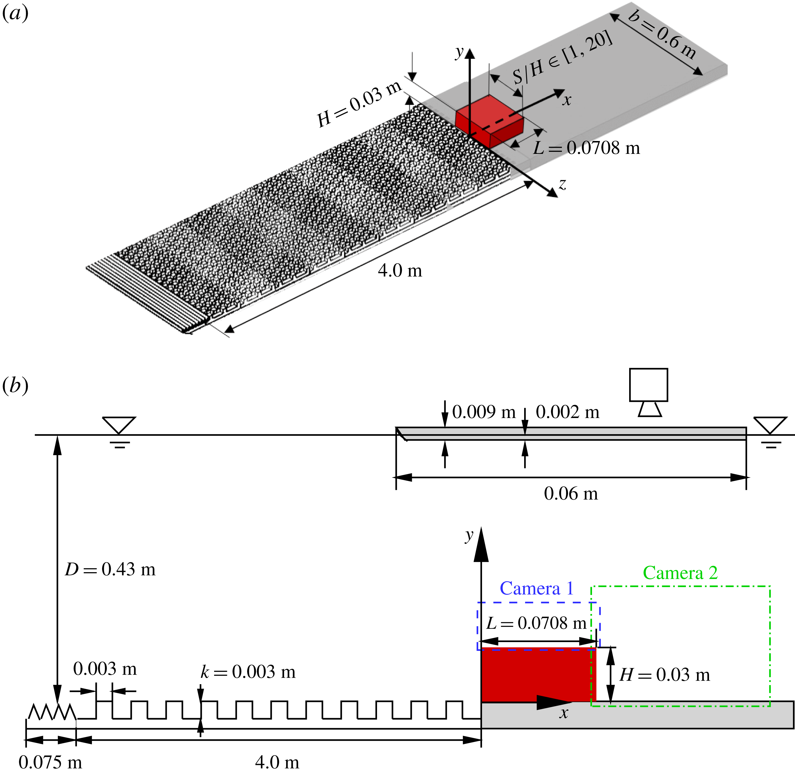
Schematic of test geometry (not to scale) and the adopted coordinate system in (a) the bird’s-eye view and (b) side view, respectively. The spanwise width of the water channel is 0.6 m. The cuboid represents the studied bluff bodies with constant height (
 $H$
), constant length (
 $L$
) and eleven different spanwise widths (
 $S/H=1.0$
, 2.0, 3.0, 3.5, 4.0, 5.0, 6.0, 8.0, 10.0, 12.0 and 20.0). The dashed and dash-dotted rectangular boxes indicate the fields of view of measurement planes
 $S_{xy,a}$
and
 $S_{xy,b}$
, respectively. Note that planes
 $S_{xy,a}$
and
 $S_{xy,b}$
were measured simultaneously.

Figure 2(a) shows the schematic of the test geometry and the adopted coordinate system. The streamwise (
 $x$
), vertical (
 $y$
) and spanwise (
 $z$
) dimensions of the bluff bodies are denoted by
 $L$
,
 $H$
and
 $S$
, respectively. The origin of the
 $x$
coordinate is chosen at the windward face of the body, and the origins of
 $y$
and
 $z$
are set at the bottom wall and channel mid-span, respectively. To generate the desired deep TBL upstream of the bluff bodies, a two-dimensional toothed barrier was mounted at the entrance of the test section, followed by staggered array of cubes. The toothed barrier and the cube-roughened plate span 0.075 m and 4.0 m, respectively, in the streamwise direction and extend across the entire channel width. As shown in figure 2(a), the bluff bodies were mounted over a smooth plate, instead of the cube-roughened plate. The streamwise length and vertical height of the bluff bodies were kept constant at
 $L=0.071~\text{m}$
and
 $H=0.03~\text{m}$
, respectively. A total of eleven spanwise widths corresponding to the following aspect ratios (
 $\mathit{AR}=S/H$
) were tested:
 $\mathit{AR}=1.0$
, 2.0, 3.0, 3.5, 4.0, 5.0, 6.0, 8.0, 10.0, 12.0 and 20.0. In the case of
 $\mathit{AR}=20.0$
, the bluff body spans the entire width of the water channel, and is considered as a 2-D bluff body. The water depth (
 $D$
) and free-stream velocity (
 $U_{\infty }$
) were maintained at 0.43 m and
 $0.41~\text{m}~\text{s}^{-1}$
, respectively, in all the experiments. The room temperature was regulated at
 $20\,^{\circ }\text{C}$
, and therefore, the kinematic viscosity of water (
 $\unicode[STIX]{x1D708}$
) was maintained at
 $10^{-6}~\text{m}^{2}~\text{s}^{-1}$
. The Reynolds number based on the free-stream velocity and body height (
 $Re_{\infty }=U_{\infty }H/\unicode[STIX]{x1D708}$
) was 12 300. Meanwhile, the Froude number based on free-stream velocity and water depth (
 $U_{\infty }/\sqrt{gD}$
, where
 $g=9.81~\text{m}~\text{s}^{-2}$
is the gravitational acceleration) was 0.20, and not surprisingly, no distinct free surface wave was observed. The blockage ratio, which is defined as the ratio between the frontal areas of the bluff bodies (
 $S\times H$
) and the cross-stream area of the water column (
 $b\times D$
), is 7.0 % for the 2-D bluff body and 0.3 %–4.0 % for the cases of
 $\mathit{AR}\in [1,12]$
. Unlike wind tunnel experiments in which boundary layers develop on all four walls, the free surface of the open water channel is equivalent to a symmetry plane. As such, the effective blockage ratio of the bluff bodies varies from 0.15 % for
 $\mathit{AR}=1$
to 3.5 % for
 $\mathit{AR}=20$
. These effective blockage ratios are smaller than the threshold of 5 % below which blockage effect on the flow dynamics is negligible (Farell et al.
Reference Farell, Carrasquel, Güven and Patel1977).
2.2 Time-resolved particle image velocimetry system
A planar TR-PIV system was employed to measure the velocity fields upstream of, over and behind the bluff bodies. The seeding particles were
 $10~\unicode[STIX]{x03BC}\text{m}$
silver coated hollow glass spheres, and the specific gravity was 1.4. As indicated by Fang & Tachie (Reference Fang and Tachie2019), the slip velocity and Stokes number of the seeding particles were
 $2.18\times 10^{-5}~\text{m}~\text{s}^{-1}$
and 0.0014, respectively. As such, these seeding particles are presumed to follow the fluid motions very well, and their instantaneous velocities are a true reflection of the fluid velocities. A diode pumped dual-cavity dual-head high speed Neodymium-doped yttrium lithium fluoride (Nd:YLF) laser supplied by Photonics Industries International, Inc. was used to illuminate the flow field. The wavelength of the laser was 527 nm, and the maximum pulse energy was
 $30~\text{mJ}~\text{pulse}^{-1}$
at a frequency of 1000 Hz. Two 12-bit complementary metal oxide semiconductor (CMOS) cameras were used to image the light scattered by the illuminated particles. The full resolution of the CMOS cameras was
 $2560~\text{pixel}\times 1600~\text{pixel}$
at an acquisition frequency of 807 Hz.
Parameters and notations of the measurement planes. Planes
 $U_{1}$
and
 $U_{2}$
were measured without installing the bluff bodies. 12 000 and 6000 samples were collected in planes
 $U_{1}$
and
 $U_{2}$
. For the bluff bodies of
 $S/H=2.0$
, 3.0, 4.0, 5.0, 6.0, 10.0 and 12.0, 8000 samples were collected for planes
 $S_{xy,a}$
and
 $S_{xy,b}$
, and no measurement was performed in plane
 $S_{xz}$
. As for the bluff bodies of
 $S/H=1.0$
, 3.5, 8.0 and 20.0, 32 000 samples were collected in planes
 $S_{xy,a}$
and
 $S_{xy,b}$
, and 36 000 samples were collected in plane
 $S_{xz}$
for the bluff bodies of
 $S/H=1.0$
, 3.5 and 8.0.

Table 2 lists the parameters and notations of the measurement planes. Specifically, the upstream TBL was measured without installing the bluff bodies first in plane
 $U_{1}$
using a single-frame (time-resolved) mode and subsequently in plane
 $U_{2}$
using a double-frame mode. The field of view of plane
 $U_{1}$
was large enough to cover the entire thickness of the oncoming TBL (
 $y/H\in [-0.3,7.0]$
), whereas the field of view of plane
 $U_{2}$
was reduced to achieve a better spatial resolution of the flow statistics in the lower boundary layer region (
 $y/H\in [-0.1,3.2]$
). Subsequently, the bluff bodies were installed and measurements were conducted in two planes
 $S_{xy,a}$
and
 $S_{xy,b}$
at the mid-span. As shown in figure 2(b), planes
 $S_{xy,a}$
and
 $S_{xy,b}$
measure the flow fields over and behind the bluff bodies, respectively, and the measurements in planes
 $S_{xy,a}$
and
 $S_{xy,b}$
were always performed simultaneously. For all the
 $x$
–
 $y$
plane measurements (
 $U_{1}$
,
 $U_{2}$
,
 $S_{xy,a}$
and
 $S_{xy,b}$
), the laser was positioned above the water channel, shooting vertically down through the free surface, and the camera was positioned perpendicular to the side walls of the water channel. For the bluff bodies with
 $\mathit{AR}=2.0$
, 3.0, 4.0, 5.0, 6.0, 10.0 and 12.0, 8000 samples were collected in these
 $x$
–
 $y$
planes, and were deemed sufficient to ensure statistical convergence of the mean flow over and behind the bluff bodies. As will become apparent subsequently, the bluff bodies with
 $\mathit{AR}=1.0$
and 3.5 exhibit characteristics typical of a 3-D configuration,
 $\mathit{AR}=20$
represents a 2-D configuration, and
 $\mathit{AR}=8$
shows features intermediate to 2-D and 3-D bluff bodies. To facilitate detailed analysis that encompasses 3-D, transitional and 2-D bluff bodies, 32 000 samples were collected in planes
 $S_{xy,a}$
and
 $S_{xy,b}$
for the bluff bodies with
 $\mathit{AR}=1.0$
, 3.5, 8.0 and 20.0. Detailed measurements were also made in the
 $x$
–
 $z$
plane
 $S_{xz}$
at half-body height in the wake region behind the bluff bodies with
 $\mathit{AR}=1.0$
, 3.5 and 8.0, and for these measurements, 36 000 samples were collected. As shown in figure 2, the high-speed camera was positioned above the free surface for these
 $x$
–
 $z$
plane measurements. A precursor measurement showed that the particle images were smeared by minute surface ripples and therefore the quality of velocity vectors was severely degraded. To resolve this problem, a 9 mm thick acrylic plate was submerged 2 mm into the water and covered the field of view of plane
 $S_{xz}$
(see figure 2
b). The leading edge of this plate was also rounded to minimize the influence on the flows developed over the bottom wall.
To better resolve the strong shear layer and the associated vortical structures emanating from the leading edge, a Sigma 105 mm macro lens was used to image flow field in plane
 $S_{xy,a}$
, while a Nikon 60 mm lens was employed for all other measurement planes. The sampling frequency for the measurement planes
 $U_{1}$
,
 $S_{xy,a}$
and
 $S_{xy,b}$
was 1000 Hz, which corresponds to 2.3 wall units, i.e.
 $f^{+}=f\unicode[STIX]{x1D708}/u_{\unicode[STIX]{x1D70F}}^{2}=2.3$
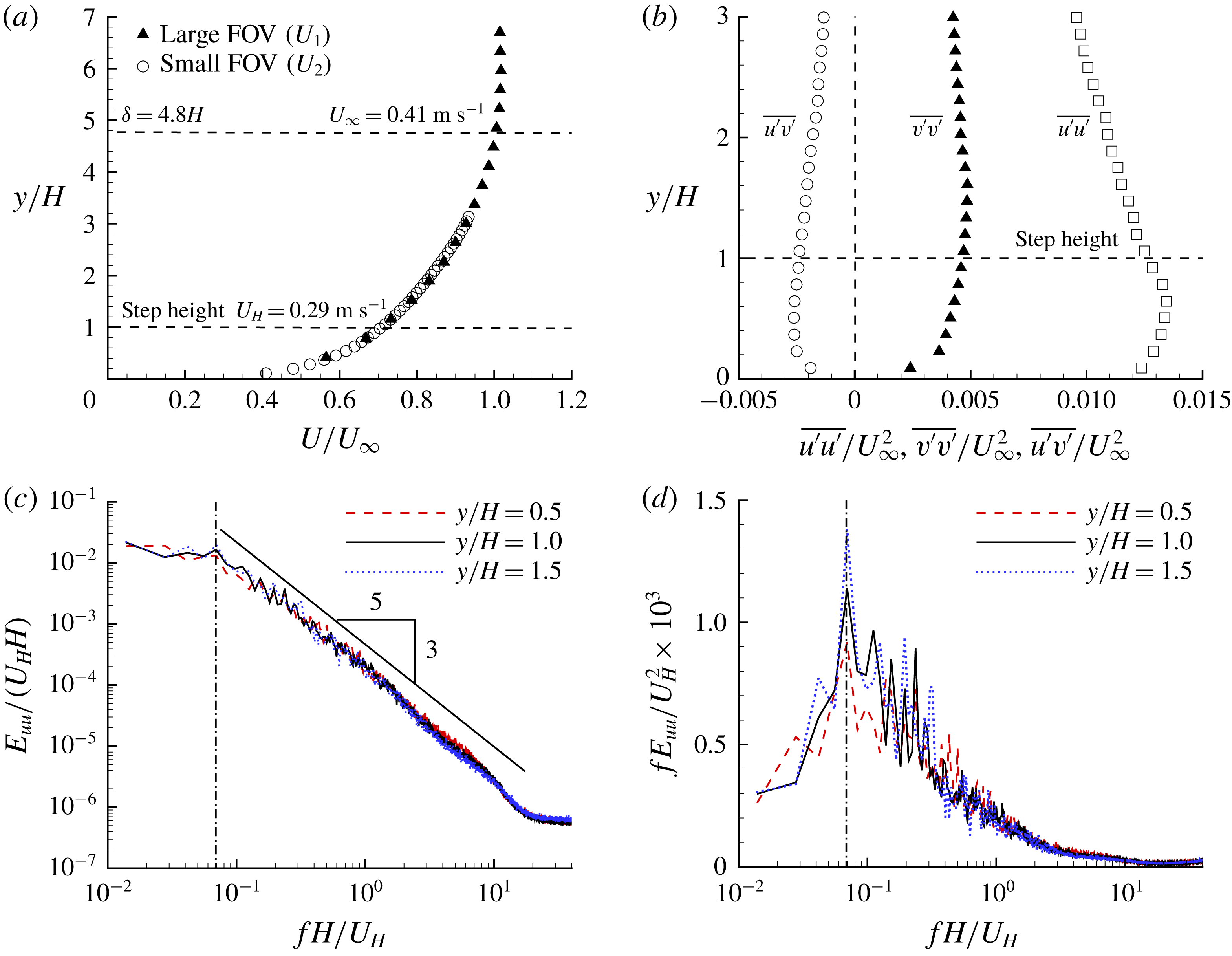
. As will be shown in figure 3(c), negligible energy is held around this sampling frequency. Therefore, the sampling frequency used in this research is deemed to be sufficient to resolve all significant temporal scales of the studied turbulent flows. Measurements in plane
 $S_{xz}$
were performed at a sampling frequency of 807 Hz and the full resolution of the camera was used in this case.
The commercial software DaVis 8.4 supplied by LaVision Inc. was used for both data acquisition and vector processing. A GPU-accelerated multi-pass cross-correlation algorithm was used to calculate the velocity vectors. The interrogation areas reduce from
 $128~\text{pixel}\times 128~\text{pixel}$
(50 % overlap) at the initial pass to
 $32~\text{pixel}\times 32~\text{pixel}$
(75 % overlap) at the final pass.
In this paper, the Reynolds decomposition is employed such that the instantaneous velocity is decomposed as
 $u=\overline{u}+u^{\prime }$
, where
 $\overline{(\cdot )}$
and
 $(\cdot )^{\prime }$
denote the time-averaged and fluctuation components, respectively. For convenience, the mean velocity is denoted by an upper case, e.g.
 $U\equiv \overline{u}$
. For conciseness in the discussion, a notion AR20 is used to denote the bluff body with an aspect ratio of 20, and so on for all other bluff bodies.
3 Results and discussion
3.1 Oncoming flow condition
Characterization of the oncoming turbulent boundary layer. (a,b) The vertical profiles of streamwise mean velocity (
 $U$
) and Reynolds stresses (
 $\overline{u^{\prime }v^{\prime }}$
,
 $\overline{u^{\prime }u^{\prime }}$
and
 $\overline{v^{\prime }v^{\prime }}$
), respectively. Every fifth measurement point is plotted for clarity. (c,d) The frequency spectra of streamwise velocity (
 $E_{uu}$
) at three different elevations in logarithmic and premultiplied scales, respectively. The vertical dash-dotted lines mark the frequency of
 $St=fH/U_{H}=0.069$
.

Summary of the test parameters.

To characterize the oncoming TBL, figure 3 shows the streamwise mean velocity (
 $U$
), Reynolds stresses (
 $\overline{u^{\prime }v^{\prime }}$
,
 $\overline{u^{\prime }u^{\prime }}$
and
 $\overline{v^{\prime }v^{\prime }}$
) and frequency spectra of the streamwise velocity (
 $E_{uu}$
) measured in planes
 $U_{1}$
and
 $U_{2}$
(see table 2) without installing the bluff bodies. Table 3 summarizes the pertinent test parameters of the present study. The boundary layer thickness
 $\unicode[STIX]{x1D6FF}$
, defined as the vertical distance from the wall to the point where
 $U=0.99U_{\infty }$
, is 144 mm, i.e.
 $\unicode[STIX]{x1D6FF}=4.8H$
, which is much thicker than the step height. The dimensionless mean shear at the body height (
 $T_{H}^{\ast }$
) is calculated to be 0.23. Following Flack, Schultz & Shapiro (Reference Flack, Schultz and Shapiro2005) and Wu & Christensen (Reference Wu and Christensen2007), the friction velocity (
 $U_{\unicode[STIX]{x1D70F}}$
) is estimated using the total shear stress method (i.e.
 $U_{\unicode[STIX]{x1D70F}}\approx (\unicode[STIX]{x1D708}\unicode[STIX]{x2202}U/\unicode[STIX]{x2202}y-\overline{u^{\prime }v^{\prime }})_{max}^{1/2}$
) as
 $0.021~\text{m}~\text{s}^{-1}$
. As such, the Reynolds number based on the friction velocity
 $Re_{\unicode[STIX]{x1D70F}}=\unicode[STIX]{x1D6FF}U_{\unicode[STIX]{x1D70F}}/\unicode[STIX]{x1D708}$
is 3000. The body height is
 $H^{+}=630$
, where the superscript
 $(\cdot )^{+}$
denotes non-dimensionalization using
 $U_{\unicode[STIX]{x1D70F}}$
and
 $\unicode[STIX]{x1D708}$
, and extends well into the log layer. As seen in figure 3(c), the frequency spectra
 $E_{uu}$
exhibit an inertial subrange featuring the famous
 $-5/3$
slope (Pope Reference Pope2000) in the range of
 $St=fH/U_{H}\in [0.1,10]$
. In this paper, unless otherwise stated, the Strouhal number is defined as
 $St=fH/U_{H}$
following prior studies with thick oncoming TBLs (Lim et al.
Reference Lim, Castro and Hoxey2007; Hearst et al.
Reference Hearst, Gomit and Ganapathisubramani2016; Fang & Tachie Reference Fang and Tachie2019). Lim et al. (Reference Lim, Castro and Hoxey2007) also showed an inertial subrange within
 $St\in [0.1,10]$
at Reynolds numbers which are an order of magnitude higher than in the present study. This similarity reflects the universality of the inertial subrange in high Reynolds number TBLs. Figure 3(d) shows that the streamwise velocity in the vicinity of the step height possesses a dominant frequency at
 $St=0.069$
. For the turbulence structures associated with this peak frequency, if the convective velocity is estimated as
 $U_{H}$
(
 $0.71U_{\infty }$
), the characteristic streamwise length of the structures is approximately
 $3\unicode[STIX]{x1D6FF}$
. This value is in good agreement with the typical length scale of
 $2{-}3\unicode[STIX]{x1D6FF}$
for the lager-scale motion (LSM) in the outer region of the TBL at high Reynolds numbers (Adrian et al.
Reference Adrian, Meinhart and Tomkins2000; Tomkins & Adrian Reference Tomkins and Adrian2003; Monty et al.
Reference Monty, Hutchins, Ng, Marusic and Chong2009). The LSM is induced by packets of streamwise aligned hairpin structures and features alternating positive and negative streamwise fluctuating velocities.
From tables 1 and 3, it is noted that the present values of
 $\unicode[STIX]{x1D6FF}/H$
,
 $I_{u}^{\ast }$
and
 $T_{H}^{\ast }$
are one of the highest combinations examined to date. This thick TBL is advantageous in terms of generating an oncoming flow condition to mimic the realistic atmospheric boundary layer, which features both strong mean shear and high-level turbulence intensity. Indeed, the present high level of turbulence intensity is close to the atmospheric boundary layer condition in the field measurements by Lim et al. (Reference Lim, Castro and Hoxey2007). Morrison & Kopp (Reference Morrison and Kopp2018) also performed field measurement around a low-rise building submerged in atmospheric boundary layer with an oncoming turbulence intensity 18.6 %, which is comparable to the present value of 15.8 %.
3.2 Mean flow and reattachment lengths
Contours of streamwise mean velocity (
 $U$
) and mean streamlines over the step in selected four different aspect ratio (
 $AR$
) cases. The dashed isopleths is
 $\unicode[STIX]{x1D6F9}(y)=\int _{wall}^{y}U\,\text{d}Y=0$
. The dash–dot–dotted and dash–dotted isopleths are forward flow fraction (
 $\unicode[STIX]{x1D6FE}$
) at 0.95 and 0.5, respectively.

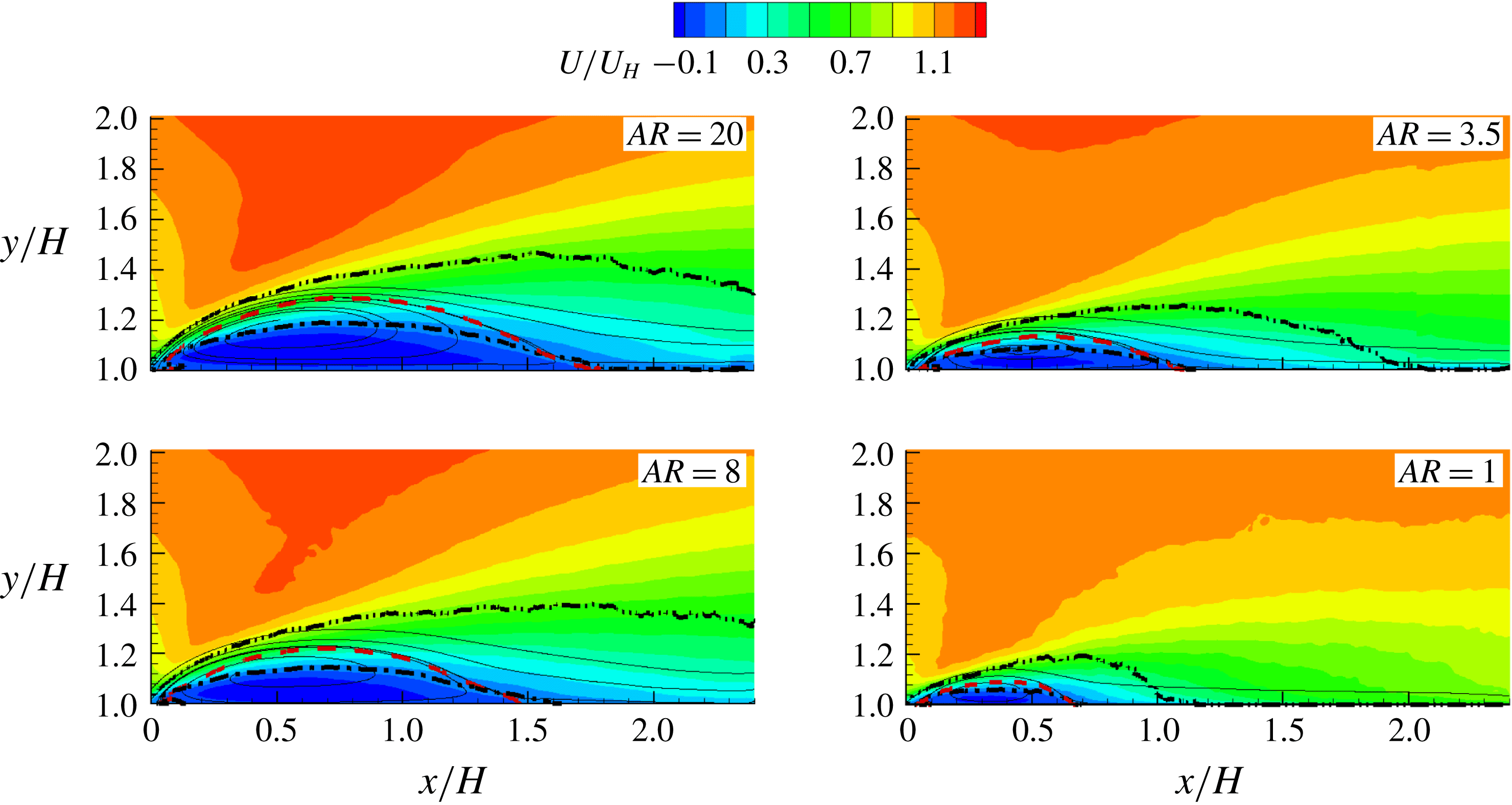
Figure 4 shows contours of the streamwise mean velocity (
 $U$
) and mean streamlines over the bluff bodies in the mid-span plane for selected
 $AR$
cases. For the range of
 $AR$
(
 $\mathit{AR}\in [1,20]$
) examined, the mean flow separates at the leading edge and reattaches over the bluff body. Hereinafter, the turbulent separation bubble over the step is represented by TSBA for conciseness. From the figure, the isopleths of 50 % forward flow fraction (
 $\unicode[STIX]{x1D6FE}=0.5$
) emanate from the leading edge, pass through the foci of TSBA, and terminate on top of the bluff bodies. The isopleths of
 $\unicode[STIX]{x1D6F9}\equiv \int _{wall}^{y}U\,\text{d}Y=0$
are close to the separating streamlines, forming the upper bound of TSBA. Regardless of the aspect ratio, the separating streamline and isopleths of
 $\unicode[STIX]{x1D6FE}=0.5$
and
 $\unicode[STIX]{x1D6F9}=0$
intersect with the top of the bluff body at the same point, which is defined as the reattachment point. It is evident from the figures that the size, both vertical and streamwise extents, of the mean separation bubble grows monotonically as
 $AR$
increases. Furthermore, the isopleths of
 $\unicode[STIX]{x1D6FE}=0.95$
extend beyond the top surface in the AR20 and AR8 cases, but terminate prior to the trailing edge in the AR3.5 and AR1 cases. This indicates that instantaneous flow reattachment over the top surface occurs intermittently in the AR20 and AR8 cases but permanently in the AR3.5 and AR1 cases.
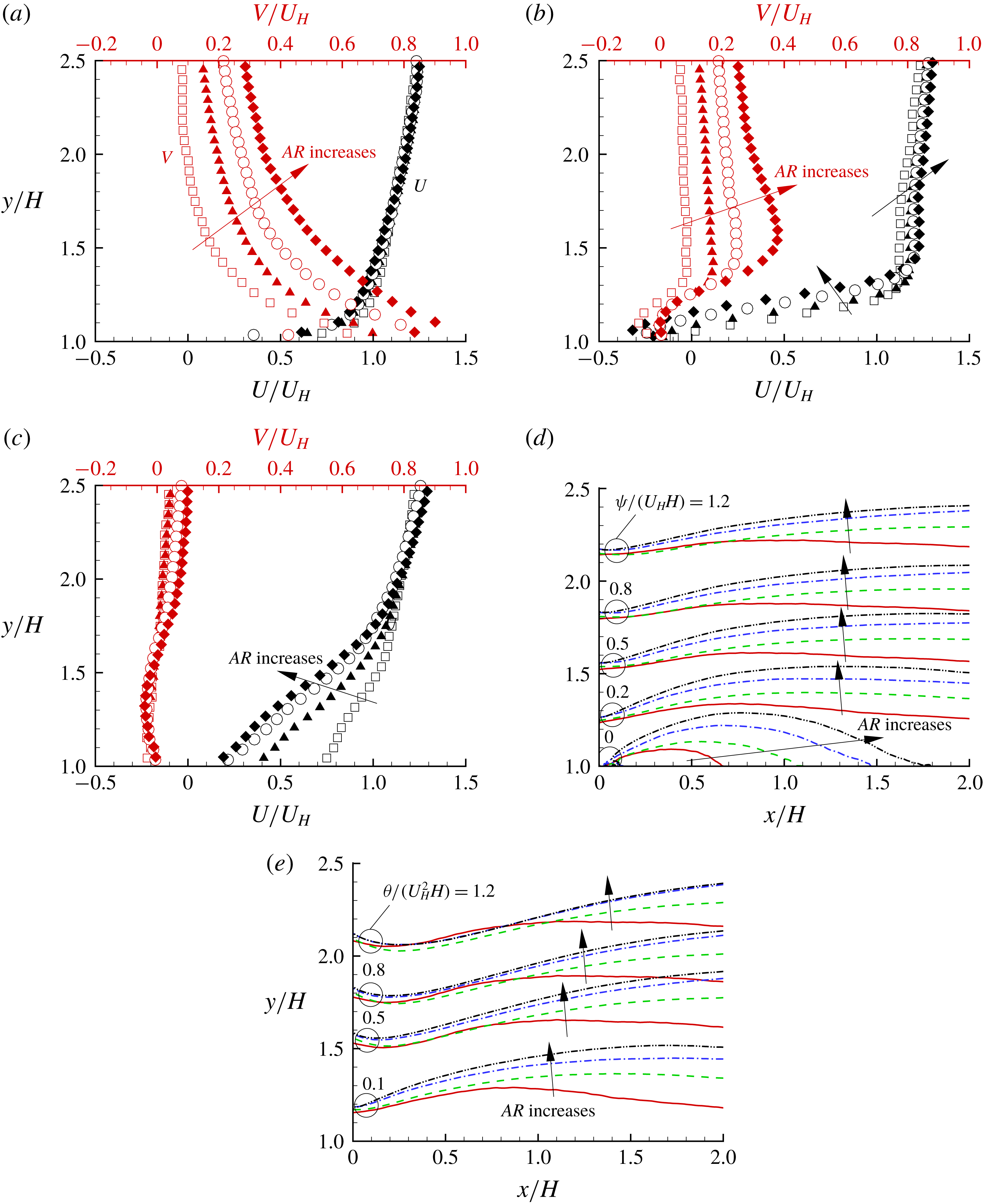
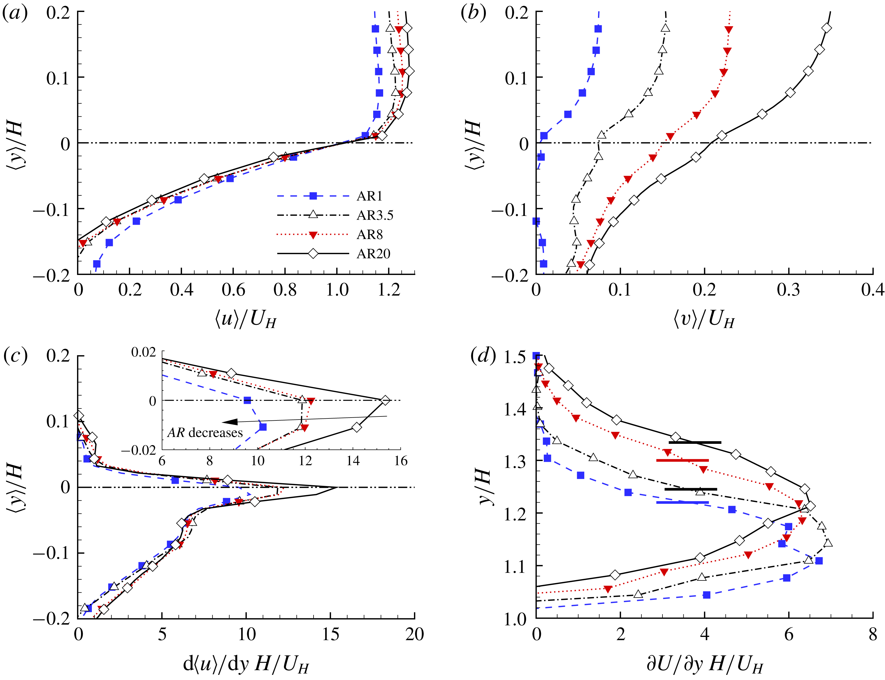
Vertical profiles of
 $U$
and
 $V$
at
 $x/H=0$
(a), 0.5 (b) and 2.2 (c) in the AR1 (hollow squares), AR3.5 (solid triangles), AR8 (hollow circles) and AR20 (solid diamonds) cases. Isopleths of (d)
 $\unicode[STIX]{x1D6F9}$
and (e)
 $\unicode[STIX]{x1D6E9}$
in the AR1 (solid), AR3.5 (dashed), AR8 (dash-dotted) and AR20 (black dash–dot–dot) cases. The bundles of isopleths at the same levels (indicated by the number by side) are marked by circles. The arrows mark the monotonic variation as
 $AR$
increases.

The development of mean flow over the bluff bodies is further examined using the vertical profiles of mean velocities (
 $U$
and
 $V$
) and isopleths of
 $\unicode[STIX]{x1D6F9}$
and
 $\unicode[STIX]{x1D6E9}$
, where
 $\unicode[STIX]{x1D6E9}(y)\equiv \int _{wall}^{y}U^{2}\,\text{d}Y$
. The latter two parameters (
 $\unicode[STIX]{x1D6F9}$
and
 $\unicode[STIX]{x1D6E9}$
) provide a measure of the streamwise mass and momentum flow fluxes, respectively, below the elevation of
 $y$
. As shown in figure 5(a), at the leading edge, the vertical profiles of
 $U$
are almost identical in all the cases; however, the vertical flow motions increase monotonically as
 $AR$
increases. As such, as
 $AR$
increases the flow angle (defined as
 $\arctan (V/U)$
) at the leading edge increases and as a consequence, the size of mean separation bubble increases. Prior to the reattachment point (figure 5
b), the magnitude of reverse flow increases with
 $AR$
and due to the constraint of continuity, the stronger velocity deficit near the wall in the case of larger
 $AR$
is compensated for by a larger
 $U$
away from the wall. From figure 5(c), the stronger velocity deficit near the wall induced by the larger separation bubble causes a slower recovery to a canonical TBL. As seen in figures 5(d) and 5(e), the vertical distributions of
 $\unicode[STIX]{x1D6F9}$
and
 $\unicode[STIX]{x1D6E9}$
are similar at the leading edge in different cases, but decrease monotonically with increasing
 $AR$
at any downstream location. Thus, larger mass and momentum deficits are generated in the near-wall region over bluff bodies of larger
 $AR$
, and as such, both the displacement and momentum thicknesses over the bluff bodies increase as
 $AR$
increases.
(a) Contours of streamwise mean velocity
 $U$
superimposed with mean streamlines, dash-dot isopleth of forward flow fraction (
 $\unicode[STIX]{x1D6FE}$
) at 0.5 and dashed isopleth of
 $\unicode[STIX]{x1D6F9}(y)=\int _{wall}^{y}U\,\text{d}Y=0$
behind the step for four different
 $AR$
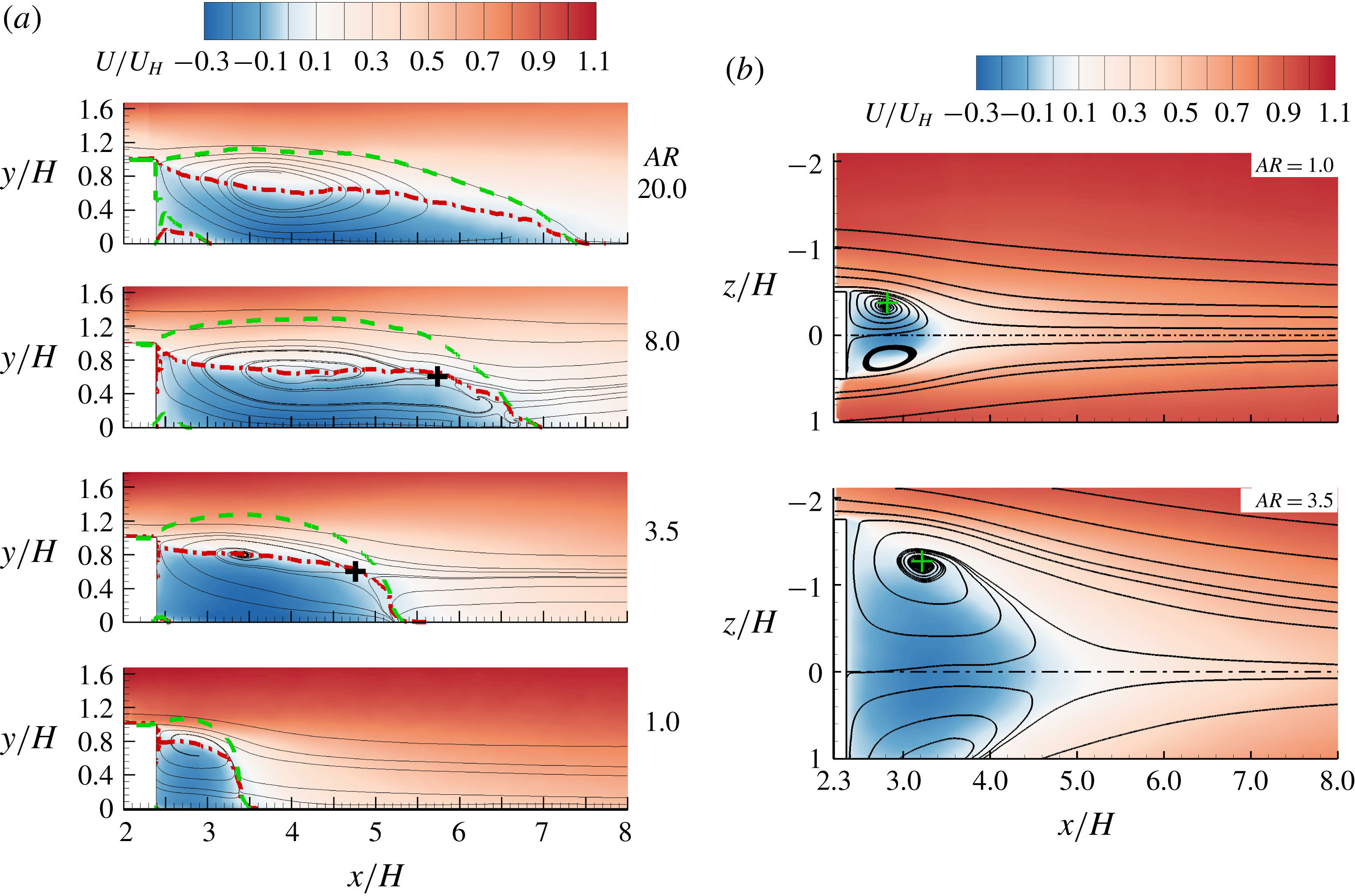
cases. The cross symbols mark the saddle points. (b) Mean flow in the
 $x$
–
 $z$
plane at half-step height (
 $y/H=0.5$
). The dash-dotted lines mark the spanwise locations of mid-span. The cross symbols mark the foci of mean recirculation region.

Figure 6(a) shows the mean flow fields in the mid-span behind the bluff bodies. The separation bubble behind the bluff body is hereafter denoted as TSBB for conciseness. Similar to TSBA, the streamwise extent of TSBB increases monotonically as
 $AR$
increases. However, the topology of the mean streamlines is sensitive to
 $AR$
. For instance, in the AR3.5 case, distinct mean streamlines emanate from the reattachment point on the bottom wall (around
 $x/H=5.3$
) and form a pattern of a half-nodal point. Additional saddles (as marked by crosses
 $+$
), generated by the clashing of upwash flow from the bottom wall and downwash flow from the top, can be observed in the AR3.5 and AR8 cases. Wang et al. (Reference Wang, Zhou, Chan and Lam2006) and Wang & Zhou (Reference Wang and Zhou2009) also observed such saddles in the wake flow behind finite-length circular and square cylinders (
 $AR\leqslant 0.2$
). They attributed the upwash flow to the base vortex, a pair of streamwise counter-rotating vortices near the base of bluff bodies. They also observed that a thicker TBL led to enhanced base vortex. It appears in the literature that a base vortex does not occur around a cube, and is only observed in bluff bodies with small values of
 $AR$
(Hunt et al.
Reference Hunt, Abell, Peterka and Woo1978; Hussein & Martinuzzi Reference Hussein and Martinuzzi1996; Wang et al.
Reference Wang, Zhou, Chan and Lam2006; Wang & Zhou Reference Wang and Zhou2009). This is consistent with the observation in our AR1 case, where no upwash flow is observed behind the step, but inconsistent with the existence of upwash flow in the AR3.5 and AR8 cases for which a pair of base vortices is formed. It is also interesting to note that two foci can be seen behind the step in the AR8 case.
Figure 6(b) shows the mean flow in the
 $x$
–
 $z$
plane at half-body height (
 $y/H=0.5$
) in the AR1 and AR3.5 cases. The counterpart plot in the AR8 case is qualitatively similar to the plotted two cases, and is thus not shown here. Evidently, a distinct recirculation motion occurs in the wake region near the spanwise ends of the bluff bodies. In the AR1 case, the distance between the vortex core and mid-span is approximately
 $0.38H$
. This distance is identical to that observed by Yakhot et al. (Reference Yakhot, Liu and Nikitin2006b
) in the wake flow behind a cube. In addition, the vertical location of the vortex core in the mid-span behind the bluff body of
 $\mathit{AR}=1$
(see figure 6
a) is at
 $y/H=0.8$
, which is also very similar to that in the wake of a cube observed by Yakhot et al. (Reference Yakhot, Liu and Nikitin2006b
) and Hearst et al. (Reference Hearst, Gomit and Ganapathisubramani2016). It is therefore expected that an arch-shaped vortex occurs in the wake region in the AR1 case, as commonly observed in the wake flow of cubes (Hunt et al.
Reference Hunt, Abell, Peterka and Woo1978; Martinuzzi & Tropea Reference Martinuzzi and Tropea1993; Hussein & Martinuzzi Reference Hussein and Martinuzzi1996; Krajnović & Davidson Reference Krajnović and Davidson2002; Yakhot et al.
Reference Yakhot, Liu and Nikitin2006b
). As
 $AR$
increases, the vortex core moves farther away from the mid-span. This is consistent with the observation made by Martinuzzi & Tropea (Reference Martinuzzi and Tropea1993) using an oil film on the bottom wall. Specifically, the vortex cores at
 $y/H=0.5$
in the AR1, AR3.5 and AR8 cases occur at
 $z/H=0.38$
, 1.24 and 2.14, respectively. These spanwise locations are, respectively,
 $0.12H$
,
 $0.51H$
and
 $1.86H$
away from the vertical tips of the bluff bodies in the spanwise direction.
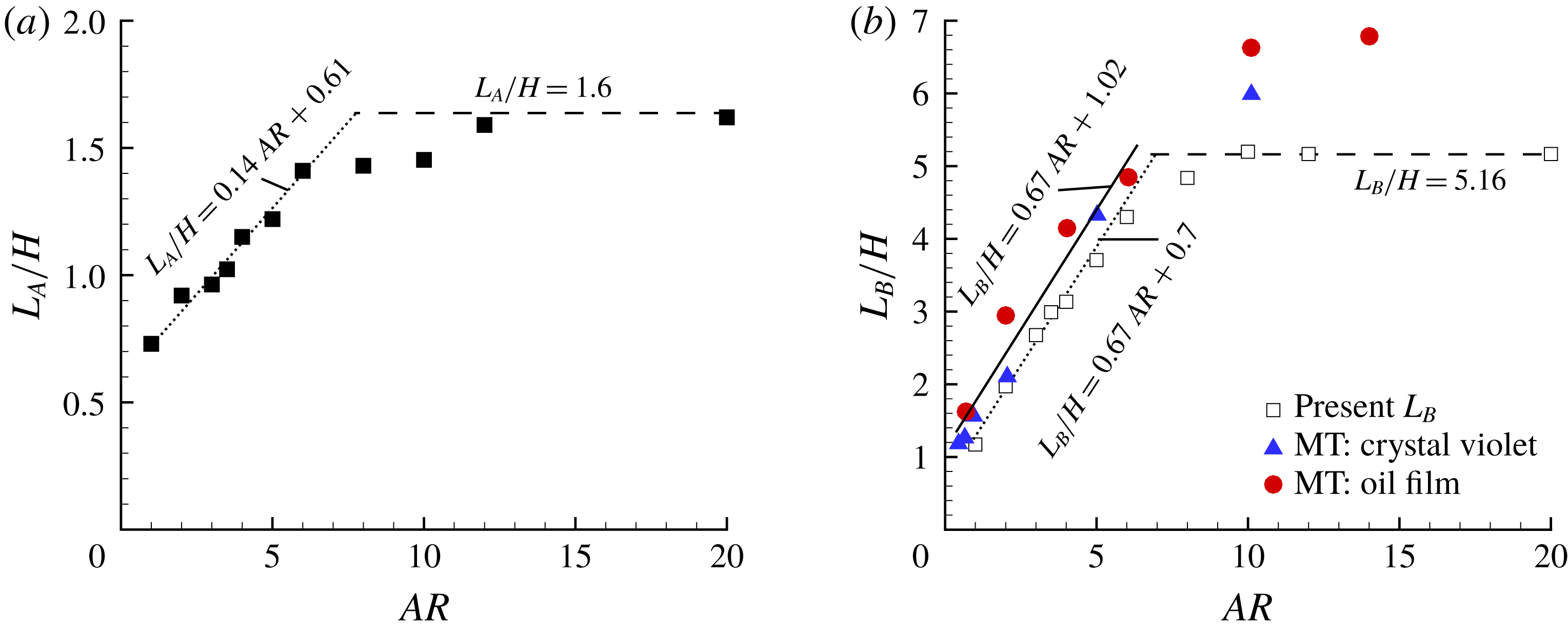
(a) Variation of reattachment lengths over the step (
 $L_{A}$
) with
 $AR$
. (b) Variation of reattachment lengths behind the step (
 $L_{B}$
) with
 $AR$
.
 $L_{B}$
is defined as the distance between the leeward face of the step to the reattachment point. In (a,b), a linear equation (dotted lines) is fitted for
 $\mathit{AR}\in [1,6]$
using a least-squares-error method. In (b), the points plotted using solid symbols are measurement data by Martinuzzi & Tropea (Reference Martinuzzi and Tropea1993) using two methods (crystal violet and oil film). The solid straight line indicates the fitted linear function by Martinuzzi & Tropea (Reference Martinuzzi and Tropea1993).

Figure 7 shows the variation of the reattachment lengths over the bluff bodies (
 $L_{A}$
) and behind the bluff bodies (
 $L_{B}$
) with
 $AR$
. In general, both
 $L_{A}$
and
 $L_{B}$
increase monotonically as
 $AR$
increases, and reach asymptotic values for sufficiently large
 $AR$
. There exist three distinct regimes of
 $AR$
: (i) a 3-D regime featuring a linear variation of
 $L_{A}$
and
 $L_{B}$
with
 $AR$
; (ii) a 2-D regime featuring constant values of
 $L_{A}$
and
 $L_{B}$
; and (iii) a transition regime between the 3-D and 2-D regimes. The 3-D regimes for
 $L_{A}$
and
 $L_{B}$
are identically within
 $1\leqslant \mathit{AR}\leqslant 6$
, whereas the 2-D regimes for
 $L_{A}$
and
 $L_{B}$
are for
 $\mathit{AR}\geqslant 12$
and
 $\mathit{AR}\geqslant 10$
, respectively. The present results support the recommendation by De Brederode & Bradshaw (Reference De Brederode and Bradshaw1972) and Kiya & Sasaki (Reference Kiya and Sasaki1983) that bluff bodies with
 $AR$
larger than 10 are necessary to generate nominally two-dimensional flow in the mid-span. The above results provide the premise for our choice of AR1 and AR3.5 as 3-D configurations, AR8 as a transitional configuration and AR20 as a 2-D configuration to represent all three different regimes.
Figure 7 also reveals that even though both
 $L_{A}$
and
 $L_{B}$
vary linearly with
 $AR$
in the 3-D regime (i.e.
 $\mathit{AR}\in [1,6]$
), the slope
 $\text{d}(L_{B}/H)/\text{d}\mathit{AR}=0.67$
is more than four times as large as
 $\text{d}(L_{A}/H)/\text{d}\mathit{AR}$
, indicating that TSBB is more sensitive to changes in
 $AR$
than TSBA. The fitted line to the experimental data by Martinuzzi & Tropea (Reference Martinuzzi and Tropea1993) possesses an identical slope as in the present study. However, the asymptotic values of
 $L_{B}$
in the previous study are significantly larger than the present results. As summarized in tables 1 and 3, the characteristics of the oncoming TBL are drastically different between Martinuzzi & Tropea (Reference Martinuzzi and Tropea1993) and the present study. Based on these observations, we conclude that
 $L_{B}$
for large
 $AR$
or a nominally 2-D case is sensitive to the oncoming flow condition. In contrast,
 $L_{B}$
for small
 $AR$
or a 3-D case is insensitive to the oncoming flow condition. Hearst et al. (Reference Hearst, Gomit and Ganapathisubramani2016) also concluded that the reattachment length behind a surface-mounted cube is independent of the oncoming turbulence intensity or mean shear.
In contrast to the aforementioned insensitivity of
 $L_{B}$
in the 3-D regime to the oncoming flow condition,
 $L_{A}$
is strongly dependent on the oncoming flow condition in both the 3-D and 2-D regimes. Indeed, the available literature show that the reattachment length over an FFS (2-D regime) varies from
 $1.2H$
(Essel & Tachie Reference Essel and Tachie2015) to
 $4.7H$
(Moss & Baker Reference Moss and Baker1980) depending on the oncoming flow condition. Nematollahi & Tachie (Reference Nematollahi and Tachie2018) also observed that the reattachment length over an FFS decreased from
 $2.27H$
to
 $1.23H$
as the upstream wall condition was changed from smooth to rough. Akon & Kopp (Reference Akon and Kopp2016) showed that the reattachment length over a 3-D bluff body with
 $L/H=2.36$
and
 $S/H=3.5$
, which is identical to the present AR3.5 case, decreases from
 $1.4H$
to
 $0.88H$
as the oncoming turbulence intensity (
 $I_{u}^{\ast }$
) increases from 13 % to 27 %. It is also noted here that for an intermediate turbulence intensity of
 $I_{u}^{\ast }=17\,\%$
(which is not significantly different from the present 15.8 %), Akon & Kopp (Reference Akon and Kopp2016) observed the same value of
 $L_{A}$
as the present study (at
 $1.0H$
). Additionally, the reattachment length over the bluff body with
 $\mathit{AR}=1$
in the present study is approximately
 $0.73H$
, a value that is 27 % smaller than
 $H$
. This is at variance with the common observation that full reattachment does not occur on top of a cube (i.e.
 $L_{A}>H$
) (Castro & Robins Reference Castro and Robins1977; Yakhot et al.
Reference Yakhot, Liu and Nikitin2006b
; Hearst et al.
Reference Hearst, Gomit and Ganapathisubramani2016).
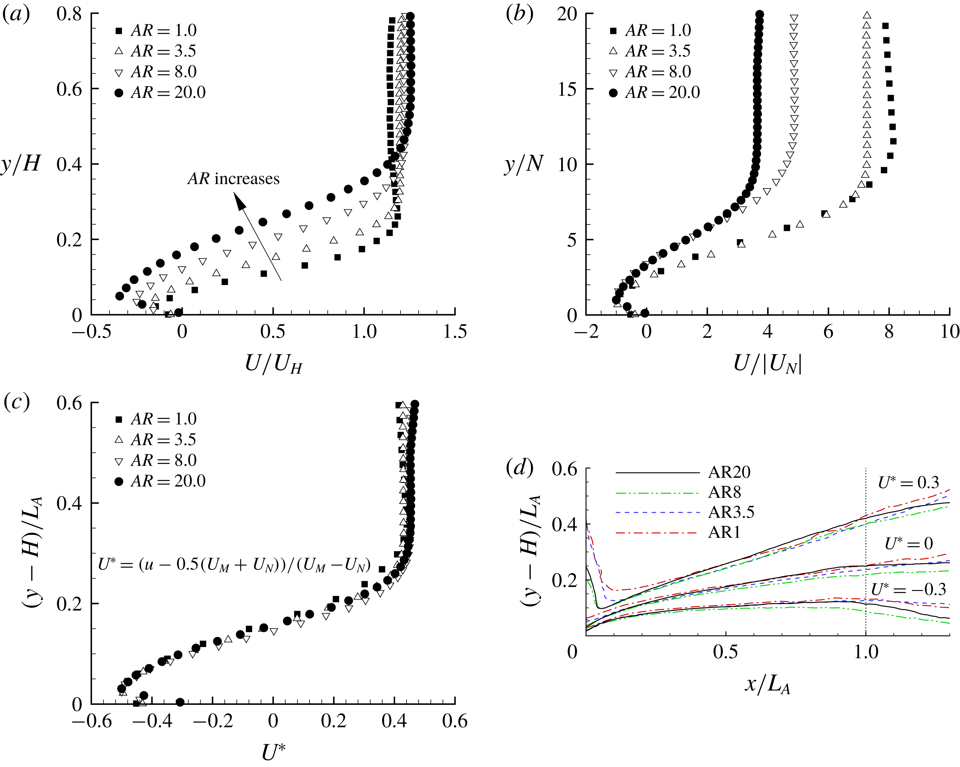
Examination of different scaling laws for the mean flow over the top surface. (a–c) These are the vertical profiles of
 $U$
at the vortex core of mean separation bubbles using different velocity and length scales. Not all measurement points are plotted for clarity. (d) Contours of
 $U^{\ast }$
using
 $L_{A}$
as the length scale.

For geometry-induced turbulent separation bubbles, different scaling laws have been proposed with the ultimate goal of collapsing the mean flow onto a universal curve. The commonly used velocity scales include
 $U_{\infty }$
,
 $U_{H}$
,
 $U_{N}$
(minimal streamwise mean velocity), while the body height, reattachment length and vertical location of
 $U_{N}$
(hereafter denoted by
 $N$
) are the routinely adopted length scales. Figure 8(a,b) examines the suitability of these scaling laws for the vertical profiles of
 $U$
at the vortex core of mean separation bubbles over the bluff bodies. In spite of the identical oncoming flow (the same
 $U_{H}$
), the size of the separation bubbles and the magnitude of reverse flow generally increase as
 $AR$
increases, and therefore using
 $U_{H}$
and
 $H$
as the velocity and length scales fails to collapse the mean velocities in different
 $AR$
cases, as shown in figure 8(a). Figure 8(b) shows that the minimum velocity (
 $U_{N}$
) and the corresponding wall-normal distance (
 $N$
) proposed by Simpson, Chew & Shivaprasad (Reference Simpson, Chew and Shivaprasad1981) and Simpson (Reference Simpson1983) is only successful in collapsing the measured data in the immediate vicinity of the wall (
 $y/N\leqslant 1$
). Simpson (Reference Simpson1989) remarked that this scaling does not work well above the location of minimum velocity. Le, Moin & Kim (Reference Le, Moin and Kim1997) and Skote & Henningson (Reference Skote and Henningson2002) showed that, for separation bubbles induced by an adverse pressure gradient and a backward-facing step (BFS), Simpson’s scales were of limited usefulness even below the location of minimum velocity.
Evidently, the mean separation bubble over the bluff bodies increases with
 $AR$
. As such, both the height (
 $H_{A}$
, measured as the maximum vertical location of the separating streamline) and reattachment length (
 $L_{A}$
) depend on
 $AR$
. However, the ratio
 $L_{A}/H_{A}$
is approximately 6.5 for all the cases, which is comparable to
 $L_{A}/H_{A}\in [6.36,6.67]$
over FFS reported by Nematollahi & Tachie (Reference Nematollahi and Tachie2018). Therefore,
 $L_{A}$
could be a promising length scale to collapse profiles in different
 $AR$
cases. For the streamwise mean velocity, we propose the following dimensionless variable:
 $$\begin{eqnarray}U^{\ast }=\frac{U-0.5(U_{M}+U_{N})}{U_{M}-U_{N}}.\end{eqnarray}$$
In (3.1),
 $U_{M}$
and
 $U_{N}$
represent the maximum and minimal streamwise mean velocities, respectively, at the streamwise location. The numerator of (3.1) represents the mean velocity viewed in a reference frame travelling in the streamwise direction at
 $0.5(U_{M}+U_{N})$
. As evident in figure 8(c),
 $L_{A}$
and
 $U^{\ast }$
successfully collapse all the vertical profiles very well. Figure 8(d) further reveals that the proposed scaling works well within the separation bubble, but deteriorates at the leading edge and downstream of the reattachment point. At the leading edge, the vertical profiles apparently scale with
 $U_{H}$
and
 $H$
(see figure 5
a), and are independent of the size of separation bubble. Downstream the separation bubble, the usefulness of
 $L_{A}$
diminishes.
3.3 Reynolds stresses
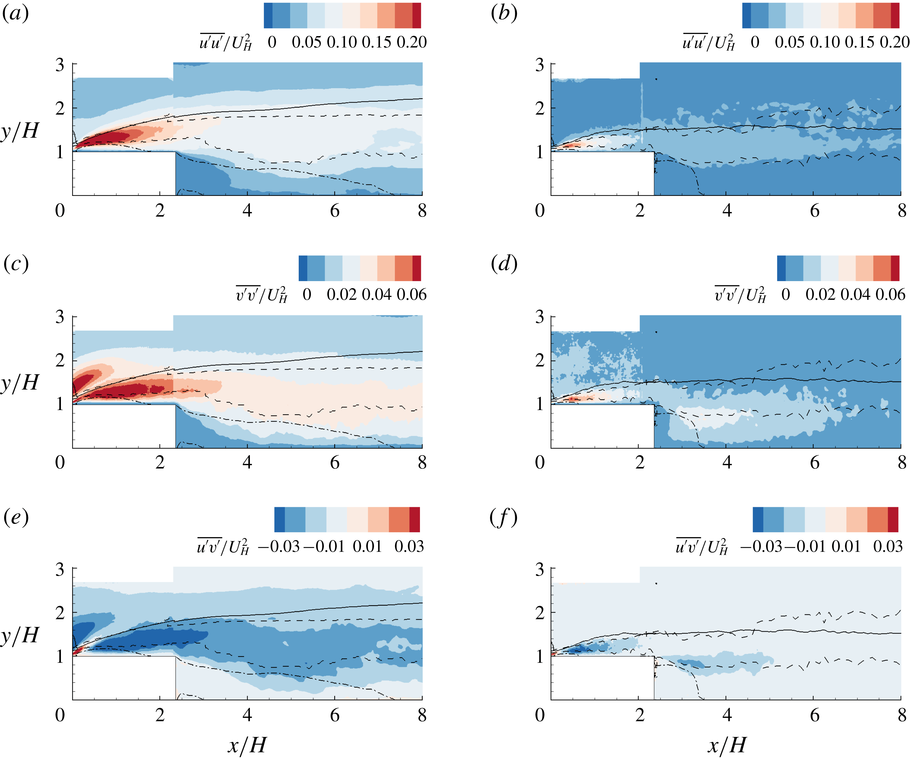
Contour of Reynolds stresses (
 $\overline{u^{\prime }u^{\prime }}$
,
 $\overline{v^{\prime }v^{\prime }}$
and
 $\overline{u^{\prime }v^{\prime }}$
) for the AR20 (a,c,e) and AR1 (b,d,f) cases. The solid and dash–dot isopleths are
 $U=U_{H}$
and
 $U=0$
, respectively. The dashed curves are the upper and lower bounds for the region of
 $u_{rms}^{\prime }\geqslant 0.8u_{rms,\max }^{\prime }$
, where
 $u_{rms,\max }^{\prime }$
denotes the maximum
 $u_{rms}^{\prime }$
at the same streamwise location. Here, the subscript
 $(\cdot )_{rms}$
denotes the root-mean-square value.

Figure 9 shows contours of the measured Reynolds stresses in the mid-span for the AR20 and AR1 cases, which are the two extreme cases examined in the present study. In general, all Reynolds stresses possess peak magnitudes near the leading edge and decay in the streamwise direction. This pattern is at variance with the distribution of Reynolds stresses over a bluff body with oncoming low turbulence levels. Specifically, with an upstream laminar flow, the shear layer in the rear part of the separation bubble becomes unstable due to Kelvin–Helmholtz instability (Alam & Sandham Reference Alam and Sandham2000; Yang & Voke Reference Yang and Voke2001; Lanzerstorfer & Kuhlmann Reference Lanzerstorfer and Kuhlmann2012), and therefore, Reynolds stresses peak around or downstream the reattachment point (Kiya & Sasaki Reference Kiya and Sasaki1983; Djilali & Gartshore Reference Djilali and Gartshore1991; Anand & Sarkar Reference Anand and Sarkar2017). The strong Reynolds stresses near the leading edge are attributed to the perturbation of upstream TBL on the shear layer emanating from the leading edge. This is consistent with the conclusion by Samson & Sarkar (Reference Samson and Sarkar2016) that higher levels of oncoming turbulence intensity can induce early turbulence transition at the separating point. It is also interesting to note that both
 $\overline{v^{\prime }v^{\prime }}$
and
 $\overline{u^{\prime }v^{\prime }}$
in the AR20 case possess two distinct regions of comparable peaks near the leading edge: one close to the isopleth of
 $U=0$
and the other above the isopleth of
 $U_{H}$
. In the AR1 case,
 $\overline{v^{\prime }v^{\prime }}$
and
 $\overline{u^{\prime }v^{\prime }}$
only peak around the isopleth of
 $U=0$
. The pattern of comparable dual peaks in
 $\overline{v^{\prime }v^{\prime }}$
and
 $\overline{u^{\prime }v^{\prime }}$
near the leading edge seems to be unique for 2-D bluff bodies with an oncoming thick TBL and high turbulence level, as in the present study. Essel & Tachie (Reference Essel and Tachie2017) and Graziani et al. (Reference Graziani, Kerhervé, Martinuzzi and Keirsbulck2018) did not observe comparable dual peaks in
 $\overline{v^{\prime }v^{\prime }}$
or
 $\overline{u^{\prime }v^{\prime }}$
for the flows over an FFS with upstream turbulence intensity of 10 % and 0.6 %, respectively. Nematollahi & Tachie (Reference Nematollahi and Tachie2018) showed that the peak magnitudes in
 $\overline{v^{\prime }v^{\prime }}$
and
 $\overline{u^{\prime }v^{\prime }}$
above the leading edge of an FFS increased as the oncoming turbulence intensity (
 $I_{u}^{\ast }$
) increased from 9.6 % to 18.7 %. Hearst et al. (Reference Hearst, Gomit and Ganapathisubramani2016) did not observe comparable dual peaks in
 $\overline{u^{\prime }v^{\prime }}$
for flows over a surface-mounted cube with oncoming TBL of
 $\unicode[STIX]{x1D6FF}\approx 2H$
and
 $I_{u}^{\ast }\in [5.4\,\%,9.0\,\%]$
.
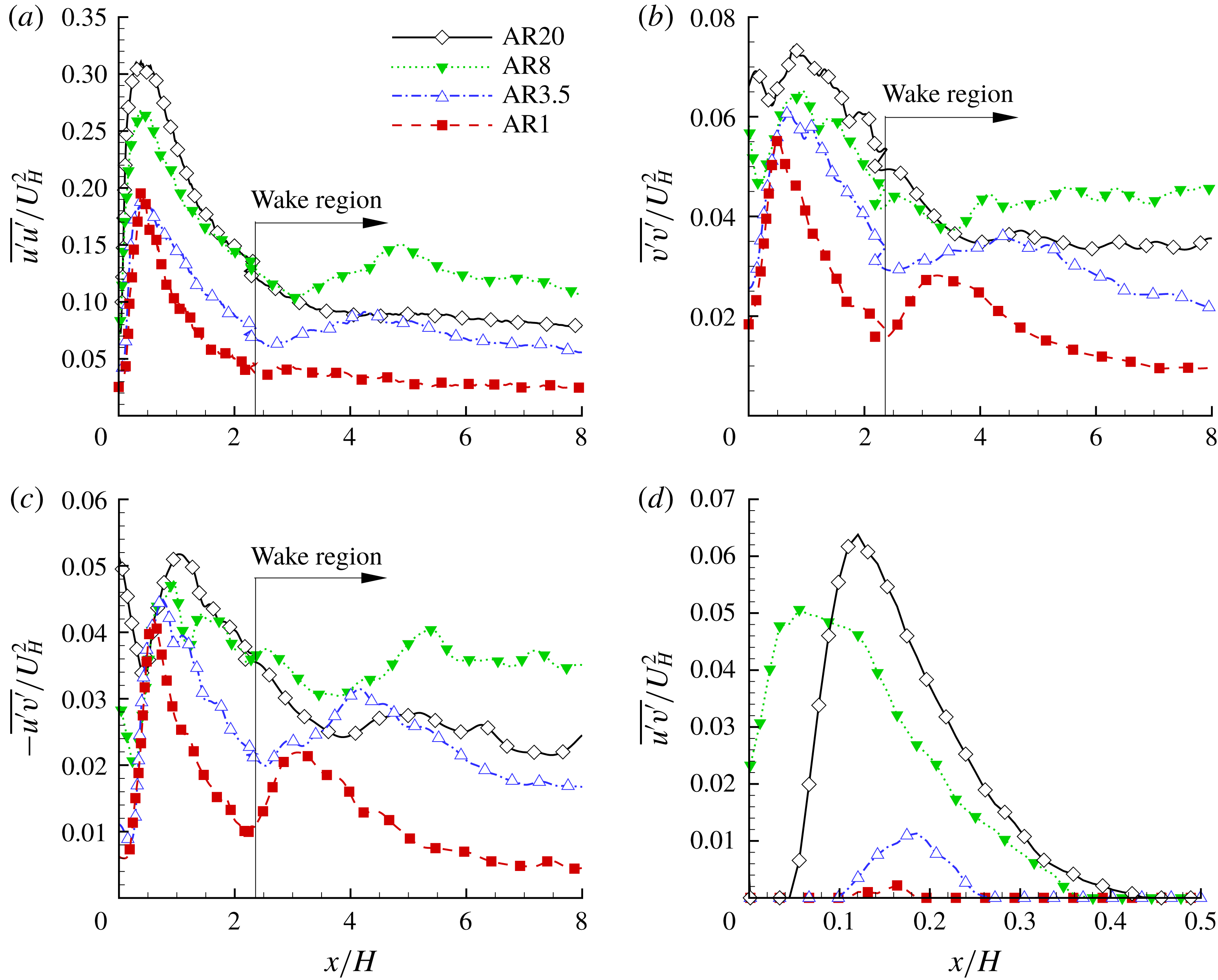
Streamwise variation of the maximum Reynolds stresses: (a)
 $\overline{u^{\prime }u^{\prime }}$
, (b)
 $\overline{v^{\prime }v^{\prime }}$
, (c)
 $-\overline{u^{\prime }v^{\prime }}$
and (d)
 $\overline{u^{\prime }v^{\prime }}$
in the vertical profiles. Note that (c,d) emphasize the maximum magnitudes of the negatively and positively valued
 $\overline{u^{\prime }v^{\prime }}$
, respectively.

To facilitate comparison of the Reynolds stresses in the different
 $AR$
cases, figure 10 plots the streamwise variation of maximum
 $\overline{u^{\prime }u^{\prime }}$
,
 $\overline{v^{\prime }v^{\prime }}$
,
 $-\overline{u^{\prime }v^{\prime }}$
and
 $\overline{u^{\prime }v^{\prime }}$
. Along the bluff bodies (
 $x/H<2.36$
), the magnitudes of Reynolds stresses generally increase as
 $AR$
increases. Dual peaks in
 $\overline{v^{\prime }v^{\prime }}$
and
 $-\overline{u^{\prime }v^{\prime }}$
are evident near the leading edge, and the peaks closer to the leading edge become trivial as
 $AR$
decreases from 20 to 3.5 and almost disappear in the AR1 case. It is also interesting to see from figure 10(a–c) that the Reynolds stresses in the wake region of the AR8 case are generally stronger than all the other cases. By comparing figures 10(c) and 10(d), it is observed that the peak magnitudes of negative
 $\overline{u^{\prime }v^{\prime }}$
and positive
 $\overline{u^{\prime }v^{\prime }}$
are comparable in the AR20 and AR8 cases, whereas the latter is significantly smaller than the former in the AR3.5 and AR1 cases. Through a coordinate transformation, Fang & Tachie (Reference Fang and Tachie2019) showed that the positive
 $\overline{u^{\prime }v^{\prime }}$
near the leading edge in the AR20 case is an artefact of misalignment between the mean streamlines and the
 $x$
coordinate defined along the bluff body (see figure 2). As seen in figures 4 and 5(a), near the leading edge, the angle between the mean streamlines and the
 $x$
direction increases as
 $AR$
increases. As such, a weaker positive
 $\overline{u^{\prime }v^{\prime }}$
occurs with a milder streamline curvature for smaller
 $AR$
.
As noted above, the present pattern of Reynolds stresses is at variance with those over bluff bodies with oncoming laminar flows or thin TBL with characteristic low turbulence level at the body height. To provide a deeper insight into the Reynolds stress field, we examine the production terms of Reynolds stresses in the mid-span. It is straightforward that
 $\unicode[STIX]{x2202}U/\unicode[STIX]{x2202}z=\unicode[STIX]{x2202}V/\unicode[STIX]{x2202}z=0$
holds in the mid-span. As such, the production terms for
 $\overline{u^{\prime }u^{\prime }}$
,
 $\overline{v^{\prime }v^{\prime }}$
and
 $\overline{u^{\prime }v^{\prime }}$
(denoted by
 $P_{uu}$
,
 $P_{vv}$
and
 $P_{uv}$
, respectively) can be simplified as follows:
 $$\begin{eqnarray}\displaystyle & \displaystyle P_{uu}=\underbrace{-2\overline{u^{\prime }u^{\prime }}\frac{\unicode[STIX]{x2202}U}{\unicode[STIX]{x2202}x}\vphantom{\frac{\unicode[STIX]{x2202}U}{\unicode[STIX]{x2202}y}}}_{P_{uu-n}}\underbrace{-2\overline{u^{\prime }v^{\prime }}\frac{\unicode[STIX]{x2202}U}{\unicode[STIX]{x2202}y}}_{P_{uu-s}}, & \displaystyle\end{eqnarray}$$
 $$\begin{eqnarray}\displaystyle & \displaystyle P_{vv}=\underbrace{-2\overline{u^{\prime }v^{\prime }}\frac{\unicode[STIX]{x2202}V}{\unicode[STIX]{x2202}x}\vphantom{\frac{\unicode[STIX]{x2202}U}{\unicode[STIX]{x2202}y}}}_{P_{vv-s}}\underbrace{-2\overline{v^{\prime }v^{\prime }}\frac{\unicode[STIX]{x2202}V}{\unicode[STIX]{x2202}y}}_{P_{vv-n}}, & \displaystyle\end{eqnarray}$$
and
 $$\begin{eqnarray}P_{uv}=\underbrace{-\overline{u^{\prime }u^{\prime }}\frac{\unicode[STIX]{x2202}V}{\unicode[STIX]{x2202}x}\vphantom{\frac{\unicode[STIX]{x2202}U}{\unicode[STIX]{x2202}y}}}_{P_{uv-nV}}\underbrace{-\overline{v^{\prime }v^{\prime }}\frac{\unicode[STIX]{x2202}U}{\unicode[STIX]{x2202}y}\vphantom{\frac{\unicode[STIX]{x2202}U}{\unicode[STIX]{x2202}y}}}_{P_{uv-nU}}\underbrace{-\overline{u^{\prime }v^{\prime }}\frac{\unicode[STIX]{x2202}U}{\unicode[STIX]{x2202}x}\vphantom{\frac{\unicode[STIX]{x2202}U}{\unicode[STIX]{x2202}y}}}_{P_{uv-sU}}\underbrace{-\overline{u^{\prime }v^{\prime }}\frac{\unicode[STIX]{x2202}V}{\unicode[STIX]{x2202}y}}_{P_{uv-sV}},\end{eqnarray}$$
respectively. In the above equations, the production terms are further decomposed into different contributions (see the notation beneath each term):
 $P_{uu-n}$
,
 $P_{vv-n}$
,
 $P_{uv-nV}$
and
 $P_{uv-nU}$
represent contributions from the Reynolds normal stresses, whereas
 $P_{uu-s}$
,
 $P_{vv-s}$
,
 $P_{uv-sU}$
and
 $P_{uv-sV}$
are contributions from the Reynolds shear stress.
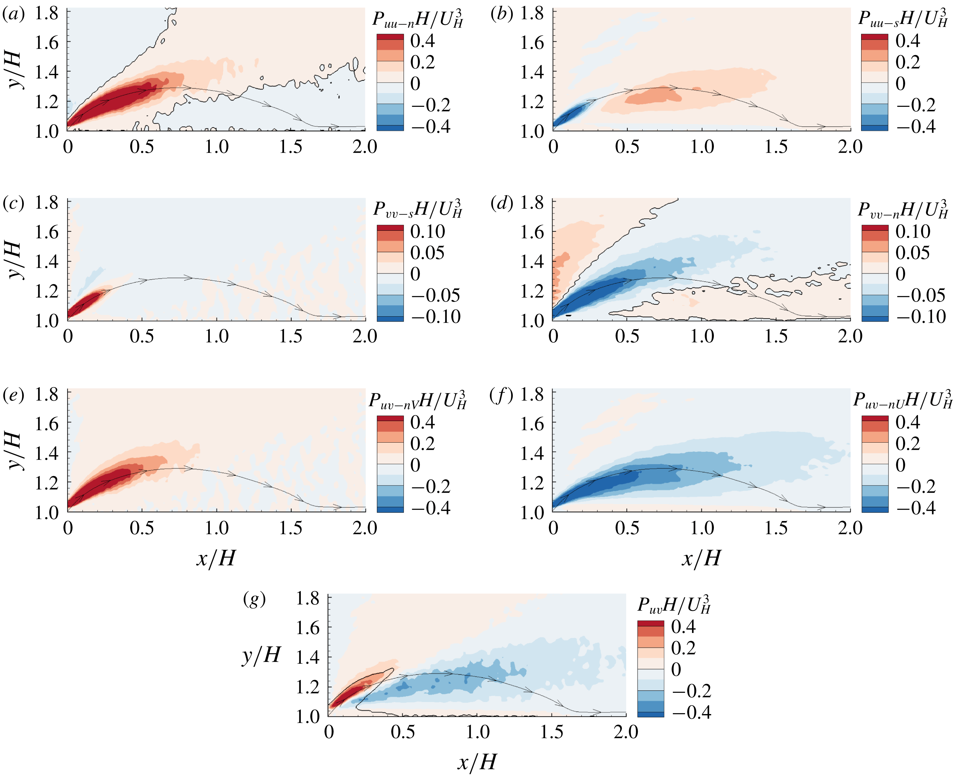
Contours of the production terms for
 $\overline{u^{\prime }u^{\prime }}$
,
 $\overline{v^{\prime }v^{\prime }}$
and
 $\overline{u^{\prime }v^{\prime }}$
over the step in the AR20 case. The separating streamline traced from the leading edge is plotted as a position reference. In (a,d), the plotted isopleths encompass positive and negative productions, respectively. In (g), the isopleth encompasses the area of positively valued
 $\overline{u^{\prime }v^{\prime }}$
.

Figure 11 shows contours of the individual production terms for the Reynolds stresses over the step in the AR20 case. Due to the nominal spanwise homogeneity in the vicinity of mid-span in the AR20 case,
 $P_{uv-sU}+P_{uv-sV}=-\overline{u^{\prime }v^{\prime }}(\unicode[STIX]{x2202}U/\unicode[STIX]{x2202}x+\unicode[STIX]{x2202}V/\unicode[STIX]{x2202}y)=\overline{u^{\prime }v^{\prime }}\unicode[STIX]{x2202}W/\unicode[STIX]{x2202}z=0$
holds, thus the net contributions from
 $P_{uv-sU}$
and
 $P_{uv-sV}$
are trivial and not plotted here. By comparing figures 11(a) and 11(b), it is interesting to see that, near the leading edge and along the separating streamline,
 $P_{uu-n}$
and
 $P_{uu-s}$
are respectively of positive and negative sign, and the former possesses larger magnitudes in a larger area than the latter. This is in sharp contrast to the zero-pressure-gradient (ZPG) TBL, where
 $P_{uu-s}$
is always the dominant positive production term (Pope Reference Pope2000). It should be noted that the positively and negatively valued
 $P_{uu-n}$
serve as self-sustaining and self-destructing mechanisms for
 $\overline{u^{\prime }u^{\prime }}$
. Specifically, as a large-scale structure (such as the near-wall streaky structure will be discussed in § 3.6) residing in the oncoming TBL passes over the step, by virtue of its interaction with the mean velocity gradient
 $\unicode[STIX]{x2202}U/\unicode[STIX]{x2202}x$
, the instantaneous Reynolds stress
 $u^{\prime }u^{\prime }$
tends to be enhanced near the narrow area emanating from the leading edge, where
 $P_{uu-n}$
is positive, but
 $u^{\prime }u^{\prime }$
is generally suppressed in the region of negatively valued
 $P_{uu-n}$
. As seen in figure 11(b), the positively valued
 $\overline{u^{\prime }v^{\prime }}$
near the leading edge generate negative production
 $P_{uu-s}$
to mitigate the self-sustaining strong
 $\overline{u^{\prime }u^{\prime }}$
.
Due to the continuity principle (
 $\unicode[STIX]{x2202}U/\unicode[STIX]{x2202}x=-\unicode[STIX]{x2202}V/\unicode[STIX]{x2202}y$
),
 $P_{vv-n}$
is always of the opposite sign of
 $P_{uu-n}$
(see figure 11
a,d). Near the leading edge along the separating streamline, the high levels of negatively valued
 $P_{vv-n}$
apparently dominate over the positively valued
 $P_{vv-s}$
. As a consequence, the net production term
 $P_{vv}$
becomes an energy sink for
 $\overline{v^{\prime }v^{\prime }}$
in that area. This is consistent with the distinct narrow area of relatively low
 $\overline{v^{\prime }v^{\prime }}$
levels appears near the leading edge of the step (see figure 9
c).
As seen in figures 11(e) and 11(f), near the leading edge of the step,
 $P_{uv-nV}$
and
 $P_{uv-nU}$
tend to generate positively valued and negatively valued
 $\overline{u^{\prime }v^{\prime }}$
, respectively. These two opposite production terms switch dominance along the separating streamline, with the positive production prevailing immediately upstream of the separation bubble (see figure 11
g). Although not shown here, contours of the production terms in other cases exhibit patterns similar to those in the AR20 case, except that in general, the magnitudes of all production terms decrease as
 $AR$
decreases.
3.4 Streamwise–spanwise vortex shedding in the wake region
It is generally acknowledged that the vortical structures behind bluff bodies are sensitive to their slenderness defined as the height-to-width ratio
 $H/S$
, or equivalently,
 $1/\mathit{AR}$
. Sakamoto & Arie (Reference Sakamoto and Arie1983) measured the vortex shedding motions behind surface-mounted rectangular prisms with different slenderness (
 $H/S=H/L\in [1,8]$
), and observed two distinct types of vortex shedding: antisymmetric Kármán-type vortices prevailing for
 $H/S>2$
, and symmetric arch-type vortices prevailing for
 $H/S<2$
. Wang et al. (Reference Wang, Zhou, Chan and Lam2006) experimentally investigated the effect of different oncoming TBLs (
 $\unicode[STIX]{x1D6FF}/H\in [0.1,0.38]$
) on the wake flow behind a square cylinder with
 $H/S=5$
using both a laser Doppler anemometer (LDA) and PIV. They observed that with a thicker TBL, the probability of antisymmetric vortices decreases near the wall but increases near the free end. Meanwhile, Wang & Zhou (Reference Wang and Zhou2009) studied the wake flow behind square cylinders (
 $H/S\in [3,11]$
) immersed in a thin TBL (
 $\unicode[STIX]{x1D6FF}/H\in [0.12,0.45]$
) using hot-wire, PIV and laser-induced fluorescence techniques. They observed that the antisymmetric vortex shedding occurred intermittently depending on the appearance of wall-normal flow motions. It should be noted that all the aforementioned studies focused on the wake flows behind either a square or circular cylinder with oncoming thin TBLs (
 $\unicode[STIX]{x1D6FF}/H<1$
). To the best knowledge of the authors, the interaction of a thick TBL (
 $\unicode[STIX]{x1D6FF}/H>1$
) with bluff bodies with different spanwise widths in terms of vortex shedding in the wake flow in the streamwise–spanwise plane has not been studied.
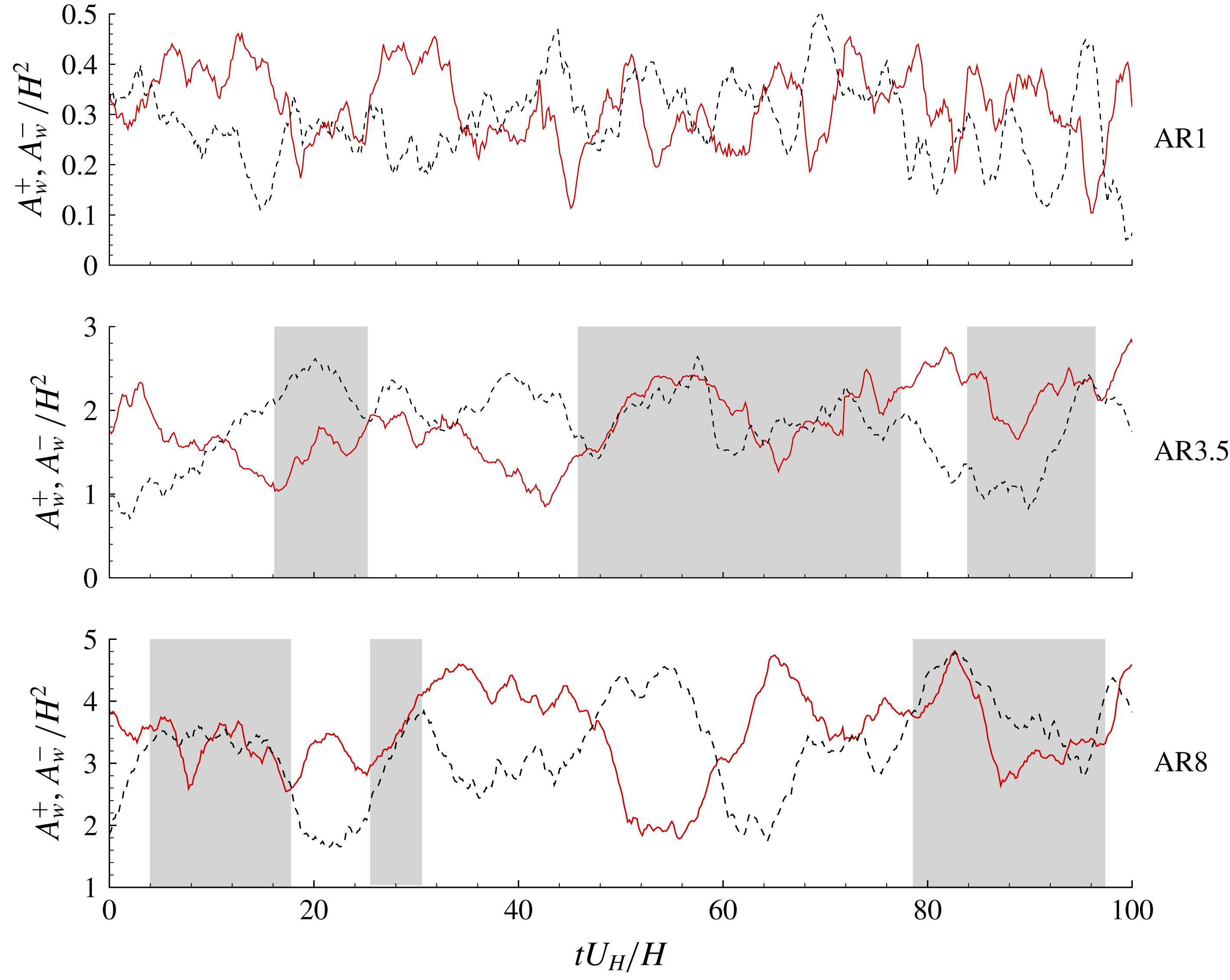
Time sequences of the areas of reverse flow in regions of
 $z/H\in [0,1]$
(
 $A_{w}^{+}$
, solid lines) and
 $z/H\in [-1,0]$
(
 $A_{w}^{-}$
, dotted lines) for different cases. The shaded areas highlight intervals of synchronized variation of
 $A_{w}^{+}$
and
 $A_{w}^{-}$
.

In the present 3-D cases, the mean reverse flow is concentrated near the mid-span and is associated with two large-scale counter-rotating vortices in the
 $x$
–
 $z$
plane behind the bluff bodies (see figure 6
b). This is consistent with the well-known arch-shaped vortex behind the 3-D bluff bodies (Martinuzzi & Tropea Reference Martinuzzi and Tropea1993; Hussein & Martinuzzi Reference Hussein and Martinuzzi1996). The arch-shaped vortex is likely influenced by vortex shedding from the side walls of the bluff bodies and, therefore, is unsteady in time. In view of the intimate connection between arch-shaped vortex with reverse flows in the wake, figure 12 compares the time sequences of reverse flow areas in the regions
 $z/H\in [0,1]$
(denoted by
 $A_{w}^{+}$
, which is calculated by summing the area of negative
 $u$
for
 $z/H\in [0,1]$
) and
 $z/H\in [-1,0]$
(denoted by
 $A_{w}^{-}$
, which is calculated by summing the area of negative
 $u$
for
 $z/H\in [-1,0]$
) at
 $y/H=0.5$
for both 3-D bluff bodies (AR1 and AR3.5) and a transitional configuration (AR8). As seen in the figure, the temporal variation of
 $A_{w}^{+}$
and
 $A_{w}^{-}$
alternates between antisymmetric and synchronized patterns in the AR3.5 and AR8 cases, whereas
 $A_{w}^{+}$
and
 $A_{w}^{-}$
in the AR1 case show a persistent antisymmetric temporal variation. The synchronized variation of
 $A_{w}^{+}$
and
 $A_{w}^{-}$
can be induced by either a symmetric vortex shedding from the two side walls or the flapping motion in the
 $x$
–
 $y$
plane of TSBB near the mid-span. The distinction of these two mechanisms are beyond the scope of this paper. Nonetheless, the antisymmetric temporal variation of
 $A_{w}^{+}$
and
 $A_{w}^{-}$
reflects the antisymmetric vortex shedding from two side walls.
The spatial characteristics of the vortex shedding in the wake region are examined using the following
 $\unicode[STIX]{x1D6E4}$
function proposed by Graftieaux, Michard & Grosjean (Reference Graftieaux, Michard and Grosjean2001):
 $$\begin{eqnarray}\unicode[STIX]{x1D6E4}=\frac{1}{M}\mathop{\sum }_{P\in {\mathcal{A}}}\frac{(\unicode[STIX]{x1D616}\unicode[STIX]{x1D617}\times \unicode[STIX]{x1D61C}_{\unicode[STIX]{x1D617}})\boldsymbol{\cdot }\boldsymbol{y}}{\Vert \unicode[STIX]{x1D616}\unicode[STIX]{x1D617}\Vert \boldsymbol{\cdot }\Vert \unicode[STIX]{x1D61C}_{\unicode[STIX]{x1D617}}\Vert }.\end{eqnarray}$$
In the above equation,
 $M$
denotes the number of points (
 $\unicode[STIX]{x1D617}$
) in the square area of
 ${\mathcal{A}}$
centred at point
 $\unicode[STIX]{x1D616}$
. As such, the summed fraction quantifies the sine of the angle between radius vector
 $\unicode[STIX]{x1D616}\unicode[STIX]{x1D617}$
and velocity vector
 $\unicode[STIX]{x1D61C}_{\unicode[STIX]{x1D617}}$
. Therefore, a larger positive (negative)
 $\unicode[STIX]{x1D6E4}$
indicates well-organized counter-clockwise (clockwise) swirling motion surrounding the point
 $\unicode[STIX]{x1D616}$
. The side length of
 ${\mathcal{A}}$
is chosen as
 $0.8H$
, a value that is close to the streamwise distance of mean vortical core from the leeward face of the bluff bodies.
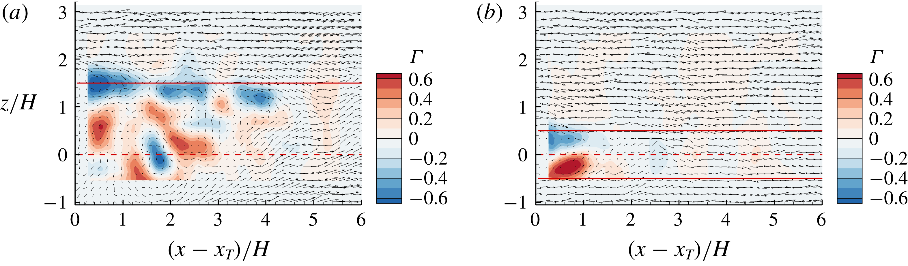
Instantaneous velocity vectors superimposed with contours of
 $\unicode[STIX]{x1D6E4}$
in the (a) AR3.5 and (b) AR1 cases. Horizontal lines mark the spanwise locations of the side walls, and dashed lines mark the mid-span. Here
 $x_{T}$
denotes the streamwise location of the trailing edge, i.e.
 $x_{T}/H=2.36$
.

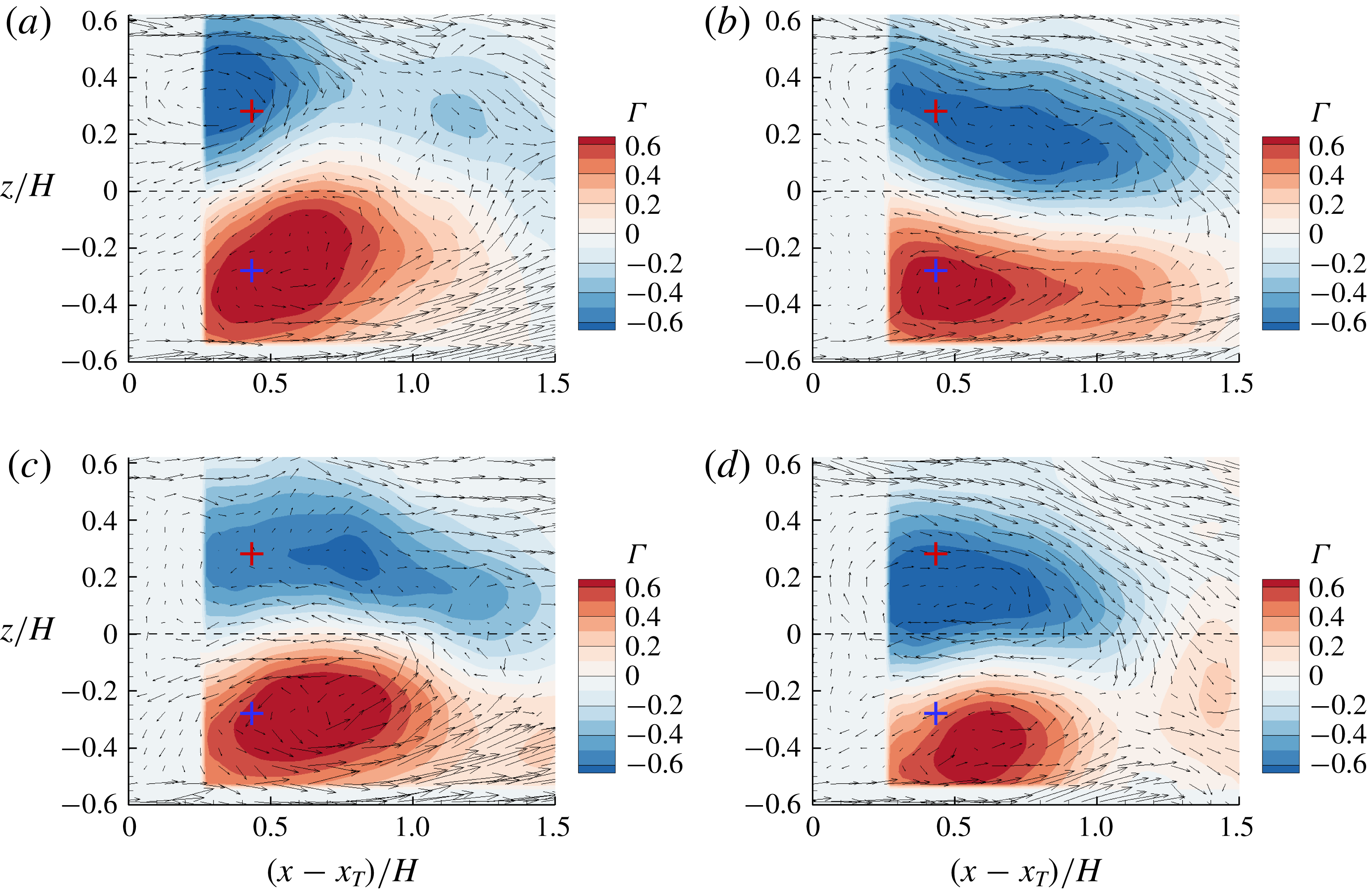
Consecutive snapshots of instantaneous velocity vectors and contours of
 $\unicode[STIX]{x1D6E4}$
in the AR1 case. The time interval between adjacent figures is
 $3.6H/U_{H}$
. The crosses mark the vortex cores of the mean swirling motion.

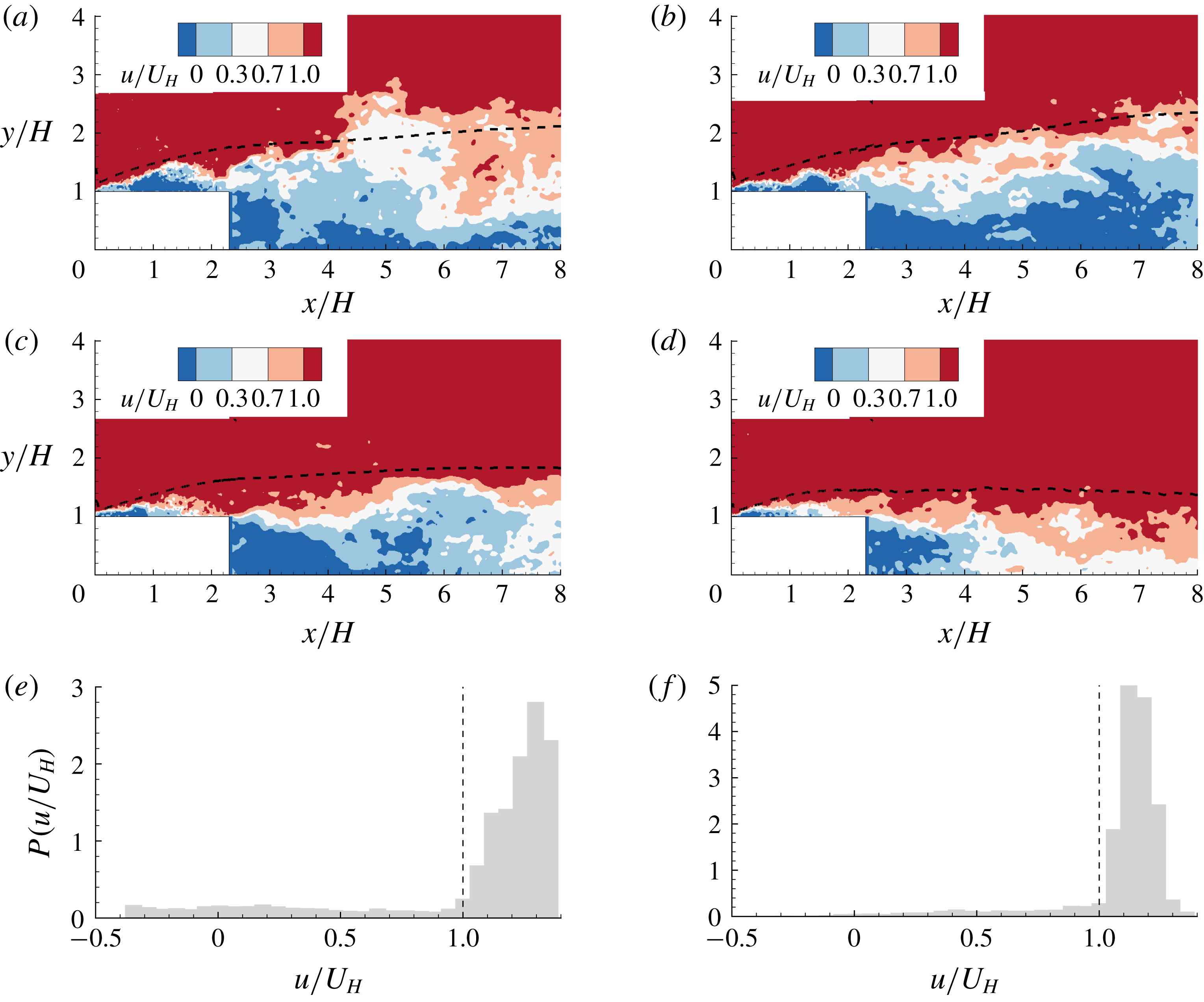
Figure 13 shows typical instantaneous velocity fields in the AR3.5 and AR1 cases. In the AR3.5 case, multiple anti-clockwise vortices appear directly behind the side wall, and both anti-clockwise and clockwise vortices occur near the mid-span. In contrast, as seen in figure 13(b), a pair of counter-rotating vortices appear behind the bluff body in the AR1 case. These observations indicate that for a large
 $AR$
(say
 $AR\geqslant 3.5$
), the spanwise width of the bluff body is significantly larger than the diameters of the vortices, and therefore the vortex shedding motions from the two side walls hardly interact with each other and tend to behave independently. Figure 14 shows contours of
 $\unicode[STIX]{x1D6E4}$
at consecutive time snapshots in the AR1 case. In general, the size and strength of the vortices on both sides of the mid-span alternate in time. Based on figures 13(b) and 14, the arch-shaped vortex in the AR1 case is persistent in time, but its two legs alternate in size and strength.
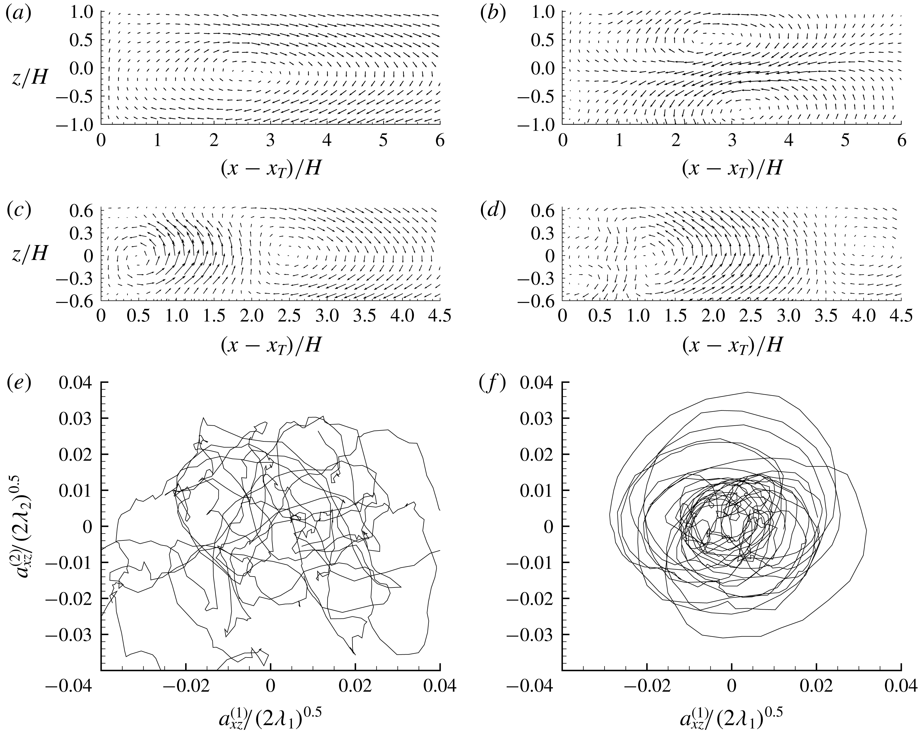
(a,b) The first and second POD modes in the AR3.5 case. (c,d) The first and second POD modes in the AR1 case. (e,f) The temporal trajectories of the coefficients of the first two POD modes (
 $a_{xz}^{(1)}$
and
 $a_{xz}^{(2)}$
) in the AR3.5 and AR1 cases, respectively.

Proper orthogonal decomposition (POD) is further used to examine coherent structures in the
 $x$
–
 $z$
plane in the AR3.5 and AR1 cases. As seen in figure 15(a,b,e) for the AR3.5 case, the first and second POD modes are antisymmetric and symmetric, respectively, about the mid-span (
 $z/H=0$
), and their coefficients (
 $a_{xz}^{(1)}$
and
 $a_{xz}^{(2)}$
) are most likely uncorrelated. In view of this, the pattern of alternating antisymmetric and symmetric variations of
 $A_{w}^{+}$
and
 $A_{w}^{-}$
observed in figure 12 can be attributed to the switching of dominance between the first and second POD modes. In contrast, in the AR1 case (figure 15
c,d,f), the first two POD modes clearly exhibit an anti-symmetric pattern, and their coefficients form circular phase portrait (see figure 15
f). This is consistent with the persistent antisymmetric variations of
 $A_{w}^{+}$
and
 $A_{w}^{-}$
shown in figure 12 for the AR1 case. The circular phase portrait of the first two POD modes in figure 15(f) is similar to that for the wake flow behind a circular or square cylinder, commonly recognized as the footprint of energetic vortex shedding (Deane et al.
Reference Deane, Kevrekidis, Karniadakis and Orszag1991; Ma & Karniadakis Reference Ma and Karniadakis2002; Wee et al.
Reference Wee, Yi, Annaswamy and Ghoniem2004; van Oudheusden et al.
Reference van Oudheusden, Scarano, van Hinsberg and Watt2005).
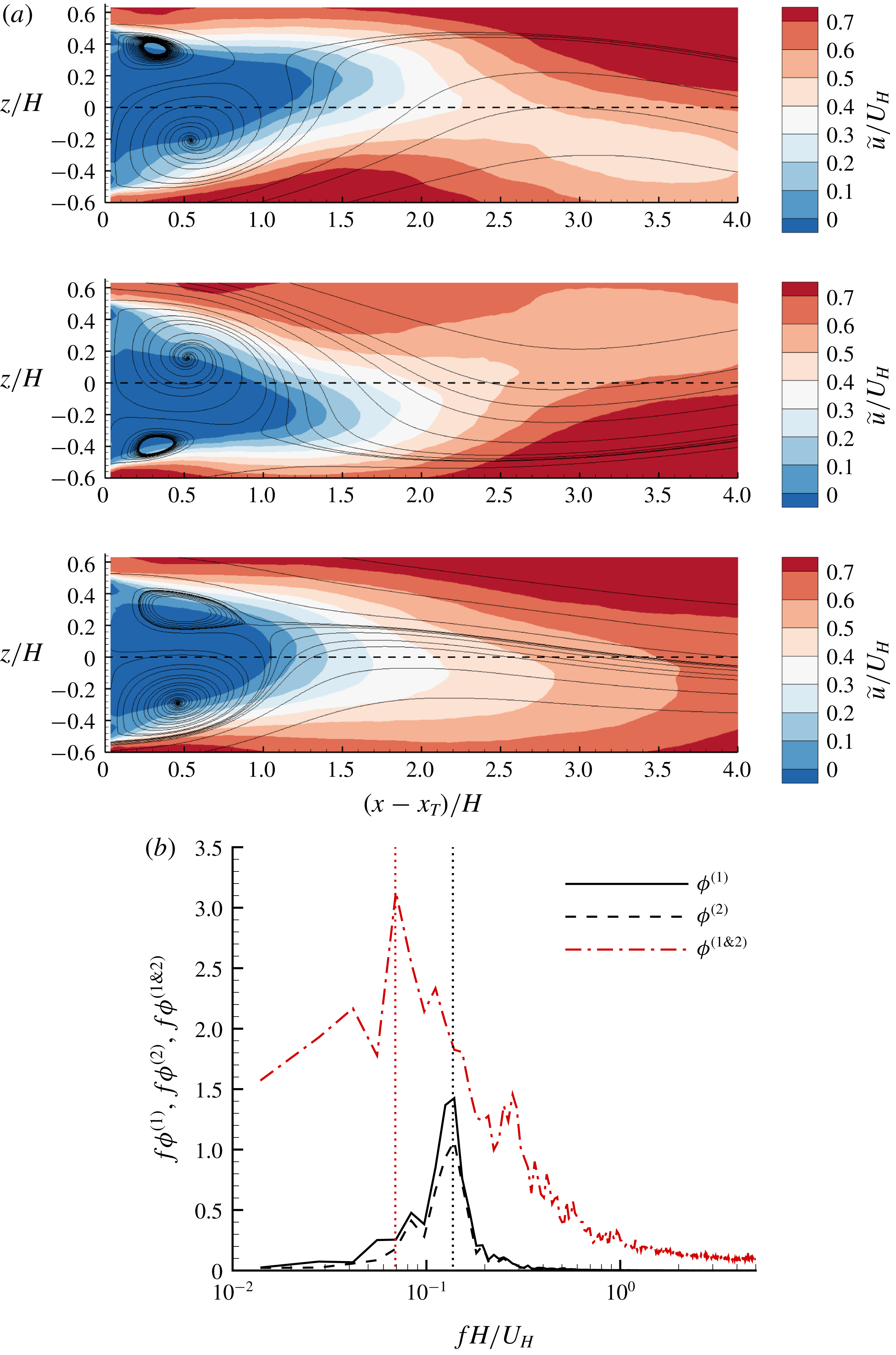
(a) Streamlines of the low-order representation using the first two POD modes in the AR1 cases. The time interval between two adjacent figures is
 $5H/U_{H}$
. An animation is also shown in a supplementary video available at https://doi.org/10.1017/jfm.2019.617. (b) Premultiplied frequency spectra of the coefficients of the first two POD modes (
 $\unicode[STIX]{x1D719}^{(1)}$
and
 $\unicode[STIX]{x1D719}^{(2)}$
) as well as the radius of orbits in figure 15(f) (
 $\unicode[STIX]{x1D719}^{(1\& 2)}$
) in the AR1 case. The two vertical dotted lines are at
 $St=0.07$
and 0.14, respectively.

Figure 16(a) shows consecutive snapshots of streamlines reconstructed using the mean flow and the first two POD modes. It is evident that the recirculation bubbles alternate in size, shifting the reverse flow area (see the dashed curves) from left to right. Thus the flow topology shown in figure 16(a) is the superposition of the mean flow with antisymmetric vortex shedding from the two side walls. As seen in figure 16(b), the dominant frequency of the vortex shedding motion, indicated by the first two POD modes, is at
 $St=0.14$
.
In the case of a laminar flow with a perfect periodic vortex shedding, the temporal trajectory of the coefficients of first two POD modes forms a perfect circular orbit (Noack et al.
Reference Noack, Afanasiev, Morzyński, Tadmor and Thiele2003). As such, the phase angle, defined as
 $\unicode[STIX]{x1D703}=\tan ^{-1}[(a_{xz}^{(2)}\sqrt{\unicode[STIX]{x1D706}_{1,xz}})/(a_{xz}^{(1)}\sqrt{\unicode[STIX]{x1D706}_{2,xz}})]$
, is the sole variable for distinguishing different stages of vortex shedding (van Oudheusden et al.
Reference van Oudheusden, Scarano, van Hinsberg and Watt2005; Perrin et al.
Reference Perrin, Braza, Cid, Cazin, Barthet, Sevrain, Mockett and Thiele2007; Riches, Martinuzzi & Morton Reference Riches, Martinuzzi and Morton2018). However, as seen in figure 15(f), the radius of the orbits, defined as
 $r=\sqrt{[a_{xz}^{(1)}]^{2}/(2\unicode[STIX]{x1D706}_{1})+[a_{xz}^{(2)}]^{2}/(2\unicode[STIX]{x1D706}_{2})}$
, varies in time. The value of
 $r$
quantifies the amplitude/strength of the vortex shedding. The premultiplied frequency of
 $r$
(
 $\unicode[STIX]{x1D719}^{(1\& 2)}$
) shown in figure 16(b) possesses a sharp peak at
 $St=0.07$
, which coincides with the dominant frequency of the oncoming TBL (see figure 3
d). Based on the above analysis, the anti-symmetric streamwise–spanwise vortex shedding occurs in the wake region of the AR1 case at
 $St=0.14$
, and the corresponding amplitude is modulated by the oncoming TBL at
 $St=0.07$
. The observed frequency (
 $St=0.14$
) of vortex shedding is comparable to 0.13 and 0.145 reported by Hussein & Martinuzzi (Reference Hussein and Martinuzzi1996) and Hearst et al. (Reference Hearst, Gomit and Ganapathisubramani2016), respectively, for the wake flows of a surface-mounted cube. It should be noted that the oncoming flow conditions in Hussein & Martinuzzi (Reference Hussein and Martinuzzi1996) and Hearst et al. (Reference Hearst, Gomit and Ganapathisubramani2016) are drastically different (see table 1). It appears that the frequency of vortex shedding in the wake flow of the AR1 case is insensitive to the oncoming TBL. This is consistent with the observation by Vinuesa et al. (Reference Vinuesa, Schlatter, Malm, Mavriplis and Henningson2015) that the frequency of vortex shedding behind a square cylinder (
 $H/S=4$
) was the same with either a laminar or turbulent oncoming flow.
3.5 Characteristics of shear layer
Contours of instantaneous streamwise velocity (
 $u$
) in the (a) AR20, (b) AR8, (c) AR3.5 and (d) AR1 cases, respectively. In (a–d), the superimposed dashed isopleth is at
 $U=U_{H}$
. (e,f) Show the probability density function of
 $u/U_{H}$
for the instantaneous streamwise velocity over the step in (a,d), respectively.

Figure 17 shows representative instantaneous streamwise velocity fields in selected test cases. As seen in the figures, a common feature amongst the different cases is a strong shear layer emanating from the leading edge of the bluff body. In particular, this shear layer is bounded by the isopleth of
 $u=U_{H}$
in the upper portion over the bluff bodies. A statistical evidence for this observation is provided in figure 17(e,f), which presents the probability density function (PDF) of
 $u/U_{H}$
for the instantaneous streamwise velocity over the bluff body for the AR20 and AR1 cases, respectively. The counterpart plots for the AR8 and AR3.5 cases exhibit similar patterns. This analysis is inspired by the similar approach commonly used to identify instantaneous edges of uniform momentum zones (UMZ) in TBL (Adrian et al.
Reference Adrian, Meinhart and Tomkins2000; De Silva et al.
Reference De Silva, Philip, Hutchins and Marusic2017; Laskari et al.
Reference Laskari, de Kat, Hearst and Ganapathisubramani2018). It is generally acknowledged that most of the shear in TBL is concentrated across a few interfaces featuring a local minimal PDF of
 $u$
, which also varies in time (Laskari et al.
Reference Laskari, de Kat, Hearst and Ganapathisubramani2018). From figure 17(e,f), the PDF of
 $u<U_{H}$
exhibits a distinct plateau at a very low value, and there exists a sharp increase at
 $u=U_{H}$
(see the dashed vertical lines). These observations indicate that the shear layer over the bluff body is concentrated in areas where the instantaneous streamwise velocity
 $u<U_{H}$
. In the following, the isopleths of
 $u=U_{H}$
and
 $U=U_{H}$
are denoted by
 $U_{H}^{i}$
and
 $U_{H}^{I}$
, respectively, for conciseness.
Conditionally averaged (a)
 $\langle u\rangle$
, (b)
 $\langle v\rangle$
and (c)
 $\text{d}\langle u\rangle /\text{d}y$
around the isopleth of
 $u=U_{H}$
at
 $x/H=0.5$
in different cases. (d) Vertical profiles of
 $\unicode[STIX]{x2202}U/\unicode[STIX]{x2202}y$
at
 $x/H=0.5$
in different cases. In (d), thick horizontal line segments mark the locations of
 $U=U_{H}$
in different cases. Other than the inset in (c), every third measurement point is plotted for clarity.

To further understand the dynamics of the shear layer below
 $U_{H}^{i}$
deduced from figure 17, conditionally averaged statistics in the vertical neighbourhood of
 $U_{H}^{i}$
at
 $x/H=0.5$
are calculated and the results are presented in figure 18(a–c). Specifically, the lowest grid point passing
 $U_{H}^{i}$
at
 $x/H=0.5$
is fixed at
 $\langle y\rangle =0$
and the surrounding statistics are calculated. As seen in figure 18(a,c), most of the shear occurs below
 $U_{H}^{i}$
, consistent with the previous analysis for figure 17. Figure 18(c,d) shows that the peak value of
 $\text{d}\langle u\rangle /\text{d}y$
tends to occur right at
 $U_{H}^{i}$
, and is almost twice the value of
 $(\unicode[STIX]{x2202}U/\unicode[STIX]{x2202}y)_{max}$
. One important implication of this observation is that the instantaneous shear layer can be much stronger than the time-averaged value, which is commonly observed for an internal shear layer within a TBL (De Silva et al.
Reference De Silva, Philip, Hutchins and Marusic2017; Laskari et al.
Reference Laskari, de Kat, Hearst and Ganapathisubramani2018). Furthermore, as seen in figure 18(d),
 $(\unicode[STIX]{x2202}U/\unicode[STIX]{x2202}y)_{max}$
always occurs below
 $U_{H}^{I}$
. This reflects the meandering nature of
 $U_{H}^{i}$
and also indicates that the instantaneous
 $\unicode[STIX]{x2202}u/\unicode[STIX]{x2202}y$
at
 $U_{H}^{i}$
is most likely larger than
 $(\text{d}\langle u\rangle /\text{d}y)_{max}$
as
 $U_{H}^{i}$
meanders closer to the top surface. This deduction is explained as follows: the convolution of the PDF of the elevation of
 $U_{H}^{i}$
and the profile of
 $\langle u\rangle$
shown in figure 18(a) gives the profile of
 $U$
in the vicinity of
 $U_{H}$
(De Silva et al.
Reference De Silva, Philip, Hutchins and Marusic2017). By the same logic, if the instantaneous
 $\unicode[STIX]{x2202}u/\unicode[STIX]{x2202}y$
at
 $U_{H}^{i}$
was always a constant at
 $(\text{d}\langle u\rangle /\text{d}y)_{max}$
,
 $(\unicode[STIX]{x2202}U/\unicode[STIX]{x2202}y)_{max}$
would coincide with
 $U_{H}^{I}$
, which is clearly not the case. At instances when
 $U_{H}^{i}$
is very close to the top surface, the shear layer below
 $U_{H}^{i}$
is thinner and therefore larger
 $\unicode[STIX]{x2202}u/\unicode[STIX]{x2202}y$
occurs. As such,
 $(\unicode[STIX]{x2202}U/\unicode[STIX]{x2202}y)_{max}$
always occurs below
 $U_{H}^{I}$
.
The instantaneous shear layer emanating from the leading edge exhibits remarkably different characteristics from the internal shear layer in TBL. As seen in figure 18(b), the conditionally averaged
 $\langle v\rangle$
generally increases in the vertical direction. This is in contrast to the internal shear layer within a TBL (De Silva et al.
Reference De Silva, Philip, Hutchins and Marusic2017), where the instantaneous shear layer is typically flanked by large and small values of
 $\langle v\rangle$
in the upper and lower portions, respectively. This is consistent with a variable-interval time averaging (VITA) event, which features a sudden switching between ejection and sweep events, occurring along the stagnation line below the hairpin head (Blackwelder & Kaplan Reference Blackwelder and Kaplan1976; Adrian et al.
Reference Adrian, Meinhart and Tomkins2000; De Silva et al.
Reference De Silva, Philip, Hutchins and Marusic2017).
Streamwise variation of vorticity thicknesses based on (a) conditionally averaged shear layer along
 $U_{H}^{i}$
(
 $\unicode[STIX]{x1D6FF}_{\unicode[STIX]{x1D714}}^{\prime }$
) and (b) mean shear layer (
 $\unicode[STIX]{x1D6FF}_{\unicode[STIX]{x1D714}}$
) in different cases. Note in (b) that
 $\unicode[STIX]{x1D6FF}_{\unicode[STIX]{x1D714}}$
is only plotted before reattachment point, where
 $(\unicode[STIX]{x2202}U/\unicode[STIX]{x2202}y)_{max}$
is always associated with the shear layer emanating from the leading edge.

We further investigate the shear layer emanating from the leading edge using the following vorticity thicknesses:
 $\!\unicode[STIX]{x1D6FF}_{\unicode[STIX]{x1D714}}^{\prime }\,=\,U_{H}/(\text{d}\langle u\rangle /\text{d}y)_{max}$
and
 $\!\unicode[STIX]{x1D6FF}_{\unicode[STIX]{x1D714}}\,=\,(U_{max}-U_{N})/(\unicode[STIX]{x2202}U/\unicode[STIX]{x2202}y)_{max}$
, where
 $U_{max}$
(
 $\equiv U_{\infty }$
) and
 $U_{N}$
are respectively the maximum and minimum mean streamwise velocities;
 $\unicode[STIX]{x1D6FF}_{\unicode[STIX]{x1D714}}^{\prime }$
and
 $\unicode[STIX]{x1D6FF}_{\unicode[STIX]{x1D714}}$
quantify the vorticity thicknesses of conditional averaged shear layer along
 $U_{H}^{i}$
and mean shear layers, respectively. The streamwise variation of
 $\unicode[STIX]{x1D6FF}_{\unicode[STIX]{x1D714}}^{\prime }$
and
 $\unicode[STIX]{x1D6FF}_{\unicode[STIX]{x1D714}}$
for different
 $AR$
s are shown in figure 19. From figure 19(a), the vorticity thickness is drastically reduced immediately downstream of the leading edge in all the cases. The growth rate of
 $\unicode[STIX]{x1D6FF}_{\unicode[STIX]{x1D714}}^{\prime }$
,
 $\text{d}\unicode[STIX]{x1D6FF}_{\unicode[STIX]{x1D714}}^{\prime }/\text{d}x$
, evidently decreases as
 $AR$
increases. This indicates that the amplitude of the vertical meandering of the shear layer increases as
 $AR$
increases. In contrast, the linear variation of
 $\unicode[STIX]{x1D6FF}_{\unicode[STIX]{x1D714}}$
is independent of
 $AR$
with a slope of
 $\text{d}\unicode[STIX]{x1D6FF}_{\unicode[STIX]{x1D714}}/\text{d}x\approx 0.32$
. This slope is apparently larger than the commonly reported range of
 $\text{d}\unicode[STIX]{x1D6FF}_{\unicode[STIX]{x1D714}}/\text{d}x\in [0.15,0.22]$
for mixing layer (Brown & Roshko Reference Brown and Roshko1974) and separation bubbles (Kiya, Sasaki & Arie Reference Kiya, Sasaki and Arie1982; Cherry, Hillier & Latour Reference Cherry, Hillier and Latour1984; Djilali & Gartshore Reference Djilali and Gartshore1991; Lander et al.
Reference Lander, Letchford, Amitay and Kopp2016; Mohammed-Taifour & Weiss Reference Mohammed-Taifour and Weiss2016). However, it agrees very well with
 $\text{d}\unicode[STIX]{x1D6FF}_{\unicode[STIX]{x1D714}}/\text{d}x=0.33$
reported by Agelinchaab & Tachie (Reference Agelinchaab and Tachie2008) for an FFS submerged in a deep TBL (
 $\unicode[STIX]{x1D6FF}/H=9.1$
). Most recently, Nematollahi & Tachie (Reference Nematollahi and Tachie2018) observed that for an FFS, by increasing the oncoming turbulence intensity
 $I_{u}^{\ast }$
from 9.6 % to 18.7 % using different wall roughnesses,
 $\text{d}\unicode[STIX]{x1D6FF}_{\unicode[STIX]{x1D714}}/\text{d}x$
increased from 0.224 to 0.336. Thus, the enhanced growth rate of vorticity thickness
 $\text{d}\unicode[STIX]{x1D6FF}_{\unicode[STIX]{x1D714}}/\text{d}x=0.32$
compared to the more commonly reported values of
 $\text{d}\unicode[STIX]{x1D6FF}_{\unicode[STIX]{x1D714}}/\text{d}x\in [0.15,0.22]$
can be attributed to the high levels of turbulence intensity induced by the upstream deep TBL. As seen in figure 18(a), the slopes,
 $\text{d}\unicode[STIX]{x1D6FF}_{\unicode[STIX]{x1D714}}^{\prime }/\text{d}x$
, are apparently much smaller than
 $\text{d}\unicode[STIX]{x1D6FF}_{\unicode[STIX]{x1D714}}/\text{d}x$
, indicating the persistence of shear layer along
 $U_{H}^{i}$
over the bluff body. Furthermore, the shear layer emanating from the leading edge of a smaller
 $AR$
case meanders less in the vertical direction and the strength decays faster downstream of the leading edge.
Vectors of (
 $R_{vu},R_{vv}$
) superimposed with contours of
 $R_{vv}$
in the (a) AR20, (b) AR8, (c) AR3.5 and (d) AR1 cases, respectively, with the reference point at
 $(x/H,y/H)=(1.0,1.3)$
. Vectors of (
 $R_{vu},R_{vv}$
) superimposed with contours of
 $R_{vv}$
in the (e) AR20 and (f) AR1 cases, respectively, with the reference point at
 $(x/H,y/H)=(0.5,1.1)$
. All vectors are scaled to possess a unit length. The cross symbol (
 $+$
) marks the reference point. The solid, dash–dotted and dotted isopleths are 80 % of maximum
 $R_{vu}$
,
 $U=U_{H}$
and
 $U=0$
, respectively. The dashed lines mark the vertical locations of the maximum
 $\unicode[STIX]{x2202}U/\unicode[STIX]{x2202}y$
away from the top surface.

The spatial structures associated with the shear layer emanating from the leading edge are further examined using the two-point correlation function, which is defined as follows:
 $$\begin{eqnarray}R_{\unicode[STIX]{x1D701}\unicode[STIX]{x1D709}}=\frac{\overline{\unicode[STIX]{x1D701}(\boldsymbol{X}_{ref})\unicode[STIX]{x1D709}(\boldsymbol{X}_{ref}+\unicode[STIX]{x0394}\boldsymbol{X})}}{\unicode[STIX]{x1D701}_{rms}(\boldsymbol{X}_{ref})\unicode[STIX]{x1D709}_{rms}(\boldsymbol{X}_{ref}+\unicode[STIX]{x0394}\boldsymbol{X})}.\end{eqnarray}$$
Here,
 $\unicode[STIX]{x1D701}$
and
 $\unicode[STIX]{x1D709}$
denote two generalized fluctuating components (such as
 $u^{\prime }$
and
 $v^{\prime }$
) with the root-mean-square values of
 $\unicode[STIX]{x1D701}_{rms}$
and
 $\unicode[STIX]{x1D709}_{rms}$
, respectively. In (3.6),
 $\boldsymbol{X}_{ref}$
and
 $\unicode[STIX]{x0394}\boldsymbol{X}$
represent the reference coordinate and a relative displacement, respectively. Figure 20 shows the direction field of (
 $R_{vu},R_{vv}$
) juxtaposed with contours of
 $R_{vv}$
for different aspect ratios at two different reference points. It should be noted here that we have varied the reference point in the region
 $x/H\in [0.5,1.5]$
below the isopleth of
 $U=U_{H}$
and observed a similar pattern as in figure 20. The vectors of (
 $R_{vu},R_{vv}$
) can be interpreted as the stochastic estimation of spanwise vortical structures based on
 $v^{\prime }$
at the reference point (Kevin, Monty & Hutchins Reference Monty and Hutchins2019). From the figure, the reference point is typically flanked by two areas of negatively valued
 $R_{vv}$
. This is consistent with large magnitudes of alternating positively and negatively valued
 $v$
induced by vortex shedding (Le et al.
Reference Le, Moin and Kim1997; Fang & Tachie Reference Fang and Tachie2019). In the vicinity of the reference point, a clockwise vortex appears in the downstream and upper location with the vortical core overlapping with
 $U_{H}^{I}$
, and a counter-clockwise vortex occurs at the upstream near-wall position. This pattern is persistent in all the
 $AR$
cases as long as the reference point is chosen below
 $U_{H}^{I}$
, and is explained as follows. A strong shear layer tends to roll up due to the Kelvin–Helmholtz instability and induces a train of spanwise vortices (i.e. vortex shedding motions) in that vicinity. Thus, instantaneous vortex shedding is expected to be centred at
 $U_{H}^{i}$
, and the shed vortex is most likely to occur at
 $U_{H}^{I}$
.
Figure 20 also reveals that the strongest vortex shedding does not occur at locations of maximum
 $\unicode[STIX]{x2202}U/\unicode[STIX]{x2202}y$
. This is counter-intuitive and shows the influence of oncoming turbulence. It is known that near the rear part of a separation bubble with a laminar upstream condition, flow instability is initiated at the inflection point (
 $\unicode[STIX]{x2202}U^{2}/\unicode[STIX]{x2202}y^{2}=0$
, or where
 $\unicode[STIX]{x2202}U/\unicode[STIX]{x2202}y$
is maximum), the shear layer rolls up and spanwise vortices are shed in the downstream direction (Yang & Voke Reference Yang and Voke2001). This is also the case with the vortex shedding motion in a transitional separation bubble on an airfoil (Burgmann, Dannemann & Schrd̈er Reference Burgmann, Dannemann and Schröder2008; Zhang, Hain & Kähler Reference Zhang, Hain and Kähler2008). The vortices centred at
 $U_{H}^{I}$
in figure 20 demonstrate that the oncoming turbulent flow persistently perturbs the shear layer to generate spanwise vortices very close to the leading edge. We can estimate the size of the shed vortex along the shear layer using the streamwise distance between the negatively valued
 $R_{vv}$
in the downstream location and the reference point. From figure 20, the size of shed vortex is not sensitive to
 $AR$
(approximately
 $0.5H$
at
 $x/H=1$
for all
 $AR$
cases), but obviously varies in the streamwise direction (approximately
 $0.3H$
at
 $x/H=0.5$
for all
 $AR$
cases). It is also noted that the height of vortex shedding (see
 $U_{H}^{I}$
) decreases as
 $AR$
decreases.
3.6 Unsteady characteristics of separation bubbles
Probability density function of reverse flow areas (a) over the bluff bodies (
 $A_{A}$
) and (b) behind the bluff bodies (
 $A_{B}$
).

As seen in figure 17, the instantaneous areas of reverse flows are typically of irregular shapes and drastically different than those of the mean reverse flows. Generally, as
 $AR$
increases, the area of reverse flow over the bluff bodies (hereinafter denoted as
 $A_{A}$
) increases monotonically. In contrast, the area of reverse flow behind the bluff bodies (hereinafter denoted as
 $A_{B}$
) does not vary monotonically with
 $AR$
. For instance,
 $A_{B}$
in figure 17(b) for the AR8 case is apparently the largest amongst the selected cases. To provide statistical evidence for this assertion, the probability density functions of reverse flow areas over and behind the bluff body are shown in figures 21(a) and 21(b), respectively. As seen in figure 21(a), the profiles of the PDF of
 $A_{A}$
vary monotonically with
 $AR$
. Specifically, the probability of fully reattachment (
 $A_{A}=0$
, at least to the measurement accuracy) over the bluff body increases as
 $AR$
decreases, and the size of extremely large reverse flows (epitomized by the right tail of the PDF) is smaller for a smaller
 $AR$
case. Thus, the variation of instantaneous
 $A_{A}$
tends to be proportional to the mean value. However, this is not the case for the reverse flow behind the bluff bodies. For example, the PDF of
 $A_{B}$
in the AR8 case has the longest right tail. This would suggest that instances of larger instantaneous reverse flow in the AR8 case are most likely among the
 $AR$
cases even though its mean reattachment length is shorter than in the AR20 case.
Premultiplied frequency spectra of reverse flow areas (a) over the bluff body (
 $\unicode[STIX]{x1D719}_{AA}$
) and (b) behind the bluff body (
 $\unicode[STIX]{x1D719}_{BB}$
). For clarity, each spectrum uses the vertical scale drawn with the same colour. The dotted vertical lines mark frequencies at
 $St=0.030$
, 0.045, 0.075 and 0.15, respectively, for reference.

The temporal characteristics of
 $A_{A}$
and
 $A_{B}$
are further examined using the premultiplied spectra of these two signals. As shown in figure 22,
 $f\unicode[STIX]{x1D719}_{AA}$
possesses a sharp peak at
 $St=0.075$
in AR20 and AR8 cases, but peaks at higher frequencies of
 $St=0.09$
and 0.12 in the AR3.5 and AR1 cases, respectively. It is seen in figure 22(b) that as
 $AR$
decreases from 20 to 1, the dominant frequency of
 $A_{B}$
increases from
 $St=0.03$
to approximately 0.13. Interestingly, the peak frequencies of
 $f\unicode[STIX]{x1D719}_{AA}$
and
 $f\unicode[STIX]{x1D719}_{BB}$
are very close in the AR1 case, and the magnitude of
 $f\unicode[STIX]{x1D719}_{BB}$
in the AR8 case, especially around the peak, is significantly larger than in the other cases. This is consistent with the observation made from figure 21(b) that the area of reverse flow behind the bluff body of AR8 possesses the widest variational range among all the cases.
(a,b) The first and second POD modes in the AR20 cases. (c,d) The first and second POD in the AR1 cases. The dashed and dotted isopleths are at
 $U=0$
and
 $U=U_{H}$
, respectively. (e) Is the conditional averaged fluctuating velocity vectors
 $(\langle u^{\prime }\rangle ,\langle v^{\prime }\rangle )$
based on
 $A_{A}/H^{2}>0.06$
. The dashed isopleth is at
 $\langle u\rangle =0$
. (f) Is the conditional averaged fluctuating velocity vector
 $(\langle \tilde{u} ^{\prime }\rangle ,\langle \tilde{v}^{\prime }\rangle )$
based on
 $\tilde{A}_{A}/H^{2}>0.06$
, where
 $\tilde{(\cdot )}$
represents quantities of reconstructed flow field excluding the first POD mode. The dashed and dotted isopleths are at
 $\langle \tilde{u} \rangle =0$
and
 $U=U_{H}$
, respectively. Dashed ellipse marks a vortex.

(a) Temporal variations of reverse flow area over the bluff body (
 $A_{A}$
) and the coefficient of the first POD mode (
 $a_{xy}^{(1)}$
). (b) Premultiplied frequency spectra of
 $a_{xy}^{(1)}$
. In (b), for clarity, each spectrum uses the vertical scale drawn with the same colour, and the vertical dotted line marks the frequency of
 $St=0.07$
.

Proper orthogonal decomposition is routinely used to study the unsteadiness of separation bubbles (Humble, Scarano & Van Oudheusden Reference Humble, Scarano and Van Oudheusden2009; Thacker et al.
Reference Thacker, Aubrun, Leroy and Devinant2013; Mohammed-Taifour & Weiss Reference Mohammed-Taifour and Weiss2016; Fang & Tachie Reference Fang and Tachie2019). The aforementioned references associated the low-frequency flapping motion of separation bubbles with the first POD mode, even though flow separation was induced by drastically different mechanisms, such as a sudden change in flow geometry (Thacker et al.
Reference Thacker, Aubrun, Leroy and Devinant2013; Fang & Tachie Reference Fang and Tachie2019), adverse pressure gradient (Mohammed-Taifour & Weiss Reference Mohammed-Taifour and Weiss2016) or shock waves (Humble et al.
Reference Humble, Scarano and Van Oudheusden2009). Here, POD is performed for selected cases in the region bounded by
 $x/H\in [0,2.36]$
and
 $y/H\in [1.0,2.0]$
. Figure 23(a–d) shows the first two POD modes in the AR20 and AR1 cases. From the panels, the first POD mode is of negative streamwise fluctuating velocity in the entire POD domain. As such, a positively (or negatively) valued coefficient (
 $a_{xy}^{(1)}$
) for the first POD mode pronounces
 $Q2$
(or
 $Q4$
) events in the upstream locations (see the upper-left corner). Here, a
 $Q2$
event is associated with an ejection event (
 $u^{\prime }<0$
,
 $v^{\prime }>0$
), and a
 $Q4$
event is associated with a sweep event (
 $u^{\prime }>0$
,
 $v^{\prime }<0$
). Furthermore, in the first POD mode, the strongest
 $u^{\prime }$
occurs in an area emanating from the leading edge, but the magnitudes of
 $v^{\prime }$
in this region are apparently smaller than those in the upstream locations. This observation is consistent with the analysis of figure 11(a,d) that oncoming instantaneous Reynolds stresses
 $u^{\prime }u^{\prime }$
and
 $v^{\prime }v^{\prime }$
are, respectively, enhanced and suppressed in the area emanating from the leading edge above the separation bubble.
Figure 24(a) compares the time sequence of reverse flow area (
 $A_{A}$
) and coefficient of the first POD mode (
 $a_{xy}^{(1)}$
) for different
 $AR$
s. In general,
 $a_{xy}^{(1)}$
appears as a low-pass filtered approximation of
 $A_{A}$
. As shown in figure 24(b), the temporal signal of
 $a_{xy}^{(1)}$
possesses a dominant frequency at
 $St=0.07$
in all the cases. This frequency is in good agreement with the dominant frequency of the oncoming TBL (see figure 3
d), and is attributed to the oncoming streamwise elongated streaky structures, featuring alternating
 $Q2$
and
 $Q4$
events. Figure 23(e) shows conditionally averaged fluctuating velocity field based on the largest 10 % of
 $A_{A}$
in the AR1 case. Apparently, the conditionally averaged fluctuating velocity field is very similar to the first POD mode. The pattern of alternating positive and negative
 $a_{xy}^{(1)}$
pronounces alternating
 $Q2$
and
 $Q4$
events from the upstream location, and leads to alternating expansion and contraction of TSBA over the bluff body. Since the oncoming TBL is identical for all the cases, it is not surprising that
 $a_{xy}^{(1)}$
possesses a dominant frequency at
 $St=0.07$
in all the cases.
A closer inspection of figure 24(a) reveals that as
 $AR$
decreases, the characteristic smaller ripples shown by
 $A_{A}$
are not observed in
 $a_{xy}^{(1)}$
. It should be noted here that the grid size is
 $1.2\times 10^{-4}H^{2}$
, which is much smaller than the small-scale fluctuating range of
 $A_{A}$
shown figure 24(a). Therefore, the small ripples of
 $A_{A}$
not mimicked in
 $a_{xy}^{(1)}$
are physical, and not an artefact of measurement uncertainty. Furthermore, the peak frequencies of
 $A_{A}$
and
 $a_{xy}^{(1)}$
are apparently different in the AR1 case, raising the possibility of a secondary mechanism for the flapping motion in addition to the primary mechanism (of oncoming elongated structure associated with the first POD mode).
Premultiplied frequency spectra of the coefficients of the second POD mode in different cases. The dotted vertical line marks
 $St=0.15$
. See figure 24(b) for the legend.

To identify the secondary mechanism for the flapping motion of TSBA in the AR1 case, velocity field (
 $\tilde{\boldsymbol{u}}$
, where
 $\tilde{(\cdot )}$
represents quantities of reconstructed flow field excluding the first POD mode) is reconstructed by excluding the first POD mode, i.e.
 $\tilde{\boldsymbol{u}}=\boldsymbol{u}-a_{xy}^{(1)}\boldsymbol{u}^{(1)}$
. This approach is inspired by Mohammed-Taifour & Weiss (Reference Mohammed-Taifour and Weiss2016), who used it to isolate the flapping motion induced by the oncoming elongated structures. Figure 23(e) shows the conditionally averaged fluctuating velocity field for the largest 10 % of
 $\tilde{A}_{A}$
. As such, figure 23(f) represents a secondary mechanism that can effectively alter the size of TSBA. Evidently, the velocity fields in figures 23(d) and 23(f) are qualitatively similar, and in each plot,
 $u^{\prime }$
changes from positive to negative along
 $U_{H}^{I}$
. A clockwise vortex is also identified in figure 23(d), which is reminiscent of the vortical structure centred at
 $U_{H}^{I}$
illustrated in figure 20, and the strongest negative
 $u^{\prime }$
occurs near the rear part of the conditional separation bubble. Thus, the second POD mode also contributes significantly to the flapping motion of TSBA in the AR1 case. This is consistent with the observation in figure 25 that the dominant frequencies of
 $A_{A}$
and the second POD mode are close to each other.
It was shown in figure 20 that the vortex centred at
 $U_{H}^{I}$
also tends to induce a counter-rotating vortex near the wall. As indicated by the isopleth of large magnitudes of
 $R_{vu}$
, the strongest
 $v^{\prime }$
occurs between the pair of counter-rotating vortices near the wall. It was also observed in figure 20(f) that, in the AR1 case, the area of negative
 $u^{\prime }$
induced by vortex shedding is comparable in size to the mean separation bubble. As for the other cases, the vortex shedding occurs above the mean separation bubble, and the induced negative
 $v^{\prime }$
only appears in an area much smaller than the mean separation bubble. Therefore, in contrast to the other cases, TSBA in the AR1 case is less susceptible to the upstream turbulence structure but predominantly influenced by the vortex shedding from the leading edge at the frequency
 $St\approx 0.12$
.
3.7 Interaction between different turbulent separation bubbles
(a) Temporal cross-correlations (
 $R_{AB}$
) of
 $A_{A}^{\prime }$
and
 $A_{B}^{\prime }$
in different cases. (b) Premultiplied phase-shifted co-spectra
 $f\unicode[STIX]{x1D719}_{AB}^{ps}(f,\unicode[STIX]{x0394}t^{\ast })$
in different cases, where
 $\unicode[STIX]{x0394}t^{\ast }=\unicode[STIX]{x0394}tU_{H}/H$
. The vertical dash–dot–dot lines mark the frequencies of
 $St=0.029$
and 0.07, respectively.

To further study the interaction between TSBA and TSBB, figure 26(a) plots the temporal cross-correlation of
 $A_{A}^{\prime }$
and
 $A_{B}^{\prime }$
, which is defined as
 $R_{AB}(\unicode[STIX]{x0394}t)=\overline{A_{A}^{\prime }(t)A_{B}^{\prime }(t+\unicode[STIX]{x0394}t)}/A_{A,rms}^{\prime }A_{B,rms}^{\prime }$
, figure 26(b) shows the phase-shifted co-spectra (
 $\unicode[STIX]{x1D719}_{AB}^{ps}(f,\unicode[STIX]{x0394}t)$
) between
 $A_{A}^{\prime }$
and
 $A_{B}^{\prime }$
defined by Fang & Tachie (Reference Fang and Tachie2019), which reads
 $$\begin{eqnarray}\unicode[STIX]{x1D719}_{AB}^{ps}(f,\unicode[STIX]{x0394}t)=\overline{\widehat{A_{A}}(f)[\widehat{A_{B}}(f)\exp (2\unicode[STIX]{x03C0}\text{i}f\unicode[STIX]{x0394}t)]^{\divideontimes }}+\overline{\widehat{A_{A}}^{\divideontimes }(f)\widehat{A_{B}}(f)\exp (2\unicode[STIX]{x03C0}\text{i}f\unicode[STIX]{x0394}t)}.\end{eqnarray}$$
In the above equation,
 $\widehat{(\cdot )}$
and
 $(\cdot )^{\divideontimes }$
denote the Fourier transformed coefficient and complex conjugate, respectively,
 $\text{i}$
represents the imaginary number
 $\sqrt{-1}$
. This phase-shifted co-spectrum can distinguish the contributions from different frequencies to
 $R_{AB}$
because
 $R_{AB}(\unicode[STIX]{x0394}t)=\int \unicode[STIX]{x1D719}_{AB}^{ps}(f,\unicode[STIX]{x0394}t)\,\text{d}f$
.
As seen in figure 26(a), the temporal cross-correlation between TSBA and TSBB does not show any clear trend when
 $AR$
increases from 1 to 20. For example, the peak magnitudes of
 $R_{AB}$
are the largest and smallest in the AR20 and AR3.5 cases, respectively. This indicates that the mutual interaction between TSBA and TSBB is strongest in the AR20 case but weakest in the AR3.5 case. The interaction between TSBA and TSBB cannot be simply determined by the proximity or distance between TSBA and TSBB. In the AR20 and AR1 cases,
 $R_{AB}$
is very small for
 $\unicode[STIX]{x0394}t<0$
, and possess distinct peaks around
 $\unicode[STIX]{x0394}tU_{H}/H=7.6$
and 5.0, respectively. Moreover, the peak magnitudes of
 $R_{AB}$
in the AR20 and AR1 cases are positive and negative, respectively. This indicates that an enlarged TSBB ensues from an enlarged TSBA in the AR20 case, but from a shrunk TSBA in the AR1 case. As seen in figure 26(b),
 $f\unicode[STIX]{x1D719}_{AB}^{ps}(f,\unicode[STIX]{x0394}t^{\ast }=7.6)$
in the AR20 case peaks around
 $St=0.07$
. This frequency is in good agreement with the dominant frequency (
 $St=0.069$
) in the oncoming TBL, and the frequency (
 $St=0.075$
) of flapping motion of TSBA in the AR20 case. As the oncoming large-scale motion passes over the 2-D bluff body, TSBB is enlarged (or shrunk) with a time delay of
 $7.6H/U_{H}$
after TSBA is enlarged (or shrunk). On the other hand,
 $f\unicode[STIX]{x1D719}_{AB}^{ps}(f,\unicode[STIX]{x0394}t^{\ast }=5.0)$
in the AR1 case peaks in the range
 $St=0.1{-}0.17$
, similar to the dominant frequency (
 $St\approx 0.12$
) of the flapping motion of TSBA and TSBB. In § 3.6, it is shown that the flapping motion of TSBA is primarily due to the vortex shedding emanating from the leading edge. As a vortex is shed from the leading edge and is convected in the downstream direction, TSBB is enlarged (or shrunk) with a time delay of
 $5.0H/U_{H}$
after TSBA is shrunk (or enlarged).
From figure 26(a), the values of
 $R_{AB}$
in the AR8 case are significant over a wide range of
 $\unicode[STIX]{x0394}t^{\ast }\in [-5,10]$
. Furthermore, the value of
 $R_{AB}(\unicode[STIX]{x0394}t=0)$
is the largest in the AR8 case, indicating the best synchronization between TSBA and TSBB in this case. The significant magnitude of
 $R_{AB}$
for
 $\unicode[STIX]{x0394}t<0$
may suggest the existence of a structure that affects TSBB and then TSBA. As seen in figure 26(b) for the AR8 case,
 $R_{AB}(\unicode[STIX]{x0394}t=0)$
and
 $R_{AB}(\unicode[STIX]{x0394}t=-5.0)$
are apparently contributed to by different frequencies. Based on these observations, it is concluded that the unsteady behaviour of TSBA and TSBB cannot be understood from the perspective that TSBA and TSBB react to the oncoming structures in turn as the AR20 and AR1 cases. There should be an intrinsic low-frequency structure oscillation in the 3-D flow over the bluff body that can affect TSBA and TSBB in a complex fashion. This is beyond the comprehension gleaned from planar PIV measurement.
4 Conclusions
Turbulent flows over surface-mounted bluff bodies with different spanwise widths were investigated using a time-resolved particle image velocimetry system. The streamwise extent (
 $L$
) and height (
 $H$
) of the bluff bodies are fixed at 0.071 m and 0.03 m, respectively. In total, 11 different bluff bodies with aspect ratios (
 $\mathit{AR}=S/H$
, where
 $S$
represents the spanwise width) ranging from 1 to 20 were studied. The thickness of the oncoming turbulent boundary layer (
 $\unicode[STIX]{x1D6FF}=4.8H$
) was much higher than the body height. The turbulence intensity (
 $u_{rms}^{\prime }/U_{H}$
) and mean shear (
 $\unicode[STIX]{x2202}U/\unicode[STIX]{x2202}yH/U_{H}$
) evaluated at the body height in the oncoming boundary layer are 15.8 % and 0.23 %, respectively. Under these oncoming boundary layer conditions, this intermediate streamwise aspect ratio of
 $L/H=2.36$
is large enough to ensure reattachment of the mean flow over the bluff bodies but small enough to facilitate strong interactions between the separation bubbles over and behind the bluff bodies. The separation bubbles over and behind the bluff bodies are denoted by TSBA and TSBB, respectively, while their respective mean reattachment length are represented by
 $L_{A}$
and
 $L_{B}$
.
The range of spanwise aspect ratios investigated is categorized into three distinct regimes based on the variation of the reattachment lengths with
 $AR$
: (i) an initial regime within which both
 $L_{A}$
and
 $L_{B}$
vary linearly with
 $AR$
and the flow features characteristics of 3-D surface-mounted bluff bodies. For both TSBA and TSBB, this 3-D regime is identified as
 $\mathit{AR}\in [1,6]$
. (ii) An asymptotic or nominally 2-D regime where both
 $L_{A}$
and
 $L_{B}$
are independent of
 $AR$
. The 2-D regimes for TSBA and TSBB are identified to be
 $\mathit{AR}\geqslant 12$
and
 $\mathit{AR}\geqslant 10$
, respectively. (iii) A transitional regime between the 3-D and 2-D regimes. While
 $L_{A}$
and
 $L_{B}$
are both sensitive to changes in
 $AR$
in the 3-D regime, only
 $L_{A}$
is susceptible to the specifics of the oncoming turbulent boundary layer in this regime. Furthermore,
 $L_{B}$
is significantly more sensitive to changes in
 $AR$
(
 $\text{d}(L_{B}/H)/\text{d}\mathit{AR}=0.67$
) compared to the reattachment length over the bluff body (
 $\text{d}(L_{A}/H)/\text{d}=0.14$
) in the 3-D regime. In the 2-D regime, on the other hand, both
 $L_{A}$
and
 $L_{B}$
are sensitive to the oncoming flow conditions. A novel scaling law is proposed to collapse the streamwise mean velocity within the separation bubbles over the bluff bodies.
Comprehensive analysis was performed for selected
 $AR$
s in the 3-D regime (AR1 and AR3.5), transitional (AR8) and 2-D regime (AR20) to understand the dynamics and transition mechanism from three to two dimensions. The topologies of the three in-plane Reynolds stresses feature peak magnitudes near the leading edge regardless of
 $AR$
, which are reminiscent of a strong interaction of the oncoming turbulent boundary layer with the acute streamline curvature near the leading edge. Over the bluff bodies, the levels of the Reynolds stresses decrease monotonically as
 $AR$
decreases but the stress levels in the wake region behind the transitional configuration (
 $\mathit{AR}=8$
) are the strongest among the aspect ratios examined. For the 2-D case, two distinct regions of comparable peaks of
 $\overline{u^{\prime }v^{\prime }}$
and
 $\overline{v^{\prime }v^{\prime }}$
appear near the lead edge. Since these distinct peaks were not observed in the present and previous 3-D surface mounted bluff bodies, and previous 2-D bluff bodies with low oncoming turbulence levels, we postulate that the occurrence of these dual peaks is a unique feature of 2-D bluff bodies immersed in a thick oncoming turbulent boundary layer with high turbulence intensity.
In the wake region, antisymmetric vortex shedding in the streamwise–spanwise plane from the side walls occurs persistently in the case of
 $\mathit{AR}=1$
, but intermittently in the other cases. The antisymmetric vortex shedding behind the bluff body of
 $\mathit{AR}=1$
occurs at a frequency of
 $St=0.14$
. This frequency is similar to that observed by Hussein & Martinuzzi (Reference Hussein and Martinuzzi1996) and Hearst et al. (Reference Hearst, Gomit and Ganapathisubramani2016) for the wake flow of a surface-mounted cube immersed in turbulent flow with significantly lower mean shear and/or turbulence intensity.
The instantaneous shear layer over the top surface tends to concentrate below the isopleth of
 $u=U_{H}$
regardless of aspect ratio. The cores of the conditionally averaged vortices shed from the leading edge are aligned with the isopleth of
 $U=U_{H}$
, and are at higher elevations for larger
 $AR$
s. The separation bubble over the bluff bodies exhibits a low-frequency flapping motion regardless of aspect ratio. The flapping motion over the bluff bodies other than
 $\mathit{AR}=1$
possesses a dominant frequency around
 $St=0.075$
, which is thought to be induced by the oncoming large-scale motion embedded in the oncoming turbulent boundary layer. For
 $\mathit{AR}=1$
, the flapping motion of TSBA is at
 $St\approx 0.12$
, and is attributed to the vortex shedding from the leading edge.
The interaction between TSBA and TSBB is also investigated using the temporal cross-correlation and phase-shifted co-spectra. The results indicate that in case of
 $\mathit{AR}=20$
, TSBA and TSBB are influenced in turn as the oncoming large-scale motion is convected downstream but with a time delay of
 $7.6H/U_{H}$
. As for the case of
 $\mathit{AR}=1$
, TSBA and TSBB are modulated by the vortex shed from the leading edge with a time delay of
 $5.0H/U_{H}$
. It is also observed that an enlarged TSBB ensues from an enlarged TSBA in the case of
 $\mathit{AR}=20$
, but from a shrunk TSBA in the case of
 $\mathit{AR}=1$
. In the transitional regime (i.e.
 $\mathit{AR}=8$
), TSBA and TSBB are in phase over a wide range of time difference (
 $\unicode[STIX]{x0394}tU_{H}/H\in [-5,10]$
), whereby an enlarged TSBA is always associated with an enlarged TSBB and vice versa.
Unlike the monotonic variation of the mean reattachment lengths with
 $AR$
, the turbulence statistics and unsteady flow exhibit a complex non-monotonic behaviour. For instance, the Reynolds stresses and flapping motion in the wake region behind the bluff body with
 $\mathit{AR}=8$
are stronger than in the 2-D and 3-D regimes, and the mutual interaction between the separation bubbles over and behind this particular bluff body is remarkably different and more complex than in the 2-D and 3-D regimes. Moreover, the unsteady characteristics of turbulent separations in the AR3.5 and AR1 cases are drastically different even though both
 $AR$
s are categorized as 3-D bluff bodies based on the mean separation bubble.
Acknowledgements
The financial support from Natural Sciences and Engineering Research Council (NSERC) of Canada and Canada Foundation for Innovation (CFI) to M.F.T. is gratefully acknowledged.
Supplementary movie
Supplementary movie is available at https://doi.org/10.1017/jfm.2019.617.