1 Introduction
Whilst the majority of complex fluid flows are inherently unsteady due to the ubiquity of fluid turbulence, there also exist an important class of steady flows which possess complex flow structure. Such viscous-dominated flows typically occur in complex domains through natural or engineered materials, including porous and fractured rocks and soils, granular matter, biological tissue and sintered media. The heterogeneous nature of these materials can impart complex flow dynamics over a range of scales (Cushman Reference Cushman2013). These heterogeneities (whether at e.g. the pore scale or Darcy scale) arise as spatial fluctuations in material properties (e.g. permeability), and so the velocity field structure of the attendant steady flows is directly informed by these fluctuations. These flows play host to a wide range of physical, chemical and biological processes, where transport, mixing and dispersion govern such fluid-borne phenomena. An outstanding challenge is the development of models of mixing, dilution and dispersion which are couched in terms of the statistical measures of the material properties such as hydraulic conductivity variance and correlation structure. As fluid deformation governs transport, mixing and dispersion, a critical step in the development of upscaled models of physical phenomena is the determination of fluid deformation as a function of these material properties.
Whilst fluid deformation in unsteady, turbulent flows has been widely studied for over half a century (Cocke Reference Cocke1969; Ashurst et al. Reference Ashurst, Kerstein, Kerr and Gibson1987; Girimaji & Pope Reference Girimaji and Pope1990; Meneveau Reference Meneveau2011; Thalabard, Krstulovic & Bec Reference Thalabard, Krstulovic and Bec2014), much less attention has been paid to deformation in random steady flows, which have a distinctly different character. The steady nature of these flows imposes an important constraint upon the evolution of fluid deformation in that one of the principal stretches of the deformation gradient tensor must coincide with the local velocity direction (Tabor Reference Tabor1992). Furthermore, the magnitude of this principal deformation is directly proportional to the local velocity, hence there is no net fluid stretching along the flow direction. This constraint, henceforth referred to as the steady flow constraint, means that fluid deformation of material lines and surfaces can be highly anisotropic with respect to the flow direction, leading to e.g. different mixing dynamics longitudinal and transverse to the mean flow direction.
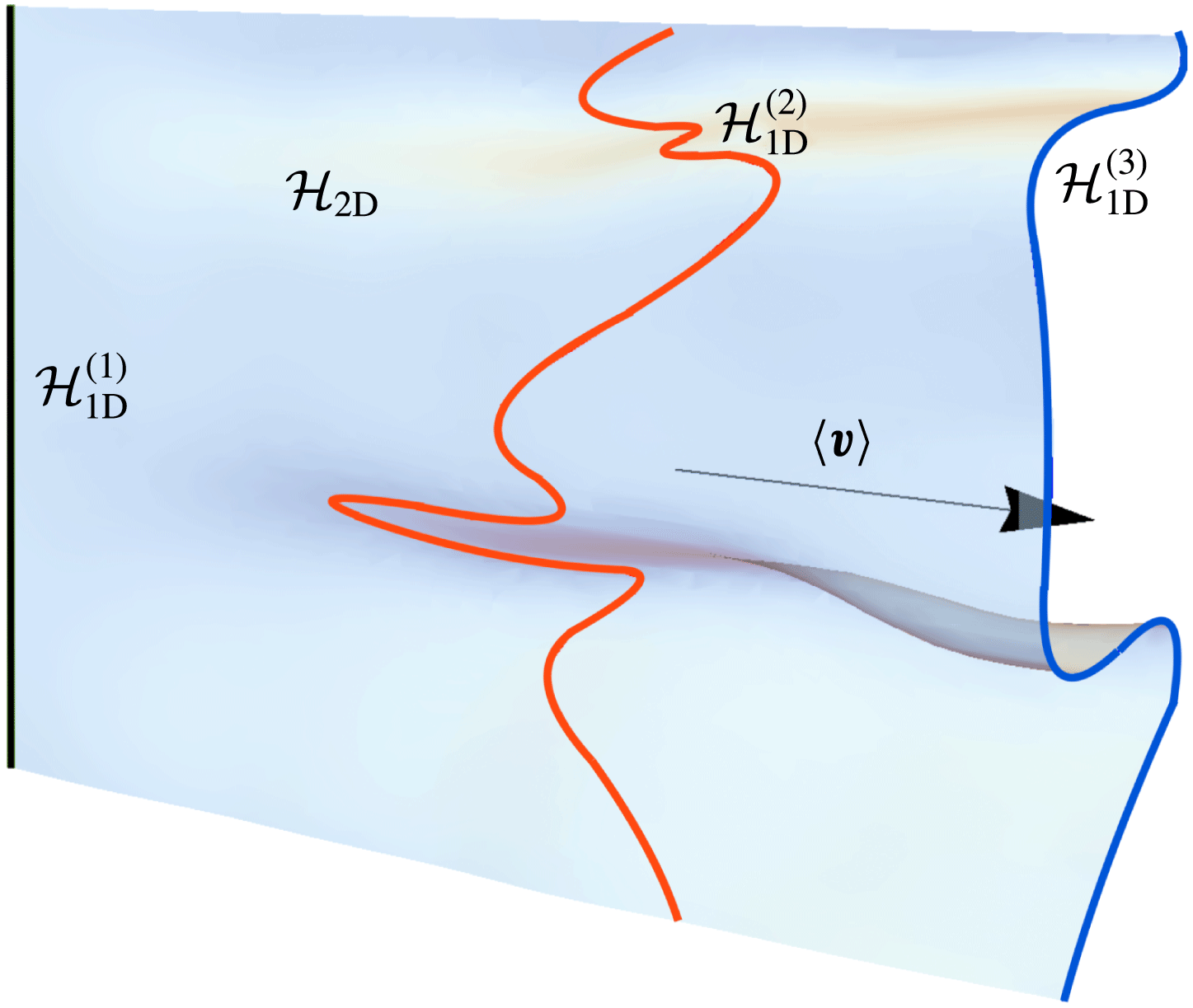
Evolution of a two-dimensional (2-D) material surface
 ${\mathcal{H}}_{2\text{D}}$
(light grey sheet, blue online) with the mean flow direction
 $\langle \boldsymbol{v}\rangle$
(black arrow) arising from a continuously injected 1-D line source
 ${\mathcal{H}}_{1\text{D}}^{(1)}$
(black line). A 1-D cross-section
 ${\mathcal{H}}_{1\text{D}}^{(3)}$
(dark grey line, blue online) of this surface is only subject to transverse deformation, whereas a pulsed injection along
 ${\mathcal{H}}_{1\text{D}}^{(1)}$
subsequently forms the 1-D line
 ${\mathcal{H}}_{1\text{D}}^{(2)}$
(light grey line, red online) which is subject to both transverse and longitudinal fluid deformation.
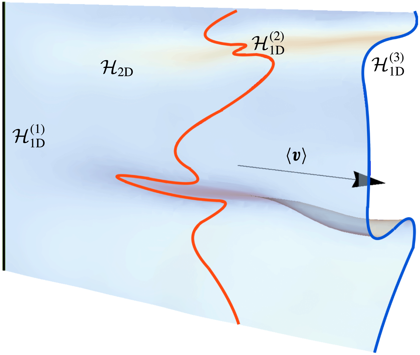
This difference in deformation dynamics is illustrated by the evolution of material elements in the mean translational flow shown in figure 1. Here a continuously injected material line
 ${\mathcal{H}}_{1\text{D}}^{(1)}$
(green line) evolves with the mean flow direction
 $\langle \boldsymbol{v}\rangle$
to form the steady two-dimensional (2-D) material sheet
 ${\mathcal{H}}_{2\text{D}}$
, the cross-section of which
 ${\mathcal{H}}_{1\text{D}}^{(3)}$
(blue line) can evolve into a complex lamellar shape due to fluid deformation transverse to the mean velocity field. In contrast, if we consider the material line
 ${\mathcal{H}}_{1\text{D}}^{(1)}$
to be instantaneously injected at the inlet plane, this line evolves into the 1-D material line
 ${\mathcal{H}}_{1\text{D}}^{(2)}$
(red line) which resides within the 2-D surface
 ${\mathcal{H}}_{2\text{D}}$
. The line
 ${\mathcal{H}}_{1\text{D}}^{(2)}$
deforms due to fluid deformation parallel to the local flow direction, leading to the fingering pattern observed in figure 1, whereas
 ${\mathcal{H}}_{1\text{D}}^{(3)}$
evolves solely due to stretching transverse to the mean flow direction.
We denote fluid deformation in the longitudinal and transverse directions as
 $\unicode[STIX]{x1D6EC}_{l}$
,
 $\unicode[STIX]{x1D6EC}_{t}$
respectively, which directly govern longitudinal and transverse mixing and dispersion. In steady 2-D flow, deformation transverse to the local flow direction (
 $\unicode[STIX]{x1D6EC}_{t}$
) only fluctuates with time, whilst longitudinal deformation (
 $\unicode[STIX]{x1D6EC}_{l}$
) can grow without bound (Attinger, Dentz & Kinzelbach Reference Attinger, Dentz and Kinzelbach2004). Due to the steady flow constraint, fluid deformation evolves via different mechanisms depending upon whether it is parallel or transverse to the local velocity direction. These differences mean that in general, fluid deformation in steady 3-D flows cannot be described in terms of a single scalar quantity (such as mean stretching rate).
As such, models of fluid mixing longitudinal and transverse to the mean flow must reference appropriate components of the fluid deformation tensor, and these can have very different evolution rates. For example, Le Borgne, Dentz & Villermaux (Reference Le Borgne, Dentz and Villermaux2013, Reference Le Borgne, Dentz and Villermaux2015) show that longitudinal deformation
 $\unicode[STIX]{x1D6EC}_{l}$
governs mixing of a pulsed tracer injection in steady 2-D Darcy flow. Conversely, Lester, Dentz & Le Borgne (Reference Lester, Dentz and Le Borgne2016) illustrate that transverse fluid deformation
 $\unicode[STIX]{x1D6EC}_{t}$
governs mixing of a continuously injected source in a steady 3-D flow at the pore scale, and Cirpka et al. (Reference Cirpka, de Barros, Chiogna, Rolle and Nowak2011) show that the same holds for continuously injected sources in two dimensions at the Darcy scale.
In contrast, the unsteady nature of turbulent flows means that the deformation dynamics is largely isotropic with respect to the flow direction, whilst quantities such as vorticity tend to align with principal strain directions (Meneveau Reference Meneveau2011). As a result, stochastic modelling of material deformation has focused on the measurement and development of stochastic models for orientation-invariant measures of deformation, typically in terms of invariants of the strain rate and velocity gradient tensors (Meneveau Reference Meneveau2011; Thalabard et al. Reference Thalabard, Krstulovic and Bec2014). Hence these models are not capable of resolving the constraints associated with steady flows. Conversely, whilst deformation in steady flow has been the subject of a number of studies (Adachi Reference Adachi1983; Finnigan Reference Finnigan1983; Adachi Reference Adachi1986; Finnigan Reference Finnigan, Moffat and Tsinober1990; Tabor Reference Tabor1992), the development of stochastic models of deformation in these flows is an outstanding problem.
To address this shortcoming, in this study we derive an ab initio stochastic model of fluid deformation in steady, random 3-D flows that fully resolve the longitudinal
 $\unicode[STIX]{x1D6EC}_{l}$
and transverse
 $\unicode[STIX]{x1D6EC}_{t}$
deformations. Rather than develop empirical models of fluid deformation in specific flows, we analyse the kinematics of deformation in steady 3-D flows and derive a generic framework applicable to all such flows. This stochastic model takes the form of a coupled continuous-time random walk (CTRW) along fluid streamlines, and represents an extension of previous work by Dentz et al. (Reference Dentz, Lester, Borgne and de Barros2016b
) on stochastic modelling of fluid deformation in steady 2-D flows.
We apply this model to several model flows and show that it accurately resolves the deformation dynamics and provides a valuable link between the Eulerian flow properties and Lagrangian deformation structure. As this CTRW model may be readily applied to existent numerical or experimental datasets, it provides a means to fully characterise and predict Lagrangian fluid deformation in complex steady flows from the Eulerian velocity and velocity gradient statistics. In the context of porous media flow (e.g. pore- and Darcy-scale flow simulations or experiments) this link provides an important building block for the development of fluid transport, mixing and reaction models which may be couched directly in terms of medium properties, such as heterogeneity controls in Darcy-scale flow (e.g. de Barros et al. Reference de Barros, Dentz, Koch and Nowak2012; Le Borgne et al. Reference Le Borgne, Dentz and Villermaux2015).
To begin we first outline the stochastic modelling approach utilised in this study in § 2, and identify a moving streamline coordinate frame, termed a Protean frame, to couch this model. In § 3 we consider evolution of fluid deformation in the Protean frame and derive expressions for evolution of the deformation tensor components in this frame. In § 4 we derive and solve the coupled CTRW model for fluid deformation in the Protean frame coordinates and apply the stochastic model to several model steady flows. In § 5 the velocity and velocity gradient statistics of several model flows in the Protean frame are examined, and model predictions are compared with direct computations. These results are discussed and then conclusions are made in § 6.
2 Stochastic modelling of fluid deformation in steady flows
Steady flows, whether in two or three dimensions, involve topological and kinematic constraints (Tabor Reference Tabor1992) which impact the deformation of material elements. To develop a general stochastic modelling framework which honours these constraints, it is necessary to resolve the deformation tensor in a frame relative to the local velocity field. By utilising a coordinate frame which aligns with the streamlines of the flow, the topological constraints upon fluid deformation associated with steady flow are automatically imposed, and the stretching and shear contributions to deformation are clearly resolved. Specifically, we seek to develop stochastic models for the evolution of
 $\unicode[STIX]{x1D6EC}_{t}$
and
 $\unicode[STIX]{x1D6EC}_{l}$
in various flow regimes and across time scales which observe these kinematic constraints.
There exist several choices for streamline coordinate frames in steady flows, ranging from moving Cartesian coordinate frames to curvilinear streamline coordinate systems and convected coordinates. Adachi (Reference Adachi1983, Reference Adachi1986) presents a rotating Cartesian coordinate frame, termed a Protean coordinate frame, to study fluid deformation in 2-D planar and axisymmetric flows. Similar to other streamline coordinate frames (such as Frenet–Serret coordinates (Finnigan Reference Finnigan, Moffat and Tsinober1990) or curvilinear streamline coordinates), this frame automatically imposes the topological and kinematic constraints outlined in § 1 that are inherent to steady flows.
In contrast to these coordinate systems, the moving Protean coordinate frame renders the velocity gradient tensor upper triangular. As shown in appendix B, orthogonal streamline coordinate systems do not possess this property, and moreover it appears difficult to define a consistent streamline coordinate system for chaotic flows (Finnigan Reference Finnigan, Moffat and Tsinober1990). The upper triangular form of the velocity gradient in the Protean frame greatly simplifies solution of the deformation gradient tensor, which may now be expressed in terms of definite integrals of the velocity gradient components (Adachi Reference Adachi1983, Reference Adachi1986). This representation then facilitates the development of stochastic models of fluid deformation, based upon solution of these integrals as a random walk process along fluid streamlines. Dentz et al. (Reference Dentz, Lester, Borgne and de Barros2016b ) used the Protean frame as the basis for the development of a stochastic model of fluid deformation in random steady 2-D flows. In this study we are concerned with the extension of this approach to random steady 3-D flow.
Unlike steady 2-D flow, the moving streamline coordinate frame is not unique for steady 3-D flow due to the additional degree of freedom associated with orientation of the frame about a streamline. As will be shown in § 3.2, the velocity gradient tensor is also no longer upper triangular for any arbitrary orientation about a streamline. However, we extend the Protean coordinate frame of Adachi (Reference Adachi1983, Reference Adachi1986) to arbitrary steady 3-D flows by choosing the orientation angle that renders the velocity gradient upper triangular, recovering the integral solutions for the deformation tensor components. In some sense this 3-D Protean frame for calculating fluid deformation in steady flow is analogous to continuous QR decomposition methods (Dieci, Russell & Van Vleck Reference Dieci, Russell and Van Vleck1997; Dieci & Vleck Reference Dieci and Van Vleck2008) for autonomous dynamical systems, which automatically recover constraints such as regularity and volume preservation of phase space.
In contrast to 2-D flow, 3-D steady flow also admits the possibility of chaotic fluid trajectories and exponential fluid deformation. In this context, an appropriate framework is needed which can also correctly capture either the Lyapunov exponents (exponential stretching rates) associated with chaotic flows or the power-law indices associated with algebraic fluid stretching in non-chaotic flows (such as isotropic Darcy flow). In § 3.2 we show that the ensemble average of the diagonal components of the velocity gradient in the Protean frame correspond directly to the Lyapunov exponents of the flow. With respect to non-chaotic flows, special care is also required to suppress spurious exponential stretching in stochastic models, even for steady 2-D flows. For example, Duplat, Innocenti & Villermaux (Reference Duplat, Innocenti and Villermaux2010) discuss a series of stretching mechanisms to explain observed sub-exponential (algebraic) stretching across a broad range of flow. Rather, algebraic stretching is inherent to steady 2-D flow as a direct result of the topological constraints of these flows (associated with the Poincaré–Bendixson theorem). Dentz et al. (Reference Dentz, Lester, Borgne and de Barros2016b ) show that the use of streamline coordinates for 2-D flows automatically recovers these constraints without resort to any specialised stretching mechanism. In appendix B we show that certain components of the velocity gradient tensor are rendered zero for non-chaotic 3-D flows such as complex lamellar (Finnigan Reference Finnigan1983; Kelvin Reference Kelvin1884) or zero-helicity-density (Moffatt Reference Moffatt1969) flows, automatically recovering the kinematic constraints associated with these steady flows. Hence the Protean frame automatically adheres to the topological and kinematic constraints associated with chaotic and non-chaotic steady flows, so seems well suited to the development of stochastic models of fluid deformation in these flows.
In steady random flows, Lagrangian velocities along streamlines fluctuate on a scale set by the random flow spatial structure. Hence, both the fluid velocity and velocity gradient tend to follow a spatial Markov process along streamlines (Le Borgne, Dentz & Carrera Reference Le Borgne, Dentz and Carrera2008a ,Reference Le Borgne, Dentz and Carrera b ), as these properties decorrelate in space. By exploiting this property and the Protean coordinate frame, we derive a stochastic deformation model in steady random flows as a coupled continuous-time random walk (CTRW). The CTRW framework allows accounting for the broad velocity distributions that characterise steady random flows and lead to anomalous transport behaviour (Dentz et al. Reference Dentz, Kang, Comolli, Le Borgne and Lester2016a ). A similar approach has been applied previously by Dentz et al. (Reference Dentz, Lester, Borgne and de Barros2016b ) to steady 2-D flows, leading to significant insights into the mechanisms which control fluid deformation in steady flow, namely that fluid deformation evolves as a coupled Lévy process due to the coupling between shear deformation and velocity fluctuations along streamlines.
For 3-D flows, the possibility of exponential fluid stretching augments the couplings between shear, stretching, velocity and deformation leading to wholly new deformation dynamics in steady 3-D flows, which is captured by the presented CTRW model. By solving this CTRW model, we can then make quantitative predictions of longitudinal
 $\unicode[STIX]{x1D6EC}_{l}$
and transverse
 $\unicode[STIX]{x1D6EC}_{t}$
fluid deformation in steady 3-D random flows from statistical characterisation of the fluid velocity and velocity gradients. This facilitates the quantification of fluid deformation (and hence mixing, reaction and dispersion) directly from e.g. experimental or computational flow datasets. We begin by consideration of fluid deformation in the Protean frame.
3 Fluid deformation in the Protean coordinate frame
In this section we extend the Protean coordinate frame of Adachi (Reference Adachi1983, Reference Adachi1986) to 3-D steady flows and derive the evolution equations for the deformation gradient in streamline coordinates.
3.1 General development
The evolution of the location
 $\boldsymbol{x}(t)$
of fluid element in the steady spatially heterogeneous flow field
 $\boldsymbol{u}(\boldsymbol{x})$
is given by the advection equation
 $$\begin{eqnarray}\frac{\text{d}\boldsymbol{x}(t;\boldsymbol{X})}{\text{d}t}=\boldsymbol{v}(t),\quad \boldsymbol{v}(t;\boldsymbol{X})\equiv \boldsymbol{u}[\boldsymbol{x}(t;\boldsymbol{X})],\end{eqnarray}$$
where we denote the reference material vectors in the Eulerian and Lagrangian frames by
 $\boldsymbol{x}(t)$
and
 $\boldsymbol{X}$
, respectively. The deformation gradient tensor
 $\unicode[STIX]{x1D641}(t)$
quantifies how the infinitesimal vector
 $\text{d}\boldsymbol{x}(t;\boldsymbol{X})$
deforms from its reference state
 $\text{d}\boldsymbol{x}(t=0;\boldsymbol{X})=\text{d}\boldsymbol{X}$
as
 $$\begin{eqnarray}\text{d}\boldsymbol{x}=\unicode[STIX]{x1D641}(t)\boldsymbol{\cdot }\text{d}\boldsymbol{X}\end{eqnarray}$$
and equivalently
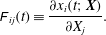 $$\begin{eqnarray}\unicode[STIX]{x1D60D}_{ij}(t)\equiv \frac{\unicode[STIX]{x2202}x_{i}(t;\boldsymbol{X})}{\unicode[STIX]{x2202}X_{j}}.\end{eqnarray}$$
Following this definition, the deformation gradient tensor
 $\unicode[STIX]{x1D641}(t)$
evolves with travel time
 $t$
along a Lagrangian trajectory (streamline) as
 $$\begin{eqnarray}\frac{\text{d}\unicode[STIX]{x1D641}(t)}{\text{d}t}=\unicode[STIX]{x1D750}(t)\unicode[STIX]{x1D641}(t),\quad \unicode[STIX]{x1D641}(0)=\mathbf{1},\end{eqnarray}$$
where the velocity gradient tensor
 $\unicode[STIX]{x1D750}(t)=\unicode[STIX]{x1D735}\boldsymbol{v}(t)^{\top }\equiv \unicode[STIX]{x1D735}\boldsymbol{u}[\boldsymbol{x}(t;\boldsymbol{X})]^{\top }$
and the superscript
 $\top$
denotes the transpose. Rather than use a curvilinear streamline coordinate system, we consider the transform of a fixed orthogonal Cartesian coordinate system into the Protean coordinate frame which consists of moving Cartesian coordinates. We denote spatial coordinates in the fixed Cartesian coordinate system as
 $\boldsymbol{x}=(x_{1},x_{2},x_{3})^{\top }$
, and the reoriented Protean coordinate system by
 $\boldsymbol{x}^{\prime }=(x_{1}^{\prime },x_{2}^{\prime },x_{3}^{\prime })^{\top }$
, where the velocity vector
 $\boldsymbol{v}(\boldsymbol{x})=(v_{1},v_{2},v_{3})^{\top }$
in the Cartesian frame transforms to
 $\boldsymbol{v}^{\prime }(\boldsymbol{x}^{\prime })=(v,0,0)^{\top }$
in the Protean frame, with
 $v=|\boldsymbol{v}|$
. These two frames are related by the transform (Truesdell & Noll Reference Truesdell and Noll1992)
 $$\begin{eqnarray}\boldsymbol{x}^{\prime }=\boldsymbol{x}_{0}(t)+\unicode[STIX]{x1D64C}^{\top }(t)\boldsymbol{x},\end{eqnarray}$$
where
 $\boldsymbol{x}_{0}(t)$
is an arbitrary translation vector, and
 $\unicode[STIX]{x1D64C}(t)$
is a rotation matrix (or proper orthogonal transformation):
 $\unicode[STIX]{x1D64C}^{\top }(t)\boldsymbol{\cdot }\unicode[STIX]{x1D64C}(t)=\mathbf{1}$
,
 $\det [\unicode[STIX]{x1D64C}(t)]=1$
. From (3.5) the differential elements
 $\text{d}\boldsymbol{x}$
,
 $\text{d}\boldsymbol{X}$
transform respectively as
 $\text{d}\boldsymbol{x}^{\prime }=\unicode[STIX]{x1D64C}^{\top }(t)\,\text{d}\boldsymbol{x}$
,
 $\text{d}\boldsymbol{X}^{\prime }=\unicode[STIX]{x1D64C}^{\top }(0)\,\text{d}\boldsymbol{X}$
, and so from (3.2) the deformation gradient tensor then transforms as
 $$\begin{eqnarray}\unicode[STIX]{x1D641}^{\prime }(t)=\unicode[STIX]{x1D64C}^{\top }(t)\unicode[STIX]{x1D641}(t)\unicode[STIX]{x1D64C}(0).\end{eqnarray}$$
Formally,
 $\unicode[STIX]{x1D641}(t)$
is a pseudo-tensor (Truesdell & Noll Reference Truesdell and Noll1992), as it is not objective as per (3.6),
 $\unicode[STIX]{x1D641}^{\prime }(t)\neq \unicode[STIX]{x1D64C}^{\top }(t)\unicode[STIX]{x1D641}(t)\unicode[STIX]{x1D64C}(t)$
(Ottino Reference Ottino1989). Differentiating (3.6) with respect to the Lagrangian travel time
 $t$
yields
 $$\begin{eqnarray}\frac{\text{d}\unicode[STIX]{x1D641}^{\prime }}{\text{d}t}=\dot{\unicode[STIX]{x1D64C}}^{\top }(t)\unicode[STIX]{x1D641}(t)\unicode[STIX]{x1D64C}(0)+\unicode[STIX]{x1D64C}^{\top }(t)\unicode[STIX]{x1D750}(t)\unicode[STIX]{x1D641}(t)\unicode[STIX]{x1D64C}(0)=\unicode[STIX]{x1D750}^{\prime }(t)\unicode[STIX]{x1D641}^{\prime }(t),\end{eqnarray}$$
where the transformed rate of strain tensor
 $\unicode[STIX]{x1D750}^{\prime }(t)$
is defined as
 $$\begin{eqnarray}\unicode[STIX]{x1D750}^{\prime }(t)\equiv \unicode[STIX]{x1D64C}^{\top }(t)\unicode[STIX]{x1D750}(t)\unicode[STIX]{x1D64C}(t)+\unicode[STIX]{x1D63C}(t),\end{eqnarray}$$
and the contribution due to a moving coordinate frame is
 $\unicode[STIX]{x1D63C}(t)\equiv \dot{\unicode[STIX]{x1D64C}}^{\top }(t)\unicode[STIX]{x1D64C}(t)$
. As
 $\unicode[STIX]{x1D64C}(t)$
is orthogonal, then
 $\dot{\unicode[STIX]{x1D64C}}^{\top }(t)\unicode[STIX]{x1D64C}(t)+\unicode[STIX]{x1D64C}^{\top }(t)\dot{\unicode[STIX]{x1D64C}}(t)=0$
and so
 $\unicode[STIX]{x1D63C}(t)$
is skew-symmetric. Note that the velocity vector
 $\boldsymbol{v}(t)=\text{d}\boldsymbol{x}/\text{d}t$
also transforms as
 $\boldsymbol{v}^{\prime }(t)=\unicode[STIX]{x1D64C}^{\top }(t)\boldsymbol{v}(t)$
. The basic idea of the Protean coordinate frame is to find an appropriate local reorientation
 $\unicode[STIX]{x1D64C}(t)$
that renders the transformed velocity gradient
 $\unicode[STIX]{x1D750}^{\prime }(t)$
upper triangular, simplifying solution of the deformation tensor
 $\unicode[STIX]{x1D641}$
in (3.7).
3.2 Fluid deformation in 3-D Protean coordinates
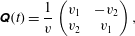
Adachi (Reference Adachi1983, Reference Adachi1986) shows that for steady 2-D flow, reorientation into streamline coordinates automatically yields an upper triangular velocity gradient tensor, hence the reorientation matrix
 $\unicode[STIX]{x1D64C}(t)$
is simply given in terms of the velocity
 $\boldsymbol{v}=[v_{1},v_{2}]^{\top }$
in the fixed Cartesian frame as
 $$\begin{eqnarray}\unicode[STIX]{x1D64C}(t)=\frac{1}{v}\left(\begin{array}{@{}cc@{}}v_{1} & -v_{2}\\ v_{2} & v_{1}\end{array}\right),\end{eqnarray}$$
hence
 $\boldsymbol{v}^{\prime }=[v,0]^{\top }$
, where
 $v=\sqrt{v_{1}^{2}+v_{2}^{2}}$
.
In contrast to steady 2-D flow, the additional spatial dimension of steady 3-D flows admits an additional degree of freedom for the specification of streamline coordinates. In 3-D streamline coordinates, the base vector
 $\boldsymbol{e}_{1}^{\prime }(t)$
aligns with the velocity vector
 $\boldsymbol{v}(t)$
, such that
 $\boldsymbol{v}^{\prime }(t)=[v(t),0,0]^{\top }$
, but the transverse vectors
 $\boldsymbol{e}_{2}^{\prime }(t)$
and
 $\boldsymbol{e}_{3}^{\prime }(t)$
are arbitrary up to a rotation about
 $\boldsymbol{e}_{1}^{\prime }(t)$
. As these base vectors are not material coordinates, this degree of freedom does not impact the governing kinematics.
For the Protean coordinate frame it is required to reorient the rate of strain tensor
 $\unicode[STIX]{x1D750}^{\prime }(t)$
such that it is upper triangular, yielding explicit closed-form solution for the deformation gradient tensor
 $\unicode[STIX]{x1D641}^{\prime }(t)$
and elucidating the deformation dynamics. Whilst all square matrices are unitarily similar (mathematically equivalent) to an upper triangular matrix, it is unclear whether such a similarity transform is orthogonal, or corresponds to a reorientation of frame, or indeed corresponds to a reorientation into streamline coordinates. As demonstrated by Adachi (Reference Adachi1983, Reference Adachi1986), this condition is satisfied for all steady 2-D flows, but this is still an open question for steady 3-D flows.
For reasons that will become apparent, we develop the 3-D Protean coordinate frame by decomposing the reorientation matrix
 $\unicode[STIX]{x1D64C}(t)$
into two sequential reorientations
 $\unicode[STIX]{x1D64C}_{1}(t)$
,
 $\unicode[STIX]{x1D64C}_{2}(t)$
as
 $$\begin{eqnarray}\unicode[STIX]{x1D64C}(t)\equiv \unicode[STIX]{x1D64C}_{2}(t)\unicode[STIX]{x1D64C}_{1}(t),\end{eqnarray}$$
where
 $\unicode[STIX]{x1D64C}_{1}(t)$
is a reorientation that aligns the velocity vector
 $\boldsymbol{v}$
with the Protean base vector
 $\boldsymbol{e}_{1}^{\prime }(t)$
, and
 $\unicode[STIX]{x1D64C}_{2}(t)$
is a subsequent reorientation of the Protean frame about
 $\boldsymbol{e}_{1}^{\prime }(t)$
. As such, the reorientation
 $\unicode[STIX]{x1D64C}_{1}(t)$
renders the Protean frame a streamline coordinate frame, and
 $\unicode[STIX]{x1D64C}_{2}$
represents a (currently) arbitrary reorientation of this streamline frame about the velocity vector.
We begin by considering the 3-D rotation matrix
 $\unicode[STIX]{x1D64C}_{1}(t)$
which is defined in terms of the unit rotation axis
 $\boldsymbol{q}(t)$
(which is orthogonal to both the velocity and
 $\boldsymbol{e}_{1}$
vectors), and the associated reorientation angle
 $\unicode[STIX]{x1D703}(t)$
, both of which are given in terms of the local velocity vector
 $\boldsymbol{v}(t)=[v_{1},v_{2},v_{3}]^{\top }$
as
 $$\begin{eqnarray}\displaystyle & \displaystyle \boldsymbol{q}(t)=\frac{\boldsymbol{e}_{1}\times \boldsymbol{v}}{\Vert \boldsymbol{e}_{1}\times \boldsymbol{v}\Vert }=\frac{1}{\sqrt{v_{2}^{2}+v_{3}^{2}}}\{0,v_{3},-v_{2}\}, & \displaystyle\end{eqnarray}$$
 $$\begin{eqnarray}\displaystyle & \displaystyle \cos \unicode[STIX]{x1D703}(t)=\frac{\boldsymbol{e}_{1}\boldsymbol{\cdot }\boldsymbol{v}}{\Vert \boldsymbol{e}_{1}\boldsymbol{\cdot }\boldsymbol{v}\Vert }=\frac{v_{1}}{v}. & \displaystyle\end{eqnarray}$$
The rotation tensor
 $\unicode[STIX]{x1D64C}_{1}(t)$
then is given by
 $$\begin{eqnarray}\unicode[STIX]{x1D64C}_{1}(t)=\cos \unicode[STIX]{x1D703}(t)\unicode[STIX]{x1D644}+\sin \unicode[STIX]{x1D703}(t)(\boldsymbol{q})_{\times }^{\top }+[1-\cos \unicode[STIX]{x1D703}(t)]\boldsymbol{q}(t)\otimes \boldsymbol{q}(t),\end{eqnarray}$$
where
 $\unicode[STIX]{x1D644}$
is the identity matrix,
 $(\cdot )_{\times }$
denotes the cross-product matrix and
 $\Vert \cdot \Vert$
is the
 $\ell ^{2}$
-norm. The second reorientation matrix
 $\unicode[STIX]{x1D64C}_{2}(t)$
corresponds to an arbitrary reorientation (of angle
 $\unicode[STIX]{x1D6FC}(t)$
) about the
 $\boldsymbol{e}_{1}^{\prime }$
axis, which is explicitly
 $$\begin{eqnarray}\unicode[STIX]{x1D64C}_{2}(t)=\left(\begin{array}{@{}ccc@{}}1 & 0 & 0\\ 0 & \cos \unicode[STIX]{x1D6FC}(t) & -\text{sin}\,\unicode[STIX]{x1D6FC}(t)\\ 0 & \sin \unicode[STIX]{x1D6FC}(t) & \cos \unicode[STIX]{x1D6FC}(t)\end{array}\right).\end{eqnarray}$$
Whilst the algebraic expressions (in terms of
 $\unicode[STIX]{x1D6FC}$
,
 $v_{1}$
,
 $v_{2}$
,
 $v_{3}$
) for the components of the composition rotation matrix
 $\unicode[STIX]{x1D64C}(t)=\unicode[STIX]{x1D64C}_{2}(t)\unicode[STIX]{x1D64C}_{1}(t)$
are somewhat complicated, it is useful to note that
 $\unicode[STIX]{x1D64C}(t)$
may be expressed in terms of the Protean frame basis vectors as
 $$\begin{eqnarray}\unicode[STIX]{x1D64C}(t)=[\boldsymbol{e}_{1}^{\prime }(t),\boldsymbol{e}_{2}^{\prime }(t),\boldsymbol{e}_{3}^{\prime }(t)],\end{eqnarray}$$
hence the moving coordinate contribution
 $\unicode[STIX]{x1D63C}(t)$
is given by
 $$\begin{eqnarray}\unicode[STIX]{x1D63C}(t)=\dot{\unicode[STIX]{x1D64C}}^{\top }(t)\unicode[STIX]{x1D64C}(t)=\left(\begin{array}{@{}ccc@{}}0 & \boldsymbol{e}_{2}^{\prime }(t)\boldsymbol{\cdot }\dot{\boldsymbol{e}}_{1}^{\prime }(t) & \boldsymbol{e}_{3}^{\prime }(t)\boldsymbol{\cdot }\dot{\boldsymbol{e}}_{1}^{\prime }(t)\\ -\boldsymbol{e}_{2}^{\prime }(t)\boldsymbol{\cdot }\dot{\boldsymbol{e}}_{1}^{\prime }(t) & 0 & \boldsymbol{e}_{3}^{\prime }(t)\boldsymbol{\cdot }\dot{\boldsymbol{e}}_{2}^{\prime }(t)\\ -\boldsymbol{e}_{3}^{\prime }(t)\boldsymbol{\cdot }\dot{\boldsymbol{e}}_{1}^{\prime }(t) & -\boldsymbol{e}_{3}^{\prime }(t)\boldsymbol{\cdot }\dot{\boldsymbol{e}}_{2}^{\prime }(t) & 0\end{array}\right).\end{eqnarray}$$
Defining the Protean velocity gradient in the absence of this contribution as
 $\tilde{\unicode[STIX]{x1D750}}(t)$
,
 $$\begin{eqnarray}\tilde{\unicode[STIX]{x1D750}}(t)\equiv \unicode[STIX]{x1D64C}^{\top }(t)\unicode[STIX]{x1D750}(t)\unicode[STIX]{x1D64C}(t)=\unicode[STIX]{x1D750}^{\prime }(t)-\unicode[STIX]{x1D63C}(t),\end{eqnarray}$$
we find the components of
 $\unicode[STIX]{x1D63C}(t)$
may be related to
 $\tilde{\unicode[STIX]{x1D750}}(t)$
as follows. From (3.17) and (3.15),
 $\tilde{\unicode[STIX]{x1D716}}_{ij}(t)=\boldsymbol{e}_{i}^{\prime }(t)\unicode[STIX]{x1D750}(t)\boldsymbol{e}_{j}^{\prime }(t)$
, and since
 $\dot{\boldsymbol{v}}(t)=\unicode[STIX]{x1D750}(t)\boldsymbol{\cdot }\boldsymbol{v}(t)$
,
 $\boldsymbol{e}_{1}^{\prime }(t)=\boldsymbol{v}(t)/v(t)$
, then
 $$\begin{eqnarray}\displaystyle & \displaystyle \boldsymbol{e}_{2}^{\prime }(t)\boldsymbol{\cdot }\dot{\boldsymbol{e}}_{1}^{\prime }(t)=\boldsymbol{e}_{2}^{\prime }(t)\boldsymbol{\cdot }\unicode[STIX]{x1D750}(t)\boldsymbol{\cdot }\boldsymbol{e}_{1}^{\prime }(t)=\tilde{\unicode[STIX]{x1D716}}_{21}(t), & \displaystyle\end{eqnarray}$$
 $$\begin{eqnarray}\displaystyle & \displaystyle \boldsymbol{e}_{3}^{\prime }(t)\boldsymbol{\cdot }\dot{\boldsymbol{e}}_{1}^{\prime }(t)=\boldsymbol{e}_{3}^{\prime }(t)\boldsymbol{\cdot }\unicode[STIX]{x1D716}(t)\boldsymbol{\cdot }\boldsymbol{e}_{1}^{\prime }(t)=\tilde{\unicode[STIX]{x1D716}}_{31}(t). & \displaystyle\end{eqnarray}$$
From these relationships the Protean velocity gradient tensor
 $\unicode[STIX]{x1D750}^{\prime }(t)=\tilde{\unicode[STIX]{x1D750}}+\unicode[STIX]{x1D63C}(t)$
is then
 $$\begin{eqnarray}\unicode[STIX]{x1D750}^{\prime }(t)=\left(\begin{array}{@{}ccc@{}}\tilde{\unicode[STIX]{x1D716}}_{11} & \tilde{\unicode[STIX]{x1D716}}_{12}+\tilde{\unicode[STIX]{x1D716}}_{21} & \tilde{\unicode[STIX]{x1D716}}_{13}+\tilde{\unicode[STIX]{x1D716}}_{31}\\ 0 & \tilde{\unicode[STIX]{x1D716}}_{22} & \tilde{\unicode[STIX]{x1D716}}_{23}+\unicode[STIX]{x1D608}_{23}(t)\\ 0 & \tilde{\unicode[STIX]{x1D716}}_{32}-\unicode[STIX]{x1D608}_{23}(t) & -\tilde{\unicode[STIX]{x1D716}}_{22}-\tilde{\unicode[STIX]{x1D716}}_{11}\end{array}\right),\end{eqnarray}$$
where
 $\unicode[STIX]{x1D608}_{23}(t)=\boldsymbol{e}_{3}^{\prime }(t)\boldsymbol{\cdot }\dot{\boldsymbol{e}}_{2}^{\prime }(t)$
. As the reorientation
 $\unicode[STIX]{x1D64C}_{2}$
(3.14) only impacts the
 $\unicode[STIX]{x1D716}_{22}^{\prime }$
,
 $\unicode[STIX]{x1D716}_{23}^{\prime }$
,
 $\unicode[STIX]{x1D716}_{32}^{\prime }$
,
 $\unicode[STIX]{x1D716}_{33}^{\prime }$
components, reorientation (via
 $\unicode[STIX]{x1D64C}_{1}(t)$
) into streamline coordinates automatically renders the
 $\unicode[STIX]{x1D716}_{21}^{\prime }$
,
 $\unicode[STIX]{x1D716}_{31}^{\prime }$
components of the velocity gradient tensor zero. It is this transform which renders the Protean velocity gradient upper triangular for 2-D steady flows.
Whilst
 $\unicode[STIX]{x1D716}_{32}^{\prime }=\tilde{\unicode[STIX]{x1D716}}_{32}-\unicode[STIX]{x1D608}_{23}$
is non-zero in general,
 $\unicode[STIX]{x1D750}^{\prime }(t)$
may be rendered upper triangular by appropriate manipulation of the arbitrary reorientation angle
 $\unicode[STIX]{x1D6FC}(t)$
such that
 $\unicode[STIX]{x1D608}_{23}=\tilde{\unicode[STIX]{x1D716}}_{32}$
. In a similar manner to (3.18), (3.19), we may express
 $\unicode[STIX]{x1D608}_{23}$
in terms of the components of
 $\unicode[STIX]{x1D750}(t)$
as
 $$\begin{eqnarray}\boldsymbol{e}_{3}^{\prime }(t)\boldsymbol{\cdot }\dot{\boldsymbol{e}}_{2}^{\prime }(t)=v(t)\boldsymbol{e}_{3}^{\prime }(t)\left[\frac{\unicode[STIX]{x2202}\boldsymbol{e}_{2}^{\prime }(t)}{\unicode[STIX]{x2202}\boldsymbol{v}}\unicode[STIX]{x1D750}(t)\right]\boldsymbol{e}_{1}^{\prime }(t)+\boldsymbol{e}_{3}^{\prime }(t)\boldsymbol{\cdot }\frac{\unicode[STIX]{x2202}\boldsymbol{e}_{2}^{\prime }(t)}{\unicode[STIX]{x2202}\unicode[STIX]{x1D6FC}(t)}\frac{\text{d}\unicode[STIX]{x1D6FC}}{\text{d}t},\end{eqnarray}$$
 $$\begin{eqnarray}\displaystyle & \displaystyle v\boldsymbol{e}_{3}^{\prime }\boldsymbol{\cdot }\frac{\unicode[STIX]{x2202}\boldsymbol{e}_{2}^{\prime }}{\unicode[STIX]{x2202}\boldsymbol{v}}=\frac{1}{v+v_{1}}\{0,v_{3},-v_{2}\}=\frac{v_{3}\cos \unicode[STIX]{x1D6FC}-v_{2}\sin \unicode[STIX]{x1D6FC}}{v+v_{1}}\boldsymbol{e}_{2}^{\prime }-\frac{v_{2}\cos \unicode[STIX]{x1D6FC}+v_{3}\sin \unicode[STIX]{x1D6FC}}{v+v_{1}}\boldsymbol{e}_{3}^{\prime },\qquad & \displaystyle\end{eqnarray}$$
 $$\begin{eqnarray}\displaystyle & \displaystyle \boldsymbol{e}_{3}^{\prime }\boldsymbol{\cdot }\frac{\unicode[STIX]{x2202}\boldsymbol{e}_{2}^{\prime }}{\unicode[STIX]{x2202}\unicode[STIX]{x1D6FC}}=-1, & \displaystyle\end{eqnarray}$$
and so
 $\unicode[STIX]{x1D608}_{23}(t)$
is then
 $$\begin{eqnarray}\unicode[STIX]{x1D608}_{23}(t)=\boldsymbol{e}_{3}^{\prime }\boldsymbol{\cdot }\dot{\boldsymbol{e}}_{2}^{\prime }=\frac{v_{3}\cos \unicode[STIX]{x1D6FC}-v_{2}\sin \unicode[STIX]{x1D6FC}}{v+v_{1}}\tilde{\unicode[STIX]{x1D716}}_{21}-\frac{v_{2}\cos \unicode[STIX]{x1D6FC}+v_{3}\sin \unicode[STIX]{x1D6FC}}{v+v_{1}}\tilde{\unicode[STIX]{x1D716}}_{31}-\frac{\text{d}\unicode[STIX]{x1D6FC}}{\text{d}t}.\end{eqnarray}$$
Hence the equation
 $\unicode[STIX]{x1D608}_{23}(t)=\tilde{\unicode[STIX]{x1D716}}_{32}$
defines an ordinary differential equation (ODE) for the arbitrary orientation angle
 $\unicode[STIX]{x1D6FC}(t)$
which renders
 $\unicode[STIX]{x1D750}^{\prime }(t)$
upper triangular. Although the components of
 $\tilde{\unicode[STIX]{x1D750}}(t)$
vary with
 $\unicode[STIX]{x1D6FC}$
, these may be expressed in terms of the components of
 $\unicode[STIX]{x1D750}^{(1)}$
(which are independent of
 $\unicode[STIX]{x1D6FC}$
), defined as
 $$\begin{eqnarray}\unicode[STIX]{x1D750}^{(1)}(t)\equiv \unicode[STIX]{x1D64C}_{1}^{\top }(t)\unicode[STIX]{x1D750}(t)\unicode[STIX]{x1D64C}_{1}(t),\end{eqnarray}$$
where the components of
 $\tilde{\unicode[STIX]{x1D750}}(t)$
and
 $\unicode[STIX]{x1D750}^{(1)}(t)$
are related as
 $$\begin{eqnarray}\displaystyle & \displaystyle \tilde{\unicode[STIX]{x1D716}}_{21}=\unicode[STIX]{x1D716}_{21}^{(1)}\cos \unicode[STIX]{x1D6FC}+\unicode[STIX]{x1D716}_{31}^{(1)}\sin \unicode[STIX]{x1D6FC}, & \displaystyle\end{eqnarray}$$
 $$\begin{eqnarray}\displaystyle & \displaystyle \tilde{\unicode[STIX]{x1D716}}_{31}=\unicode[STIX]{x1D716}_{31}^{(1)}\cos \unicode[STIX]{x1D6FC}-\unicode[STIX]{x1D716}_{21}^{(1)}\sin \unicode[STIX]{x1D6FC}, & \displaystyle\end{eqnarray}$$
 $$\begin{eqnarray}\displaystyle & \displaystyle \tilde{\unicode[STIX]{x1D716}}_{32}=\unicode[STIX]{x1D716}_{32}^{(1)}\cos ^{2}\unicode[STIX]{x1D6FC}-\unicode[STIX]{x1D716}_{23}^{(1)}\sin ^{2}\unicode[STIX]{x1D6FC}+(\unicode[STIX]{x1D716}_{33}^{(1)}-\unicode[STIX]{x1D716}_{22}^{(1)})\cos \unicode[STIX]{x1D6FC}\sin \unicode[STIX]{x1D6FC}. & \displaystyle\end{eqnarray}$$
Hence the condition
 $\unicode[STIX]{x1D608}_{23}=\tilde{\unicode[STIX]{x1D716}}_{32}$
is satisfied by the ODE
 $$\begin{eqnarray}\displaystyle \frac{\text{d}\unicode[STIX]{x1D6FC}}{\text{d}t} & = & \displaystyle g(\unicode[STIX]{x1D6FC},t)\nonumber\\ \displaystyle & = & \displaystyle a(t)\cos ^{2}\unicode[STIX]{x1D6FC}+b(t)\sin ^{2}\unicode[STIX]{x1D6FC}+c(t)\cos \unicode[STIX]{x1D6FC}\sin \unicode[STIX]{x1D6FC},\end{eqnarray}$$
where
 $$\begin{eqnarray}\displaystyle & \displaystyle a(t)=-\unicode[STIX]{x1D716}_{32}^{(1)}-\frac{v_{2}}{v+v_{1}}\unicode[STIX]{x1D716}_{31}^{(1)}-\frac{v_{3}}{v+v_{1}}\unicode[STIX]{x1D716}_{21}^{(1)}, & \displaystyle\end{eqnarray}$$
 $$\begin{eqnarray}\displaystyle & \displaystyle b(t)=\unicode[STIX]{x1D716}_{23}^{(1)}+\frac{v_{2}}{v+v_{1}}\unicode[STIX]{x1D716}_{31}^{(1)}+\frac{v_{3}}{v+v_{1}}\unicode[STIX]{x1D716}_{21}^{(1)}, & \displaystyle\end{eqnarray}$$
 $$\begin{eqnarray}\displaystyle & \displaystyle c(t)=\unicode[STIX]{x1D716}_{22}^{(1)}-\unicode[STIX]{x1D716}_{33}^{(1)}+\frac{2v_{2}}{v+v_{1}}\unicode[STIX]{x1D716}_{21}^{(1)}-\frac{2v_{3}}{v+v_{1}}\unicode[STIX]{x1D716}_{31}^{(1)}. & \displaystyle\end{eqnarray}$$
3.2.1 Evolution of Protean orientation angle
 $\unicode[STIX]{x1D6FC}(t)$

Equation (3.29) describes a first-order ODE for the transverse orientation angle
 $\unicode[STIX]{x1D6FC}(t)$
along a streamline which renders
 $\unicode[STIX]{x1D750}^{\prime }(t)$
upper triangular. Here the temporal derivative for
 $\unicode[STIX]{x1D6FC}(t)$
is associated with both change in flow structure along a streamline and impact of a moving coordinate transform as encoded by
 $\unicode[STIX]{x1D63C}(t)$
. This is analogous to the ODE system (A 5) for the continuous QR method (appendix A), with the important difference that the Protean reorientation gives a closed-form solution for
 $\boldsymbol{e}_{1}=\boldsymbol{v}/v$
which constrains two degrees of freedom (d.o.f) for the Protean frame and an ODE for the remaining d.o.f characterised by
 $\unicode[STIX]{x1D6FC}(t)$
, whereas the continuous QR method involves solution of the three-degree-of-freedom (3-d.o.f.) ODE system (A 5), and requires unitary integrators to preserve orthogonality of
 ${\mathcal{Q}}$
. These methods differ with respect to the initial conditions
 ${\mathcal{Q}}(0)=\unicode[STIX]{x1D644}$
,
 $\unicode[STIX]{x1D64C}(0)=\unicode[STIX]{x1D64C}_{1}(0)\boldsymbol{\cdot }\unicode[STIX]{x1D64C}_{2}(0)$
, where
 $\unicode[STIX]{x1D64C}_{1}(0)$
is given explicitly by (3.13), and
 $\unicode[STIX]{x1D64C}_{2}(0)$
is dependent upon the initial condition
 $\unicode[STIX]{x1D6FC}(0)=\unicode[STIX]{x1D6FC}_{0}$
as per (3.14), (3.29).
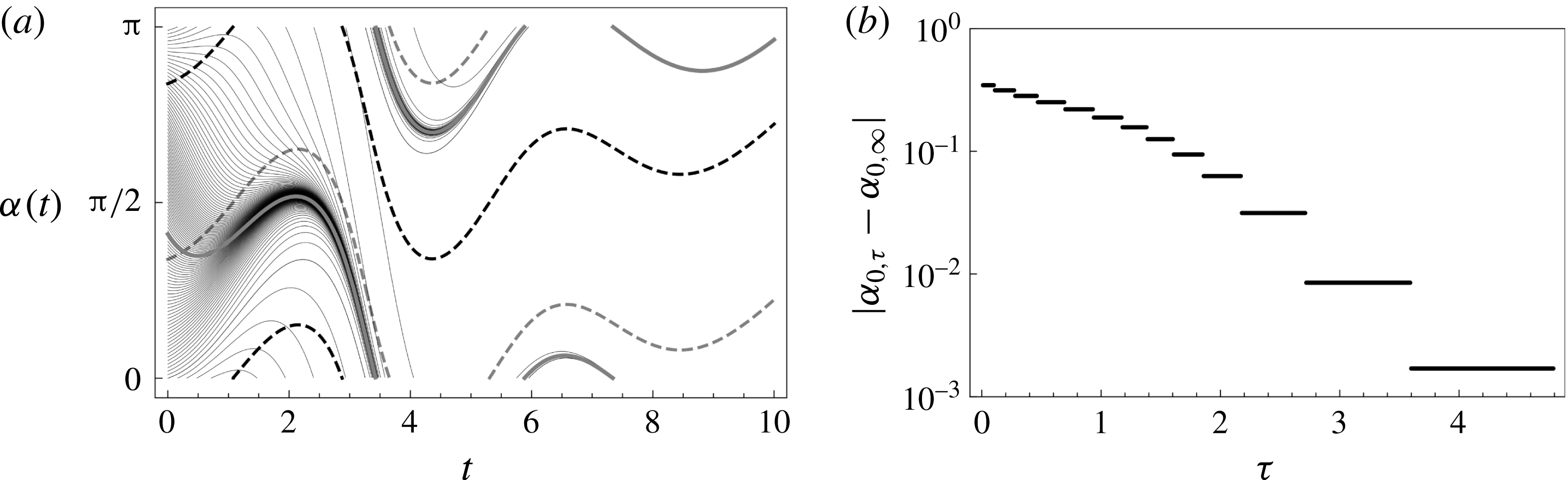
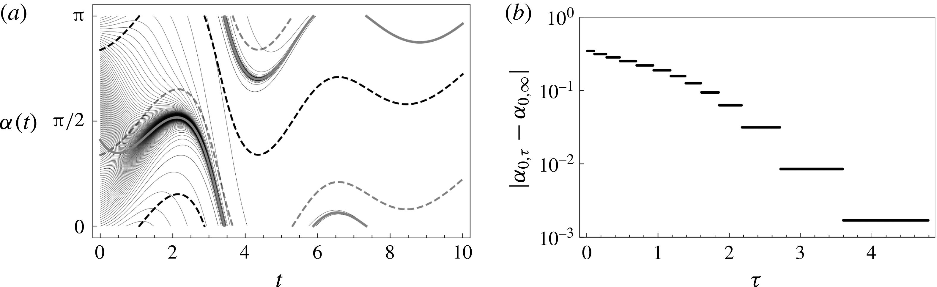
(a) Convergence of the transverse orientation angle
 $\unicode[STIX]{x1D6FC}(t)$
for different initial conditions
 $\unicode[STIX]{x1D6FC}(0)=\unicode[STIX]{x1D6FC}_{0}$
(thin black lines) toward the attracting trajectory
 ${\mathcal{M}}(t)=\unicode[STIX]{x1D6FC}(t;\unicode[STIX]{x1D6FC}_{0,\infty })$
(thick grey line) for the ABC flow. Note the correspondence between
 ${\mathcal{M}}(t)$
and the transverse angle
 $\unicode[STIX]{x1D6FC}(t)$
associated with minimum (grey dashed line) divergence
 $\unicode[STIX]{x2202}g/\unicode[STIX]{x2202}\unicode[STIX]{x1D6FC}(\unicode[STIX]{x1D6FC},t)$
responsible for creation of the attracting trajectory. The maximum divergence is also shown (black dashed line). (b) Convergence of the initial angle associated with the approximate attracting trajectory
 $\unicode[STIX]{x1D6FC}_{0,\unicode[STIX]{x1D70F}}$
toward the infinite-time limit
 $\unicode[STIX]{x1D6FC}_{0,\infty }$
.
Whilst the ODE (3.29) may be satisfied for any arbitrary initial condition
 $\unicode[STIX]{x1D6FC}(0)=\unicode[STIX]{x1D6FC}_{0}$
, resulting in non-uniqueness of
 $\unicode[STIX]{x1D750}^{\prime }(t)$
, this non-autonomous ODE is locally dissipative as reflected by the divergence
 $$\begin{eqnarray}\frac{\unicode[STIX]{x2202}g}{\unicode[STIX]{x2202}\unicode[STIX]{x1D6FC}}=[b(t)-a(t)]\sin 2\unicode[STIX]{x1D6FC}+c(t)\cos 2\unicode[STIX]{x1D6FC},\end{eqnarray}$$
which admits maxima and minima of magnitude
 $\pm c(t)\sqrt{1+[b(t)-a(t)/c(t)]^{2}}$
respectively at
 $$\begin{eqnarray}\unicode[STIX]{x1D6FC}(t)=\frac{1}{2}\arctan \left[\frac{b(t)-a(t)}{c(t)}\right]+\frac{\unicode[STIX]{x03C0}}{2}\frac{\text{sgn}\,c(t)\mp 1}{2}.\end{eqnarray}$$
Hence for
 $c(t)\neq 0$
, the ODE (3.29) admits an attracting trajectory
 ${\mathcal{M}}(t)$
, which attracts solutions from all initial conditions
 $\unicode[STIX]{x1D6FC}_{0}$
as illustrated in figure 2(a). As this trajectory is also a solution of (3.29), it may be expressed as
 ${\mathcal{M}}(t)=\unicode[STIX]{x1D6FC}(t;\unicode[STIX]{x1D6FC}_{0,\infty })$
, where
 $\unicode[STIX]{x1D6FC}_{0,\infty }$
is the initial condition at
 $t=0$
which is already on
 ${\mathcal{M}}(t)$
. Whilst all solutions of (3.29) render
 $\unicode[STIX]{x1D750}^{\prime }(t)$
upper triangular, only solutions along the attracting trajectory
 ${\mathcal{M}}(t)$
represent asymptotic dynamics independent of the initial condition
 $\unicode[STIX]{x1D6FC}_{0}$
, hence we define the Protean frame as that which corresponds to
 ${\mathcal{M}}(t)=\unicode[STIX]{x1D6FC}(t;\unicode[STIX]{x1D6FC}_{0,\infty })$
.
As the attracting trajectory
 ${\mathcal{M}}(t)$
maximises dissipation
 $-\unicode[STIX]{x2202}g/\unicode[STIX]{x2202}\unicode[STIX]{x1D6FC}$
over long times, the associated initial condition
 $\unicode[STIX]{x1D6FC}_{0,\infty }$
is quantified by the limit
 $\unicode[STIX]{x1D6FC}_{0,\infty }=\lim _{\unicode[STIX]{x1D70F}\rightarrow \infty }\unicode[STIX]{x1D6FC}_{0,\unicode[STIX]{x1D70F}}$
, where
 $$\begin{eqnarray}\unicode[STIX]{x1D6FC}_{0,\unicode[STIX]{x1D70F}}(t)=\arg \min _{\unicode[STIX]{x1D6FC}_{0}}\int _{0}^{\unicode[STIX]{x1D70F}}\frac{\unicode[STIX]{x2202}g(\unicode[STIX]{x1D6FC}(t^{\prime };\unicode[STIX]{x1D6FC}_{0}),t^{\prime })}{\unicode[STIX]{x2202}\unicode[STIX]{x1D6FC}}\,\text{d}t^{\prime }.\end{eqnarray}$$
Whilst
 ${\mathcal{M}}(t)$
can be identified by evolving (3.29) until acceptable convergence is obtained,
 ${\mathcal{M}}(t)$
may be identified at shorter times
 $\unicode[STIX]{x1D70F}\sim 1/|c|$
via the approximation (3.35), as shown in figure 2(b). This approach is particularly useful when Lagrangian data are only available over short times and explicitly identifies the inertial initial orientation angle
 $\unicode[STIX]{x1D6FC}_{0,\infty }$
, allowing the Protean transform to be determined uniquely from
 $t=0$
.
3.2.2 Longitudinal and transverse deformation in 3-D steady flow
Given solution of (3.29) (such that
 $\unicode[STIX]{x1D608}_{23}=\tilde{\unicode[STIX]{x1D716}}_{32}$
), reorientation into the Protean frame renders the streamline velocity gradient tensor
 $\unicode[STIX]{x1D750}^{\prime }(t)$
upper triangular. From (3.7) it follows that
 $\unicode[STIX]{x1D641}^{\prime }(t)$
is also upper triangular, with diagonal components
 $$\begin{eqnarray}\displaystyle & \displaystyle \unicode[STIX]{x1D60D}_{11}^{\prime }(t)=\frac{v(t)}{v(0)}, & \displaystyle\end{eqnarray}$$
 $$\begin{eqnarray}\displaystyle & \displaystyle \unicode[STIX]{x1D60D}_{ii}^{\prime }(t)=\exp \left[\int _{0}^{t}\text{d}t^{\prime }\unicode[STIX]{x1D716}_{ii}^{\prime }(t^{\prime })\right], & \displaystyle\end{eqnarray}$$
for
 $i=2,3$
. The off-diagonal elements are
 $\unicode[STIX]{x1D60D}_{ij}(t)=0$
for
 $i>j$
and else
 $$\begin{eqnarray}\displaystyle & \displaystyle \unicode[STIX]{x1D60D}_{12}^{\prime }(t)=v(t)\int _{0}^{t}\text{d}t^{\prime }\frac{\unicode[STIX]{x1D716}_{12}^{\prime }(t^{\prime })\unicode[STIX]{x1D60D}_{22}^{\prime }(t^{\prime })}{v(t^{\prime })}, & \displaystyle\end{eqnarray}$$
 $$\begin{eqnarray}\displaystyle & \displaystyle \unicode[STIX]{x1D60D}_{23}^{\prime }(t)=\unicode[STIX]{x1D60D}_{22}^{\prime }(t)\int _{0}^{t}\text{d}t^{\prime }\frac{\unicode[STIX]{x1D716}_{23}^{\prime }(t^{\prime })\unicode[STIX]{x1D60D}_{33}^{\prime }(t^{\prime })}{\unicode[STIX]{x1D60D}_{22}^{\prime }(t^{\prime })}, & \displaystyle\end{eqnarray}$$
 $$\begin{eqnarray}\displaystyle & \displaystyle \unicode[STIX]{x1D60D}_{13}^{\prime }(t)=v(t)\int _{0}^{t}\text{d}t^{\prime }\frac{\unicode[STIX]{x1D716}_{12}^{\prime }(t^{\prime })\unicode[STIX]{x1D60D}_{23}^{\prime }(t^{\prime })+\unicode[STIX]{x1D716}_{13}^{\prime }(t^{\prime })\unicode[STIX]{x1D60D}_{33}^{\prime }(t^{\prime })}{v(t^{\prime })}. & \displaystyle\end{eqnarray}$$
Here the upper triangular form of
 $\unicode[STIX]{x1D750}^{\prime }(t)$
simplifies solution of the deformation tensor
 $\unicode[STIX]{x1D641}^{\prime }(t)$
such that the integrals (3.36) can be solved sequentially, rather than the coupled ODE (3.4). It is interesting to note that the integrands of the shear deformations
 $\unicode[STIX]{x1D60D}_{12}^{\prime }(t)$
and
 $\unicode[STIX]{x1D60D}_{13}^{\prime }(t)$
are weighted by the inverse velocity. This implies that episodes of low velocity lead to an enhancement of shear-induced deformation; see also the discussion in Dentz et al. (Reference Dentz, Lester, Borgne and de Barros2016b
) for 2-D steady random flows. The impact of intermittent shear events in low velocity zones can be quantified using a stochastic deformation model based on continuous time random walks, as outlined in the next section. For compactness of notation we henceforth omit these primes, with the understanding that all quantities are in the Protean frame unless specified otherwise.
To illustrate how the deformation tensor controls longitudinal and transverse stretching of fluid elements, we decompose
 $\unicode[STIX]{x1D641}$
into longitudinal and transverse components respectively as
 $\unicode[STIX]{x1D641}(t)=\unicode[STIX]{x1D641}_{l}+\unicode[STIX]{x1D641}_{t}$
, where
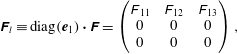 $$\begin{eqnarray}\displaystyle & \displaystyle \unicode[STIX]{x1D641}_{l}\equiv \text{diag}(\boldsymbol{e}_{1})\boldsymbol{\cdot }\unicode[STIX]{x1D641}=\left(\begin{array}{@{}ccc@{}}\unicode[STIX]{x1D60D}_{11} & \unicode[STIX]{x1D60D}_{12} & \unicode[STIX]{x1D60D}_{13}\\ 0 & 0 & 0\\ 0 & 0 & 0\\ \end{array}\right), & \displaystyle\end{eqnarray}$$
 $$\begin{eqnarray}\displaystyle & \displaystyle \unicode[STIX]{x1D641}_{t}\equiv \text{diag}(\boldsymbol{e}_{2}+\boldsymbol{e}_{3})\boldsymbol{\cdot }\unicode[STIX]{x1D641}=\left(\begin{array}{@{}ccc@{}}0 & 0 & 0\\ 0 & \unicode[STIX]{x1D60D}_{22} & \unicode[STIX]{x1D60D}_{23}\\ 0 & 0 & \unicode[STIX]{x1D60D}_{33}\end{array}\right), & \displaystyle\end{eqnarray}$$
where
 $\text{diag}(\boldsymbol{a})$
is a diagonal matrix comprising the vector
 $\boldsymbol{a}$
along the diagonal. From (3.2), a differential fluid line element
 $\unicode[STIX]{x1D6FF}\boldsymbol{l}(\boldsymbol{X},t)$
at Lagrangian position
 $\boldsymbol{X}$
then evolves with time
 $t$
as
 $$\begin{eqnarray}\displaystyle \unicode[STIX]{x1D6FF}\boldsymbol{l}(\boldsymbol{X},t) & = & \displaystyle \unicode[STIX]{x1D641}(\boldsymbol{X},t)\boldsymbol{\cdot }\unicode[STIX]{x1D6FF}\boldsymbol{l}(\boldsymbol{X},0)\nonumber\\ \displaystyle & = & \displaystyle \unicode[STIX]{x1D641}_{l}(\boldsymbol{X},t)\boldsymbol{\cdot }\unicode[STIX]{x1D6FF}\boldsymbol{l}(\boldsymbol{X},0)+\unicode[STIX]{x1D641}_{t}(\boldsymbol{X},t)\boldsymbol{\cdot }\unicode[STIX]{x1D6FF}\boldsymbol{l}(\boldsymbol{X},0)=\unicode[STIX]{x1D6FF}\boldsymbol{l}_{l}(\boldsymbol{X},t)+\unicode[STIX]{x1D6FF}\boldsymbol{l}_{t}(\boldsymbol{X},t),\end{eqnarray}$$
where the line element may also be decomposed into the longitudinal and transverse components as
 $\unicode[STIX]{x1D6FF}\boldsymbol{l}_{l}=\unicode[STIX]{x1D6FF}\boldsymbol{l}_{l}+\unicode[STIX]{x1D6FF}\boldsymbol{l}_{t}$
. Due to the upper triangular nature of
 $\unicode[STIX]{x1D641}$
the length
 $\unicode[STIX]{x1D6FF}l$
of these line elements can also be decomposed as
 $$\begin{eqnarray}\displaystyle \unicode[STIX]{x1D6FF}l(\boldsymbol{X},t)\equiv |\unicode[STIX]{x1D6FF}\boldsymbol{l}(\boldsymbol{X},t)| & = & \displaystyle \sqrt{\unicode[STIX]{x1D6FF}\boldsymbol{l}(\boldsymbol{X},0)\boldsymbol{\cdot }\unicode[STIX]{x1D641}^{\top }(\boldsymbol{X},t)\boldsymbol{\cdot }\unicode[STIX]{x1D641}(\boldsymbol{X},t)\boldsymbol{\cdot }\unicode[STIX]{x1D6FF}\boldsymbol{l}(\boldsymbol{X},0)}\nonumber\\ \displaystyle & = & \displaystyle \sqrt{\unicode[STIX]{x1D6FF}\boldsymbol{l}(\boldsymbol{X},0)\boldsymbol{\cdot }(\unicode[STIX]{x1D641}_{l}^{\top }(\boldsymbol{X},t)\boldsymbol{\cdot }\unicode[STIX]{x1D641}_{l}(\boldsymbol{X},t)+\unicode[STIX]{x1D641}_{t}^{\top }(\boldsymbol{X},t)\boldsymbol{\cdot }\unicode[STIX]{x1D641}_{t}(\boldsymbol{X},t))\boldsymbol{\cdot }\unicode[STIX]{x1D6FF}\boldsymbol{l}(\boldsymbol{X},0)}\nonumber\\ \displaystyle & = & \displaystyle \sqrt{\unicode[STIX]{x1D6FF}l_{l}(\boldsymbol{X},t)^{2}+\unicode[STIX]{x1D6FF}l_{t}(\boldsymbol{X},t)^{2}}.\end{eqnarray}$$
Hence the total length of the line element is decomposed into longitudinal and transverse contributions as
 $$\begin{eqnarray}\unicode[STIX]{x1D6FF}l^{2}=\unicode[STIX]{x1D6FF}l_{l}^{2}+\unicode[STIX]{x1D6FF}l_{t}^{2}.\end{eqnarray}$$
We denote the length of the 1-D lines
 ${\mathcal{H}}_{1\text{D}}^{(2)}$
,
 ${\mathcal{H}}_{1\text{D}}^{(3)}$
in figure 1 respectively as
 $l^{(2)}(t)$
,
 $l^{(3)}(\bar{x}_{1})$
, where the respective arguments
 $t$
,
 $\bar{x}_{1}$
reflect the fact that the 1-D line
 ${\mathcal{H}}_{1\text{D}}^{(2)}$
occurs at fixed time
 $t$
since injection, whereas the 1-D line
 ${\mathcal{H}}_{1\text{D}}^{(3)}$
occurs at fixed distance
 $\bar{x}_{1}$
downstream in the mean flow direction. Following the decomposition (3.41),
 $l^{(2)}(t)$
and
 $l^{(3)}(\bar{x}_{1})$
are then given by the contour integrals along the injection line
 ${\mathcal{H}}_{1\text{D}}^{(1)}$
in Lagrangian space as
 $$\begin{eqnarray}\displaystyle & \displaystyle l^{(2)}(t)=\int _{{\mathcal{H}}_{1\text{D}}^{(1)}}\sqrt{\unicode[STIX]{x1D6FF}l_{l}(\boldsymbol{X},t)^{2}+\unicode[STIX]{x1D6FF}l_{t}(\boldsymbol{X},t)^{2}}\,\text{d}s, & \displaystyle\end{eqnarray}$$
 $$\begin{eqnarray}\displaystyle & \displaystyle l^{(3)}(\bar{x}_{1})=\int _{{\mathcal{H}}_{1\text{D}}^{(1)}}\unicode[STIX]{x1D6FF}l_{l}(\boldsymbol{X},t_{1}(\boldsymbol{X},\bar{x}_{1}))\,\text{d}s, & \displaystyle\end{eqnarray}$$
where
 $\bar{t}_{1}(\boldsymbol{X},\bar{x}_{1})$
is the time at which the fluid streamline at Lagrangian coordinate
 $\boldsymbol{X}$
reaches
 $\bar{x}_{1}$
, and
 $\text{d}s$
is a differential increment associated with changes in
 $\boldsymbol{X}$
along
 ${\mathcal{H}}_{1\text{D}}^{(1)}$
. Hence stretching of the 1-D material line
 ${\mathcal{H}}_{1\text{D}}^{(2)}$
in figure 1 is governed by both the transverse and longitudinal deformations
 $\unicode[STIX]{x1D641}_{l}$
,
 $\unicode[STIX]{x1D641}_{t}$
, whereas stretching of the 1-D line
 ${\mathcal{H}}_{1\text{D}}^{(2)}$
transverse to the mean flow direction is solely governed by the transverse deformation
 $\unicode[STIX]{x1D641}_{t}$
.
As discussed in § 1, the deformation of these different lines is important for various applications. For example, Le Borgne et al. (Reference Le Borgne, Dentz and Villermaux2013, Reference Le Borgne, Dentz and Villermaux2015) use the growth rate of
 $l^{(2)}(t)$
to predict the mixing of a pulsed tracer injection (illustrated as
 ${\mathcal{H}}_{1\text{D}}^{(2)}$
in figure 1) in a steady 2-D Darcy flow. Conversely, Lester et al. (Reference Lester, Dentz and Le Borgne2016) use the growth rate of
 $l^{(3)}(t)$
to predict mixing of a continuously injected source in steady 3-D pore-scale flow. These different deformation rates indicate that a single scalar cannot be used to characterise fluid deformation in steady random 3-D flow. Instead it is necessary to characterise both longitudinal and transverse fluid deformation in such flows.
As such, we characterise longitudinal
 $\unicode[STIX]{x1D6EC}_{l}(t)$
and transverse
 $\unicode[STIX]{x1D6EC}_{t}(t)$
fluid deformation in terms of the corresponding deformation tensors as
 $$\begin{eqnarray}\displaystyle & \displaystyle \unicode[STIX]{x1D6EC}_{l}(t)\equiv \langle \Vert \unicode[STIX]{x1D641}_{l}(t)\Vert \rangle =\langle \sqrt{\unicode[STIX]{x1D60D}_{11}(t)^{2}+\unicode[STIX]{x1D60D}_{12}(t)^{2}+\unicode[STIX]{x1D60D}_{13}(t)^{2}}\rangle , & \displaystyle\end{eqnarray}$$
 $$\begin{eqnarray}\displaystyle & \displaystyle \unicode[STIX]{x1D6EC}_{t}(t)\equiv \langle \Vert \unicode[STIX]{x1D641}_{t}(t)\Vert \rangle =\langle \sqrt{\unicode[STIX]{x1D60D}_{22}(t)^{2}+\unicode[STIX]{x1D60D}_{23}(t)^{2}+\unicode[STIX]{x1D60D}_{33}(t)^{2}}\rangle , & \displaystyle\end{eqnarray}$$
where the angled brackets denote an ensemble average over multiple realisations of a 3-D steady random flow. We also define the ensemble-averaged length of an arbitrary fluid line as
 $$\begin{eqnarray}\ell (t)\equiv \langle \unicode[STIX]{x1D6FF}l(\boldsymbol{X},t)\rangle ,\end{eqnarray}$$
and in § 4, we seek to derive stochastic models for the growth of
 $\unicode[STIX]{x1D6EC}_{l}(t)$
,
 $\unicode[STIX]{x1D6EC}_{t}(t)$
and
 $\ell (t)$
in steady random 3-D flows. In 2-D steady flow, topological constraints (associated with conservation of area) prevent persistent growth of transverse deformation which simply fluctuates as
 $\unicode[STIX]{x1D6EC}_{t}(t)=\langle \unicode[STIX]{x1D60D}_{22}(t)\rangle =1/\langle \unicode[STIX]{x1D60D}_{11}(t)\rangle =\langle v(0)/v(t)\rangle =1$
. Conversely, longitudinal deformation can grow persistently as
 $\unicode[STIX]{x1D6EC}_{l}(t)\sim \unicode[STIX]{x1D60D}_{12}(t)^{2}$
, and Dentz et al. (Reference Dentz, Lester, Borgne and de Barros2016b
) derive stochastic models for the evolution of
 $\unicode[STIX]{x1D6EC}_{l}(t)$
from velocity field statistical properties as a CTRW. In § 4 we extend this approach to steady random 3-D flows to yield stochastic models for
 $\unicode[STIX]{x1D6EC}_{l}(t)$
,
 $\unicode[STIX]{x1D6EC}_{t}(t)$
and
 $\ell (t)$
, which act as important inputs for models of fluid mixing and dispersion.
For illustration, we briefly consider the deformation along the axis of the streamline coordinate system. For a fluid element
 $\boldsymbol{z}(t)$
initially aligned with the
 $1$
-direction of the Protean coordinate system, i.e.
 $\boldsymbol{z}(0)=(z_{0},0,0)^{\top }$
we obtain the elongation
 $\ell (t)=\sqrt{\boldsymbol{z}(t)^{2}}$
 $$\begin{eqnarray}\ell (t)=z_{0}\frac{v(t)}{v(0)}.\end{eqnarray}$$
For ergodic flows (i.e. where any streamline eventually samples all of the flow structure), the average stretching is zero and elongation will tend asymptotically toward a constant. For a material element initially orientated along the
 $2$
-direction of the Protean coordinate system, i.e.
 $\boldsymbol{z}(0)=(0,z_{0},0)^{\top }$
, we obtain the elongation
 $$\begin{eqnarray}\ell (t)=z_{0}\sqrt{\unicode[STIX]{x1D60D}_{12}(t)^{2}+\unicode[STIX]{x1D60D}_{22}(t)^{2}}.\end{eqnarray}$$
For an initial alignment with the
 $3$
-direction,
 $\boldsymbol{z}(0)=(0,0,z_{0})^{\top }$
 $$\begin{eqnarray}\ell (t)=z_{0}\sqrt{\unicode[STIX]{x1D60D}_{13}(t)^{2}+\unicode[STIX]{x1D60D}_{23}(t)^{2}+\unicode[STIX]{x1D60D}_{33}(t)^{2}}.\end{eqnarray}$$
In general, we have
 $$\begin{eqnarray}\ell (t)=\sqrt{\boldsymbol{z}_{0}\unicode[STIX]{x1D641}^{\top }(t)\unicode[STIX]{x1D641}(t)\boldsymbol{z}_{0}},\end{eqnarray}$$
where
 $\boldsymbol{z}(t=0)\equiv \boldsymbol{z}_{0}$
. Thus, net elongation is only achieved for initial orientations away from the velocity tangent. For both chaotic and non-chaotic flows, the explicit structure of
 $\unicode[STIX]{x1D641}^{\prime }(t)$
facilitates the identification of the stochastic dynamics of fluid deformation in steady random flows and its quantification in terms of the fluid velocity and velocity gradient statistics.
3.3 Zero-helicity-density flows
One important class of steady
 $D=3$
dimensional flows are zero helicity density (or complex lamellar (Finnigan Reference Finnigan1983)) flows such as the isotropic Darcy flow (Sposito Reference Sposito2001)
 $$\begin{eqnarray}\boldsymbol{v}(\boldsymbol{x})=-k(\boldsymbol{x})\unicode[STIX]{x1D735}\unicode[STIX]{x1D719}(\boldsymbol{x}),\end{eqnarray}$$
which is commonly used to model Darcy-scale flow in heterogeneous porous media. Here
 $\boldsymbol{v}(\boldsymbol{x})$
is the specific discharge, the scalar
 $k(\boldsymbol{x})$
represents hydraulic conductivity and
 $\unicode[STIX]{x1D719}(\boldsymbol{x})$
is the flow potential (or velocity head). For such flows the helicity density (Moffatt Reference Moffatt1969) which measures the helical motion of the flow,
 $$\begin{eqnarray}h(\boldsymbol{x})\equiv \boldsymbol{v}\boldsymbol{\cdot }\unicode[STIX]{x1D74E}=k(\boldsymbol{x})\unicode[STIX]{x1D735}\unicode[STIX]{x1D719}(\boldsymbol{x})\boldsymbol{\cdot }(\unicode[STIX]{x1D735}k(\boldsymbol{x})\times \unicode[STIX]{x1D735}\unicode[STIX]{x1D719}(\boldsymbol{x})),\end{eqnarray}$$
is identically zero (where
 $\unicode[STIX]{x1D74E}$
is the vorticity vector). As shown by Kelvin (Reference Kelvin1884), all 3-D zero-helicity-density flows are complex lamellar, and so may be posed in the form of an isotropic Darcy flow
 $\boldsymbol{v}(\boldsymbol{x})=-k(\boldsymbol{x})\unicode[STIX]{x1D735}\unicode[STIX]{x1D719}$
, where for porous media flow
 $\unicode[STIX]{x1D719}$
is the flow potential and
 $k(\boldsymbol{x})$
represents the (possibly heterogeneous) hydraulic conductivity. Arnol’d (Reference Arnol’d1965, Reference Arnol’d1966) shows that streamlines in complex lamellar steady zero-helicity-density flows are confined to a set of two orthogonal
 $D=2$
dimensional integral surfaces which can be interpreted as level sets of two stream functions
 $\unicode[STIX]{x1D713}_{1}$
,
 $\unicode[STIX]{x1D713}_{2}$
, with
 $\unicode[STIX]{x1D735}\unicode[STIX]{x1D713}_{1}\boldsymbol{\cdot }\unicode[STIX]{x1D735}\unicode[STIX]{x1D713}_{2}=0$
. As such, all zero helicity density flows may be represented as
 $$\begin{eqnarray}\boldsymbol{v}(\boldsymbol{x})=-k(\boldsymbol{x})\unicode[STIX]{x1D735}\unicode[STIX]{x1D719}=\unicode[STIX]{x1D735}\unicode[STIX]{x1D713}_{1}\times \unicode[STIX]{x1D735}\unicode[STIX]{x1D713}_{2}.\end{eqnarray}$$
As the gradients
 $\unicode[STIX]{x1D735}\unicode[STIX]{x1D719}$
,
 $\unicode[STIX]{x1D735}\unicode[STIX]{x1D713}_{1}$
,
 $\unicode[STIX]{x1D735}\unicode[STIX]{x1D713}_{2}$
are all mutually orthogonal, zero-helicity-density flows admit an orthogonal streamline coordinate system (
 $\unicode[STIX]{x1D719}$
,
 $\unicode[STIX]{x1D713}_{1}$
,
 $\unicode[STIX]{x1D713}_{2}$
) with unit base vectors
 $$\begin{eqnarray}\hat{\boldsymbol{e}}_{1}=-\frac{\unicode[STIX]{x1D735}\unicode[STIX]{x1D719}}{\Vert \unicode[STIX]{x1D735}\unicode[STIX]{x1D719}\Vert }=\frac{\boldsymbol{v}}{\Vert \boldsymbol{v}\Vert },\quad \hat{\boldsymbol{e}}_{2}=\frac{\unicode[STIX]{x1D735}\unicode[STIX]{x1D713}_{1}}{\Vert \unicode[STIX]{x1D735}\unicode[STIX]{x1D713}_{1}\Vert },\quad \hat{\boldsymbol{e}}_{3}=\frac{\unicode[STIX]{x1D735}\unicode[STIX]{x1D713}_{2}}{\Vert \unicode[STIX]{x1D735}\unicode[STIX]{x1D713}_{2}\Vert }.\end{eqnarray}$$
If the streamfunctions
 $\unicode[STIX]{x1D713}_{1}$
,
 $\unicode[STIX]{x1D713}_{2}$
are known, there is no need to explicitly solve the orientation angle
 $\unicode[STIX]{x1D6FC}(t)$
via (3.29), but rather the Protean frame can be determined from the coordinate directions given by (3.54). Note that the moving Protean coordinate frame differs from an orthogonal curvilinear streamline coordinate system based on (3.54), and we show in appendix B that such a coordinate system does not yield an upper triangular velocity gradient.
The zero-helicity-density condition imposes important constraints upon the Lagrangian kinematics of these flows. First, as steady zero helicity-density flows must be non-chaotic due to integrability of the streamsurfaces
 $\unicode[STIX]{x1D713}_{1}$
,
 $\unicode[STIX]{x1D713}_{2}$
(Holm & Kimura Reference Holm and Kimura1991), hence fluid deformation must be sub-exponential (algebraic). From (3.36b
), the ensemble average of the principal components
 $\unicode[STIX]{x1D716}_{ii}$
of the velocity gradient deformation (which correspond to the Lyapunov exponents of the flow) must be zero. Secondly, zero-helicity flows constrain the velocity gradient components such that
 $\tilde{\unicode[STIX]{x1D716}}_{23}=\tilde{\unicode[STIX]{x1D716}}_{32}$
, due to the identity
 $$\begin{eqnarray}h=\boldsymbol{v}\boldsymbol{\cdot }\unicode[STIX]{x1D74E}=\boldsymbol{v}\boldsymbol{\cdot }(\unicode[STIX]{x1D700}_{ijk}:\unicode[STIX]{x1D750})=\tilde{\boldsymbol{v}}\boldsymbol{\cdot }(\unicode[STIX]{x1D700}_{ijk}:\tilde{\unicode[STIX]{x1D750}})=v(\tilde{\unicode[STIX]{x1D716}}_{23}-\tilde{\unicode[STIX]{x1D716}}_{32})=0,\end{eqnarray}$$
where
 $\unicode[STIX]{x1D700}_{ijk}$
is the Levi-Civita tensor. Whilst (3.55) shows
 $\tilde{\unicode[STIX]{x1D716}}_{23}=\tilde{\unicode[STIX]{x1D716}}_{32}$
in general for zero helicity flows, there exists a specific value of
 $\unicode[STIX]{x1D6FC}$
, denoted
 $\tilde{\unicode[STIX]{x1D6FC}}$
, which renders both
 $\tilde{\unicode[STIX]{x1D716}}_{23}$
and
 $\tilde{\unicode[STIX]{x1D716}}_{32}$
zero. This form of the velocity gradient (namely zero (2,3) and (3,2) components) is reflected by its representation in the curvilinear streamline coordinate system shown in appendix B, and can lead to a decoupling of fluid deformation between the (1,2) and (1,3) planes. However, as the Protean frame is a moving coordinate system, there is a non-zero contribution from
 $\unicode[STIX]{x1D63C}(t)$
to the (2,3) and (3,2) components of the velocity gradient. Typically, a different value of
 $\unicode[STIX]{x1D6FC}$
is used than
 $\tilde{\unicode[STIX]{x1D6FC}}$
to render
 $\unicode[STIX]{x1D716}_{32}^{\prime }=0$
, and so for zero helicity flow
 $$\begin{eqnarray}\unicode[STIX]{x1D716}_{23}^{\prime }=2\tilde{\unicode[STIX]{x1D716}}_{23},\end{eqnarray}$$
which is typically non-zero, hence
 $\unicode[STIX]{x1D60D}_{23}^{\prime }\neq 0$
in general. Note that as both the Protean coordinate frame and the curvilinear streamline coordinate system render the deformation tensor component
 $\unicode[STIX]{x1D60D}_{23}$
non-zero (see appendix B for details), the coupling between fluid deformation in the (1,2) and (1,3) planes is retained in both coordinate frames, hence this is not purely an artefact of the moving coordinate system.
The confinement of streamlines to integral streamsurfaces given by the level sets of
 $\unicode[STIX]{x1D713}_{1}$
,
 $\unicode[STIX]{x1D713}_{2}$
effectively means that steady 3-D zero-helicity-density flows can be considered as two superposed steady
 $D=2$
dimensional flows. This has several impacts upon the transport and deformation dynamics. First, as the 2-D integral surfaces are topological cylinders or tori, streamlines confined within these surfaces cannot diverge exponentially in space. Thus, the principal transverse deformations
 $\unicode[STIX]{x1D60D}_{22}$
,
 $\unicode[STIX]{x1D60D}_{33}$
in the Protean frame may only fluctuate about the unit mean as
 $$\begin{eqnarray}\langle \unicode[STIX]{x1D60D}_{ii}\rangle =1,\quad i=1,2,3,\end{eqnarray}$$
and so the only persistent growth of fluid deformation in steady zero helicity flows only occurs via the longitudinal and transverse shear deformations
 $\unicode[STIX]{x1D60D}_{12}$
,
 $\unicode[STIX]{x1D60D}_{13}$
,
 $\unicode[STIX]{x1D60D}_{23}$
. Secondly, as the streamlines of this steady flow are confined to 2-D integral surfaces, exponential fluid stretching (such as occurs in chaotic advection) is not possible due to constraints associated with the Poincaré–Bendixson theorem. Hence the shear deformations may only grow algebraically in time, i.e.
 $$\begin{eqnarray}\displaystyle & \displaystyle \lim _{t\rightarrow \infty }\langle \unicode[STIX]{x1D60D}_{12}(s)\rangle \sim t^{r_{12}}, & \displaystyle\end{eqnarray}$$
 $$\begin{eqnarray}\displaystyle & \displaystyle \lim _{t\rightarrow \infty }\langle \unicode[STIX]{x1D60D}_{13}(s)\rangle \sim t^{r_{13}}, & \displaystyle\end{eqnarray}$$
 $$\begin{eqnarray}\displaystyle & \displaystyle \lim _{t\rightarrow \infty }\langle \unicode[STIX]{x1D60D}_{23}(s)\rangle \sim t^{r_{23}}. & \displaystyle\end{eqnarray}$$
Dentz et al. (Reference Dentz, Lester, Borgne and de Barros2016b
) develop a CTRW model for shear deformation in steady random incompressible 2-D flows and uncover algebraic stretching of
 $\unicode[STIX]{x1D60D}_{12}\sim t^{r}$
(again in Protean coordinates) and show that the index
 $r$
depends upon the coupling between shear deformation and velocity fluctuations long streamlines, ranging from diffusive
 $r=1/2$
to superdiffusive
 $r=2$
stretching.
Hence fluid deformation is constrained to be algebraic in steady 3-D zero-helicity-density flow, and evolves in a similar fashion to steady 2-D flow,
 $$\begin{eqnarray}\displaystyle & \displaystyle \unicode[STIX]{x1D6EC}_{t}(t)\sim t^{r_{23}}, & \displaystyle\end{eqnarray}$$
 $$\begin{eqnarray}\displaystyle & \displaystyle \unicode[STIX]{x1D6EC}_{l}(t)\sim t^{max(r_{12},r_{13})}, & \displaystyle\end{eqnarray}$$
where the indices
 $r$
are governed by intermittency of the fluid shear events (Dentz et al.
Reference Dentz, Lester, Borgne and de Barros2016b
). We note that these constraints do not apply to anisotropic Darcy flows (i.e.
 $\boldsymbol{v}(\boldsymbol{x})=-\boldsymbol{K}(\boldsymbol{x})\boldsymbol{\cdot }\unicode[STIX]{x1D735}\unicode[STIX]{x1D719}(\boldsymbol{x})$
, where
 $\boldsymbol{K}(\boldsymbol{x})$
is the tensorial hydraulic conductivity), as these no longer correspond to zero-helicity-density flows. Indeed, as demonstrated by Ye et al. (Reference Ye, Chiogna, Cirpka, Grathwohl and Rolle2015), these flows can give rise to chaotic advection and exponential stretching of material elements. We consider fluid deformation in such steady chaotic flows in the following section.
3.3.1 Fluid deformation along stagnation lines
For streamlines which connect with a stagnation point (termed stagnation lines), the solution of the deformation tensor (3.36) diverges in the neighbourhood of the stagnation point as
 $v\rightarrow 0$
. To circumvent this issue, we consider fluid deformation along a stagnation line in the neighbourhood of a stagnation point
 $\boldsymbol{x}_{p}$
, where the velocity gradient may be approximated as
 $\unicode[STIX]{x1D750}(t)\approx \unicode[STIX]{x1D750}_{0}\equiv \unicode[STIX]{x1D750}|_{\boldsymbol{x}=\boldsymbol{x}_{p}}$
. Note that for streamlines approaching a stagnation point from upstream,
 $\unicode[STIX]{x1D716}_{11,0}$
must necessarily be negative. In the neighbourhood of the stagnation point, the velocity evolves as
 $v(t)/v(t_{0})\approx \exp (\unicode[STIX]{x1D716}_{11,0}(t-t_{0}))$
, and the deformation gradient tensor can be solved directly from (3.4) as
 $$\begin{eqnarray}\unicode[STIX]{x1D641}(t)\approx \unicode[STIX]{x1D641}(t_{0})\boldsymbol{\cdot }\exp (\unicode[STIX]{x1D750}_{0}(t-t_{0})),\end{eqnarray}$$
where
 $t_{0}$
is the time at which the fluid element enters the neighbourhood of the stagnation point (defined as the region for which
 $\unicode[STIX]{x1D750}(t)\approx \unicode[STIX]{x1D750}_{0}$
). Note that (3.36) represents an explicit solution of the matrix exponential above, via the substitutions
 $t\mapsto t-t_{0}$
,
 $v(t)\mapsto v(t_{0})\exp (\unicode[STIX]{x1D716}_{11,0}(t-t_{0}))$
,
 $\unicode[STIX]{x1D750}(t)\mapsto \unicode[STIX]{x1D750}_{0}$
. Whilst the stochastic model for fluid deformation developed herein does apply to points of zero fluid velocity, the impact of deformation local to stagnation points can be included a posteriori via (3.63).
4 Stochastic fluid deformation in steady random 3-D flow
In this section, we develop a stochastic model for fluid deformation along streamlines in steady
 $D=3$
dimensional flows that exhibit chaotic advection and exponential fluid stretching. This model is based on a continuous-time random walk (CTRW) framework for particle transport in steady random flows, which is briefly summarised in the following.
4.1 Continous-time random walks for fluid velocities
The travel distance
 $s(t)$
of a fluid particle along a streamline is given by
 $$\begin{eqnarray}\frac{\text{d}s(t)}{\text{d}t}=v_{s}[s(t)],\quad \frac{\text{d}t(s)}{\text{d}s}=\frac{1}{v_{s}(s)},\end{eqnarray}$$
where
 $v_{s}(s)=v[t(s)]$
. We note that fluid velocities
 $v_{s}(s)$
can be represented as a Markov process that evolves with distance along fluid streamlines (Dentz et al.
Reference Dentz, Kang, Comolli, Le Borgne and Lester2016a
) for flow through heterogeneous porous and fractured media from pore to Darcy and regional scales (Berkowitz et al.
Reference Berkowitz, Cortis, Dentz and Scher2006; Fiori et al.
Reference Fiori, Jankovic, Dagan and Cvetkovic2007; Le Borgne et al.
Reference Le Borgne, Dentz and Carrera2008a
,Reference Le Borgne, Dentz and Carrera
b
; Bijeljic, Mostaghimi & Blunt Reference Bijeljic, Mostaghimi and Blunt2011; De Anna et al.
Reference De Anna, Le Borgne, Dentz, Tartakovsky, Bolster and Davy2013; Holzner et al.
Reference Holzner, Morales, Willmann and Dentz2015; Kang et al.
Reference Kang, Dentz, Le Borgne and Juanes2015). This property stems from the fact that fluid velocities evolve on characteristic spatial scales imprinted in the spatial flow structure. Streamwise velocities
 $v_{s}(s)$
are correlated on the correlation scale
 $\ell _{c}$
. For distances larger than
 $\ell _{c}$
subsequent particle velocities can be considered independent. Thus, particle motion along streamlines can be represented by the recursion relations
 $$\begin{eqnarray}s_{n+1}=s_{n}+\ell _{c},\quad t_{n+1}=t_{n}+\frac{\ell _{c}}{v_{n}},\end{eqnarray}$$
where we defined
 $v_{n}=v(s_{n})$
for the
 $n$
th step. The position
 $s(t)$
along a streamline is given in terms of (4.2) by
 $s(t)=s_{n_{t}}$
, where
 $n_{t}=\sup (n|t_{n}\leqslant t)$
, the particle speed is given by
 $v(t)=n_{n_{t}}$
. This coarse-grained picture is valid for times larger than the advection time scale
 $\unicode[STIX]{x1D70F}_{u}=\ell _{c}/\overline{u}$
, where
 $\overline{u}$
is the mean flow velocity. We consider flow fields that are characterised by open ergodic streamlines. Thus,
 $v_{n}$
can be modelled as independent identically distributed random variables that are characterised by
 $p_{s}(v)$
. The latter is related to the probability density function (PDF)
 $p_{e}(v)$
of Eulerian velocities
 $v_{e}$
through flux weighting as (Dentz et al.
Reference Dentz, Kang, Comolli, Le Borgne and Lester2016a
)
 $$\begin{eqnarray}p_{s}(v)=\frac{vp_{e}(v)}{\langle v_{e}\rangle }.\end{eqnarray}$$
The advective transition time over the characteristic distance
 $\ell _{c}$
is defined by
 $$\begin{eqnarray}\unicode[STIX]{x1D70F}_{n}=\frac{\ell _{c}}{v_{n}}.\end{eqnarray}$$
Its distribution
 $\unicode[STIX]{x1D713}(t)$
is obtained from (4.3) in terms of the Eulerian PDF
 $p_{e}(v)$
as
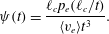 $$\begin{eqnarray}\unicode[STIX]{x1D713}(t)=\frac{\ell _{c}p_{e}(\ell _{c}/t)}{\langle v_{e}\rangle t^{3}}.\end{eqnarray}$$
Equations (4.2) constitute a continuous-time random walk (CTRW) in that the time increment
 $\unicode[STIX]{x1D70F}_{n}\equiv \ell _{c}/v_{n}$
at the
 $n$
th random walk step is a continuous random variable, unlike for discrete time random walks, which describe Markov processes in time. The CTRW is also called a semi-Markovian framework because the governing equations (4.2) are Markovian in step number, while any Markovian process
 $A_{n}$
when projected on time as
 $A(t)=A_{n_{t}}$
is non-Markovian.
In order to illustrate this notion, we consider the joint evolution of a process
 $A_{n}$
and time
 $t_{n}$
along a streamline (Scher & Lax Reference Scher and Lax1973),
 $$\begin{eqnarray}A_{n+1}=A_{n}+\unicode[STIX]{x0394}A_{n},\quad t_{n+1}=t_{n}+\unicode[STIX]{x1D70F}_{n}.\end{eqnarray}$$
The increments
 $(\unicode[STIX]{x0394}A,\unicode[STIX]{x1D70F})$
are stepwise independent and in general coupled. They are characterised by the joint PDF
 $\unicode[STIX]{x1D713}_{a}(a,t)$
, which can be written as
 $$\begin{eqnarray}\unicode[STIX]{x1D713}_{a}(a,t)=\unicode[STIX]{x1D713}_{a}(a|t)\unicode[STIX]{x1D713}(t),\end{eqnarray}$$
The PDF
 $p_{a}(a,t)$
of
 $A(t)$
is then given by
 $$\begin{eqnarray}p_{a}(a,t)=\int _{0}^{t}\text{d}t^{\prime }R(a,t^{\prime })\int _{t-t^{\prime }}^{\infty }\text{d}t^{\prime \prime }\unicode[STIX]{x1D713}(t),\end{eqnarray}$$
where
 $R(a,t)$
denotes the probability per time that
 $A(t)$
has just assumed the value
 $a$
. Thus, equation (4.8) can be read as follows. The probability
 $p_{a}(a,t)$
that
 $A(t)$
has the value
 $a$
at time
 $t$
is equal to the probability per time
 $R(a,t^{\prime })$
that
 $A(t)$
has arrived at
 $a$
times the probability that the next transition takes longer than
 $t-t^{\prime }$
. The
 $R(a,t)$
satisfies the Chapman–Kolmogorov-type equation
 $$\begin{eqnarray}R(a,t)=R_{0}(a,t)+\int _{0}^{t}\text{d}t^{\prime }\int \text{d}a\unicode[STIX]{x1D713}(a-a^{\prime },t-t^{\prime })R(a^{\prime },t^{\prime }),\end{eqnarray}$$
where
 $R_{0}(a,t)$
is the joint distribution of
 $A_{0}$
and
 $t_{0}$
. Equations (4.8) and (4.9) can be combined into the following generalised master equation (Kenkre, Montroll & Shlesinger Reference Kenkre, Montroll and Shlesinger1973) for the evolution of
 $p_{a}(t)$
:
 $$\begin{eqnarray}\frac{\unicode[STIX]{x2202}p_{a}(a,t)}{\unicode[STIX]{x2202}t}=\int _{0}^{t}\text{d}t^{\prime }\int \text{d}a\unicode[STIX]{x1D6F7}(a-a^{\prime },t-t^{\prime })[p_{a}(a^{\prime },t^{\prime })-p_{a}(a,t^{\prime })],\end{eqnarray}$$
where
 $\unicode[STIX]{x1D6F7}(a,t)$
is defined in Laplace space as
 $$\begin{eqnarray}\unicode[STIX]{x1D6F7}^{\ast }(a,\unicode[STIX]{x1D706})=\frac{\unicode[STIX]{x1D706}\unicode[STIX]{x1D713}_{a}^{\ast }(a,\unicode[STIX]{x1D706})}{1-\unicode[STIX]{x1D713}^{\ast }(\unicode[STIX]{x1D706})}.\end{eqnarray}$$
The general master equation (4.10) expresses the non-Markovian character of the evolution of the statistics of
 $A(t)$
.
In the following, we develop a stochastic model for deformation based on these relations. We anticipate that the velocity gradient statistics also follow a spatial Markov process with similar correlation structure. Spatial Markovianity of both the fluid velocity and velocity gradient then provides a basis for stochastic modelling of the deformation equations (3.36b,e ) as a coupled continuous-time random walk (coupled CTRW) along streamlines, in a similar fashion to that developed by Dentz et al. (Reference Dentz, Lester, Borgne and de Barros2016b ) for deformation in steady 2-D random flow. Based on the explicit expressions (3.36) of the deformation tensor, this stochastic approach is derived from first principles and so provides a link to Lagrangian velocity and deformation, which in turn may be linked to the Eulerian flow properties and medium characteristics (Fiori et al. Reference Fiori, Jankovic, Dagan and Cvetkovic2007; Edery et al. Reference Edery, Guadagnini, Scher and Berkowitz2014; Dentz et al. Reference Dentz, Kang, Comolli, Le Borgne and Lester2016a ; Tyukhova et al. Reference Tyukhova, Dentz, Kinzelbach and Willmann2016).
To this end, we recast (3.36) in terms of the distance along the streamline by using the transformation (4.1) from
 $t$
to
 $s$
. This gives for the diagonal components of
 $\hat{\unicode[STIX]{x1D641}}(s)=\unicode[STIX]{x1D641}[t(s)]$
 $$\begin{eqnarray}\displaystyle & \displaystyle \hat{\unicode[STIX]{x1D60D}}_{11}(s)=\frac{v_{s}(s)}{v_{s}(0)}, & \displaystyle\end{eqnarray}$$
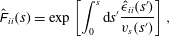 $$\begin{eqnarray}\displaystyle & \displaystyle \hat{\unicode[STIX]{x1D60D}}_{ii}(s)=\exp \left[\int _{0}^{s}\text{d}s^{\prime }\frac{\hat{\unicode[STIX]{x1D716}}_{ii}(s^{\prime })}{v_{s}(s^{\prime })}\right], & \displaystyle\end{eqnarray}$$
with
 $i=2,3$
. For the off-diagonal elements, we obtain
 $$\begin{eqnarray}\displaystyle & \displaystyle \hat{\unicode[STIX]{x1D60D}}_{12}(s)=v_{s}(s)\int _{0}^{s}\text{d}s^{\prime }\frac{\hat{\unicode[STIX]{x1D716}}_{12}(s^{\prime })\hat{\unicode[STIX]{x1D60D}}_{22}(s^{\prime })}{v_{s}(s^{\prime })^{2}}, & \displaystyle\end{eqnarray}$$
 $$\begin{eqnarray}\displaystyle & \displaystyle \hat{\unicode[STIX]{x1D60D}}_{23}(s)=\hat{\unicode[STIX]{x1D60D}}_{22}(s)\int _{0}^{s}\text{d}s^{\prime }\frac{\hat{\unicode[STIX]{x1D716}}_{23}(s^{\prime })\hat{\unicode[STIX]{x1D60D}}_{33}(s^{\prime })}{v_{s}(s^{\prime })\unicode[STIX]{x1D60D}_{22}(s^{\prime })}, & \displaystyle\end{eqnarray}$$
 $$\begin{eqnarray}\displaystyle & \displaystyle \hat{\unicode[STIX]{x1D60D}}_{13}(s)=v_{s}(s)\int _{0}^{s}\text{d}s^{\prime }\frac{\hat{\unicode[STIX]{x1D716}}_{12}(s^{\prime })\hat{\unicode[STIX]{x1D60D}}_{23}(s^{\prime })+\hat{\unicode[STIX]{x1D716}}_{13}(s^{\prime })\hat{\unicode[STIX]{x1D60D}}_{33}(s^{\prime })}{v_{s}(s^{\prime })^{2}}, & \displaystyle\end{eqnarray}$$
while
 $\hat{\unicode[STIX]{x1D60D}}_{ij}(s)=0$
for
 $i>j$
. We denote
 $\hat{\unicode[STIX]{x1D716}}_{ij}(s)=\unicode[STIX]{x1D716}_{ij}[t(s)]$
. In the following, we investigate the evolution of stretching in different time regimes for chaotic steady random flow.
4.2 Chaotic steady random flow
For chaotic flows, the infinite-time Lyapunov exponent is defined by
 $$\begin{eqnarray}\unicode[STIX]{x1D706}\equiv \lim _{t\rightarrow \infty }\lim _{z_{0}\rightarrow 0}\frac{1}{2t}\ln \left[\frac{\ell (t)^{2}}{\ell (0)^{2}}\right].\end{eqnarray}$$
In the limit of
 $t\gg \unicode[STIX]{x1D706}^{-1}$
, we may set
 $$\begin{eqnarray}\unicode[STIX]{x1D60D}_{11}(t)=1,\quad \unicode[STIX]{x1D60D}_{22}(t)=\exp (\unicode[STIX]{x1D716}t),\quad \unicode[STIX]{x1D60D}_{33}(t)=\exp (-\unicode[STIX]{x1D716}t),\end{eqnarray}$$
where we defined
 $$\begin{eqnarray}\unicode[STIX]{x1D716}=\lim _{t\rightarrow \infty }\frac{1}{t}\int _{0}^{t}\text{d}t^{\prime }\unicode[STIX]{x1D716}_{22}(t^{\prime })=-\!\lim _{t\rightarrow \infty }\frac{1}{t}\int _{0}^{t}\text{d}t^{\prime }\unicode[STIX]{x1D716}_{33}(t^{\prime }).\end{eqnarray}$$
The last equation is due to volume conservation. The long-time behaviour is fully dominated by exponential stretching. The characteristic stretching time scale for exponential stretching is given by
 $\unicode[STIX]{x1D70F}_{\unicode[STIX]{x1D716}}=1/\unicode[STIX]{x1D716}$
, while the characteristic advection scale is
 $\unicode[STIX]{x1D70F}_{u}=\ell _{c}/\overline{u}$
with
 $\overline{u}$
the mean and
 $\ell _{c}$
the correlation scale of the steady random flow field
 $\boldsymbol{u}(\boldsymbol{x})$
. The latter sets the end of the ballistic regimes: see below. If
 $\unicode[STIX]{x1D70F}_{\unicode[STIX]{x1D716}}$
and
 $\unicode[STIX]{x1D70F}_{u}$
are well separated,
 $\unicode[STIX]{x1D70F}_{\unicode[STIX]{x1D716}}\gg \unicode[STIX]{x1D70F}_{u}$
, we observe a subexponential stretching regime that is dominated by heterogeneous shear action. In the following, we analyse the behaviour of deformation for time
 $t\ll \unicode[STIX]{x1D70F}_{\unicode[STIX]{x1D716}}$
. We first briefly discuss the ballistic regime for which
 $t\ll \unicode[STIX]{x1D70F}_{u}$
. Then, we develop a CTRW based approach for deformation in the pre-exponential regime
 $\unicode[STIX]{x1D70F}_{u}\ll t\ll \unicode[STIX]{x1D70F}_{\unicode[STIX]{x1D716}}$
.
4.2.1 Ballistic regime:
$t\ll \unicode[STIX]{x1D70F}_{u}$

We first consider the ballistic short-time regime, for which
 $t\ll \unicode[STIX]{x1D70F}_{u}$
. In this regime, the flow properties are essentially constant and we obtain the approximation for the deformation tensor (3.36),
 $$\begin{eqnarray}\unicode[STIX]{x1D60D}_{ii}(t)=1,\end{eqnarray}$$
for
 $i=1,2,3$
and for the off-diagonal elements with
 $i>j$
,
 $$\begin{eqnarray}\unicode[STIX]{x1D60D}_{12}(t)=\unicode[STIX]{x1D716}_{12}t,\quad \unicode[STIX]{x1D60D}_{23}(t)=\unicode[STIX]{x1D716}_{23}t,\quad \unicode[STIX]{x1D60D}_{13}(t)=(\unicode[STIX]{x1D716}_{12}\unicode[STIX]{x1D716}_{23}t/2+\unicode[STIX]{x1D716}_{13})t.\end{eqnarray}$$
As
 $\unicode[STIX]{x1D716}_{ij}\sim 1/\unicode[STIX]{x1D70F}_{u}$
, in this regime the transverse (3.45) and longitudinal (3.44) deformations as well as the arbitrary fluid element
 $\ell (t)$
all evolve ballistically to leading order:
 $\unicode[STIX]{x1D6EC}_{t}(t)$
,
 $\unicode[STIX]{x1D6EC}_{l}(t)$
,
 $\ell (t)\propto t$
.
4.2.2 Exponential stretching regime
$t\gg \unicode[STIX]{x1D70F}_{\unicode[STIX]{x1D716}}$

In the stretching regime, for times much larger than
 $\unicode[STIX]{x1D70F}_{\unicode[STIX]{x1D716}}$
, the principal deformations scale as
 $$\begin{eqnarray}\unicode[STIX]{x1D60D}_{11}(t)=1,\quad \unicode[STIX]{x1D60D}_{22}(t)=\exp (\unicode[STIX]{x1D716}t),\quad \unicode[STIX]{x1D60D}_{33}(t)=\exp (-\unicode[STIX]{x1D716}t).\end{eqnarray}$$
In this regime the expressions for the off-diagonal elements of
 $\unicode[STIX]{x1D641}(t)$
in (3.36) can be approximated by
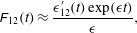 $$\begin{eqnarray}\displaystyle & \displaystyle \unicode[STIX]{x1D60D}_{12}(t)\approx \frac{\unicode[STIX]{x1D716}_{12}^{\prime }(t)\exp (\unicode[STIX]{x1D716}t)}{\unicode[STIX]{x1D716}}, & \displaystyle\end{eqnarray}$$
 $$\begin{eqnarray}\displaystyle & \displaystyle \unicode[STIX]{x1D60D}_{23}(t)\approx \exp (\unicode[STIX]{x1D716}t)\int _{0}^{t}\text{d}t^{\prime }\unicode[STIX]{x1D716}_{23}^{\prime }(t^{\prime })\exp (-2\unicode[STIX]{x1D716}t^{\prime }), & \displaystyle\end{eqnarray}$$
 $$\begin{eqnarray}\displaystyle & \displaystyle \unicode[STIX]{x1D60D}_{13}(t)\approx \unicode[STIX]{x1D60D}_{12}(t)\unicode[STIX]{x1D716}_{12}(t)\int _{0}^{t}\text{d}t^{\prime }\unicode[STIX]{x1D716}_{23}^{\prime }(t^{\prime })\exp (-2\unicode[STIX]{x1D716}t^{\prime }). & \displaystyle\end{eqnarray}$$
Note that the integrals above are dominated through the exponential by the upper limit, which gives these approximations. In this regime the longitudinal (3.44) and transverse deformations (3.45), along with the elongation of a material element (3.50) all increase exponentially with time:
 $\unicode[STIX]{x1D6EC}_{l}(t)$
,
 $\unicode[STIX]{x1D6EC}_{t}(t)$
,
 $\ell (t)\propto \exp (\unicode[STIX]{x1D716}t)$
. From (4.13) the Lyapunov exponent is then
 $\unicode[STIX]{x1D706}\equiv \unicode[STIX]{x1D716}$
.
4.2.3 Intermediate regime
$t>\unicode[STIX]{x1D70F}_{u}$

For times
 $t>\unicode[STIX]{x1D70F}_{u}$
, we develop a CTRW approach to describe the impact of flow heterogeneity on the evolution of the deformation tensor, based on (4.2) and (4.12). In this regime, we approximate
 $\hat{\unicode[STIX]{x1D60D}}_{11}(s)\approx 1$
,
 $\hat{\unicode[STIX]{x1D60D}}_{22}(s)\approx \exp [\unicode[STIX]{x1D706}t(s)]$
and
 $\unicode[STIX]{x1D60D}_{33}\approx \exp [-\unicode[STIX]{x1D706}t(s)]$
. The off-diagonal components are then expressed as
 $$\begin{eqnarray}\displaystyle \hat{\unicode[STIX]{x1D60D}}_{12}(s)=\frac{v_{s}(s)}{\ell _{c}}r_{2}(s),\quad \hat{\unicode[STIX]{x1D60D}}_{23}(s)=\hat{\unicode[STIX]{x1D60D}}_{22}(s)p(s), & & \displaystyle\end{eqnarray}$$
 $$\begin{eqnarray}\displaystyle \hat{\unicode[STIX]{x1D60D}}_{13}(s)=v_{s}(s)\int _{0}^{s}\text{d}s^{\prime }\frac{\hat{\unicode[STIX]{x1D716}}_{12}(s^{\prime })\hat{\unicode[STIX]{x1D60D}}_{23}(s^{\prime })}{v_{s}(s^{\prime })^{2}}+\frac{v(s)}{\ell _{c}}r_{3}(s), & & \displaystyle\end{eqnarray}$$
where we defined the auxiliary functions
 $$\begin{eqnarray}\frac{\text{d}r_{i}(s)}{\text{d}s}=\ell _{c}\frac{\hat{\unicode[STIX]{x1D716}}_{1i}(s)\hat{\unicode[STIX]{x1D60D}}_{ii}(s)}{v_{s}(s)^{2}},\quad i=2,3,\quad \frac{\text{d}p(s)}{\text{d}s}=\frac{\hat{\unicode[STIX]{x1D716}}_{23}(s)\hat{\unicode[STIX]{x1D60D}}_{33}(s)}{v_{s}(s)\unicode[STIX]{x1D60D}_{22}(s)},\end{eqnarray}$$
with
 $r_{i}(s=0)=0$
and
 $p(s=0)=0$
. We approximated the off-diagonal components
 $\hat{\unicode[STIX]{x1D716}}_{ij}(s)$
for
 $i>j$
as being
 $\unicode[STIX]{x1D6FF}$
-correlated on the scales of interest such that
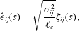 $$\begin{eqnarray}\hat{\unicode[STIX]{x1D716}}_{ij}(s)=\sqrt{\frac{\unicode[STIX]{x1D70E}_{ij}^{2}}{\ell _{c}}}\unicode[STIX]{x1D709}_{ij}(s),\end{eqnarray}$$
where
 $\unicode[STIX]{x1D709}(s)$
denotes white noise with zero mean and correlation
 $\langle \unicode[STIX]{x1D709}_{ij}(s)\unicode[STIX]{x1D709}_{ij}(s^{\prime })\rangle =\unicode[STIX]{x1D6FF}(s-s^{\prime })$
, and the
 $\unicode[STIX]{x1D70E}_{ij}$
are characteristic deformation rates. We assume here that the deformation rates are independent of velocity magnitude, an assumption that can be easily relaxed. Discretising (4.22) on the scale
 $\ell _{c}$
such that
 $s_{n}=n\ell _{c}$
and using (4.23), we obtain
 $$\begin{eqnarray}\displaystyle & \displaystyle r_{i,n+1}=r_{i,n}+\unicode[STIX]{x1D70F}_{n}^{2}\unicode[STIX]{x1D70E}_{1i}\exp [(-1)^{i}\unicode[STIX]{x1D706}t_{n}]\unicode[STIX]{x1D709}_{1i,n},\quad i=2,3, & \displaystyle\end{eqnarray}$$
 $$\begin{eqnarray}\displaystyle & \displaystyle p_{n+1}=p_{n}+\unicode[STIX]{x1D70F}_{n}\unicode[STIX]{x1D70E}_{23}\exp (-2\unicode[STIX]{x1D706}t_{n})\unicode[STIX]{x1D709}_{23,n}. & \displaystyle\end{eqnarray}$$
 $t_{n}$
. Note that
 $\unicode[STIX]{x1D60D}_{ij}(t)=\hat{\unicode[STIX]{x1D60D}}_{ij}[s_{n_{t}}]=\hat{\unicode[STIX]{x1D60D}}_{ij}(n_{t}\ell _{c})$
. Thus, from (4.24) we obtain for the mean square deformations
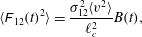 $$\begin{eqnarray}\displaystyle & \displaystyle \langle \unicode[STIX]{x1D60D}_{12}(t)^{2}\rangle =\frac{\unicode[STIX]{x1D70E}_{12}^{2}\langle v^{2}\rangle }{\ell _{c}^{2}}B(t), & \displaystyle\end{eqnarray}$$
 $$\begin{eqnarray}\displaystyle & \displaystyle \langle \unicode[STIX]{x1D60D}_{23}(t)^{2}\rangle =\frac{\unicode[STIX]{x1D70E}_{23}^{2}\langle \unicode[STIX]{x1D70F}^{2}\rangle }{4\unicode[STIX]{x1D706}}\exp (2\unicode[STIX]{x1D706}t)[1-\exp (-4\unicode[STIX]{x1D706}t)], & \displaystyle\end{eqnarray}$$
 $$\begin{eqnarray}\displaystyle & \displaystyle \langle \unicode[STIX]{x1D60D}_{13}(t)^{2}\rangle =\frac{\langle v^{2}\rangle \unicode[STIX]{x1D70E}_{12}^{2}\unicode[STIX]{x1D70E}_{23}^{2}\langle \unicode[STIX]{x1D70F}^{2}\rangle }{4\unicode[STIX]{x1D706}\ell _{c}^{2}}A(t)+\frac{\langle v^{2}\rangle \unicode[STIX]{x1D70E}_{13}^{2}}{\ell _{c}}B(t), & \displaystyle\end{eqnarray}$$
where we define
 $$\begin{eqnarray}\displaystyle & \displaystyle A(t)=\left\langle \mathop{\sum }_{i=0}^{n_{t}-1}\unicode[STIX]{x1D70F}_{i}^{4}\exp (2\unicode[STIX]{x1D706}\text{i}\langle \unicode[STIX]{x1D70F}\rangle )[1-\exp (-4\unicode[STIX]{x1D706}\text{i}\langle \unicode[STIX]{x1D70F}\rangle )]\right\rangle , & \displaystyle\end{eqnarray}$$
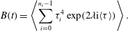 $$\begin{eqnarray}\displaystyle & \displaystyle B(t)=\left\langle \mathop{\sum }_{i=0}^{n_{t}-1}\unicode[STIX]{x1D70F}_{i}^{4}\exp (2\unicode[STIX]{x1D706}\text{i}\langle \unicode[STIX]{x1D70F}\rangle )\right\rangle . & \displaystyle\end{eqnarray}$$
In order to further develop these expressions, we consider heavy-tailed velocity distributions that behave as
 $$\begin{eqnarray}p_{s}(v)\propto v^{\unicode[STIX]{x1D6FD}-1},\end{eqnarray}$$
for
 $v<v_{0}$
with
 $v_{0}$
a characteristic velocity and
 $\unicode[STIX]{x1D6FD}>1$
. Such power-law type behaviour of the velocity PDF for small velocities is characteristic of observed transport behaviour in heterogeneous porous media (Berkowitz et al.
Reference Berkowitz, Cortis, Dentz and Scher2006). From (4.30), the transition time PDF behaves as
 $\unicode[STIX]{x1D713}(t)\propto t^{-1-\unicode[STIX]{x1D6FD}}$
for large
 $t$
. Note that the moments
 $\langle \unicode[STIX]{x1D70F}^{k}\rangle$
of
 $\unicode[STIX]{x1D713}(t)$
are finite for
 $k<\lfloor \unicode[STIX]{x1D6FD}\rfloor$
, where
 $\lfloor \cdot \rfloor$
denotes the floor function. For illustration, here we consider the case
 $\unicode[STIX]{x1D6FD}>2$
, which implies
 $\langle \unicode[STIX]{x1D70F}^{2}\rangle <\infty$
.
Shear-dominated regime
 $(\unicode[STIX]{x1D70F}_{u}\ll t\ll \unicode[STIX]{x1D70F}_{\unicode[STIX]{x1D716}})$
. We now determine the stretching behaviour in the shear-dominated time regime
 $\unicode[STIX]{x1D70F}_{u}\ll t\ll \unicode[STIX]{x1D70F}_{\unicode[STIX]{x1D716}}$
. In this time regime, we approximate (4.28) as
 $$\begin{eqnarray}A(t)=4\unicode[STIX]{x1D706}\left\langle \mathop{\sum }_{i=0}^{n_{t}-1}\text{i}\unicode[STIX]{x1D70F}_{i}^{4}\right\rangle ,\quad B(t)=\left\langle \mathop{\sum }_{i=0}^{n_{t}-1}\unicode[STIX]{x1D70F}_{i}^{4}\right\rangle .\end{eqnarray}$$
These expressions may be estimated as follows. We note that transitions that contribute to the elongation at time
 $t$
must have durations shorter than
 $t$
, i.e.
 $\unicode[STIX]{x1D70F}_{n}<t$
because
 $t_{n_{t}}=\sum _{i=0}^{n_{t}-1}\unicode[STIX]{x1D70F}_{i}<t$
. Thus, we can approximate
 $$\begin{eqnarray}A(t)\approx 4\unicode[STIX]{x1D706}\int _{0}^{t}\text{d}t^{\prime }{t^{\prime }}^{4}\unicode[STIX]{x1D713}(t^{\prime })\mathop{\sum }_{i=0}^{\langle n_{t}\rangle -1}\text{i}\propto t^{6-\unicode[STIX]{x1D6FD}},\end{eqnarray}$$
where we approximated
 $\langle n_{t}\rangle \approx t/\langle \unicode[STIX]{x1D70F}\rangle$
. Using the same approximations for
 $B(t)$
in (4.31) gives
 $B(t)\propto t^{5-\unicode[STIX]{x1D6FD}}$
. These scalings are consistent with the ones known for coupled continuous-time random walks (Dentz et al.
Reference Dentz, Le Borgne, Lester and de Barros2015). Hence, in the regime
 $\unicode[STIX]{x1D70F}_{u}\ll t\ll \unicode[STIX]{x1D70F}_{\unicode[STIX]{x1D716}}$
the transverse (3.45) deformation evolves linearly with time,
 $\langle \unicode[STIX]{x1D6EC}_{t}(t)^{2}\rangle \propto t$
, because
 $\unicode[STIX]{x1D60D}_{22}(t)$
and
 $\unicode[STIX]{x1D60D}_{33}(t)$
are approximately constant whilst
 $\langle \unicode[STIX]{x1D60D}_{23}(t)^{2}\rangle \propto t$
according to (4.26). The longitudinal (3.44) and material (3.50) deformations evolve nonlinearly to leading order as
 $\langle \unicode[STIX]{x1D6EC}_{l}(t)^{2}\rangle \propto \langle \ell (t)^{2}\rangle t^{6-\unicode[STIX]{x1D6FD}}$
according to (4.32).
Cross-over
 $(t\gtrsim \unicode[STIX]{x1D70F}_{\unicode[STIX]{x1D716}})$
. We now focus on the cross-over from the power-law to exponential stretching regimes. For
 $t\gtrsim \unicode[STIX]{x1D70F}_{\unicode[STIX]{x1D716}}$
, we approximate
 $A(t)\approx B(t)$
in (4.28) because the second term is exponentially small, and
 $B(t)$
is given by (4.29). Along the same lines as above, we derive for
 $B(t)$
 $$\begin{eqnarray}B(t)=\int _{0}^{t}\text{d}t^{\prime }{t^{\prime }}^{4}\unicode[STIX]{x1D713}(t^{\prime })\mathop{\sum }_{i=0}^{\langle n_{t}\rangle -1}\exp (2\unicode[STIX]{x1D706}\text{i}\langle \unicode[STIX]{x1D70F}\rangle )\propto t^{4-\unicode[STIX]{x1D6FD}}[\exp (2\unicode[STIX]{x1D706}t)-1].\end{eqnarray}$$
To test these expressions developed throughout this section, we simulate the non-stationary coupled CTRW (4.24) for
 $10^{5}$
fluid particles over 500 spatial steps over the range of Lyapunov exponents
 $\unicode[STIX]{x1D706}\in (10^{-1},10^{-2},10^{-3})$
. The velocity gradients
 $\hat{\unicode[STIX]{x1D716}}_{22}$
,
 $\hat{\unicode[STIX]{x1D716}}_{12}$
are modelled as Gaussian variables with mean
 $\unicode[STIX]{x1D706}$
and zero respectively, the mean travel time
 $\langle \unicode[STIX]{x1D70F}\rangle =10^{-1}$
, and the variances
 $\unicode[STIX]{x1D70E}_{22}^{2}=\unicode[STIX]{x1D70E}_{12}^{2}=1$
. Here the velocity PDF is given by the Nakagami distribution
 $$\begin{eqnarray}p_{v}(v;k,\unicode[STIX]{x1D703})=\frac{2}{\unicode[STIX]{x1D6E4}(k)}\left(\frac{k}{\unicode[STIX]{x1D703}}\right)^{k}v^{2k-1}\text{e}^{-kv^{2}/\unicode[STIX]{x1D703}},\quad v>0,\end{eqnarray}$$
with the parameters
 $k=1$
,
 $\unicode[STIX]{x1D703}=10$
. The PDFs of the velocities in the numerical test cases used in § 5 are very well characterised by this distribution. As such the PDF of
 $\unicode[STIX]{x1D70F}=\ell _{c}/v$
is then
 $$\begin{eqnarray}\unicode[STIX]{x1D713}(\unicode[STIX]{x1D70F})=\frac{\ell _{c}}{\unicode[STIX]{x1D70F}^{2}}p_{v}(\ell _{c}/\unicode[STIX]{x1D70F}),\end{eqnarray}$$
hence
 $\unicode[STIX]{x1D713}(t)\propto t^{-1-\unicode[STIX]{x1D6FD}}$
with
 $\unicode[STIX]{x1D6FD}=2k$
for
 $t>\unicode[STIX]{x1D70F}_{u}$
. The transition from algebraic to exponential growth is clearly shown in figure 3(b), where some deviation from the predicted exponential growth is observed for small
 $\unicode[STIX]{x1D6FD}$
due to the heavy-tailed nature of
 $\unicode[STIX]{x1D713}(\unicode[STIX]{x1D70F})$
.
Comparison between analytic predictions of
 $B(t)$
(4.29) for
 $t>\unicode[STIX]{x1D70F}_{u}$
(grey dashed) with numerical simulations from the synthetic coupled CTRW (4.24) (solid dark grey, solid blue online) for
 $\unicode[STIX]{x1D6FD}\in (1.5,2.5,3.5)$
(plots are offset for clarity with
 $\unicode[STIX]{x1D6FD}$
increasing from bottom to top) and (a)
 $\unicode[STIX]{x1D706}=10^{-3}$
,
 $\unicode[STIX]{x1D70E}_{22}=10^{-3}$
, (b)
 $\unicode[STIX]{x1D706}=10^{-2}$
,
 $\unicode[STIX]{x1D70E}_{22}=10^{-2}$
, (c)
 $\unicode[STIX]{x1D706}=10^{-1}$
,
 $\unicode[STIX]{x1D70E}_{22}=10^{-1}$
.
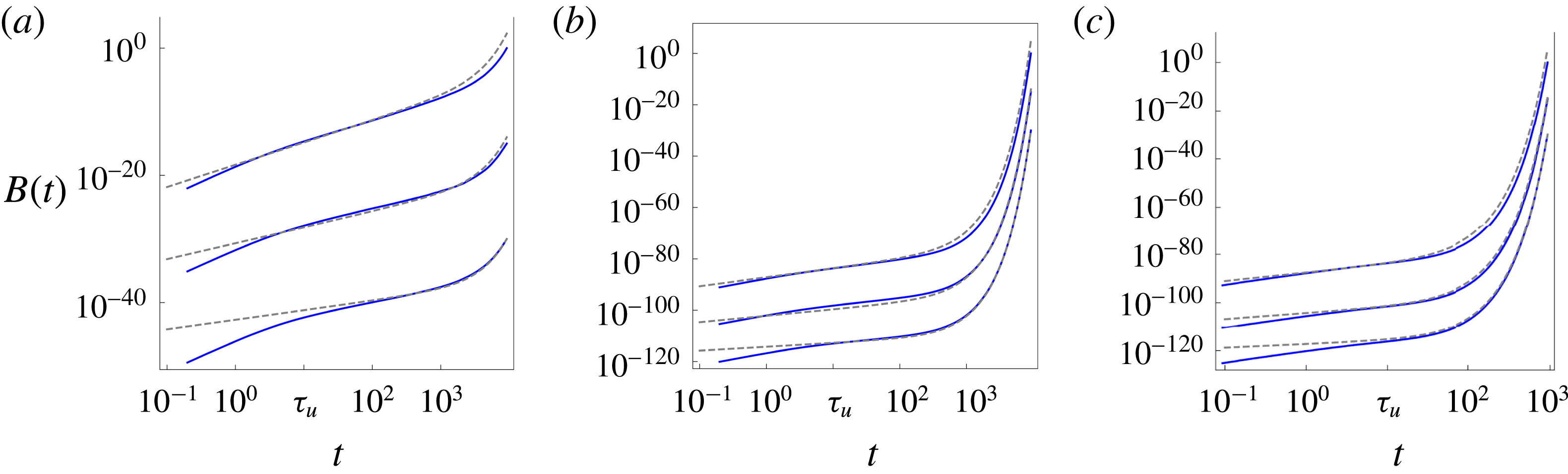
5 Fluid deformation in a model random 3-D flow
To study fluid deformation in flow where the stretching regimes described in §§ 4.2.1–4.2.3 overlap, we consider a steady incompressible random flow with variable exponential stretching, the variable-helicity (VH) flow. This flow is similar to that introduced by Dean, Drummond & Horgan (Reference Dean, Drummond and Horgan2001), which involves the helicity parameter
 $\unicode[STIX]{x1D713}\in [0,\unicode[STIX]{x03C0}/2]$
which controls the ensemble averaged helicity
 $\langle \boldsymbol{v}\boldsymbol{\cdot }\unicode[STIX]{x1D74E}\rangle$
of the random flow. The velocity field of the VH flow is given by
 $$\begin{eqnarray}\boldsymbol{v}(\boldsymbol{x};\unicode[STIX]{x1D713})=\mathop{\sum }_{n=1}^{N}[\unicode[STIX]{x1D74C}_{n}(\unicode[STIX]{x1D713})\times \boldsymbol{k}_{n}\cos (\boldsymbol{k}(\unicode[STIX]{x1D713})\boldsymbol{\cdot }(\boldsymbol{x}+\unicode[STIX]{x1D734}_{n}))+\unicode[STIX]{x1D74C}_{n}(\unicode[STIX]{x1D713})\times \boldsymbol{k}_{n}\sin (\boldsymbol{k}(\unicode[STIX]{x1D713})\boldsymbol{\cdot }(\boldsymbol{x}+\unicode[STIX]{x1D734}_{n}))],\end{eqnarray}$$
where the phase angle
 $\unicode[STIX]{x1D734}$
is a random vector with independent, uniformly distributed components in
 $[0,2\unicode[STIX]{x03C0}]$
, and
 $\unicode[STIX]{x1D74C}(\unicode[STIX]{x1D713})$
,
 $\boldsymbol{k}(\unicode[STIX]{x1D713})$
are the random vectors
 $$\begin{eqnarray}\displaystyle & \displaystyle \unicode[STIX]{x1D74C}(\unicode[STIX]{x1D713})=(\sin (\unicode[STIX]{x1D703}\sin \unicode[STIX]{x1D713})\sin \unicode[STIX]{x1D719},\sin (\unicode[STIX]{x1D703}\sin \unicode[STIX]{x1D713})\cos \unicode[STIX]{x1D719},\cos (\unicode[STIX]{x1D703}\sin \unicode[STIX]{x1D713})), & \displaystyle\end{eqnarray}$$
 $$\begin{eqnarray}\displaystyle & \displaystyle \boldsymbol{k}(\unicode[STIX]{x1D713})=(\sin (\unicode[STIX]{x1D703}\sin \unicode[STIX]{x1D713})\sin \unicode[STIX]{x1D719},\sin (\unicode[STIX]{x1D703}\sin \unicode[STIX]{x1D713})\cos \unicode[STIX]{x1D719},\cos (\unicode[STIX]{x1D703}\sin \unicode[STIX]{x1D713})), & \displaystyle\end{eqnarray}$$
where
 $\unicode[STIX]{x1D703}$
,
 $\unicode[STIX]{x1D719}$
are the independent, uniformly distributed variables
 $\unicode[STIX]{x1D703}\in [-\unicode[STIX]{x03C0}/2,\unicode[STIX]{x03C0}/2]$
,
 $\unicode[STIX]{x1D719}\in [-\unicode[STIX]{x03C0},\unicode[STIX]{x03C0}]$
. This flow is divergence-free, and converges to a multi-Gaussian field with sufficiently large
 $N$
; we use
 $N=64$
throughout. For
 $\unicode[STIX]{x1D713}=0$
, the VH flow is two-dimensional and constrained to the
 $x_{1}$
,
 $x_{2}$
plane, and for
 $\unicode[STIX]{x1D713}=\unicode[STIX]{x03C0}/2$
the flow is a fully 3-D flow. Hence fluid stretching increases monotonically from non-chaotic
 $\unicode[STIX]{x1D706}=0$
to globally chaotic
 $\unicode[STIX]{x1D706}\approx \ln 2$
over the range
 $\unicode[STIX]{x1D713}\in [0,\unicode[STIX]{x03C0}/2]$
. We consider fluid deformation for the two cases
 $\unicode[STIX]{x1D713}=\unicode[STIX]{x03C0}/64$
,
 $\unicode[STIX]{x1D713}=\unicode[STIX]{x03C0}/2$
, which corresponds to weak and strong exponential stretching respectively. Representative streamlines and velocity contours for both of these cases are shown in figure 4, which clearly illustrates the quasi-2-D and fully 3-D flow structures for
 $\unicode[STIX]{x1D713}=\unicode[STIX]{x03C0}/64$
,
 $\unicode[STIX]{x1D713}=\unicode[STIX]{x03C0}/2$
respectively.
We consider
 $10^{5}$
realisations of the VH flow for
 $\unicode[STIX]{x1D713}=\unicode[STIX]{x03C0}/2$
,
 $\unicode[STIX]{x1D713}=\unicode[STIX]{x03C0}/64$
, and for each realisation a particle trajectory is calculated over the time period
 $t\in [0,10^{2}]$
to precision
 $10^{-14}$
via an implicit Gauss–Legendre method. The associated deformation tensor in the Eulerian frame is calculated via solution of (3.4) to the same precision via the discrete QR decomposition method (due to the large associated deformations, in excess of
 $~10^{100}$
). The Protean velocity gradient tensor
 $\unicode[STIX]{x1D750}^{\prime }(t)$
is then computed along these trajectories by solution of the attracting trajectory
 ${\mathcal{M}}(t)$
(3.29) via an explicit Runge–Kutta method over a fixed time step (
 $\unicode[STIX]{x0394}t=10^{-3}$
) and the Protean deformation gradient tensor
 $\unicode[STIX]{x1D641}^{\prime }(t)$
is calculated by direct evaluation of the integrals (4.12). These results are compared with direct computation of the deformation tensor via (3.4) in the Cartesian frame, and the error between these methods is found to be of the same order as the integration precision.
Typical particle trajectory in a realisation of the variable helicity flow for (a)
 $\unicode[STIX]{x1D713}=\unicode[STIX]{x03C0}/2$
, (c)
 $\unicode[STIX]{x1D713}=\unicode[STIX]{x03C0}/64$
, and contour plot of velocity magnitude distribution in
 $x_{3}=0$
plane for (b)
 $\unicode[STIX]{x1D713}=\unicode[STIX]{x03C0}/2$
, (d)
 $\unicode[STIX]{x1D713}=\unicode[STIX]{x03C0}/64$
.
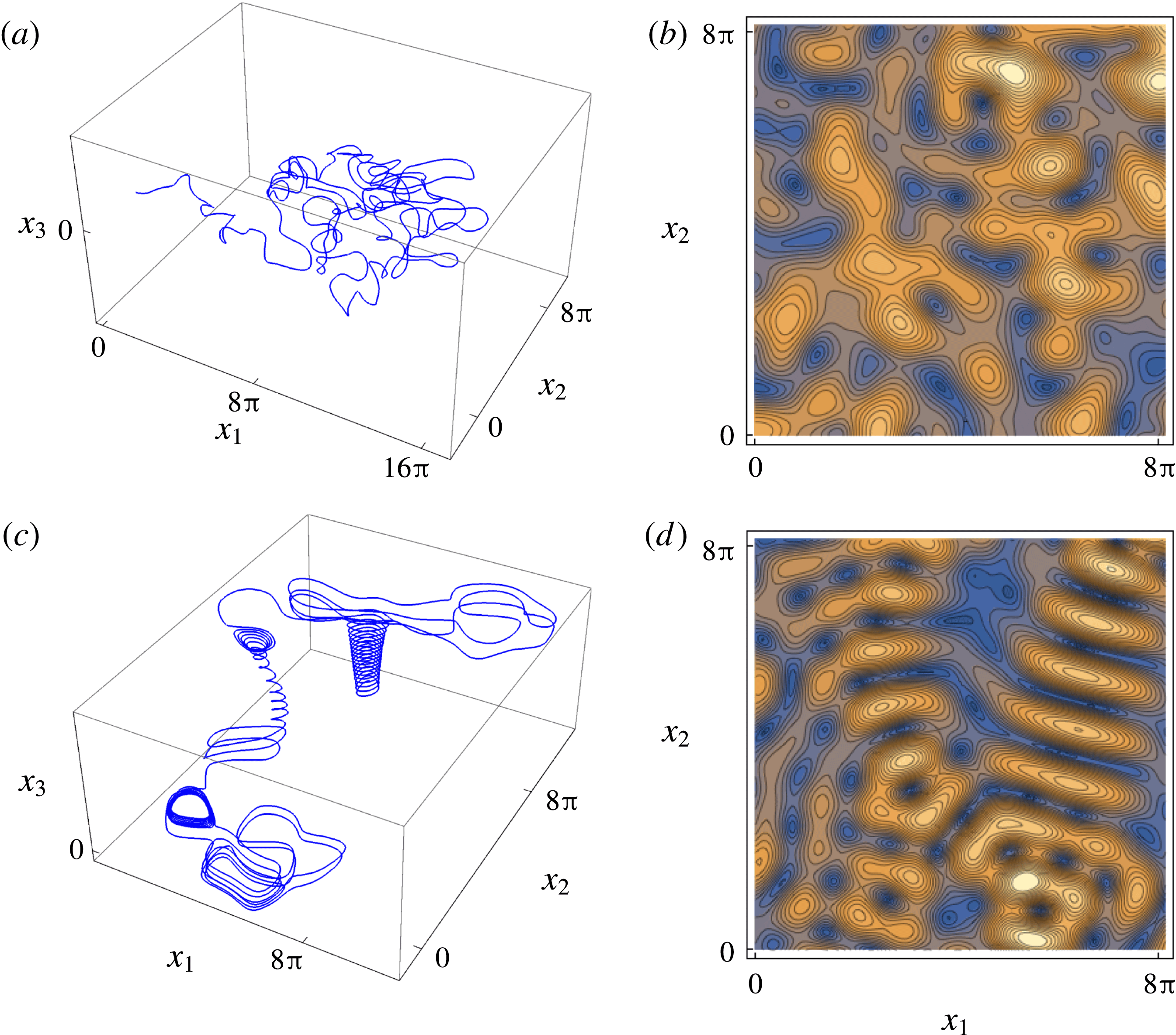
As shown in figure 5(a), the velocity
 $v(s)$
for both values of
 $\unicode[STIX]{x1D713}$
is well described by the Nakagami distribution (4.34), which exhibits power-law scaling
 $p_{v}(v)\sim v^{-1+2k}$
in the limit of small
 $v$
. The long waiting times associated with this power-law scaling has significant implications for anomalous transport and stretching dynamics, as will be shown. The autocorrelation structure of the velocity field along streamlines is shown in figure 5(b), indicating exponential decay which may be modelled as a first-order process for the correlation function
 $$\begin{eqnarray}R(s)=\langle v(s^{\prime })v(s^{\prime }-s)\rangle \approx \exp (-s/l_{c}),\end{eqnarray}$$
where the correlation length scale
 $\ell _{c}$
is estimated as
 $\ell _{c}=\int _{0}^{\infty }\text{d}sR(s)$
. This observation is consistent with the hypothesis used in (4.2) that steady random flows exhibit spatial Markovianity along streamlines (Le Borgne et al.
Reference Le Borgne, Dentz and Carrera2008a
,Reference Le Borgne, Dentz and Carrera
b
).
(a) Velocity probability distribution function (solid) with fitted Nakagami PDF (dashed), and (b) autocorrelation structure of fluid velocity
 $v(s)$
for the variable helical flow with
 $\unicode[STIX]{x1D713}=\unicode[STIX]{x03C0}/2$
(light) and
 $\unicode[STIX]{x1D713}=\unicode[STIX]{x03C0}/64$
(dark).
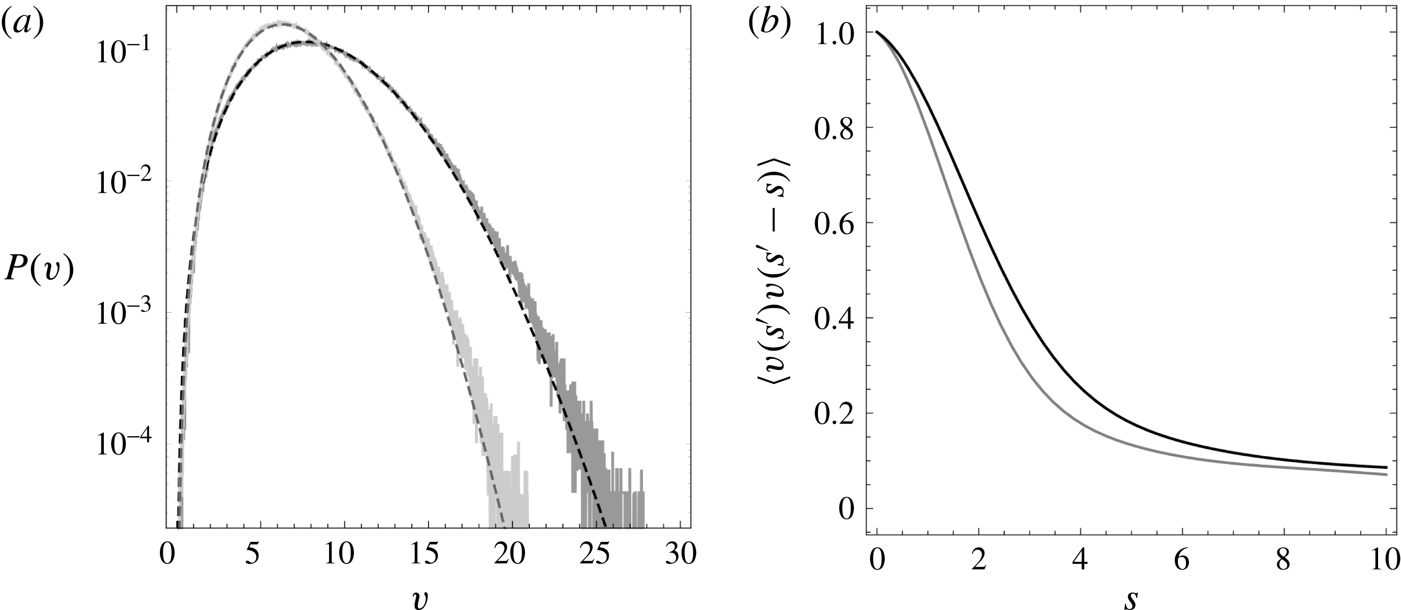
The distributions of the components of the velocity gradient tensor
 $\unicode[STIX]{x1D750}^{\prime }$
for both
 $\unicode[STIX]{x1D713}=\unicode[STIX]{x03C0}/2$
and
 $\unicode[STIX]{x1D713}=\unicode[STIX]{x03C0}/64$
are shown in figure 6, where for
 $\unicode[STIX]{x1D713}=\unicode[STIX]{x03C0}/2$
all of the components are Gaussian-distributed. The diagonal components have approximately the same variance
 $\unicode[STIX]{x1D70E}_{ij}^{2}\equiv \langle (\unicode[STIX]{x1D716}_{ij}^{\prime }-\langle \unicode[STIX]{x1D716}_{ij}^{\prime }\rangle )^{2}\rangle$
and mean
 $\langle \unicode[STIX]{x1D716}_{ii}^{\prime }\rangle =(0,\unicode[STIX]{x1D706},-\unicode[STIX]{x1D706})$
for
 $i=1\,:\,3$
, with the Lyapunov exponent
 $\unicode[STIX]{x1D706}\approx 0.679$
, indicating exponential fluid stretching close to the theoretical limit
 $\ln 2$
for autonomous and continuous 3-d.o.f. systems. All the components of
 $\unicode[STIX]{x1D750}^{\prime }(t)$
are essentially uncorrelated (where the correlation
 $|r(\unicode[STIX]{x1D716}_{ij}^{\prime },\unicode[STIX]{x1D716}_{kl}^{\prime })|<10^{-4}$
), except for the diagonal components which are negatively correlated due to the constraint of incompressibility:
 $r(\unicode[STIX]{x1D716}_{11}^{\prime },\unicode[STIX]{x1D716}_{22}^{\prime })=-0.618$
,
 $r(\unicode[STIX]{x1D716}_{11}^{\prime },\unicode[STIX]{x1D716}_{33}^{\prime })=-0.475$
,
 $r(\unicode[STIX]{x1D716}_{22}^{\prime },\unicode[STIX]{x1D716}_{33}^{\prime })=-0.398$
.
We observe similar behaviour for the velocity and velocity gradient distributions, cross-correlation and autocorrelation functions for
 $\unicode[STIX]{x1D713}=\unicode[STIX]{x03C0}/64$
, with the exception that the PDFs of
 $\unicode[STIX]{x1D716}_{ii}^{\prime }$
and
 $\unicode[STIX]{x1D716}_{ij}^{\prime }$
are no longer Gaussian, but rather exhibit exponentially decaying tails. As these distributions still possess finite moments, then via the central limit theorem the same approach can be employed as for
 $\unicode[STIX]{x1D713}=\unicode[STIX]{x03C0}/2$
to develop stochastic models of fluid deformation. As expected, fluid stretching is significantly weaker for the reduced helicity case
 $\unicode[STIX]{x1D713}=\unicode[STIX]{x03C0}/64$
, where again
 $\langle \unicode[STIX]{x1D716}_{ii}^{\prime }\rangle =(0,\unicode[STIX]{x1D706},-\unicode[STIX]{x1D706})$
with
 $\unicode[STIX]{x1D706}\approx 0.069$
. Whilst not shown, the autocorrelation structure of the velocity gradient components for
 $\unicode[STIX]{x1D713}=\unicode[STIX]{x03C0}/2$
and
 $\unicode[STIX]{x1D713}=\unicode[STIX]{x03C0}/64$
follows a similar first-order process to that of the fluid velocity, indicating that fluid deformation also follows a Markov process in space.
Distribution of the diagonal reoriented rate of strain components
 $\unicode[STIX]{x1D750}_{ii}^{\prime }(t)$
(
 $\unicode[STIX]{x1D716}_{11}^{\prime }$
(dark grey),
 $\unicode[STIX]{x1D716}_{22}^{\prime }$
(medium grey),
 $\unicode[STIX]{x1D716}_{33}^{\prime }$
(light grey)) for the variable-helicity flow with (a)
 $\unicode[STIX]{x1D713}=\unicode[STIX]{x03C0}/2$
and (b)
 $\unicode[STIX]{x1D713}=\unicode[STIX]{x03C0}/64$
. Distribution of the off-diagonal reoriented rate of strain components
 $\unicode[STIX]{x1D750}_{ij}^{\prime }(t)$
(
 $\unicode[STIX]{x1D716}_{12}^{\prime }$
(dark grey),
 $\unicode[STIX]{x1D716}_{13}^{\prime }$
(medium grey),
 $\unicode[STIX]{x1D716}_{23}^{\prime }$
(light grey)) for the variable-helicity flow with (c)
 $\unicode[STIX]{x1D713}=\unicode[STIX]{x03C0}/2$
, (d)
 $\unicode[STIX]{x1D713}=\unicode[STIX]{x03C0}/64$
.
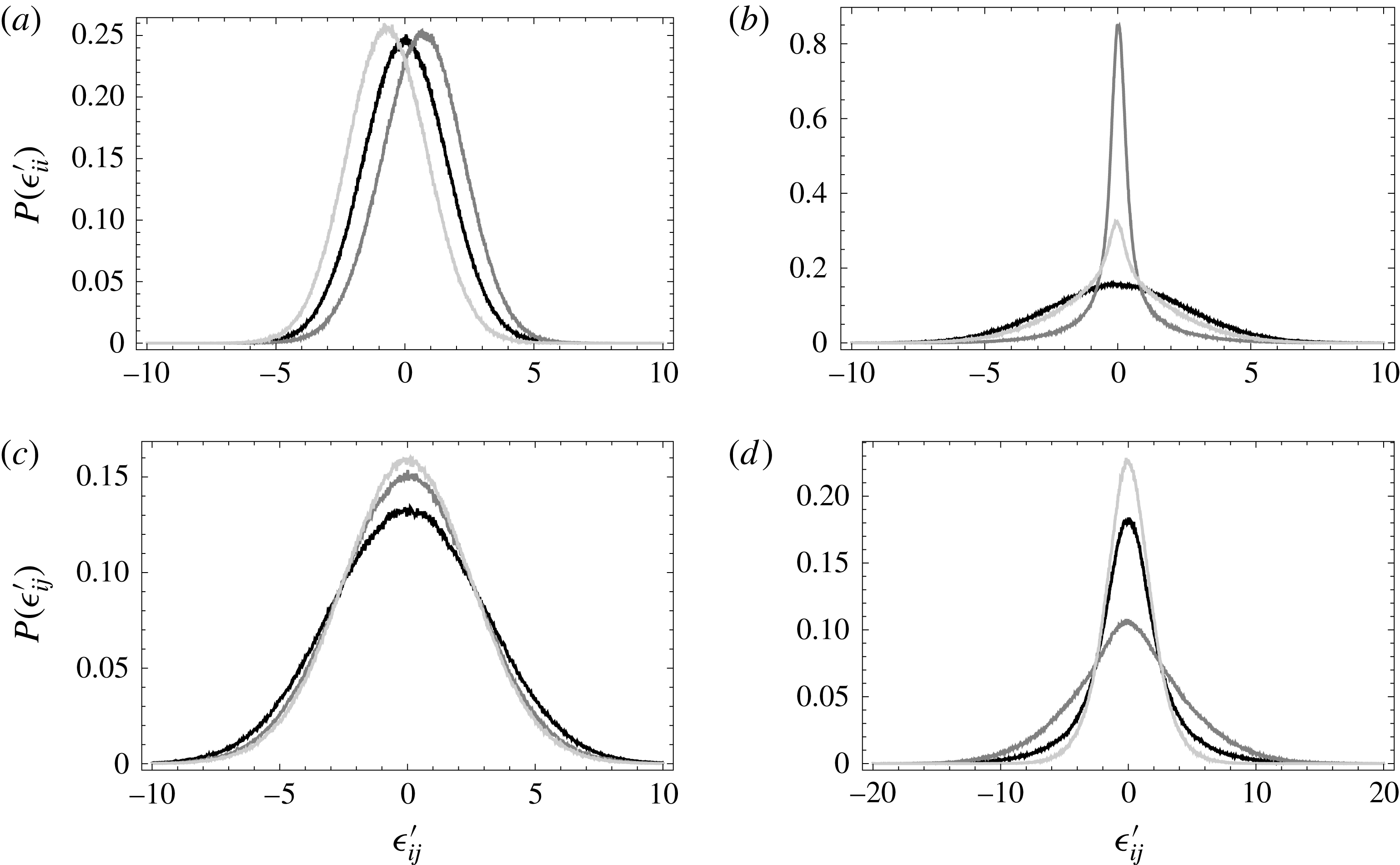
Along with spatial Markovianity of the Lagrangian velocity (and velocity gradient), the remarkably simple deformation structure (strongly decorrelated velocity gradient components) of the VH flow in the Protean frame facilitates explicit solution of the fluid deformation tensor as a CTRW using the methods outlined in § 4. Although not shown here, we observe similar behaviour (spatial Markovianity, strongly decorrelated velocity gradient) for other steady random 3-D flows, including the Kraichnan flow (Kraichnan Reference Kraichnan1970) and a steady random flow defined as
 $\boldsymbol{v}(\boldsymbol{x})\equiv \unicode[STIX]{x1D735}g_{1}(\boldsymbol{x})\times \unicode[STIX]{x1D735}g_{2}(\boldsymbol{x})$
, where
 $g_{1}(\boldsymbol{x})$
,
 $g_{2}(\boldsymbol{x})$
are random steady fields.
The observation of largely uncorrelated velocity gradient components arises as the diagonal and off-diagonal components of the Protean velocity gradient characterise distinctly different deformations (fluid stretching and shear respectively). As the Protean frame separates transverse deformation into orthogonal contracting (
 $\hat{\boldsymbol{e}}_{3}$
) and expanding (
 $\hat{\boldsymbol{e}}_{2}$
) directions, the associated longitudinal
 $\unicode[STIX]{x1D716}_{12}$
and
 $\unicode[STIX]{x1D716}_{13}$
fluid shears are also independent. Similarly, the transverse shear
 $\unicode[STIX]{x1D716}_{23}$
, which characterises the helicity of the flow, is also independent of these longitudinal shears. These observations suggest that the CTRW model of fluid deformation outlined in §§ 3 and 4 can be applied to a wide range of steady random 3-D flows.
Given the difference in Lyapunov exponent for the strong (
 $\unicode[STIX]{x1D713}=\unicode[STIX]{x03C0}/2$
) and weakly (
 $\unicode[STIX]{x1D713}=\unicode[STIX]{x03C0}/64$
) VH flow (
 $\unicode[STIX]{x1D706}\approx 0.679$
,
 $\unicode[STIX]{x1D706}\approx 0.069$
respectively), we expect a larger separation between the advective
 $\unicode[STIX]{x1D70F}_{u}$
and stretching
 $\unicode[STIX]{x1D70F}_{\unicode[STIX]{x1D716}}=1/\unicode[STIX]{x1D716}$
time scales for the less chaotic VH flow,
 $\unicode[STIX]{x1D713}=\unicode[STIX]{x03C0}/64$
. Figure 7 shows the transition from ballistic (
 $t\ll \unicode[STIX]{x1D70F}_{u}$
) to shear-induced stretching (
 $\unicode[STIX]{x1D70F}_{u}\ll t\ll \unicode[STIX]{x1D70F}_{\unicode[STIX]{x1D716}}$
) regimes, where the latter appears to persist beyond
 $\unicode[STIX]{x1D70F}_{\unicode[STIX]{x1D716}}$
for the strongly helical (
 $\unicode[STIX]{x1D713}=\unicode[STIX]{x03C0}/2$
) VH flow. To clearly observe the transition from power-law to exponential stretching as predicted by (4.33), we compare this prediction with numerical calculations of fluid deformation for both cases of the variable helicity flow in figure 8 and the corresponding CTRW (4.24).
Growth of the mean squares
 $A(t)$
(black),
 $B(t)$
(dark grey, blue online),
 $\langle x_{23}(t)^{2}\rangle$
(grey) with time
 $t$
in the ballistic (
 $t\ll \unicode[STIX]{x1D70F}_{u}$
) and shear-induced stretching (
 $\unicode[STIX]{x1D70F}_{u}\ll t\ll \unicode[STIX]{x1D70F}_{\unicode[STIX]{x1D716}}$
) regimes for the VH flow with (a)
 $\unicode[STIX]{x1D713}=\unicode[STIX]{x03C0}/2$
, (b)
 $\unicode[STIX]{x1D713}=\unicode[STIX]{x03C0}/64$
. The analytic scalings
 $\langle x_{ij}(t)^{2}\rangle \sim t^{2}$
from (4.16b-d
), and
 $A(t)\sim t^{6-\unicode[STIX]{x1D6FD}}$
from (4.32) for these regimes are shown by the dashed grey lines.
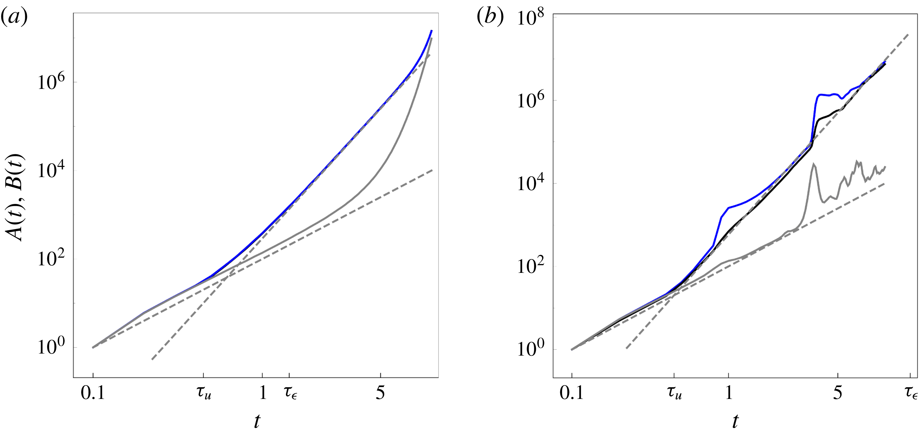
Comparison between analytic prediction of
 $B(t)$
(4.33) (grey dashed line), numerical simulations from the synthetic CTRW (4.24) (black solid line) and deformation in the variable helicity flow (dark grey, blue online) with (a)
 $\unicode[STIX]{x1D713}=\unicode[STIX]{x03C0}/2$
, (b)
 $\unicode[STIX]{x1D713}=\unicode[STIX]{x03C0}/64$
. The dotted line in (b) also depicts the algebraic growth of
 $\langle \unicode[STIX]{x1D60D}_{12}(t)^{2}\rangle \sim t^{2}$
from (4.16b-d
) in the ballistic regime
 $(t\ll \unicode[STIX]{x1D70F}_{u})$
.
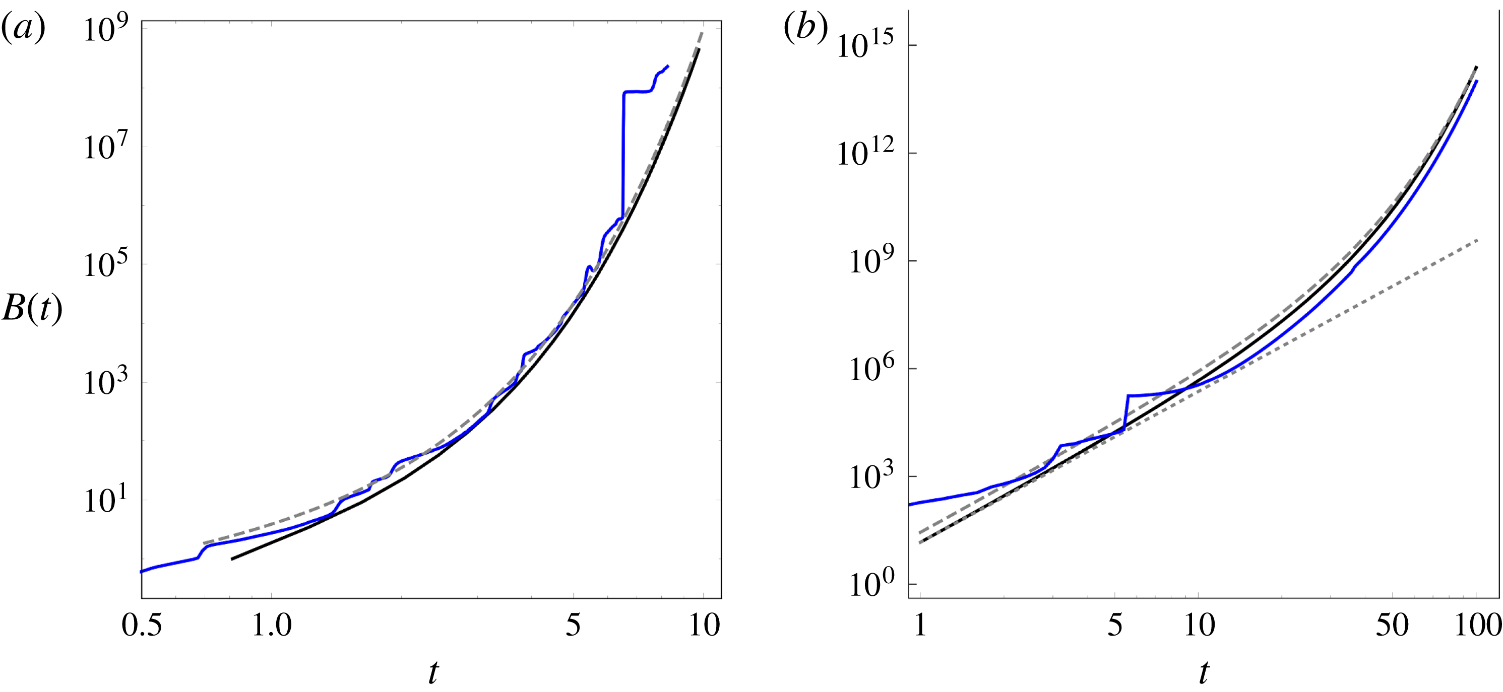
5.1 Evolution of finite-time Lyapunov exponents
From § 4 we may also approximate evolution of the finite-time Lyapunov exponent (FTLE) in chaotic flows as
 $$\begin{eqnarray}\unicode[STIX]{x1D708}(t)\equiv \frac{1}{2t}\ln \unicode[STIX]{x1D707}(t),\end{eqnarray}$$
where
 $\unicode[STIX]{x1D707}(t)$
is the leading eigenvalue of the Cauchy–Green tensor
 $\unicode[STIX]{x1D63E}^{\prime }(t)=\unicode[STIX]{x1D641}^{\prime }(t)^{\top }\boldsymbol{\cdot }\unicode[STIX]{x1D641}^{\prime }(t)$
. Under the approximations
 $\unicode[STIX]{x1D60D}_{11}^{\prime }(t)\sim 0$
,
 $\unicode[STIX]{x1D60D}_{33}^{\prime }(t)\sim 0$
,
 $\unicode[STIX]{x1D60D}_{22}^{\prime }(t)$
,
 $|\unicode[STIX]{x1D60D}_{23}^{\prime }(t)|\sim \exp (\unicode[STIX]{x1D706}t+\unicode[STIX]{x1D70E}_{22}\unicode[STIX]{x1D709}(t))$
,
 $|\unicode[STIX]{x1D60D}_{12}^{\prime }(t)|$
,
 $|\unicode[STIX]{x1D60D}_{13}^{\prime }(t)|\sim t^{2-\unicode[STIX]{x1D6FD}/2}\exp (\unicode[STIX]{x1D706}t+\unicode[STIX]{x1D70E}_{22}\unicode[STIX]{x1D709}(t))$
, where
 $\unicode[STIX]{x1D709}(t)$
is a Gaussian white noise with zero mean and unit variance, then to leading order
 $$\begin{eqnarray}\unicode[STIX]{x1D707}(t)\sim \exp (2\unicode[STIX]{x1D706}t+\unicode[STIX]{x1D70E}_{22}\unicode[STIX]{x1D709}(t))(1+t^{4-\unicode[STIX]{x1D6FD}}).\end{eqnarray}$$
As such, the average FTLE then evolves as
 $$\begin{eqnarray}\langle \unicode[STIX]{x1D708}(t)\rangle \approx \unicode[STIX]{x1D706}+\left(2-\frac{\unicode[STIX]{x1D6FD}}{2}\right)\frac{\ln t}{t},\end{eqnarray}$$
and so as expected the FTLE converges to the infinite-time Lyapunov exponent
 $\unicode[STIX]{x1D706}$
at rate given by the velocity PDF power-law exponent
 $\unicode[STIX]{x1D6FD}$
. We may also compute the variance of
 $\unicode[STIX]{x1D708}(t)$
as
 $$\begin{eqnarray}\unicode[STIX]{x1D70E}_{\unicode[STIX]{x1D708}}^{2}(t)=\langle (\unicode[STIX]{x1D708}(t)-\langle \unicode[STIX]{x1D708}(t)\rangle )^{2}\rangle =\frac{\unicode[STIX]{x1D70E}_{22}^{2}}{t}.\end{eqnarray}$$
As expected, both of these expressions provide accurate estimates of the FTLE mean and variance for all but short times, as reflected in figures 9 and 10 respectively. Here the explicit role of algebraic stretching at times
 $t<\unicode[STIX]{x1D70F}_{\unicode[STIX]{x1D716}}$
is shown to govern convergence of the ensemble average of the FTLE toward its infinite-time value
 $\unicode[STIX]{x1D706}$
.
Comparison between analytic prediction of the mean FTLE
 $\langle \unicode[STIX]{x1D708}(t)\rangle$
(5.7) (grey, dashed), the infinite-time Lyapunov exponent
 $\unicode[STIX]{x1D706}$
(black, dashed) and
 $\langle \unicode[STIX]{x1D708}(t)\rangle$
computed directly (dark grey, blue online) for the variable-helicity flow with (a)
 $\unicode[STIX]{x1D713}=\unicode[STIX]{x03C0}/2$
, (b)
 $\unicode[STIX]{x1D713}=\unicode[STIX]{x03C0}/64$
.
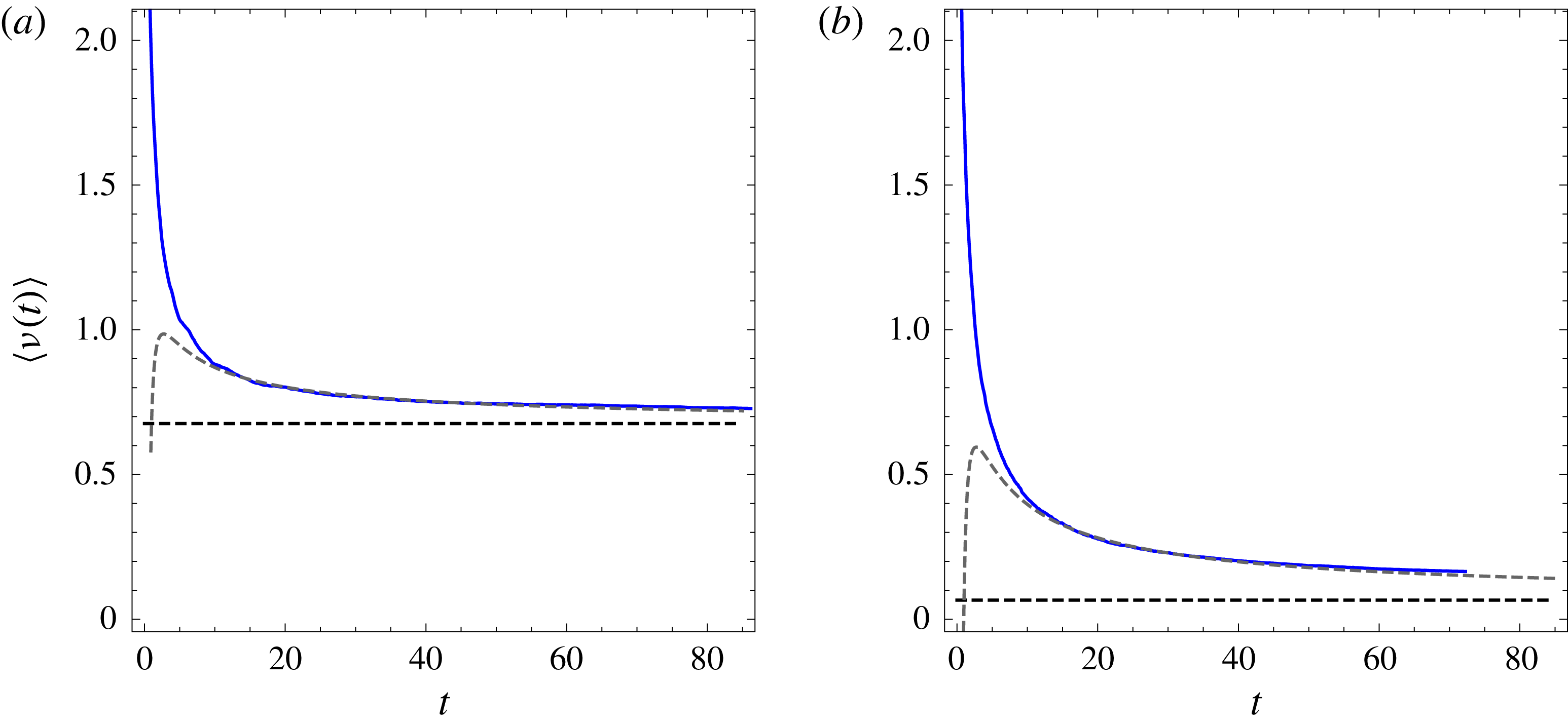
Comparison between analytic prediction of the FTLE variance
 $\langle \unicode[STIX]{x1D70E}_{\unicode[STIX]{x1D708}}^{2}(t)\rangle$
(5.8) (grey, dashed) and
 $\unicode[STIX]{x1D70E}_{\unicode[STIX]{x1D708}}^{2}(t)$
computed directly (dark grey, blue online) for the variable-helicity flow with (a)
 $\unicode[STIX]{x1D713}=\unicode[STIX]{x03C0}/2$
, (b)
 $\unicode[STIX]{x1D713}=\unicode[STIX]{x03C0}/64$
.

6 Conclusions
We have studied the kinematics of fluid deformation in steady 3-D random flows such as pore- and Darcy-scale flows in heterogeneous porous media. We have developed an ab initio stochastic model which predicts evolution of the fluid deformation gradient tensor
 $\unicode[STIX]{x1D641}(t)$
as coupled continuous-time random walk (CTRW) from the velocity and velocity gradient statistics. One important way in which steady flow differs from its unsteady counterpart is that steady flow imposes constraints upon the kinematics of fluid deformation, namely zero mean extensional deformation in the streamwise direction. This constraint then renders fluid deformation in steady flows anisotropic with respect to the velocity direction, and so fluid deformation in steady 3-D flow cannot be characterised in terms of a single scalar quantity. This anisotropy may be characterised in terms of the fluid deformation longitudinal
 $\unicode[STIX]{x1D6EC}_{l}(t)$
and transverse
 $\unicode[STIX]{x1D6EC}_{t}(t)$
to the mean flow direction, which respectively act as inputs to models of longitudinal (Le Borgne et al.
Reference Le Borgne, Dentz and Villermaux2015) and transverse (Lester et al.
Reference Lester, Dentz and Le Borgne2016) mixing in steady random 3-D flows. As such, fluid deformation in such flows cannot be characterised in terms of a single scalar value.
Under an appropriate streamline coordinate system both the velocity gradient and deformation gradient tensor are upper triangular, where the diagonal components correspond to fluid stretching, and the off-diagonal terms correspond to fluid shear. This upper triangular form of the velocity gradient tensor greatly simplifies solution of the deformation gradient tensor ODE, and facilitates derivation of an ab initio stochastic model of fluid deformation in random steady 3-D flows. This approach differs significantly from conventional, empirical stochastic models of fluid deformation.
We apply this framework to several model flows and show that the statistics of the velocity gradient components are remarkably simple, with many components uncorrelated and Gaussian-distributed. Similar to previous studies (Le Borgne et al. Reference Le Borgne, Dentz and Carrera2008a ,Reference Le Borgne, Dentz and Carrera b ; Dentz et al. Reference Dentz, Lester, Borgne and de Barros2016b ) we find that the fluid velocity and velocity gradient components follow a spatial Markov process, which forms the basis for a stochastic model for fluid deformation as a coupled CTRW along streamlines.
We develop analytic solutions to these CTRWs over various temporal regimes in both chaotic and non-chaotic flows, and these solutions show excellent agreement with direct numerical simulations. These solutions provide a concrete means of predicting transverse
 $\unicode[STIX]{x1D6EC}_{t}(t)$
and longitudinal
 $\unicode[STIX]{x1D6EC}_{l}(t)$
fluid deformation in random, steady flows from pointwise velocity statistics. We show that fluid deformation over all temporal regimes only depends upon three statistical parameters: the Lyapunov exponent
 $\unicode[STIX]{x1D706}$
, velocity PDF scaling
 $\unicode[STIX]{x1D6FD}:\lim _{v\rightarrow 0}p_{v}(v)\sim v^{-1+\unicode[STIX]{x1D6FD}}$
, and shear exponent
 $\unicode[STIX]{x1D6FC}:\unicode[STIX]{x1D716}_{12},\unicode[STIX]{x1D716}_{13}\sim v^{5/2-\unicode[STIX]{x1D6FC}}$
. For non-chaotic steady flows (such as isotropic Darcy flow), only
 $\unicode[STIX]{x1D6FD}$
and
 $\unicode[STIX]{x1D6FC}$
need to be quantified. These parameters can be determined directly from high-resolution experimental (e.g. Holzner et al. (Reference Holzner, Morales, Willmann and Dentz2015)) or computational (e.g. de Carvalho et al. (Reference de Carvalho, Morvan, Hargreaves, Oun and Kennedy2017)) studies, or some (such as the velocity PDF scaling) may be estimated from e.g. breakthrough curve data (Tyukhova et al.
Reference Tyukhova, Dentz, Kinzelbach and Willmann2016).
These statistical parameters completely quantify the growth rates of transverse
 $\unicode[STIX]{x1D6EC}_{t}(t)$
and longitudinal
 $\unicode[STIX]{x1D6EC}_{l}(t)$
fluid deformation. This quantitative link between the velocity field statistics and fluid deformation is especially useful for application porous media flows, where recent advances (i) quantitatively link fluid mixing to fluid deformation (de Barros et al.
Reference de Barros, Dentz, Koch and Nowak2012; Le Borgne et al.
Reference Le Borgne, Dentz and Villermaux2015; Lester et al.
Reference Lester, Dentz and Le Borgne2016; Dentz et al.
Reference Dentz, de Barros, Le Borgne and Lester2018), and (ii) quantitatively link medium properties (such as heterogeneity controls in Darcy-scale flow) to velocity field statistics (Fiori et al.
Reference Fiori, Jankovic, Dagan and Cvetkovic2007; Edery et al.
Reference Edery, Guadagnini, Scher and Berkowitz2014; Dentz et al.
Reference Dentz, Kang, Comolli, Le Borgne and Lester2016a
; Tyukhova et al.
Reference Tyukhova, Dentz, Kinzelbach and Willmann2016).
Solution of the governing CTRW uncovers a rich array of fluid deformation behaviour across the various regimes, ranging from linear and power-law to exponential and super-exponential growth. In most cases there are marked differences between longitudinal
 $\unicode[STIX]{x1D6EC}_{l}(t)$
and transverse
 $\unicode[STIX]{x1D6EC}_{t}(t)$
deformation, reflecting the strong deformation anisotropy that results from the constraints inherent to steady 3-D flows. For chaotic flows,
 $\unicode[STIX]{x1D6EC}_{l}(t)$
and
 $\unicode[STIX]{x1D6EC}_{t}(t)$
respectively grow quadratically and linearly with time in the ballistic regime
 $t\ll \unicode[STIX]{x1D70F}_{u}$
, and both of these grow exponentially in the exponential regime
 $t\gg \unicode[STIX]{x1D70F}_{\unicode[STIX]{x1D716}}$
. In the shear-induced stretching regime
 $\unicode[STIX]{x1D70F}_{u}\ll t\ll \unicode[STIX]{x1D70F}_{\unicode[STIX]{x1D716}}$
, transverse deformation grows exponentially, whereas longitudinal deformation transitions from power-law to super-exponential growth due to coupling between shear and stretching. For non-chaotic, steady zero-helicity flows (such as isotropic Darcy flow), transverse and longitudinal fluid deformation both grows algebraically as power-laws via similar mechanisms to that of 2-D steady flows (Dentz et al.
Reference Dentz, Lester, Borgne and de Barros2016b
), namely the intermittency of shear events.
These results uncover and quantify the evolution of transverse and longitudinal fluid deformation in steady random 3-D flows, as illustrated in figure 1. The ad innate stochastic model of fluid deformation identifies and quantifies the statistical parameters of the flow field which govern fluid deformation. The deformation measures
 $\unicode[STIX]{x1D6EC}_{t}(t)$
,
 $\unicode[STIX]{x1D6EC}_{l}(t)$
provide critical inputs to models of fluid mixing and transport in heterogeneous steady flows. This approach provides a means to develop upscaled models of fluid mixing and transport in e.g. porous media flows which may be couched in terms of physical properties of the host medium.
Acknowledgements
F.P.J.deB. acknowledges the support from the National Science Foundation grant no. EAR-1654009. M.D. acknowledges funding from the European Research Council under the European Union’s Seventh Framework Programme (FP7/2007-2013)/ ERC Grant Agreement No. 617511 (MHetScale). T.L.B. acknowledges the support of the European Research Council (ERC) through the project ReactiveFronts (648377) and of the Agence Nationale de la Recherche (ANR) through the project ‘Subsurface Mixing and Reaction’ (ANR-14-CE04-0003).
Appendix A. Analogy to continuous QR decomposition
As the Protean coordinate frame renders the transformed velocity gradient tensor
 $\unicode[STIX]{x1D750}^{\prime }(t)$
upper triangular, this method is directly analogous to the continuous QR decomposition method for a
 $d$
-dimensional autonomous nonlinear dynamical system
 $$\begin{eqnarray}\frac{\text{d}\boldsymbol{x}}{\text{d}t}=\boldsymbol{f}(\boldsymbol{x}),\end{eqnarray}$$
which may be considered as the generalisation of the advection equation
 $\dot{\boldsymbol{x}}=\boldsymbol{v}(\boldsymbol{x})$
for a steady flow field. For a given solution trajectory
 $\boldsymbol{x}(t)$
, the Lyapunov exponents of (A 1) are given by the eigenvalues of the fundamental solutions
 ${\mathcal{Y}}(t)$
of the linear variational equation
 $$\begin{eqnarray}\frac{\text{d}{\mathcal{Y}}}{\text{d}t}={\mathcal{A}}(t)\cdot {\mathcal{Y}}(t),\quad Y(0)=\boldsymbol{I},\end{eqnarray}$$
which is the generalisation of (3.4), where
 ${\mathcal{A}}(t)=\unicode[STIX]{x2202}\boldsymbol{f}/\unicode[STIX]{x2202}\boldsymbol{x}$
is the Jacobian along the trajectory
 $\boldsymbol{x}(t)$
. The continuous QR method considers the decomposition
 $$\begin{eqnarray}{\mathcal{Y}}(t)={\mathcal{Q}}(t)\cdot {\mathcal{R}}(t),\end{eqnarray}$$
where
 ${\mathcal{Q}}(t)$
is orthogonal and
 ${\mathcal{R}}(t)$
upper triangular, and satisfy the auxiliary equations
 $$\begin{eqnarray}\displaystyle & \displaystyle \frac{\text{d}{\mathcal{R}}}{\text{d}t}={\mathcal{A}}^{\prime }\cdot {\mathcal{R}}(t),\quad {\mathcal{R}}(0)=\boldsymbol{I}, & \displaystyle\end{eqnarray}$$
 $$\begin{eqnarray}\displaystyle & \displaystyle \frac{\text{d}{\mathcal{Q}}}{\text{d}t}={\mathcal{Q}}(t)\cdot {\mathcal{H}}(t),\quad {\mathcal{Q}}(0)=\boldsymbol{I}, & \displaystyle\end{eqnarray}$$
where, similar to (3.6)–(3.8),
 $$\begin{eqnarray}\displaystyle & \displaystyle {\mathcal{A}}^{\prime }(t):={\mathcal{Q}}^{\top }(t)\cdot {\mathcal{A}}(t)\cdot {\mathcal{Q}}(t)-{\mathcal{Q}}^{\top }(t)\cdot \dot{{\mathcal{Q}}}, & \displaystyle\end{eqnarray}$$
 $$\begin{eqnarray}\displaystyle & \displaystyle {\mathcal{H}}(t):={\mathcal{Q}}^{\top }(t)\cdot \dot{{\mathcal{Q}}}=\left\{\begin{array}{@{}ll@{}}[{\mathcal{Q}}^{\top }(t)\cdot {\mathcal{A}}(t)\cdot {\mathcal{Q}}(t)]_{ij},\quad & i>j,\\ 0,\quad & i=j,\\ -[{\mathcal{Q}}^{\top }(t)\cdot {\mathcal{A}}(t)\cdot {\mathcal{Q}}(t)]_{ji},\quad & i<j.\end{array}\right. & \displaystyle\end{eqnarray}$$
Hence the evolution equations for the orthogonal and upper triangular matrices
 ${\mathcal{Q}}(t)$
,
 ${\mathcal{A}}^{\prime }(t)$
,
 ${\mathcal{R}}(t)$
for the continuous QR method are directly analogous to the reorientation operator
 $\unicode[STIX]{x1D64C}(t)$
, Protean rate of strain
 $\unicode[STIX]{x1D750}^{\prime }(t)$
and Protean deformation gradient
 $\unicode[STIX]{x1D641}^{\prime }(t)$
tensors for the Protean transform method. However, the actual values differ in that the initial condition for the QR method corresponds to the unrotated frame (
 ${\mathcal{Q}}(0)=\boldsymbol{I}$
), whereas the Protean frame always aligns with the flow direction as per (3.13). Due to the temporal derivative in the reoriented Jacobian (A 6) for the QR decomposition method, solutions to
 ${\mathcal{Q}}(t)$
which render
 ${\mathcal{A}}^{\prime }(t)$
upper triangular are not unique.
Whilst
 ${\mathcal{Q}}(t)$
asymptotically converges to the Protean coordinate frame (due to the dissipative nature of (A 5)), for finite times the continuous QR method does not align with the streamlines of the flow and hence inferences regarding topological and kinematic constraints upon the dynamics do not universally hold. Moreover, for 2-D steady flows (and analogous dynamical systems), the Protean transform provides a simple closed solution (3.13) for
 $\unicode[STIX]{x1D64C}(t)$
, hence it is not necessary to explicitly solve the ODE system (A 5) or employ unitary integration routines (Dieci et al.
Reference Dieci, Russell and Van Vleck1997) to preserve orthogonality of
 ${\mathcal{Q}}(t)$
.
Appendix B. Velocity gradient tensor in orthogonal curvilinear streamline coordinates
It is instructive to contrast the moving Protean coordinate frame with a curvilinear streamline coordinate system, such as that proposed by Finnigan (Reference Finnigan, Moffat and Tsinober1990). This is most easily achieved for zero helicity flows, as they admit lamellar integral surfaces which serve as a convenient coordinate basis (
 $\unicode[STIX]{x1D719}$
,
 $\unicode[STIX]{x1D713}_{1}$
,
 $\unicode[STIX]{x1D713}_{2}$
) with attendant Cartesian unit base vectors
 $\hat{\boldsymbol{e}}_{i}$
defined in (3.54).
These coordinates can also be used to define an orthogonal curvilinear streamline coordinate system. Similar to the Protean frame, in this system the velocity gradient tensor (denoted
 $\unicode[STIX]{x1D750}^{\prime \prime }$
) is somewhat simplified. The unit covariant base vectors
 $\hat{\boldsymbol{g}}_{i}$
of this coordinate system are directly equivalent to the Protean unit vectors
 $\hat{\boldsymbol{e}}_{i}$
, and the coordinates of the curvilinear streamline coordinate system are then
 $$\begin{eqnarray}\unicode[STIX]{x1D709}^{1}=\unicode[STIX]{x1D719}=\unicode[STIX]{x1D719}(x_{1}^{\prime }),\quad \unicode[STIX]{x1D709}^{2}=\unicode[STIX]{x1D713}_{1}=\unicode[STIX]{x1D713}_{1}(x_{2}^{\prime }),\quad \unicode[STIX]{x1D709}^{3}=\unicode[STIX]{x1D713}_{2}=\unicode[STIX]{x1D713}_{2}(x_{3}^{\prime }),\end{eqnarray}$$
where
 $x_{i}^{\prime }$
denote the distance along the coordinate
 $\unicode[STIX]{x1D709}^{i}$
. The differential arc length
 $\text{d}s$
then satisfies
 $\text{d}s^{2}=g_{\unicode[STIX]{x1D6FC}\unicode[STIX]{x1D6FD}}\,\text{d}\unicode[STIX]{x1D709}^{\unicode[STIX]{x1D6FC}}\text{d}\unicode[STIX]{x1D709}^{\unicode[STIX]{x1D6FD}}=\text{d}x_{\unicode[STIX]{x1D6FC}}^{\prime }\,\text{d}x_{\unicode[STIX]{x1D6FD}}^{\prime }$
, and the metric tensor for the orthogonal coordinate system is then
 $$\begin{eqnarray}g_{\unicode[STIX]{x1D6FC}\unicode[STIX]{x1D6FD}}=\left(\begin{array}{@{}ccc@{}}h_{1}^{2} & 0 & 0\\ 0 & h_{2}^{2} & 0\\ 0 & 0 & h_{3}^{2}\\ \end{array}\right).\end{eqnarray}$$
Note that as the components of the covariant
 $g_{\unicode[STIX]{x1D6FC}\unicode[STIX]{x1D6FD}}$
and contravariant
 $g^{\unicode[STIX]{x1D6FC}\unicode[STIX]{x1D6FD}}$
metric tensors transform as
 $$\begin{eqnarray}\displaystyle & \displaystyle g_{ij}^{\prime }(\boldsymbol{x}^{\prime })=\frac{\unicode[STIX]{x2202}x^{k}}{\unicode[STIX]{x2202}x^{\prime i}}\frac{\unicode[STIX]{x2202}x^{l}}{\unicode[STIX]{x2202}x^{\prime j}}g_{kl}^{\prime }(\boldsymbol{x}), & \displaystyle\end{eqnarray}$$
 $$\begin{eqnarray}\displaystyle & \displaystyle g^{\prime ij}(\boldsymbol{x}^{\prime })=\frac{\unicode[STIX]{x2202}x^{\prime i}}{\unicode[STIX]{x2202}x^{k}}\frac{\unicode[STIX]{x2202}x^{\prime j}}{\unicode[STIX]{x2202}x^{l}}g^{\prime kl}(\boldsymbol{x}), & \displaystyle\end{eqnarray}$$
and as
 $g_{\unicode[STIX]{x1D6FC}\unicode[STIX]{x1D6FD}}^{-1}=g^{\unicode[STIX]{x1D6FC}\unicode[STIX]{x1D6FD}}$
, then the scale factors
 $h_{i}$
are then
 $$\begin{eqnarray}h_{i}=\sqrt{\left(\frac{\unicode[STIX]{x2202}x_{1}}{\unicode[STIX]{x2202}\unicode[STIX]{x1D709}^{i}}\right)^{2}+\left(\frac{\unicode[STIX]{x2202}x_{2}}{\unicode[STIX]{x2202}\unicode[STIX]{x1D709}^{i}}\right)^{2}+\left(\frac{\unicode[STIX]{x2202}x_{3}}{\unicode[STIX]{x2202}\unicode[STIX]{x1D709}^{i}}\right)^{2}}=\frac{1}{|\unicode[STIX]{x1D735}\unicode[STIX]{x1D709}^{i}|}=\frac{\unicode[STIX]{x2202}x_{i}^{\prime }}{\unicode[STIX]{x2202}\unicode[STIX]{x1D709}^{i}}.\end{eqnarray}$$
From the isotropic Darcy equation (3.53) and coordinate definitions (B 1), these scale factors can be written without loss of generality as
 $$\begin{eqnarray}h_{1}=\frac{\unicode[STIX]{x2202}x_{1}^{\prime }}{\unicode[STIX]{x2202}\unicode[STIX]{x1D719}}=\frac{k}{v},\quad h_{2}=\frac{\unicode[STIX]{x2202}x_{2}^{\prime }}{\unicode[STIX]{x2202}\unicode[STIX]{x1D713}}=\frac{m}{\sqrt{v}},\quad h_{3}=\frac{\unicode[STIX]{x2202}x_{3}^{\prime }}{\unicode[STIX]{x2202}\unicode[STIX]{x1D701}}=\frac{1}{m\sqrt{v}},\end{eqnarray}$$
where
 $m$
is an arbitrary scalar which quantifies the local spacing of Lamb surfaces. Following Batchelor (Reference Batchelor2000), the components of the velocity gradient tensor
 $\unicode[STIX]{x1D750}^{\prime \prime }$
are then
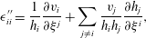 $$\begin{eqnarray}\displaystyle & \displaystyle \unicode[STIX]{x1D716}_{ii}^{\prime \prime }=\frac{1}{h_{i}}\frac{\unicode[STIX]{x2202}v_{i}}{\unicode[STIX]{x2202}\unicode[STIX]{x1D709}^{j}}+\mathop{\sum }_{j\neq i}\frac{v_{j}}{h_{i}h_{j}}\frac{\unicode[STIX]{x2202}h_{j}}{\unicode[STIX]{x2202}\unicode[STIX]{x1D709}^{i}}, & \displaystyle\end{eqnarray}$$
 $$\begin{eqnarray}\displaystyle & \displaystyle \unicode[STIX]{x1D716}_{ij}^{\prime }=\frac{1}{h_{j}}\frac{\unicode[STIX]{x2202}v_{i}}{\unicode[STIX]{x2202}\unicode[STIX]{x1D709}^{j}}-\frac{v_{j}}{h_{i}h_{j}}\frac{\unicode[STIX]{x2202}h_{j}}{\unicode[STIX]{x2202}\unicode[STIX]{x1D701}^{i}}, & \displaystyle\end{eqnarray}$$
and from (B 5) the velocity gradient in the streamline coordinate frame is
 $$\begin{eqnarray}\unicode[STIX]{x1D750}^{\prime \prime }=\left(\begin{array}{@{}ccc@{}}\unicode[STIX]{x1D716}_{11}^{\prime \prime } & \unicode[STIX]{x1D716}_{12}^{\prime \prime } & \unicode[STIX]{x1D716}_{13}^{\prime \prime }\\ \unicode[STIX]{x1D716}_{21}^{\prime \prime } & \unicode[STIX]{x1D716}_{22}^{\prime \prime } & 0\\ \unicode[STIX]{x1D716}_{31}^{\prime \prime } & 0 & \unicode[STIX]{x1D716}_{33}^{\prime \prime }\end{array}\right)=\left(\begin{array}{@{}ccc@{}}\displaystyle \frac{\unicode[STIX]{x2202}v}{\unicode[STIX]{x2202}x_{1}^{\prime }} & \displaystyle \dot{\unicode[STIX]{x1D6FE}}_{2}-\unicode[STIX]{x1D714}_{2} & \displaystyle \dot{\unicode[STIX]{x1D6FE}}_{3}-\unicode[STIX]{x1D714}_{3}\\ \displaystyle \dot{\unicode[STIX]{x1D6FE}}_{2} & \displaystyle -\frac{1}{2}\frac{\unicode[STIX]{x2202}v}{\unicode[STIX]{x2202}x_{1}^{\prime }}+\frac{v}{m}\frac{\unicode[STIX]{x2202}m}{\unicode[STIX]{x2202}x_{1}^{\prime }} & 0\\ \displaystyle \dot{\unicode[STIX]{x1D6FE}}_{3} & 0 & \displaystyle -\frac{1}{2}\frac{\unicode[STIX]{x2202}v}{\unicode[STIX]{x2202}x_{1}^{\prime }}-\frac{v}{m}\frac{\unicode[STIX]{x2202}m}{\unicode[STIX]{x2202}x_{1}^{\prime }}\end{array}\right),\end{eqnarray}$$
where the longitudinal shear rate
 $\dot{\unicode[STIX]{x1D6FE}}_{i}$
and vorticity components
 $\unicode[STIX]{x1D714}_{i}$
(with
 $\unicode[STIX]{x1D74E}=(0,-\unicode[STIX]{x1D714}_{3},\unicode[STIX]{x1D714}_{2})$
) are respectively
 $$\begin{eqnarray}\displaystyle & \displaystyle \dot{\unicode[STIX]{x1D6FE}}_{i}=\frac{\unicode[STIX]{x2202}v}{\unicode[STIX]{x2202}x_{i}^{\prime }}, & \displaystyle\end{eqnarray}$$
 $$\begin{eqnarray}\displaystyle & \displaystyle \unicode[STIX]{x1D714}_{i}=v\frac{\unicode[STIX]{x2202}\ln k}{\unicode[STIX]{x2202}x_{i}^{\prime }}. & \displaystyle\end{eqnarray}$$
From (B 9), the curvilinear velocity gradient satisfies the divergence-free condition
 $\sum _{i}\unicode[STIX]{x1D716}_{ii}^{\prime \prime }=0$
due to the form of the scale factors (B 5). Transverse stretching (as quantified by
 $\unicode[STIX]{x1D716}_{22}^{\prime \prime }$
,
 $\unicode[STIX]{x1D716}_{33}^{\prime \prime }$
) in the zero-helicity flow is due to both velocity fluctuations (as quantified by
 $\unicode[STIX]{x2202}v/\unicode[STIX]{x2202}x_{1}^{\prime }$
) and transient stretching fluctuations (as quantified by
 $\unicode[STIX]{x2202}m/\unicode[STIX]{x2202}x_{1}^{\prime }$
) which are equal and opposite between the 2, 3 directions. These latter fluctuations have zero mean due to the non-chaotic nature of the flow.
By construction of the curvilinear streamline coordinate system the transverse shear components
 $\unicode[STIX]{x1D716}_{23}^{\prime \prime }$
,
 $\unicode[STIX]{x1D716}_{32}^{\prime \prime }$
are both zero, but in contrast to the Protean frame the components
 $\unicode[STIX]{x1D716}_{21}^{\prime \prime }$
,
 $\unicode[STIX]{x1D716}_{31}^{\prime \prime }$
are non-zero, and are respectively equal to the longitudinal shear terms
 $\dot{\unicode[STIX]{x1D6FE}}_{2}$
,
 $\dot{\unicode[STIX]{x1D6FE}}_{3}$
. As these terms are non-zero the corresponding deformation tensor
 $\unicode[STIX]{x1D641}^{\prime \prime }$
is dense. Conversely, in the Protean coordinate frame, the components
 $\unicode[STIX]{x1D716}_{21}^{\prime }$
,
 $\unicode[STIX]{x1D716}_{31}^{\prime }$
are both zero and their contributions are added to the upper triangular terms via the moving coordinate contribution
 $\unicode[STIX]{x1D63C}(t)$
to yield
 $$\begin{eqnarray}\unicode[STIX]{x1D716}_{12}^{\prime }=2\dot{\unicode[STIX]{x1D6FE}}_{2}-\unicode[STIX]{x1D714}_{2},\quad \unicode[STIX]{x1D716}_{13}^{\prime }=2\dot{\unicode[STIX]{x1D6FE}}_{3}-\unicode[STIX]{x1D714}_{3}.\end{eqnarray}$$
The reason for this difference is that the shears
 $\dot{\unicode[STIX]{x1D6FE}}_{i}$
result in a material deformation which is reflected in the curvilinear coordinate system as a contribution to
 $\unicode[STIX]{x1D716}_{i1}^{\prime \prime }$
, but for the rotated Cartesian coordinate system this results as a contribution to
 $\unicode[STIX]{x1D716}_{1i}^{\prime }$
. Note also that the total longitudinal shear (as quantified by
 $\unicode[STIX]{x1D716}_{1i}^{\prime }$
) comprises contributions from pure shear (i.e.
 $\dot{\unicode[STIX]{x1D6FE}}_{i}$
) and streamline curvature (as quantified by vorticity
 $\unicode[STIX]{x1D714}_{i}$
). Hence an orthogonal curvilinear streamline coordinate system does not generate an upper triangular velocity gradient tensor, a result which extends to steady chaotic flows in general.