
1. Introduction
Conventional hydrodynamics can be extended in order to account for multi-phase phenomena. The Young–Laplace model for surface tension besides the Maxwell equation for evaporation/condensation are typically employed. Along with Newton's viscosity law and Fourier's law of heat fluxes, they form linear response approximations for unclosed variables arising from conservation laws. It is well established that these closures become less reliable once strong departures from the equilibrium is observed, e.g. see Wörner (Reference Wörner2012), Schwarzkopf et al. (Reference Schwarzkopf, Sommerfeld, Crowe and Tsuji2011). In practice, this continuum breakdown of multi-phase flows arises in near vacuum conditions and/or miniaturized devices. Plume-droplet interaction in space thrusters (Benson et al. Reference Benson, Levin, Zhong, Gimelshein and Montaser2004), shale gas flows through ultra-tight porous media (Alharthy et al. Reference Alharthy, Nguyen, Teklu, Kazemi and Graves2013) and laser-droplet interaction in high-energy lithography (Hudgins et al. Reference Hudgins, Gambino, Rollinger and Abhari2016) can be mentioned as few examples.
The problem of modelling surface and flux terms can be circumvented by resetting conservation laws in the kinetic theory framework. The latter describes the dynamics by means of the molecular velocity distribution which accounts for the probability that a particle has a certain velocity at a given point in the space–time coordinate. Accordingly, various macroscopic field quantities can be recovered by conditional expectation of molecular quantities. The Boltzmann equation provides an accurate description of the velocity distribution in the dilute gas limit, subject to the molecular chaos assumption (Chapman & Cowling Reference Chapman and Cowling1970; Cercignani Reference Cercignani1988b; Bird Reference Bird1994). By modifying the Boltzmann collision operator, the Enskog equation can be devised for dense gases (Enskog Reference Enskog1922; Van Beijeren & Ernst Reference Van Beijeren and Ernst1973; Resibois Reference Resibois1978). This is achieved by including the volume exclusion in the collision operator and adjusting the collision frequency. As the attractive forces of the molecular potential is represented by the mean-field theory, the Enskog–Vlasov (EV) equation is obtained (Vlasov Reference Vlasov1978). The EV equation can account for liquids, gases and multi-phase flows accurately (Grmela Reference Grmela1971; Karkheck & Stell Reference Karkheck and Stell1981). While the EV equation is adopted as the basis of this study, meso-scale models for multi-phase phenomena can be derived from other routes as well. For example, the Landau-Lifschitz fluctuating hydrodynamics offers a framework to introduce correlations among macroscropic fluxes and, hence, yields improvement over conventional hydrodynamics (Landau & Lifshitz Reference Landau and Lifshitz1959). Following this idea, smoothed-dissipative particle hydrodynamics has been proposed for simulations of multi-phase flows beyond hydrodynamics (Espanol & Revenga Reference Espanol and Revenga2003; Liu, Meakin & Huang Reference Liu, Meakin and Huang2007).
Foremost, direct computation of the velocity distribution from kinetic equations should deal with the high dimensionality of molecular degrees of freedom. Moreover, an accurate discretization of the collision operator has to honour collisional scales which yields stiffness issues near the equilibrium. Finally, long-range interactions described in the EV equation introduces yet another challenge for efficient computations. Spectral and discrete velocity methods have been pursued aiming at an accurate solution of Boltzmann and Enskog equations (see e.g. Broadwell Reference Broadwell1964; Gamba & Tharkabhushanam Reference Gamba and Tharkabhushanam2009; Wu et al. Reference Wu, White, Scanlon, Reese and Zhang2013; Wu, Zhang & Reese Reference Wu, Zhang and Reese2015; Wu et al. Reference Wu, Liu, Reese and Zhang2016). The problem of high dimensionality of kinetic systems can be relaxed by approximating the velocity distribution via a finite number of moments. These so-called moment methods which are applicable for flows not too far from the equilibrium have been devised using Grad's ansatz, Chapman–Enskog expansion, maximum entropy solution and quadrature methods (see, e.g. Kremer & Rosa Reference Kremer and Rosa1988; Torrilhon Reference Torrilhon2016; Heylmun et al. Reference Heylmun, Kong, Passalacqua and Fox2019; Struchtrup & Frezzotti Reference Struchtrup and Frezzotti2019; Wang et al. Reference Wang, Wu, Ho, Li, Li and Zhang2020).
Alternatively, the curse of high dimensionality can be avoided by evolving samples of the distribution according to the underlying stochastic process; at the cost of introducing statistical noise. Direct simulation Monte-Carlo (DSMC) introduced by Bird (Reference Bird1963) is the most popular particle algorithm for rarefied gas flow simulations. By adopting the same principles, Montanero & Santos (Reference Montanero and Santos1997a), Alexander, Garcia & Alder (Reference Alexander, Garcia and Alder1995), Hadjiconstantinou, Garcia & Alder (Reference Hadjiconstantinou, Garcia and Alder2000), Frezzotti (Reference Frezzotti1997b) and Frezzotti, Barbante & Gibelli (Reference Frezzotti, Barbante and Gibelli2019) extended the DSMC algorithm for dense flows. However, as DSMC can successfully circumvent the high-dimensionality issue by resetting the kinetic system into the Monte-Carlo framework, it inherits stiffness of the collision operator near the equilibrium. This fundamental issue lies on the fact that the stochastic process resulting from the collision operator is not continuous in the velocity space. Thus, time step sizes smaller than the mean collision time and spatial discretization smaller than the mean free path should be adopted.
The high-computational cost associated with dense collisions motivated Jenny, Torrilhon & Heinz (Reference Jenny, Torrilhon and Heinz2010) to introduce a particle approach based on the Fokker–Planck (FP) approximation of the Boltzmann equation. The main idea behind the FP model is to describe the jump process resulting from the collision operator by an equivalent drift-diffusion process. Hence, the resulting stochastic paths become continuous and, thus, the discretization constraints become more relaxed in comparison to DSMC type approaches. Further improvements of the FP model led to a continuous stochastic description of dense gases on the basis of the Enskog equation (Sadr & Gorji Reference Sadr and Gorji2017). The FP model for dense gases (DFP) is constructed such that relaxation rates of various production terms of the Enskog collision operator, as well as the collisional transfer of conserved quantities during the collision, are honoured.
At a different front, the computation of long-range interaction based on the mean-field limit can introduce further complexities due to the long tail of the molecular potential. In contrast to kernel based estimation of long-range interactions (Piechór Reference Piechór1994; Frezzotti, Gibelli & Lorenzani Reference Frezzotti, Gibelli and Lorenzani2005; Frezzotti et al. Reference Frezzotti, Gibelli, Lockerby and Sprittles2018), a global solution algorithm can be devised as shown by Sadr & Gorji (Reference Sadr and Gorji2019). First the attractive part of the molecular potential can be approximated accurately via Green's function associated with an elliptic partial differential equation (PDE). The resulting screened-Poisson equation (SP) then can be adopted in order to approximate the Vlasov integral. Unlike density expansion methods which are local and require high regularity of the density field (Korteweg Reference Korteweg1901; He & Doolen Reference He and Doolen2002), the solution offered by the SP model retains global features of the Vlasov integral and allows for strong variations of the density field.
In this study a solution algorithm is devised, which combines an accurate continuous description of the molecular collisions along with an efficient estimation of long-range interactions. The former is achieved by the DFP approximation of the Enskog equation, whereas the latter follows the SP model for the Vlasov integral. First, in § 2 the kinetic theory as a mathematical model of multi-phase flows is described. In particular, the Enskog collision operator and the Vlasov integral are reviewed in §§ 2.1 and 2.2, respectively. Then, the FP approximation of the Enskog equation along with the SP model of long-range forces are reviewed in §§ 3.1 and 3.2, respectively. Next, an efficient particle Monte-Carlo solution algorithm for the Fokker-Planck-Poisson (DFP-SP) model suitable for multi-phase flows is assembled in § 4.
The resulting DFP-SP model then is validated in § 5 by studying evaporation of droplets in equilibrium and non-equilibrium settings. As the benchmark, numerical simulation based on the EV equation is obtained by combining the Enskog simulation Monte-Carlo derived by Montanero & Santos (Reference Montanero and Santos1997b) for collisions, and Legendre–Gauss quadrature for the Vlasov integral. Next, the DFP-SP model is adopted to study inverted temperature gradients and spinodal decomposition problems in §§ 6 and 7, respectively. For the former, the heat transfer between two liquid slabs kept at a background gas is studied in a one-dimensional geometry. The results are compared with respect to benchmark EV solutions. By investigation of the single droplet evaporation, further insight is gained with respect to the origin of inverted temperature gradient phenomenon. Finally gas-droplet decomposition in a meta-stable setting known as the spinodal decomposition is studied in two- and three-dimensional settings. The simulation results are found to exhibit Lifschitz–Slyozov growth rates for the droplets. The validation study along with detailed simulation results provided for inverted temperature gradient and spinodal decomposition confirm efficiency and accuracy of the proposed DFP-SP model. The paper concludes in § 8, where an outline of future improvements is discussed.
2. Review of the EV kinetic model
As the number of molecules which constitute a typical fluid portion is immense, it is more natural to apply a statistical approach if we are interested in the macroscopic behaviour of the system. The kinetic theory provides a description of the flow by means of the molecular distribution. Consider an ensemble of random particles with translational degrees of freedom. The state of the ensemble is fully determined by random variables  $X(t)\in \mathbb {R}^3$ and
 $V(t)\in \mathbb {R}^3$ which account for position and velocity of a sample at time
 $t\in \mathbb {R}^+$, respectively. Equivalently, we can deduce the single-particle velocity distribution at position
 $x$ and velocity
 $v$ by
 \begin{equation} \mathcal{F}(v,x,t)= \mathcal{M}\mathbb{E}[\delta(x-X(t))\delta (v-V(t))], \end{equation}
where  $\mathbb {E}[\cdot ]$ is the expectation,
 $\delta (\cdot )$ denotes the Dirac delta and
 $\mathcal {M}$ accounts for the total mass of the system (see, e.g. Gorji Reference Gorji2014). In absence of boundary effects, the distribution
 $\mathcal {F}$ evolves due to the inter-molecular interactions. For our system of particles with molecular mass
 $m$, consider the Sutherland molecular potential
 \begin{equation} \phi(r)= \left\{\begin{array}{@{}ll} +\infty, & r<\sigma,\\ \phi_0 \left(\dfrac{\sigma}{r} \right)^6, & r \geq \sigma, \end{array}\right. \end{equation}
where  $r$ is the distance between any two particles,
 $\sigma$ indicates the effective diameter and
 $\phi _0$ is a scaling factor. In principle, for a given inter-molecular potential, the Liouville equation offers evolution of the multi-particle distribution as shown by Cercignani (Reference Cercignani1988a). However, if further simplifications are adopted, i.e. the mean-field limit for long-range interactions along with the molecular chaos assumption, a closed-form equation for
 $\mathcal {F}$ can be deduced (Grmela Reference Grmela1971; Karkheck & Stell Reference Karkheck and Stell1981; Cercignani Reference Cercignani1988a). Contributions of short-range interactions to the evolution of
 $\mathcal {F}$ can be captured by considering an elastic collision operator, whereas the
 $N$-body problem arising from the long-tail interaction can be approximated by the mean-field limit (Vlasov Reference Vlasov1978). Hence, the EV equation
 \begin{equation} \frac{\partial \mathcal{F}}{\partial t} + \frac{\partial (\mathcal{F} v_i)}{\partial x_i} - \frac{1}{m} H_i \frac{\partial \mathcal{F}}{\partial v_i} = S^{{Ensk}}(\mathcal{F}),\end{equation}
can be derived, where the Enskog collision operator  $S^{{Ensk}}(\mathcal {F})$ accounts for the contribution of molecular collisions. Furthermore, the conservative force field
 $H_i :={\partial \varPhi }/{\partial x_i}$ accounts for long-range attraction and follows the gradient of the mean-field potential
 $\varPhi$. Here and henceforth, the Einstein summation convention is used to economize our notation.
It is important to emphasize that the underlying assumptions behind the conventional EV equation makes it constrained to monatomic single species flows at moderate densities. However, validation studies in comparison with molecular dynamics (MD) simulations in various non-equilibrium scenarios motivates its further use and development for a broad range of multi-phase flow processes (Frezzotti Reference Frezzotti1997a; Kon, Kobayashi & Watanabe Reference Kon, Kobayashi and Watanabe2014; Frezzotti et al. Reference Frezzotti, Nedea, Markvoort, Spijker and Gibelli2008, Reference Frezzotti, Gibelli, Lockerby and Sprittles2018).
In follow-up subsections, first we review the Enskog collision operator and next a short description on the mean-field potential  $\varPhi$ is provided.
2.1. Enskog operator
The short-range interactions have two main influences on evolution of the velocity distribution: relaxation towards equilibrium and transport of conserved quantities. Note that the latter is only the case for dense flows. The Enskog collision operator derived by Enskog (Reference Enskog1922) and then modified by Van Beijeren & Ernst (Reference Van Beijeren and Ernst1973), Resibois (Reference Resibois1978) is an extension of the Boltzmann collision operator by including the volume of particles. The standard Enskog collision operator for hard-sphere collisions reads as
 \begin{align} S^{{Ensk}}(\mathcal{F}) &= \frac{1}{m} \int_{\mathbb{R}^{3}} \int_{0}^{2{\rm \pi} } \int_0^\sigma \left[ Y \left( {x}+\frac{1}{2} \sigma \hat{k}\right) \mathcal{F}( {v}^*, {x})\mathcal{F}( {v}^*_1,\ {x}+\sigma \hat{k})\right. \nonumber\\ &\quad -\left.Y \left( {x}-\frac{1}{2} \sigma \hat{k}\right)\mathcal{F}( {v}, {x})\mathcal{F}( {v}_1, {x}-\sigma \hat{k}) \right] g \mathcal{H}( g_i \hat{k}_i) \hat{b} \, \textrm{d}\hat{b} \, \textrm{d} \hat{\epsilon}\, \textrm{d} {v}_1, \end{align}
where  $\hat {k}$ indicates the unit vector connecting the centre of a particle to its colliding pair with subscript
 $(\cdot )_1$,
 $\mathcal {H}(\cdot )$ is the Heaviside step function,
 $g$ is the relative velocity of colliding pair, and
 $\hat {b}$ and
 $\hat {\epsilon }$ are the impact parameter and scattering angle, respectively. Note that in the case of the hard-sphere potential the impact parameter relates to deflection angle
 $\chi$ via
 $\hat {b}=\sigma \cos (\chi /2)$, where
 $\chi \in [0,{\rm \pi} )$. For further details of the Enskog and Boltzmann collision operators, see, e.g. Chapman & Cowling (Reference Chapman and Cowling1970), Hirschfelder, Bird & Curtiss (Reference Hirschfelder, Bird and Curtiss1964) and Bird (Reference Bird1994).
In comparison to the dilute limit the Enskog collision operator admits a diameter distance between the colliding pair as well as an increase in collision rate by  $Y$. The standard Enskog equation estimates the pair correlation factor
 $Y$ to be a function of density at the contact of colliding spheres, which can be chosen such that the correct equilibrium pressure is guaranteed. By means of the Carnahan–Starling equation of state, we get
 $$\begin{gather} Y = \frac{1}{2}\frac{2-\eta}{(1-\eta)^3}, \end{gather}$$
 $$\begin{gather}\textrm{with}\quad \eta := nb/4, \end{gather}$$
where  $b:=2 {\rm \pi}\sigma ^3/3$ is the second virial coefficient (Carnahan & Starling Reference Carnahan and Starling1969). Furthermore, the number density is denoted by
 $n$ which gives the density
 $\rho =mn$.
In addition to the curse of dimensionality associated with  $\mathcal {F}$, the increase of collision rate along with the non-locality of collision operator lead to further computational complications. Although direct Monte-Carlo particle methods can cope with the high dimensionality at the cost of introducing statistical noise, they inherit the issues with non-locality of the collision step along with resolving collisional scales.
2.2. Vlasov integral
By applying the mean-field limit, the attractive force of (2.3) is represented as the derivative of the Vlasov integral
 \begin{equation} \varPhi(x,t) = \int_{r>\sigma} \phi(r) n(y,t)\, {\textrm{d} y},\end{equation}
where  $r:=|y-x|$ and
 $| \cdot |$ denotes Euclidean distance. Although the Vlasov integral can be computed using quadrature rules as discussed in Appendix A.2, long tails and mesh refinement near
 $r=\sigma$ make the numerical integration expensive in practice.
3. Fokker-Planck-Poisson model
Here a detailed description of the Fokker-Planck-Poisson model covering both short- and long-range interactions is discussed. First, in § 3.1 the FP approximation of collisions in dense gases is reviewed. Next, we explain the elliptic model that captures the long-range forces globally, by means of the SP equation in § 3.2.
3.1. Short-range interactions
The computational cost associated with resolving the Enskog collision operator, i.e. right-hand side of (2.3), can be decoupled from collisional scales once the underlying jump process is described by an equivalent continuous process. Furthermore, if the stochastic paths generated by the latter process depends only on local moments of the distribution, efficient cell-based parallelization can be exploited.
Let us consider an Itô drift-diffusion process as a general prototype of such a continuous process. Then, the task becomes to find a drift-diffusion closure such that the resulting single-particle velocity distribution evolves consistent with the underlying jump process, up to a desired degree of moments. From a physical point of view, such a drift-diffusion process expresses all the forces acted on a sample particle into a portion which is correlated to the particle's state and a remainder being purely random. The former is governed by the drift whereas the latter is controlled by the diffusion coefficient.
Consider the position and velocity of particles given by random variables  $(X(t),V(t))$. Suppose that the evolution of particles can be modelled through stochastic differential equations (SDEs) with drift
 $A$ and diffusion
 $D$ in velocity space, as well as a spatial drift
 $\hat {A}$ in the physical space

where  $i\in \{1,2,3\}$. Here
 $\textrm {d} W_{t,i}:=W_i(t+\textrm {d} t)-W_i(t)$ indicates the increment of the Wiener process for the
 $i$th component of particle velocity which follows a Gaussian distribution with zero mean and variance of
 $\textrm {d} t$, i.e.
 $\textrm {d} W_{t,i}\sim \mathcal {N}(0,\textrm {d} t)$. Using Itô's lemma, evolution of the corresponding
 $\mathcal {F}$ follows a FP equation of the form
 \begin{equation} \dfrac{\partial \mathcal{F}}{\partial t} + \dfrac{\partial (\mathcal{F} v_i)}{\partial x_i} = S^{{DFP}}(\mathcal{F}),\end{equation}
where
 \begin{equation} S^{{DFP}} (\mathcal{F}) = \underbrace{-\frac{ \partial (\mathcal{F} A_i )}{\partial v_i} +\frac{1}{2}\frac{\partial^2 ( D^2 \mathcal{F}) }{\partial v_i \partial v_i}}_{\text{relaxation rates}} \underbrace{-\frac{ \partial (\mathcal{F} \hat{A}_i )}{\partial x_i}}_{\text{col. transfer}}.\end{equation}
For a relationship between the FP equation and SDEs, see, e.g. Oksendal (Reference Oksendal2013). The drift  $A$ and diffusion
 $D$ allow us to fix the rate at which non-conservative velocity moments including the kinetic stress tensor
 \begin{equation} {\rm \pi}_{ij}^{kin} =\int_{\mathbb{R}^3} v_{\langle i}^\prime v_{j \rangle}^\prime \mathcal{F} \, \textrm{d} v \end{equation}
and the kinetic heat flux vector
 \begin{equation} q_{i}^{kin} = \tfrac{1}{2} \int_{\mathbb{R}^3} v_i^\prime v_j^\prime v_j^\prime \mathcal{F} \, \textrm{d} v \end{equation}
relax due to collisions. Note that subscript  $\langle . \rangle$ denotes the deviatoric part of the tensor and
 $v^\prime :=v-U$ is the fluctuating velocity with
 $U=(1/\rho )\int v \mathcal {F} \, \textrm {d} v$ being the bulk velocity.
The spatial drift  $\hat {A}$ accounts for the collisional transfer resulting from dense effects. From a physical point of view, the introduced drift in the position update corrects the particle position due to the volume exclusion. In other words, in the absence of such a correction the described SDEs only provide the velocity and position of particles with a vanishing diameter.
By considering the spatially homogeneous setting, we fix  $A$ and
 $D$ such that the resulting moment system remains consistent with the Enskog equation up to the heat fluxes. Accordingly, the constraints
 \begin{gather} \int_{\mathbb{R}^{3}} v^\prime_{\langle i} v^\prime_{ j \rangle} S^{{DFP}}(\mathcal{F})\, \textrm{d} {v} = \int_{\mathbb{R}^{3}} v^\prime_{\langle i} v^\prime_{ j \rangle} S^{{Ensk}}(\mathcal{F})\, \textrm{d} {v} \quad \text{and} \end{gather}
 \begin{gather}\int_{\mathbb{R}^{3}} v^\prime_{ i} v^\prime_{ j} v^\prime_{ j} S^{{DFP}} (\mathcal{F})\, \textrm{d} {v} = \int_{\mathbb{R}^{3}} v^\prime_{ i} v^\prime_{ j} v^\prime_{ j} S^{{Ensk}} (\mathcal{F})\, \textrm{d} {v} \end{gather}
are devised. In order to obtain a tractable expression for the right-hand side of (3.6) and (3.7), here we approximate moments of the Enskog collision operator by applying Maxwell molecules. Therefore, we get
 \begin{gather} \int_{\mathbb{R}^3} \left( A_i v^\prime_j + A_j v^\prime_i - \frac{2}{3} A_k v^\prime_k \delta_{ij} + \frac{2}{3} \delta_{ij} D^2 \right) \mathcal{F} \, \textrm{d} v ={-} Y \frac{p^{{kin}}}{\mu^{{kin}} } {\rm \pi}_{ij}^{{kin}} \quad \textrm{and} \end{gather}
 \begin{gather}\int_{\mathbb{R}^3} ( A_i v^\prime_j v^\prime_j + 2 A_j v^\prime_j v^\prime_i ) \mathcal{F} \, \textrm{d} v ={-} Y \frac{2}{3} \frac{p^{{kin}}}{\mu^{{kin}} } q_i^{{kin}}. \end{gather}
Note that here the kinetic ideal gas viscosity coefficient is denoted by  $\mu ^{{kin}}$, the ideal gas equilibrium pressure is
 $p^{{kin}}=nk_b T$ and the superscript
 $(\cdot )^{kin}$ indicates the kinetic contribution.
Next, the extra transport resulting from spatial dependencies of the Enskog operator is accounted by the spatial drift. The degrees of freedom in extra streaming induced by  $\hat {A}$ are set such that the resulting FP model remains consistent with the Enskog collision operator up to the heat fluxes. Let
 $\psi =[1,v_i, v_jv_j/2]^\textrm {T}$, by the Taylor expansion of
 $\mathcal {F}(x\pm \sigma \hat {k})$ and
 $Y(x\pm \sigma \hat {k}/2)$ around
 $x$, the conservative moments of the Enskog collision operator can be formulated as fluxes
 \begin{gather} \int_{\mathbb{R}^3} \psi_l S^{{Ensk}}(\mathcal{F})\, \textrm{d} {v} ={-} \dfrac{\partial \varPsi^\phi_{lk}}{\partial x_k}, \quad \textrm{where} \end{gather}
 \begin{gather}
\hspace{-4pc}\varPsi_{lk}^\phi =
\frac{Y \sigma}{2m} \iiiint (\psi^*_l-\psi_l) \mathcal{F}
\mathcal{F}_1 \hat{k}_k g \hat{b} \, \textrm{d} \hat{b} \,
\textrm{d} \hat{\epsilon}\, \textrm{d} {v}_1\, \textrm{d}
{v} \nonumber\\ \hspace{4.5pc} +\frac{Y \sigma^2}{4m} \iiint
(\psi^*_l-\psi_l) \hat{k}_k \hat{k}_j \mathcal{F}
\mathcal{F}_1 \frac{\partial}{\partial x_j} \ln
\left(\frac{\mathcal{F}}{\mathcal{F}_1}\right) g \hat{b} \,
\textrm{d} \hat{b} \, \textrm{d} \hat{\epsilon}\,
\textrm{d} {v}_1\, \textrm{d} {v} \nonumber\\ \hspace{-13pc} +
\cdots ,
\end{gather}
as shown by Chapman & Cowling (Reference Chapman and Cowling1970). In particular, the corrections accounted by the spatial drift  $\hat {A}$ become
 \begin{equation} \frac{\partial }{\partial x_k} \int_{\mathbb{R}^{3}} \hat{A}_k \psi_l \mathcal{F} \, \textrm{d} v \approx \dfrac{\partial \varPsi^\phi_{lk}}{\partial x_k} \quad \textrm{for }l=1,\ldots,\dim( \psi). \end{equation}
Assuming Maxwellian for  $\mathcal {F}$ in
 $\partial _{x_j} \ln ({\mathcal {F}}/{\mathcal {F}_1})$ inside the second integral of (3.11) and ignoring higher-order terms, a closure for collisional transfer can be derived,
 \begin{gather} \int_{\mathbb{R}^3} \hat{A}_i \mathcal{F} \, \textrm{d} v = 0, \end{gather}
 \begin{gather}\int_{\mathbb{R}^3} \hat{A}_i v_j \mathcal{F} \, \textrm{d} v = nbY(p^{kin}\delta_{ij}+2/5{\rm \pi}^{kin}_{ij}) -w\left(\frac{\partial U_k}{\partial x_k}\delta_{ij}+\frac{5}{6}\frac{\partial U_{\langle i}}{ \partial x_{j \rangle}}\right), \end{gather}
 \begin{gather}\text{and} \quad \frac12 \int_{\mathbb{R}^3} \hat{A}_i v_j v_j \mathcal{F} \, \textrm{d} v = \frac{3}{5} nbY q_i^{{kin}} - c_v w \frac{\partial T}{\partial x_i}. \end{gather}
Here  $c_v=3 k_b /(2m)$ is the heat capacity at constant volume,
 \begin{equation} w = (nb)^2 Y \sqrt{mk_bT}/({\rm \pi}^{3/2} \sigma^2)\end{equation}
is the second viscosity coefficient,  $T= \int _{\mathbb {R}^3} v^\prime _j v^\prime _j \mathcal {F} \, \textrm {d} v/(3nk_b)$ is the temperature and
 $k_b$ denotes the Boltzmann constant.
A simple set of polynomial ansatz to fulfil (3.8) and (3.9) in combination with (3.13)–(3.15) is adopted. Following Sadr & Gorji (Reference Sadr and Gorji2017), the cubic FP model for dense collisions
 \begin{gather} A_i=c_{ij}v^\prime_j+\gamma_i\left(v^\prime_jv^\prime_j-\frac{3k_bT}{m}\right)+\varLambda \left(v^\prime_iv^\prime_j v^\prime_j-\frac{2q^{kin}_i}{\rho}\right), \end{gather}
 \begin{gather}D =\sqrt{\frac{k_bT}{\tau m}}, \end{gather}
 \begin{gather}\textrm{and} \quad \hat{A}_i = \hat{c}_{ij} v^\prime_j + \hat{\gamma}_i \left(v^\prime_j v^\prime_j - \frac{3k_bT}{m}\right) + \hat{\varLambda} \left( v^\prime_i v^\prime_j v^\prime_j - \frac{2q^{kin}}{\rho} \right) \end{gather}
is devised. The time scale  $\tau$ is set using kinetic scales
 $\tau =2\mu ^{{kin}}/(p^{{kin}}Y)$. The coefficients of the tensors
 $c$ and
 $\hat {c}$ along with the vectors
 $\gamma$ and
 $\hat {\gamma }$ need to be computed based on velocity moments. The cubic term is responsible to make sure that the SDEs remain stable (see Risken Reference Risken1989; Gorji, Torrilhon & Jenny Reference Gorji, Torrilhon and Jenny2011). The coefficients of the cubic terms are set to
 \begin{gather} \varLambda={-}\frac{|\det (u_{ij})|}{ (u^{(2)})^4 \tau }\quad \textrm{and} \end{gather}
 \begin{gather}\hat{\varLambda} ={-} \epsilon \frac{nbY}{k_b T/m }, \end{gather}
where  $\epsilon =10^{-3}$,
 $\det (\cdot )$ indicates the determinant and
 \begin{equation} u_{i_1\ldots i_n}^{(k)}:=\frac{1}{\rho}\int_{\mathbb{R}^{3}}| {v^\prime}|^kv^\prime_{i_1}v^\prime_{i_2}\ldots v^\prime_{i_n}\mathcal{F}\, \textrm{d} v; \quad i_k\in\{1,2,3\}. \end{equation}
By substituting the ansatz for  $A$ and
 $D$ in equations for the relaxation rates (3.8) and (3.9), one can show that
 \begin{align} &c_{ik}u^{(0)}_{kj}+c_{jk}u^{(0)}_{ki}+\gamma_iu^{(2)}_{j}+\gamma_ju^{(2)}_{i}={-}2\varLambda u^{(2)}_{ij} \quad \textrm{and} \end{align}
 \begin{align} &c_{ij}u^{(2)}_j+2c_{jk}u^{(0)}_{ijk}+\gamma_i(u^{(4)}-(u^{(2)})^2) +2\gamma_j(u^{(2)}_{ij}-u^{(2)}u_{ij}) \nonumber\\ &\quad ={-}\varLambda (3u^{(4)}_i-u^{(2)}_iu^{(2)}-2u^{(2)}_ju^{(0)}_{ij}) +\frac{5}{6}\frac{Yp^{kin}}{\mu^{{kin}}}q_i^{kin}. \end{align}
Equivalently, for  $\hat {A}$, we get
 \begin{gather} \hspace{-9.5pc}\hat{c}_{jk}{\rm \pi}_{ik}^{kin}+\hat{c}_{ji}p^{kin}+2\hat{\gamma}_jq_i^{kin} ={-}\rho \hat{\varLambda} u^{(2)}_{ij}\\ + nbY(p^{kin}\delta_{ij}+2/5{\rm \pi}^{kin}_{ij}) -w\left(\frac{\partial U_k}{\partial x_k}\delta_{ij}+ \frac{5}{6}\frac{\partial U_{\langle i}}{ \partial x_{j \rangle}}\right) \quad \textrm{and} \end{gather}
 \begin{gather} \hat{c}_{ij} q_j^{kin} +\frac{1}{2}\rho \hat{\gamma}_i ( u^{(4)} - (u^{(2)}) ^2) =\frac{3}{5}nbYq_i^{kin} - w c_v\frac{\partial T}{\partial x_i} - \frac{1}{2}\rho \hat{\varLambda} (u^{(4)}_i - u^{(2)}_i u^{(2)} ),\end{gather}
where  $i,j,k\in \{1,2,3\}$. The unknowns
 $c, \gamma , \hat {c}$ and
 $\hat {\gamma }$ can be found by solving two linear systems,
 \begin{equation} A_v \begin{pmatrix} c_{1,1}\\ \vdots\\ c_{3,3} \\ \gamma_{1}\\ \vdots\\ \gamma_{3} \end{pmatrix} = b_v \quad \mathrm{and} \quad A_x \begin{pmatrix} \hat{c}_{11}\\ \vdots\\ \hat{c}_{3,3} \\ \hat{\gamma}_{1}\\ \vdots\\ \hat{\gamma}_{3} \end{pmatrix}= b_x,\end{equation}
where the matrices  $A_v$ and
 $A_x$ together with the right-hand side matrices
 $b_v$ and
 $b_x$ are read from (3.23) and (3.24) and (3.25) and (3.26), respectively.
As shown in Sadr & Gorji (Reference Sadr and Gorji2017), the DFP model, besides reproducing near-equilibrium results, accurately captures non-equilibrium effects within the transition regime for moderate densities. Specifically, we expect a reasonable accuracy for the DFP model in the range of density where  $nb\leq 1$.
3.2. Long-range interactions
The contribution of the long-range molecular potential in the evolution of molecular velocity distribution function can be accurately accounted by the Vlasov mean-field limit. Although the direct numerical evaluation of long-ranged forces through the Vlasov integral is grid-independent however, it can lead to high-computational costs due to a relatively large support of the kernel. In practice, global solutions over a spatial discretization turn out to be less expensive (Sadr & Gorji Reference Sadr and Gorji2019). Consider an approximation  $\tilde {\phi }(r)$ to the attractive part of molecular potential
 $\phi (r)$ where
 \begin{gather} \tilde{\phi}( r) = a G( r) \hspace{0.5cm} \text{and} \end{gather}
 \begin{gather}G( r) = \frac{\textrm{e}^{-\lambda r}}{4 {\rm \pi}r}. \end{gather}
An estimate of fitting parameters  $a$ and
 $\lambda$ can be obtained by solving an optimization problem of the type
 \begin{equation} (a,\lambda) = \underset{r \in (\sigma, \infty)}{\operatorname{argmin}}( \| \partial_r \phi(r)-\partial_r \tilde{\phi}(r) \|_2^2) \end{equation}
for a given molecular potential. Here,  $||.||_2$ indicates the
 $L^2$ norm. This ansatz is motivated by the fact that
 $G(r)$ is the Green function of the SP equation
 \begin{equation} ({\rm \Delta}-\lambda^2)\tilde{\varPhi}_{r>0}( x,t)= n( x,t); \quad (\forall x\in \mathbb{R}^3), \end{equation}
in three-dimensional space. As shown above, the parameters  $a$ and
 $\lambda$ give us flexibility to fit
 $\tilde {\phi }(r)$ to our desired potential. Hence, by substituting
 $\tilde {\phi }(r)$ in the Vlasov integral, we obtain
 \begin{align} \varPhi( x, t) &= \int_{r>\sigma}\phi( r) n( y, t)\, {\textrm{d} y} \nonumber\\ &\approx a\underbrace{\int_{r>0}G( r) n( y, t)\, {\textrm{d} y}}_{\tilde{\varPhi}_{r>0}} - a\underbrace{\int_{r<\sigma}G( r) n( y, t)\, {\textrm{d} y}}_{\tilde{\varPhi}_{r<\sigma}} \nonumber\\ &= a( \tilde{\varPhi}_{r>0} - \tilde{\varPhi}_{r<\sigma} ). \end{align}
Furthermore, by assuming that the number density is smooth within  $r\in (0,\sigma )$, an explicit expression for
 $\tilde {\varPhi }_{r<\sigma }$ can be derived. In particular, using change of variables
 \begin{align} \tilde{\varPhi}_{r<\sigma} (x,t) &= \int_{r<\sigma} G(| y - x|) n( y, t) \, \textrm{d}^3 y \nonumber\\ &= \int_{| y|<\sigma} G(| y| ) n( y- x, t) \, \textrm{d}^3 y, \end{align}
and deploying Taylor's expansion for  $n(y-x,t)$ around
 $(x,t)$, it can be shown that
 \begin{align} \tilde{\varPhi}_{r<\sigma} (x,t)&= n( x,t) \underbrace{\int_{| y|<\sigma} G(| y| )\, \textrm{d}^3 y}_{\text{analytical expr.}} + \frac{1}{2}\frac{\partial^2 n ( x,t)}{\partial x_j \partial x_j} \underbrace{\int_{| y|<\sigma} G(| y|) y_j y_j \, \textrm{d}^3 y}_{\text{analytical expr.}} +\cdots \nonumber\\ &\approx n(x,t) [\textrm{e}^{- \lambda \sigma} {(- \lambda \sigma + \textrm{e}^{\lambda \sigma} - 1) }/{\lambda^{2}}] \nonumber\\ &\quad + \frac{\partial^2 n(x,t)}{\partial x_j \partial x_j} [ \textrm{e}^{- \lambda \sigma} {(- \lambda^{3} \sigma^{3}/6 - \lambda^{2} \sigma^{2}/2 - \lambda \sigma + \textrm{e}^{\lambda \sigma} - 1) }/{\lambda^{4}}], \end{align}
by second-order truncation.
Therefore, instead of solving the Vlasov integral (2.7) directly, we find solution of the SP equation globally where the evaluated number density is fed as the source term. Fast Poisson solvers can be adjusted to the SP problem in the bounded domain  $\varOmega _x \subset \mathbb {R}^{3}$ with Dirichlet boundary conditions that provide the unique solution. The values of the potential on the boundaries of the domain
 $\partial \varOmega _x$ are computed using the kernel
 $G(r)$ along with the boundary condition of
 $\mathcal {F}$. The detailed numerics of the SP model is presented § 4.2.
As a simpler alternative to the SP model, one can obtain an explicit approximation of the Vlasov integral by expanding the number density around the point of interest and truncating the higher-order terms. Although simple expressions can be obtained, this approach requires strong regularity assumptions behind the number density and also introduces further error as long-range contributions of the potential are computed locally; see Sadr & Gorji (Reference Sadr and Gorji2019).
4. Particle method for Fokker-Planck-Poisson model
Here we discuss a stochastic particle method for path simulations based on the devised FP approximation of the Enskog collision operator. Then, a discretization of the screen-Poisson equation is provided. A solution algorithm combining both is outlined at the end.
4.1. Stochastic particle method
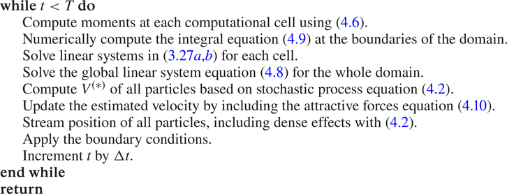
Since the SDEs (3.1a) and (3.1b) do not admit closed-form time integration (due to nonlinearity of the drift), a numerical scheme has to be adopted. As explained by Jenny et al. (Reference Jenny, Torrilhon and Heinz2010), Gorji et al. (Reference Gorji, Torrilhon and Jenny2011), Gorji & Jenny (Reference Gorji and Jenny2014), the simple Euler–Maruyama scheme does not guarantee energy conservation on average. Given the fact that the Langevin equation with linear drift allows for explicit time integration, a decomposition of the SDEs into a linear drift portion and a remainder is pursued.
Following Sadr & Gorji (Reference Sadr and Gorji2017) we consider a spatial discretization where each cell  $c$ contains
 $N_{p,{(\textit {c})}}$ particles. Then the evolution of each particle is described via an explicit time-stepping scheme, where the solution at time step
 $(n+1)$ is computed based on the observables estimated at the
 $(n)$th step.
Realizations of the SDEs (3.1a) and (3.1b), through particles with weights  $w^{(k)}$, velocities
 $V^{(k)}$ and positions
 $X^{(k)}$ with
 $k\in \{1,\ldots ,N_p\}$, provide an estimate
 \begin{equation} \mathcal{F}(v,x,t)\approx \sum_{k=1}^{N_p}w^{(k)} \delta ( V^{(k)}(t)- v)\delta( X^{(k)}(t)- x) \end{equation}
of the distribution which can be used to obtain various observables. By generalizing particle discretization introduced by Gorji & Jenny (Reference Gorji and Jenny2014), the velocity and position of each particle gets updated as
 \begin{equation} V_i^{(*)}= \langle
V_i \rangle^{(n)}_{(\textit{c})} +
\alpha_{(\textit{c})}\tilde{V}^{(n)}_i, \\ X_i^{(n+1)}=
X_i^{(n)} + V_i^{(n+1)}{\rm \Delta} t+\delta \tilde{X}^{(n)}_i,
\end{equation}
where
 \begin{align} \tilde{V}^{(n)}_i&= V_i^{\prime, (n)} \,\textrm{e}^{-{\rm \Delta} tY^{(n)}/\tau^{(n)}} + c^{(n)}_{ij} V_j^{\prime, (n)}+ \gamma^{(n)}_i ( V_j^{\prime, (n)} V_j^{\prime, (n)} - 3k_bT^{(n)}/m ) \nonumber\\ &\quad + \varLambda ( V^{\prime, (n)}_i V^{\prime, (n)}_j V^{\prime, (n)}_j - 2q^{(n)}_i/\rho^{(n)}) + \sqrt{\frac{kT^{(n)}Y^{(n)}}{\tau^{(n)} m}({1-\textrm{e}^{{-2{\rm \Delta} tY^{(n)}}/{ \tau^{(n)}}}})} \xi_i, \end{align}
and
 \begin{align} \delta \tilde{X}^{(n)}_i&= ( \hat{c}^{(n)}_{ij} V^{\prime, (n)}_j + \hat{\gamma}^{(n)}_i (V^{\prime, (n)}_j V^{\prime, (n)}_j - {3k_bT^{(n)}}/{m}) \nonumber\\ &\quad + \hat{\varLambda}^{(n)} ( V^{\prime, (n)}_i V^{\prime, (n)}_j V^{\prime, (n)}_j - 2q^{(n)}_i/\rho^{(n)} ) {\rm \Delta} t. \end{align}
Notice that  $V^{(*)}$ is modified accordingly once external or long-range forces are considered; otherwise, we have
 $V^{(n+1)} = V^{(*)}$. Here
 $\xi _i$ is a random number drawn from the standard normal distribution, i.e.
 $\xi _i \sim \mathcal {N}(0,1)$, and
 $\alpha ^{(\textit {c})}$ is the scaling factor which guarantees conservation of kinetic energy at each cell for a given time step,
 \begin{equation} \alpha_{(\textit{c})} =\frac{\langle V_{j}^{\prime, (n)} V_{j}^{\prime, (n)} \rangle_{(\textit{c})} } {\langle \tilde{V}_j^{(n)} \tilde{V}_{j}^{(n)} \rangle_{(\textit{c})}}.\end{equation}
Note that  $\langle \cdot \rangle ^{(\textit {c})}$ indicates a moment estimator. Using (4.1), we observe that
 \begin{equation} \langle \hat{\phi} \rangle_{(\textit{c})} = \frac{1}{\hat{\rho}} \sum_{i\in \mathcal{S}_c} w^{(i)}{\hat{\phi}}^{(i)},\end{equation}
where  ${\hat {\phi }}^{(i)}$ indicates
 $\phi$ evaluated by the
 $i$th particle,
 $\mathcal {S}_c$ is a set of particles in the cell
 $(\textit {c})$ and
 \begin{equation} \hat{\rho}= \frac{1}{\delta V_c}\sum_{i\in \mathcal{S}_c}w^{(i)} \end{equation}
is the estimated density based on the cell volume  $\delta V_c$.
In comparison to conventional Langevin simulations, here the macroscopic coefficients  $\{ c, \gamma , { \hat {c}}, { \hat {\gamma }}\}$ which close the drift term are computed from linear systems (3.27a,b) for each computational cell and per each time step. Hence, correct relaxation rates in the velocity update besides accurate collisional transfer in the position update are obtained.
DFP-SP solution algorithm

4.2. Discretization of the screened-Poisson model
In order to translate the long-range interactions into a suitable elliptic problem we first need to represent (3.31) in a bounded domain  $\varOmega _x \subset \mathbb {R}^3$. Following uniqueness of the solution, the SP equation can be reset in a bounded domain
 $\varOmega _x$ as
 \begin{equation} \left\{\begin{array}{@{}ll} ({\rm \Delta} -\lambda^2) \tilde{\varPhi}_{r>0} ={-}n & \text{in }\varOmega_x, \\ \tilde{\varPhi}_{r>0} = \tilde{\varPhi}_D & \text{on }\partial \varOmega_x, \end{array}\right.\end{equation}
where the Dirichlet condition  $\tilde {\varPhi }_D$ is evaluated via
 \begin{equation} \tilde{\varPhi}_D(x) = \int_{r>0} G(r) n(y)\, {\textrm{d} y}, \quad \forall\, x\in\partial \varOmega_x. \end{equation}
The boundary term is computed numerically using quadrature estimation of the Vlasov integral and introducing a cut-off to contain the computational cost, i.e.  $r\in (0, r_{{cut}})$. Note that the singularity in
 $G(r)$ is avoided once the integral is formulated in the spherical coordinates. Here, we have set
 $r_{{cut}} = 3 \sigma$ and used
 $N_{{quad}}$ Legendre–Gauss quadrature points for the numerical integration. Once the values of the unique global solution on the boundary
 $\partial \varOmega _x$ is computed, this elliptic differential equation on the bounded domains can be solved for the interior of the domain using standard numerical methods. In Appendix B we present a short description for the adopted hybridized discontinuous Galerkin solver. Once our estimate of the attractive force at time step
 $(n)$ is obtained, the velocity update takes the form
 \begin{equation} V^{(n+1)}= V^{(*)}+\hat{H}^{(n)}(X^{(n)}){\rm \Delta} t,\end{equation}
where  $\hat {H}^{(n)}(X^{(n)})$ is the approximated attractive force at the particle position
 $X^{(n)}$ (see Appendix B for details).
4.3. Solution algorithm
It is evident from the time-stepping scheme given by (4.2a) and (4.2b) that the evolution of the position and velocity of particles is decoupled during each time step. While more accurate schemes such as those discussed by Jenny et al. (Reference Jenny, Torrilhon and Heinz2010), Gorji et al. (Reference Gorji, Torrilhon and Jenny2011), Jenny & Gorji (Reference Jenny and Gorji2019) can be devised for a joint position-velocity update, here for simplicity, the decoupled version is utilized. Note that, as shown by Pfeiffer & Gorji (Reference Pfeiffer and Gorji2017), Jun et al. (Reference Jun, Pfeiffer, Mieussens and Gorji2019), this decoupling is accurate and justified as long as the gradients of macroscopic fields are resolved. In comparison to DSMC (Bird Reference Bird1994), where the collisional scales have to be resolved, here we obtain a significant computational advantage by relaxing the discretization constraints.
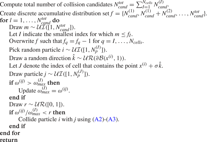
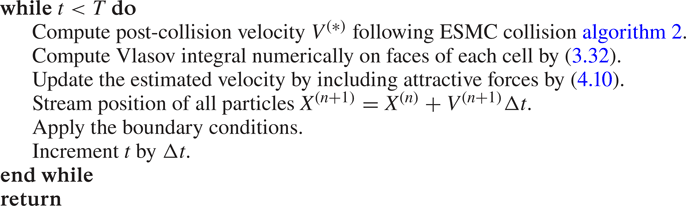
Algorithm 1 provides a summary of the DFP-SP solution method for simulations of multi-phase flows. Prior to the simulation, the domain is discretized into a set of computational cells. Furthermore, an appropriate time step size and particle weight are chosen. After initializing the particles according to their weights and initial density field, the particles evolve according to algorithm 1. Note that the particles boundary conditions are implemented similar to DSMC, where depending on the distribution of incoming or reflected particles, open or wall boundaries are handled, respectively.
5. Validation results
For validation of the devised DFP-SP solution algorithm, we focus on evaporation of a liquid argon slab once in contact with the equilibrium vapour and once in contact with the vacuum. The coefficients of the Sutherland potential  $\phi (r)$ are chosen according to
 $\sigma =3.405\times 10^{-10}\ \mathrm {m}$ and
 $\phi _0=4.17 \epsilon$, where
 $\epsilon = 119.8 k_b\ {\rm kg}\cdot {\rm m}^2\cdot {\rm s}^{-2}$ (Rowley, Nicholson & Parsonage Reference Rowley, Nicholson and Parsonage1975). Fitting
 $\tilde {\phi }(r)$ to the attractive part of the Sutherland potential leads to the coefficients
 $a=-1.64835851\times 10^{-28}\ {\rm kg}\cdot {\rm m}^2\cdot {\rm s}^{-2}$ and
 $\lambda =6.91304716\times 10^{9}\ \mathrm {m}^{-1}$.
We examine accuracy of the DFP-SP model in predicting capillary properties of droplets, such as the surface tension and the evaporation rate. The results are then compared with benchmark Monte-Carlo simulations of the EV equation (ESMC-Vlasov). For implementation details of the benchmark ESMC-Vlasov approach, see Appendix A.
The time step size satisfying a Courant–Friedrichs–Lewy (CFL) type condition
 \begin{gather} {\rm \Delta} t \leq \frac{min(\lambda^{(0)}, h)}{max( \sqrt{k T^{(0)}/m})}, \end{gather}
 \begin{gather}\textrm{where} \quad \lambda^{(0)} = \frac{1}{\sqrt{2}{\rm \pi}\sigma^2n^{(0)} Y(n^{(0)})}, \end{gather}
is chosen. Here,  $\lambda$ provides an estimate of the mean free path,
 $h$ indicates the mesh size and superscript
 $(\cdot )^{(0)}$ denotes the local initial value. For further details, see Pfeiffer & Gorji (Reference Pfeiffer and Gorji2017).
5.1. Isothermal co-existing states
In this section we investigate the accuracy of the DFP-SP model in predicting the co-existing liquid–vapour states at constant temperatures against ESMC-Vlasov simulation results, besides the Maxwell area reconstruction solution (Li, Luo & Li Reference Li, Luo and Li2013). We impose a thermostat every  $N_{therm}$ steps until the solution reaches stationary state, in order to keep the temperature of the system constant (Frezzotti et al. Reference Frezzotti, Gibelli and Lorenzani2005). The thermostat is then removed and afterwards the system reaches the equilibrium. The thermostat phase provides us with a decent initial distribution of particles in physical space for a given temperature. Furthermore, note that the solution after the thermostat phase is already very close to the steady-state equilibrium solution.
In order to achieve simulation results of co-existing states, we consider a liquid slab  $[0,1] \times [0,40\sigma ] \times [0,1]\ \mathrm {m}^3$ with number density
 $n_l^{(0)}$ inside vapour with number density
 $n_v^{(0)}$. Here, the total volume
 $[0,1] \times [0,L] \times [0,1]\ \mathrm {m}^3$, with
 $L=100 \sigma$, is enclosed in a box with specular walls. Due to symmetry of the solution space, we only need to simulate the particle motion in the
 $x_2$ direction, yet velocity is treated in three-dimensional space. The spatial dimension is decomposed to
 $100$ cells and
 ${\rm \Delta} t$ was chosen to satisfy a CFL number of
 $0.01$. Initially, in each cell
 $N_{p/c}$ particles per cell with a Gaussian distribution in velocities, i.e.
 $V_i \sim \mathcal {N}(v_i|0,3k_bT^{(0)}/m)$, and a uniform distribution in position are sampled. The statistical weight of particles
 $w$ was taken constant and chosen such that
 $N_{p/c}\geq 300$ in the vapour phase. The velocity of particles are thermostated every
 $N_{therm}=10$ steps for the first
 $1000$ steps. Then, the simulation is continued without the thermostat until the stationary state is achieved (
 $\sim 2000$ steps). Then, the solution over next
 $3000$ steps is averaged for the post-processing.
Note that the Maxwell solution leads to a minimization problem, i.e. find the pressure  $p_0 = {\operatorname {argmin}} ( \int _{n_v}^{n_l} p(n,T)-p_0\, \textrm {d} n)$ for a given temperature. This pressure leads to two equal separated areas enclosed between
 $p(n,T)$ and the constant
 $p(n_l,T)=p(n_v,T)=p_0$. In order to compute the integral, one needs to find
 $n_l$ and
 $n_v$ for any guessed pressure
 $p_0$ which leads to finding roots of a nonlinear equation
 $p(n,T)=p_0$ for
 $n$. In order to simplify computation of the Maxwell solution, we approximate the pair correlation function with a polynomial
 $Y(n)\approx 1 + 0.625n b + 0.2869 (n b)^2 + 0.115 (n b)^3+\cdots$, instead of (2.6); see Chapman & Cowling (Reference Chapman and Cowling1970). As shown in figure 1, the polynomial approximation has a reasonable accuracy for the range of
 $n \sigma ^3\leq 0.45$. Hence, we consider the equilibrium pressure
 \begin{gather} p_{eq}^{Max., Suth.} = nk_bT(1+nb\tilde{Y}(n)) - \frac{4 {\rm \pi}}{3} \phi_0 \sigma^2 n^2, \end{gather}
 \begin{gather}p_{eq}^{Max., SP} = nk_bT(1+nb\tilde{Y}(n)) + {a}\, {\textrm{e}^{-\lambda \sigma} } (\lambda^2 \sigma^2 + 3 \sigma \lambda +3 ) n^2/(6 \lambda^2), \quad \mathrm{where} \end{gather}
 \begin{gather}\tilde{Y}(n) = 1 + 0.625n b + 0.2869 (n b)^2 + 0.115 (n b)^3, \end{gather}
for the Maxwell area reconstruction solution of co-existing states with validity range of  $0< n \sigma ^3\leq 0.45$.
Pair correlation function  $Y(n)$ and polynomial approximation
 $\tilde {Y}(n)$ used in the Maxwell solution against normalized density for
 $n\sigma ^3\in (0,0.6)$.

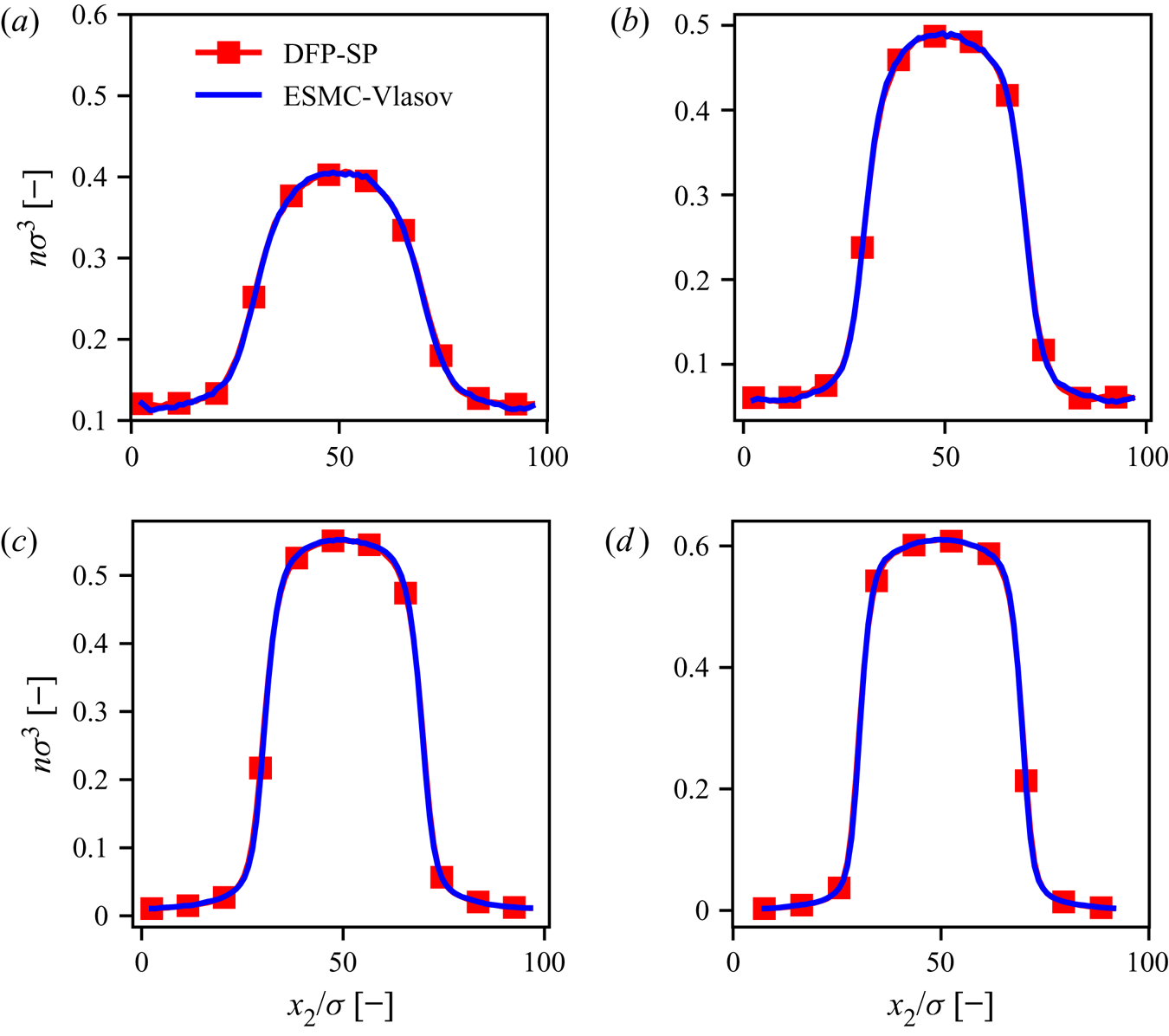
Here, we consider several equilibrium states within  $T \in [130,185]\ \mathrm {K}$. The initial number density of vapour and liquid for each case is provided in table 1. The density and temperature profiles for each case are shown in figures 2–4, respectively, where a reasonable consistency between DFP-SP and ESMC-Vlasov solutions is observed. The obtained
 $(n,T)$ pair for liquid and vapour of each case is plotted against the Maxwell area reconstruction solution in figure 5, where a reasonable agreement between the kinetic solution and Maxwell area reconstruction can be seen for its range of validity.
Initial number density and temperature of liquid slab and vapour for the co-existing state simulations.

Number density profiles for simulation of the DFP-SP model (in red) and ESMC-Vlasov solution algorithm (in blue) for the obtained isothermal equilibrium simulation in (a)  $T = 180\ \mathrm {K}$, (b)
 $T = 170\ \mathrm {K}$, (c)
 $T = 160\ \mathrm {K}$ and (d)
 $T = 150\ \mathrm {K}$.

Number density profiles for simulation of the DFP-SP model (in red) and ESMC-Vlasov solution algorithm (in blue) for the obtained isothermal equilibrium simulation with (a)  $T=140\ \mathrm {K}$, (b)
 $T=140\ \mathrm {K}$, log-scale, (c)
 $T=130\ \mathrm {K}$ and (d)
 $T=130\ \mathrm {K}$, log-scale.

Temperature profiles obtained from simulation of the DFP-SP model (a) and ESMC-Vlasov solution algorithm (b) for co-existing state test case at temperatures  $T\in \{130, 140,150,160,165,170,175,180,185\}\ \mathrm {K}$ shown in rainbow spectrum, from dark blue to red.

5.2. Evaporation near equilibrium
In order to present the DFP-SP prediction of the surface tension, evaporation of a liquid argon slab in contact with the vapour phase near equilibrium is studied. In particular, we consider the phase transition of the liquid slab located within  $[0,1]\times [0,30 \sigma ] \times [0,1]\ \textrm {m}^3$ which is surrounded by the vapour confined in
 $[0,1]\times [0,L] \times [0,1]\ \textrm {m}^3$, with
 $L=90 \sigma$. Since only the
 $x_2$ direction is relevant, the other dimensions in the physical space are ignored in the evolution of particles positions. The liquid slab and the vapour around it are initialized with number densities
 $n_{{liq}}$ and
 $n_{{vap}}$, respectively. In order to maintain the stationary scenario, the liquid slab is heated up every
 $N_{{therm}}$ steps, where the particles inside
 $x_2\in [L/2-L_{{therm}}/2,L/2+L_{{therm}}/2]$ are thermostated with the initial temperature
 $T^{(0)}$. This is achieved by rescaling the particles fluctuating velocities. Furthermore, the specular reflection boundary conditions are deployed here.
After conducting convergence studies, it is found that  $N_{{cell}}=180$ computational cells and the CFL number
 $0.01$ provide converged results. Moreover, a fixed statistical weight of
 $w=10^{14}$ was picked for the test cases with
 $T^{(0)} \in \{150, 160, 170, 180 \}\ \mathrm {K}$,
 $n_{{liq}}^{(0)}\in \{0.6,0.526,0.45,0.36 \} \times \sigma ^{-3} \ \mathrm {m}^{-3}$ and
 $n_{{vap}}^{(0)} \in \{ 0.05,0.077,0.12,0.15 \} \times \sigma ^{-3} \ \mathrm {m}^{-3}$. The stationary distribution is obtained after
 $5000$ steps and the time averaging is performed over
 $15\,000$ steps onward. Here,
 $L_{{therm}}=10 \sigma$ was chosen as the length of the thermostated sub-domain which was carried out once every
 $N_{{therm}}=1000$ steps. The initial densities of vapour and liquids for each simulation were picked such that unstable regions of the phase diagram are not met, as depicted in figure 6. Here, the total equilibrium pressure is
 $p_{{eq}}^{{tot}}(n,T) :=nk_bT(1+nbY)+p^{{att}}$, where the attractive part
 \begin{equation} p^{att}_{{eq}}(n)={-}({2{\rm \pi} }/{3})n^2 \int_0^\infty r^3 \frac{\partial \phi(r)}{\partial r} \, \textrm{d} r \end{equation}
becomes  $p^{att}_{{eq}}(n)=-({4 {\rm \pi}}/{3}) \phi _0 \sigma ^3 n^2$ and
 $p^{{att}}_{{eq}} (n) = {a } { \textrm {e}^{-\lambda \sigma } } (\lambda ^2 \sigma ^2 + 3 \sigma \lambda +3 ) n^2/(6 \lambda ^2)$ in the case of Sutherland and screened-Poisson potentials, respectively (Sadr & Gorji Reference Sadr and Gorji2019).
For the liquid slab at equilibrium, the surface tension coefficient  $\gamma$ is defined as a norm of the difference between the diagonal element of the kinetic pressure tensor and the equilibrium kinetic pressure across the phase transition,
 \begin{equation} \gamma = \tfrac{1}{2} \int_0^L (p_{22}-p_0) \, \textrm{d} x_2. \end{equation}
For details, see Ghoufi & Malfreyt (Reference Ghoufi and Malfreyt2010) and Hirschfelder et al. (Reference Hirschfelder, Bird and Curtiss1964). The integration over the domain can be taken numerically, since the discrete values of the pressure tensor are estimated at every cell.
Comparison between simulation results obtained from the DFP-SP model with respect to the benchmark ESMC-Vlasov is shown in figure 7. Although the DFP-SP model underpredicts the peak in estimating  $|p_{22}-p_0|$ at the interface, overall a very good agreement between the two is observed. Note that the discrepancy in
 $\gamma$ between both methods increases as the liquid gets denser at lower temperatures. Furthermore, the computational costs of the discussed simulation settings are presented in figure 8. Accurate quantification of the relative computational costs would require a well-designed prospective study with detailed numerical investigations. However, a general comparison is possible by comparing the complexity order of ESMC-Vlasov and DFP-SP methods. For the former, observe that the number of operations follows
 $\mathcal {O}(n\sqrt {T})$. Yet the cost of the latter is independent of the density, which makes our assembled approach attractive for efficient Monte-Carlo simulations of multi-phase flows.
Co-existing states obtained from simulations of the DFP-SP model (in red), ESMC-Vlasov solution algorithm (in blue), and Maxwell area reconstruction solution of Sutherland (in black) and screened-Poisson potential (in green) for equilibrium at  $T\in \{130, 140,150,160,165,170,175,180,185\} \ \mathrm {K}$ with relative error in density of vapour
 $|n_v^{DFP-SP}-n_v^{ESMC-Vlasov}|/n_v^{ESMC-Vlasov}={0.052, 0.037,0.002,0.004,0.06,0.039,0.001,0.05,0.01}$, respectively. Density for the Monte Carlo solution is obtained by averaging over cells within
 $x_2\in (0,5\sigma )\cup (L-5\sigma ,L)$ and
 $x_2\in (L/2-5\sigma , L/2+5\sigma )$ for vapour and liquid, respectively. (a) Co-existing states for
 $n_l \sigma ^3\leq 0.55$ in log-scale and (b) co-existing states extended.

Contours of total equilibrium pressure  $p_{{eq}}^{{tot}}(n,T){:=nk_bT(1+nbY)+p^{{att}}_{{eq}}}$ at constant temperatures as well as the initial state pairs
 $(n_{{liq}},T_{{liq}})$ and
 $(n_{{vap}},T_{{vap}})$ for the evaporation test case with initial temperatures of
 $T^{(0)}\in \{ 150,160,170,180 \} \ \mathrm {K}$ and corresponding vapour (in red) and liquid (in blue) number densities of
 $n_{{liq}}^{(0)}=\{0.6,0.526,0.45,0.36 \} \times \sigma ^{-3} \ \mathrm {m}^{-3}$ and
 $n_{{vap}}^{(0)}=\{ 0.05,0.077,0.12,0.15 \} \times \sigma ^{-3} \ \mathrm {m}^{-3}$, respectively. Note that here the total pressure with attractive part associated with screen-Poisson's potential is used,
 $p^{att}_{{eq}}(n)={{a } { \textrm {e}^{-\lambda \sigma } } (\lambda ^2 \sigma ^2 + 3 \sigma \lambda +3 ) n^2/(6 \lambda ^2)}$.

Phase transition of argon at  $T^{(0)}=160\ \mathrm {K}$. (a) Normalized number density. (b) Normalized temperature. (c) Normalized difference between diagonal and equilibrium kinetic pressure. (d) Normalized surface tension for liquid temperatures of
 $T^{(0)}\in \{ 150,160, 170, 180 \}\ \mathrm {K}$. Here, a maximum relative error of 7% in evaluating
 $\gamma$ is observed.

Execution time per particle  $\tau :=t^{{ex.}}/N_p$ for evaporation simulation at the equilibrium using ESMC-Vlasov and DFP-SP solution algorithms. The cost is normalized by
 $\tau _0$ denoting DFP-SP execution time for the case
 $T^{(0)}=180$ K.

Next, we compare the obtained numerical results in estimating the surface tension coefficient with respect to an analytical approximation based on the free surface energy  $S(T)$. Following Elsner (Reference Elsner1991),
 \begin{equation} \gamma(T) = T \int_T^{T_{crit}} \frac{S(T)}{T^2} \, \textrm{d} T, \end{equation}
where
 \begin{equation} S(T) = \frac{\alpha}{3} \int_{\vartheta _v}^{\vartheta _l} \left(\frac{\mu}{\vartheta }-p_v\right)\frac{\textrm{d} \vartheta }{\vartheta^{2/3}}. \end{equation}
Here,  $\vartheta =1/n$ denotes the reciprocal number density,
 $\mu$ is the chemical potential,
 $p_v$ is the vapour pressure and
 $\alpha$ a proportionality factor. Note that
 $\mu -p_v \vartheta$ gives the Helmholtz free energy per particle. For simplicity, similar to Hadjiconstantinou et al. (Reference Hadjiconstantinou, Garcia and Alder2000), we set
 $\alpha =0.6$ (for all temperatures). Furthermore, we calculate the chemical potential through
 \begin{equation} \frac{\mu}{T} = \frac{\mu_{crit.}}{T_{crit.}} - \int_{p_v/T}^{p_v/T} \vartheta \, \textrm{d} (p_v/T), \end{equation}
where
 \begin{gather} \frac{\mu_{crit.}}{T_{crit.}} ={-} k_b (2\xi_{crit.} + \ln(\vartheta _{crit.}/\vartheta _{q,\textit{crit.}})), \end{gather}
 \begin{gather}\xi_c = \frac{\vartheta _{crit.} p_{crit.}}{k_b T_{crit.}}, \end{gather}
 \begin{gather}\textrm{and} \quad \vartheta _{q} = \frac{\hbar^3}{(2{\rm \pi} m k_b T)^{3/2}}. \end{gather}
Note that  $\hbar$ is the Planck constant (see Elsner (Reference Elsner1989) for details). Figure 7(d) shows reasonable agreement between all three considered methods, i.e. analytical Elsner's approach, the DFP-SP model and the ESMC-Vlasov simulation results.
5.3. Evaporation to vacuum
Since streaming of the stochastic particle in the DFP model is consistent with the Enskog equation only on the moment level, the measurement of evaporation rate based on particle trajectory as suggested in Yasuoka, Matsumoto & Kataoka (Reference Yasuoka, Matsumoto and Kataoka1994), Kon et al. (Reference Kon, Kobayashi and Watanabe2014), Kobayashi et al. (Reference Kobayashi, Hori, Kon, Sasaki and Watanabe2016) would not lead to an accurate estimation of the desired property. Alternatively, the evaporation rates can be approximated via moments as a liquid slab evaporates into the vacuum; see Frezzotti et al. (Reference Frezzotti, Gibelli and Lorenzani2005). The outflow mass flux  $\dot {m}_{{out}}$ is indeed a function of the evaporation rate
 $\sigma _e$,
 \begin{equation} \dot{m}_{{out}} =A \sigma_e n_g(T_L) \sqrt{\frac{k_b T_L}{2 {\rm \pi}m}}, \end{equation}
where  $A$ indicates the area of cross-section normal to the interphase,
 $n_g(T_L)$ is the number density of the gas computed at the temperature of the liquid phase
 $T_L$. Hence, validation for the evaporation rate translates into the consistency of temperature and density profiles, as well as the outgoing mass flux with respect to the benchmark solution. Except for the boundary conditions, we consider similar simulation settings as the test case with the evaporation of liquid at equilibrium, i.e. § 5.2. Particles are reinitialized in the liquid slab as they leave the domain with the new position sampled randomly from a uniform distribution on the interval
 $x_2\in [L/2-L_{{therm}}/2,L/2+L_{{therm}}/2]$. For the reinitialized particle, the velocity component in the relevant flow direction, i.e.
 $V_2$, is sampled again from an equilibrium distribution with mean and temperature of the local computational cell, as the other components of the velocity remain unchanged.
In comparison to ESMC-Vlasov, we obtain accurate predictions of temperature, density, velocity and the outflow mass flux, as shown in figure 9. Similar test cases were performed at other temperatures and again good agreements between the DFP-SP model and the benchmark were observed, indicating consistent evaporation rates.
Simulation results for evaporation of liquid argon into the vacuum obtained from ESMC-Vlasov and DFP-SP models. (a) Normalized number density. (b) Temperature. (c) Mean velocity. (d) Outflow mass flux.

6. Inverted temperature gradient
One ofthe interesting examples where counterintuitive non-equilibrium effects become evident is the inverted temperature profile in the vapour phase contained between two liquid slabs at different temperatures. First, Pao (Reference Pao1971) found out that the temperature profile does not increase monotonically from a cold to hot liquid, suggesting an inverted temperature profile in the vapour phase. Since then, this phenomenon has been studied and validated in detail using tools across MD and kinetic theory (see, e.g Frezzotti, Grosfils & Toxvaerd Reference Frezzotti, Grosfils and Toxvaerd2003; Meland Reference Meland2003; Meland & Ytrehus Reference Meland and Ytrehus2004).
We tackle this problem by the devised DFP-SP model, and validate our results with respect to the ESMC-Vlasov approach. Consider a solution domain in the physical space  $\varOmega =[0,1]\times [0,L]\times [0,1]\ \mathrm {m}^3$, where
 $L=70 \sigma$. Cold and hot liquid slabs are located at
 $x_2\in [0,L_c]$ and
 $x_2\in [L-L_h,L]$, respectively, with
 $L_c=L_h=15 \sigma$. The thermodynamic states of cold and hot slabs are initially set by the density–temperature pairs
 $(n_c,T_c)$ and
 $(n_h,T_h)$, respectively. The vapour with initial density–temperature of
 $(n_v,T_v)$ fills the space between two slabs as depicted schematically in figure 10. In order to keep temperature of the liquid slabs close to the initial setting, particles within
 $x_2\in [0,L_{{therm}}]$ and
 $x_2\in [L-L_{{therm}}, L]$, where
 $L_{{therm}}=15 \sigma$, are thermostated to the initial temperature every
 $N_{{therm}}$ steps. This is done by rescaling particles fluctuating velocities. Due to symmetry of the simulation setting, position evolution of the particles is considered only along the
 $x_2$-coordinate.
Schematic of the inverted temperature gradient simulation.

Fully diffusive scattering is applied as the boundary condition to both ends of the domain. As particles leave the domain, their velocities are sampled from the flux of the Maxwellian distribution with the initial temperature of the nearest liquid slab. Next the scattered particles are streamed into the domain for the remaining fraction of the time step.
Since there exists a mass flux from hot slab towards to the cold one, the system does not admit a stationary state. Hence, time averaging can not be deployed to improve the estimate of observables. However, by moving the observer in the direction opposite to the mass flux, a quasi-stationary condition is reached where time averaging becomes applicable. Notice that a similar approach is typically utilized for one-dimensional shock wave problems (Bird Reference Bird1994; Gorji & Jenny Reference Gorji and Jenny2013). Once every  $N_{{shift}}$ steps, the simulation frame is moved by
 ${\rm \Delta} /2$, where
 ${\rm \Delta} :=(\mathcal {V}_c-\mathcal {V}_h)$,
 $\mathcal {V}_c:=x_L$ and
 $\mathcal {V}_h:=(L-x_R)$. Here
 $x_R$ is the rightmost location with number density
 $0.9n_h$, whereas
 $x_L$ is the leftmost position with number density
 $0.9n_c$. As the simulation frame is moved, the particles which appear outside of the domain are removed. Moreover, new particles are generated to fill the void space. Velocities of the newly introduced ones are sampled from the Maxwellian distribution with temperature of the nearest liquid slab. Their corresponding positions are sampled uniformly inside the void space.
Three settings with temperatures below the critical point are considered, as presented in table 2. The temperature difference between liquid slabs is set to  $2\ \mathrm {K}$. After a convergence study, a uniform discretization of physical space with a mesh size of
 ${\rm \Delta} x_2=\sigma /2$ along the
 $x_2$ direction as well as the CFL number
 $0.01$ are picked due to their reasonable accuracy. In all simulations initially
 $10\ 000$ particles per cell for the vapour phase are generated, leading to the statistical weights
 $w \in \{4.3, 5.1,5.6 \} \times 10^{13}$ associated with cold liquid slab temperatures
 $T_{c} \in \{ 165,167,170 \}\ \mathrm {K}$, respectively. Furthermore, the domain is shifted every
 $N_{{shift}}=500$ steps and the liquid slabs are thermostated every
 $N_{{therm}}=1000$ steps, for all considered cases. As depicted in figure 12, the DFP-SP solution algorithm approximates the density, the mean velocity, the temperature and the heat flux of the considered test cases accurately in comparison to the benchmark. The inverted temperature gradients are well recovered by the presented DFP-SP model. Furthermore, the profiles near the phase transition regimes are found to be well approximated. As suggested by Meland & Ytrehus (Reference Meland and Ytrehus2004), since the colder liquid slab has smaller evaporation and condensation rates, we observe an accumulation of hot particles near the colder liquid slab. This leads to the conclusion that particles emitted from the hot liquid slab play a more important role behind this counterintuitive non-equilibrium temperature profile.
Initial number density and temperature of liquid slabs and the vapour for the inverted temperature gradient simulations.

In order to obtain a better understanding of the underlying phase transition dynamics, let us consider the case where a single liquid slab distributed in  $x_2 \in [0,10\sigma ]$ is in contact with a diffusive wall at
 $x_2=0$ and is surrounded by the vapour distributed inside
 $x_2 \in [10\sigma ,20\sigma ]$. For simplicity, we consider the specular wall at the end of domain
 $x_2=20 \sigma$ to contain the vapour. We simulated this setting using the DFP-SP model for liquid temperatures considered in the inverted temperature gradient test case using
 $\omega =4\times 10^{13}$, CFL number
 $0.01$ and
 ${\rm \Delta} x = \sigma /2$. As shown in figure 11, the temperature of the fluid first drops during the transition of the liquid to the vapour and then raises back inside the vapour phase. It is important to notice that the further we move far from the droplet, the more increase we observe in the temperature. This can be explained by noting that at relatively low vapour pressure, high energy particles can travel longer distances before reaching equilibrium with the background gas. Here, one can make three observations. First, note that as the temperature of the liquid decreases, the difference between temperature of the liquid and its surrounding vapour becomes larger. Next, the temperature drop gets more pronounced, once colder liquid slabs are considered. Finally, by a simple superposition of the observed single liquid slab temperature profiles, we get a qualitative picture of the inverted temperature gradient behaviour consistent with our two liquid slabs system shown in figure 12.
Single droplet evaporation. The profile of number density, temperature and heat flux for the liquid/vapour contained between diffusive and specular walls. (a) Number density, (b) temperature and (c) heat flux.

Normalized number density, mean velocity, temperature and heat flux obtained from inverted temperature gradient simulations using ESMC-Vlasov (blue) and DFP-SP (red) solution algorithms. The critical point  $(n_{{crit.}},T_{{crit.}})=(0.3568/\sigma ^3 \ \mathrm {m}^{-3},188.33\ \mathrm {K})$ is used to normalize density and temperature. Heat flux and mean velocity are normalized by
 $\hat {q}_2:=q_2/(\rho _c (kT_c/m)^{3/2})$ and
 $\hat {U}_2:=U_2/\sqrt {kT_c/m}$, respectively. (a) Test case (I), (b) test case (II) and (c) test case (III).

7. Spinodal decomposition
Phase transition phenomena which are pronounced in breakup and coalescence of bubbles as well as droplets, comprise one of the grand challenges in simulation of multi-phase flows. In particular, an accurate description of these processes demands incorporation of mass, momentum and energy transfer among different phases, if conventional multi-phase solvers are considered (Shan & Chen Reference Shan and Chen1993; Watanabe, Ito & Hu Reference Watanabe, Ito and Hu2012). However, due to the fact that the considered EV kinetic framework provides a universal flow description across liquid and gas phases, a systematic exchange of mass, momentum and energy at the interface is obtained naturally, consistent with the underlying molecular potential. In order to demonstrate the potential of the devised kinetic model in simulating such scenarios, here we study the spinodal decomposition of argon, where the formation of droplets as well as bubbles can be investigated.
Let us consider a simulation domain  $\varOmega _x=[0,L]^2\times [0,1]\ \mathrm {m}^3$, where
 $L=5\times 10^{-8}\ \mathrm {m}$. Furthermore, assuming symmetry in the third dimension, we intend to study a two-dimensional planar fluid flow in
 $\varOmega _x$ that, after a convergence study, is discretized with
 $250\times 250\times 1$ cells. As boundary conditions for relevant dimensions, i.e.
 $x_1$ and
 $x_2$, we consider specular reflection for particles that leave the domain. This leads to the Neumann boundary condition for the SP model owing to long-range interaction, i.e.
 $\tilde {n}_i \partial \tilde {\varPhi }/\partial x_i = 0$, where
 $\tilde {n}$ indicates the unit outward normal vector on the surface of the boundary
 $\partial \varOmega _x$.
First, particles are initialized inside the domain  $\varOmega _x$ with a uniform distribution in physical space and Maxwellian in velocity for a given initial number density
 $n^{(0)}$ and temperature
 $T^{(0)}$. The idea is to pick an unstable state
 $(n^{(0)},T^{(0)})$ from a point on the phase diagram that does not belong to liquid nor vapour at the equilibrium. Then, we let the system relax towards the equilibrium. The expectation is that particles move away from this unstable initial condition until the corresponding mixture reaches a stable state at the equilibrium on the binodal diagram. Here we considered three test cases, as detailed in table 3, with the main difference in their initial densities. The intention behind these cases is to study the formation of droplets in a (A) low density range and (B) medium density range. Furthermore, the formation of bubbles is tackled in a high density range test case (C).
Simulation setting of the spinodal decomposition. Initial number density  $n^{(0)}$, temperature
 $T^{(0)}$, the time step size
 ${\rm \Delta} t$ and number of particles
 $N_p$ used in the simulations are reported here.

Test case (A): formation of nano droplets
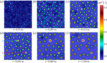
As shown in supplementary movie 1, which is available at https://doi.org/10.1017/jfm.2021.461 and depicted in figure 13, the formation and coalescence of droplets can be observed following the evolution of the number density. Note that two droplets, designated by rings around them and identified in the figure, are tracked in time for further analysis.
Evolution of normalized number density in the spinodal decomposition of argon obtained from simulation results of the DFP-SP model for test case (A), with initial number density  $n^{(0)}=3\times 10^{27}\ \mathrm {m}^{-3}$ and temperature
 $T^{(0)}= 120\ \mathrm {K}$ in the domain
 $\varOmega _x=[0,L]^2\times [0,1]\ \mathrm {m}^3$, where
 $L=5\times 10^{-8}\ \mathrm {m}$. Here, two droplets are labelled with rings around them which are tracked in time for further analysis.

As shown in figure 14, unless interrupted by a merge with another droplet, the radius of both droplets first increases with the rate of  $t^{1/3}$ and then their growth rate reduces to
 $t$. At the first stage, when the inertia of the fluid system is negligible, the Lifshitz–Slyozov mechanism is dominant (Siggia Reference Siggia1979). This mechanism gives the growth rate of
 $t^{1/3}$ consistent with our result. Next, once we reach critical quenches (similar volume fraction of both phases), the growth rate stabilizes at the growth rate of
 $t$ (Siggia Reference Siggia1979; Bastea & Lebowitz Reference Bastea and Lebowitz1997).
Growth of the labelled droplets, i.e. droplet  $\#$1 in (a) and
 $\#$2 in (b) as identified in figure 13, are studied by investigating the evolution of droplet's radius
 $r$ in time. We observe that the initial growth of radius in both cases is
 $\propto t^{1/3}$ which follows by
 $\propto t$ unless interrupted by a coalescence, e.g. in (b).

Furthermore, statistics of number density, temperature and velocity magnitude is shown in figures 15 and 16(a). Moreover, we study the total energy of the system
 \begin{equation} E_{{total}}(t)= \underbrace{\frac{1}{2}\int_{\varOmega_x} \rho(x,t) \mathbb{E}[V_j V_j|x,t]\, {\textrm{d} x}}_{E_{{kin}}(t)} + \underbrace{\frac{1}{2m} \int_{\varOmega_x} \rho(x,t) \tilde{\varPhi}(x,t)\, {\textrm{d} x} }_{E_{{pot}}(t)}, \end{equation}
as derived in Appendix C, and here is evaluated numerically from the simulation results. As shown in figure 16(b), we observe energy transformation from potential to kinetic at the early stage of the spinodal decomposition, while the total energy stays almost constant. Furthermore, we observe a relatively small decay of the total energy of the system, which is due to numerical errors in the deployed time integration scheme.
Evolution of maximum, minimum, median and average values of normalized number density as well as temperature in the whole simulation domain for test case (A). Results are obtained using the DFP-SP model.

Evolution of maximum, minimum, median and average values of velocity magnitude in the whole simulation domain for test case (A) shown in (a). The evolution of kinetic, potential and total energy of the system are depicted in (b). Here,  $[\mathrm {a}]$ denotes the prefix unit called atto, where
 $\mathrm {a}=10^{-18}$. Results are obtained using the DFP-SP model.

Test case (B): formation of larger droplets
Since here the initial unstable state has a larger density with respect to case (A), more sizable droplets are formed as illustrated in the evolution of the number density in supplementary movie 2 and figure 17. The maximum, median and minimum values of number density, temperature, velocity magnitude as well as kinetic, potential and total energy are computed. The results are shown in figures 18 and 19(b). Unlike test case (A), we observe the appearance of more nano droplets in the early stage of the spinodal decomposition, which leads to the subsequent formation of larger droplets as coalescence among more nano droplets occurs.
Evolution of normalized number density in the spinodal decomposition of argon obtained from simulation results of the DFP-SP model for test case (B), with initial number density  $n^{(0)}=5\times 10^{27}\ \mathrm {m}^{-3}$ and temperature
 $T^{(0)}= 120\ \mathrm {K}$ in the domain
 $\varOmega _x=[0,L]^2\times [0,1]\ \mathrm {m}^3$, where
 $L=5\times 10^{-8}\ \mathrm {m}$.

Evolution of maximum, minimum, median and average values of normalized number density as well as temperature in the whole simulation domain  $\varOmega _x$ for spinodal decomposition of argon with settings of case (B). Results are obtained using the DFP-SP model.

Evolution of maximum, minimum, median and average values of velocity magnitude in the whole domain  $\varOmega _x$ for test case (B) in simulating the spinodal decomposition using the DFP-SP model are shown in (a). The evolution of kinetic, potential and total energy of the system are depicted in (b).

Test case (C): formation of nano bubbles
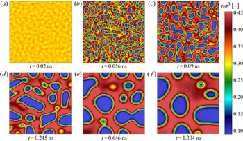
Having initialized spinodal decomposition with a large enough density, here we observe the formation of bubbles instead of droplets, as illustrated in the evolution of the number density in supplementary movie 3 and figure 20. Similar to the last two test cases, statistical investigation of number density, temperature, velocity magnitude as well as kinetic, potential and total energy are shown in figures 21 and 22(b).
Evolution of normalized number density in the spinodal decomposition of argon obtained from simulation results of the DFP-SP model for test case (C), with initial number density  $n^{(0)}=8\times 10^{27}\ \mathrm {m}^{-3}$ and temperature
 $T^{(0)}= 120\ \mathrm {K}$ in the domain
 $\varOmega _x=[0,L]^2\times [0,1]\ \mathrm {m}^3$, where
 $L=5\times 10^{-8}\ \mathrm {m}$.

Evolution of maximum, minimum, median and average values of normalized number density as well as temperature in the whole simulation domain  $\varOmega _x$ for spinodal decomposition of argon with settings of case (C). Results are obtained using the DFP-SP model.

Evolution of maximum, minimum, median and average values of velocity magnitude in the whole domain  $\varOmega _x$ for test case (C) in simulating spinodal decomposition using the DFP-SP model are shown in (a). The evolution of kinetic, potential and total energy of the system are depicted in (b).

Computational cost: As expected, the computational cost of DFP-SP simulations remains identical, as the deployed spatial discretization as well as particle numbers among considered spinodal decomposition test cases are similar. However, once the liquid is formed, the average execution time per  $100$ iterations ranges from
 $360~\mathrm {s}$ to
 $540~\mathrm {s}$, which can be explained by the inhomogeneity of the load balance as particles cluster inside the liquid phase. Note that here the parallelization is based on a domain decomposition of the physical space. For the simulations of the spinodal decomposition, we deployed
 $40$ cores of Intel(R) Xeon(R) Platinum
 $8160$ CPU @
 $2.10$ GHz in parallel. Using this computational resource, the total computation time, e.g. for case (C), with an end time of
 $t_{final}\approx 1.3\ \mathrm {ns}$ was about
 $4$ days.
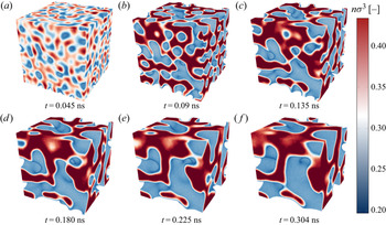
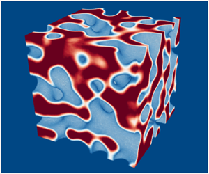
To further demonstrate the capability of the devised DFP-SP model to address realistic and challenging multi-phase flows, here we extend the study of the spinodal decomposition to three-dimensional physical space. The simulation domain is set to  $\varOmega _x=[0,L]^3\ \mathrm {m}^3$, where
 $L=3\times 10^{-8}\ \mathrm {m}$. Here,
 $\varOmega _x$ is discretized by
 $100^3$ cells. As boundary conditions, the specular reflection for particles leaving the domain as well as the Neumann boundary condition for the SP model of long-range interactions are considered. Here,
 $N_p=4.32\times 10^8$ particles and a time step size of
 ${\rm \Delta} t= 2\times 10^{-14}$ s are considered. Initially, we sample the position of particles inside
 $\varOmega _x$ from a uniform distribution with a weight that provides us with the initial number density of
 $n^{(0)}=8\times 10^{27}\ \mathrm {m^{-3}}$. Furthermore, similar to the two-dimensional case, the velocity of particles are initialized by sampling from the Maxwellian distribution such that we obtain the initial temperature of
 $T^{(0)}=120\ \mathrm {K}$.
Having employed similar computational resources like that for the two-dimensional case, we observe that the average execution time for  $50$ iterations per cell approximately ranges from
 $600~\mathrm {s}$ to
 $2040~\mathrm {s}$. Here, the effect of load imbalance due to particle clustering is more pronounced. Hence, we acknowledge the need for devising an efficient load balancing scheme that benefits from density distribution in the physical space, in parallel computations of multi-phase flows using particles. Similar to test case (C), as shown by the evolution of number density in figure 23 and more profoundly in supplementary movie 4, we observe the formation of bubbles contained in the liquid. Simulation results of this spinodal decomposition using the DFP-SP model was carried out until
 $t_{{final}}\approx 0.304\ \mathrm {ns}$ with a time step size of
 ${\rm \Delta} t=0.02\ \mathrm {ps}$ which took about
 $3$ days.
Evolution of normalized number density for the spinodal decomposition of argon in three-dimensional physical space  $\varOmega _x=[0,L]^3\ \mathrm {m}^3$, where
 $L=3\times 10^{-8}\ \mathrm {m}$ obtained from simulation results of the DFP-SP model, with initial number density
 $n^{(0)}=8\times 10^{27}\ \mathrm {m}^{-3}$ and temperature
 $T^{(0)}= 120\ \mathrm {K}$.

Finally, we provide a rough estimate on the computational cost of the devised DFP-SP in comparison to the standard MD algorithm, for a fixed statistical noise and time step size. Given the volume of the domain and the number density, there are  $N_\text {mol}=216\times 10^{3}$ physical molecules inside the cube. In order to control the noise in observables, e.g. bulk velocity, the MD simulation should be averaged over an ensemble of
 $N_{{ens}}$ snapshots. By repeating the MD simulation
 $N_\text {ens}$ times, one can obtain the variance of
 $\epsilon ^2\propto 1/(N_\text {mol}N_\text {ens})$. In the case of our particle solver, we deployed
 $N_p=4.32\times 10^{8}$ samples which lead to the noise of
 $\epsilon ^2\propto 1/N_p=2.3\times 10^{-9}$. To obtain similar noise with MD, one would need to use
 $N_\text {ens}\approx 2000$ samples. Hence the total number of operations for one time step of MD becomes
 $N_\text {ens}N_\text {mol}^2\approx 9\times 10^{13}$.
However, the number of operations for DFP-SP is linear with  $N_p =4.32\times 10^{8}$ resulting in a significant speed-up compared with MD. Note that while introducing a cut-off leads to faster MD simulations, still the cost remains significantly higher than DFP-SP as the latter does not explicitly compute short-range interactions.
8. Conclusion and outlook
Multi-phase flows far from the equilibrium demand for high-fidelity models beyond the conventional hydrodynamics. This study lays out a Fokker-Planck-Poisson approach which systematically reduces the multi-phase kinetic description into a set of SDEs suitable for efficient particle simulations. The short-range molecular collisions are described by the dense FP model, whereas the long-range interactions are cast into a SP elliptic model. The resulting system then is simulated using a particle Monte-Carlo scheme in combination with a fast elliptic solver. First the accuracy and performance of the devised DFP-SP model are assessed in predicting the surface tension and the evaporation rate of a liquid slab once in contact with the vacuum and once in contact with the equilibrium vapour phase. Furthermore, two intriguing multi-phase problems were addressed. The inverted temperature gradient phenomenon, which is observed in the vapour phase contained between two liquid slabs kept at slightly different temperatures, was accurately reproduced by the DFP-SP model. Further insights into the phenomenon were gained by analysing a single droplet evaporation process. Next, the spinodal decomposition of argon was investigated at different initial densities. The formation and coalescence of bubbles as well as droplets are illustrated. Moreover, the droplet growth rates are found to be consistent with the Lifschitz–Slyozov solution. Future steps will focus on integration of more accurate molecular potentials such as the Lennard–Jones potential into the Fokker-Planck-Poisson framework. We expect that this can be achieved by employing a system of SP equations. Moreover, extension of the model towards polyatomic degrees of freedom, mixtures and chemical reactions will be pursued.
Supplementary movies
Supplementary movies are available at https://doi.org/10.1017/jfm.2021.461.
Acknowledgements
The authors would like to thank the anonymous reviewers for their valuable and constructive comments and suggestions which improved the quality of the paper. The authors gratefully acknowledge the supports of M. Torrilhon throughout this study. Furthermore, we appreciate the stimulating discussions with P. Jenny.
Funding
This work was supported by the Deutscher Akademischer Austauschdienst (M.S., grant numbers 57438025); the Swiss National Science Foundation (H.G., grant number 174060); and the Deutsche Forschungsgemeinschaft (M.P., grant number 393159129).
Declaration of interests
The authors report no conflict of interest.
Appendix A. ESMC-Vlasov solution algorithm
Here first the Monte-Carlo approach to account for the Enskog equation, i.e. ESMC, is reviewed. Then, the direct approach in solving the Vlasov integral is explained. At the end, the combined ESMC-Vlasov algorithm is presented which is deployed in this work as the benchmark solution of the EV equation. For more details on the DSMC approach for flow simulation based on the EV equation, see Frezzotti et al. (Reference Frezzotti, Barbante and Gibelli2019).
Consider the position  $X$ and the velocity
 $V$ as random variables which describe the evolution of
 $\mathcal {F}$ in the EV equation. As a Monte-Carlo particle method, instead of solving for
 $\mathcal {F}$ directly, the samples of position and velocity are evolved. Hence, at each time step, first the velocity of particles are evolved following a jump process. Then, particles with new velocities are streamed freely till the end of the time step.
A.1. ESMC collision step
The modified ESMC solution algorithm was introduced to mimic the solution algorithm of classical Bird's DSMC method with the modification for collision frequency as well as incorporating the fact that the colliding pair might lie in different cells. Using Bird's no-time-counter approach (Bird Reference Bird1994), particles collide with the probability of
 \begin{equation} \mathcal{P}_{{coll.}} = \frac{\sigma_T c_r Y(n_{{mid}})}{\{\sigma_T c_r Y(n_{{mid}})\}_{max}}, \end{equation}
where  $\sigma _T={\rm \pi} \sigma ^2$ is the hard-sphere collision cross-section,
 $g_r$ the magnitude of relative velocity for a colliding pair with number density of
 $n_{{mid}}$ at their midpoint. Here, the subscript max indicates an upper limit for the values of
 $\sigma _T c_r$ in the computational cell. A particle pair with the index
 $(i,j)$ collides while satisfying the conservation laws. Bringing the randomness in the post-collision direction of velocity, the velocity of the colliding pair during a collision evolves as
 $$\begin{gather} {V}^{(i)} = V_{{c}} + \frac{{g}}{2} \quad \text{and} \end{gather}$$
 $$\begin{gather}{V}^{(\,j)} = V_{{c}} - \frac{{g}}{2}, \quad \text{where} \end{gather}$$
 $$\begin{gather}{g} = g_r [\cos(\theta), \sin(\theta)\cos(\phi), \sin(\theta)\sin(\phi)]^\textrm{T}. \end{gather}$$
Consistent with the hard-sphere model, the angles of the post-collision relative velocity  $g$ are drawn randomly with the uniform probability on the surface of the ball
 $\mathcal {B}(0,1)$ which is centred at zero and has the unit radius. Due to efficiency in sampling from one-dimensional uniform distribution in practice, the angles
 $\theta$ and
 $\phi$ can be easily sampled using the map
 $$\begin{gather} \theta = \mathrm{arccos}( 2 \alpha_1-1 ) \quad \text{and} \end{gather}$$
 $$\begin{gather}\phi = 2 {\rm \pi}\alpha_2, \end{gather}$$
where  $\alpha _{1,2} \sim \mathcal {UR}([0,1])$, i.e. continuous uniform distribution with support in the interval
 $[0,1]$. The velocity of centre of mass
 $V_{{c}}:= ( V^{(i)}+ V^{(\,j)})/2$ and the magnitude of relative velocity
 $g:= V^{(i)}- V^{(\,j)}$, i.e.
 $g_r:=|g|$, remain constant during elastic collisions. Let
 $\hat {k}$ indicate the unit vector with the direction pointing to the centre of the
 $j$th particle from the
 $i$th particle's centre of mass. Hence, the number of collision candidates
 $N_{{cand}}^{(I)}$ for the time step size
 ${\rm \Delta} t$ in the cell with index
 $I$ and
 $N_p^{(I)}$ particles is
 $$\begin{gather} N_{{cand}}^{(I)} = \tfrac{1}{2} \omega_{{max}}^{(I)} N_p^{(I)},\quad \textrm{where} \end{gather}$$
 $$\begin{gather}w^{(I)}_{{max}} = 4 {\rm \pi}\sigma^2 max_{(ij)}\{(g,k) n^{(J)} Y (n_{{mid}}) \} {\rm \Delta} t. \end{gather}$$
We initialize the upper bound of the collision rate using the thermal velocity
 \begin{equation} \omega_{{max},0}^{(I)} = 4 {\rm \pi}\sigma^2 n^{(I)} \varTheta_0^{(I)} Y(n^{(I)}) {\rm \Delta} t ,\quad \textrm{where}\ \varTheta_0^{(I)} = 10 \sqrt{\frac{k T_0^{(I)}}{m}}, \end{equation}
and update it every time step if a collision with  $\omega ^{(ij)}>w^{(I)}_{{max}}$, where
 \begin{equation} \omega^{(ij)}:=4 {\rm \pi}\sigma^2 (g,\hat{k}) n^{(J)} Y (n_{{mid}}) {\rm \Delta} t \end{equation}
occurs. Details of the implemented solution algorithm is described in algorithm 2. Note that here,  $\mathcal {UI}([a,b])$ for
 $a,b \in \mathbb {N}$ and
 $b\geq a$ indicates a uniform discrete distribution over the set of natural numbers between
 $a$ and
 $b$. Furthermore, simply looping over cells and performing Enskog collisions similar to the implementation of DSMC may lead to introducing bias due to outside cell collisions and the fact that particles of one cell always are considered for collision before another. Therefore, an unbiased particle selection algorithm is devised here for the ESMC algorithm.
Collision step of ESMC

A.2. Numerics of long-range interaction
Similar to the SP model, first the Vlasov integral is estimated numerically on the faces of the computational cell indexed  $(i,j,k)$. It is simpler to take the integral in spherical coordinates and read the density of the quadrature points from the density field. Then, the numerical estimate of the Vlasov integral with its origin at the centre of the face that is indexed by
 $f_l$ becomes
 $$\begin{gather} U_{f^{(i,j,k)}_l}^{(n)} = \phi_0 \sum_{\alpha=1}^{N_r} \sum_{\beta=1}^{N_{\phi}} \sum_{\gamma=1}^{N_{\theta}} \left(\frac{\sigma}{r^{(\alpha)}}\right)^6 n (y^{(\alpha,\beta,\gamma)}) (r^{(\alpha)})^2 \sin(\phi^{(\beta)}) {\rm \Delta} r^{(\alpha)} {\rm \Delta} \phi^{(\beta)} {\rm \Delta} \theta^{(\gamma)}, \end{gather}$$
 $$\begin{gather}y^{(\alpha,\beta,\gamma)} = ( r^{(\alpha)} \cos(\theta^{(\gamma)}) \sin(\phi^{(\beta)}), r^{(\alpha)} \sin(\theta^{(\gamma)}) \sin(\phi^{(\beta)}), r^{(\alpha)} \cos(\phi^{(\beta)}) )^\textrm{T}. \end{gather}$$
Let us combine the variables in a vector  $x=[r, \phi , \theta ]^\textrm {T}$ with lower and upper bounds in vectors
 $a=[\sigma , 0, 0]^\textrm {T}$ and
 $b=[r_{{cut}}, {\rm \pi}, 2{\rm \pi} ]^\textrm {T}$, respectively. For numerical integration, Legendre–Gauss quadrature rule using
 $N_r=N_\phi =N_\theta =10$ are employed here. The
 $\eta$th quadrature weight
 $w$ and point
 $\xi$ from the standard interval
 $[-1,1]$ are simply mapped back to the interval of interest for the
 $s$th component of
 $x$ via
 $$\begin{gather} x_{s}^{(\eta)} = \xi^{(\eta)} \frac{b_s-a_s}{2} +\frac{a_s+b_s}{2}\quad \textrm{and} \end{gather}$$
 $$\begin{gather}{\rm \Delta} x_{s}^{(\eta)} = w^{(\eta)} \frac{b_s-a_s}{2}. \end{gather}$$
Once the potential on the faces are computed numerically, the attractive forces are estimated via finite differences.
A.3. ESMC-Vlasov algorithm
To combine long-range interaction along with the short-range one, first at each time step, the ESMC collision step is carried out. Then, the velocities are updated to include attractive contribution once the numerical integration of the Vlasov on the faces are evaluated. Algorithm 3 shows the outline of the ESMC-Vlasov solution algorithm used as the benchmark in this study.
ESMC-Vlasov algorithm

Appendix B. Hybridized discontinuous Galerkin solver
The solver used for the screened Poisson equation in the parallel high performance computing case is based on the hybridized discontinuous Galerkin solver in the particle code PICLas (Fasoulas et al. Reference Fasoulas, Munz, Pfeiffer, Beyer, Binder, Copplestone, Mirza, Nizenkov, Ortwein and Reschke2019). This solver uses a spectral element representation and is therefore referred to as the hybridized discontinuous Galerkin spectral element method (HDGSEM). The main advantage of this method is its reasonably high performance in parallelization. Here, an overview and introduction of the concept is given. The detailed derivation of the method as well as its application in simulations of plasma physics can be found in Pfeiffer et al. (Reference Pfeiffer, Hindenlang, Binder, Copplestone, Munz and Fasoulas2019).
As a first step, the screened Poisson equation (4.8) is decomposed into a first-order system of PDEs, i.e.
 \begin{equation} \lambda^2 u - \frac{\partial q_i}{\partial x_i} = n,\quad q_i = \frac{\partial u}{\partial x_i}, \end{equation}
with Dirichlet and Neumann boundary conditions encoded by
 \begin{equation} u |_{\partial \varOmega_{Dir}}=u_{Dir},\quad q_i \tilde{n}_i |_{\partial \varOmega_{Neu}}={( q_i \tilde{n}_i)}_{Neu}. \end{equation}
Here,  $\tilde {n}$ denotes the outward unit normal vector on the boundary surface of the domain. One can obtain the variational form by multiplying the equations with test functions
 $\bar {u}$ and
 $\bar {q}$, respectively, and integrate over the volume of each element
 $K$, i.e.
 $$\begin{gather} \langle \lambda^2 u,\bar{u} \rangle_K - \left\langle \frac{\partial q_i}{\partial x_i},\bar{u} \right\rangle_K = \langle n,\bar{u} \rangle_K, \end{gather}$$
 $$\begin{gather}\langle q_i,\bar{q}_i \rangle_K = \left\langle \frac{\partial u}{\partial x_i} ,\bar{q}_i \right\rangle_K. \end{gather}$$
Here,  $\langle a_i, b_i\rangle _K$ denotes the integration of the inner product
 $a_ib_i$ inside the Kth element. Next, these equations are integrated by parts and discontinuous solutions at element interfaces are allowed for
 $q$ by applying jump condition. The main idea of HDGSEM is to introduce an additional unknown
 $\theta$, which is unique on each element interface, in order to reduce dimension of the global system to the number of interfaces. By skipping several steps in the derivation, the final system of equations including the auxiliary variable
 $\theta$ as well as stabilization parameter
 $\tau >0$, see Cockburn et al. (Reference Cockburn, Dong, Guzmán, Restelli and Sacco2009), can be obtained as
 $$\begin{gather} \langle \lambda^2 u,\bar{u}\rangle_K + \left\langle \frac{\partial q_i}{\partial x_i}, \bar{u}\right\rangle _K -\sum_{e\in\partial K}\{\tau u \bar{u}\}_e +\sum_{e\in\partial K}\{\tau \theta \bar{u}\}_e = \langle n,\bar{u}\rangle _K, \end{gather}$$
 $$\begin{gather}\langle q_i,\bar{q}_i\rangle _K + \left\langle u, \frac{\partial \bar{q}_i}{\partial x_i}\right\rangle _K -\sum_{e\in\partial K}\{\theta \bar{q}_i \tilde{n}_i\}_e =0, \end{gather}$$
 $$\begin{gather}\textrm{and}\quad \sum_{e\in\partial K, K'}(\{ q_i \tilde{n}_i \bar{\theta}\}_e + \{\tau u \bar{\theta}\}_e - \{\tau \theta \bar{\theta}\}_e ) = \sum_{e\in\varOmega_{Neu}} \{ q_i \tilde{n}_i \bar{\theta}\}_e, \end{gather}$$
with the adjacent element  $K'$ on the interface indicated by
 $e$. Note that here
 $\{s\}_e$ indicates average of
 $s$ on the edge
 $e$; see Arnold et al. (Reference Arnold, Brezzi, Cockburn and Marini2002). For the sake of simplicity, the transformation to/from the reference space is not explained here. This transformation as well as a detailed derivation of (B5)–(B7) can be found in Pfeiffer et al. (Reference Pfeiffer, Hindenlang, Binder, Copplestone, Munz and Fasoulas2019).
In order to find the solution  $u$ of (B1), first, a global system of equations is solved for the auxiliary variable
 $\theta$ only on the surfaces using a conjugate-gradient method. The final volume solution
 $u$ inside each cell is calculated in a post-processing step locally in each element. Once the solution
 $u$ with expansion in polynomial basis functions inside each cell is found, its derivatives needed for computing attractive force
 $H$ at any point inside the cell can be obtained simply by applying derivatives on the basis functions.
Appendix C. Total energy for EV system
In order to derive evolution of the total energy in the EV equation, let us first multiply (2.3) by  $v_jv_j/2$ and integrate over
 $v$. Therefore, we get
 \begin{equation} \frac{\partial}{\partial t}\int_{\mathbb{R}^3} \frac{1}{2}\mathcal{F} v_jv_j\, \textrm{d} v+\frac{\partial }{\partial x_i}\left(\frac{1}{2}\int_{\mathbb{R}^3} v_i v_jv_j\mathcal{F} \, \textrm{d} v\right)-\int_{\mathbb{R}^3} v_j\frac{H_j}{m}\mathcal{F}\, \textrm{d} v= 0. \end{equation}
Using the notation
 \begin{equation} \mathbb{E}[Q(V|x,t)]=\frac{1}{\rho}\int_{\mathbb{R}^3} Q(v)\mathcal{F}(v,x,t)\, \textrm{d} v, \end{equation}
yields
 \begin{equation} \frac{\partial}{\partial t}\left(\frac{1}{2}\rho \mathbb{E}[V_jV_j|x,t]\right)+\frac{\partial}{\partial x_i}\left(\frac{1}{2}\rho \mathbb{E}[V_iV_jV_j|x,t]\right)-\frac{H_j}{m}\rho \mathbb{E}[V_j|x,t]=0. \end{equation}
Now by taking an integral over the physical space  $\varOmega$, we get
 \begin{align} &\frac{\partial}{\partial t}\int_\varOmega \left(\frac{1}{2}\rho \mathbb{E}[V_jV_j|x,t]\,{\textrm{d} x}\right)+\int_{\partial \varOmega}\left(\frac{1}{2}\rho \mathbb{E}[V_iV_jV_j|x,t]n_i\, \textrm{d} s\right)\nonumber\\ &\quad +\int_{\partial \varOmega}\left(\frac{\varPhi}{m}\rho \mathbb{E}[V_j|x,t]n_j\, \textrm{d} s\right)+\int_\varOmega \frac{\varPhi}{m}\frac{\partial \rho}{\partial t}\, {\textrm{d} x} = 0, \end{align}
where  $\partial \varOmega$ is the boundary of
 $\varOmega$ and
 $n$ its normal. Therefore, for the interval
 $t=0$ to
 $t=t_f$, we get
 \begin{align} E_{kin}(t_f)&= E_{kin}(0)-\int_0^{t_f}\int_\varOmega \frac{\varPhi}{m}\frac{\partial \rho}{\partial t}\, \textrm{d} x\, \textrm{d} t \nonumber\\ &\quad -\int_0^{t_f} \int_{\partial \varOmega} \left(\frac{1}{2}\mathbb{E}[V_iV_jV_j|x,t]+\frac{\varPhi}{m}\mathbb{E}[V_i|x,t]\right)\rho n_i\, \textrm{d} s\, \textrm{d} t, \end{align}
where  $E_{kin}=\int _\varOmega 1/2\rho \mathbb {E}[V_jV_j|x,t]\, {\textrm {d} x}$. The surface term can be computed by averaging over particles crossing the boundary of the domain. If we have the homogeneous boundary condition however, it simplifies to
 \begin{equation} E_{kin}(t_f)=E_{kin}(0)-\int_0^{t_f}\int_\varOmega \frac{\varPhi}{m}\frac{\partial \rho}{\partial t}\, \textrm{d} x\, \textrm{d} t. \end{equation}
Since  $\varPhi$ depends on
 $\rho$ through a time-independent symmetric kernel
 \begin{equation} \varPhi( x,t)= \int_\varOmega \mathcal{K}( x^\prime, x) \rho( x^\prime,t)\, {\textrm{d} x}^\prime, \end{equation}
we obtain
 \begin{equation} \frac{\partial \varPhi}{\partial t}= \int_\varOmega \mathcal{K} \frac{\partial \rho}{\partial t}\, {\textrm{d} x}, \end{equation}
and, thus,
 \begin{align} \int_\varOmega \rho \frac{\partial \varPhi}{\partial t}\, {\textrm{d} x}&= \int_\varOmega \rho( x) \int_\varOmega \mathcal{K}( x^\prime , x) \frac{\partial \rho ( x^\prime)}{\partial t}\, {\textrm{d} x}^\prime \, {\textrm{d} x} \nonumber\\ &= \int_\varOmega \frac{\partial \rho( x^\prime)}{\partial t} \int_\varOmega \mathcal{K}( x^\prime , x) \rho( x)\, {\textrm{d} x}\, {\textrm{d} x}^\prime \end{align}
 \begin{align} &= \int_\varOmega \frac{\partial \rho( x^\prime)}{\partial t} \int_\varOmega \mathcal{K}( x , x^\prime) \rho( x) \, \textrm{d} x\, \textrm{d} x^\prime \end{align}
 \begin{align} &= \int_\varOmega \frac{\partial \rho }{\partial t}\varPhi \, {\textrm{d} x}^\prime. \end{align}
Therefore, (C6) results in the energy conservation
 \begin{equation} E_{kin}(t_f)+E_{pot}(t_f)=E_{kin}(0)+E_{pot}(0), \end{equation}
where  $E_{pot}=1/2\int _\varOmega \rho \varPhi /m\, {\textrm {d} x}$ is the potential energy.