



1. Introduction
Water is at the origin of life and a fundamental element for human survival and development. Only after learning to navigate the waves of the ocean were humans able to exploit its potential and explore the world. Close to the water surface, buzzing with a multitude of biological processes (Sieburth et al. Reference Sieburth, Willis, Johnson, Burney, Lavoie, Hinga, Caron, French, Johnson and Davis1976; Carlson & Mayer Reference Carlson and Mayer1980), the complex interplay between surface winds and oceanic currents takes place on a variety of scales. Locally, fluid mixing (Zappa et al. Reference Zappa, McGillis, Raymond, Edson, Hintsa, Zemmelink, Dacey and Ho2007) and wave breaking (Peregrine Reference Peregrine1983; Perlin et al. Reference Perlin, Choi and Tian2013; Romero Reference Romero2019; Deike Reference Deike2022) enhance gas exchange with the atmosphere (Liss & Slater Reference Liss and Slater1974) (e.g. carbon dioxide absorption in the water). On geophysical scales, evaporation and momentum exchange between the atmosphere and the ocean drive intense climatic events (Li et al. Reference Li, Zahariev and Garrett1995; Hu et al. Reference Hu2015; Caesar et al. Reference Caesar, Rahmstorf, Robinson, Feulner and Saba2018). Severe weather phenomena such as typhoons and hurricanes pose a significant hazard to human survival (Li & Chakraborty Reference Li and Chakraborty2020), while tsunamis are becoming increasingly dangerous with growing sea levels (Chua et al. Reference Chua, Otake, Li, Cheng, Qiu, Li, Suppasri, Imamura and Switzer2024; Shi et al. Reference Shi, Feng, Toumi, Zhang, Hodges, Tao, Zhang and Zheng2024). From an engineering perspective, winds, waves and currents offer potential avenues for energy production (Egbert & Ray Reference Egbert and Ray2000; Gonzalez et al. Reference Gonzalez2024; Lu et al. Reference Lu, Zhao, Fu, Yeatman, Ding and Chen2024; Robertson et al. Reference Robertson, Musial, Shields, Aubault, Ikari and Kitzing2025).
Air–water interactions in the upper ocean layer, and the dynamics of the interface between them, often occur at high Reynolds numbers, where inertial forces dominate over viscous effects, and the resulting fluid motion is chaotic and turbulent (Hartline Reference Hartline1979; Nimmo Smith et al. Reference Nimmo Smith, Thorpe and Graham1999; Jones & Toba Reference Jones and Toba2001; D’Asaro et al. Reference D’Asaro, Lee, Rainville, Harcourt and Thomas2011). Understanding how flow turbulence and surface waves interact is therefore of central importance. Although subsurface turbulence often triggers complex surface dynamics (Savelsberg & van de Water Reference Savelsberg and van de Water2008, Reference Savelsberg and van de Water2009), the precise nature of these motions remains unclear. In particular, it is still an open question as to when the surface deforms primarily under the direct influence of flow turbulence, described by Kolmogorov’s K41 theory (Kolmogorov Reference Kolmogorov1941), and when it develops a distinct form of turbulent motion – the so-called wave turbulence (Newell & Rumpf Reference Newell and Rumpf2011; Falcon & Mordant Reference Falcon and Mordant2022) – arising from nonlinear wave–wave interactions.
Several kinds of waves have been observed on the ocean surface and multiple theoretical approaches have been proposed to describe their chaotic dynamics (Craik Reference Craik2004; Nazarenko & Lukaschuk Reference Nazarenko and Lukaschuk2016), ranging from weakly nonlinear wave turbulence theories, where resonant wave–wave interactions drive energy cascades across scales (Zakharov & Filonenko Reference Zakharov and Filonenko1967; Newell & Rumpf Reference Newell and Rumpf2011; Nazarenko & Lukaschuk Reference Nazarenko and Lukaschuk2016; Falcon & Mordant Reference Falcon and Mordant2022), to models in which the interface is forced directly by turbulent pressure fluctuations in the flow (Bhunia & Lienhard Reference Bhunia and Lienhard1994), leading to Phillips and Toba-type equilibrium ranges in the wave spectrum (Phillips Reference Phillips1957; Toba Reference Toba1973; Phillips Reference Phillips1985; Ryabkova et al. Reference Ryabkova, Karaev, Guo and Titchenko2019). A linear-response framework was developed by Perrard et al. (Reference Perrard, Lozano-Durán, Rabaud, Benzaquen and Moisy2019) to describe the deformation of a liquid surface subject to turbulent forcing in wind-driven conditions.
Brocchini & Peregrine (Reference Brocchini and Peregrine2001) classified the possible surface responses in terms of Froude and Weber numbers based on the integral scale and root-mean-square velocity of the underlying flow turbulence, emphasising the competition between turbulent forcing and gravitational and capillary restoring effects. More recently, dedicated experimental and numerical studies have sought to relate observable surface features to the underlying turbulent flow (Ruth & Coletti Reference Ruth and Coletti2026; Babiker et al. Reference Babiker, Aarnes, Semati, Ferran, Tee, Hearst and Ellingsen2026; Ferran et al. Reference Ferran, Semati, Rouaud, Hearst and Ellingsen2026). These studies demonstrate that surface deformation contains quantitative information about subsurface turbulence, while also highlighting the importance of the near-surface flow and, in the presence of a mean current, of Doppler shifting in the observed wave dispersion relation (Ferran et al. Reference Ferran, Semati, Rouaud, Hearst and Ellingsen2026).
When their amplitude is large enough, waves propagating at the water surface might also induce turbulent motions in the neighbouring fluid, the so-called wave-induced-turbulence (Babanin Reference Babanin2006). However, the relative importance of the mechanisms listed above remains unsettled. Experiments and simulations are being developed to clarify this, yet each approach has limitations. Laboratory experiments (Michel et al. Reference Michel, Pétrélis and Fauve2017; He et al. Reference He, Slunyaev, Mori and Chabchoub2022; Feddersen et al. Reference Feddersen, Fincham, Brodie, Young, Spydell, Grimes, Pieszka and Hanson2023; Smeltzer et al. Reference Smeltzer, Rømcke, Hearst and Ellingsen2023) have traditionally been restricted by the finite size of the facility and the resulting limited inertial range, although recent investigations have substantially broadened the range of turbulent conditions accessible at the free surface (Babiker et al. Reference Babiker, Aarnes, Semati, Ferran, Tee, Hearst and Ellingsen2026; Berhanu & Falcon Reference Berhanu and Falcon2026; Ruth & Coletti Reference Ruth and Coletti2026). Numerical simulations likewise face finite-size effects associated with periodic domains, which limit the range of accessible wavelengths and therefore the scale separation over which asymptotic behaviour can be identified. In addition, many numerical studies (Onorato et al. Reference Onorato, Osborne and Serio2006; Baronio et al. Reference Baronio, Conforti, Degasperis, Lombardo, Onorato and Wabnitz2014; Dyachenko et al. Reference Dyachenko, Kachulin and Zakharov2017) often solve Schrödinger-like equations (Lo & Mei Reference Lo and Mei1985; Dysthe Reference Dysthe1997) that neglect viscous effects and strong nonlinearities, potentially hindering – or even preventing – the emergence of turbulent dynamics. Only in recent years have fully resolved, nonlinear multiphase simulations been performed to study wave breaking (De Vita et al. Reference De Vita, Verzicco and Iafrati2018; Chan et al. Reference Chan, Johnson, Moin and Urzay2021; di Giorgio et al. Reference di Giorgio, Pirozzoli and Iafrati2022; Wu et al. Reference Wu, Popinet and Deike2022) and propagation (Zonta et al. Reference Zonta, Soldati and Onorato2015; Giamagas et al. Reference Giamagas, Zonta, Roccon and Soldati2023; Matsuda et al. Reference Matsuda, Komori, Takagaki and Onishi2023), with the latter often yielding results in apparent contradiction with earlier experimental observations due to the inherent difficulty of matching the regimes where simulations and experiments are performed.
Despite this progress, most existing approaches focus either on intrinsic surface dynamics, as in wave turbulence theories, or on their direct forcing by turbulence, and a general framework that consistently couples bulk turbulent motions to the dynamics of a deformable interface (i.e. turbulence-induced waves) is still missing.
Here we take a fundamental step forward in understanding the interplay between flow turbulence and surface dynamics by establishing the theoretical foundations of the interaction. Our theory applies when the direct response to turbulent pressure fluctuations, together with the linear restoring and damping mechanisms, controls the surface statistics on the time scales considered, while nonlinear spectral redistribution remains subleading. It ceases to apply when the nonlinear transfer becomes dynamically comparable to these processes. Under these constraints, we isolate two distinct dynamical regimes for surface motion. In the first, intrinsic surface dynamics is faster than the surrounding flow turbulence, and emerges. In the second it is slower, so the surface is enslaved by the turbulent forcing and exhibits either an inertia-dominated or a viscous-dominated response depending on the system parameters. We validate our theoretical predictions by performing state-of-the-art, fully resolved nonlinear simulations. The quasi-realistic, turbulence-driven wave system shown in figure 1 conforms to our theoretical predictions in the regime where surface dynamics outpaces the turbulent forcing. When surface dynamics is slower, by contrast, fluid–fluid interfaces tend to break; we therefore support the theory with measurements performed on the surface of a hyperelastic solid exposed to a turbulent flow, used specifically to test the slow, viscous-dominated enslaved limit in which the precise form of the restoring mechanism does not enter at leading order. We therefore not only validate our theoretical framework introducing state-of-the-art simulations, but also show that its scope extends beyond the water-surface dynamics for which it was conceived: this work provides a powerful, unifying framework for the dynamics of free surfaces in turbulence.
Interplay between flow turbulence and surface waves. We visualise the multiphase air–water flow over a smooth bed, as captured by our fully resolved nonlinear simulations. Turbulence develops in the water due to friction at the bed and spreads towards the surface, agitated by pressure fluctuations. Surface waves develop and propagate, perturbing the overlying wind through the formation of hairpin-like vortical structures. The dynamics of air and water is thus fully turbulent, as well as that of the surface separating them, which is the subject of our investigation.

Figure 1. Long description
A diagram of the interaction between air and water flow. The diagram shows a three-dimensional representation of the multiphase air-water flow over a smooth bed. The flow is visualized with different colors indicating vorticity magnitude, negative pressure, and positive pressure. The surface waves and turbulent structures are depicted, with arrows indicating the direction of flow and pressure fluctuations. The diagram includes labels for vorticity magnitude, negative pressure, and positive pressure, and shows the interaction between the air and water phases.
2. Theoretical framework
Consider the interface separating two immiscible and incompressible fluids of density
 $\rho _1,\rho _2$
and kinematic viscosity
 $\nu _1,\nu _2$
, respectively. Subscript 1 denotes the lighter fluid phase over the interface and subscript 2 the heavier one below. Decomposing the interfacial displacement
 $\eta$
in its Fourier modes
 $\hat \eta _{\boldsymbol{\kappa }}$
at each wavenumber
 $\boldsymbol{\kappa }$
,
 \begin{align} {\eta (x,z,t)=\iint \hat \eta _{\boldsymbol{\kappa }}(t) {\rm e}^{\mathrm i(\kappa _xx+\kappa _zz)}\,\mathrm d^2\kappa ,\quad \text{with } \boldsymbol{\kappa }=(\kappa _x,\kappa _z),\quad \kappa =|\boldsymbol{\kappa }|,} \end{align}
the linearised equation (Phillips Reference Phillips1957; Li & Shen Reference Li and Shen2023) for each mode is written as a canonical forced and damped oscillator (details of the derivation can be found in Appendix A):
 \begin{align} \ddot {\hat \eta }_{\boldsymbol{\kappa }} +2\frac {(\rho _1\nu _1+\rho _2\nu _2)\kappa ^2}{\rho _1+\rho _2}\,\dot {\hat \eta }_{\boldsymbol{\kappa }} +\frac {\bigl [(\rho _2-\rho _1)g\kappa +\sigma \kappa ^{3}\bigr ]}{\rho _1+\rho _2}\hat \eta _{\boldsymbol{\kappa }} =-\frac {\kappa }{\rho _1+\rho _2}\,\widehat {\Delta p'}_{\boldsymbol{\kappa }}(t). \end{align}
Here, dotted quantities have been differentiated in time,
 $g$
represents the magnitude of the gravity vector,
 $\sigma$
is the surface tension and
 $\widehat {\Delta p'}$
is the fluctuating part of the pressure jump across the interface. We identify the coefficients of (2.2) with twice the damping and the squared natural frequency of the system, respectively:
 \begin{align} \fbox{$\gamma (\kappa )={(\rho _1\nu _1+\rho _2\nu _2)\kappa ^{2}}/({\rho _1+\rho _2})$} \quad \text{and} \quad \fbox{$\omega _0^{2}(\kappa )={ \big[(\rho _2-\rho _1)g\,\kappa +\sigma \kappa ^{3} \big]}/({\rho _1+\rho _2}).$} \end{align}
Equation (2.2) can therefore be interpreted as a forced resonant oscillator: for each wavenumber
 $\kappa$
, the natural frequency
 $\omega _0(\kappa )$
is set by the gravity–capillary dispersion relation, while
 $\gamma (\kappa )$
controls the dissipative broadening of the resonance. The turbulent pressure fluctuations then provide the broadband forcing that excites this response. Fluctuating tangential stresses at the interface would provide an additional forcing term in the linear response, as considered by Perrard et al. (Reference Perrard, Lozano-Durán, Rabaud, Benzaquen and Moisy2019). Such a contribution is relevant for shear-dominated configurations, e.g. wind-driven waves, whereas the present work focuses on interfaces driven by pressure fluctuations generated by turbulence in the flow. This framework should therefore not be extrapolated to describe shear-driven surface dynamics in its present form, while extensions in the spirit of Perrard et al. (Reference Perrard, Lozano-Durán, Rabaud, Benzaquen and Moisy2019) are possible yet out of scope. Additionally, the derivation above is a linearised description and does not contain nonlinear wave–wave interactions, formally assuming
 $\kappa \eta \lt 1$
at each scale of interest. It is therefore not intended to describe strongly nonlinear or breaking waves, nor wave turbulence regimes in which resonant interactions provide the leading transfer of energy across scales.
Applying Fourier’s transform in time to (2.2) according to the the convention
 \begin{align} \widehat {\eta }_{\boldsymbol{\kappa }}(\omega ) = \int _{-\infty }^{\infty } \widehat {\eta }_{\boldsymbol{\kappa }}(t) {\rm e}^{{\rm i}\omega t}\,\mathrm{d}t, \end{align}
with inverse transform
 \begin{align} \widehat {\eta }_{\boldsymbol{\kappa }}(t) = \frac {1}{2\pi } \int _{-\infty }^{\infty } \widehat {\eta }_{\boldsymbol{\kappa }}(\omega ) {\rm e}^{-{\rm i}\omega t}\,\mathrm{d}\omega , \end{align}
we find
 \begin{align} \hat \eta _{\boldsymbol{\kappa }}(\omega )= \frac {-\kappa \,\widehat {\Delta p'}_{\boldsymbol{\kappa }}(\omega )} {(\rho _1+\rho _2)\!\bigl [- \big(\omega ^{2}-\omega _0^{2} \big)-2\mathrm i\gamma \omega \bigr ]} \end{align}
in the domain of the frequencies
 $\omega$
, and isolate the transfer function
 \begin{align} |H(\kappa ,\omega )|^{2}\equiv \frac {1}{(\rho _1+\rho _2)^{2}} \frac {\kappa ^2\,}{\bigl (\omega ^{2}-\omega _0^{2}\bigr )^{2}+4\gamma ^{2}\omega ^{2}}. \end{align}
The azimuthally integrated (isotropic) power spectral density of the surface displacement,
 $S_\eta$
, therefore relates to that of the pressure jump,
 $S_{\Delta p}$
, through
 \begin{align} S_\eta (\kappa ,\omega )=|H(\kappa ,\omega )|^{2}\,S_{\Delta p}(\kappa ,\omega ). \end{align}
Here and below, the notation
 $S(\kappa ,\omega )$
denotes a spatiotemporal spectrum, while
 $S(\kappa )\equiv \int _{-\infty }^{\infty } S(\kappa ,\omega )\,\mathrm{d}\omega$
denotes the corresponding spectrum integrated over frequency. Similarly, the surface vertical velocity,
 $S_{\dot \eta }$
, follows as
 \begin{align} {S_{\dot \eta }(\kappa ,\omega ) =\omega ^2\,\lvert H(\kappa ,\omega )\rvert ^2\,S_{\Delta p}(\kappa ,\omega ).} \end{align}
2.1. Kolmogorov’s spectrum
Kolmogorov’s theory (Kolmogorov Reference Kolmogorov1941; Monin & Yaglom Reference Monin and Yaglom1971) allows one to predict a one-dimensional pressure spectrum of the form
 \begin{align} {S_{\Delta p}(\kappa ) = C_p\,\rho ^2\,\epsilon ^{4/3}\;\kappa ^{-7/3},} \end{align}
where
 $\rho$
and
 $\epsilon$
denote the effective density and turbulent dissipation rate of the flow at the surface, respectively:
 \begin{align} \rho ^2 \equiv \rho _1^2 + \rho _2^2 \quad\text{and}\quad \epsilon ^{4/3} \equiv \big({\rho _1^2\,\epsilon _1^{4/3} + \rho _2^2\,\epsilon _2^{4/3}} \big)/ \big({\rho _1^2 + \rho _2^2} \big). \end{align}
Introducing the eddy turnover time (and its inverse) as
 \begin{align} \tau _r(\kappa )=\epsilon ^{-1/3}\kappa ^{-2/3}, \quad \fbox{$\omega _t(\kappa )=1/{\tau _r(\kappa )}=\epsilon ^{1/3}\kappa ^{2/3},$} \end{align}
the full spatiotemporal spectrum is then written as
 \begin{align} {S_{\Delta p}(\kappa ,\omega ) = S_{\Delta p}(\kappa )\;\frac {1}{\omega _t(\kappa )}\; F \Bigl (\frac {\omega }{\omega _t(\kappa )}\Bigr ), \qquad \int _{-\infty }^{\infty }F(\xi )\,\mathrm{d}\xi = 1.} \end{align}
Equation (2.13) is a similarity closure for the frequency distribution of the pressure forcing at fixed wavenumber, rather than a one-to-one correspondence
 $\omega =\omega _t(\kappa )$
. At fixed
 $\kappa$
,
 $F$
is the normalised distribution of pressure-fluctuation variance over frequency and it is assumed to have its dominant weight for
 $|\omega |=O(\omega _t)$
. Taylor advection and random sweeping instead concern the Eulerian frequency broadening observed at a fixed point. They are not used here to convert a spatial spectrum into a temporal one: the full
 $\omega$
dependence is retained and the response spectra are subsequently integrated over frequency. Mean Doppler shifting associated with interface advection is accounted for in the space–time analysis of figure 2(c). For the asymptotic estimates below we assume that
 $F$
decays ‘sufficiently’ fast and has negligible weight in the
 $|\omega -\omega _0|\lesssim \gamma$
band, and that its low-frequency core is sufficiently regularised, for instance
 $F(\xi )=O(|\xi |^{\alpha })$
as
 $\xi \to 0$
with
 $\alpha \gt 3$
. Under these assumptions, both
 $\int F(\xi )\,\xi ^{-4}\,\mathrm{d}\xi$
and
 $\int F(\xi )\,\xi ^{-2}\,\mathrm{d}\xi$
are finite constants; only these pre-factors depend on the detailed shape of
 $F$
, whereas the
 $\kappa$
-scalings derived below do not.
2.2. Regimes of motion of the surface: pressure balance
A physically transparent classification of the regimes of motion of the surface follows directly from (2.2). Multiplying it by
 $(\rho _1+\rho _2)/\kappa$
, each Fourier mode can be written as a balance between three effective pressure contributions and the turbulent forcing:
 \begin{align} \underbrace {\frac {\rho _1+\rho _2}{\kappa }\,\ddot {\hat \eta }_{\boldsymbol{\kappa }}}_{\text{inertial pressure}} +\underbrace {2(\rho _1\nu _1+\rho _2\nu _2)\kappa \,\dot {\hat \eta }_{\boldsymbol{\kappa }}}_{\text{viscous pressure}} +\underbrace {\bigl [(\rho _2-\rho _1)g+\sigma \kappa ^{2}\bigr ]\hat \eta _{\boldsymbol{\kappa }}}_{\text{restoring pressure}} =-\widehat {\Delta p'}_{\boldsymbol{\kappa }}(t). \end{align}
Consistently with the closure (2.13), the estimates below concern the turbulence-forced stationary component whose frequency integrals are controlled by the band
 $|\omega |=O(\omega _t)$
. Accordingly, at the level of scaling,
 \begin{align} \dot {\hat \eta }_{\boldsymbol{\kappa }} \sim \omega _t(\kappa )\,\hat \eta _{\boldsymbol{\kappa }}, \qquad \ddot {\hat \eta }_{\boldsymbol{\kappa }} \sim \omega _t^2(\kappa )\,\hat \eta _{\boldsymbol{\kappa }}. \end{align}
These do not identify
 $\omega _t$
with the natural surface frequency
 $\omega _0$
: the latter remains fully retained in the transfer function (2.7), while the ratio
 $\delta =\omega _0/\omega _t$
introduced below quantifies the competition between turbulent forcing and intrinsic surface dynamics.
The three effective pressures then scale as
 \begin{align} p_I \sim \frac {\rho _1+\rho _2}{\kappa }\,\omega _t^2\,\hat \eta _{\boldsymbol{\kappa }}, \qquad p_V \sim (\rho _1\nu _1+\rho _2\nu _2)\kappa \,\omega _t\,\hat \eta _{\boldsymbol{\kappa }}, \qquad p_R \sim \bigl [(\rho _2-\rho _1)g+\sigma \kappa ^2\bigr ]\hat \eta _{\boldsymbol{\kappa }}. \end{align}
Using equations (2.3) and the definition of
 $\omega _t$
, the ratios between these contributions are immediately identified as
 \begin{align} \fbox{$\delta =\frac {\omega _0(\kappa )}{\omega _t(\kappa )}$}, \qquad \fbox{$\zeta =\frac {\gamma (\kappa )}{\omega _t(\kappa )}$}, \end{align}
so that
 $p_R/p_I \sim \delta ^2$
and
 $p_V/p_I \sim \zeta$
. The interface regimes can therefore be obtained from dominant balances in (2.14). Before presenting them, we note that both
 $\delta$
and
 $\zeta$
are inherently scale-dependent, since the intrinsic frequency
 $\omega _0$
, the damping rate
 $\gamma$
and the turbulent turnover frequency
 $\omega _t$
all depend on the wavenumber
 $\kappa$
. Thus, any distinction between wave-dominated and turbulence-dominated dynamics is to be understood locally in wavenumber space. In particular,
 $\delta \gg 1$
indicates that intrinsic surface dynamics is faster than the turbulent dynamics and can emerge as surface waves, whereas
 $\delta \ll 1$
corresponds to an interface enslaved by the turbulent flow. Similarly,
 $\zeta$
compares the viscous relaxation rate of the interface with the time scale of the turbulent forcing and distinguishes the inertia-dominated and viscosity-dominated limits of the turbulence-enslaved regime.
-
(i)
 $\delta \gg 1$
(intrinsic surface dynamics is faster than turbulence dynamics, and emerges).

In this regime the restoring pressure dominates over inertia on the turbulent time scale, and viscous dissipation remains subleading provided
 $\zeta \ll \delta ^2$
, i.e.
 $p_R \gg p_I$
and
 $p_R \gg p_V$
. The leading-order balance is therefore
 \begin{align} \bigl [(\rho _2-\rho _1)g+\sigma \kappa ^2\bigr ]\hat \eta _{\boldsymbol{\kappa }} \sim -\widehat {\Delta p'}_{\boldsymbol{\kappa }}. \end{align}
The surface elevation is thus set by the restoring mechanism active at that scale:
 \begin{align} \hat \eta _{\boldsymbol{\kappa }} \sim \frac {\widehat {\Delta p'}_{\boldsymbol{\kappa }}}{(\rho _2-\rho _1)g+\sigma \kappa ^2}, \end{align}
and the crossover between gravity and capillary waves, regardless of flow turbulence, occurs when
 $ (\rho _2-\rho _1)\,g\,\kappa = \sigma \,\kappa ^3,$
yielding the critical wavenumber
 \begin{align} \fbox{$\kappa _c = \sqrt {{(\rho _2-\rho _1)\,g}/{\sigma }}.$} \end{align}
In the gravitational limit,
 $\kappa \ll \kappa _c$
, the restoring pressure is hydrostatic and
 \begin{align} \hat \eta _{\boldsymbol{\kappa }} \sim \frac {\widehat {\Delta p'}_{\boldsymbol{\kappa }}}{(\rho _2-\rho _1)g} \quad \Rightarrow \quad \fbox{$S_{\eta }(\kappa )\propto S_{\Delta p}(\kappa )\propto \kappa ^{-7/3}.$} \end{align}
In the capillary limit,
 $\kappa \gg \kappa _c$
, curvature provides the restoring pressure and
 \begin{align} \hat \eta _{\boldsymbol{\kappa }} \sim \frac {\widehat {\Delta p'}_{\boldsymbol{\kappa }}}{\sigma \kappa ^2} \quad \Rightarrow \quad \fbox{$S_{\eta }(\kappa )\propto \kappa ^{-4}S_{\Delta p}(\kappa )\propto \kappa ^{-19/3}.$} \end{align}
Although the amplitude is selected by the intrinsic restoring dynamics, the temporal modulation remains imposed by the turbulent forcing; hence,
 \begin{align} S_{\dot \eta }(\kappa )\sim \omega _t^2(\kappa )\,S_{\eta }(\kappa ) \quad \Rightarrow \quad \fbox{$ S_{\dot \eta }(\kappa )\propto \begin{cases} \kappa ^{-1}, & \text{gravitational limit},\\[4pt] \kappa ^{-5}, & \text{capillary limit}. \end{cases}$} \end{align}
-
(ii)
$\delta \ll 1$
(surface dynamics is slower than turbulence dynamics, and the surface is enslaved by flow turbulence).

The restoring pressure is now too slow to react on the turbulent time scale, so the response is controlled by whichever term, inertia or viscous dissipation, balances the pressure forcing most efficiently.
-
(a)
$\zeta \ll 1$
(inertia-dominated enslaved limit): viscous effects are weak on the turbulent time scale, so the forcing balances the effective interfacial inertia:(2.24)Using equation (2.15),
\begin{align} \frac {\rho _1+\rho _2}{\kappa }\,\ddot {\hat \eta }_{\boldsymbol{\kappa }} \sim -\widehat {\Delta p'}_{\boldsymbol{\kappa }}. \end{align}
(2.25)
\begin{align} \hat \eta _{\boldsymbol{\kappa }} \sim \frac {\kappa \,\widehat {\Delta p'}_{\boldsymbol{\kappa }}}{(\rho _1+\rho _2)\omega _t^2} \quad \Rightarrow \quad \fbox{$ S_{\eta }(\kappa ) \propto \frac {\kappa ^2}{\omega _t^4}\,S_{\Delta p}(\kappa ) \propto \kappa ^{-3}.$} \end{align}
Since the dominant temporal scale is still
$\omega _t$
,(2.26)
\begin{align} \fbox{$ S_{\dot \eta }(\kappa ) \propto \omega _t^2\,S_{\eta }(\kappa ) \propto \kappa ^{-5/3}.$} \end{align}


-
(b)
$\zeta \gg 1$
(viscous-dominated enslaved limit): viscous dissipation reacts faster than inertia, so the forcing balances the viscous pressure:(2.27)Therefore,
\begin{align} 2(\rho _1\nu _1+\rho _2\nu _2)\kappa \,\dot {\hat \eta }_{\boldsymbol{\kappa }} \sim -\widehat {\Delta p'}_{\boldsymbol{\kappa }}. \end{align}
(2.28)
\begin{align} \dot {\hat \eta }_{\boldsymbol{\kappa }} \sim \frac {\widehat {\Delta p'}_{\boldsymbol{\kappa }}}{(\rho _1\nu _1+\rho _2\nu _2)\kappa } \quad \Rightarrow \quad \fbox{$ S_{\dot \eta }(\kappa ) \propto \kappa ^{-2}S_{\Delta p}(\kappa ) \propto \kappa ^{-13/3}. $} \end{align}
Since
$\hat \eta _{\boldsymbol{\kappa }}\sim \dot {\hat \eta }_{\boldsymbol{\kappa }}/\omega _t$
on the forcing timescale,(2.29)
\begin{align} \fbox{$ S_{\eta }(\kappa ) \propto \omega _t^{-2}\,S_{\dot \eta }(\kappa ) \propto \kappa ^{-17/3}. $} \end{align}


We finally note that the parameter
 $\delta$
connects naturally with the phenomenological classification proposed by Brocchini & Peregrine (Reference Brocchini and Peregrine2001). Indeed, in the gravity-dominated regime, evaluating
 $\delta$
at the scale
 $\kappa \sim H^{-1}$
and estimating the dissipation as
 $\epsilon \sim u_{\textit{rms}}^3/H$
, where
 $u_{\textit{rms}}$
is the root-mean-square turbulent velocity, gives
 \begin{align} \delta \sim \frac {1}{u_{\textit{rms}}}\sqrt {(\rho _2-\rho _1)gH/(\rho _2+\rho _1)} \sim Fr_H^{-1}, \end{align}
where
 $ \textit{Fr}_H=u_{\textit{rms}}/\sqrt {gH}$
is the integral-scale Froude number of Brocchini & Peregrine (Reference Brocchini and Peregrine2001). Thus, the present formulation recovers their gravity-dominated similitude when evaluated at the integral scale, while allowing the relative importance of turbulent and intrinsic surface dynamics to be assessed at arbitrary wavenumbers.
2.3. Regimes of motion of the surface: formal derivation
We now demonstrate that the scaling laws attained above from pressure balance arguments can be formally derived from the integral version of (2.8) and (2.9), e.g.
 \begin{align} S_{\eta }(\kappa ) = \int _{-\infty }^\infty |H(\kappa ,\omega )|^2 \;S_{\Delta p}(\kappa ,\omega )\,\mathrm{d}\omega . \end{align}
Consider the transformation
 \begin{align} \omega =\omega _t(\kappa )\,\xi , \end{align}
which yields
 \begin{align} S_{\eta }(\kappa ) \;\propto \; \kappa ^{-7/3}\,\frac {\kappa ^2}{\omega _t^4} \int _{-\infty }^\infty \frac {F(\xi )\,\mathrm{d}\xi }{(\xi ^2-\delta ^2)^2 + 4\,\zeta ^2\,\xi ^2} \;=\; \kappa ^{-3}\,I(\delta ,\zeta ), \end{align}
where
 \begin{align} I(\delta ,\zeta )=\int _{-\infty }^\infty \frac {F(\xi )\,\mathrm{d}\xi }{(\xi ^2-\delta ^2)^2 + 4\,\zeta ^2\,\xi ^2}. \end{align}
The rescaling (2.32) does not impose a one-to-one relation between frequency and wavenumber; it only measures frequency in units of the characteristic (turbulent) forcing frequency. The surface dispersion relation enters independently through
 $\omega _0(\kappa )$
, or equivalently through
 $\delta =\omega _0/\omega _t$
.
We now recover the same asymptotic regimes through the integral
 $I(\delta ,\zeta )$
, under the regularity assumption on
 $F$
stated above:
-
(i)
$\delta \gg 1$
(intrinsic surface dynamics is faster than turbulence dynamics, and emerges).

In this regime, together with
 $\zeta \ll \delta ^2$
, one has
 $(\xi ^2-\delta ^2)^2 \;\simeq \;\delta ^4$
and
 $4\zeta ^2\xi ^2 \ll \delta ^4$
over the forcing range, so
 $I\approx {1}/{\delta ^4} = {\omega _t^4}/{\omega _0^4}$
; hence,
 \begin{align} \fbox{$S_{\eta }(\kappa ) \propto \kappa ^{-3}\,\frac {\omega _t^4}{\omega _0^4} \propto \begin{cases} \kappa ^{-7/3} & \text{ when } \omega _0^2\propto g\,\kappa \text{ (gravitational limit)},\\[8pt] \kappa ^{-19/3} & \text{ when } \omega _0^2\propto \sigma \,\kappa ^3 \text{ (capillary limit)}. \end{cases} $} \end{align}
The gravitational limit again shows a spectrum coinciding with the one-dimensional pressure spectrum.
-
(ii)
$\delta \ll 1$
(surface dynamics is slower than turbulence dynamics, and the surface is enslaved by flow turbulence).

We further distinguish two sublimits, consistent with the physically driven balances above.’
-
(a)
$\zeta \ll 1$
(inertia-dominated enslaved limit):
$(\xi ^2 - \delta ^2)^2 \approx \xi ^4, \quad 4\,\zeta ^2 \xi ^2 \ll \xi ^4, \quad I \approx {\displaystyle \int ({F(\xi )}/{\xi ^4})\,\mathrm{d}\xi } = \mathrm{const.}$
; hence,(2.36)
\begin{align} \fbox{$ S_{\eta }(\kappa ) \;\propto \; \kappa ^{-3}.$} \end{align}


-
(b)
$\zeta \gg 1$
(viscous-dominated enslaved limit):
$(\xi ^2-\delta ^2)^2 \ll 4\,\zeta ^2\xi ^2, \quad I \approx {\displaystyle \int ({F(\xi )}/{4\,\zeta ^2\,\xi ^2})\,\mathrm{d}\xi } = \displaystyle ({1}/{4\,\zeta ^2})\,{\displaystyle \int ({F(\xi )}/{\xi ^2})\,\mathrm{d}\xi } \;\propto \;({1}/{\zeta ^2}),$
and since
$\zeta \propto \kappa ^{4/3}$
, we obtain(2.37)
\begin{align} \fbox{ $S_{\eta }(\kappa ) \;\propto \; \kappa ^{-3}\,\frac {1}{\zeta ^2} \;\propto \; \kappa ^{-17/3}.$} \end{align}


Since the forcing remains concentrated around frequencies
 $\omega =O(\omega _t)$
, the scaling behaviours of
 $S_{\dot {\eta }}(\kappa )$
follow consistently from the relationship
 $ S_{\dot \eta }(\kappa ) \sim \omega _t^2\,S_\eta (\kappa )$
and are summarised in table 1 along with those for
 $S_{\eta }(\kappa )$
.
Summary of the asymptotic scaling regimes for the one-dimensional surface elevation spectrum
 $S_\eta (\kappa )$
and the one-dimensional surface velocity spectrum
 $S_{\dot {\eta }}(\kappa )$
in response to Kolmogorov’s pressure forcing. When intrinsic surface dynamics emerges, the leading-order balance is provided by the restoring force, and the resulting scaling depends on whether gravity or capillarity supplies that restoring action. When the surface is enslaved by turbulence, by contrast, the response becomes either inertia-dominated (
 $\zeta \ll 1$
) or viscous-dominated (
 $\zeta \gg 1$
), independently of the restoring-force type.

Table 1. Long description
A table with three rows and five columns. The columns are labeled Regime, Dominant balance, Spectrum, Gravity, and Capillary. The rows describe different regimes and their corresponding dominant balances and spectra. Row 1: Regime is delta much greater than 1, zeta much less than delta squared, emergence of intrinsic surface dynamics; Dominant balance is Restoring force; Spectrum is Elevation S_h(kappa), Velocity S_h(kappa); Gravity is kappa to the power of negative 7/3, kappa to the power of negative 1; Capillary is kappa to the power of negative 19/3, kappa to the power of negative 5. Row 2: Regime is delta much less than 1, zeta much less than 1, inertia-dominated enslaved limit; Dominant balance is Inertia; Spectrum is Elevation S_h(kappa), Velocity S_h(kappa); Gravity is kappa to the power of negative 3, kappa to the power of negative 5/3; Capillary is not applicable. Row 3: Regime is delta much less than 1, zeta much greater than 1, viscous-dominated enslaved limit; Dominant balance is Viscosity; Spectrum is Elevation S_h(kappa), Velocity S_h(kappa); Gravity is kappa to the power of negative 17/3, kappa to the power of negative 13/3; Capillary is not applicable.
3. Numerical validation
To validate the theoretical framework we developed to relate flow turbulence and surface motion, we now proceed with fully resolved, nonlinear and coupled multiphase simulations enforcing the governing balances of incompressible fluid motion, i.e. the Navier–Stokes equations:
 \begin{align} \displaystyle \frac {\partial \boldsymbol{u}}{\partial t} + \boldsymbol{\nabla }\boldsymbol{\cdot }(\boldsymbol{u}\boldsymbol{u}) = \frac {1}{\rho _f}\left (- \boldsymbol{\nabla }p + \boldsymbol{\nabla }\boldsymbol{\cdot }\mathbf{\mathcal{T}}\,\,\right ) + \boldsymbol{f} + \boldsymbol{g}, \qquad \boldsymbol{\nabla }\boldsymbol{\cdot }\boldsymbol{u} = 0. \end{align}
Here,
 $\boldsymbol{u}$
and
 $p$
denote the velocity and pressure fields,
 $\rho _f$
is the local fluid density,
 $\mathbf{\mathcal{T}}$
is the stress tensor,
 $\boldsymbol{f}$
accounts for prescribed volume forces and
 $\boldsymbol{g} = -g\hat {\boldsymbol{y}}$
is the gravitational acceleration along the negative
 $\hat {\boldsymbol{y}}$
direction. Fluid motion is sustained along the streamwise
 $\hat {\boldsymbol{x}}$
direction prescribing a forcing
 $f\hat {\boldsymbol{x}}$
compatible with the desired turbulent flow regime.
3.1. Quasi air–water simulations: methods
Focusing first on the flow regime where intrinsic surface dynamics emerges from the underlying turbulence, we simulate the motion of a stratified air–water layer (figure 1) under close to realistic conditions. The flow parameters are chosen to achieve fully developed turbulence in both fluids, ensuring
 $\delta \gt 1$
and
 $\zeta \ll \delta ^2$
across all scales of motion (as demonstrated in Appendix B).
We consider a computational domain of size
 $4\pi H \times 2H \times 3\pi H$
(streamwise, vertical, spanwise), as shown in figure 1. Its size, informed by previous investigations from the authors (Foggi Rota et al. Reference Foggi Rota, Chiarini and Rosti2026), is sufficiently large to allow collection of uncorrelated flow and interface statistics. All components of the flow velocity are set to zero at the bottom boundary, while at the top boundary we set to zero the vertical velocity and the vertical derivatives of the two remaining velocity components. Periodicity is enforced in the streamwise and spanwise directions. The turbulent flow is driven by a constant forcing
 $f\hat {\boldsymbol{x}}$
, yielding a bulk Reynolds number
 $Re = \rho _w U H / \mu _w \approx 21\,000$
based on the water depth
 $H$
, mean velocity
 $U$
, density
 $\rho _w$
and viscosity
 $\mu _w$
. The bulk Froude and Weber numbers are
 $ \textit{Fr} = U/\sqrt {gH} = \mathcal{O}(1)$
and
 $ \textit{We} = \rho _w U^2 H/\sigma = \mathcal{O}(100)$
, respectively, where
 $\sigma$
denotes the surface tension. For reference, considering standard water properties and an experimental set-up with depth of
 $5$
cm, the Reynolds, Froude and Weber numbers of our simulation would be matched by an average flow speed of
 $U=0.42\,$
m s−1.
The viscosity ratio in the simulations is set to its physical value
 $\mu _w/\mu _a = 55$
, while the density ratio is chosen as
 $\rho _w/\rho _a = 80$
, a compromise enabling numerically stable two-phase simulations. Despite being lower than the physical ratio, the corresponding Atwood number
 $A = (\rho _w-\rho _a)/(\rho _w+\rho _a) = 0.975$
is only 2 % below the realistic value (
 $A = 0.997$
). Interfacial dynamics saturates for
 $A \gtrsim 0.94$
(Burton Reference Burton2011), so no qualitative changes are expected at the physical ratio.
Air and water are distinguished through the volume-of-fluid colour function
 $\phi (\boldsymbol{x},t)$
(Rosti et al. Reference Rosti, De Vita and Brandt2019; De Vita et al. Reference De Vita, De Lillo, Bosia and Onorato2021; Hori et al. Reference Hori, Ng, Lohse and Verzicco2023; Cannon et al. Reference Cannon, Soligo and Rosti2024), and surface tension is incorporated as a body force acting at the interface (Popinet Reference Popinet2018) so that
 $\boldsymbol{f}=f\hat {\boldsymbol{x}}+\sigma k \delta _s \hat {\boldsymbol{n}}$
, where
 $k$
is the local curvature of the interface,
 $\hat {\boldsymbol{n}}$
its normal unit vector and
 $\delta _s$
a Dirac
 $\delta$
-function that is non-zero only on the interface. The problem formulation thus remains monolithic: the governing equations are written in a unified form over the entire computational domain, rather than introducing separate sets of governing equations and separate solution procedures for the individual phases. The presence of multiple phases is accounted for through the phase-dependent material properties, which vary spatially across the interface. Thus, the same conservation equations are solved throughout the domain, without explicitly decomposing the problem into separate fluid subproblems coupled through interfacial conditions. Local density and viscosity are obtained by cell-averaged interpolation via
 $\phi$
, and the linear constitutive relation
 $\mathbf{\mathcal{T}} = \mu _f(\boldsymbol{\nabla }\boldsymbol{u} + \boldsymbol{\nabla }\boldsymbol{u}^T)$
is retained, with
 $\mu _f$
the local dynamic viscosity of the fluid.
Equations (3.1) are discretised on a staggered Cartesian mesh of
 $2304 \times 480 \times 1728$
points, uniform in the horizontal directions and stretched vertically. The vertical grid is chosen so that its first point off the bottom wall lies at
 $y^+=1$
, where the plus sign denotes a quantity scaled with the mean shear at the bottom wall. The spacing is maintained constant up to
 $y/H\approx 0.3$
, where it starts to be linearly relaxed so as to attain cubic cells in the interface region,
 $0.8\lt y/H\lt 1.2$
, where the spacing is once again kept constant. Above that, the grid is further relaxed linearly so as to eventually double the vertical spacing when the top free-slip boundary is reached. To confirm that our simulations are capable of resolving the smallest scales of motion we measure the local average value of the Kolmogorov turbulent length scale (
 $l_K=\nu ^{3/4}\epsilon ^{-1/4}$
, with
 $\nu$
and
 $\epsilon$
the kinematic viscosity and turbulent dissipation rate, respectively) and verify that it remains comparable to the adopted grid spacing
 $\varDelta$
at each location across the vertical extent of the domain,
 $l_K \approx \varDelta$
. Furthermore, to assess grid and domain independence, we compare interface statistics from the main study with those attained (i) halving the resolution leaving the domain size unchanged and (ii) halving the domain size along the homogeneous directions, leaving the resolution unchanged. We thus introduce a half-resolution simulation performed in a box of size
 $4\pi H \times 2H \times 3\pi H$
discretised over
 $1152 \times 240 \times 864$
grid points, and a half-domain simulation performed in a box of size
 $2\pi H \times 2H \times 1.5\pi H$
discretised over
 $1152 \times 480 \times 864$
points. Interface statistics are collected after any transient has elapsed and only exhibit negligible departures from each other across simulations, confirming the accuracy of our results in the whole range of scales presented in this study.
Simulations are performed with the well-validated finite-difference solver Fujin maintained by our Unit at OIST (https://groups.oist.jp/cffu/code; Rosti Reference Rosti2026), using second-order central spatial discretisation and a second-order Adams–Bashforth scheme for time advancement. Computations ran on 9216 Fujitsu A64FX CPUs on the supercomputer Fugaku (https://www.r-ccs.riken.jp/en/fugaku/) for a total of
 ${\sim} 25$
million core-hours, spending about
 $4$
months running and a similar time queuing. The full execution therefore required
 $8$
months; the same computation, on a single CPU without queuing time, would have required roughly
 $2800$
years. A statistically steady state is reached after a transient of
 ${\sim} 200H/U$
, followed by data collection over
 ${\sim} 70H/U$
using a time step of
 $2\times 10^{-4}H/U$
. Consequently, our simulations cannot rule out the development of a slower wave-kinetic evolution on arbitrarily longer times. Our claims in the following are restricted to this statistically stationary, continuously forced regime. If resonant wave–wave interactions became dominant over substantially longer times or under different forcing conditions, the system would leave the range of applicability of the theory presented earlier.
3.2. Quasi air–water simulations: results
Water surface dynamics in turbulence. Streamwise spectra of the turbulent kinetic energy (
 $a$
), arbitrarily shifted to avoid overlapping, and of the pressure (
 $b$
), closely matching Kolmogorov’s predictions (Kolmogorov Reference Kolmogorov1941). Wave propagation at the surface (
 $c$
), observed through the autocorrelation function
 $\mathcal{C}(r_x+U_{\textit{int}}\tau ,\tau ) = \langle \eta (x,z;t) \eta (x + r_x+U_{\textit{int}}\tau ,z;t+\tau ) \rangle /\langle \eta (x,z;t) \eta (x,z;t) \rangle$
, with angle brackets denoting ensemble averaging in time and along the streamwise and spanwise directions,
 $r_x$
an arbitrary increment in the streamwise direction,
 $\tau$
an arbitrary increment in time and
 $U_{\textit{int}}$
the mean velocity at which the surface advects downstream. The maxima of
 $\mathcal{C}$
follow the dispersion relation for gravity–capillary waves, reported as a red dash-dotted line and made explicit in the text. After confirming that the surface elevation spectrum is almost isotropic (
 $d$
), we focus on the streamwise direction and observe the elevation (
 $e$
) and vertical velocity spectra (
 $f$
) of the water surface (compensated with their predicted scalings in the insets), finding remarkable agreement with our theoretical predictions in the regime where surface dynamics is faster than flow turbulence. This observation not only corroborates the validity of our theory for the considered interface state, but also appears consistent with a subdominant role of wave turbulence there, as its signature scalings (
 $S_{\eta }\sim \kappa _x^{-15/4}$
and
 $S_{\dot \eta }\sim \kappa _x^{-3/4}$
in the capillary regime) are not recovered.

Figure 2. Long description
Panel A: Two line graphs show the streamwise spectra of turbulent kinetic energy and pressure. The x-axis represents the product of the wavenumber and a characteristic length scale, while the y-axis represents the normalized spectra. Different data series are shown for air, interface, and water. Panel B: Another line graph displays the vertical velocity spectra of the water surface, with the x-axis representing the product of the wavenumber and a characteristic length scale, and the y-axis representing the normalized spectra. Panel C: A heatmap shows the autocorrelation function of wave propagation at the surface, with the x-axis representing the normalized streamwise distance and the y-axis representing the normalized time. Panel D: A scatter plot shows the surface elevation spectrum, with the x-axis representing the product of the wavenumber and a characteristic length scale, and the y-axis representing the normalized spectrum. Panel E: A line graph shows the elevation spectrum of the water surface, with the x-axis representing the product of the wavenumber and a characteristic length scale, and the y-axis representing the normalized spectrum. The graph includes theoretical predictions for gravity and capillary waves. Panel F: Another line graph displays the vertical velocity spectrum of the water surface, with the x-axis representing the product of the wavenumber and a characteristic length scale, and the y-axis representing the normalized spectrum. The graph includes theoretical predictions for gravity and capillary waves.
We verify the turbulent nature of the flow in Appendix B and here, by sampling the velocity fluctuations and computing their kinetic energy spectra across streamwise wavenumbers,
 $S_u(\kappa _x)$
, in the water, the air and at the mean surface position (figure 2
a). In all cases, we find a well-defined inertial range where
 $S_u \sim \kappa _x^{-5/3}$
(Kolmogorov Reference Kolmogorov1941), extending over about one decade of wavenumbers. Consistently, the pressure spectrum
 $S_p$
(figure 2
b) follows the canonical
 $S_p \sim \kappa _x^{-7/3}$
scaling on which our theory is built, as per (2.10). We reported here the pressure spectrum,
 $S_p$
, while our theory relies on the pressure jump across the surface,
 $S_{\Delta p}$
. The two exhibit similar scaling behaviour since pressure fluctuations in the water dominate the jump due to the strong density contrast between air and water, while
 $S_p$
is more directly accessible. The pressure spectrum is computed as the Fourier transform of the pressure signal along the streamwise direction, averaged in span; yet the scaling behaviour remains unchanged when transforming along the transverse direction instead.
We then turn to the surface displacement
 $\eta$
, exhibiting undulations of the order
 $\eta _{\textit{rms}}\approx 0.07 H$
and
 ${\partial _{i,j}\eta }_{\textit{rms}}\approx 0.2$
, and examine wave propagation by computing the space–time autocorrelation
 $\mathcal{C}(r_x,\tau )=\langle \eta (x+r_x+U_{\textit{int}}\tau ,z;t+\tau )\,\eta (x,z;t)\rangle /\langle \eta (x,z;t) \eta (x,z;t)\rangle$
in a frame moving downstream at the space- and time-averaged surface velocity
 $U_{\textit{int}}$
(figure 2
c). Here
 $r_x$
is an arbitrary streamwise increment,
 $\tau$
an arbitrary time increment and angle brackets denote ensemble averaging in time, space and across all equally spaced samples. Here
 $\mathcal{C}$
is the physical-space counterpart of the spatiotemporal spectrum of the surface elevation. The backward shift of
 $U_{\textit{int}}\tau$
applied to the streamwise increment compensates for Doppler shifting (Ferran et al. Reference Ferran, Semati, Rouaud, Hearst and Ellingsen2026): perturbations passively advected by the mean velocity would then yield correlation peaks aligned along the vertical axis, whereas the peaks we observe depart from it, following the dispersion relation for gravity–capillary waves once written in terms of space and time lags and demonstrating that both gravitational and capillary dispersion mechanisms are active. Substituting
 $\kappa =2\pi /r_x$
into the dispersion relation (2.3) and setting
 $\tau =2\pi /\omega _0$
gives the explicit correspondence represented by the red dash-dotted curve,
 $\tau (r_x) \;=\; 2\pi \sqrt {[\rho _2+\rho _1]/[(\rho _2-\rho _1)g2\pi /r_x+\sigma (2\pi / r_x)^3]}$
.
Despite the intrinsic anisotropy of the flow, surface modulation appears nearly isotropic even at the largest scales (figure 2
d). We thus restrict our attention to the streamwise direction, and directly compare our analytical predictions with the surface spectra measured in the simulations. Note that, in principle, our predictions are formulated for isotropic surface spectra, yet streamwise spectra contain equal information and exhibit analogous scaling behaviour, as detailed in Appendix C. The power spectral density of the surface displacement,
 $S_\eta$
(figure 2
e), displays two distinct scaling regimes separated by the critical wavenumber
 $\kappa _c$
, given by (2.20). For
 $\kappa _x \lt \kappa _c$
,
 $S_\eta \sim \kappa _x^{-7/3}$
, consistent with the predicted gravitational limit and recent experimental observations (Berhanu & Falcon Reference Berhanu and Falcon2026); for
 $\kappa _x \gt \kappa _c$
,
 $S_\eta \sim \kappa _x^{-19/3}$
, in agreement with the capillary limit (see table 1). Finally, the spectra of the surface vertical velocity,
 $S_{\dot {\eta }}(\kappa _x)$
(figure 2
f), also match our theoretical expectations in both regimes, with
 $S_{\dot {\eta }} \sim \kappa _x^{-1}$
and
 $S_{\dot {\eta }} \sim \kappa _x^{-5}$
, respectively. These results confirm the validity of our theoretical framework within the regime where surface dynamics is faster than flow turbulence.
3.3. Hyperelastic wall simulations: methods
Approaching the regime where the surface is enslaved by flow turbulence (
 $\delta \ll 1$
) is challenging in fluid–fluid systems, as reductions in density contrast or surface tension invariably cause the surface to break. To circumvent this limitation and access the turbulence-enslaved regime, we therefore shift our attention to the surface of a hyperelastic solid exposed to turbulent flow, shown in figure 3. The constitutive model of the solid well describes the behaviour of a rubber coating or a gel layer, and good agreement is documented in the literature with experimental set-ups (Rosti & Brandt Reference Rosti and Brandt2017).
Hyperelastic wall simulations use the same numerical framework as above, adapted to a fluid–solid configuration as introduced in former work (Koseki et al. Reference Koseki, Aswathy and Rosti2025). The data analysed here correspond to the elastic case with largest deformation in that study. The domain size is
 $6H \times (0.5+2)H \times 3H$
, where the lower
 $0.5H$
is an incompressible neo-Hookean solid and the upper
 $2H$
is fluid, as in figure 3. No-slip or penetration is imposed at the top boundary, while the streamwise and spanwise directions are periodic. A body force dynamically adjusted to maintain a constant flow rate yielding
 $Re = \rho _f U H/\mu _f \approx 2800$
drives the turbulent flow (in the same fashion as that described by Hasegawa et al. (Reference Hasegawa, Quadrio and Frohnapfel2014)). Density and viscosity are matched between the fluid and the solid, and the solid shear modulus is
 $G/(\rho _f U^2) = 0.5$
. Gravity and surface tension are absent.
The velocity is continuous across the fluid–solid interface, while the stress tensor in the solid follows the incompressible Mooney–Rivlin formulation (Bonet & Wood Reference Bonet and Wood2008):
 \begin{align} \mathbf{\mathcal{T}}_s = \mu _s(\boldsymbol{\nabla }\boldsymbol{u} + \boldsymbol{\nabla }\boldsymbol{u}^T) + G\mathbf{\mathcal{B}}, \end{align}
where
 $\mathbf{\mathcal{B}}$
is the left Cauchy–Green deformation tensor, evolved through
 \begin{align} \frac {\partial \mathbf{\mathcal{B}}}{\partial t} + \boldsymbol{\nabla }\boldsymbol{\cdot }(\boldsymbol{u}\mathbf{\mathcal{B}}) = \mathbf{\mathcal{B}}\boldsymbol{\cdot }\boldsymbol{\nabla }\boldsymbol{u} + (\boldsymbol{\nabla }\boldsymbol{u})^T\boldsymbol{\cdot }\mathbf{\mathcal{B}}. \end{align}
Fluid and solid contributions are blended in each cell via the volume-of-fluid method.
The equations are solved on a uniform grid of
 $1296 \times 540 \times 648$
points. After a transient of
 ${\sim} 300H/U$
, statistics are collected over
 ${\sim} 80H/U$
at intervals of
 $1H/U$
.
3.4. Hyperelastic wall simulations: results
Elastic solid surface in turbulence. We consider a thick layer of rubber coating the bottom wall of a turbulent channel flow, as investigated in a previous work from our group (Koseki et al. Reference Koseki, Aswathy and Rosti2025). We thus compute the elevation (
 $a$
) and vertical velocity spectra (
 $b$
) of the solid surface along the streamwise direction. Remarkable agreement is found with our theoretical predictions in the regime where surface motion is enslaved by flow turbulence. Spectra compensated with their predicted scalings are reported in the insets.

In the solid case, surface continuity is enforced by construction, whereas the absence of gravity and capillarity suppresses the fluid-interface restoring terms introduced in (2.3). This configuration is therefore not used to probe the detailed form of the restoring dynamics, but specifically to test the slow, viscous-dominated enslaved limit, for which the leading-order scaling is independent of the precise restoring mechanism. Moreover, because
 $\zeta \gtrsim 1$
, viscous effects dominate the response on the turbulent time scale and the solid surface exhibits a viscous-dominated enslaved response whose spectral signatures exhibit remarkable agreement with our theoretical predictions:
 $S_{\eta } \sim \kappa _x^{-17/3}$
(figure 3
a) and
 $S_{\dot {\eta }} \sim \kappa _x^{-13/3}$
(figure 3
b). These observations confirm that our theoretical framework also holds in the complementary regime, where surface dynamics is slower than flow turbulence.
4. Conclusions
After introducing a comprehensive theoretical framework for free-surface dynamics in turbulence and validating it against state-of-the-art numerical simulations, several remarks are in order.
Importantly, although our theory relies on a linearised representation of surface dynamics (2.2), the numerical simulations used for validation are not linearised. They solve the fully nonlinear and coupled two-phase Navier–Stokes equations in the presence of non-breaking waves of large amplitude, comparable with those reported in wave turbulence studies (Falcon & Mordant Reference Falcon and Mordant2022), retaining the complete nonlinear interface dynamics. Nonlinear wave–wave interactions (Zakharov & Filonenko Reference Zakharov and Filonenko1967; Newell & Rumpf Reference Newell and Rumpf2011; Nazarenko & Lukaschuk Reference Nazarenko and Lukaschuk2016; Galtier Reference Galtier2021) are therefore not removed from the simulations. The agreement with the linear predictions is not imposed by the numerical model; it indicates a posteriori that nonlinear wave interactions do not provide the leading contribution to the frequency-integrated spectra in the configurations and over the time intervals considered. This does not imply that such interactions are strictly absent, but just subdominant in the regimes considered. Our conclusions apply to the configurations studied here, in which the flow is strongly turbulent and continuously feeds the surface with broadband stochastic forcing. We do not claim that wave turbulence cannot develop at a deformable interface in general: e.g. weak-turbulence theory is known to apply when the fluids on both sides are quiescent or only weakly disturbed, so that the interface behaves as an almost autonomous weakly nonlinear wave system (Deike et al. Reference Deike, Fuster, Berhanu and Falcon2014; Bonnefoy et al. Reference Bonnefoy, Haudin, Michel, Semin, Humbert, Aumaître, Berhanu and Falcon2016).
When intrinsic surface dynamics emerges, some of our spectral exponents are numerically close to the classical gravity-range spectra used in oceanography (Toba Reference Toba1973; Phillips Reference Phillips1985). In particular, our prediction
 $S_\eta (\kappa )\sim \kappa ^{-7/3}$
in the gravity-dominated regime is difficult to distinguish, over a limited inertial range, from the weak-turbulence result
 $S_\eta (\kappa )\sim \kappa ^{-5/2}$
for gravity waves (Zakharov & Filonenko Reference Zakharov and Filonenko1967). Aerial measurements of the oceanic surface (Hwang et al. Reference Hwang, Wang, Walsh, Krabill and Swift2000; Zhou et al. Reference Zhou, Wang and Chen2015; Bondur et al. Reference Bondur, Dulov, Murynin and Yurovsky2016; Lenain & Melville Reference Lenain and Melville2017), as in figure 4, can be interpreted as compatible with both the predictions of our theory and of wave turbulence.
In the capillary regime, however, the situation is different: our prediction
 $S_\eta (\kappa )\sim \kappa ^{-19/3}$
is much steeper than the weak-turbulence scaling
 $S_\eta (\kappa )\sim \kappa ^{-15/4}$
for the same one-dimensional isotropic spectrum (Zakharov & Filonenko Reference Zakharov and Filonenko1967). The mismatch with wave turbulence theory is even more pronounced for the vertical-velocity spectrum. In the capillary regime, weak wave turbulence predicts
 $S_{\dot \eta }(\kappa )\propto \kappa ^{-3/4}$
(and an even shallower slope for gravity waves) (Zakharov & Filonenko Reference Zakharov and Filonenko1967), whereas our theory and simulations yield
 $S_{\dot \eta }(\kappa )\sim \kappa ^{-1}$
and
 $S_{\dot \eta }(\kappa )\sim \kappa ^{-5}$
in the gravity- and capillary-dominated ranges, respectively (table 1). As a result, matching the slope of
 $S_\eta (\kappa )$
alone, especially in the gravity range, where several exponents are numerically close and have already been reported in former investigations (Ryabkova et al. Reference Ryabkova, Karaev, Guo and Titchenko2019; Giamagas et al. Reference Giamagas, Zonta, Roccon and Soldati2023), is not sufficient to determine the dominant surface processes. Instead, the combined evidence from the pressure spectrum,
 $S_p$
(or
 $S_{\Delta p}$
in the theory), together with
 $S_\eta$
and
 $S_{\dot \eta }$
, might provide a clearer hint towards dynamics controlled by the turbulent pressure forcing or by a weak-turbulence cascade.
Displacement spectrum from aerial measurements of the oceanic surface compared with analytical predictions. Measurements from the literature (Hwang et al. Reference Hwang, Wang, Walsh, Krabill and Swift2000; Zhou et al. Reference Zhou, Wang and Chen2015; Bondur et al. Reference Bondur, Dulov, Murynin and Yurovsky2016; Lenain & Melville Reference Lenain and Melville2017) are shown in colour, while the black dashed line denotes our theoretical prediction, and the black dotted line the prediction from wave turbulence. All spectra (including those compensated with our predicted scaling in the inset) are normalised by their maximum value,
 $S_\eta ^{max }$
, and wavenumbers by
 $\kappa ^{max }$
, the wavenumber at which
 $S_\eta ^{max }$
occurs.

An additional feature stemming from our theory is that, when surface dynamics is enslaved by flow turbulence in the inertia-dominated limit, the interface simply accommodates the pressure and velocity fluctuations imposed by the bulk, without appreciably feeding back on the flow. In this regime, the vertical-velocity spectrum of the surface,
 $ S_{\dot \eta }(\kappa ) \sim \kappa ^{-5/3},$
reproduces the Kolmogorov velocity spectrum of the turbulent bulk across the inertial interval (both above and below the capillary scale). Detecting the
 $\kappa ^{-5/3}$
scaling in
 $S_{\dot \eta }(\kappa )$
thus confirms that the surface behaves as a passive free boundary driven by bulk turbulence, enabling direct access to inertial-range velocity statistics without intrusive volumetric measurements.
Introducing the median shear contribution to surface dynamics compared with pressure, here defined as the ratio of their respective root-mean-squared values
 $R=\tau _{\textit{rms}}/P_{\textit{rms}}$
, we confirm that
 $R\sim \mathcal{O}(10^{-2})$
in both our simulated scenarios. Our predictions might therefore come short in shear-dominated conditions, like those arising when atmospheric winds generate oceanic waves (Zdyrski & Feddersen Reference Zdyrski and Feddersen2021; Wu et al. Reference Wu, Popinet and Deike2022; Matsuda et al. Reference Matsuda, Komori, Takagaki and Onishi2023) or when they blow over vegetation canopies (Foggi Rota et al. Reference Foggi Rota, Monti, Olivieri and Rosti2024; Löhrer & Fröhlich Reference Löhrer and Fröhlich2025), making them sway. Further understanding is necessary to fully describe those circumstances.
In summary, we have developed a general theoretical framework for free-surface dynamics in turbulence (i.e. turbulence-induced waves) and identified two distinct regimes: one in which intrinsic surface dynamics dominates (e.g. capillary or gravity waves) and one in which the surface is enslaved by the turbulent flow. Our theory, validated against our state-of-the-art numerical simulations, assumes that surface motion is driven primarily by pressure fluctuations and thus requires extension to describe shear-dominated conditions (e.g. wind-driven waves). It might nevertheless benefit the characterisation of geophysically relevant scenarios dominated by flow (instead of wave) turbulence, such as interfacial motions over an intense submerged current or upwelling, the wake of a ship or the surface of a rapidly flowing stream. It also remains of fundamental interest to clarify the respective conditions under which turbulence-induced waves as in our study, wave-induced turbulence (Babanin Reference Babanin2006) and wave turbulence due to resonant wave–wave interactions (Newell & Rumpf Reference Newell and Rumpf2011) become significant.
Acknowledgements
The authors acknowledge M. Koseki for providing and discussing the elastic solid data, published in Koseki et al. (Reference Koseki, Aswathy and Rosti2025).
Funding
This research was supported by the Okinawa Institute of Science and Technology Graduate University (OIST) with subsidy funding to M.E.R. from the Cabinet Office, Government of Japan. M.E.R. also acknowledges funding from the Japan Society for the Promotion of Science (JSPS), grants 24K00810 and 24K17210. G.F.R. and M.E.R. acknowledge the computer time provided by the Scientific Computing and Data Analysis section of the Core Facilities at OIST and the computational resources offered by the HPCI System Research Project with grants hp220402 and hp250035.
Declaration of interests
The authors declare that there are no conflict of interest for this work.
Data availability statement
All data needed to evaluate the conclusions of this work are present in the main text and/or the appendices. Full details of the code implementation, validation and related resources are available on the website of the Complex Fluids and Flows Unit at OIST (www.oist.jp/research/research-units/cffu/fujin).
Appendix A. Derivation of the linearised interface dynamics
Equation (2.2) is the standard leading-order reduction of the two-phase free-boundary problem obtained by linearising about a flat interface, under the deep-water and small-slope assumptions.
Importantly, this reduction does not assume that the turbulent flows on the two sides of the interface are irrotational. The fluctuating pressure jump
 $\Delta p'$
generated by those flows is retained as an external forcing. Only the small interface-induced response is described through an irrotational perturbation:
 \begin{align} \boldsymbol{u}^{\,w}_i=\boldsymbol{\nabla }\phi _i, \qquad {\nabla} ^2\phi _i=0, \end{align}
where
 $i=1,2$
labels the upper and lower phases, respectively.
Let the unperturbed interface be at
 $y=0$
, with fluid 1 above and fluid 2 below, and consider a horizontal Fourier mode of modulus
 $\kappa$
. In a frame moving with the mean interfacial velocity, the linearised kinematic condition and decay away from the interface give
 \begin{align} \widehat {\phi }_{1} = -\frac {\dot {\widehat {\eta }}_{\boldsymbol{\kappa }}}{\kappa } {\rm e}^{-\kappa y}, \qquad y\gt 0, \end{align}
and
 \begin{align} \widehat {\phi }_{2} = \frac {\dot {\widehat {\eta }}_{\boldsymbol{\kappa }}}{\kappa } {\rm e}^{\kappa y}, \qquad y\lt 0. \end{align}
Let
 $\widehat {p}^{\,(1)}_{i,\boldsymbol{\kappa }}$
denote the pressure perturbation at the displaced interface relative to the flat equilibrium. Within the adopted reduction, the linearised Bernoulli pressure and the hydrostatic correction give
 \begin{align} \widehat {p}^{\,(1)}_{i,\boldsymbol{\kappa }} = \widehat {p}^{\, \prime }_{i,\boldsymbol{\kappa }} -\rho _i\partial _t\widehat {\phi }_i(0,t) -\rho _i g\widehat {\eta }_{\boldsymbol{\kappa }}, \end{align}
where
 $\widehat {p}^{\, \prime }_{i,\boldsymbol{\kappa }}$
is the prescribed turbulent pressure fluctuation evaluated at
 $y=0$
. Defining the forcing jump as
 $\widehat {\Delta p'}_{\boldsymbol{\kappa }} =\widehat {p}^{\, \prime }_{1,\boldsymbol{\kappa }} -\widehat {p}^{\, \prime }_{2,\boldsymbol{\kappa }}$
and substituting the two potentials yields
 \begin{align} \widehat {p}^{\,(1)}_{1,\boldsymbol{\kappa }} - \widehat {p}^{\,(1)}_{2,\boldsymbol{\kappa }} = \widehat {\Delta p'}_{\boldsymbol{\kappa }} + \frac {\rho _1+\rho _2}{\kappa } \ddot {\widehat {\eta }}_{\boldsymbol{\kappa }} + (\rho _2-\rho _1)g\widehat {\eta }_{\boldsymbol{\kappa }}. \end{align}
The normal viscous stresses follow from
 $u^{\,w}_{y,i}=\partial _y\phi _i$
. In particular,
 \begin{align} \left . \partial _y\widehat {u}^{\,w}_{y,1} \right |_{y=0} = -\kappa \dot {\widehat {\eta }}_{\boldsymbol{\kappa }}, \qquad \left . \partial _y\widehat {u}^{\,w}_{y,2} \right |_{y=0} = \kappa \dot {\widehat {\eta }}_{\boldsymbol{\kappa }}. \end{align}
With the unit normal directed from fluid 2 to fluid 1, the linearised curvature is
 $\mathcal{K}\simeq -{\nabla} _\perp ^2\eta$
, where
 ${\nabla} _\perp ^2=\partial _x^2+\partial _z^2$
, so that
 $\widehat {\mathcal{K}}_{\boldsymbol{\kappa }} =\kappa ^2\widehat {\eta }_{\boldsymbol{\kappa }}$
. Retaining the normal viscous stresses of the potential response, the linearised normal-stress condition therefore reads
 \begin{align} \widehat {p}^{\,(1)}_{1,\boldsymbol{\kappa }} - \widehat {p}^{\,(1)}_{2,\boldsymbol{\kappa }} - 2\mu _1 \left . \partial _y\widehat {u}^{\,w}_{y,1} \right |_{y=0} + 2\mu _2 \left . \partial _y\widehat {u}^{\,w}_{y,2} \right |_{y=0} + \sigma \kappa ^2\widehat {\eta }_{\boldsymbol{\kappa }} =0, \end{align}
where
 $\mu _i=\rho _i\nu _i$
is the dynamic viscosity of phase
 $i$
. Substitution of the expressions above yields
 \begin{align} \frac {\rho _1+\rho _2}{\kappa } \ddot {\widehat {\eta }}_{\boldsymbol{\kappa }} + 2(\rho _1\nu _1+\rho _2\nu _2)\kappa \dot {\widehat {\eta }}_{\boldsymbol{\kappa }} + \big [ (\rho _2-\rho _1)g+\sigma \kappa ^2 \big ] \widehat {\eta }_{\boldsymbol{\kappa }} = -\widehat {\Delta p'}_{\boldsymbol{\kappa }}, \end{align}
where the sign on the right-hand side follows the pressure-jump convention adopted throughout this work. Multiplication by
 $\kappa /(\rho _1+\rho _2)$
gives (2.2).
Equation (2.2) is therefore not an ad hoc oscillator model: its inertial, gravity, capillary and pressure-forcing terms follow directly from the linearised two-phase interfacial problem. The viscous term is the corresponding viscous-potential-flow approximation, obtained by retaining the leading normal viscous stress. The resulting equation is exact within the inviscid linear potential-flow problem and approximate with respect to viscosity. It does not include finite-depth corrections, modifications due to mean shear, rotational viscous modes or nonlinear wave–wave interactions.
Appendix B. Regime of motion in our quasi air–water simulations
In our quasi air–water simulations, performed under the same forcing conditions assessed by Foggi Rota et al. (Reference Foggi Rota, Chiarini and Rosti2026) but in a larger computational domain, the lower fluid layer flows in an almost ‘open-channel’ configuration, while the upper fluid layer participates in the motion (i.e. the wind gently blows on the waves along the streamwise direction). The mean profile of the streamwise velocity demonstrating this description is reported on the left-hand side of figure 5, while on the right-hand side we characterise the fluctuation intensity of the various velocity components. In the interface region, where fluctuations reach their maxima, we measure a turbulent dissipation rate of
 $\varepsilon _{\textit{int}} \sim 0.05\sqrt {g^3 H}$
. The large-scale Froude number based on the turbulence intensity (
 $u_{\textit{rms}}=\sqrt {u_i^\prime u_i^\prime }$
) is
 $ \textit{Fr}_H=\sqrt {{(\rho _2+\rho _1)u_{\textit{rms}}^2}/{[(\rho _2-\rho _1)gH]}}\approx 1$
, while
 $ \textit{Fr}_{\textit{int}}=\sqrt {{(\rho _2+\rho _1)U_{\textit{int}}^2}/{[(\rho _2-\rho _1)gH]}}\approx 7$
is found based on the interface velocity. As
 $(\rho _2+\rho _1)/(\rho _2-\rho _1)\approx 1$
given the high density ratio considered, these two definitions of the Froude number effectively coincide with the scaled values of the fluctuation and mean velocity profiles at the interface.
Mean velocity (left) and fluctuation (right) profiles from our quasi air–water simulation, with the average interface position denoted by a dotted line.

To confirm that our quasi air–water simulations are performed in the flow regime where intrinsic surface dynamics emerges from the underlying flow turbulence, we compute the value of
 $\delta ={\omega _0}/{\omega _t}$
and
 $\zeta ={\gamma }/{\omega _t}$
as functions of the streamwise wavenumber
 $\kappa _x$
, with
 $\omega _0$
,
 $\omega _t$
and
 $ \gamma$
as defined in the main text. We indeed find
 $ \delta \gt 1$
and
 $ \zeta \ll \delta ^2$
throughout all the wavenumbers considered, as demonstrated in figure 6, confirming the placement of the simulation reported in the main text within the intended regime of the theoretical framework.
Frequency ratios between turbulent flow dynamics and intrinsic surface dynamics (a)/surface damping (b). Here
 $\delta ={\omega _0}/{\omega _t} \gt 1$
and
 $ \zeta = \gamma / \omega _t \ll \delta ^2$
at all streamwise wavenumbers
 $ \kappa _x$
, confirming the placement of the reported quasi air–water simulation in the regime where intrinsic surface dynamics is faster than the surrounding flow turbulence, and is thus able to emerge.

Experimentally, evaluating
 $\delta$
requires an estimate of the turbulent dissipation rate close to the interface, which is inherently more complex than determining bulk Froude or Weber numbers. Dissipation can be estimated from probe measurements of the velocity gradients.
Appendix C. Equivalence of isotropic and one-dimensional elevation spectra
We show here that, for a statistically homogeneous and horizontally isotropic interface displacement
 $\eta (x,z,t)$
, the azimuthally integrated (isotropic) elevation spectrum
 \begin{align} S_{\eta }(\kappa )=\int _{-\infty }^{\infty } S_{\eta }(\kappa ,\omega )\,\mathrm{d}\omega \end{align}
has the same scaling in
 $\kappa$
as the one-dimensional spectrum obtained by Fourier transforming only along the
 $x$
direction and averaging along
 $z$
.
C.1. Definitions in wavevector–frequency space
Consistently with the main text, we decompose
 $\eta$
in horizontal Fourier modes:
 \begin{align} \eta (x,z,t)=\iint \hat {\eta }_{\boldsymbol{\kappa }}(t)\, {\rm e}^{{\rm i}(\kappa _x x+\kappa _z z)}\,\mathrm d^2\boldsymbol{\kappa }, \qquad \boldsymbol{\kappa }=(\kappa _x,\kappa _z),\quad \kappa = |\boldsymbol{\kappa }|. \end{align}
The temporal Fourier transform of each mode is
 $ \hat {\eta }_{\boldsymbol{\kappa }}(\omega )=\int _{-\infty }^{\infty } \hat {\eta }_{\boldsymbol{\kappa }}(t){\rm e}^{{\rm i}\omega t}\,{\mathrm{d}}{t}$
. For a statistically stationary and homogeneous field we define the (directionally resolved) elevation power spectral density
 $F_{\eta }$
via
 \begin{align} \left \langle \hat {\eta }_{\boldsymbol{\kappa }}(\omega )\,\hat {\eta }^{*}_{\boldsymbol{\kappa }'}(\omega ') \right \rangle =(2\pi )^3\delta (\boldsymbol{\kappa }-\boldsymbol{\kappa }')\,\delta (\omega -\omega ')\, F_{\eta }(\boldsymbol{\kappa },\omega ). \end{align}
Horizontal isotropy implies that
 $F_{\eta }$
depends on
 $\boldsymbol{\kappa }$
only through its modulus
 $\kappa$
, i.e.
 $F_{\eta }(\boldsymbol{\kappa },\omega )=F_{\eta }(\kappa ,\omega )$
. The azimuthally integrated (isotropic) elevation spectrum in
 $(\kappa ,\omega )$
space is then
 \begin{align} S_{\eta }(\kappa ,\omega ) = \int _{0}^{2\pi } F_{\eta }(\kappa ,\omega )\,\kappa \,\mathrm{d}\theta = 2\pi \kappa \,F_{\eta }(\kappa ,\omega ), \end{align}
where
 $\theta$
is the polar angle in the
 $(\kappa _x,\kappa _z)$
plane. Integrating over frequency gives (C1).
C.2. One-dimensional spectrum from Fourier transform in
$x$

We now construct the spectrum that is obtained in practice by Fourier transforming only along
 $x$
and averaging along
 $z$
. For each fixed
 $z$
we define the partial transform
 \begin{align} \tilde {\eta }(\kappa _x,z,t) = \frac {1}{2\pi }\int _{-\infty }^{\infty } \eta (x,z,t)\,{\rm e}^{-{\rm i}\kappa _x x}\,{\mathrm{d}}{x} . \end{align}
Substituting (C2) into (C5) and using the standard Fourier identity
 $\int {e}^{{i}(\kappa _x'-\kappa _x)x}{}{\mathrm{d}}{x} =2\pi \,\delta (\kappa _x'-\kappa _x)$
yields
 \begin{align} \tilde {\eta }(\kappa _x,z,t) = \int _{-\infty }^{\infty } \hat {\eta }_{\boldsymbol{\kappa }}(t)\,{\rm e}^{{\rm i}\kappa _z z}\,\mathrm{d}\kappa _z . \end{align}
The temporal Fourier transform of
 $\tilde {\eta }$
is
 \begin{align} \tilde {\eta }(\kappa _x,z,\omega ) = \int _{-\infty }^{\infty } \tilde {\eta }(\kappa _x,z,t)\,{\rm e}^{{\rm i}\omega t}\,{\mathrm{d}}{t} = \int _{-\infty }^{\infty } \hat {\eta }_{\boldsymbol{\kappa }}(\omega )\,{\rm e}^{{\rm i}\kappa _z z}\,\mathrm{d}\kappa _z . \end{align}
We now construct the one-dimensional spectrum associated with a Fourier transform along the
 $x$
direction. For a statistically homogeneous field, the spectrum is independent of the spanwise position
 $z$
; in numerical practice, averaging along
 $z$
is used only to improve statistical convergence.
For any fixed
 $z$
, we define the one-dimensional elevation spectrum as the coefficient of the remaining Dirac distributions:
 \begin{align} \begin{aligned} \left \langle \widetilde {\eta }(\kappa _x,z,\omega ) \widetilde {\eta }^{\,*}(\kappa _x',z,\omega ') \right \rangle ={}& (2\pi )^3 \delta (\kappa _x-\kappa _x') \delta (\omega -\omega ') \\ &\times S_{\eta }^{1D}(\kappa _x,\omega ). \end{aligned} \end{align}
Using equation (C7) and keeping distinct wavenumbers and frequencies until the spectral covariance (C3) is applied, we obtain
 \begin{align} & \left \langle \widetilde {\eta }(\kappa _x,z,\omega ) \widetilde {\eta }^{\,*}(\kappa _x',z,\omega ') \right \rangle \nonumber \\[3pt]&\quad = \int _{-\infty }^{\infty } \int _{-\infty }^{\infty } {\rm e}^{{\rm i}(\kappa _z-\kappa _z')z} \left \langle \widehat {\eta }_{(\kappa _x,\kappa _z)}(\omega ) \widehat {\eta }^{\,*}_{(\kappa _x',\kappa _z')}(\omega ') \right \rangle \,\mathrm{d}\kappa _z\,\mathrm{d}\kappa _z' \nonumber \\[3pt]&\quad = (2\pi )^3 \delta (\kappa _x-\kappa _x') \delta (\omega -\omega ') \int _{-\infty }^{\infty } F_{\eta }(\kappa _x,\kappa _z,\omega ) \,\mathrm{d}\kappa _z . \end{align}
Here, the factor
 $\delta (\kappa _z-\kappa _z')$
contained in
 $\delta (\boldsymbol{\kappa }-\boldsymbol{\kappa }')$
performs the
 $\kappa _z'$
integration.
Comparing equations (C8) and (C9) gives
 \begin{align} S_{\eta }^{1D}(\kappa _x,\omega ) = \int _{-\infty }^{\infty } F_{\eta }(\kappa _x,\kappa _z,\omega ) \,\mathrm{d}\kappa _z . \end{align}
Thus, the one-dimensional spectrum is obtained by integrating the directionally resolved spectrum over the transverse wavenumber.
C.3. Relation to the isotropic spectrum
Under horizontal isotropy,
 $F_{\eta }(\kappa _x,\kappa _z,\omega )=F_{\eta }(\kappa ,\omega )$
with
 $\kappa =(\kappa _x^2+\kappa _z^2)^{1/2}$
. Introducing polar coordinates in wavevector space and using (C4), the integral (C10) can be written as
 \begin{align} S_{\eta }^{1\mathrm{D}}(\kappa _x,\omega ) = \int _{-\infty }^{\infty } F_{\eta }\!\left (\sqrt {\kappa _x^2+\kappa _z^2},\omega \right ) \mathrm{d}\kappa _y = \frac {1}{\pi }\int _{|\kappa _x|}^{\infty } \frac {S_{\eta }(\kappa ,\omega )}{\sqrt {\kappa ^2-\kappa _x^2}}\,\mathrm{d}\kappa . \end{align}
Equation (C11) is an Abel-type transform relating the azimuthally integrated isotropic spectrum
 $S_{\eta }(\kappa ,\omega )$
to the one-dimensional spectrum
 $S_{\eta }^{1\mathrm{D}}(\kappa _x,\omega )$
.
We are interested in spectra integrated over frequency. Defining
 \begin{align} S_{\eta }^{1\mathrm{D}}(\kappa _x) = \int _{-\infty }^{\infty } S_{\eta }^{1\mathrm{D}}(\kappa _x,\omega )\,\mathrm{d}\omega , \end{align}
and using (C11), we obtain
 \begin{align} S_{\eta }^{1\mathrm{D}}(\kappa _x) = \frac {1}{\pi }\int _{|\kappa _x|}^{\infty } \frac {S_{\eta }(\kappa )}{\sqrt {\kappa ^2-\kappa _x^2}}\,\mathrm{d}\kappa , \end{align}
with
 $S_{\eta }(\kappa )$
given by (C1). Thus the frequency-integrated one-dimensional spectrum and the frequency-integrated isotropic spectrum are related by the same Abel transform.
C.4. Equivalence of scaling laws
Assume that, in a given inertial range enclosed by a minimum and a maximum wavenumber
 $\kappa _{\textit{min}}$
and
 $\kappa _{\textit{max}}$
, the isotropic spectrum obeys a power law:
 \begin{align} S_{\eta }(\kappa ) \sim C\,\kappa ^{-n}, \qquad \kappa _{\textit{min}}\ll \kappa \ll \kappa _{\textit{max}}, \end{align}
with a constant pre-factor
 $C$
and exponent
 $n\gt 0$
. Substituting (C14) into (C13) gives
 \begin{align} S_{\eta }^{1\mathrm{D}}(\kappa _x) \sim \frac {C}{\pi } \int _{\kappa _x}^{\infty } \frac {\kappa ^{-n}}{\sqrt {\kappa ^2-\kappa _x^2}}\,\mathrm{d}\kappa . \end{align}
Rescaling the integration variable as
 $\kappa =\kappa _x u$
yields
 \begin{align} S_{\eta }^{1\mathrm{D}}(\kappa _x) \sim \frac {C}{\pi }\,\kappa _x^{-n} \int _{1}^{\infty } \frac {u^{-n}}{\sqrt {u^2-1}}\,{\mathrm{d}}{u} . \end{align}
The integral in (C16) is a finite constant that depends only on
 $n$
(and on the large-
 $\kappa$
cutoff implied by the inertial range), so that
 \begin{align} S_{\eta }^{1\mathrm{D}}(\kappa _x) \propto \kappa _x^{-n}, \qquad \kappa _{\textit{min}}\ll \kappa _x \ll \kappa _{\textit{max}}. \end{align}
Equations (C14) and (C17) demonstrate that, under horizontal isotropy, the azimuthally integrated elevation spectrum
 $S_{\eta }(\kappa )$
and the one-dimensional spectrum
 $S_{\eta }^{1\mathrm{D}}(\kappa _x)$
obtained by Fourier transform in
 $x$
and averaging in
 $z$
share the same scaling exponent in wavenumber. Differences between the two spectra affect only the pre-factor (a constant depending on
 $n$
), not the
 $\kappa$
-dependence. In virtue of this last observation, in the main text, we drop the ‘1D’ superscript and simply report
 $S_{\eta }(\kappa _x)$
, exhibiting the same scaling behaviour of
 $S_{\eta }(\kappa )$
(same for
 $S_{\dot \eta }$
).

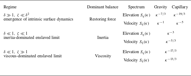
 Sη(κ)
 Sη˙(κ)
 ζ≪1
 ζ≫1

 a
 b
 c
 C(rx+Uintτ,τ)=⟨η(x,z;t)η(x+rx+Uintτ,z;t+τ)⟩/⟨η(x,z;t)η(x,z;t)⟩
 rx
 τ
 Uint
 C
 d
 e
 f
 Sη∼κx−15/4
 Sη˙∼κx−3/4

 a
 b

 Sηmax
 κmax
 Sηmax
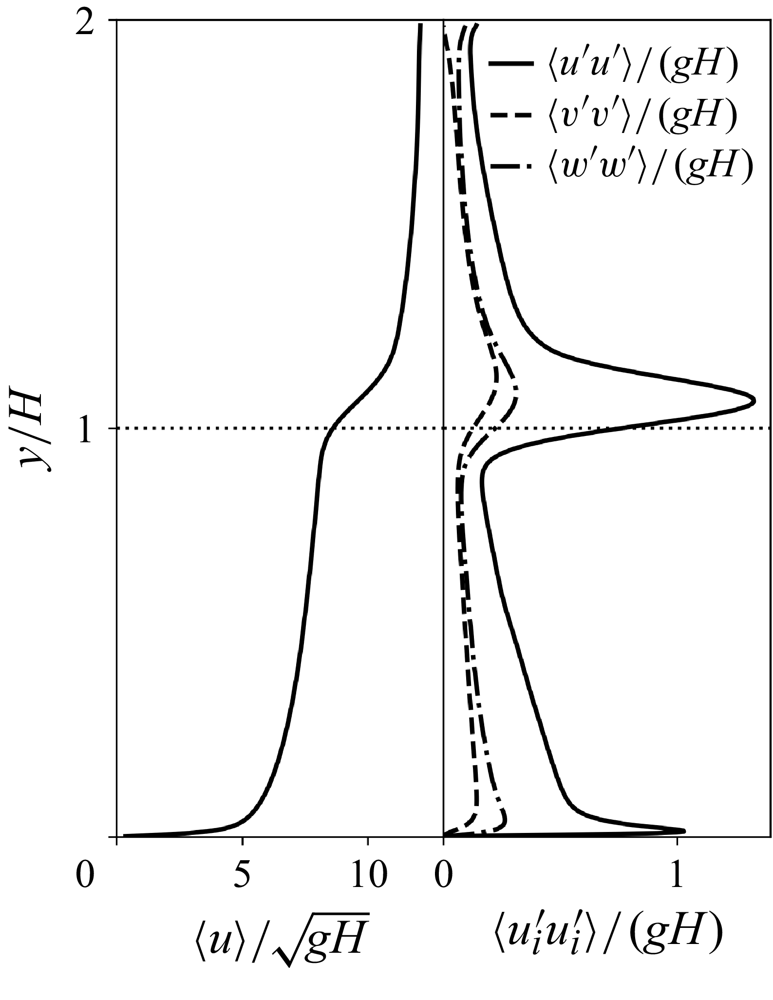
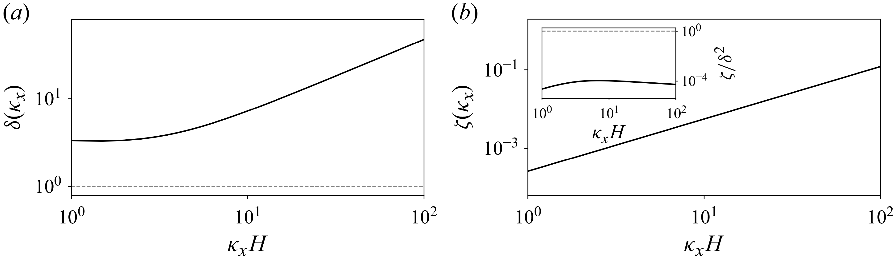
 δ=ω0/ωt>1
 ζ=γ/ωt≪δ2
 κx


