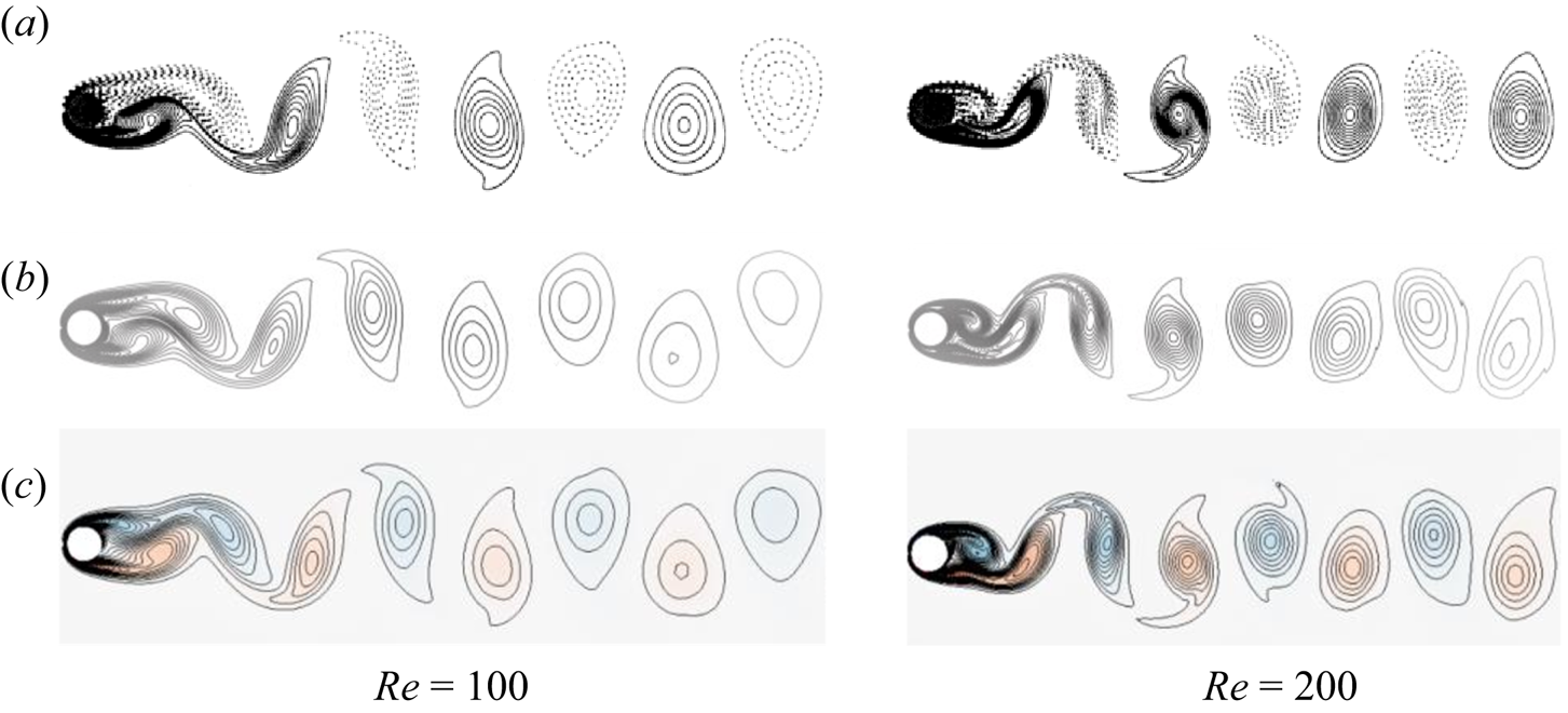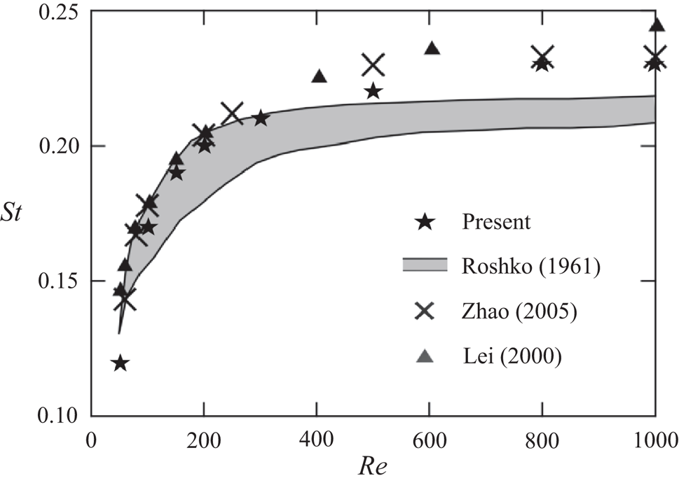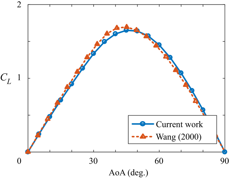

1. Introduction
Fluid flows can be very complex in simple configurations, and the interaction between fluid and structures or the presence of reconfigurable boundaries can further complicate the problem. The nonlinear nature and multiple time scales involved in these problems make it challenging to analyse and dissect the dynamic characteristics of the system (Bazilevs, Takizawa & Tezduyar Reference Bazilevs, Takizawa and Tezduyar2013). In recent years, modal decomposition techniques have shown the potential for extracting critical flow structures from the complex flow fields. However, there are several mathematical and formulation challenges that should be overcome before adopting these techniques to study the flow dynamics of reconfigurable systems. This is the main focus of this paper.
Modal decomposition is a branch of methods that aim to highlight energetically or dynamically significant features of data (Taira et al. Reference Taira, Brunton, Dawson, Rowley, Colonius, McKeon, Schmidt, Gordeyev, Theofilis and Ukeiley2017). Modal analysis methods have been proposed for different purposes in the past decade, including identifying the linear modal representation of complicated flows. The spatial modes extracted from the flow field, along with their characteristic temporal values, can be used to pinpoint important dynamics, build reduced-order models or develop control strategies. Some modal analysis methods involve discretizing the governing equations to examine the stability of the system (McKeon, Sharma & Jacobi Reference McKeon, Sharma and Jacobi2013; Jeun, Nichols & Jovanović Reference Jeun, Nichols and Jovanović2016). Modal analysis methods serve a critical role in modern fluid dynamics research and have been continuously evolving for more challenging problems. Further details can be found in many books and review papers, just to name a few here: Ukeiley et al. (Reference Ukeiley, Cordier, Manceau, Delville, Glauser and Bonnet2001), Theofilis (Reference Theofilis2011), Holmes et al. (Reference Holmes, Lumley, Berkooz and Rowley2012) and Kutz (Reference Kutz2013), etc.
Two of the most popular modal analysis tools, proper orthogonal decomposition (POD) and dynamic mode decomposition (DMD), share the same characteristic of being data-driven. They both do not need governing equations and are applicable to various disciplines. However, the lack of spatial recognition of the boundaries in these methods poses a problem when they are applied to the problems with moving or deforming geometries. Their spatial modes should be embedded onto a fixed Eulerian space to provide physical representation. However, in many problems, including fluid–structure interaction (FSI) problems, fluid motion often is coupled to deforming or/and vibrating bodies where the geometry is continuously changing. Under such circumstances, without employing a unique geometrical description, the application of the data-driven modal analysis methods is restrained. Different approaches have been proposed to solve this issue.
The fluid-only approaches, wherein the modal analysis is used only within the fluid domain, have been applied to the flow past a pitching foil (Mariappan et al. Reference Mariappan, Gardner, Richter and Raffel2013) or a flexible cantilever beam (Cesur et al. Reference Cesur, Carlsson, Feymark, Fuchs and Revstedt2014). It is also utilized to extract the modal content of the wake behind a flexible membrane in experiments (Schmid Reference Schmid2010). Similar techniques are proposed for the structural response and were employed to identify the characteristic pattern of a flapping fish pectoral fin (Bozkurttas et al. Reference Bozkurttas, Mittal, Dong, Lauder and Madden2009) and a waving flag (Michelin, Smith & Glover Reference Michelin, Smith and Glover2008). Although the most important features of structure or fluid are revealed with these methods, the connection between them is not captured. To understand the correlation between the two domains, some research includes both fluid and solid dynamics in the modal analysis. For example, Goza & Colonius (Reference Goza and Colonius2018) used the combined energy of the fluid and structural phases in constructing POD modes and group the responses of the fluid and structure into a single dataset and employ the DMD technique on them. Liberge & Hamdouni (Reference Liberge and Hamdouni2010) computed the POD modes by interpolating the time-variant grid to a fixed uniform grid to form a global velocity field. Tadmor et al. (Reference Tadmor, Bissex, Noack, Morzynski, Colonius and Taira2008) leveraged the known periodicity of the system to partition the data and extract the physical harmonic modes. Menon & Mittal (Reference Menon and Mittal2020a) performed DMD to a pitching rigid airfoil by a change of reference frame. However, when these methods are applied to systems involving deforming and/or moving volumetric bodies, certain restrictions are encountered, like the representation of moving interfaces between the fluid and solid requires an infinite number of modes, or the system exhibits non-periodic dynamics preventing the use of any prior knowledge.
Moreover, in many FSI systems, the structural response consists of a few fundamental modes, while the flow response is made up of many dynamically important modes and hidden variables (Blevins Reference Blevins1977; Saffman Reference Saffman1992; Eldredge Reference Eldredge2019). The interaction between fluid and solid can persist even at a very small deflection limit of their interfaces. In this situation, the coupled system can be linearized around the mean interface, and the dynamic interactions between two phases can be captured with Eulerian linear models. Still, there exists another mode of interaction that is accompanied by large changes in the geometry of the solid. This mode interaction is more abundant in the systems with large deformation and extensive reconfiguration capabilities such as flag vibration, bird and insect wings, or fish fins. In many of these systems, repositioning of the interface results in new flow conditions and substantial changes in the interaction forces between the fluid and structure. In this case, to represent the flow with a linear combination of modes, it is necessary to incorporate the geometry changes of the flow domain in the modal analysis and essentially map the problem to a domain with fixed interfaces and bring the effect of mapping function into the governing equations of flow and structure.
In this paper we propose a novel method to combine the conformal mapping technique with the modal analysis. An arbitrary smooth geometry is transformed into a fixed geometry through a unique invertible mapping that preserves many important properties of the flow (Pozrikidis Reference Pozrikidis2011; Eldredge Reference Eldredge2019). Conformal mappings preserve angles and form a systematic framework to perform shape analysis of deformable surfaces. They are simple, efficient, energy-invariant and mathematically well-understood procedures with infinitely many derivatives. We focus on two-dimensional systems and express the flow equations based on the vorticity-stream function form in the transformed domain to obtain the flow field on a canonical planar domain for the subsequent data-driven modal analysis. This method provides a natural mapping (as a model of geometric group theory) between a canonical geometry and the real geometry and is applicable to a broad class of smooth geometry. Through examples, the benefit of this method will be shown in the later sections.
The rest of this paper is as follows. In § 2 we first provide an introduction to POD and DMD. We discuss how the proposed method can overcome modal analysis limitations for systems with shape-changing bodies. In § 3 different examples with deforming surfaces are examined to demonstrate how the proposed method can be applied to identify significant flow features. Finally, the conclusion and future direction will be given in § 4.
2. Methodology
The basics of the two most popular modal analysis techniques, POD and DMD, will be introduced first. Both of these methods are data-driven and are widely used for various applications. We introduce the proposed method aiming to enable the modal analysis of systems with deforming/moving geometries. The limitations of the proposed method will be reviewed at the end.
2.1. Proper orthogonal decomposition
The proper orthogonal decomposition technique, also known as the principal component analysis and Karhunen–Loeve transformation, optimally decomposes a complex system into linear combinations of modes. The orthogonal spatial modes acquired from the POD technique capture the most disturbance energy of the flow. Proper orthogonal decomposition was introduced to analyse flow problems first by Lumley (Reference Lumley1967), and since then, it has been one of the popular techniques for analysing diverse flow fields. It has numerous applications including but not limited to reduced-order modelling (Aubry et al. Reference Aubry, Holmes, Lumley and Stone1988; Noack et al. Reference Noack, Afanasiev, Morzyński, Tadmor and Thiele2003; Rowley, Colonius & Murray Reference Rowley, Colonius and Murray2004), flow control (Ravindran Reference Ravindran2000; Afanasiev & Hinze Reference Afanasiev, Hinze, Polis, Cagnol and Zolésio2001) and design optimization (LeGresley & Alonso Reference LeGresley and Alonso2000).
The purpose of POD is to form a group of deterministic functions  $\phi _i(z)$ that is most similar to the members of a sample function
 $q(z)$, with
 $z$ representing the embedded coordinate of the field (Lumley Reference Lumley1967). The notion of ‘most similar’ is defined by maximizing the cosine similarity quantity of
 \begin{equation} \frac{\langle q,\phi\rangle}{\|\phi\|_2 \|\phi\|_2}. \end{equation}
Here the parenthesis  $\langle \,,\rangle$ denotes the inner product
 $\langle f,g \rangle =\int _{\varOmega } f^*(x) g(x)\,{\textrm {d}x}$, where the asterisk superscript represents both the complex conjugate of a complex scalar and the Hermitian transpose of a vector or tensor, and
 $\|\cdot \|$ denotes the Euclidean 2-norm. When this normalized inner product is maximized, the function
 $\phi$ is nearly parallel to a particular characteristic feature of the field
 $q$. The necessary condition for the optimal linear representation is that
 $\phi$ should be an eigenfunction of the eigenproblem
 \begin{equation} \int_{\varOmega}\langle q(z), q(z') \rangle \phi(z')\,\textrm{d}z' =\lambda\phi(z). \end{equation}
Since  $R(q(z), q(z'))=\langle q(z), q(z')\rangle$ is compact and bounded, the Hilbert–Schmidt theory guarantees that the eigenproblem has a solution (Lumley Reference Lumley1967). The eigenmodes
 $\phi _i$ can be ranked according to their eigenvalues
 $\lambda _i \geq 0$, guaranteed to be larger than
 $0$ due to the non-negative definiteness of
 $R(q(z), q(z'))$. The eigenvectors are orthogonal and provide complete bases for representing
 $q$.
For fluid problems, POD is usually applied to the fluctuation of the flow quantities. In the current work we adopt the snapshot POD variant proposed by Sirovich (Reference Sirovich1987) for its efficiency in handling very high-dimensional problems often encountered in computational fluid dynamics problems. The flow field  $u$ is decomposed into spatial modes
 $\phi _i(\boldsymbol {x})$ and temporal coefficients
 $a_i(t)$, i.e.
 \begin{equation} u(\boldsymbol{x}, t)=\bar{u}(\boldsymbol{x}) + u'(\boldsymbol{x},t)=\bar{u}(\boldsymbol{x})+\sum_{i=1}^{N} a_i(t)\phi_i(\boldsymbol{x}), \end{equation}
where  $(\bar {{A}})$ denotes the time-averaging operation. The procedure of applying snapshot POD to a discrete dataset is explained below. For a discrete dataset with
 $m$ snapshots, the data matrix of
 $\boldsymbol {U}=\{\boldsymbol {u'}_1, \boldsymbol {u'}_2 ,\ldots , \boldsymbol {u'}_m\}$ is formed by stacked together
 $\boldsymbol {u'}_i$, the discrete flow disturbance data of the
 $i$th snapshot, into a
 $n\times 1$ vector. The data could be the flow velocity, vorticity or any other quantity of interest. Since
 $\boldsymbol {U}\boldsymbol {U}^{\textrm {T}}$ and
 $\boldsymbol {U}^{\textrm {T}}\boldsymbol {U}$ have the same set of non-zero eigenvalues, the data structure is examined to decide which combination is a better choice for the eigenvalue calculation. In modern flow applications, the dimension of the acquired dataset from either numerical simulation or an experimental particle image velocimetry system is usually much larger than the number of snapshots. Therefore, oftentimes, it is reasonable to select the covariance matrix as
 $\boldsymbol {U}^{\textrm {T}}\boldsymbol {U}$ instead, and solve the eigenvalue problem of
 \begin{equation} \boldsymbol{U}^{\textrm{T}}\boldsymbol{U}\boldsymbol{W}\psi_j=\lambda_j\psi_j, \quad \psi_j\in\mathbb{R}^m, \quad m\ll n. \end{equation}
The matrix  $\boldsymbol {W}$ here is a weighting matrix accounting for the numerical quadrature and can be constructed for different purposes (Schmidt & Colonius Reference Schmidt and Colonius2020).
The POD modes,  $\phi _j$, are defined as the eigenvector of the covariance matrix
 $\boldsymbol {U}\boldsymbol {U}^{\textrm {T}}$, and are related to
 $\psi _j$ by
 \begin{equation} \phi_j=U\psi_j\frac{1}{\sqrt{\lambda_j}}\in\mathbb{R}^n, \quad j=1,2,\ldots,m, \end{equation}
where the eigenvalues  $\lambda _j$ represent the energy level of the corresponding POD modes,
 $\phi _j$. The more popular choices in the flow data are velocity or vorticity, which POD modes are selected based on their physical representation of the kinetic energy or enstrophy of the flow, respectively. Note that this procedure is essentially equivalent to executing a singular value decomposition (SVD) on the data matrix
 $\boldsymbol {U}$, with the left-singular matrix containing the orthonormal POD modes. The temporal coefficients can be obtained from
 \begin{equation} a_j=\boldsymbol{U}^{\textrm{T}}\phi_j, \quad a_j\in\mathbb{R}^m. \end{equation}
The reconstruction of the snapshots can be performed with a truncated set of POD modes. A simple criterion for deciding the number of required modes  $p$ is based on their cumulative representation of the energy or enstrophy, or equivalently, when
 $\sum _{i=1}^{p} \lambda _i\sim 1$. The truncation of the lower-energy modes are equivalent to denoising the signal, a technique which is extensively used in the fields of signal processing, estimation and pattern recognition (Ly & Tran Reference Ly and Tran2001; Lanata & Del Grosso Reference Lanata and Del Grosso2006; Astrid et al. Reference Astrid, Weiland, Willcox and Backx2008). The reconstructed snapshots can be recovered by
 \begin{equation} \tilde{u}_j(t)=\sum_{j=1}^{p} a_j(t)\phi_j . \end{equation}
Proper orthogonal decomposition modes have several important and unique advantages. They are orthogonal to each other and encode unique aspects of the flow, which is beneficial for constructing an efficient reduced-order model for various flow configurations. Another advantage is that POD distributes the energy of the non-noise part of the signal into the leading POD modes with coherent structures, and, hence, equivalently increases the signal-to-noise ratio. Numerous extensions of the POD technique are developed to overcome different practical and computational challenges. We will introduce some of them that are relevant to the proposed work later in § 2.3.
2.2. Dynamic mode decomposition
Dynamic mode decomposition, first proposed by Schmid (Reference Schmid2010), is another popular and widely used flow analysis technique. It produces a set of spatial modes with corresponding characteristic frequencies and growth/decay rates. The idea behind DMD is to identify the linear harmonic modes which disclose distinct dynamics of a nonlinear system through the eigendecomposition of a best-fit linear operator. The data matrix, defined as  $\boldsymbol {U}=\{\boldsymbol {u}_1, \boldsymbol {u}_2,\ldots , \boldsymbol {u}_m\}$, is partitioned into two time-consecutive sets
 $\boldsymbol {U}_{1:m-1}=\{\boldsymbol {u}_1, \boldsymbol {u}_2,\ldots ,\boldsymbol {u}_{m-1}\}$ and
 $\boldsymbol {U}_{2:m}=\{\boldsymbol {u}_2, \boldsymbol {u}_3,\ldots ,\boldsymbol {u}_m\}$. Dynamic mode decomposition seeks to find a constant transition matrix
 $\boldsymbol {A}$ such that
 $\boldsymbol {U}_{2:m} \approx \boldsymbol {A}\,\boldsymbol {U}_{1:m-1}$, subject to minimizing the cost function
 \begin{equation} C=\sum_{i=1}^{m-1} \|\boldsymbol{u}_{2,i}-\boldsymbol{A}\,\boldsymbol{u}_{1,i}\|^2, \end{equation}
where  $\boldsymbol {u}_{1,i}$ and
 $\boldsymbol {u}_{2,i}$ are the
 $i$th columns of the matrices
 $\boldsymbol {U}_{1:m-1}$ and
 $\boldsymbol {U}_{2:m}$, respectively. The unique minimum-norm solution of this problem based on the Frobenius norm of
 $\boldsymbol {A}$ is
 \begin{equation} \boldsymbol{A}= \boldsymbol{U}_{2:m} \, \boldsymbol{U}_{1:m-1}^+ , \end{equation}
where  $\boldsymbol {U}_{1:m-1}^+=(\boldsymbol {U}_{1:m-1}^*\,\boldsymbol {U}_{1:m-1})^{-1}\boldsymbol {U}_{1:m-1}^*$ is the Moore–Penrose left inverse of the matrix
 $\boldsymbol {U}_{1:m-1}$. The eigenvectors of
 $\boldsymbol {A}$ are defined as the DMD modes, where the frequencies and growth/decay rates are determined from the imaginary and real parts of the eigenvalues.
A computationally efficient technique to calculate DMD modes is introduced by Schmid (Reference Schmid2010). This technique is used in this paper. Here, the first step is to compute the reduced SVD of the data matrix
 \begin{equation} \boldsymbol{U}_{1:m-1}=\boldsymbol{S}\,\boldsymbol{\varSigma}\,\boldsymbol{ V}^*, \end{equation}
where  $\boldsymbol {S}$ is the left-singular matrix,
 $\boldsymbol {\varSigma }$ is the singular value matrix and
 $\boldsymbol {V}$ is the right-singular matrix. We then define the function
 \begin{equation} \boldsymbol{B}\,\equiv\, \boldsymbol{S}^*\,\boldsymbol{U}_{2:m}\,V\,\boldsymbol{\varSigma}^{-1} \end{equation}
and solve the eigenproblem of
 \begin{equation} \boldsymbol{B}\,\tilde{\omega}_j \,=\, \tilde{\mu}_j \,\tilde{\omega}_j \end{equation}
to find the DMD modes as
 \begin{equation} \tilde{\psi}_j \,=\,\boldsymbol{S}\, \tilde{\omega}_j. \end{equation}
The modes  $\tilde {\psi }_j$ and eigenvalues
 $\tilde {\mu }_j$ are acquired from matrix
 $\boldsymbol {B}$ and are related to that acquired from using matrix
 $\boldsymbol {A}$ with
 \begin{equation} \psi_j=\tilde{\mu}_j^{-1}\, \boldsymbol{U}_{2:m} V \varSigma^{-1}\, \tilde{\omega}_j, \quad \mu_j=\frac{\textrm{log}(\tilde{\mu}_j)}{\delta t} , \end{equation}
where  $\delta t$ is the time separation between two consecutive snapshots (Tu et al. Reference Tu, Rowley, Luchtenburg, Brunton and Kutz2014).
Each DMD mode is a spatial mode indicating a distinct dynamic of the system. These modes are equivalent to a finite-dimensional approximation of the Koopman operators (Rowley et al. Reference Rowley, Mezić, Bagheri, Schlatter and Henningson2009; Mezić Reference Mezić2013), which map a nonlinear system to an infinite-dimensional linear system. The DMD technique, as Schmid (Reference Schmid2010) points out, is not limited to temporal but can also be spatial stability analyses through rearranging the data matrix along the spatial axis of interest.
If the  $j$th mode obtained from the DMD approach has a corresponding eigenvalue
 $\tilde {\mu }_j$, then the frequency and growth/decay rate of this mode can be calculated from
 \begin{equation} f_j=\frac{\text{ang}\left(\tilde{\mu}_j\right)}{2{\rm \pi}\,\delta t}, \quad d_j=\frac{\log|\tilde{\mu}_j|}{\delta t}, \end{equation}
where the ang( $\tilde {\mu }_j$) is the phase angle of the complex eigenvalue
 $\tilde {\mu }_j$. The low-rank projected solution can be reconstructed at any time with
 \begin{equation} \boldsymbol{u}_{DMD} (t)=\sum_{k=1}^{K} b_k(0)\, \psi_k\, \textrm{e}^{\mu_j t}, \end{equation}
where  $K$ is the rank of the reduced SVD approximation to
 $\boldsymbol {U}_{1:m-1}$ and
 $b_k(0)$ is the initial amplitude of the
 $k$th mode. The above equation can be represented in matrix form as
 \begin{equation} \boldsymbol{u}_{DMD} (t)=\boldsymbol{\varPsi}\, \text{diag}(\textrm{e}^{\mu_j t})\,\boldsymbol{b}, \end{equation}
where  $\boldsymbol {\varPsi }$ is the matrix formed from the DMD modes
 $\psi$,
 $\text {diag}(\textrm {e}^{\mu _j t})$ is a diagonal matrix with
 $\textrm {e}^{\mu _j t}$ as entries and
 $\boldsymbol {b}$ is a vector calculated by
 \begin{equation} \boldsymbol{b} = \boldsymbol{\varPsi}^+ x_1, \end{equation}
where  $x_1$ is the initial snapshot and
 $\boldsymbol {b}$ is a vector formed from
 $b_k(0)$.
The above algorithm is one of the common definitions of DMD modes. As Tu et al. (Reference Tu, Rowley, Luchtenburg, Brunton and Kutz2014) point out, there are multiple different definitions of DMD modes and each definition provides a different perspective of the system dynamics. Dynamic mode decomposition is capable of isolating specific dynamics in the system according to their frequencies. It is data-driven and can be expanded with mathematical tools for numerous applications. Compared with POD, DMD modes are not orthogonal to each other and have no differentiation in eigenvalue importance, but they can reveal critical dynamic information of the system.
2.3. Geometrically weighted modal decomposition
The commonly used snapshot POD and classical DMD both produce spatial Eulerian modes, whereas the temporal effects are incorporated in their temporal coefficients or eigenvalues. Different variants of the POD and DMD methods have been proposed to expand the capabilities of these methods (Holmes et al. Reference Holmes, Lumley, Berkooz and Rowley2012; Kutz Reference Kutz2013; Taira et al. Reference Taira, Brunton, Dawson, Rowley, Colonius, McKeon, Schmidt, Gordeyev, Theofilis and Ukeiley2017).
One of the usual difficulties of the popular snapshot POD is that while their resultant modes are energetically optimal, they might fail to capture critical system dynamics. The spectral POD proposed by Towne, Schmidt & Colonius (Reference Towne, Schmidt and Colonius2018) finds modes that depend on both space and time by extending the stochastic ensemble from snapshots of a flow field to a collection of realizations of the time-dependent flow. Another method with the same name (Sieber, Paschereit & Oberleithner Reference Sieber, Paschereit and Oberleithner2016) applies a filter to the correlation matrix such that the stochastic fluctuations are attenuated while leaving the coherent structures unaffected. The sequential POD (Jørgensen, Sørensen & Brøns Reference Jørgensen, Sørensen and Brøns2003) collect multiple sets of snapshots with different parameter settings to ensure that the dynamically important data are better represented in the extracted modes. Also, POD techniques have been extended to incorporate available information about the importance of modes as a weighting function in Bayesian methods such as the probabilistic principle component analysis (PCA) (Tipping & Bishop Reference Tipping and Bishop1999) or sensible PCA (Moghaddam & Pentland Reference Moghaddam and Pentland1995; Roweis Reference Roweis1998).
Modified DMD methods have been developed to improve certain shortcomings of the classical DMD approach. For example, the streaming DMD (Hemati, Williams & Rowley Reference Hemati, Williams and Rowley2014) can update the DMD computations incrementally with a number of orthogonal basis vectors, windowed DMD (Zhang et al. Reference Zhang, Rowley, Deem and Cattafesta2019) permits the frequency change in the system by placing less weight on older snapshots, and multiresolution DMD (Kutz, Fu & Brunton Reference Kutz, Fu and Brunton2016) recursively isolates the lower-rank modes of the system to separate the important dynamics with distinct scales.
However, lots of FSI systems such as fish swimming (Liu, Wassersug & Kawachi Reference Liu, Wassersug and Kawachi1996), flapping wings (Takizawa et al. Reference Takizawa, Henicke, Puntel, Spielman and Tezduyar2012), heart valves (Kamensky et al. Reference Kamensky, Hsu, Schillinger, Evans, Aggarwal, Bazilevs, Sacks and Hughes2015) or wind turbines (Hsu & Bazilevs Reference Hsu and Bazilevs2012) have moving or deforming volumetric structures with large deformation. As most of the modal analysis techniques are data-driven, their spatial description must remain time invariant for the modes to capture physically significant features of the flow. When there is a large deformation body in the flow, immersed interface techniques (Mittal & Iaccarino Reference Mittal and Iaccarino2005) with a fixed grid or a body-fitted time-varying coordinate system (Connell & Yue Reference Connell and Yue2007) can be employed to study the flow dynamics computationally. In the former group, to capture the moving interface, an infinite number of modes are needed, akin to how infinite Fourier modes are required to rebuild a step function. For the latter case, the spatial modes acquired from the modal analysis do not have a fixed spatial grid to embed on and are hence uninterpretable. Suppose the data-driven techniques like POD and DMD are to be employed to understand the flow physics in these applications, in that case, a mathematical framework is necessary for efficiently and accurately transforming a time-variant fluid domain into a time-invariant one with minimal changes to the flow equations. The proposed geometrically weighted modal decomposition techniques combine a proper transformation and the modal analysis to tackle the spatial embedding problem.
2.3.1. Conformal mapping and body-fitted grids
To describe the fluid dynamics around a moving and deforming structure, we employ a body-fitted mesh and the finite difference approach. The grid is generated with a well-established conformal mapping technique (Pozrikidis Reference Pozrikidis2011; Eldredge Reference Eldredge2019), which can be deployed upon any arbitrary smooth shape to transform the geometry into a canonical shape, e.g. a cylinder with a specified diameter. The choice of the transformation is a critical aspect of calculating the physically relevant geometric weighting function for the modal analysis procedures.
We assume that the shape of an arbitrary object can be represented with a series of sufficiently smooth contour curves in the Cartesian space. The procedure, following Pozrikidis (Reference Pozrikidis2011), is as follows.
(i) The contour boundary of the body is traced with
 $N$ points. The coordinates of the points are represented as ${z_j=x_j+\textrm {i} y_j}$ numbered in the counterclockwise direction for $j=1,\ldots ,N$.
(ii) Here we choose to map the exterior of the body to the exterior of a circle with the radius
$\lambda$ centred at the origin. The computational grid is constructed based on the cylindrical coordinate around the circle defined as $\zeta =\lambda \textrm {e}^{\textrm {i}\,\phi }$, with $\phi$ being the polar angle. The relation between $\lambda$, $\phi$ and $z$ can be expressed with the Laurent series expansion
(2.19)\begin{equation} z(\phi)=\lambda \textrm{e}^{\textrm{i}\phi}+a^0+\sum_{n=1}^{\infty} a^n \textrm{e}^{-\textrm{i} \,n\phi}. \end{equation}(iii) The radial distance
$\lambda$ and the series coefficients $a^n$ are calculated with the use of the orthogonality properties of $\textrm {e}^{-\textrm {i}\,n\phi }$ kernel,
(2.20)\begin{gather} \lambda = \frac{1}{2{\rm \pi}}\int_{0}^{2{\rm \pi}} [x(\phi)\cos(\phi)+y(\phi)\sin(\phi)]\,\textrm{d}\phi, \end{gather}(2.21)\begin{gather}\text{Re}[a^n] = \frac{1}{2{\rm \pi}}\int_{0}^{2{\rm \pi}} [x(\phi)\cos(n\phi)-y(\phi)\sin(n\phi)]\,\textrm{d}\phi, \end{gather}(2.22)\begin{gather}\text{Im}[a^n] = \frac{1}{2{\rm \pi}}\int_{0}^{2{\rm \pi}} [x(\phi)\sin(n\phi)+y(\phi)\cos(n\phi)]\,\textrm{d}\phi. \end{gather}(iv) The coordinates
$z(\phi )$ are expressed on the Cartesian plane for selected values of $\lambda$ and $\phi$, and compared with the original contour curve. The values $\phi _i$ are then optimized through minimization of $L^2$-norm of the error,
(2.23)\begin{equation} \|\Delta z_i\|^2=(x_i-x(\phi_i))^2+(y_i-y(\phi_i))^2. \end{equation}


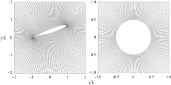
As an example, the conformal grid for an energy efficient transport (EET) high-lift airfoil with an attached flap generated from this algorithm along with the cylindrical grid in  $\zeta$ plane are shown in figure 1. The grid is also strained logarithmically in the radial direction with more resolution near the surface to accurately capture the unsteady aerodynamic effects.
Computational grid in the physical domain around an EET high-lift airfoil and the transformed domain around a unit circle.

The most important advantage of this procedure for the modal decomposition is that the transformed domain in the  $\zeta$-plane is time invariant. In general, the computational grid of the transformed domain is designed to resolve the space where most dynamics happen, or where the geometry has its most temporal variations. The conformal mapping mainly expands the region next to the surface where fine flow details are present and, thus, results in better identification of such flow features. Note that the conformal mapping process does not change the value of the independent variables embedded in the spatial grid; thus, the mapping effectively redistributes the independent variables in space. In this paper, the distribution of the points along the contour curve is determined by the local surface curvature. The technique also sets up the fixed grid required for POD, DMD and other spatial modal decomposition methods. More discussion about this aspect will be given later in this section.
2.3.2. Governing flow equations
The flow dynamics around the structure is solved in the transformed domain  $\zeta =r \textrm {e}^{\textrm {i}\,\phi }$ using the modified Navier–Stokes equation incorporating the effect of the conformal transformation. The Navier–Stokes equations are expressed in the vorticity-stream function
 $(\omega -\psi )$ form as
 \begin{gather} \frac{\partial\omega}{\partial t}+\frac{1}{\sqrt{|J|}}\left[v_r\frac{\partial\omega}{\partial r}+\frac{v_\theta}{r}\frac{\partial\omega}{\partial\theta}\right]=\frac{1}{Re \, |J|}\left[\frac{\partial^2\omega}{\partial r^2}+\frac{1}{r} \frac{\partial \omega}{\partial r}+\frac{1}{r^2}\frac{\partial^2\omega}{\partial\theta^2}\right], \end{gather}
 \begin{gather} \frac{\partial^2\psi}{\partial r^2}+\frac{1}{r}\frac{\partial\psi}{\partial r}+\frac{1}{r^2}\frac{\partial^2\psi}{\partial\theta^2}=-|J|\omega, \end{gather}
where  $Re$ is the Reynolds number,
 $|J|$ is the determinant of the Jacobian of the transformation
 $\zeta =\xi +\textrm {i}\eta \Rightarrow z=x+\textrm {i} y$, and
 $v_r$ and
 $v_\theta$ are the transformed velocities which incorporate time-dependent effects of the mapping process. Because the independent variables like the vorticity do not change during the conformal mapping process, we can recover the desired flow data with the reverse mapping from the solution obtained in the transformed domain. A similar procedure using Joukowski transformation can be found in Guglielmini & Blondeaux (Reference Guglielmini and Blondeaux2004) and Zhu & Peng (Reference Zhu and Peng2009). Further detail of the formulation is provided in appendix B.
2.3.3. Fluid–structure interaction
Aside from the geometry change, the current algorithm also embodies the translational and rotational motions of the structure, denoted with the heaving distance  $h$ and pitching angle
 $\alpha$, respectively. For the FSI problem in § 3.3, the body motion is modelled by connecting the structure to a set of linear and torsional dampers and springs with damping and stiffness coefficients
 $c_{h/\alpha }$ and
 $k_{h/\alpha }$, respectively. The structural motions are related to the fluid forces and torques by the equations of motion
 \begin{align} \left[ \begin{array}{@{}cc@{}} m & S_\alpha \\ S_\alpha & I \end{array} \right] \left[ \begin{array}{@{}c@{}} \ddot{h} \\ \ddot{\alpha} \end{array} \right] + \left[ \begin{array}{@{}cc@{}} c_h & 0 \\ 0 & c_\alpha \end{array} \right] \left[ \begin{array}{@{}c@{}} \dot{h} \\ \dot{\alpha} \end{array} \right] + \left[ \begin{array}{@{}cc@{}} k_h & 0 \\ 0 & k_\alpha \end{array} \right] \left[ \begin{array}{@{}c@{}} h \\ \alpha \end{array} \right] = \left[ \begin{array}{@{}c@{}} F_{fluid} \\ M_{fluid} \end{array} \right], \end{align}
where  $m$ is the mass of the body and
 $S_\alpha$ and
 $I$ are the static imbalance and moment of inertia, respectively.
The fluid and the structural equations are solved using a tightly coupled algorithm with the following steps.
(i) At time step n, the heaving motion
$\dot {h}_{n-1}$ and pitching motion $\dot {\alpha }_{n-1}$ from the last time step are used as the initial values for solving FSI problem at time $n$.(ii) The hydrodynamic forces and moment are calculated based on the current value of
$\dot {h}$ and $\dot {\alpha }$.(iii) We update
$\dot {h}_n$ and $\dot {\alpha }_n$ with the calculated hydrodynamic forces and moment exerted on the airfoil.(iv) The iteration between the fluid and foil dynamics repeats until
$\dot {h}_n$ and $\dot {\alpha }_n$ converge, then the algorithm progresses to the next time step.


The Navier–Stokes equations are discretized in  $r$,
 $\theta$ and
 $t$. For the vorticity transportation equation, a central difference scheme with second-order accuracy is implemented. For time integration, the vorticity field is updated at each time step via an alternative direction implicit technique. Two boundary conditions are imposed: on the structure surface, the no-slip boundary condition is enforced, and the free stream velocity is specified at the far-field boundaries. The Poisson equation is solved using a semi-spectral method, wherein the Fourier transformation is employed along
 $\theta$, and the finite difference technique is used along
 $r$. The validation of the algorithm is presented in appendix A.
2.3.4. Modal analysis
The algorithm introduced above is capable of modelling the flow dynamics of a system with arbitrary smooth shape-changing bodies. Through the conformal mapping procedure, the system now resides on a time-invariant grid. This resolves the aforementioned problem of spatial recognition when applying classical modal analysis techniques to FSI systems involving a deforming/moving volumetric body. The conformal mapping enables the modal analysis to be applied to such a system by weighting the spatial distribution of the flow data based on the geometry in the physical domain and, thus, is named as geometrically weighted modal decomposition (GW-MD). However, since the conformal mapping process transforms the time-dependent structural domain to a fixed shape, the modes obtained from GW-MD are now spatio-temporal modes. Some questions arising from this procedure would be: what temporal effects have been incorporated in these modes? How does the transformation change the POD or DMD modes, and how should we interpret them? We will discuss these questions next.
First, let us consider how the mapping process changes the physical properties of the modes. In the transformed  $\zeta$ domain, the grid is time invariant, and we can employ modal analysis techniques to get the spatial modes. When an inverse mapping is applied to project the modes to the original
 $z$ domain, temporal effects are introduced through the Jacobian
 $\boldsymbol {J}$ of
 $\zeta =\xi +\textrm {i}\eta \Rightarrow z=x+\textrm {i}y$ transformation, with the metric of the transformation being
 \begin{equation} |J|(t)=\frac{\partial x(t)}{\partial \xi}\frac{\partial y(t)}{\partial \eta}-\frac{\partial x(t)}{\partial \eta}\frac{\partial y(t)}{\partial\xi}, \end{equation}
wherein the  $x$ and
 $y$ are the time-varying physical position of a particular point in the physical domain. Therefore, the Jacobian is also time variant. It follows that
 \begin{equation} \textrm{d}\vec{z} = |J|\, \textrm{d}\vec{\zeta} \quad \text{and} \quad \boldsymbol{\nabla}_{z}=\boldsymbol{J}^{-1} \boldsymbol{\cdot} \boldsymbol{\nabla}_{\zeta}, \end{equation}
and based on the mapping properties,
 \begin{equation} \boldsymbol{J}^{-1}=\frac{1}{|J|} \boldsymbol{J}^{\textrm{T}}. \end{equation}
The Jacobian serves as a spatial weighting originating from the conformal mapping procedure; hence, called the geometric weighting. To illustrate how this weighting affects the outcome of the POD modes, we take the velocity and vorticity as examples. From (2.2) we know that the POD modes are the solution to the eigenproblem. This inner product in the transformed domain  $\varOmega _{\zeta }$ defines how the geometric mapping affects the modes.
(i) Velocity: the inner product of the velocity in the physical and transformed domains are related through
 \begin{align} R(v,v) & = \langle v, v \rangle = \int_{\varOmega_\zeta} v^*(z) v(z) \,\textrm{d}\zeta = \int_{\varOmega_\zeta} (\boldsymbol{\nabla}_\zeta \times \psi)^* (\boldsymbol{\nabla}_\zeta \times \psi)\,\textrm{d}\zeta\nonumber\\ & = \int_{\varOmega_z} (\boldsymbol{J}\boldsymbol{\cdot} \boldsymbol{\nabla}_z \times \psi)^* (\boldsymbol{J}\boldsymbol{\cdot} \boldsymbol{\nabla}_z \times \psi) \frac{1}{|J|}\,\textrm{d}z = \int_{\varOmega_z} (\boldsymbol{\nabla}_z \times \psi)^* (\boldsymbol{\nabla}_z \times \psi) \,\textrm{d}z. \end{align}
The conformal transformation hence preserves the kinetic energy. This is because of a specific relation between the role of mapping on the dilatation term and gradient operator. As a result, for stationary objects, modes acquired in the transformed domain are the exact modes obtained in the physical domain based on the kinetic energy. We should emphasize that currently there is no proper way to perform POD in the actual physical domain due to the moving structures. Through the conformal mapping we merge the structural effect into the governing equation and the POD modes acquired in the transformed domain incorporate the solid movement into the flow. Geometrically weighted proper orthogonal decomposition (GW-POD) modes are, therefore, hybrid modes in nature and act as lifting operators (Marsden Reference Marsden1981).
To demonstrate that the energy content is the same in the transformed and physical domains, we look at a stationary airfoil submerged in an ambient flow. Proper orthogonal decomposition is performed in both the transformed and physical domains with the velocity in the respective domain. The velocity in the transformed domain for a stationary geometry, based on (B20) and (B21), is defined as
 \begin{equation} v_\xi=\frac{1}{\sqrt{|J|}} \frac{\partial\psi}{\partial \eta}, \quad v_\eta=\frac{-1}{\sqrt{|J|}} \frac{\partial\psi}{\partial \xi}. \end{equation}
The projection process is simple to carry out for stationary geometry cases since the operator  $\boldsymbol {\nabla }_{\zeta }$ does not include any time-dependent effect. The velocity modes in the two domains are related through
 \begin{align} u = \frac{\partial \psi}{\partial y}=\sqrt{|J|}\left(v_\xi \frac{\partial\eta}{\partial y} - v_\eta \frac{\partial\xi}{\partial y}\right), \quad v = -\frac{\partial \psi}{\partial x}=\sqrt{|J|}\left(-v_\xi \frac{\partial\eta}{\partial x} + v_\eta \frac{\partial\xi}{\partial x}\right)\!. \end{align}
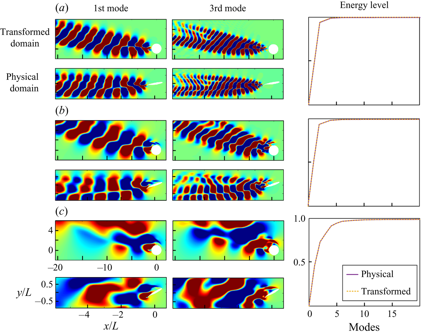
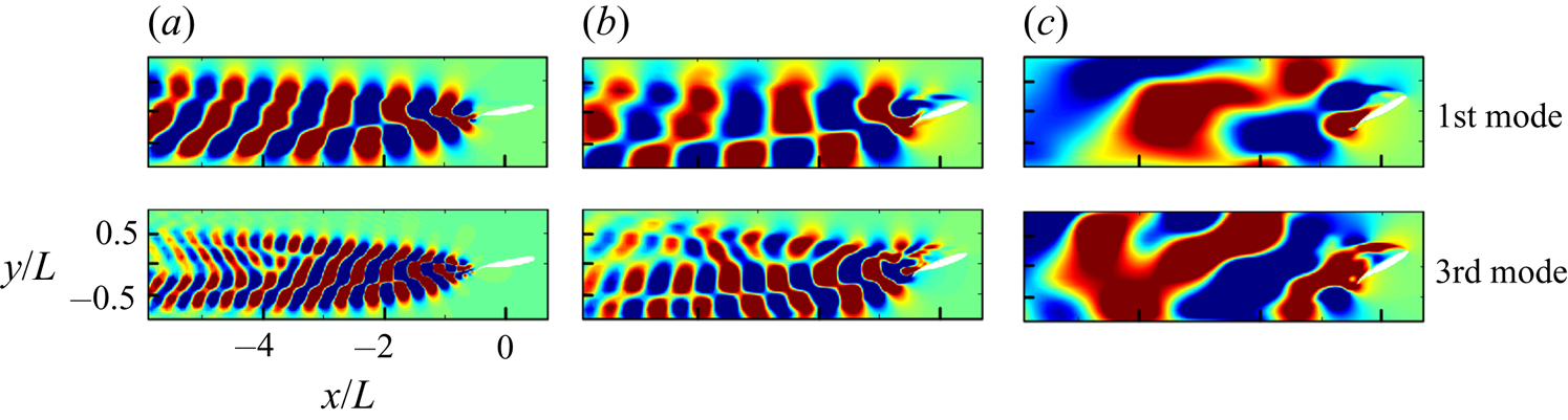
For simplicity, we only show the horizontal velocity component in figure 2. For all three cases with different AoA, the accumulative energy curves are identical across two different domains. As shown in figure 3, the modes are also found to be similar, proving the energy conservation nature of the conformal mapping process. In fact, the individual modes also contain the same energy content. An extra  $\boldsymbol {J}^{\textrm {T}} \boldsymbol {J}$ term is cancelled out with the domain expansion and contraction through the mapping process. This guarantees that the contribution of eigenvalues stays the same after the transformation. Therefore, the energy captured by each mode is also conserved. We will talk about how the mapping process affects the modal analysis performed with the vorticity next.
The first and third velocity POD modes and the normalized accumulative energy level in the transformed and physical domain of an airfoil with (a)  $10^{\circ }$, (b)
 $20^{\circ }$ and (c)
 $30^{\circ }$ angles of attack. For simplicity, the duplicate axis indices are not present.

The velocity POD modes of an airfoil with (a)  $10^{\circ }$, (b)
 $20^{\circ }$ and (c)
 $30^{\circ }$ angle of attack acquired in the transformed domain mapped to the physical domain. These modes are identical to the modes acquired in the physical domain in figure 2.

(ii) Vorticity: we start by inspecting the inner product:
 \begin{equation} R(\omega, \omega) = \langle \omega, \omega \rangle = \int_{\varOmega_z} \omega^*(z) \omega(z) \,\textrm{d}z = \int_{\varOmega_\zeta} \omega^*(\zeta) \omega(\zeta) |J|\,\textrm{d} \zeta. \end{equation}
Since the vorticity remains the same at corresponding locations through the mapping process, the same procedure brings forward an extra Jacobian term in the correlation factor. To recover the enstrophy in the physical domain, we can adopt a new definition of the geometrically weighted inner product:
 \begin{align} R_{GW}(v_1, v_2) & = \langle \boldsymbol{J}\boldsymbol{\cdot} v_1,\, \boldsymbol{J}\boldsymbol{\cdot} v_2 \rangle_{GW}\nonumber\\ & = \int_{\varOmega_{GW}} (\boldsymbol{J}\boldsymbol{\cdot} v_1(z))^* (\boldsymbol{J}\boldsymbol{\cdot} v_2(z))\, \textrm{d}z = \int_{\varOmega_{GW}} v_1^*(z)v_2(z)\, |J|\,\textrm{d}z. \end{align}
We will check if this modified product satisfies the principle definition of the inner product next. A vector space V with underlying field  $\mathbb {R}$ or
 $\mathbb {C}$ is known as an inner product when operation
 $\langle \,,\rangle$ satisfies the following conditions.
(a) Symmetry: for all vectors
$v_1$ and $v_2$, $\langle v_1, v_2\rangle = \overline {\langle v_2, v_1\rangle }$.(b) Linearity: for any scalar
$a$ and all vectors $v_1$, $v_2$ and $v_3$, $\langle av_1, v_2\rangle = \bar {a} \langle v_1, v_2\rangle$ and $\langle v_1, v_2+v_3 \rangle = \langle v_1, v_2 \rangle + \langle v_1, v_3 \rangle$.(c) Positive-definiteness: for any vector
$v$, $\langle v, v \rangle \geq 0$ and that $\langle v,v \rangle =0$ implies that $v=0$.


Now let us inspect if the product  $R_{GW}(v_1,v_2)$ satisfies these properties.
(a) Symmetry:
(2.35)\begin{equation} R_{GW}(v_1, v_2) = \langle \boldsymbol{J}\boldsymbol{\cdot} v_1,\, \boldsymbol{J}\boldsymbol{\cdot} v_2 \rangle_{GW} \nonumber\\ = \int_{\varOmega_{GW}} v_1^*(z)v_2(z)\, |J|\,\textrm{d}z = \overline{ \langle \boldsymbol{J}\boldsymbol{\cdot} v_2,\, \boldsymbol{J}\boldsymbol{\cdot} v_1 \rangle}_{GW}. \end{equation}(b) Linearity:
(2.36)\begin{align} R_{GW}(av_1, v_2) & = \langle \boldsymbol{J}\boldsymbol{\cdot} av_1,\, \boldsymbol{J}\boldsymbol{\cdot} v_2 \rangle_{GW} = \int_{\varOmega_{GW}} (a v_1(z))^*\,v_2(z)\, |J|\,\textrm{d}z\nonumber\\ & = \bar{a} \int_{\varOmega_{GW}} v_1^*(z)\,v_2(z)\, |J|\,\textrm{d}z = \bar{a}\langle \boldsymbol{J}\boldsymbol{\cdot} v_1,\, \boldsymbol{J}\boldsymbol{\cdot} v_2 \rangle_{GW}, \end{align}(2.37)\begin{align} R_{GW}(v_1, v_2+v_3) & = \langle \boldsymbol{J}\boldsymbol{\cdot} v_1,\, \boldsymbol{J}\boldsymbol{\cdot} (v_2+v_3) \rangle_{GW} = \int_{\varOmega_{GW}} v_1^*(z)(v_2+v_3)(z)\, |J|\,\textrm{d}z\nonumber\\ & = \int_{\varOmega_{GW}} v_1^*(z)v_2(z)\, |J| \,\textrm{d}z + \int_{\varOmega_{GW}} v_1^*(z)v_3(z)\, |J|\,\textrm{d}z\nonumber\\ & = \langle \boldsymbol{J}\boldsymbol{\cdot} v_1,\, \boldsymbol{J}\boldsymbol{\cdot} v_2 \rangle_{GW} + \langle \boldsymbol{J}\boldsymbol{\cdot} v_1,\, \boldsymbol{J}\boldsymbol{\cdot} v_3 \rangle_{GW}. \end{align}(c) Positive-definiteness:
(2.38)\begin{equation} R_{GW}(v, v) = \langle \boldsymbol{J}\boldsymbol{\cdot} v, \boldsymbol{J}\boldsymbol{\cdot} v \rangle_{GW} = \int_{\varOmega_{GW}} v^*(z) v(z) |J|\,\textrm{d}z \geq 0. \end{equation}


We see that the new definition satisfies all three criteria and, thus, represents a proper energy form that combines the flow energy and the structure motion with a proper weighting function. The key to this is that a conformal mapping always provides a positive Jacobian determinant. There is no fold-over in the mapping process, and the angle and topology are preserved. The geometric weighting is hence not arbitrary but coming from a unique transformation. For the scenarios in which weighting is not desirable, such as when the far-field flow feature is of primary interest, with a simple modification of the inner product, the effect can be removed from the modes.
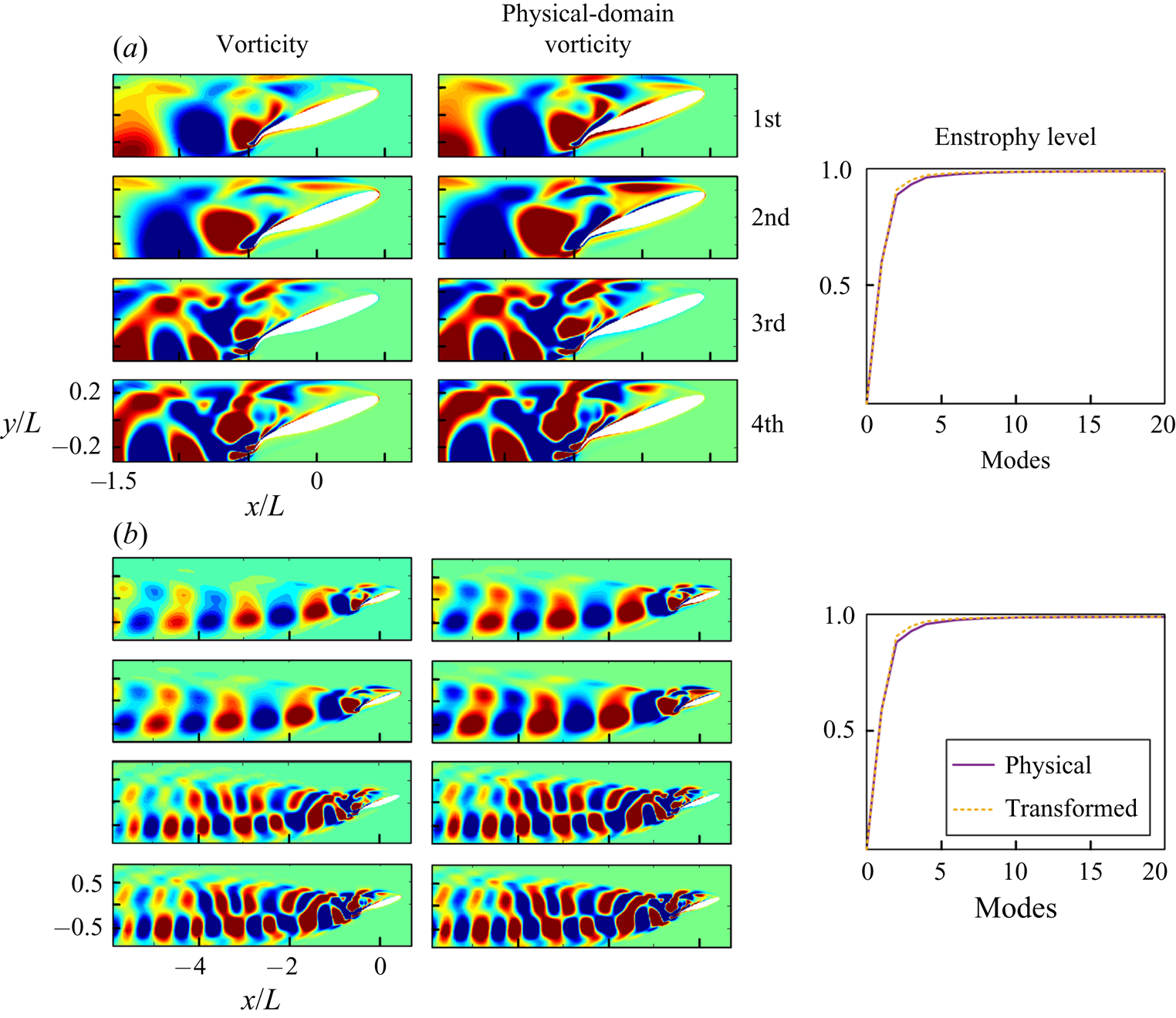
In figure 4 we provide examples with static geometry to illustrate this unique property of the mapping. We perform POD analysis of an airfoil with a  $20^{\circ }$ angle of attack in different settings: with and without the Jacobian modification. The modes acquired with the modified inner product
 $R_{GW}$ are denoted as the ‘physical-domain’ modes as the weighting counterbalance the mapping effect. When POD is performed in the near-body region, the modes and the accumulative enstrophy curves with or without the Jacobian modification are mostly the same. However, in the full-field modal analysis, the mode shapes show some differences in the wake, which result from the grid area expansion in the downstream location. Interestingly, the accumulative enstrophy curves are nearly identical in near-body and full-field cases, indicating that most of the enstrophy aggregates in the near-body region in this case.
The vorticity POD modes and accumulative normalized enstrophy level of an airfoil with  $AoA=20^{\circ }$ within (a) the near-body field and (b) an extended region, including further downstream.

Applying weights to data in order to emphasize the important aspect of a system can be seen in several previous works. For example, the weighted POD (Christensen, Brøns & Sørensen Reference Christensen, Brøns and Sørensen1999) and sequential POD (Jørgensen et al. Reference Jørgensen, Sørensen and Brøns2003) assign weights to the snapshots to detect the low energetic yet dynamically important modes. The phase-invariant POD (Fogleman et al. Reference Fogleman, Lumley, Rempfer and Haworth2004) stretches the velocity field in one direction to bring the POD modes to the same configuration, which a similar strategy is also used for a backward-facing ramp (Taylor & Glauser Reference Taylor and Glauser2004). The proposed method here offers a systematic weighting function through the unique benefit of the conformal mapping, and if necessary, the users can recover the physical-domain enstrophy with the modified inner product.
On the other hand, the DMD modes represent the dynamics with specific characteristic frequencies. In the proposed method,  $\boldsymbol {A}$ or
 $\boldsymbol {B}$ matrices identify how the system evolves over time in the transformed space. The conformal mapping provides a time-invariant frame for the spatial modes to embed on in the transformed space. The deforming or moving body in the fluid can be seen as a sharp boundary sweeping through the fluid domain, and approximating such motion in the Eulerian domain requires an infinite number of linear modes. The GW-MD instead integrates the nonlinear effect into a Laplacian-conserved mapping between domains to avoid the problem.
The method described above shows several significant benefits. First, based on the uniformization theorem, there is a conformal connection between any simply connected Riemann surface with one of three canonical shapes of the unit disk, the complex plane or the Riemann sphere. Hence, there is no restriction to the geometries other than being smooth. Secondly, it does not demand an additional definition of energy or prior knowledge of the system. Also, all the available extended versions of the modal analysis techniques, such as the aforementioned online DMD or multiresolution DMD (mrDMD), can be readily deployed. The proposed method is also applicable to both experimental and computational data provided the geometry contour is available. In those cases, the conformal mapping procedure can be applied in post-processing modal analysis. A similar idea of post-applying modal analysis techniques is suggested by Troshin et al. (Reference Troshin, Seifert, Sidilkover and Tadmor2016) and tested on a set of heaving airfoil results.
Reduced-order modelling can also benefit from the modal analysis. One of the advantages of POD modes is that they form optimal orthogonal bases to reduce the governing equations into sets of ordinary differential equations with techniques such as the Galerkin projection. Through this procedure, the nonlinear system can be approximated with a reduce-order model (ROM) that could represent the original system with adequate accuracy. Nevertheless, for systems with deforming or moving boundaries, the lack of a proper technique to obtain POD modes restricts the ROM development. Anttonen, King & Beran (Reference Anttonen, King and Beran2003) looked at a case of potential flow over an oscillating panel by performing POD on a deforming grid, which is generated by holding the same grid number in the vertical direction. Freno & Cizmas (Reference Freno and Cizmas2014) further explored the problem using a dynamic average base flow and basis functions and showed that this method can recover the flow features better than standard snapshot POD modes. Liberge & Hamdouni (Reference Liberge and Hamdouni2010) proposed the multiphase POD method to extend the Navier–Stokes equations to the solid domain by using a penalization method and indicated its effectiveness in reconstructing flow over an oscillatory cylinder. The proposed method is in line with the principle of these previous techniques, with the main difference that here the solid motion is systematically lifted and embedded into the governing flow equations in a fixed domain such that it preserves important flow properties. It can also equivalently be formulated as a partial differential equation constraint mapping method in the celebrated topological manifold submersion and immersion techniques in differential topology (Lang Reference Lang2012). If the deformation of the surface is accessible, one can form ROMs of the flow dynamics using the GW-POD modes. One shortcoming of the proposed method is the lack of information about the solid internal dynamic in the process of developing the ROM in the reference domain. A potential remedy is to extend the mapping with a proper complementary energy function for the solid deformation to obtain the hybrid flow-solid POD modes concurrently (Goza & Colonius Reference Goza and Colonius2018). An alternative technique is to identify the POD modes of the deformable geometries in their Lagrangian domains and employ their reconstructed surface motion to form a ROM of the flow dynamics. This method is particularly suitable for FSI problems in which the time scales of the solid domain are narrow-band imposed by its natural frequencies while the flow includes a broad range of dynamically important frequencies.
A limitation of the proposed method is that it is restricted to two-dimensional systems since conformal mapping primarily exists for two-dimensional space. For general two dimensional embedded surfaces in three-dimensional (3-D) space, techniques such as Riemann mapping, cone singularities, Cauchy–Riemann equation, Ricci flow or Dirac equation can be employed to form the conformal mapping between two arbitrary surfaces. The extension of a full conformal mapping to higher dimensions is only feasible through Mobius transformation according to Liouville's theorem (Flanders Reference Flanders1966). However, many quasi-conformal techniques are still available to form a flexible 3-D mapping between volumes with minimal distortion from fully conformal mapping (Hurdal et al. Reference Hurdal, Bowers, Stephenson, De Witt, Rehm, Schaper and Rottenberg1999; Gu et al. Reference Gu, Wang, Chan, Thompson and Yau2004; Li & Hartley Reference Li and Hartley2007; Zeng & Gu Reference Zeng and Gu2011). Also, for systems involving multiple deforming or moving volumetric bodies, methods such as the large deformation diffeomorphic metric mapping (Beg et al. Reference Beg, Miller, Trouvé and Younes2005; Cao et al. Reference Cao, Miller, Winslow and Younes2005; Vercauteren et al. Reference Vercauteren, Pennec, Perchant and Ayache2007) can be employed to optimally equip the domain with a differential background transport equation and enable the use of modal analysis to multibody systems.
3. Illustrative examples
Three examples of an undulating fish, a shape-changing ellipsoid and an airfoil with an active deflecting flap are selected to showcase the capabilities of the geometrically weighted modal analysis technique in dissecting the flow and forming a reduced-order representation of the flow.
3.1. Undulating fish
A fish model with undulatory motion is selected here to demonstrate the effectiveness of applying the geometrically weighted modal analysis to a deforming geometry. Using undulation as their primary propulsion method, fishes can swim with unparalleled maneuverability and efficiency compared with underwater vehicles. The famous experiment of the carcass of a rainbow trout passively undulating upstream (Beal et al. Reference Beal, Hover, Triantafyllou, Liao and Lauder2006) shows how important the interaction between the body deformation and surrounding flow field is. To learn from the aquatic animals, observations (Gray Reference Gray1933; Blake Reference Blake1983; Sfakiotakis, Lane & Davies Reference Sfakiotakis, Lane and Davies1999; Videler Reference Videler2012) and metabolic rate measurements (Webb Reference Webb1971; Clarke & Johnston Reference Clarke and Johnston1999; Gillooly et al. Reference Gillooly, Brown, West, Savage and Charnov2001) are made, and different models have been proposed to explain the mechanics of fish swimming (Gero et al. Reference Gero1952; Lighthill Reference Lighthill1960; Wu Reference Wu1971). These observations and models have been used to design and build several fish robots and undulatory propellers (Triantafyllou & Triantafyllou Reference Triantafyllou and Triantafyllou1995; Yu et al. Reference Yu, Tan, Wang and Chen2004; Liu & Hu Reference Liu and Hu2010; Marchese, Onal & Rus Reference Marchese, Onal and Rus2014). Computational fluid dynamics methods have been utilized to study fish locomotion. Techniques such as the vortex particle method (Ojima & Kamemoto Reference Ojima and Kamemoto2005; Eldredge & Pisani Reference Eldredge and Pisani2008; Shoele & Zhu Reference Shoele and Zhu2015), Euler–Lagrangian method (Kern & Koumoutsakos Reference Kern and Koumoutsakos2006) and immersed boundary method (Bozkurttas et al. Reference Bozkurttas, Dong, Mittal, Madden and Lauder2006; Borazjani & Sotiropoulos Reference Borazjani and Sotiropoulos2008; Tytell et al. Reference Tytell, Hsu, Williams, Cohen and Fauci2010; Maertens, Gao & Triantafyllou Reference Maertens, Gao and Triantafyllou2017) allow more delicate studies of fish swimming due to their capabilities to obtain high resolution full-field flow data. However, the methods either employ a deforming grid or require grid interpolation at the body contour, and this prevents the classical data-driven modal analysis tools from being employed to investigate the full flow field. Geometrically weighted modal decomposition solves this problem by transforming the undulating fish into a fixed cylinder with a time-invariant grid attached.
The fish model examined here is chosen to be a modified NACA0012 airfoil. The camber of the NACA0012 airfoil undergoes a lateral oscillation in the form of a streamwise downward travelling wave, described by
 \begin{equation} y_0=A_m(x)\cos\left[2{\rm \pi}(x+c\,t)\right], \quad 0\leq x\leq 1, \end{equation}
where  $A_m$ is the amplitude normalized with the fish length and
 $c$ is the phase speed of the travelling wave relative to the free stream velocity. From the experimental data of a steadily swimming saithe (Videler & Hess Reference Videler and Hess1984), the backbone undulation motion of a fish can be approximated by a quadratic polynomial
 \begin{equation} A_m(x)=C_0+C_1x+C_2x^2, \end{equation}
where the coefficients  $C_0$,
 $C_1$ and
 $C_2$ are obtained from the recorded kinematic data, which gives
 $A_m(0)=0.02$,
 $A_m(0.2)=0.01$ and
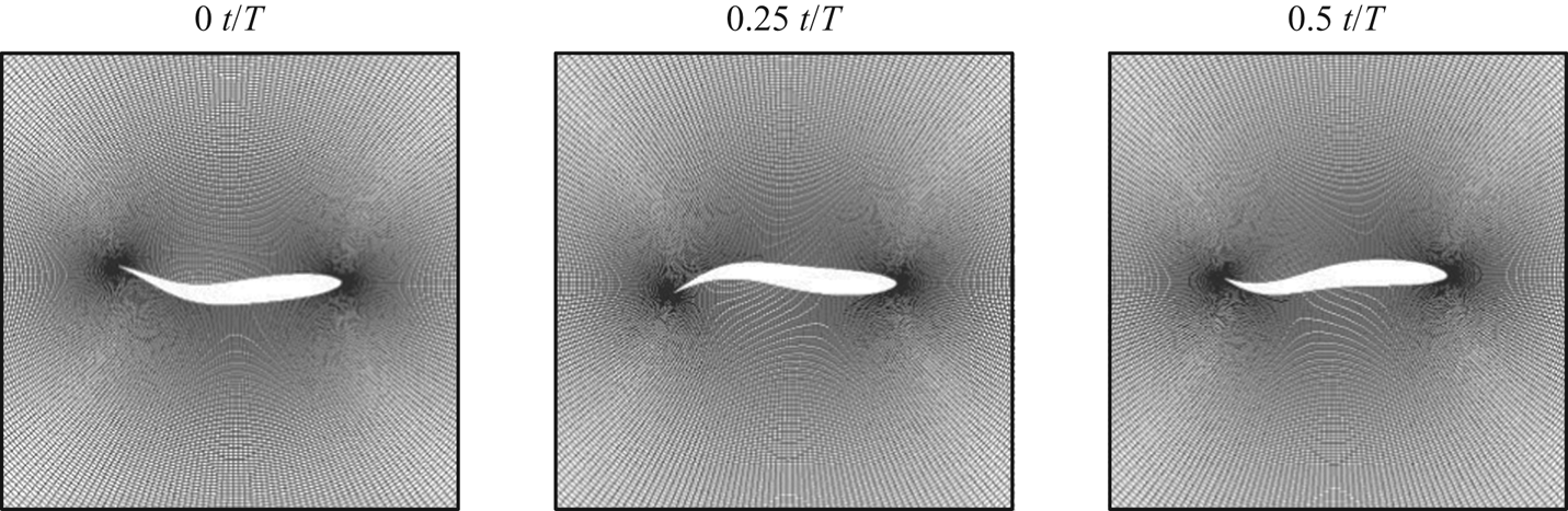
 $A_m(1)=0.1$. This profile is also used in many other types of research like Dong & Lu (Reference Dong and Lu2007) and Borazjani & Sotiropoulos (Reference Borazjani and Sotiropoulos2008). The undulation motion is imposed as a pure lateral motion (Wassersug & von Sechendorf Hoff Reference Wassersug and von Sechendorf Hoff1985; Liu et al. Reference Liu, Wassersug and Kawachi1996). Three snapshots of the fish geometry are shown in figure 5. In this section we are going to show two cases with the same phase speed
 $c=4$ but different Reynolds number
 $Re=U_\infty L/\nu =1000, 4000$. We will focus on the near-body flow field to examine the performance of the GW-MD technique in capturing the near-body flow features.
Snapshots of the deforming grid around the undulating fish model. Here  $T$ represents the normalized period of the deformation.

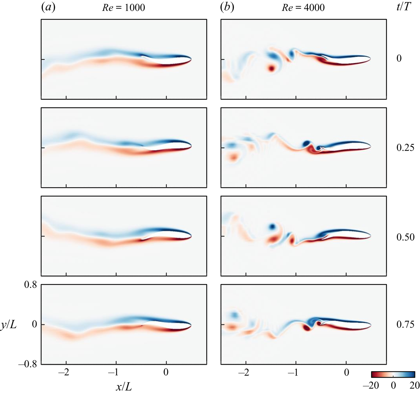
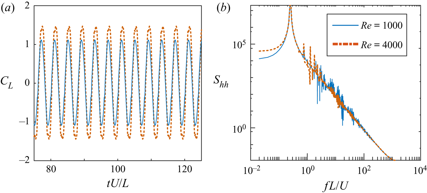
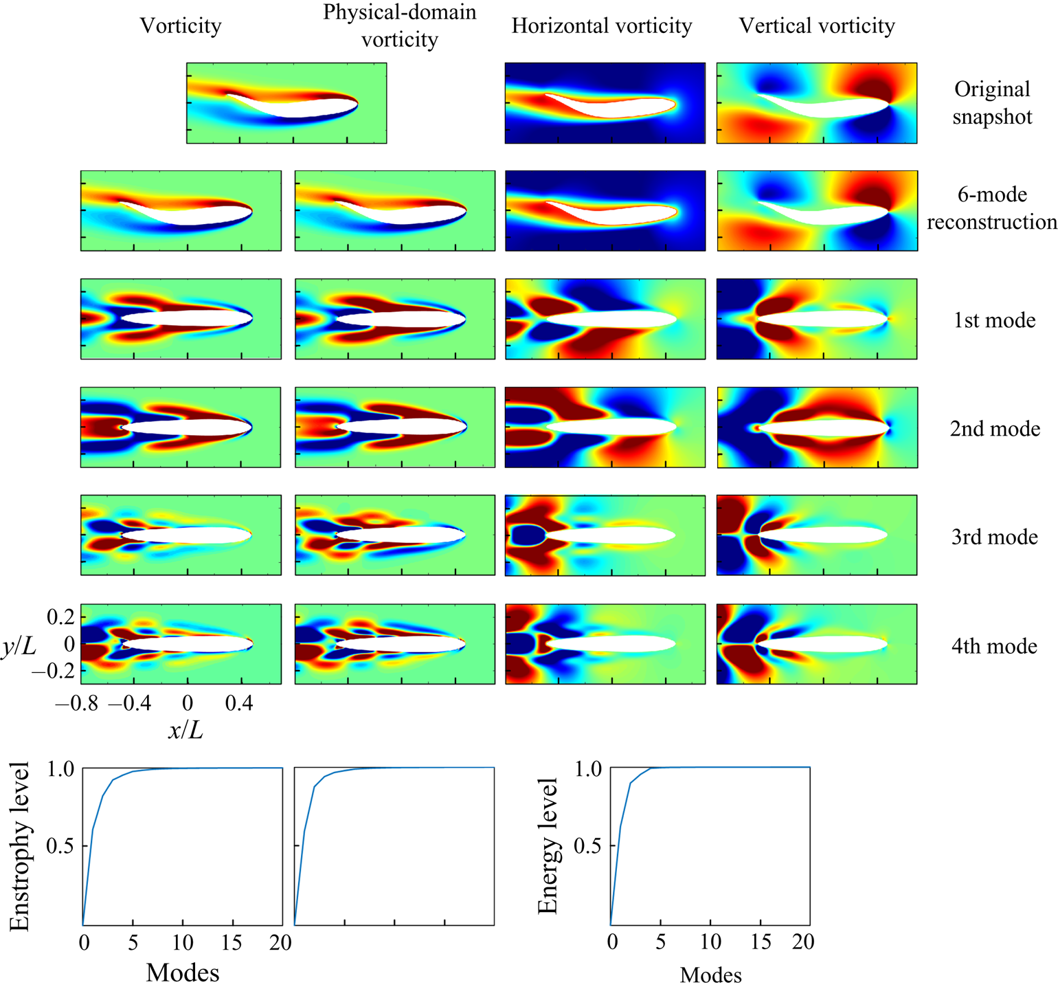
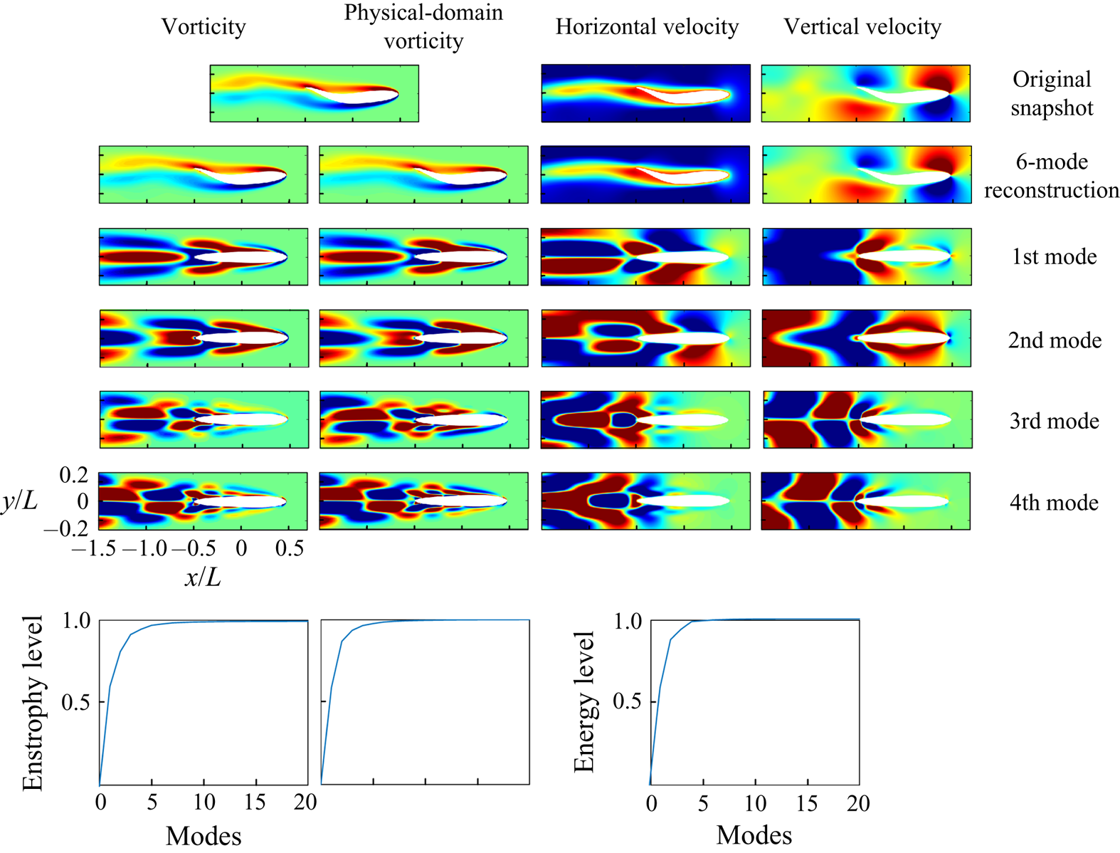
The snapshots of the vorticity field behind the fish are shown in figure 6. From the time history and power spectrum of the lift coefficient plotted in figure 7, it is found that for both Reynolds numbers, the fish experiences periodic forcing at frequency  $St=0.25$, defined based on the free stream velocity and chord length. However, in the higher Reynolds number the vortices break down closer to the body and form multiple clusters. For all the following examples, the number of snapshots used in the modal analysis process covers at least 30 structural motion cycles with at least 10 snapshots per cycle. Figure 8 shows the GW-POD modes for the
 $Re=1000$ case. The first column is obtained by directly applying the snapshot POD procedure to the vorticity in the transformed domain. For the second column, we premultiplied the vorticity with
 $\sqrt {|J|}$ to mitigate the transformation effect and denoted this as the physical-domain vorticity. The third and fourth columns show the horizontal and vertical velocities of GW-POD modes acquired in the transformed domain. As explained in the previous section, the Jacobian, in this case, has a greater determinant value at the trailing edge and the parts of the body with a large curvature. To help understand where the energy aggravates around the deforming body, we place the acquired modes on the grid constructed around the mean geometry. Note that the velocity modes are residing on the time-invariant grid in the transformed space, and mapping them to the mean grid is a visualization procedure.
Snapshots of the undulating fish cases with the phase speed  $c=4$ and different Reynolds numbers
 $Re=1000, 4000$. Here
 $T$ is the period of the motion. The colours represents the vorticity range.

(a) Time history and (b) power spectrum of the lift coefficient of the undulating fish model.

Geometrically weighted proper orthogonal decomposition modes, reconstruction of the snapshot and accumulated energy (enstrophy) level of the near-body flow field with the phase speed  $c=1$ and
 $Re=1000$. To avoid cluttering the duplicate figure axis labels are not shown.

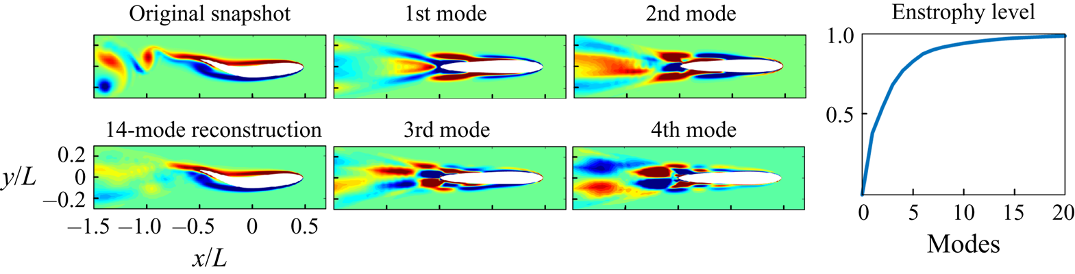
It is found that less than six modes are required to capture over  $95\,\%$ of the energy or enstrophy, regardless of which variable is selected to perform the GW-POD. The difference between using the vorticity or physical-domain vorticity is that the physical-domain modes have more emphasis on the leading edge region. Figure 9 shows the same modes with the inclusion of a wider downstream region. The reconstruction is still very efficient as only six leading modes recover
 $95\,\%$ of the energy content. We can observe that the vorticity modes capture more details in the wake than the physical-domain vorticity modes. Both the vorticity and velocity modes display that most of the energy is accumulated around the mid-section and the trailing edge, where the primary vortex shedding happens. We can also observe that there are three sections with alternative vorticity along the body due to the sinusoidal wave shape. Since all three analyses using different variables have similar results, we will only report the modal analysis using the unmodified vorticity variable in the rest of the paper.
Geometrically weighted proper orthogonal decomposition modes, reconstruction of the snapshot and accumulated energy (enstrophy) level of the further downstream region flow field with the phase speed  $c=1$ and
 $Re=1000$.

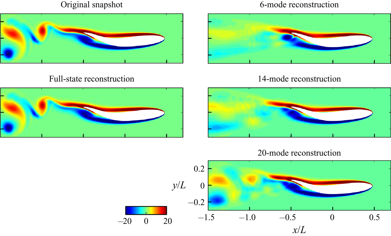
Now we look at the higher Reynolds number case. This case also includes a periodic flow, but instead of the more continuous wake observed in the  $Re=1000$ case, the wake consists of alternative vortices. The GW-POD modes are shown in figure 10 and it is noticed that the higher Reynolds number affects the dominant modes of the flow in two significant ways: the lack of coherent structures at further downstream locations and the need for more modes to reconstruct the flow field. The vortices shed from the trailing edge are propagating downstream as a vortex street, and more harmonic mode shapes are required to capture these coherent structures correctly. As a result, with only six modes, the reconstruction can hardly recover any wake distribution. Even with 14 modes, which contain just over
 $95\,\%$ of the enstrophy disturbance, the downstream region is still not represented well (figure 11). However, vorticity distribution in the near-body region does not change much with the inclusion of higher modes. One should anticipate that since the force experienced by the body is mostly affected by the near-body vortex distribution, the hydrodynamic force acting on the body can be recovered with fewer modes than otherwise needed to reconstruct the whole flow field.
Geometrically weighted proper orthogonal decomposition modes, reconstruction of the snapshot and accumulated energy (enstrophy) level of the vorticity field in the further downstream region with the phase speed  $c=1$ and
 $Re=4000$.

Reconstruction of the vorticity field with different numbers of modes for the case with phase speed  $c=1$ and larger Reynolds number
 $Re=4000$.

The undulating fish model shows how conformal mapping enables the modal analysis to be employed to study the flow field around a deforming body. The modes extracted with different variables have different indications of the dynamics but have similar reconstruction performance. Through two illustrative cases, we observe that the GW-POD modes can identify where the energy aggregates and reveal that the near-body vorticity distributions are similar in the dominant modes. Hence, we can explain why the force profiles are alike despite the very different wake. In the next section we will show how the geometrically weighted dynamic mode decomposition (GW-DMD) modes can be used to isolate system dynamics with characteristic frequencies.
3.2. Shape-changing ellipsoid
Deforming bodies in the flow stream have many engineering and biological applications such as icing plane wings (Bragg, Gregorek & Lee Reference Bragg, Gregorek and Lee1986) or dissolving icebergs (Taylor Reference Taylor1953; Eames Reference Eames2008; Weymouth & Triantafyllou Reference Weymouth and Triantafyllou2012), insect flight and ocean animals swimming by sudden shape change (Childress, Vandenberghe & Zhang Reference Childress, Vandenberghe and Zhang2006; Steele, Weymouth & Triantafyllou Reference Steele, Weymouth and Triantafyllou2017). In this section we consider a canonical case of a deforming ellipsoid. As said in the previous section, we will use the vorticity in the transformed domain as the analysis object as it better captures the near-body flow field.
The geometry inspected here follows the work of Spagnolie & Shelley (Reference Spagnolie and Shelley2009). The semi-major axis  $a(t)$ and semi-minor axis
 $b(t)$ of the body are changing with time, while the area of the ellipse
 ${\rm \pi} a(t)b(t)$ is kept constant. The periodic deformation of the body is defined by
 \begin{equation} a(t)=\frac{1}{4}\left[5+\sin(2{\rm \pi} t)\right]\quad \text{and} \quad b(t)=\frac{1}{a(t)}. \end{equation}
Several snapshots of the ellipsoid deformation and the corresponding body-fitted grid are shown in figure 12. The ambient flow velocity  $U_\infty$ is used as the velocity scale, and the characteristic length is related to the area and defined as
 $L=\sqrt {a(t)b(t)}$. Here the Reynolds number is fixed at
 $Re=U_\infty L/\nu =1000$.
An ellipsoid expanding and contracting in the  $X$-direction. Here
 $T$ represents the normalized period of the deformation.

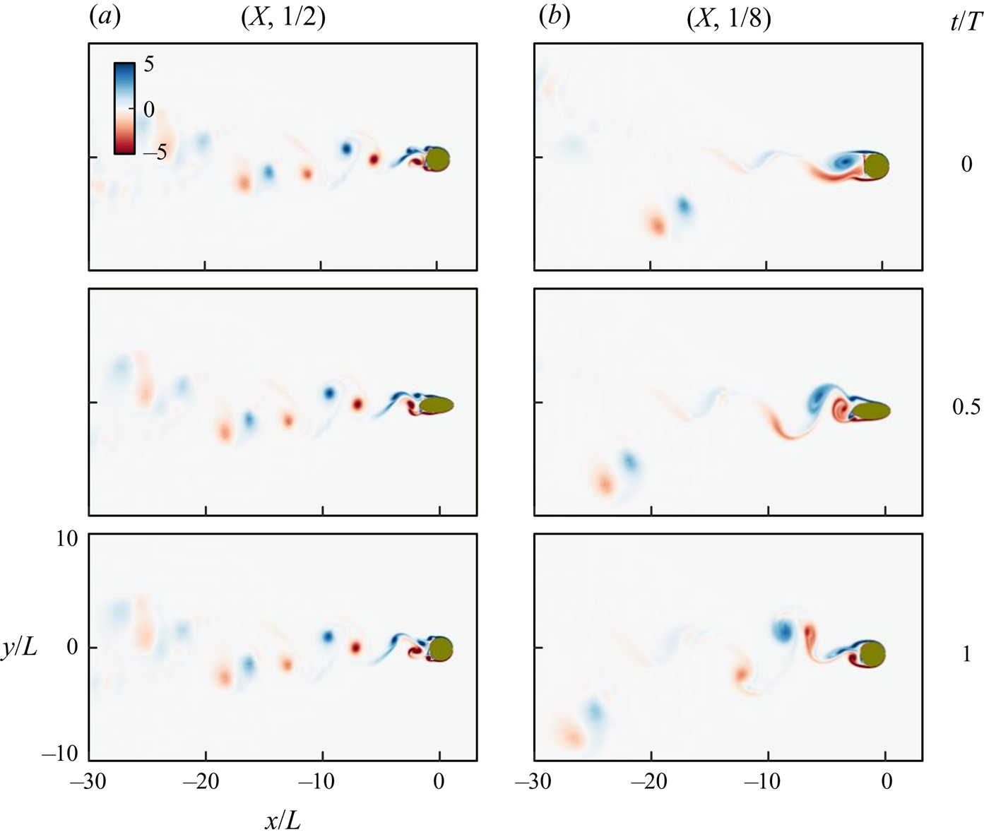
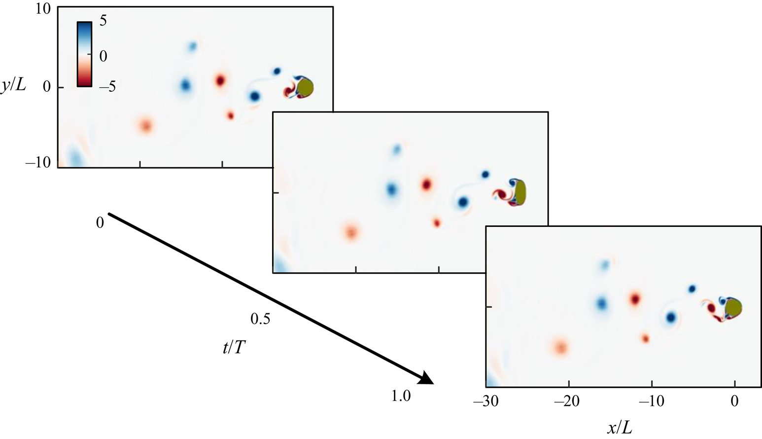
In this section we focus on the effect of different deforming frequencies and the principal stretching direction on the flow around the body. We will use the pair (elongation direction, Strouhal number  $St=f\,L/U_\infty$) to represent different cases. Figure 13 displays snapshots of the vorticity field of two cases,
 $(X, 1/2)$ and
 $(X, 1/8)$. While it is very challenging to understand the impact of the deformation on the flow from the snapshots alone, GW-DMD can be applied to the transformed cylindrical domain to investigate the modal frequency content of the flow field. Here, for brevity, only the real part of each GW-DMD mode is shown as similar observations can be made for the imaginary part.
Snapshots of the vorticity field of the deforming ellipsoid for (a)  $(X, 1/2)$ and (b)
 $(X, 1/8)$ over one structural motion period.

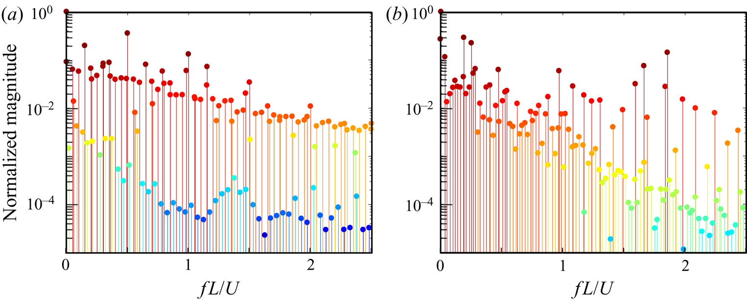
The frequency-magnitude plots of the principal eigenvalue of GW-DMD modes for both cases are shown in figure 14. It is observed that for the  $(X, 1/2)$ case, the harmonics of
 $St=0.5$ (the frequency of the geometry deformation) have large peaks in magnitude; whereas such peaks are not present in the
 $(X, 1/8)$ case and the first three most significant peaks are at
 $St=0.1916, 0.0045, 0$. The comparison of the spatial GW-DMD modes in the transformed domain, as shown in figure 15, reveals the difference between the two cases. The modes of the
 $(X, 1/2)$ case have a periodic wake with distinct alternative vortices shedding within a narrow region right behind the trailing end. The dominant modes have the inherent frequencies of the harmonics of the geometry change. On the other hand, the
 $(X, 1/8)$ case does not possess coherent spatial modes and instead the vortices distribute throughout the whole domain, forming a broad wake behind the body. These modes have frequencies that are not directly connected to body motion.
Frequency-magnitude plot of the GW-DMD modes of the case (a)  $(X, 1/2)$, (b)
 $(X, 1/8)$.

The first three GW-DMD vorticity mode pairs of the case (a)  $(X, 1/2)$ and (b)
 $(X, 1/8)$ are shown from top to bottom in order.

We can now see how body motion impacts the flow field from the snapshots shown in figure 13. In the  $(X, 1/2)$ case the ellipsoid expands and contracts at a relatively fast rate compared with the vortex shedding time scale, and each time it elongates the vortices convect only a small distance downstream. However, before the vortices can completely separate away from the body, the ellipsoid body contracts and causes a reverse flow. This, in return, stops the shedding and forms a chain of smaller vortices near the surface. The pressure gradient formed by the vortex chain eventually affects the breakup of the shear layer and results in a wake that resembles the von-Karman vortex street. Hence, the vortex shedding frequency is controlled by the frequency of the shape changing.
Conversely, the  $(X, 1/8)$ case shows a weak correlation between the vortex shedding and deformation. The reason is that the deformation occurs much slower compared with the previous case where strong reverse flow and suppression of the boundary layer separation are present. Here the vortices are formed based on the instantaneous geometry, and as a result, the chaotic behaviours with unsteady vortex shedding frequencies emerge.
Now we turn our focus to how the elongation direction affects the flow field. In figure 16 snapshots of the case  $(Y, 1/2)$ are shown wherein the vortices appear in a broader area in the wake and do not follow any pattern. This observation can be explained by the presence of a powerful reverse flow from the large elongation in the cross-flow direction. Here the reverse flow with a large pressure gradient is so strong that the vortex shedding becomes unstable, quite different from the
 $(X, 1/2)$ case where the reverse flow is weak and the separated vortices are close to the body. To further investigate this observation, we compare the GW-POD representations of both
 $(X, 1/2)$ and
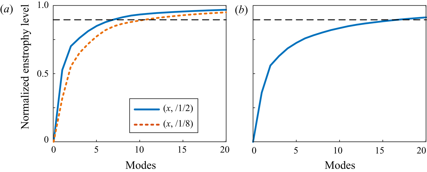
 $(Y, 1/2)$ cases. In figure 17 we see a distinctive difference in the accumulative normalized energy level. In the
 $(X, 1/2)$ case more than
 $90\,\%$ of its energy is in the first seven modes while the
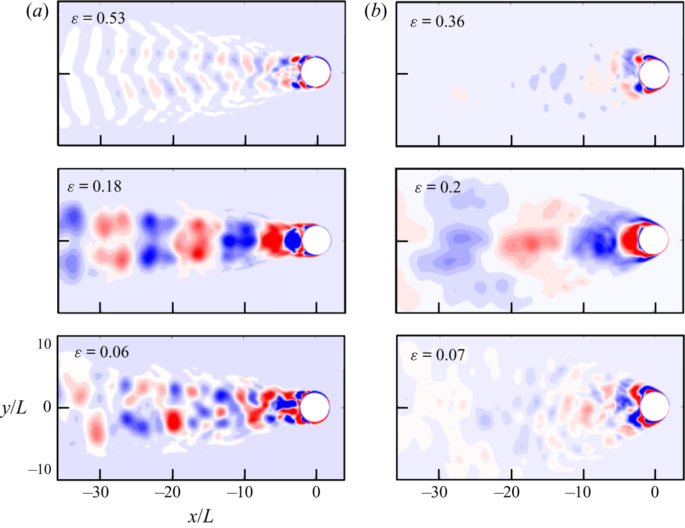
 $(Y, 1/2)$ case requires 18 modes to reach the same level. This comparison shows the lack of coherent structures in the
 $(Y, 1/2)$ case and can be further supported by the spatial modes shown in figure 18. Compared with the alternative vortex pairs found in the leading GW-POD modes of the
 $(X, 1/2)$ case, the most energetic modes of the
 $(Y, 1/2)$ case exhibit a broad wake. In this case, the energy aggregates closer to the body due to the sparse wake and the near-body reverse flow.
Snapshots of the vorticity field of deforming ellipsoid case  $(Y, 1/2)$ over one structural motion period.

Normalized accumulative energy level of GW-POD vorticity modes for cases (a)  $(X, 1/2)$ and
 $(X, 1/8)$, (b)
 $(Y, 1/2)$. The dashed line denotes the 90 % accumulated enstrophy level.

The first three most energetic GW-POD vorticity modes of the cases (a)  $(X, 1/2)$ and (b)
 $(Y, 1/2)$ shown from top to bottom. The normalized energy level
 $\epsilon =\lambda _i/\sum _{i} \lambda _i$ of each mode is overlaid.

For a periodic system, it can be useful to reconstruct the flow fields with truncated modes. This eliminates the less energetic modes often contaminated with noise and numerical errors and permits representing the system with less complexity. Figure 19 shows instantaneous snapshots for the  $(X, 1/2)$ and
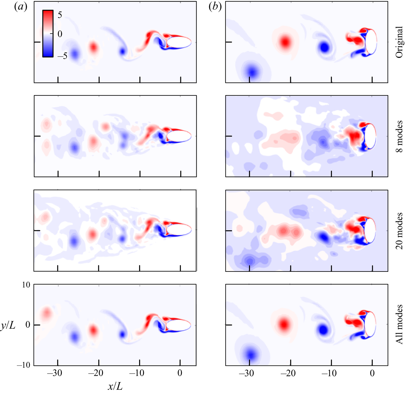
 $(Y, 1/2)$ cases and their reconstruction with a different number of GW-POD modes. It can be seen that with only eight modes, the reconstruction can capture most of the vorticity distribution in the
 $(X, 1/2)$ case, while in the
 $(Y, 1/2)$ case even with 20 modes, the reconstruction is not able to represent the flow field well. Furthermore, by using the geometrically weighted technique, the near-body dynamically critical flow features are given higher weights and the near-body flow field is captured with the first dominant modes while the higher modes essentially correct the vortices far from the ellipse.
Reconstruction of the vorticity field of cases (a)  $(X, 1/2)$ and (b)
 $(Y, 1/2)$ with different numbers of GW-POD modes. The top row shows the original snapshot.

In this section we used three cases of the shape-changing ellipsoid problem to demonstrate how the GW-MD can reveal the crucial dynamics of a system involving flow and deforming geometry. The characteristic frequencies acquired from GW-DMD successfully separate the effect of the deformation versus the spatial fluid modes. The results show that the computed GW-POD modes are a good candidate to form a reduced-order representation of the flow field.
3.3. Oscillating airfoil with an active deflecting flap
Oscillating airfoils appear in diverse systems, such as the flutter of the aircraft wings (Kehoe Reference Kehoe1995), animal locomotion (Guglielmini & Blondeaux Reference Guglielmini and Blondeaux2004) or renewable energy extraction devices (Zhu & Peng Reference Zhu and Peng2009). To achieve better control of the oscillation of the airfoil, NASA and Boeing collaborated to develop the EET high-lift airfoil (Morgan Reference Morgan2002). The airfoil is equipped with actuators that can extend and deform the airfoil contours. We adopt this system as an example and focus on applying the GW-MD technique to inspect how the active deformation of the flap affects the flow structure in the wake. This system involves the feedback from the fluid loading force to the solid motion and exhibits a wide range of motion.
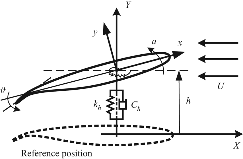
Figure 20 shows the physical model of an EET high-lift airfoil with the active trailing-edge flap. The physical parameters of the system include the geometric angle of attack  $\alpha$ of the airfoil relative to the horizontal direction, the heaving displacement
 $h$ and the angle of the flap relative to the mean chord of the foil
 $\theta$. The aeroelastic oscillating effect is modelled by a set of linear and torsional spring-damper systems with damping and stiffness coefficients of
 $c_{h/\alpha }$ and
 $k_{h/\alpha }$, respectively.
The physical model of an EET high-lift airfoil.

The comprehensive study of the dynamics of this system was discussed more in-depth in Wang & Shoele (Reference Wang and Shoele2018), and here the main focus instead is on the use of modal analysis to differentiate the flow structures between different cases.
The foil is fixed at an angle of attack  $\alpha$ and a sinusoidal oscillation is imposed on the flap to study how the flap motion influences the airfoil movement. The flap angle is
 $\theta =\theta _0+A\,\sin (\varOmega t)$, where
 $\theta _0$ and
 $A$ are the mean angle and amplitude, respectively, and
 $f=\varOmega /2{\rm \pi}$ is defined as the frequency of the oscillation. The Reynolds number (
 $Re=U_\infty L/v$) based on the chord length of the foil
 $L$ is chosen to be 1000. The flap length is
 $l=0.12L$. In the rest of this section we use the Strouhal number,
 $St=fL/U_\infty$, to differentiate different cases while keeping other parameters fixed at
 $\alpha =10^\circ$,
 $A=1.5^\circ$ and
 $\theta _0=23.5^\circ$.
Two cases with the flap frequency  $St=0.1$ and
 $0.9$, along with the control group with a stationary flap
 $St=0$, are selected for this discussion. Figure 21 plots the heaving displacement time history of the airfoil and its power spectrum. The frequencies of the power peaks are denoted on the plot. We also provide the phase portrait plot, which is the mapping between the heaving displacement
 $h$ and velocity
 $dh/dt$, coloured from white to black in the temporal order.
From left to right are time histories of heaving displacement, power spectrum and the phase portrait plot of cases  $St={0.0, 0.1, 0.9}$ respectively shown from the top to bottom row.

From the control group, we observe a steady periodic vibration of the airfoil with frequency  $St=0.96$, as proved by the single-cycle phase portrait and a single dominant peak in the power spectrum. The heaving motion at the natural frequency is caused by the interaction between the alternative vortex shedding and the linear spring-damper system. When the actuation is activated, both the
 $St=0.1$ and
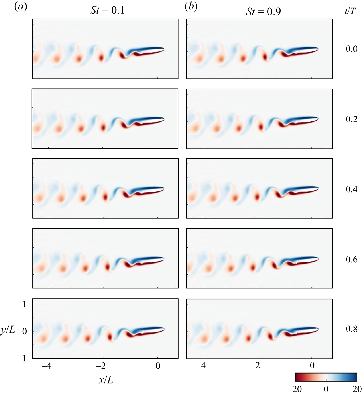
 $St=0.9$ cases exhibit a large heaving motion. The instantaneous snapshots within one actuation period for both cases are plotted in figure 22, which show a very similar wake profile and heaving amplitude between the two cases. It is possible to identify from the power spectrum and the torus-projected phase portrait that both cases are quasi-periodic systems with two distinct frequencies. However, the natural frequency
 $fL/U_\infty =0.96$ is only present in the
 $St=0.1$ case. Some questions arise from these observations: what role does the active flap play in creating these large-amplitude motions compared with the control case? What is the difference between the two actuated cases when their heaving time histories look similar? What flow features are connected to the dominant frequencies identified from the structural motion?
Instantaneous vorticity field of (a)  $St=0.1$ and (b)
 $St=0.9$. The time span between each figure is normalized with the structural deformation period.

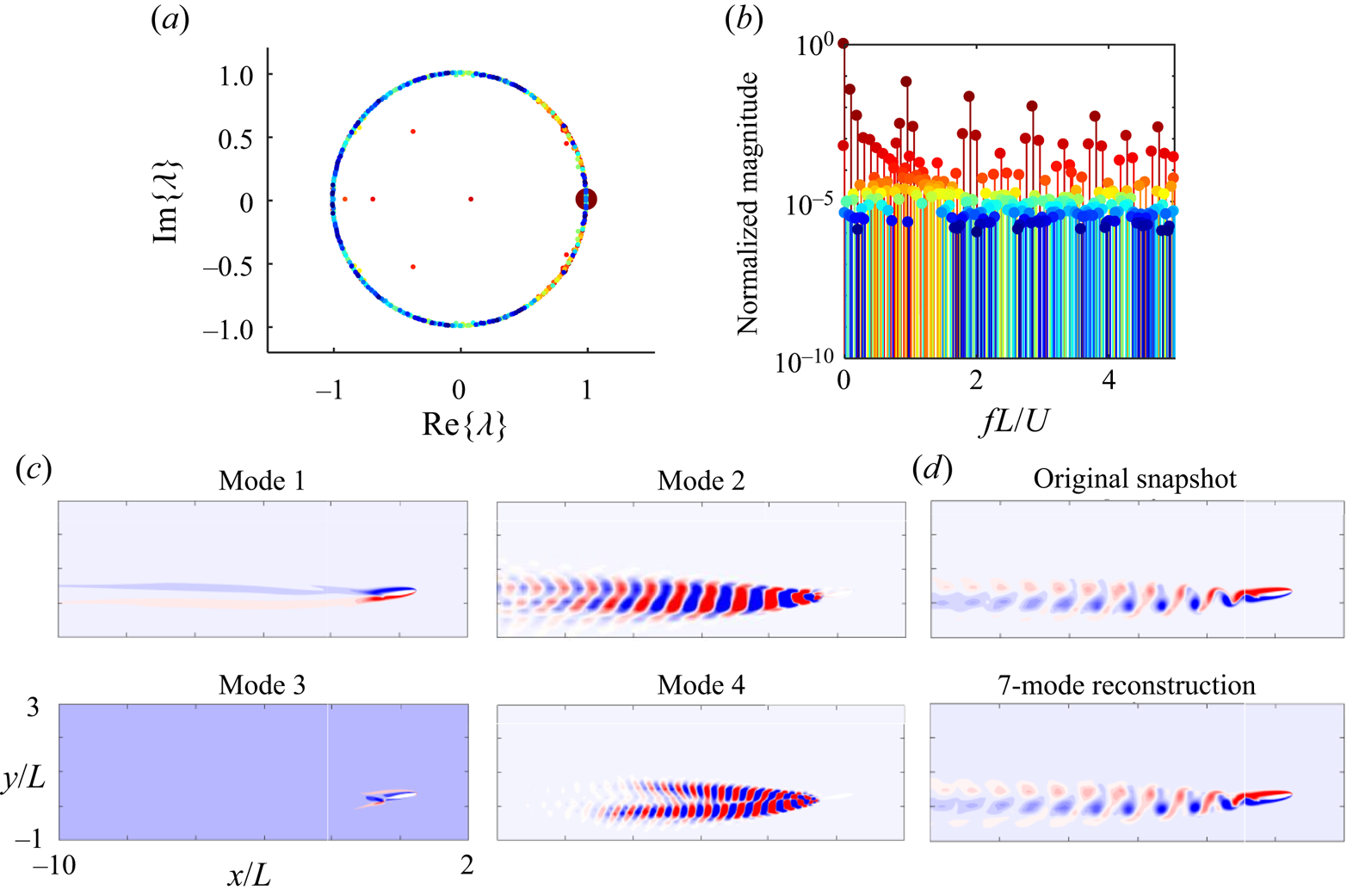
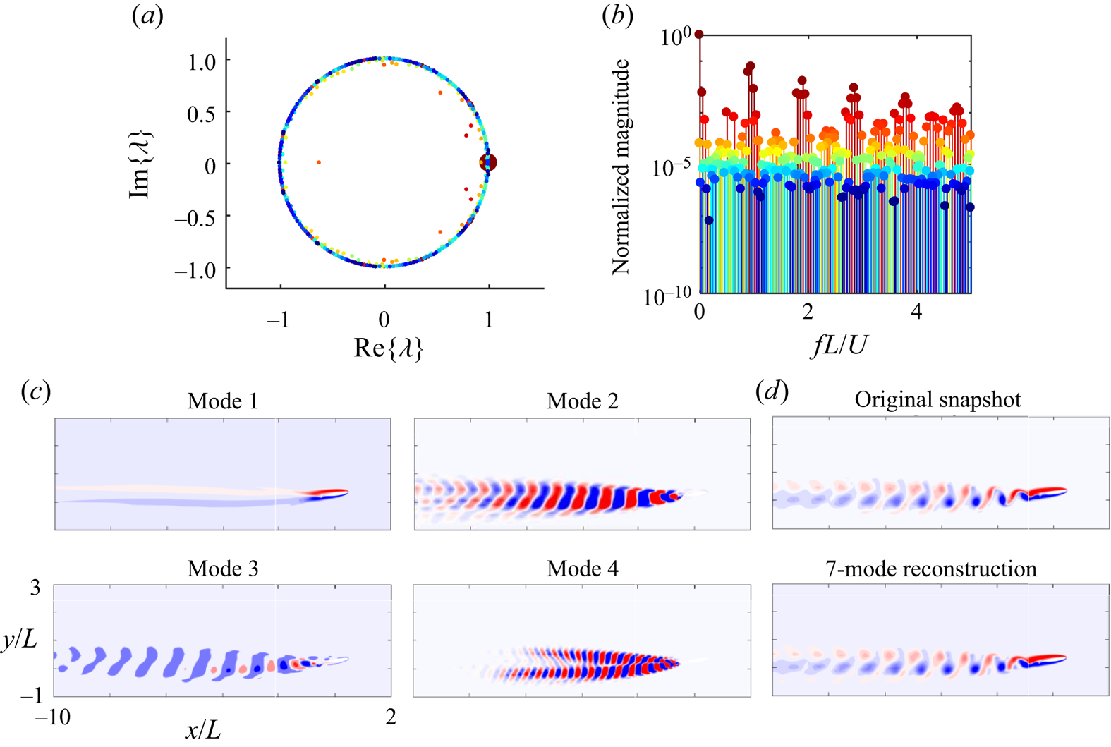
The GW-DMD modes can be utilized to answer the above questions. Figure 23(a) shows the principal eigenvalues (Ritz values) of the GW-DMD modes of the  $St=0.1$ case on the complex plane. The size of the points is scaled based on the magnitude of the corresponding modes, and the colour matches the frequency plot shown in figure 23(b). We should note that only the magnitudes with positive frequencies, i.e.
 $\textrm {Im}[\lambda ]>0$, are presented here. Most of the Ritz values are located on the unit circle
 $|\lambda |=1$, which is expected as the system exhibits an orderly periodic vortex shedding. The four modes corresponding to the largest magnitudes are also plotted in figure 23(c). The one with the largest magnitude has a frequency of
 $St=0$, representing the mean flow field. The second and the fourth modes have frequencies
 $St=0.96$ and
 $St=1.92$, respectively. They are related to the vortex-induced vibration natural frequencies. We will explain what mode 3 represents after looking at the GW-DMD modes of the case with the flapping frequency
 $St=0.9$, shown in figure 24. In this case, most of the Ritz values still fall on the unit circle, indicating these modes do not grow or decay and are, therefore, either stationary or periodic. The first, second and fourth modes are identical to the
 $St=0.1$ case, related to the mean and the natural frequency and its harmonics, respectively. However, the third mode is exceptionally different from the
 $St=0.1$ case. In the
 $St=0.9$ case, the third mode, with frequency
 $St=0.9$, extends further downstream and signifies the vortex shedding caused by the rapid flap motion. When the flap moves downward, it induces large pressure gradient forces on a negative vortex layer on top of the flap. The flow separates but remains close to the upper surface of the trailing edge. When the flap moves upward, the vortex is propelled away. This creates an orderly wake that interacts with the geometry-induced vortex shedding wake structure in mode 2. The interference between these two modes creates the two peaks in the power spectrum at
 $St=0.9$ and
 $St=0.06$ (figure 21). The slight mismatch between the flap- and geometry-induced vortices results in the periodically large-amplitude heaving motion. On the other hand, with the flapping frequency of
 $St=0.1$, the third mode only affects a small region close to the trailing edge. This implies that the slow-moving active flap, in this case, does not induce vortex shedding as the pressure gradient is much weaker. Instead, the movement of the flap modifies the geometry of the system and the departure angle of the geometry-induced wake, resulting in the large-amplitude motion with the same frequency as the flap motion
 $St=0.1$.
(a) The principal eigenvalues, (b) normalized magnitude relative to the frequency of GW-DMD modes, (c) first four modes with the largest magnitudes for case  $St=0.1$ with
 $\alpha =10^\circ$ and
 $A=1.5^\circ$, and (d) the comparison between the reconstructed and original vorticity field.

(a) The principal eigenvalues, (b) normalized magnitude relative to the frequency of GW-DMD modes, (c) first four modes with the largest magnitudes for case  $St=0.9$ with
 $\alpha =10^\circ$ and
 $A=1.5^\circ$, and (d) the comparison between the reconstructed and original vorticity field.

The reconstruction of a selected frame with the first four mode pairs is shown in figures 23(d) and 24(d). The reconstruction is relatively accurate, meaning that the GW-DMD has successfully extracted the dominant dynamic features in both systems.
In this section we demonstrated the capability of GW-DMD modes for isolating important flow features along with their corresponding characteristic frequencies in an FSI system. Similar heaving responses from two cases with different flap frequencies are shown to have inherently different driving mechanisms using the GW-DMD modes. At low frequency, the flap does not induce vortex shedding but changes the direction of the wake. In contrast, at higher flap frequencies the fast structural deformation introduces new vortices to the wake and causes interference between this flap-induced and the geometry-induced wake leading to the periodic motion of the foil. This shows that the proposed method enables a discriminating modal analysis of FSI systems with a simultaneously moving and deforming body. The method can also be employed to extract information not directly available from the structural response or the wake dynamics.
4. Conclusions
In this paper a novel approach is proposed to systematically generate a spatial weighting based on local geometry to enable data-driven modal decomposition techniques for FSI problems involving a deforming and moving body. Through the conformal mapping process, we can map an arbitrary smooth geometry to a unit circle with the mapping incorporated in the Jacobian. We demonstrate how the GW-MD methods can successfully extract characteristic system dynamics with three illustrative examples. The GW-DMD modes can connect the frequency information obtained from the structural motion to flow structures. Besides, the GW-POD modes can be used to efficiently reconstruct the flow field and could serve as a basis for reduced-order modelling.
The GW-MD techniques have the benefits of being readily deployable to any smooth geometry. They can be post applied to experimental or numerical methods providing the geometry is available for the conformal mapping process. However, the method employed here is limited to two-dimensional analysis due to the constraint of much fewer full conformal mappings available at higher dimensions. The current effort explores the possibility of extending the same concept to 3-D geometries using differential geometry techniques. In computational science research quasi-conformal mapping techniques have been used for shape recognition and surface mapping. Among different quasi-conformal techniques, there are methods such as discrete conformal mapping that preserves the angle of the mesh while being Laplacian conservative (Gotsman et al. Reference Gotsman, Gu and Sheffer2003; Floater & Hormann Reference Floater and Hormann2005; Li & Hartley Reference Li and Hartley2007), which is suitable for the current work. Also, harmonic mapping (Yanushauskas Reference Yanushauskas1970; Wang et al. Reference Wang2003) and volume parameterization of three-manifolds with small angular and volume distortions (Paillé & Poulin Reference Paillé and Poulin2012; Kovalsky et al. Reference Kovalsky, Aigerman, Basri and Lipman2015) are promising techniques to extend these analyses to higher dimensions. Advanced methods can also handle deformation in the structure (Zeng & Gu Reference Zeng and Gu2011; Lee, Lam & Lui Reference Lee, Lam and Lui2016), which provides a path to extend the current study. With further development, the current method can be exploited to form ROMs and the subsequent design of control methods for shape-changing FSI problems. Another future direction is to relate interface forces between the solid and fluid to flow field modes using the force partitioning kernel technique (Martín-Alcántara, Fernandez-Feria & Sanmiguel-Rojas Reference Martín-Alcántara, Fernandez-Feria and Sanmiguel-Rojas2015; Zhang, Hedrick & Mittal Reference Zhang, Hedrick and Mittal2015; Moriche, Flores & García-Villalba Reference Moriche, Flores and García-Villalba2017; Wu, Liu & Liu Reference Wu, Liu and Liu2018; Menon & Mittal Reference Menon and Mittal2020b) and essentially extend the modal analysis to solid using these force kernels. The conformal mapping provides a systematic way to investigate the fluid dynamic forces in a spatially fixed domain and retrieve a linear model describing how the structure interacts with the fluid.
The authors hope that the proposed framework opens up the path to systematically analyse FSI problems with deforming geometries and expand the horizon of analysing complex FSI systems.
Funding
This work is supported by the Defense Advanced Research Projects Agency, grant number D19AP00035.
Declaration of interests
The authors report no conflict of interest.
Appendix A. Validation of the algorithm
To validate the numerical algorithm used in this study, we compare our predictions to literature for several benchmark canonical problems.
The first case is a stationary cylinder placed in uniform flow. The Reynolds number  $Re$ is based on the diameter of the cylinder, and the incoming flow speed ranges from 50 to 1000.
The computational grid is set up with the same mapping procedure introduced in § 2, with the resolution  $400\times 512$ in the radial and angular directions, respectively, and extended to 50 diameters of the cylinder. The time interval is chosen to be
 $\Delta t=0.0005$. Figure 25 shows the flow field compared with results from Saiki & Biringen (Reference Saiki and Biringen1996) and Ding et al. (Reference Ding, Shu, Yeo and Xu2007). The present model could correctly replicate the position and intensity of the coherent structure in both Reynolds numbers 100 and 200. The Strouhal number based on the lift, defined as
 $St=fD/U$ with
 $D$ as the diameter of the cylinder, is plotted in figure 26, and compared with the results obtained by other authors experimentally (Roshko Reference Roshko1961) and numerically (Lei, Cheng & Kavanagh Reference Lei, Cheng and Kavanagh2000; Zhao et al. Reference Zhao, Cheng, Teng and Liang2005). Present results agree well with the previously reported numerical results but slightly higher than the experimental results due to the 3-D effect.
Vorticity field behind a cylinder predicted by (a) Saiki & Biringen (Reference Saiki and Biringen1996), (b) Ding et al. (Reference Ding, Shu, Yeo and Xu2007) and (c) the current method.

Strouhal number of the cylinder flow. The two lines indicate the range of experimental results from Roshko (Reference Roshko1961).

The second case is the lift coefficient of a translating ellipsoid at different angles of attack. The canonical problem is compared with the results from Wang (Reference Wang2000) where, as shown in figure 27, a good match is found.
Comparison of the lift coefficient of an ellipsoid at different angles of attack with the literature.

The third case is the dynamic force measurement comparison of a translating and rotating wing described by Wang, Birch & Dickinson (Reference Wang, Birch and Dickinson2004). The ratio of the translational motion amplitude and the chord length is  $A_0/c=2.8$, and there is no phase difference between the translational and rotational motion. The angle of attack is fixed at
 $\alpha _0={\rm \pi} /2$, the amplitude of pitching angle at
 $\beta ={\rm \pi} /4$ and the frequency at
 $f=0.25$. The Reynolds number based on the translational amplitude
 $A_0$ and chord length
 $c$ is 75. Following the definition by Wang et al. (Reference Wang, Birch and Dickinson2004), the forces are normalized with the maximum quasi-steady forces. Figure 28 and table 1 show the comparison of the lift and drag coefficients between current work, both simulation and experimental results provided by Wang et al. (Reference Wang, Birch and Dickinson2004), and numerical results from Eldredge (Reference Eldredge2007). Due to the 3-D effect, none of the numerical results can perfectly replicate the force information acquired from the experiments. However, the maximum value and the overall profile are comparable between the numerical results and the proposed algorithm should be sufficient to support the current work.
Dynamic force coefficients of a flapping elliptic wing.

Statistical comparison of the dynamic force coefficients of a flapping elliptic wing.

Appendix B. Formulation of the modified Navier–Stokes equation in the transformed domain
To solve the Navier–Stokes equation in the transformed space, we need to modify the Navier–Stokes equations accordingly. We follow the procedure introduced by Batchelor (Reference Batchelor2000) to achieve this. The transformation process has two stages: first, the global Cartesian coordinate  $(x, y)$ is transformed into a moving reference frame
 $(X, Y)$ considering the heaving and pitching motion of the structure, then through the conformal mapping procedure
 $(X, Y)$ is transformed into a cylindrical coordinate system
 $r \textrm {e}^{\textrm {i} \phi }$.
A smooth geometry is considered in the Cartesian coordinate system  $(x, y)$. The structure is assumed to have heaving and pitching motion, with the amplitude being
 $h$ and
 $\alpha$, respectively. The Navier–Stokes equations to be solved, represented in the vorticity-stream function
 $(\omega -\psi )$ form, are
 \begin{gather} \frac{\partial\omega}{\partial t}+\frac{\partial\psi}{\partial y} \frac{\partial\omega}{\partial x}-\frac{\partial\psi}{\partial x} \frac{\partial\omega}{\partial y} = \frac{1}{Re}\left[\frac{\partial^2\omega}{\partial x^2}+\frac{\partial^2\omega}{\partial y^2}\right], \end{gather}
 \begin{gather} \frac{\partial^2\psi}{\partial x^2}+\frac{\partial^2\psi}{\partial y^2} = -\omega. \end{gather}
With the coordinate transformation
 \begin{equation} (X,Y) = x(\cos\alpha, -\sin\alpha) + (y-h)(\sin\alpha, \cos\alpha), \end{equation}
we acquire the Navier–Stokes equation in the  $(X, Y)$ domain as
 \begin{gather} \frac{\partial\omega}{\partial t}+U \frac{\partial\omega}{\partial X}+V \frac{\partial\omega}{\partial Y} = \frac{1}{Re}\left[\frac{\partial^2\omega}{\partial X^2}+\frac{\partial^2\omega}{\partial Y^2}\right], \end{gather}
 \begin{gather} \frac{\partial^2\psi}{\partial X^2}+\frac{\partial^2\psi}{\partial Y^2} = -\omega, \end{gather}
where  $U$ and
 $V$ are
 \begin{gather} U = u \cos\alpha+\left(v-\frac{\textrm{d}h}{\textrm{d}t}\right)\sin\alpha+Y\frac{\textrm{d} \alpha}{\textrm{d}t}, \end{gather}
 \begin{gather} V = \left(v-\frac{\textrm{d}h}{\textrm{d}t}\right) \cos\alpha-u \sin\alpha-X\frac{\textrm{d} \alpha}{\textrm{d}t}, \end{gather}
while  $u = \partial \psi /\partial y$ and
 $v=-\partial \psi /\partial x$ are the horizontal and vertical velocities under the
 $(x, y)$ coordinate.
Now we look at the transformation from the  $(X,Y)$ plane to the
 $\zeta =(\xi , \eta )$ plane. We can assume that the transformation and inverse transformation are
 \begin{gather} \xi = f(X,\,Y), \quad \eta = g(X, Y), \end{gather}
 \begin{gather} X = F(\xi , \eta), \quad Y = G(\xi , \eta). \end{gather}
It follows that
 \begin{equation} \left[ \begin{array}{@{}c@{}} \textrm{d}X \\ \textrm{d}Y \end{array} \right] = \left[ \begin{array}{@{}cc@{}} F_\xi & F_\eta \\ G_\xi & G_\eta \end{array} \right] \left[ \begin{array}{@{}c@{}} \textrm{d}\xi \\ \textrm{d}\eta \end{array} \right], \end{equation}
and
 \begin{equation} \left[ \begin{array}{@{}c@{}} \textrm{d}\xi \\ \textrm{d}\eta \end{array} \right] = \dfrac{1}{F_\xi G_\eta-F_\eta G_\xi} \left[ \begin{array}{@{}cc@{}} G_\eta & -F_\eta \\ -G_\xi & F_\xi \end{array} \right] \left[ \begin{array}{@{}c@{}} \textrm{d}X \\ \textrm{d}Y \end{array} \right], \end{equation}
where the subscript variables denote derivation relative to the variable. We define the determinant of the Jacobian to be  $|J|=F_\xi G_\eta - F_\eta G_\xi$. Then we can follow the relations given in Batchelor (Reference Batchelor2000) to calculate the convective term. We have the relation
 \begin{equation} (\textrm{d}X)^2+(\textrm{d}Y)^2 = (F_\xi^2+G_\xi^2)(\textrm{d}\xi)^2 + (F_\eta^2+G_\eta^2)(\textrm{d}\eta)^2+2(F_\xi F_\eta+G_\xi G_\eta)\,\textrm{d}\xi\,\textrm{d}\eta. \end{equation}
Note that since the transformation is conformal, the Cauchy–Riemann relation holds and the last term goes to zero, i.e.  $F_\xi F_\eta +G_\xi G_\eta =0$, and, hence, the scaling factors are
 \begin{gather} h_1 = \sqrt{F_\xi^2+G_\xi^2}=\sqrt{F_\xi G_\eta +G_\xi(-F_\eta)}=\sqrt{|J|}, \end{gather}
 \begin{gather} h_2 = \sqrt{F_\eta^2+G_\eta^2}=\sqrt{F_\eta(-G_\xi) +G_\eta F_\xi}=\sqrt{|J|}. \end{gather}
The unit vectors parallel to the coordinate lines are
 \begin{gather} \tilde{a} = h_1\left(\frac{\partial \xi}{\partial X},\, \frac{\partial \xi}{\partial Y}\right) = \frac{1}{\sqrt{|J|}}\left(\frac{\partial Y}{\partial \eta},\, -\frac{\partial X}{\partial \eta}\right), \end{gather}
 \begin{gather} \tilde{b} = h_2\left(\frac{\partial \eta}{\partial X},\, \frac{\partial \eta}{\partial Y}\right) = \frac{1}{\sqrt{|J|}}\left(-\frac{\partial Y}{\partial \xi},\, \frac{\partial X}{\partial \xi}\right). \end{gather}
We then recover the convective term in the  $(\xi , \eta )$ domain as
 \begin{equation} v\boldsymbol{\cdot}\boldsymbol{\nabla}\omega=(V_\xi, V_\eta)\boldsymbol{\cdot}\left(\frac{\tilde{a}}{h_1}\frac{\partial}{\partial \xi}, \frac{\tilde{b}}{h_2}\frac{\partial}{\partial \eta}\right)\omega. \end{equation}
The Navier–Stokes equations in the  $(\xi , \eta )$ are thus
 \begin{gather} \frac{\partial\omega}{\partial t}+\frac{V_\xi}{\sqrt{|J|}} \frac{\partial\omega}{\partial \xi}+ \frac{V_\eta}{\sqrt{|J|}} \frac{\partial\omega}{\partial \eta} = \frac{1}{Re\,|J|}\left[\frac{\partial^2\omega}{\partial \xi^2}+\frac{\partial^2\omega}{\partial \eta^2}\right], \end{gather}
 \begin{gather} \frac{\partial^2\psi}{\partial \xi^2}+\frac{\partial^2\psi}{\partial \eta^2} = -|J|\omega, \end{gather}
with the  $V_\xi$ and
 $V_\eta$ being
 \begin{gather} V_\xi = \frac{1}{\sqrt{|J|}} \left\{ \left(F_\eta G_t-F_t G_\eta\right) + \left[ \frac{\partial \psi}{\partial \eta} + \left(Y\frac{\textrm{d}\alpha}{\textrm{d}t}-\frac{\textrm{d}h}{\textrm{d}t}\sin\alpha\right)G_\eta \right.\right.\nonumber\\ \left.\left.+\left(X\frac{\textrm{d}\alpha}{\textrm{d}t} +\frac{\textrm{d}h}{\textrm{d}t}\cos\alpha\right)F_\eta \right]\right\}, \end{gather}
 \begin{gather} V_\eta = \frac{1}{\sqrt{|J|}} \left\{ \left(G_\xi F_t - G_t F_\xi\right) + \left[ -\frac{\partial \psi}{\partial \xi} - \left(Y\frac{\textrm{d}\alpha}{\textrm{d}t}-\frac{\textrm{d}h}{\textrm{d}t}\sin\alpha\right) G_\xi \right.\right.\nonumber\\ \left.\left.-\left(X\frac{{\rm d}\alpha}{\textrm{d}t} +\frac{\textrm{d}h}{\textrm{d}t}\cos\alpha\right)F_\xi \right]\right\}. \end{gather}
Finally, we introduce the polar coordinate  $(r,\, \theta )$ in the plane
 $(\xi ,\, \eta )$. The final form of the Navier–Stokes equations in the
 $(r, \theta )$ are thus
 \begin{gather} \frac{\partial\omega}{\partial t}+\frac{1}{\sqrt{|J|}}\left[V_r\frac{\partial\omega}{\partial r}+\frac{V_\theta}{r}\frac{\partial\omega}{\partial\theta}\right]=\frac{1}{Re \, |J|}\left[\frac{\partial^2\omega}{\partial r^2}+\frac{1}{r} \frac{\partial \omega}{\partial r}+\frac{1}{r^2}\frac{\partial^2\omega}{\partial\theta^2}\right], \end{gather}
 \begin{gather} \frac{\partial^2\psi}{\partial r^2}+\frac{1}{r}\frac{\partial\psi}{\partial r}+\frac{1}{r^2}\frac{\partial^2\psi}{\partial\theta^2}=-|J|\omega, \end{gather}
with  $V_r$ and
 $V_\theta$ being
 \begin{gather} V_r = V_\xi \cos\theta +V_\eta \sin\theta, \end{gather}
 \begin{gather} V_\theta = -V_\xi \sin\theta + V_\eta \cos\theta. \end{gather}