1 Introduction
Granular currents are flows of dense granular materials down inclines, driven by gravity and resisted by internal and basal friction. Such materials include sand, gravel, powders and freshly fallen snow, all of which consist of discrete particles. Granular currents include snow avalanches and landslides, which are responsible for over 7000 deaths annually, causing economic and social damage especially in developing countries (Petley Reference Petley2012). To increase our understanding of these devastating flows, and aid with prediction and mitigation, it is essential to develop detailed mathematical models of such flows.
It is often desirable to approximate granular flows as continua. Granular currents in nature tend to be shallow: their depths are small compared to the length scales over which they extend and vary. Continuum models of granular currents commonly exploit this low aspect ratio by using a depth-averaged approach (Savage & Hutter Reference Savage and Hutter1989; Pouliquen & Forterre Reference Pouliquen and Forterre2002; Gray & Edwards Reference Gray and Edwards2014), similar to the shallow water models of hydraulics (Chow Reference Chow1959; Peregrine Reference Peregrine1967). This approach discards information about the depthwise dependence of the flow. These models provide a simple set of governing equations, but they are unsatisfactory when there are topographical features that change the depthwise profile or the flow, affecting the amount of resistance or dissipation experienced by the current.
Depth-averaged models for granular currents typically feature equations for mass and momentum conservation, of the form
 $$\begin{eqnarray}\displaystyle & \displaystyle {\displaystyle \frac{\unicode[STIX]{x2202}h}{\unicode[STIX]{x2202}t}}+{\displaystyle \frac{\unicode[STIX]{x2202}}{\unicode[STIX]{x2202}x}}(h\overline{u})=0, & \displaystyle\end{eqnarray}$$
 $$\begin{eqnarray}\displaystyle & \displaystyle {\displaystyle \frac{\unicode[STIX]{x2202}}{\unicode[STIX]{x2202}t}}(h\overline{u})+{\displaystyle \frac{\unicode[STIX]{x2202}}{\unicode[STIX]{x2202}x}}\left(\frac{1}{2}h\overline{u^{2}}+\frac{1}{2}gh^{2}\cos \unicode[STIX]{x1D703}\right)=gh(\sin \unicode[STIX]{x1D703}-\unicode[STIX]{x1D707}\cos \unicode[STIX]{x1D703})+{\displaystyle \frac{\unicode[STIX]{x2202}}{\unicode[STIX]{x2202}x}}\left(D{\displaystyle \frac{\unicode[STIX]{x2202}\overline{u}}{\unicode[STIX]{x2202}x}}\right),\qquad & \displaystyle\end{eqnarray}$$
 $\unicode[STIX]{x1D703}$
is the inclination,
 $h(x,t)$
is the depth of the current,
 $u(x,z,t)$
is the streamwise velocity and an overbar indicates a depth-average so that, for example,
 $$\begin{eqnarray}\overline{u}=\overline{u}(x,t)=\frac{1}{h(x,t)}\int _{0}^{h}u(x,z,t)\,\text{d}z.\end{eqnarray}$$
Equation (1.1b
) is a depth-integrated momentum balance equation; its right-hand side contains three accelerative terms: gravitational driving
 $gh\sin \unicode[STIX]{x1D703}$
, Coulomb frictional resistance
 $\unicode[STIX]{x1D707}gh\cos \unicode[STIX]{x1D703}$
and a viscous-like term with a possibly variable viscosity
 $D$
. For
 $\unicode[STIX]{x1D703}=\unicode[STIX]{x1D707}=D=0$
, one recovers the Saint-Venant equations governing shallow water flows with negligible viscosity or drag. (For currents on a varying slope it is necessary to introduce extra terms to account for the curvature from non-constant
 $\unicode[STIX]{x1D703}$
.)
In order to close the system (1.1), one must relate
 $\overline{u^{2}}$
,
 $\unicode[STIX]{x1D707}$
and
 $D$
to the dynamical variables
 $h$
and
 $\overline{u}$
. To this end, the
 $\overline{u^{2}}$
term is expressed in terms of
 $\overline{u}$
through a ‘shape factor’ (e.g. Woodhouse, Phillips & Hogg Reference Woodhouse, Phillips and Hogg2016), defined by
 $$\begin{eqnarray}\unicode[STIX]{x1D712}(x,t)=\overline{u^{2}}/\overline{u}^{2}.\end{eqnarray}$$
The shape factor characterises different velocity profiles:
 $\unicode[STIX]{x1D712}=1$
for a uniform (or plug) flow and
 $\unicode[STIX]{x1D712}>1$
for all other profiles. Determining the value of
 $\unicode[STIX]{x1D712}$
is difficult because experimental techniques such as particle image velocimetry (Lueptow, Akonur & Shinbrot Reference Lueptow, Akonur and Shinbrot2000) cannot give any information about the internal velocity profile, only the surface velocity. A common modelling approach is therefore to assume that
 $\unicode[STIX]{x1D712}$
is constant, implying that the internal velocity profile conserves its functional form along the current, such that
 $$\begin{eqnarray}u(x,z,t)=\overline{u}(x,t)S\left(\frac{z}{h(x,t)}\right)\end{eqnarray}$$
for some profile function
 $S$
. Furthermore, many studies take
 $\unicode[STIX]{x1D712}=1$
, which implies a plug flow with
 $S=1$
. When
 $\unicode[STIX]{x1D712}$
is taken to be constant, and further closures have been specified for
 $\unicode[STIX]{x1D707}$
and
 $D$
, the depth-averaged equations have a relatively simple hyperbolic form and may be solved numerically or analytically.
Various closure models for
 $\unicode[STIX]{x1D707}$
and
 $D$
have been proposed (Savage & Hutter Reference Savage and Hutter1991; Gray, Wieland & Hutter Reference Gray, Wieland and Hutter1999; Gray & Edwards Reference Gray and Edwards2014), but all of them assume a velocity profile of the form (1.4) so that
 $\unicode[STIX]{x1D712}$
is constant. Such models do not account for any streamwise changes in the velocity profile, as occurs, for example, when the current experiences inhomogeneities in the streamwise direction due to topographical variation, or changes in the basal boundary conditions.
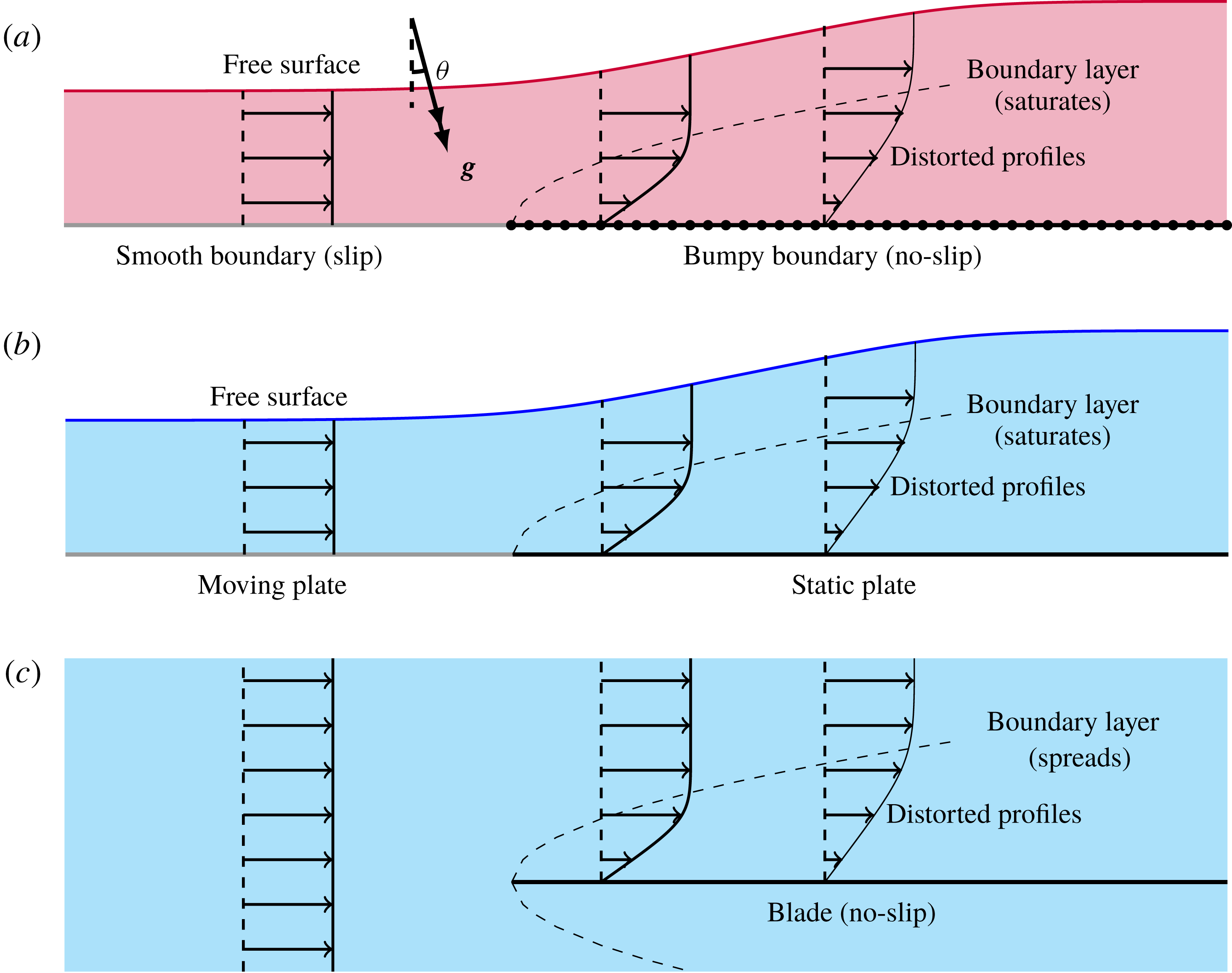
(a) The granular Blasius problem. (b) The free-surface boundary-layer problem studied in Tsang, Dalziel & Vriend (Reference Tsang, Dalziel and Vriend2018). (c) The classical Blasius problem.

In this work, we model the evolution of the velocity profile, and therefore of
 $\unicode[STIX]{x1D712}$
, when a current is subject to a simple change in its basal boundary conditions. We shall study the set-up sketched in figure 1(a). A steady current of a granular material is made to flow first over a surface that is smooth for
 $x<0$
and bumpy for
 $x>0$
, where
 $x$
is a streamwise coordinate. The surface is inclined at constant angle
 $\unicode[STIX]{x1D703}$
to the horizontal, so that the material is driven by a streamwise component of gravity. Individual grains may freely slip along the smooth surface, but the presence of bumpiness causes a transfer of horizontal momentum, reducing the mean streamwise velocity of the grains; in the continuum limit, this can be described as a ‘no-slip’ condition. As illustrated in figure 1, this problem has some similarities to the classical Blasius problem for a Newtonian fluid flow incident onto a blade (Acheson Reference Acheson1990), and we shall refer to it in this article as the ‘granular Blasius problem’. In both problems, the sudden imposition of the no-slip condition for
 $x>0$
causes a distortion in the velocity profile that initially takes place in a narrow boundary layer at the bottom of the flow.
There are three major differences between the classical and the continuum limit of the granular Blasius problems. Firstly, the classical Blasius problem assumes that the blade is immersed in an infinite volume of fluid, but the present problem concerns a current of finite depth, and so a free surface is present, as sketched in figure 1(b). The development of the boundary layer has an effect on the outer flow, displacing the free surface upwards introducing a perturbation to the outer flow, which in turn feeds back on the boundary layer (Tsang et al.
Reference Tsang, Dalziel and Vriend2018). A second difference between the two problems is that the entire system in the granular problem is inclined at an angle
 $\unicode[STIX]{x1D703}>0$
. Gravity therefore drives the flow forwards and opposes the basal drag. The boundary layer does not grow indefinitely but ‘saturates’ when its thickness becomes comparable to that of the current, after which point the current is governed by a balance between gravity and drag, with the incident inertia having been spent. Finally, the Navier–Stokes equations, which govern the classical problem with Newtonian fluids, must be replaced with equations for a rheological model of dense granular flows.
For a rheological model, we use a generalisation of the
 $\unicode[STIX]{x1D707}(I)$
rheology (Jop, Forterre & Pouliquen Reference Jop, Forterre and Pouliquen2006), a model that has successfully described granular currents and associated phenomena, such as granular fingering and roll waves on uniform surfaces (Pouliquen, Delour & Savage Reference Pouliquen, Delour and Savage1997; Gray & Edwards Reference Gray and Edwards2014; Andreotti, Forterre & Pouliquen Reference Andreotti, Forterre and Pouliquen2015; Baker, Johnson & Gray Reference Baker, Johnson and Gray2016). In this work, we shall give analytical solutions to the equations of motion under this rheology, predicting the velocity field inside a granular current, from which the evolution of the shape factor may be found.
We describe the granular Blasius problem in detail in § 2 and give the mathematical formulation in § 3. We then analyse the equations of motion in § 4, eventually providing approximate analytical and numerical solutions for the development of the velocity profile along the current. In § 5 we illustrate the discussion with results from discrete particle model (DPM) simulations, which agree well with the approximate solutions. We discuss the applicability of this work and possible future extensions in §§ 6 and 7.
2 Problem description
We work in two dimensions throughout this article. As noted above, we consider a rigid surface that is inclined at a constant slope
 $\unicode[STIX]{x1D703}$
and use rotated coordinates
 $(x,z)$
, which are taken such that
 $x$
is in the streamwise direction and
 $x$
is perpendicular to the surface. The surface
 $z=0$
is smooth for the region
 $x<0$
, but for
 $x>0$
the surface is made rough using randomly positioned fixed particles of the same size as the grains in the flow. The vectors
 $\hat{\boldsymbol{i}}$
and
 $\hat{\boldsymbol{k}}$
denote the Cartesian unit vectors, and the components of velocity are written as
 $\boldsymbol{u}=u\hat{\boldsymbol{i}}+w\hat{\boldsymbol{k}}$
.
A granular material is introduced at
 $x=x_{min}$
at a constant flow rate
 $q$
, flows down the surface and finally falls off the end of the surface at
 $x=x_{max}$
. Provided that
 $\unicode[STIX]{x1D703}$
lies within a suitable range of values, a statistically steady dense flow will develop. In this steady state, the depth
 $h(x)$
, density
 $\unicode[STIX]{x1D70C}(x,z)$
and velocity
 $(u(x,z),w(x,z))$
are determined.
The behaviour of the flow will depend on the depth
 ${\mathcal{H}}$
and speed
 ${\mathcal{U}}$
of the incident flow. The flow rate, defined as
 $$\begin{eqnarray}q=\int _{0}^{h(x)}u(x,z)\,\text{d}z,\end{eqnarray}$$
is constant and equal to
 ${\mathcal{H}}{\mathcal{U}}$
along the flow, because the flow is steady. This is equivalent to (1.1a
). By analogy with shallow water flows, we define the incident flow’s Froude number as
 $$\begin{eqnarray}Fr=\frac{{\mathcal{U}}}{\sqrt{g{\mathcal{H}}}}.\end{eqnarray}$$
For an inviscid fluid, the Froude number is the ratio of the incident flow velocity to the speed of long (or shallow) waves (Chow Reference Chow1959; Acheson Reference Acheson1990; Billingham & King Reference Billingham and King2001). In this article, we restrict attention to flows with
 $Fr>1$
. Such a flow is said to be ‘supercritical’, and for such flows no linear waves may propagate indefinitely far upstream; consequently, the far-upstream conditions are not affected by any dynamics due to the region
 $x\geqslant 0$
(Tsang et al.
Reference Tsang, Dalziel and Vriend2018). Rather, the values of
 ${\mathcal{H}}$
and
 $q$
may be specified and controlled by some mechanism at
 $x=x_{min}$
, such as a sluice gate. If instead
 $Fr<1$
then it would not be possible to impose these steady upstream conditions. We also assume that the flow remains supercritical after the transition regime, so that the downstream boundary at
 $x=x_{max}$
has only localised effects on the flow.
In the analysis that is to come in § 4, we will in fact assume that
 $Fr\gg 1$
, and find asymptotic solutions that apply in this limit. The limit of high Froude number is relevant for modelling snow avalanches (Hákonardóttir Reference Hákonardóttir2004; Hogg & Jóhannesson Reference Hogg and Jóhannesson2016), but flows at high Froude numbers have proven difficult to implement in laboratory experiments, since it is necessary to have a large quantity of material at hand in order to maintain a fast steady flow (the mechanism described in Holyoake (Reference Holyoake2011) and Holyoake & McElwaine (Reference Holyoake and McElwaine2012) being a notable example of an experimental set-up that provides high-Froude-number flows). Discrete particle method simulations also face difficulties at high Froude numbers, as high-speed collisions in such flows must be resolved using a high particle stiffness, which in turn requires a small time step in order to maintain numerical accuracy.
The actual realisation of a constant depth and flow rate in a DPM simulation is described in § 5.
3 Mathematical formulation
3.1 The
 $\unicode[STIX]{x1D707}(I)$
rheology

The dynamics of granular flows is fundamentally governed by laws on particle collisions and contacts. However, the flows encountered in environmental or industrial applications typically contain huge numbers of irregular grains and it would not be possible to use these microscopic laws to describe the flow as a whole. Instead, we describe the granular flow in terms of continuum fields such as density
 $\unicode[STIX]{x1D70C}(\boldsymbol{x},t)$
and velocity
 $\boldsymbol{u}(\boldsymbol{x},t)$
. These continuum fields represent ensemble averages or local spatial averages of the particle masses, positions and momenta, which are discrete data. The averaging process required to yield a continuum field approximation from a single realisation is known as ‘coarse-graining’ and is defined formally in Weinhart et al. (Reference Weinhart, Hartkamp, Thornton and Luding2013). The density field
 $\unicode[STIX]{x1D70C}$
is sometimes called the ‘bulk density’, to distinguish it from the ‘intrinsic density’
 $\unicode[STIX]{x1D70C}^{\ast }$
of the grains; the ‘packing fraction’ is defined as
 $\unicode[STIX]{x1D719}(\boldsymbol{x},t)=\unicode[STIX]{x1D70C}(\boldsymbol{x},t)/\unicode[STIX]{x1D70C}^{\ast }.$
The continuum laws of mass conservation and momentum balance,
 $$\begin{eqnarray}\displaystyle & \displaystyle {\displaystyle \frac{\unicode[STIX]{x2202}\unicode[STIX]{x1D70C}}{\unicode[STIX]{x2202}t}}+\unicode[STIX]{x1D735}\boldsymbol{\cdot }(\unicode[STIX]{x1D70C}\boldsymbol{u})=0, & \displaystyle\end{eqnarray}$$
 $$\begin{eqnarray}\displaystyle & \displaystyle {\displaystyle \frac{\unicode[STIX]{x2202}\boldsymbol{u}}{\unicode[STIX]{x2202}t}}+\boldsymbol{u}\boldsymbol{\cdot }\unicode[STIX]{x1D735}\boldsymbol{u}=\frac{1}{\unicode[STIX]{x1D70C}}\unicode[STIX]{x1D735}\boldsymbol{\cdot }\unicode[STIX]{x1D748}+\boldsymbol{g}, & \displaystyle\end{eqnarray}$$
 $\unicode[STIX]{x1D748}$
is the Cauchy stress tensor and
 $\boldsymbol{g}$
is the gravitational acceleration (or other body force). We assume that the packing fraction
 $\unicode[STIX]{x1D719}$
and therefore the bulk density
 $\unicode[STIX]{x1D70C}$
are constant, so that (3.1a
) reduces to the incompressibility condition
 $$\begin{eqnarray}\unicode[STIX]{x1D735}\boldsymbol{\cdot }\boldsymbol{u}=0.\end{eqnarray}$$
In reality, granular materials are not incompressible, and a static granular material undergoes Reynolds dilatation when subjected to a shear (da Cruz et al. Reference da Cruz, Emam, Prochnow, Roux and Chevoir2005). Nonetheless, (3.2) appears to be well supported experimentally for steady chute flows (GDR MiDi 2004). Figure 4 of Barker et al. (Reference Barker, Schaeffer, Shearer and Gray2017) shows that the corrections due to compressibility are small except at the free surface. In this article, we are interested in the dynamics at the base of the flow, away from the free surface, so for the analysis in § 4 we assume that (3.2) holds. We note, however, that compressibility is present in our DPM simulations, as will be seen in § 5.1.
As noted in § 1, the problem is not yet closed as we have not yet specified a constitutive relation relating the stress tensor
 $\unicode[STIX]{x1D748}$
to the velocity field
 $\boldsymbol{u}(\boldsymbol{x},t)$
, and boundary conditions on the fields. No universally valid constitutive relation is known for dry granular flows, but the
 $\unicode[STIX]{x1D707}(I)$
rheology (Jop et al.
Reference Jop, Forterre and Pouliquen2006) is the most commonly used model of dense granular flows (Andreotti et al.
Reference Andreotti, Forterre and Pouliquen2015). We summarise it below using our notation, which is based on that of Gray & Edwards (Reference Gray and Edwards2014).
Under the
 $\unicode[STIX]{x1D707}(I)$
rheology, the stress tensor consists of an isotropic part due to pressure
 $p=p(\boldsymbol{x},t)$
and a deviatoric part due to friction. The pressure field is determined from the incompressibility condition (3.2). Similar to the Coulomb friction model, the deviatoric stress has magnitude
 $\unicode[STIX]{x1D707}p$
, where
 $\unicode[STIX]{x1D707}$
is a coefficient of friction, and the deviatoric stress acts in the direction that opposes the strain rate. The full stress tensor is therefore given by
 $$\begin{eqnarray}\unicode[STIX]{x1D748}=p(-\mathbf{1}+\unicode[STIX]{x1D707}\unicode[STIX]{x1D668}),\end{eqnarray}$$
where
 $\mathbf{1}$
is the identity tensor and
 $\unicode[STIX]{x1D668}=\unicode[STIX]{x1D63F}/\Vert \unicode[STIX]{x1D63F}\Vert$
is defined as the ‘shear direction tensor’, with
 $\unicode[STIX]{x1D63F}=(\unicode[STIX]{x1D735}\boldsymbol{U}+\unicode[STIX]{x1D735}\boldsymbol{U}^{\text{T}})/2$
being the strain rate tensor, and the magnitude of a rank 2 tensor defined as
 $\Vert \unicode[STIX]{x1D64F}\Vert =\sqrt{(1/2)\operatorname{trace}(\unicode[STIX]{x1D64F}^{2})}$
. Putting the constitutive relation (3.3) into the momentum equation (3.1b
) gives
 $$\begin{eqnarray}\unicode[STIX]{x1D70C}\frac{\text{D}\boldsymbol{u}}{\text{D}t}=\unicode[STIX]{x1D70C}\boldsymbol{g}-\unicode[STIX]{x1D735}p+\unicode[STIX]{x1D735}\boldsymbol{\cdot }(\unicode[STIX]{x1D707}p\unicode[STIX]{x1D668}),\end{eqnarray}$$
which is analogous to the Navier–Stokes equations for a Newtonian fluid.
The
 $\unicode[STIX]{x1D707}(I)$
rheology is named for its assertion that the coefficient of friction
 $\unicode[STIX]{x1D707}$
is a function solely of the inertial number
 $I$
, defined by
 $$\begin{eqnarray}I=\frac{2d\Vert \unicode[STIX]{x1D63F}\Vert }{\sqrt{p/\unicode[STIX]{x1D70C}}},\end{eqnarray}$$
where
 $d$
is the mean diameter of the grains (and we assume that
 $\unicode[STIX]{x1D70E}_{d}\ll d$
, where
 $\unicode[STIX]{x1D70E}_{d}$
is the standard deviation of particle diameters). This is in contrast to the basic Coulomb friction model, in which
 $\unicode[STIX]{x1D707}$
is constant for a given material. The function
 $\unicode[STIX]{x1D707}(I)$
must be experimentally determined, and depends on the properties of the granular species, such as shape, size dispersity, and intrinsic material properties such as the coefficient of restitution and the contact friction. Mathematical expressions for
 $\unicode[STIX]{x1D707}(I)$
are fitting curves against experimental data, and the most commonly used expression for
 $\unicode[STIX]{x1D707}(I)$
, introduced by Jop, Forterre & Pouliquen (Reference Jop, Forterre and Pouliquen2005) and Jop et al. (Reference Jop, Forterre and Pouliquen2006), is
 $$\begin{eqnarray}\unicode[STIX]{x1D707}(I)=\unicode[STIX]{x1D707}_{1}+\frac{\unicode[STIX]{x1D707}_{2}-\unicode[STIX]{x1D707}_{1}}{I_{0}/I+1}\end{eqnarray}$$
for
 $O(1)$
dimensionless fitting parameters
 $\unicode[STIX]{x1D707}_{1}$
,
 $\unicode[STIX]{x1D707}_{2}$
and
 $I_{0}$
. We shall refer to (3.6) as the Jop fit. Experimental evidence strongly supports an affine dependence of the form
 $\unicode[STIX]{x1D707}(I)\sim \unicode[STIX]{x1D707}_{1}+mI$
for
 $O(1)$
values of
 $I$
, with
 $\arctan (\unicode[STIX]{x1D707}_{1})$
being the dynamic angle of repose of the material. However, the asymptotic behaviour of
 $\unicode[STIX]{x1D707}(I)$
for
 $I\gg 1$
is not determined by current experimental evidence (Saingier, Deboeuf & Lagrée Reference Saingier, Deboeuf and Lagrée2016). We show in § 4.3 that, in the granular Blasius problem, the boundary-layer thickness and velocity profile depend on the asymptotic properties of
 $\unicode[STIX]{x1D707}(I)$
for
 $I\gg 1$
. Crucially, we show in § 4.5 that the asymptotic behaviour embodied in (3.6) does not permit the growing boundary layers that are observed in DPM simulations. We will therefore contend that we must replace (3.6) with an alternative expression for
 $\unicode[STIX]{x1D707}(I)$
, at least for
 $I\gg 1$
.
Writing out (3.4) in components and substituting the appropriate form for
 $\unicode[STIX]{x1D748}$
, one obtains the equations of motion for steady flow
 $$\begin{eqnarray}\displaystyle & \displaystyle u{\displaystyle \frac{\unicode[STIX]{x2202}u}{\unicode[STIX]{x2202}x}}+w{\displaystyle \frac{\unicode[STIX]{x2202}u}{\unicode[STIX]{x2202}z}}=g\sin \unicode[STIX]{x1D703}-{\displaystyle \frac{\unicode[STIX]{x2202}p}{\unicode[STIX]{x2202}x}}+{\displaystyle \frac{\unicode[STIX]{x2202}}{\unicode[STIX]{x2202}x}}(\unicode[STIX]{x1D707}(I)p\unicode[STIX]{x1D634}_{xx})+{\displaystyle \frac{\unicode[STIX]{x2202}}{\unicode[STIX]{x2202}z}}(\unicode[STIX]{x1D707}(I)p\unicode[STIX]{x1D634}_{xz}), & \displaystyle\end{eqnarray}$$
 $$\begin{eqnarray}\displaystyle & \displaystyle u{\displaystyle \frac{\unicode[STIX]{x2202}w}{\unicode[STIX]{x2202}x}}+w{\displaystyle \frac{\unicode[STIX]{x2202}w}{\unicode[STIX]{x2202}z}}=-g\cos \unicode[STIX]{x1D703}-{\displaystyle \frac{\unicode[STIX]{x2202}p}{\unicode[STIX]{x2202}z}}+{\displaystyle \frac{\unicode[STIX]{x2202}}{\unicode[STIX]{x2202}x}}(\unicode[STIX]{x1D707}(I)p\unicode[STIX]{x1D634}_{xz})+{\displaystyle \frac{\unicode[STIX]{x2202}}{\unicode[STIX]{x2202}z}}(\unicode[STIX]{x1D707}(I)p\unicode[STIX]{x1D634}_{zz}), & \displaystyle\end{eqnarray}$$
 $\unicode[STIX]{x1D634}_{ij}$
are the components of the shear direction tensor.
3.2 Boundary conditions
The equations of motion in § 3.1 must be supplemented by boundary conditions on the base and at the free surface.
The free-surface boundary conditions at
 $z=h(x)$
are very similar to those for a Newtonian fluid. For a steady flow, the kinematic boundary condition states that
 $$\begin{eqnarray}u\frac{\text{d}h}{\text{d}x}=w\quad \text{at }z=h(x).\end{eqnarray}$$
When combined with (3.2) and the basal no-penetration condition, discussed below, (3.8) is equivalent to the conservation of flux (2.1). Given the velocity profile
 $u(x,z)$
, (2.1) can be used to calculate the evolution of
 $h(x)$
along the current.
The free-surface dynamic boundary condition
 $\unicode[STIX]{x1D748}\boldsymbol{\cdot }\boldsymbol{n}=\mathbf{0}$
implies that the pressure
 $p$
vanishes on the free surface. The pressure appears in the denominator of the definition (3.5) for the inertial number
 $I$
; to avoid a singular behaviour for
 $I$
, one must also impose the condition that
 $\Vert \unicode[STIX]{x1D63F}\Vert =0$
.
The lower boundary at
 $z=0$
is rigid, so that the no-penetration condition
 $w=0$
applies everywhere on the boundary. The no-slip boundary condition applies for the bumpy region
 $x>0$
, but slip is allowed over the smooth region
 $x<0$
. We must note that, while the no-penetration condition is a kinematic condition, the no-slip condition is a dynamic condition and requires some considerations of the geometry of the basal bumpiness and of the nature of contact forces, especially the frictional interaction between the grains and the wall (Jing et al.
Reference Jing, Kwok, Leung and Sobral2016). The statement that the base is located at
 $z=0$
is an approximation when the base is bumpy, but if the amplitude of the bumps is
 $O(d)$
, rather than
 $O({\mathcal{H}})$
, then the true location of the base may be linearised to
 $z=0$
.
Indeed, the problem as stated is locally ill-posed at
 $x=z=0$
due to the infinite velocity gradient
 $|\unicode[STIX]{x2202}u/\unicode[STIX]{x2202}x|=\infty$
there. We discuss the applicability of the no-slip condition in § 6.1. For now, we note that the DPM simulations in § 5 show that the no-slip condition holds in
 $x>0$
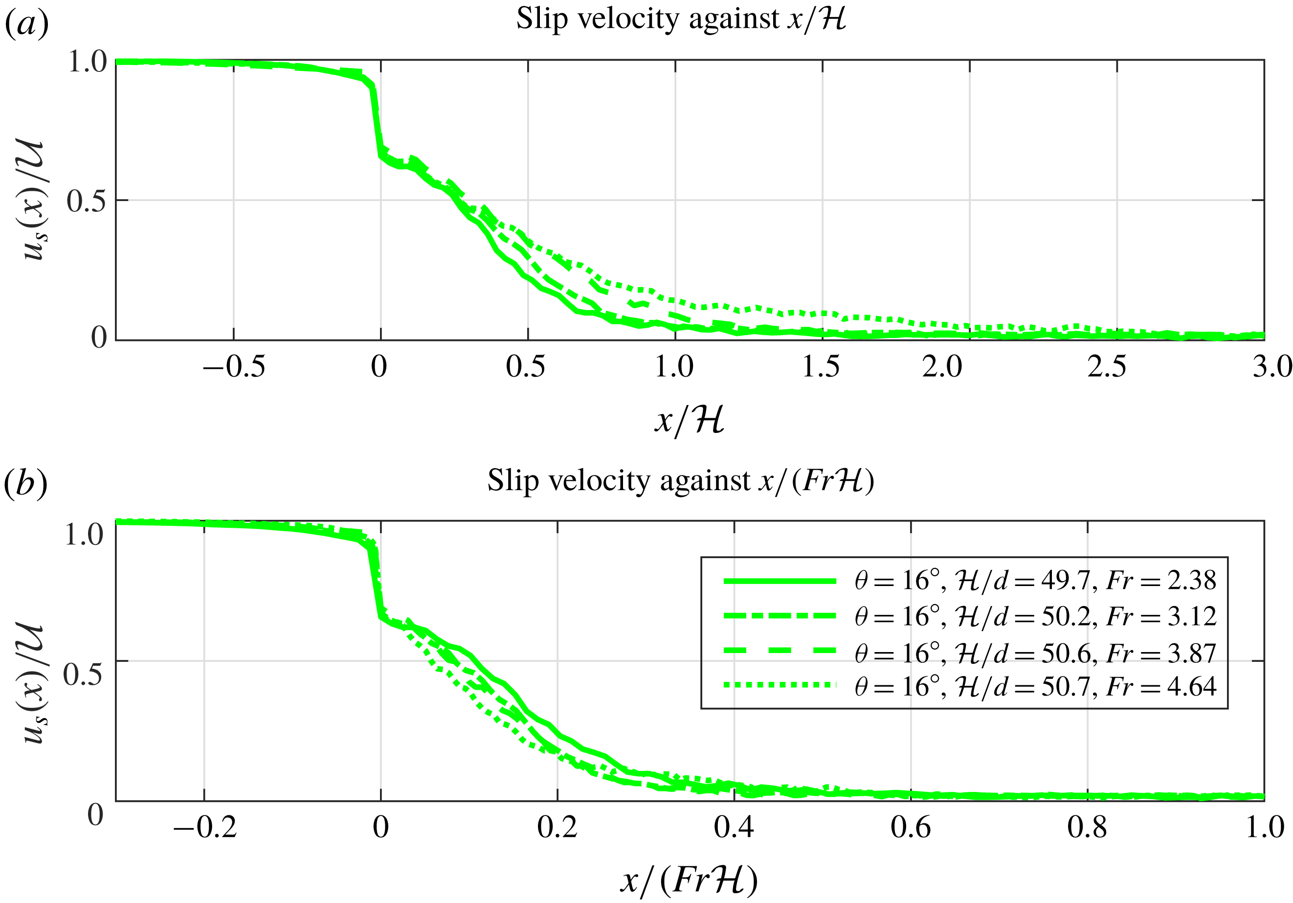
, except within a short transition region, in which the slip velocity decays but does not immediately vanish, as illustrated in figure 6.
4 The depthwise velocity profile
In order to learn about the development of the internal velocity profile of the flow, we now discuss solutions to the
 $\unicode[STIX]{x1D707}(I)$
equations of motion in the limit of high Froude number
 $Fr\gg 1$
. First, in § 4.1 we calculate the flow profiles far upstream and far downstream from the transitional point
 $x=0$
. Then in the following two subsections we study the region in
 $x>0$
in which the flow transitions between its upstream and downstream profiles, on account of the newly imposed no-slip boundary condition. It is here that a boundary layer develops. We find an approximate solution for the boundary-layer velocity profile in § 4.3. Having done that, we consider how the properties of the boundary layer depend on the asymptotic behaviour of the function
 $\unicode[STIX]{x1D707}(I)$
as
 $I\rightarrow \infty$
, and in particular show that the form (3.6) does not permit the formation of a boundary layer.
4.1 Bagnoldian solutions
Consider a shear flow with absolutely no dependence on
 $x$
. The coarsed-grained velocity takes the form
 $\boldsymbol{u}=u(z)\hat{\boldsymbol{i}}$
, and the pressure
 $p=\unicode[STIX]{x1D70C}g(h-z)\cos \unicode[STIX]{x1D703}$
is exactly lithostatic. In this case, the Cauchy momentum equation (3.1b
) together with the constitutive relation (3.3) imply that
 $\unicode[STIX]{x1D707}(I)=\tan \unicode[STIX]{x1D703}$
everywhere.
Following GDR MiDi (2004), we invert for
 $I$
, expand using the definition (3.5) and integrate, obtaining a family of velocity profiles
 $$\begin{eqnarray}u(z)=u_{s}+\frac{2I(\unicode[STIX]{x1D703})}{3d}(g\cos \unicode[STIX]{x1D703})^{1/2}(h^{3/2}-(h-z)^{3/2}),\end{eqnarray}$$
where the slip velocity
 $u_{s}=u(z=0)$
is a constant of integration that parameterises the family of solutions. In this limit of a parallel shear flow, the value of
 $I$
is constant throughout the current and has no dependence on
 $z$
, but is a function of
 $\unicode[STIX]{x1D703}$
, and we have denoted it as
 $I(\unicode[STIX]{x1D703})=\unicode[STIX]{x1D707}^{-1}(\tan \unicode[STIX]{x1D703})$
.
If the no-slip condition is applied at
 $z=0$
, then
 $u_{s}=0$
and (4.1) becomes the celebrated ‘Bagnold velocity profile’ or ‘Bagnoldian velocity profile’ (GDR MiDi 2004), which is analogous to the Nusselt velocity profile of a film of viscous fluid (Ruschak & Weinstein Reference Ruschak and Weinstein2003; Schlichting & Gersten Reference Schlichting and Gersten2017). We refer to the more general form of (4.1) for arbitrary
 $u_{s}$
as a ‘Bagnold-with-slip’ profile. In contrast to the approach for viscous fluids, we do not yet impose the no-slip condition, since it is possible for grains to slide or roll along a wall, even if the contact between them be frictional. Nonetheless, there is a stress between the grains and the wall. As will be shown in § 5.2, a slip velocity is indeed present in
 $x<0$
where the base is smooth. The depth
 $h$
and the slip velocity
 $u_{s}$
are related through the condition (2.1) that the flow rate is
 $q$
, so we may write the slip velocity as a function of depth:
 $$\begin{eqnarray}u_{s}=\frac{q}{h}-\frac{2I(\unicode[STIX]{x1D703})}{5d}(g\cos \unicode[STIX]{x1D703})^{1/2}h^{3/2},\quad I(\unicode[STIX]{x1D703})=\unicode[STIX]{x1D707}^{-1}(\tan \unicode[STIX]{x1D703}).\end{eqnarray}$$
Velocity profiles approximately of the form (4.1) apply when the inertial terms on the left-hand side of (3.7a
) are negligible; for these profiles, the flow is governed internally by a balance between friction and gravity. This is the case sufficiently far from the transition point at
 $x=0$
. An analysis of the depth-averaged equations (1.1) shows that inertial effects decay downstream over a length scale
 $Fr^{2}{\mathcal{H}}$
. Although the flow is downstream, the transition affects the flow just upstream of
 $x=0$
, and it can be shown from (1.1) that the upstream influence affects a region of length scale
 $Fr^{-2}{\mathcal{H}}$
; however, since (1.1) are not valid over streamwise length scales smaller than
 ${\mathcal{H}}$
, we use
 ${\mathcal{H}}$
as a looser bound on the length scale over which upstream influence is present. Therefore, we estimate that Bagnold-with-slip profiles (4.1) hold in the upstream region
 $x\ll -{\mathcal{H}}$
, and the far-downstream region
 $x\gg Fr^{2}{\mathcal{H}}$
.
The far-upstream and far-downstream profiles differ on account of the no-slip condition imposed for
 $x>0$
but not for
 $x<0$
. Far downstream, the no-slip condition
 $u_{s}=0$
applies, so the velocity field adopts the Bagnold profile and the depth is given by the ‘Bagnoldian depth’
 $$\begin{eqnarray}h=h_{Bag}=\left(\frac{5dq}{2I(\unicode[STIX]{x1D703})(g\cos \unicode[STIX]{x1D703})^{1/2}}\right)^{2/5}.\end{eqnarray}$$
Meanwhile, far upstream, a slip velocity is present. The flow far upstream has
 $h={\mathcal{H}}$
by definition, and
 $q={\mathcal{H}}{\mathcal{U}}$
, so
 $u_{s}$
is given by
 $$\begin{eqnarray}u_{s}={\mathcal{U}}-\frac{2I(\unicode[STIX]{x1D703})}{5d}(g\cos \unicode[STIX]{x1D703})^{1/2}{\mathcal{H}}^{3/2}.\end{eqnarray}$$
We assume that the flow rate is sufficiently high that
 $u_{s}>0$
. When it is present, the slip term
 $u_{s}$
in (4.1) adds a uniform speed to the profile. The second term is a velocity gradient due to the shear stress from internal friction. This term is of magnitude
 $O(g^{1/2}{\mathcal{H}}^{3/2}/d)$
. In the limit
 $Fr\gg 1$
with
 $d/{\mathcal{H}}$
fixed, the first term in (4.4) dominates the second. Therefore, in this limit, the incident flow may be approximated as a plug flow.
4.2 The transitional region
$0<x\ll Fr^{2}{\mathcal{H}}$

We next consider the transitional region
 $0<x\ll Fr^{2}{\mathcal{H}}$
. In this region, the inertia terms on the left-hand side of (3.7a
) are not as small and can influence the dynamics of the flow. Therefore, while the far-field dynamics is given by a simple balance between gravity and friction; the transitional region is also affected by the inertia of the current that is carried from upstream.
We shall use an approach similar to Prandtl’s analysis of the classical Blasius problem (Prandtl Reference Prandtl and Krazer1905; Acheson Reference Acheson1990; Schlichting & Gersten Reference Schlichting and Gersten2017), formulated mathematically as the method of matched asymptotic expansions (Hinch Reference Hinch1991). We divide the flow into two regions. The ‘outer layer’ is the main body of the flow, which is largely unaffected by the no-slip condition owing to the inertia of the current. Meanwhile, the newly imposed no-slip boundary condition affects a ‘boundary layer’ near
 $z=0$
, in which the inertia is balanced against friction, so that the no-slip condition may be imposed on the velocity profile.
To leading order we assume that the presence and growth of the boundary layer have no effect on the outer flow, and therefore assume that the outer flow retains its incident depth
 $h={\mathcal{H}}$
and upstream slip velocity
 $u_{s}$
given by (4.4). This assumption is needed to make progress for now, but its validity will be discussed in §§ 4.6 and 6.2. Since the depth is assumed to remain constant at leading order, the pressure
 $p=\unicode[STIX]{x1D70C}g(h-z)\cos \unicode[STIX]{x1D703}$
remains lithostatic, and in particular there is no streamwise pressure gradient at
 $z=0$
. These
 $p$
and
 $u_{s}$
values give matching conditions between the boundary layer and outer problems.
To study the boundary layer, it is expedient to work in terms of non-dimensionalised quantities. We define
 $$\begin{eqnarray}\displaystyle & \displaystyle (x,z,h)=({\mathcal{H}}\tilde{x},\unicode[STIX]{x1D716}{\mathcal{H}}\tilde{z},{\mathcal{H}}\tilde{h}),\quad (u,w)=({\mathcal{U}}\tilde{u} ,\unicode[STIX]{x1D716}{\mathcal{U}}\tilde{w}), & \displaystyle\end{eqnarray}$$
 $$\begin{eqnarray}\displaystyle & \displaystyle (D_{xx},D_{xz},D_{zz})=\frac{{\mathcal{U}}}{{\mathcal{H}}}(\tilde{D}_{xx},\tilde{D}_{xz},\tilde{D}_{zz})=\frac{{\mathcal{U}}}{{\mathcal{H}}}\left({\displaystyle \frac{\unicode[STIX]{x2202}\tilde{u} }{\unicode[STIX]{x2202}\tilde{x}}},\frac{1}{2}\left[\frac{1}{\unicode[STIX]{x1D716}}{\displaystyle \frac{\unicode[STIX]{x2202}\tilde{u} }{\unicode[STIX]{x2202}\tilde{z}}}+\frac{1}{\unicode[STIX]{x1D716}}{\displaystyle \frac{\unicode[STIX]{x2202}\tilde{w}}{\unicode[STIX]{x2202}\tilde{x}}}\right]\!,{\displaystyle \frac{\unicode[STIX]{x2202}\tilde{w}}{\unicode[STIX]{x2202}\tilde{z}}}\right)\!,\; & \displaystyle\end{eqnarray}$$
 $$\begin{eqnarray}\displaystyle & \displaystyle d={\mathcal{H}}\unicode[STIX]{x1D6FF},\quad p=\unicode[STIX]{x1D70C}g{\mathcal{H}}\tilde{p},\quad q={\mathcal{H}}{\mathcal{U}}\tilde{q}, & \displaystyle\end{eqnarray}$$
 $\unicode[STIX]{x1D716}$
is a scaling for the boundary-layer thickness at
 $x={\mathcal{H}}$
, which is to be determined. The actual boundary-layer thickness
 $\unicode[STIX]{x1D6EC}(x)$
will be proportional to
 $\unicode[STIX]{x1D716}$
but will grow with
 $x$
. We assume that
 $\unicode[STIX]{x1D716}\ll 1$
; this will be verified shortly. Note that, for incompressibility (3.2) to be satisfied, the perpendicular velocity
 $w$
must scale as
 $\unicode[STIX]{x1D716}\,{\mathcal{U}}$
.
When these substitutions are made, the incompressibility condition (3.2) reads
 $$\begin{eqnarray}{\displaystyle \frac{\unicode[STIX]{x2202}\tilde{u} }{\unicode[STIX]{x2202}\tilde{x}}}+{\displaystyle \frac{\unicode[STIX]{x2202}\tilde{w}}{\unicode[STIX]{x2202}\tilde{z}}}=0.\end{eqnarray}$$
The streamwise momentum equation (3.7a ) reads
 $$\begin{eqnarray}\displaystyle Fr^{2}\left(\tilde{u} {\displaystyle \frac{\unicode[STIX]{x2202}\tilde{u} }{\unicode[STIX]{x2202}\tilde{x}}}+\tilde{w}{\displaystyle \frac{\unicode[STIX]{x2202}\tilde{u} }{\unicode[STIX]{x2202}\tilde{z}}}\right) & {\sim} & \displaystyle \sin \unicode[STIX]{x1D703}+\frac{1}{\unicode[STIX]{x1D716}}{\displaystyle \frac{\unicode[STIX]{x2202}\tilde{p}}{\unicode[STIX]{x2202}\tilde{z}}}\left(\unicode[STIX]{x1D707}-\frac{1}{2}{\displaystyle \frac{\text{d}\unicode[STIX]{x1D707}}{\text{d}I}}I\right)\nonumber\\ \displaystyle & & \displaystyle +\,\frac{1}{\unicode[STIX]{x1D716}}\tilde{p}{\displaystyle \frac{\text{d}\unicode[STIX]{x1D707}}{\text{d}I}}I\frac{\unicode[STIX]{x2202}^{2}\tilde{u} /\unicode[STIX]{x2202}\tilde{z}^{2}}{\unicode[STIX]{x2202}\tilde{u} /\unicode[STIX]{x2202}\tilde{z}},\end{eqnarray}$$
and the inertial number is
 $$\begin{eqnarray}I=\frac{1}{\unicode[STIX]{x1D716}}\frac{\unicode[STIX]{x1D6FF}Fr}{\tilde{p}^{1/2}}{\displaystyle \frac{\unicode[STIX]{x2202}\tilde{u} }{\unicode[STIX]{x2202}\tilde{z}}},\end{eqnarray}$$
when written in terms of these rescaled quantities. Details of the derivation of (4.7) are given in appendix A. In the above, we have dropped a number of subdominant terms; in particular, the pressure may be treated as being approximately constant across the boundary layer, and
 $\unicode[STIX]{x2202}\tilde{p}/\unicode[STIX]{x2202}\tilde{z}=O(\unicode[STIX]{x1D716})$
. The pressure is therefore given by its lithostatic value from the outer layer,
 $\tilde{p}=\cos \unicode[STIX]{x1D703}$
.
We shall refer to (4.7) as the ‘granular Blasius equation’, governing the velocity in the boundary layer near
 $z=0$
in the transition region. This name reflects its similarity to the classical Blasius equation,
 $$\begin{eqnarray}u{\displaystyle \frac{\unicode[STIX]{x2202}u}{\unicode[STIX]{x2202}x}}+w{\displaystyle \frac{\unicode[STIX]{x2202}u}{\unicode[STIX]{x2202}z}}=-\frac{\text{d}p}{\text{d}x}+\frac{1}{\text{Re}^{2}}{\displaystyle \frac{\unicode[STIX]{x2202}2u}{\unicode[STIX]{x2202}z2}},\end{eqnarray}$$
governing the boundary layer in the classical problem (Schlichting & Gersten Reference Schlichting and Gersten2017). The terms on the right-hand side of (4.9) represent, respectively, the effect of a pressure gradient and of viscosity. Comparing with (4.7), we see that gravity plays the role of a favourable pressure gradient, while friction plays that of an adverse pressure gradient. Meanwhile, the term in (4.7) containing the second derivative (the last term) has a similar effect to the viscous term in (4.9), but it is multiplied by a prefactor that is non-constant but depends on
 $\unicode[STIX]{x2202}u/\unicode[STIX]{x2202}\tilde{z}$
.
In the absence of a rheology, to discriminate between the relative importance of the terms in the general equation (4.7) we need to retain all the terms in (4.7). In the next subsection we introduce a rheology (4.10) in which the first two terms of (4.7), corresponding to the pressure gradient
 $\unicode[STIX]{x2202}p/\unicode[STIX]{x2202}x$
in (4.9), become subdominant, giving a balance between the terms on the left-hand side and the final term on the right-hand side.
4.3 Similarity solutions for the granular boundary layer
When the streamwise pressure gradient term is removed, the classical Blasius equation (4.9) admits a similarity solution and predicts a boundary layer that grows with thickness
 $\unicode[STIX]{x1D6EC}(x)=(x/Re)^{1/2}$
. We now discuss analogous results for the granular Blasius equations (4.6)–(4.8), when suitable approximations are made. Of central importance is the observation that, of the terms on the right-hand side of (4.7), the final ‘viscosity-like’ term is
 $O(1/\unicode[STIX]{x1D716})$
larger than the other two terms. We first find the boundary-layer thickness scaling
 $\unicode[STIX]{x1D716}$
in terms of the other parameters, in such a way that (4.7) admits a dominant balance. We do this by considering the sizes of the terms containing
 $\unicode[STIX]{x1D707}(I)$
and
 $\text{d}\unicode[STIX]{x1D707}/\text{d}I$
.
To make any progress, we must specify the function
 $\unicode[STIX]{x1D707}(I)$
to be used in (4.7). It is evident from (4.8) that the inertial number is large in the boundary layer, on account of the
 $O(1/\unicode[STIX]{x1D716})$
prefactor. This reflects the high shear rate in that layer: the dimensional velocity must adjust from zero at the no-slip boundary to the outer flow’s
 $O({\mathcal{U}})$
slip velocity, over the short depth
 $O(\unicode[STIX]{x1D716}\,{\mathcal{H}})$
. The behaviour of solutions to (4.7) is therefore dependent on the high-
 $I$
asymptotic behaviour of the function
 $\unicode[STIX]{x1D707}(I)$
.
Motivated by the Jop fit (3.6), we consider functions with asymptotic behaviours of the form
 $$\begin{eqnarray}\unicode[STIX]{x1D707}(I)\sim \unicode[STIX]{x1D707}_{s}+mI^{\unicode[STIX]{x1D6FC}}\quad \text{as }I\rightarrow \infty ,\end{eqnarray}$$
where
 $\unicode[STIX]{x1D707}_{s}$
,
 $m$
and the exponent
 $\unicode[STIX]{x1D6FC}$
are constants, with
 $\unicode[STIX]{x1D6FC}m>0$
to ensure that
 $\unicode[STIX]{x1D707}(I)$
increases with
 $I$
; indeed,
 $$\begin{eqnarray}{\displaystyle \frac{\text{d}\unicode[STIX]{x1D707}}{\text{d}I}}I=\unicode[STIX]{x1D6FC}mI^{\unicode[STIX]{x1D6FC}}>0.\end{eqnarray}$$
If
 $\unicode[STIX]{x1D6FC}<0$
, then
 $\unicode[STIX]{x1D707}(I)\rightarrow \unicode[STIX]{x1D707}_{s}$
is bounded as
 $I\rightarrow \infty$
; if
 $\unicode[STIX]{x1D6FC}>0$
, then
 $\unicode[STIX]{x1D707}(I)$
is unbounded. The asymptotic behaviour of (3.6) may be recovered from (4.10) by taking
 $\unicode[STIX]{x1D6FC}=-1$
,
 $m=-(\unicode[STIX]{x1D707}_{2}-\unicode[STIX]{x1D707}_{1})I_{0}<0$
and
 $\unicode[STIX]{x1D707}_{s}=\unicode[STIX]{x1D707}_{2}$
. The form (4.10) has the advantage that
 $\text{d}\unicode[STIX]{x1D707}/\text{d}I$
has a power-law dependence on
 $I$
, so that a similarity solution is possible.
Substituting this form for
 $\unicode[STIX]{x1D707}(I)$
and
 $\text{d}\unicode[STIX]{x1D707}/\text{d}I$
into (4.7), writing
 $I$
out using (4.8) and dropping the subdominant terms, we obtain
 $$\begin{eqnarray}\displaystyle & & \displaystyle Fr^{2}\left(\tilde{u} {\displaystyle \frac{\unicode[STIX]{x2202}\tilde{u} }{\unicode[STIX]{x2202}\tilde{x}}}+\tilde{w}{\displaystyle \frac{\unicode[STIX]{x2202}\tilde{u} }{\unicode[STIX]{x2202}\tilde{z}}}\right)\nonumber\\ \displaystyle & & \displaystyle \quad \sim \,\frac{1}{\unicode[STIX]{x1D716}^{1+\unicode[STIX]{x1D6FC}}}\unicode[STIX]{x1D6FC}m\cos \unicode[STIX]{x1D703}\left[\frac{\unicode[STIX]{x1D6FF}Fr}{(\cos \unicode[STIX]{x1D703})^{1/2}}\right]^{\unicode[STIX]{x1D6FC}}\frac{\unicode[STIX]{x2202}^{2}\tilde{u} /\unicode[STIX]{x2202}\tilde{z}^{2}}{(\unicode[STIX]{x2202}\tilde{u} /\unicode[STIX]{x2202}\tilde{z})^{1-\unicode[STIX]{x1D6FC}}}.\end{eqnarray}$$
The boundary-layer thickness scale
 $\unicode[STIX]{x1D716}$
may be chosen in terms of the other parameters that appear. Taking
 $$\begin{eqnarray}\unicode[STIX]{x1D716}=\left[\frac{\unicode[STIX]{x1D6FC}m\cos \unicode[STIX]{x1D703}}{Fr^{2}}\left[\frac{\unicode[STIX]{x1D6FF}Fr}{(\cos \unicode[STIX]{x1D703})^{1/2}}\right]^{\unicode[STIX]{x1D6FC}}\right]^{1/(1+\unicode[STIX]{x1D6FC})}\end{eqnarray}$$
reduces (4.12) to
 $$\begin{eqnarray}\tilde{u} {\displaystyle \frac{\unicode[STIX]{x2202}\tilde{u} }{\unicode[STIX]{x2202}\tilde{x}}}+\tilde{w}{\displaystyle \frac{\unicode[STIX]{x2202}\tilde{u} }{\unicode[STIX]{x2202}\tilde{z}}}\sim \frac{\unicode[STIX]{x2202}^{2}\tilde{u} /\unicode[STIX]{x2202}\tilde{z}^{2}}{(\unicode[STIX]{x2202}\tilde{u} /\unicode[STIX]{x2202}\tilde{z})^{1-\unicode[STIX]{x1D6FC}}}.\end{eqnarray}$$
We must check whether
 $\unicode[STIX]{x1D716}Fr\ll 1$
, as this assumption is made in the derivation of (4.7), given in appendix A. The conditions under which
 $\unicode[STIX]{x1D716}Fr\ll 1$
are established in appendix B. If
 $\unicode[STIX]{x1D6FC}\geqslant 0$
, then it can be shown that
 $\unicode[STIX]{x1D716}Fr\ll 1$
is satisfied either automatically, or in practice for realistic values of
 $\unicode[STIX]{x1D6FF}$
and
 $Fr$
. For
 $\unicode[STIX]{x1D6FC}<0$
, whether
 $\unicode[STIX]{x1D716}Fr\ll 1$
depends rather strongly on the value of
 $\unicode[STIX]{x1D6FC}$
and the relative sizes of
 $\unicode[STIX]{x1D6FF}$
and
 $Fr$
. As we shall see in § 4.5, the cases
 $\unicode[STIX]{x1D6FC}\leqslant -1$
predict non-physical behaviour for the boundary layer, even if
 $\unicode[STIX]{x1D716}\ll 1$
.
Supplemented by the incompressibility condition, a similarity solution to (4.14) may be found, using techniques similar to those for the classical Blasius problem. This solution takes the form
 $$\begin{eqnarray}\tilde{u} =f^{\prime }(\unicode[STIX]{x1D701}),\quad \unicode[STIX]{x1D701}=\tilde{x}^{-1/(1+\unicode[STIX]{x1D6FC})}\tilde{z},\end{eqnarray}$$
where
 $f$
is the solution to the boundary value problem
 $$\begin{eqnarray}f^{\prime \prime \prime }+\frac{1}{1+\unicode[STIX]{x1D6FC}}(f^{\prime \prime })^{2-\unicode[STIX]{x1D6FC}}f=0,\quad f(0)=f^{\prime }(0)=0,\quad \lim _{\unicode[STIX]{x1D701}\rightarrow \infty }f^{\prime }(\unicode[STIX]{x1D701})=1,\end{eqnarray}$$
with the boundary conditions at
 $\unicode[STIX]{x1D701}=0$
imposing the no-penetration and no-slip conditions, and the condition as
 $\unicode[STIX]{x1D701}\rightarrow \infty$
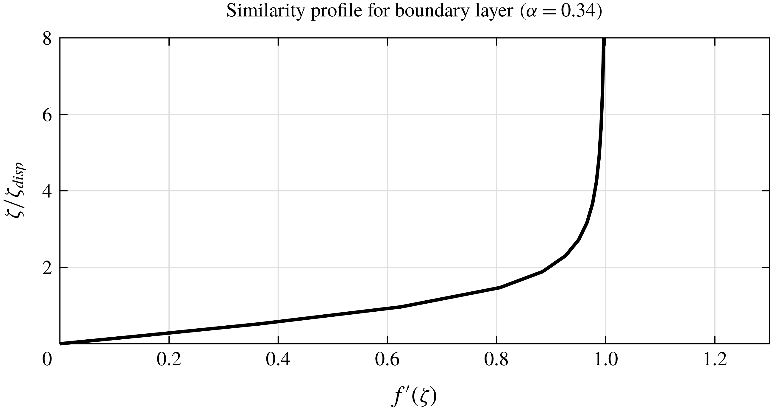
ensuring that the matching condition be satisfied. The numerical solution to (4.16) with
 $\unicode[STIX]{x1D6FC}=0.34$
is shown in figure 2. This value of
 $\unicode[STIX]{x1D6FC}$
is appropriate for our DPM simulations (see table 1). Note the rescaling on the vertical axis: when visually inspecting the thickness of a boundary layer from simulation or experimental results, it is convenient to quote the boundary-layer thickness in terms of the ‘displacement thickness’
 $\unicode[STIX]{x1D701}_{disp}\unicode[STIX]{x1D6EC}(x)$
, where
 $$\begin{eqnarray}\unicode[STIX]{x1D701}_{disp}=\lim _{\unicode[STIX]{x1D701}\rightarrow \infty }(\unicode[STIX]{x1D701}-f(\unicode[STIX]{x1D701})).\end{eqnarray}$$
For
 $\unicode[STIX]{x1D6FC}=0.34$
, the numerical solution to (4.16) has
 $\unicode[STIX]{x1D701}_{disp}\approx 4.35$
.
Numerical solution to (4.16) for
 $\unicode[STIX]{x1D6FC}=0.34$
. The vertical axis has been rescaled by
 $\unicode[STIX]{x1D701}_{disp}\approx 4.35$
to make visual inspection more convenient. The solution was found using the shooting method, with
 $f^{\prime \prime }(0)\approx 0.164$
.

Fitting parameters for the three fits to
 $\unicode[STIX]{x1D707}(I)$
, as shown in figure 5(a).

Reverting to dimensional coordinates, the similarity solution shows that the boundary-layer thickness
 $\unicode[STIX]{x1D6EC}(x)$
is given by
 $$\begin{eqnarray}\unicode[STIX]{x1D6EC}(x)=\unicode[STIX]{x1D716}{\mathcal{H}}\left(\frac{x}{{\mathcal{H}}}\right)^{1/(1+\unicode[STIX]{x1D6FC})}.\end{eqnarray}$$
Moreover, from (4.13), we have
 $$\begin{eqnarray}\unicode[STIX]{x1D716}\propto (d^{\unicode[STIX]{x1D6FC}}g^{1-\unicode[STIX]{x1D6FC}/2}{\mathcal{U}}^{-(2-\unicode[STIX]{x1D6FC})}{\mathcal{H}}^{1-3\unicode[STIX]{x1D6FC}/2})^{1/(1+\unicode[STIX]{x1D6FC})},\end{eqnarray}$$
after dropping
 $O(1)$
non-dimensional constants, and so
 $$\begin{eqnarray}\unicode[STIX]{x1D6EC}(x)\propto (d^{\unicode[STIX]{x1D6FC}}g^{1-\unicode[STIX]{x1D6FC}/2}{\mathcal{U}}^{-(2-\unicode[STIX]{x1D6FC})}{\mathcal{H}}^{1-\unicode[STIX]{x1D6FC}/2}x)^{1/(1+\unicode[STIX]{x1D6FC})}.\end{eqnarray}$$
In the next two subsections we will explore two specific cases for the exponent
 $\unicode[STIX]{x1D6FC}$
.
4.4 The case
$\unicode[STIX]{x1D6FC}=1$

As previously mentioned, the value of
 $\unicode[STIX]{x1D6FC}$
is a fitting parameter for empirical data on the behaviour of the function
 $\unicode[STIX]{x1D707}(I)$
. The case
 $\unicode[STIX]{x1D6FC}=1$
is not necessarily consistent with any particular granular material, but we consider it here for demonstration purposes, since the above discussion is particularly simple in this case.
Suppose that
 $\unicode[STIX]{x1D6FC}=1$
, so that
 $\unicode[STIX]{x1D707}(I)$
takes the affine form
 $$\begin{eqnarray}\unicode[STIX]{x1D707}(I)\sim \unicode[STIX]{x1D707}_{s}+mI\quad \text{as }I\rightarrow \infty .\end{eqnarray}$$
The boundary-layer equation (4.12) reduces to
 $$\begin{eqnarray}\tilde{u} {\displaystyle \frac{\unicode[STIX]{x2202}\tilde{u} }{\unicode[STIX]{x2202}\tilde{x}}}+\tilde{w}{\displaystyle \frac{\unicode[STIX]{x2202}\tilde{u} }{\unicode[STIX]{x2202}\tilde{z}}}\sim {\displaystyle \frac{\unicode[STIX]{x2202}2\tilde{u} }{\unicode[STIX]{x2202}\tilde{z}2}}.\end{eqnarray}$$
This takes exactly the same form as the classical Blasius equation (4.9) for zero streamwise pressure gradient. The boundary-layer thickness scale
 $\unicode[STIX]{x1D716}$
is calculated from (4.13) as
 $$\begin{eqnarray}\unicode[STIX]{x1D716}=\left[\frac{m(\cos \unicode[STIX]{x1D703})^{1/2}\unicode[STIX]{x1D6FF}}{Fr}\right]^{1/2},\end{eqnarray}$$
and the boundary value problem (4.16) becomes
 $$\begin{eqnarray}f^{\prime \prime \prime }+\frac{1}{2}ff^{\prime \prime }=0,\quad f(0)=f^{\prime }(0)=0,\quad \lim _{\unicode[STIX]{x1D701}\rightarrow \infty }f^{\prime }(\unicode[STIX]{x1D701})=1,\end{eqnarray}$$
which governs the velocity profile of the classical Blasius boundary layer in the absence of a pressure gradient (Prandtl Reference Prandtl and Krazer1905; Acheson Reference Acheson1990). The boundary-layer thickness
 $\unicode[STIX]{x1D6EC}(x)$
is given by
 $$\begin{eqnarray}\left.\begin{array}{@{}c@{}}\displaystyle \begin{array}{@{}rcl@{}}\displaystyle \unicode[STIX]{x1D6EC}(x)/{\mathcal{H}}\, & =\, & \displaystyle \unicode[STIX]{x1D716}\tilde{x}^{1/2}\\ \, & =\, & \displaystyle \frac{1}{(\cos \unicode[STIX]{x1D703})^{1/4}}\left(\frac{m\unicode[STIX]{x1D6FF}}{Fr}\tilde{x}\right)^{1/2},\end{array}\\ \displaystyle \unicode[STIX]{x1D6EC}(x)=({\mathcal{H}}x/Re_{GB})^{1/2}.\end{array}\right\}\end{eqnarray}$$
Here
 $$\begin{eqnarray}Re_{GB}=\frac{Fr(\cos \unicode[STIX]{x1D703})^{1/2}}{m\unicode[STIX]{x1D6FF}}=\frac{{\mathcal{U}}{\mathcal{H}}^{1/2}(\cos \unicode[STIX]{x1D703})^{1/2}}{mg^{1/2}d},\end{eqnarray}$$
which we term the ‘granular Blasius Reynolds number’, plays the role that had been played by the Reynolds number in determining the boundary-layer thickness in the classical problem.
In summary, the
 $\unicode[STIX]{x1D707}(I)$
rheology with the linear asymptotic behaviour (4.21) predicts a boundary layer with the same profile and the same
 $x^{1/2}$
scaling as the classical Blasius boundary layer, in the transitional region
 $0<x\ll Fr^{-2}$
where the outer layer may be treated as uniform.
4.5 The cases
$\unicode[STIX]{x1D6FC}\leqslant -1$

The case
 $\unicode[STIX]{x1D6FC}=-1$
is the asymptotic behaviour of the Jop fit (3.6). However, in contrast to the
 $\unicode[STIX]{x1D6FC}=1$
case in the previous subsection, the cases
 $\unicode[STIX]{x1D6FC}\leqslant -1$
do not give physically reasonable similarity solutions for the boundary-layer profile.
With
 $\unicode[STIX]{x1D6FC}=-1$
, the exponent of
 $x$
in (4.18) takes the undefined value of
 $1/0$
. Moreover, for
 $\unicode[STIX]{x1D6FC}<-1$
, the boundary-layer thickness (4.18) decays with
 $x$
. This behaviour is qualitatively distinct from the solution found in the preceding subsection, from the results of DPM simulations and from what we might intuitively expect, in which the boundary thickness grows with
 $x$
. The non-existence of physically realistic similarity solutions for
 $\unicode[STIX]{x1D6FC}\leqslant -1$
should nonetheless be interpreted with caution: the non-existence of a similarity solution does not imply that no solution exists at all.
Further investigation shall be needed to determine whether the cases
 $\unicode[STIX]{x1D6FC}\leqslant -1$
admit any non-self-similar solutions that correctly describe the boundary-layer growth. Although the form (3.6) was chosen as a convenient fitting curve, and although it might have seemed reasonable that the exact mathematical form of such a fitting curve should have no effect on the qualitative behaviour of the system, the analysis of the present section shows that this may not be the case. Therefore, future work should also aim to establish why the non-existence of a similarity solution should be specific to the case
 $\unicode[STIX]{x1D6FC}=-1$
.
4.6 Evolution of the shape factor
As discussed in § 1, our motivation for this work was to study the evolution of the velocity profile along the current after a point of transition, and in particular to find the evolution of the shape factor
 $\unicode[STIX]{x1D712}$
, defined in (1.3). For a fixed flow rate
 $q$
, the shape factor may be written as
 $$\begin{eqnarray}\unicode[STIX]{x1D712}=\frac{h(x)}{q^{2}}\int _{0}^{h(x)}u(x,z)^{2}\,\text{d}z.\end{eqnarray}$$
In the preceding subsections we have given asymptotic descriptions for the velocity profile throughout the current for
 $Fr^{2}\gg 1$
, which may be summarised as follows. The incoming flow velocity profile is Bagnold-with-slip. For high
 $Fr$
, the slip velocity is large compared to the Bagnoldian velocity, and the incident profile is approximately a plug flow, with
 $\unicode[STIX]{x1D712}\sim 1$
. The shape factor increases throughout the transitional regime
 $0<x\ll Fr^{2}$
as the velocity profile evolves between the far-upstream and far-downstream behaviours. Within this transitional region, the velocity profile may be divided into a boundary layer, in which basal friction resists the inertia of the incident flow, and an outer layer. The boundary layer has a self-similar profile (§ 4.3) with a thickness that grows according to (4.18). The outer layer initially remains plug-like, but experiences a perturbation flow from the growth of the boundary layer, described in § 6.2. Eventually, the boundary layer saturates as its thickness becomes comparable to that of the whole current. After saturation, the entire current is then governed by a balance between basal friction and gravity, with the inertia of the incident flow having been spent. The velocity profile is then Bagnoldian without slip, and so
 $\unicode[STIX]{x1D712}\rightarrow 5/4$
as
 $x\rightarrow \infty$
. As illustration, figure 8 illustrates the evolution of velocity profiles using data from our DPM simulations, described in § 5.
An exact formula for the growth of the shape factor cannot be obtained without calculating the perturbation to the outer flow induced by the boundary layer. Following the notation of Tsang et al. (Reference Tsang, Dalziel and Vriend2018), let the perturbation flow at leading order in
 $\unicode[STIX]{x1D716}$
be denoted as
 $(\unicode[STIX]{x1D716}u^{(1)},\unicode[STIX]{x1D716}w^{(1)})$
, and the perturbation depth and pressure as
 $\unicode[STIX]{x1D716}h^{(1)}$
and
 $\unicode[STIX]{x1D716}p^{(1)}$
, respectively. These perturbations were calculated for a Newtonian current in Tsang et al. (Reference Tsang, Dalziel and Vriend2018): in that problem,
 $w^{(1)}$
satisfies
 $\unicode[STIX]{x1D6FB}^{2}w^{(1)}=0$
and exact solutions may be found in terms of Fourier integrals and special functions. The same calculation under the
 $\unicode[STIX]{x1D707}(I)$
rheology is outside the scope of the present article, as the perturbation variables here satisfy a more complicated system of equations, given in appendix C, which cannot be solved analytically. The equations are nonetheless semilinear, and by scaling arguments we may estimate the growth of
 $\unicode[STIX]{x1D712}$
from the approximate solution found in § 4.3. The boundary-layer thickness (4.25) and the incompressibility condition (4.6) together imply that the perpendicular displacement velocity from the boundary layer has magnitude
 $$\begin{eqnarray}\unicode[STIX]{x1D716}w^{(1)}=O({\mathcal{U}}\unicode[STIX]{x1D6EC}(x)/x)=O(\unicode[STIX]{x1D716}(x/{\mathcal{H}})^{-\unicode[STIX]{x1D6FC}/(1+\unicode[STIX]{x1D6FC})}).\end{eqnarray}$$
This displacement velocity is transmitted into the outer flow
 $w^{(1)}$
. By (3.2), the streamwise perturbation flow in the outer layer is of magnitude
 $$\begin{eqnarray}\unicode[STIX]{x1D716}u^{(1)}=O(\unicode[STIX]{x1D716}w^{(1)}x/{\mathcal{H}})=O(\unicode[STIX]{x1D716}(x/{\mathcal{H}})^{1/(1+\unicode[STIX]{x1D6FC})}),\end{eqnarray}$$
this perturbation being negative as the flow is decelerating. The kinematic free-surface boundary condition (3.8) implies that
 $$\begin{eqnarray}h^{\prime }(x)=O(\unicode[STIX]{x1D716}(x/{\mathcal{H}})^{-\unicode[STIX]{x1D6FC}/(1+\unicode[STIX]{x1D6FC})}),\quad \text{so that }h(x)/{\mathcal{H}}=1+c\unicode[STIX]{x1D716}(x/{\mathcal{H}})^{1/(1+\unicode[STIX]{x1D6FC})}+o(\unicode[STIX]{x1D716}),\end{eqnarray}$$
for some constant
 $c$
. Together, these imply that
 $$\begin{eqnarray}\unicode[STIX]{x1D712}-1\propto \unicode[STIX]{x1D716}(x/{\mathcal{H}})^{1/(1+\unicode[STIX]{x1D6FC})},\end{eqnarray}$$
as the incident flow has shape factor
 $1$
, assuming that the Froude number is high enough that the slip velocity dominates any internal profile.
Although we do not have the constant of proportionality, this knowledge of
 $\unicode[STIX]{x1D712}$
is nonetheless useful for improving a depth-averaged model (1.1b
). Using (4.31),
 $\overline{u^{2}}$
may be expressed as
 $$\begin{eqnarray}\overline{u^{2}}=(1+c\unicode[STIX]{x1D716}(x/{\mathcal{H}})^{1/(1+\unicode[STIX]{x1D6FC})})\overline{u}^{2},\end{eqnarray}$$
where
 $c$
is the unknown constant of proportionality. This result may be useful for depth-averaged modelling of more general topography in which an abrupt change in basal roughness is present.
5 Discrete particle model simulations
The continuum models developed above may be validated by comparison with empirical results. It is difficult to obtain information about the internal structure of a velocity profile in a laboratory experiment, so we resort to DPM simulations (O’Sullivan Reference O’Sullivan2014). For this we use the software package MercuryDPM (Thornton et al. Reference Thornton, Weinhart, Luding and Bokhove2012, Reference Thornton, Krijgsman, te Voortwis, Ogarko, Luding, Fransen, Gonzalez, Bokhove, Imole and Weinhart2013; Weinhart et al. Reference Weinhart, Thornton, Luding and Bokhove2012, Reference Weinhart, Tunuguntla, Lantman, van Schrojenstein, Windows-Yule, Polman, Tsang, Jin, Orefice and van der Vaart2017).
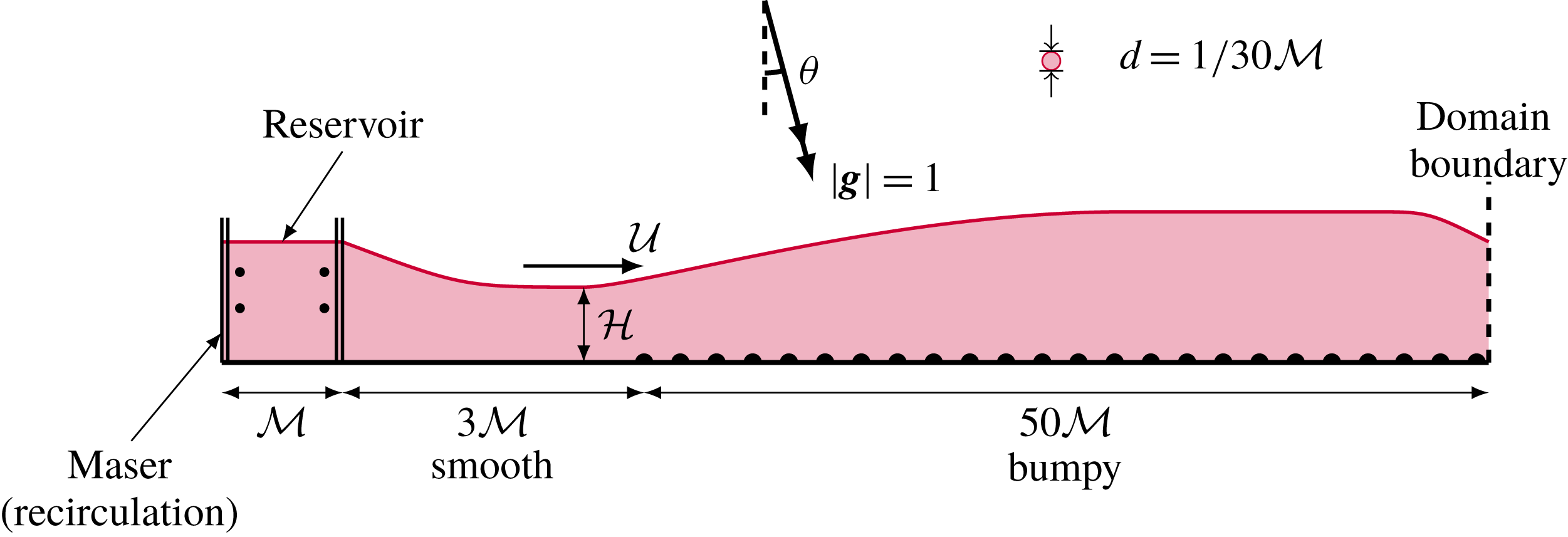
A sketch (not to scale) of the set-up for DPM simulations.

We present a series of DPM simulations in two dimensions, using the set-up sketched in figure 3. The particles are introduced from a reservoir by means of a recirculating system known as a ‘Maser’ (Weinhart et al.
Reference Weinhart, Tunuguntla, Lantman, van Schrojenstein, Windows-Yule, Polman, Tsang, Jin, Orefice and van der Vaart2017; Denissen et al.
Reference Denissen, Weinhart, Voortwis, Luding, Gray and Thornton2019). The Maser consists of two edges, separated by a length
 ${\mathcal{M}}$
, marked in figure 3 as a pair of repeat signs. When a particle is introduced at the right-hand edge, leaving the reservoir, a copy of the particle is introduced at the left-hand edge. The speed of the particles inside this reservoir is kept constant by applying a drag force that counteracts the acceleration due to gravity. The slope
 $\unicode[STIX]{x1D703}$
, the depth of the reservoir and the incident speed are varied.
The reservoir is placed on a smooth boundary at a distance
 $3{\mathcal{M}}$
upstream of the transition point
 $x=0$
. Particles are deleted as they cross the boundary at
 $x=50{\mathcal{M}}$
: this is chosen to be at least
 $2.5Fr^{2}{\mathcal{H}}$
for all the cases that we study. This deletion boundary influences the flow immediately upstream of it, but convergence studies show that, provided
 $Fr$
is sufficiently high, the flow towards the end of the chute is supercritical, and so the effects from the deletion boundary are localised. Since we are instead interested in the region near the transition, we are not concerned as to whether the deletion boundary faithfully represents the end effects of a chute flow.
In these simulations, the depths of these currents are usually
 ${\mathcal{H}}\approx 50d$
. A smaller value of
 $d/{\mathcal{H}}$
would make the continuum approximation more appropriate, but this was too computationally costly. The bumpy base
 $z=0$
for
 $x>0$
is generated by fixing half-discs, all of diameter
 $d={\mathcal{M}}/30$
and of the same material as the moving discs, to the base. The
 $n$
th particle forming the rough base (
 $n=1,2,3,\ldots$
) has its centre at
 $$\begin{eqnarray}(x_{n},z_{n})=\left(4dn,\frac{d}{2}[\tanh (x_{n}/{\mathcal{M}})-1]\right),\end{eqnarray}$$
so that they are spaced equally in the
 $x$
-direction. The ‘mollification’ provided by the
 $\tanh$
profile partially addresses the ill-posedness mentioned in § 3.2: instead of imposing a sudden no-slip condition, the roughness is gradually introduced so that the flow slows down gradually, as shown in figure 6 and discussed in § 5.2.
The value of
 ${\mathcal{U}}$
is defined as the maximum slip velocity in the region
 $x<0$
, and the value of
 ${\mathcal{H}}$
is defined as the depth of the current at that position. Note that
 ${\mathcal{U}}$
and
 ${\mathcal{H}}$
depend on the distance of the reservoir from the transition point, since the flow accelerates and thins in the region
 $x<0$
. The depth and velocity in the reservoir may be controlled exactly, but
 ${\mathcal{H}}$
and
 ${\mathcal{U}}$
are controlled only indirectly.
In these simulations, we shall work in units in which
 ${\mathcal{M}}=1$
and
 $g=1$
; in these units, the time unit is
 $({\mathcal{M}}/g)^{1/2}$
. The simulations reach a quasi-steady state after running for a duration of
 $T=45$
. They are then allowed to run for a further duration
 $\unicode[STIX]{x0394}T=40$
in this steady state, during which time-averaged quantities were computed (sampled at intervals of 0.5). To verify that the flow is quasi-steady, the variations of
 $h$
and
 $\unicode[STIX]{x1D712}$
with time, sampled at a particular point
 $x=10$
, are shown in figure 4 for four different runs. Although the flow is quasi-steady, there is some variability with time, which can be quantified as a Reynolds stress (Hinze Reference Hinze1975), defined in appendix D. Reynolds stress has the same dimensions of momentum flux. As we show in appendix D, the trace of the Reynolds stress is small compared to the time-averaged momentum flux, confirming that the assumption of quasi-steadiness is acceptable.
A plot of (a)
 $h/{\mathcal{M}}$
and (b)
 $\unicode[STIX]{x1D712}$
against time
 $(g/{\mathcal{M}})^{1/2}t$
, sampled at
 $x=10{\mathcal{M}}$
, for four different settings of
 $\unicode[STIX]{x1D703}$
and
 ${\mathcal{H}}$
.

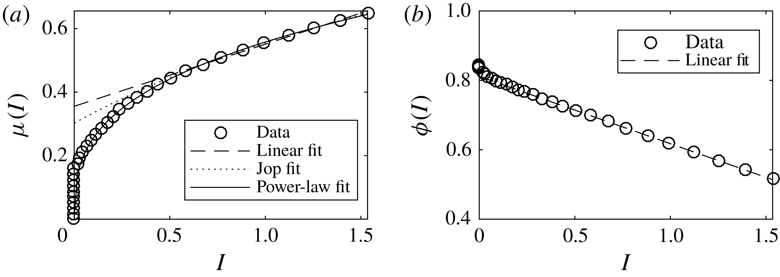
(a) Results from calibration tests (see text) for the function
 $\unicode[STIX]{x1D707}(I)$
for the particles used in our DPM simulations, together with linear (4.21), Jop (3.6) and power-law (4.10) fitting curves, fitted for
 $I>0.5$
. The fitting parameters are shown in table 1. (b) The packing fraction
 $\unicode[STIX]{x1D719}$
against
 $\unicode[STIX]{x1D703}$
, together with the linear best fit
 $\unicode[STIX]{x1D719}(I)=0.81-0.19I$
for
 $I>0.5$
.

In § 5.1 we state the details of the particle-to-particle interactions, and determine the function
 $\unicode[STIX]{x1D707}(I)$
for these particles, as well as assessing the incompressibility assumption (3.2). In § 5.2 we check the validity of the no-slip boundary condition. In § 5.3 we verify that the DPM simulations demonstrate the predicted self-similarity in the boundary layer when the Froude number is sufficiently high. Finally, in § 5.4 we consider the evolution of the outer flow, and therefore the growth of the shape factor.
5.1 Material properties
Particle interactions in these simulations are governed by a linear spring–dashpot (viscoelastic) model, with a coefficient of restitution of
 $0.1$
. There are no grain-to-grain tangential forces: energy is dissipated through the inelasticity of grain-to-grain contacts, rather than by friction. The coefficient of restitution is rather lower than that of real collisions between sand or glass, but the increased dissipation compensates for the two-dimensional geometry of the simulations, in which fewer collisions occur compared to a three-dimensional system. Rajchenbach (Reference Rajchenbach2005) has noted that in a dense flow, the rheological behaviour is independent of the coefficient of restitution, due to the large number of contacts and because grains remain in contact with each other for long periods of time.
In order to compare simulation results against the predictions of the
 $\unicode[STIX]{x1D707}(I)$
rheology, we need to determine the function
 $\unicode[STIX]{x1D707}(I)$
for the materials used in these simulations. We note that the quantity
 $\unicode[STIX]{x1D707}(I)$
expresses the bulk friction of the material, which is non-zero despite individual contacts being frictionless. The calibration of
 $\unicode[STIX]{x1D707}(I)$
is based on a set-up by GDR MiDi (2004). We let the discs flow under gravity in a sloped periodic domain with a bumpy base, and measure the steady flow rate that develops as a function of the slope
 $\unicode[STIX]{x1D703}$
. In a steady flow,
 $\unicode[STIX]{x1D707}(I)=\tan \unicode[STIX]{x1D703}$
and the inertial number
 $I$
may be estimated from the flow rate and the depth of the current, according to the formula
 $$\begin{eqnarray}I=\frac{5dq}{2(gh^{5}\cos \unicode[STIX]{x1D703})^{1/2}},\end{eqnarray}$$
which appears as equation (19) in GDR MiDi (2004). We perform this test for different values of
 $\unicode[STIX]{x1D703}$
. The results are shown in figure 5, together with linear (4.21), Jop (3.6) and power-law (4.10) fitting curves, fitted for
 $I>0.5$
. The fitting parameters are shown in table 1. We observe from figure 5 that all three curves agree well in the
 $I>0.5$
region.
We also examined the dependence of the packing fraction
 $\unicode[STIX]{x1D719}$
on
 $I$
in these simple tests. As expected,
 $\unicode[STIX]{x1D719}$
decreases with
 $I$
, due to Reynolds dilatation. For the granular Blasius problem, the DPM results shown in figure 11 indicate that
 $\unicode[STIX]{x1D719}$
is approximately constant, except in a localised region at the bottom of a flow for
 $0\leqslant x<0.5Fr{\mathcal{H}}$
: as shown in figure 6(b), this corresponds with the position before which the no-slip condition does not apply well. There appears to be no residual effect for
 $x>0.5Fr{\mathcal{H}}$
, after which the approximation of constant
 $\unicode[STIX]{x1D719}$
is reasonable. Note also that a non-constant value of
 $\unicode[STIX]{x1D719}$
may be compatible with incompressibility (3.2), provided that
 $\unicode[STIX]{x1D719}$
remains constant on streamlines so that
 $(\boldsymbol{u}\boldsymbol{\cdot }\unicode[STIX]{x1D735})\unicode[STIX]{x1D719}=0$
.
5.2 Validating the no-slip boundary condition
Whether or not the no-slip condition in fact applies to the base of a granular current flowing over rough or bumpy topography is a complicated issue, which we discuss in more detail in § 6.1. For the present, we plot the slip velocity against position in figure 6, for four simulations in which the incident speed
 ${\mathcal{U}}$
was varied. We verify that slip is indeed possible for
 $x<0$
, and that the no-slip condition is approximately satisfied for
 $x>0$
far from the transition point. We note, however, that the no-slip condition is violated in that region of
 $x>0$
just downstream of the transition. This is owing both to the mollified basal roughness (5.1) and to the inertia carried by the incident grains.
Slip velocity
 $u_{s}(x)$
plotted against
 $x$
, for various values of
 ${\mathcal{U}}$
and therefore of
 $Fr$
. The velocity is scaled against
 ${\mathcal{U}}$
. The horizontal coordinate
 $x$
is scaled in (a) against
 ${\mathcal{H}}$
and in (b) against
 $Fr{\mathcal{H}}$
. See text for discussion.

Velocity profiles from a set of eight DPM simulations in which
 $\unicode[STIX]{x1D703}$
and
 ${\mathcal{U}}$
were varied. Each panel shows the streamwise velocity profile
 $u/{\mathcal{U}}$
(horizontal axis) plotted against the similarity variable
 $\unicode[STIX]{x1D701}/\unicode[STIX]{x1D701}_{disp}=z/(\unicode[STIX]{x1D701}_{disp}\unicode[STIX]{x1D6EC}(x))$
(vertical axis) at various values of
 $x$
(see text). The thin coloured lines go from
 $x=0.5Fr{\mathcal{H}}$
(red) up to
 $x=2.5Fr^{2}{\mathcal{H}}$
(yellow) at intervals of
 $0.1Fr^{2}{\mathcal{H}}$
. (Not all panels reach this distance, due to the finite domain length.) The blue dot-dashed line shows the profile at
 $x=0.5Fr{\mathcal{H}}$
, and the blue dotted line shows the profile at
 $x=Fr^{2}{\mathcal{H}}$
. The continuous black line indicates the predicted similarity profile
 $f^{\prime }(\unicode[STIX]{x1D701})$
.

Evolution of the velocity profiles from a set of eight DPM simulations in which
 $\unicode[STIX]{x1D703}$
and
 ${\mathcal{U}}$
were varied. Each panel shows the streamwise velocity profile
 $u/{\mathcal{U}}$
(horizontal axis) plotted against a scaled coordinate
 $\unicode[STIX]{x1D702}=z/h(x)$
at various values of
 $x$
. The thin coloured lines go from
 $x=0$
(red) up to
 $x=2.5Fr^{2}{\mathcal{H}}$
(yellow) at intervals of
 $0.1Fr^{2}{\mathcal{H}}$
. The blue lines are the profiles at
 $x=0$
(dashed),
 $x=0.5Fr{\mathcal{H}}$
(dot-dashed) and
 $x=2.5Fr^{2}{\mathcal{H}}$
(dotted). The continuous black line indicates the Bagnold velocity profile (4.1) with
 $u_{s}=0$
.

The evolution of the shape factor for two settings for
 $\unicode[STIX]{x1D703}$
and two settings for
 ${\mathcal{H}}$
, with
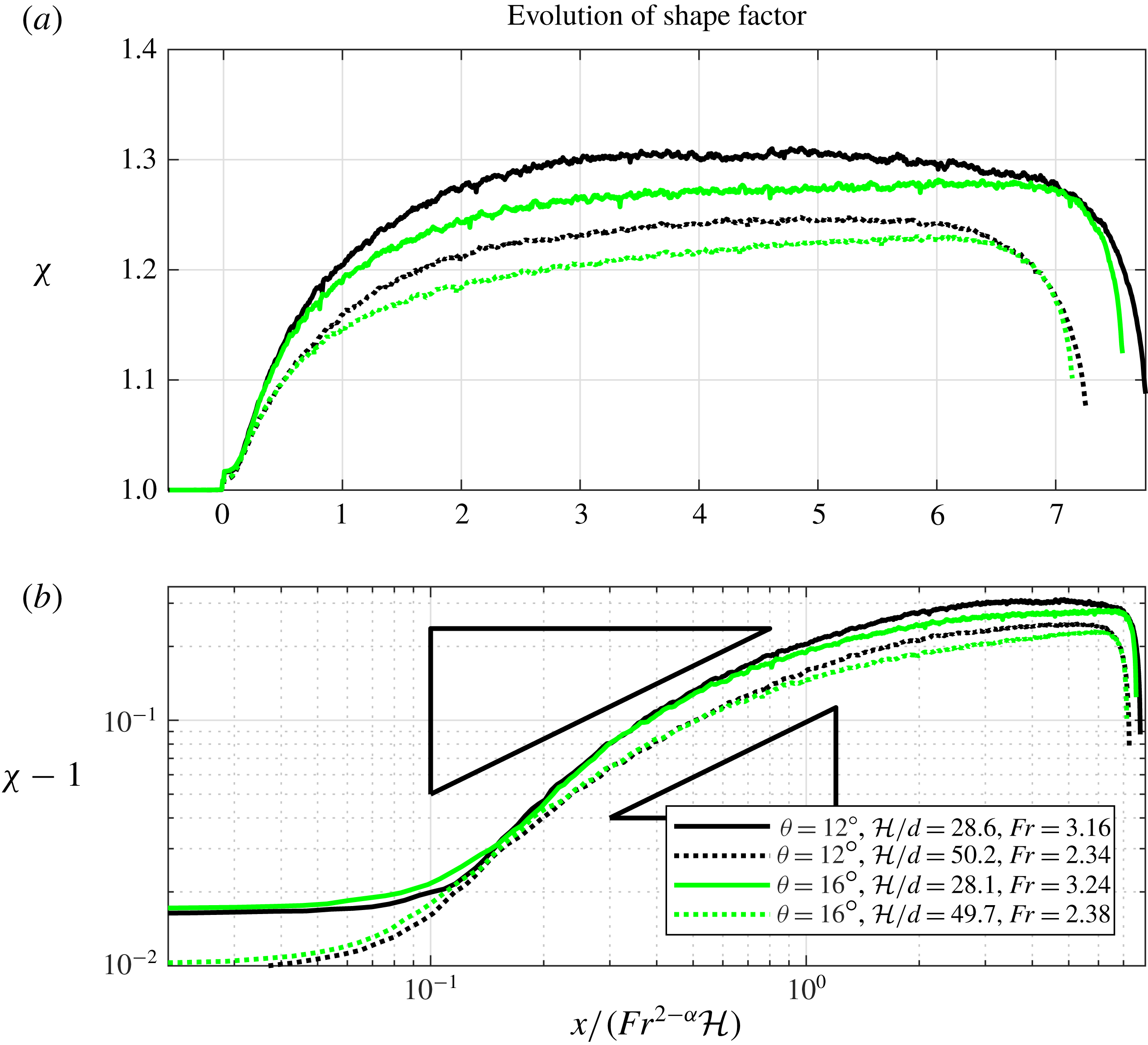
 ${\mathcal{U}}\approx 3$
. (a) Shape factor
 $\unicode[STIX]{x1D712}$
against
 $x/(Fr^{2-\unicode[STIX]{x1D6FC}}{\mathcal{H}})$
. (b) A log–log plot of
 $\unicode[STIX]{x1D712}-1$
against
 $x/(Fr^{2-\unicode[STIX]{x1D6FC}}{\mathcal{H}})$
for
 $x>0$
, with triangles indicating the power law predicted in (5.5).

We see from figure 6(b) that the slip velocity decays to almost zero for
 $x\approx 0.5Fr{\mathcal{H}}$
. The no-slip condition is not applicable just to the right of
 $x=0$
. This, together with the behaviour of
 $\unicode[STIX]{x1D719}$
discussed in § 5.1, suggests that the analysis of § 4 does not apply in
 $0\leqslant x<0.5Fr{\mathcal{H}}$
, but we expect the similarity solutions found in § 4.3 to hold for
 $0.5Fr{\mathcal{H}}\leqslant x\leqslant Fr^{2}{\mathcal{H}}$
.
5.3 Evolution of the velocity profile
We first discuss the velocity profiles in the boundary-layer region. While there is no definite cutoff between the boundary layer and the outer layer, for the sake of description we focus on the region
 $\unicode[STIX]{x1D701}/\unicode[STIX]{x1D701}_{disp}<2$
; this is reasonable because
 $2\unicode[STIX]{x1D701}_{disp}$
is approximately the 90th percentile of
 $f$
, as
 $f(2\unicode[STIX]{x1D701}_{disp})\approx 0.9$
. Figure 7 shows the velocity profiles from a set of eight DPM simulations in which
 $\unicode[STIX]{x1D703}$
and
 ${\mathcal{U}}$
were varied. In each panel of figure 7 we plot the scaled velocity
 $u/{\mathcal{U}}$
against the similarity variable
 $\unicode[STIX]{x1D701}/\unicode[STIX]{x1D701}_{disp}=z/(\unicode[STIX]{x1D701}_{disp}\unicode[STIX]{x1D6EC}(x))$
at different values of
 $x$
along the flow, where
 $\unicode[STIX]{x1D6EC}(x)$
is calculated from (4.18). We mark also the predicted similarity profile
 $f^{\prime }(\unicode[STIX]{x1D701})$
(continuous; black online) and the profiles at
 $x=0.5Fr{\mathcal{H}}$
(dot-dash; blue online) and at
 $x=Fr^{2}{\mathcal{H}}$
(dotted; blue online).
In most of the panels, the profiles at
 $x=0.5Fr{\mathcal{H}}$
and at
 $x=Fr^{2}{\mathcal{H}}$
collapse very well onto each other, indicating that the boundary-layer velocity profiles between these two positions exhibit the predicted self-similarity. Except for figures 7(a) and 7(e), which have the two lowest Froude numbers, the profiles near
 $x=0.5Fr{\mathcal{H}}$
also align well with the predicted similarity profile
 $f^{\prime }(\unicode[STIX]{x1D701})$
. Subsequent profiles begin to diverge from the black curve, especially after
 $x=Fr^{2}{\mathcal{H}}$
, as the boundary-layer thickness grows and becomes comparable with the depth of the current, interacting with the free surface. With the lower Froude numbers, the fit is less good: the assumption that
 $Fr\gg 1$
, made in § 4.3, does not apply very well.
In the outer layer
 $\unicode[STIX]{x1D701}/\unicode[STIX]{x1D701}_{disp}>2$
, the velocity is approximately uniform at the more upstream (darker curves; red online) positions, especially at higher Froude numbers, but this is less so at the more downstream (lighter curves; orange online) positions, where the division into a boundary layer and an outer layer becomes invalid. The velocity in the outer layer does not remain constant, but gradually increases. This is due to streamwise acceleration due to gravity, which is greater in figure 7(e–h) than in figure 7(a–d), due to the larger value of
 $\unicode[STIX]{x1D703}$
.
For the simulations presented in figure 7, we show also the evolution of the velocity profile in figure 8, in which we plot
 $u/\overline{u}$
against a scaled perpendicular coordinate
 $\unicode[STIX]{x1D702}=z/h(x)$
. In each panel, the current progresses towards a Bagnoldian profile (continuous black curve), but this is not reached by the position
 $x=Fr^{2}{\mathcal{H}}$
or even by
 $x=2.5Fr^{2}{\mathcal{H}}$
. This suggests that the decay of the incident inertia takes place over a longer length scale than the
 $O(Fr^{2}{\mathcal{H}})$
that would be predicted by depth-averaged models and our scaling arguments in § 4.1.
5.4 Evolution of the shape factor
As mentioned in § 1, each velocity profile may be characterised by the shape factor
 $\unicode[STIX]{x1D712}$
. The evolution of
 $\unicode[STIX]{x1D712}$
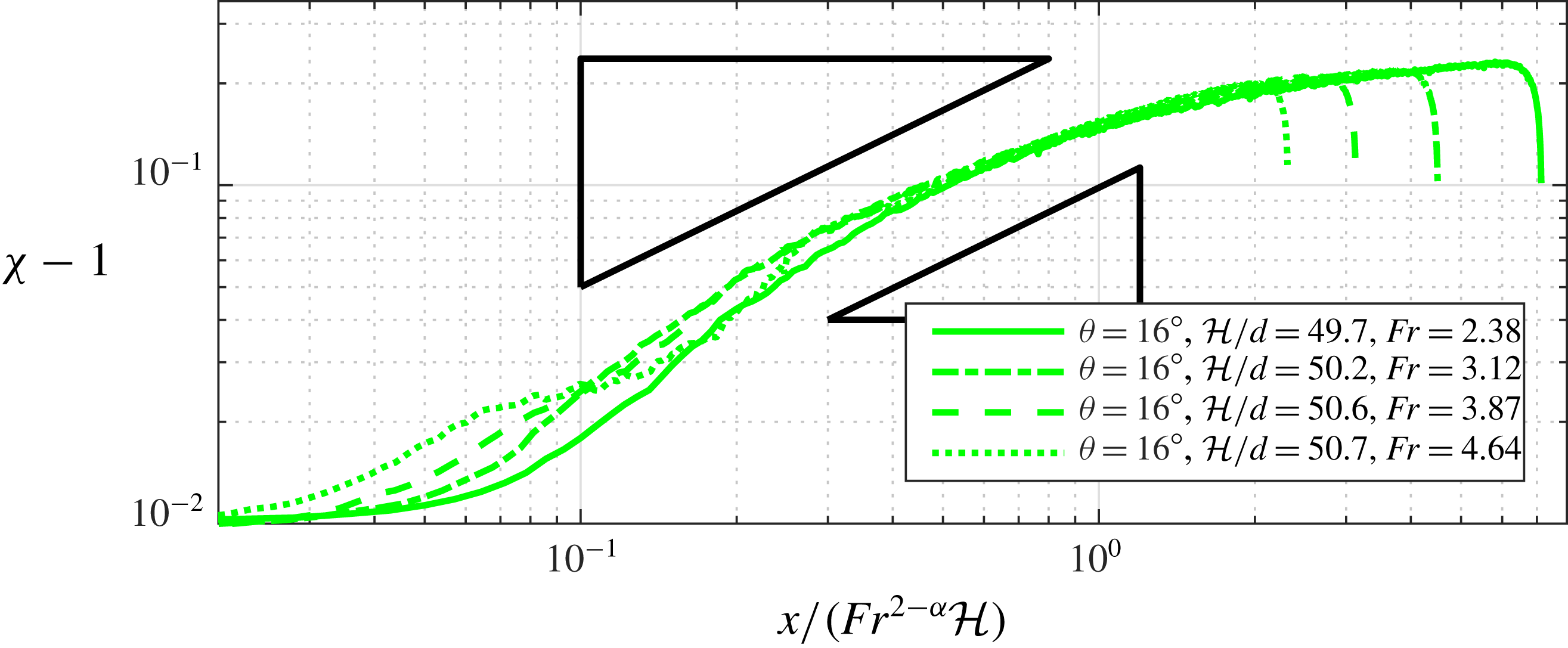
along the current in the various simulations is shown in figures 9 and 10.
The behaviours for a fixed value of
 ${\mathcal{U}}\approx 3$
and two settings for each of
 $\unicode[STIX]{x1D703}$
(colours) and
 ${\mathcal{H}}$
(line styles) are shown in figure 9(a). In each case, the incident current in
 $x<0$
has
 $\unicode[STIX]{x1D712}\approx 1$
, as expected. The same data are shown as a log–log plot of
 $\unicode[STIX]{x1D712}-1$
against
 $x/(Fr^{2}{\mathcal{H}})$
in figure 9(b), which allows a comparison against the predicted power-law growth for
 $\unicode[STIX]{x1D712}-1$
(4.31). For each setting of
 ${\mathcal{H}}$
, the two curves for that setting (with the same line style) collapse onto each other in the region
 $10^{-1}Fr^{2}{\mathcal{H}}<x<Fr^{2}H$
; moreover, all four curves are approximately parallel to each other.
In each of the four cases, the shape factors tend towards constants
 $\unicode[STIX]{x1D712}_{\infty }$
as
 $x\rightarrow \infty$
, indicating that velocity profiles become saturated. For the deeper currents (dotted lines),
 $\unicode[STIX]{x1D712}_{\infty }\approx 5/4$
, appropriate for a Bagnoldian profile: in these simulations, in which
 ${\mathcal{H}}/d\approx 50$
, the current is sufficiently deep that such a profile is adopted. For the shallower currents (solid lines),
 $\unicode[STIX]{x1D712}_{\infty }>5/4$
, indicating a profile other than the Bagnoldian one. This excess is due to the grain size being too large compared to the depth, and we discuss this issue further in § 6.3. The drops in
 $\unicode[STIX]{x1D712}$
near the end of each profile are an artefact from the deletion boundary at the end of the domain.
The evolution of the shape factor for
 $\unicode[STIX]{x1D703}=16^{\circ }$
and
 ${\mathcal{H}}/d\approx 50$
, and four different values of
 ${\mathcal{U}}$
, shown as a log–log plot of
 $\unicode[STIX]{x1D712}-1$
against
 $x/(Fr^{2-\unicode[STIX]{x1D6FC}}{\mathcal{H}})$
for
 $x>0$
. The triangles indicate the power law predicted in (5.5).


In figure 10, we compare the evolutions of
 $\unicode[STIX]{x1D712}$
for four different values of
 ${\mathcal{U}}$
and therefore
 $Fr$
, with
 $\unicode[STIX]{x1D703}=16^{\circ }$
fixed and
 ${\mathcal{H}}\approx 50d$
kept approximately constant. These correspond to figures 7(e–h) and 8(e–h).
Using the formula (4.13) for
 $\unicode[STIX]{x1D716}$
and noting that
 ${\mathcal{H}}$
and
 $d$
are fixed, (4.31) predicts that
 $$\begin{eqnarray}\unicode[STIX]{x1D712}-1\sim \text{const.}\times Fr^{(-2+\unicode[STIX]{x1D6FC})/(1+\unicode[STIX]{x1D6FC})}(x/{\mathcal{H}})^{1/(1+\unicode[STIX]{x1D6FC})},\end{eqnarray}$$
and so
 $$\begin{eqnarray}\displaystyle \log (\unicode[STIX]{x1D712}-1) & {\sim} & \displaystyle \frac{1}{1+\unicode[STIX]{x1D6FC}}\log (x/{\mathcal{H}})-\frac{2-\unicode[STIX]{x1D6FC}}{1+\unicode[STIX]{x1D6FC}}\log Fr+\text{const.}\end{eqnarray}$$
 $$\begin{eqnarray}\displaystyle & {\approx} & \displaystyle 0.75\log (x/(Fr^{1.66}{\mathcal{H}}))+\text{const.},\end{eqnarray}$$
when we set
 $\unicode[STIX]{x1D6FC}=0.34$
. Therefore, in figure 10 we use a log–log plot of
 $\unicode[STIX]{x1D712}-1$
against the rescaled streamwise coordinate
 $x/(Fr^{2-\unicode[STIX]{x1D6FC}}{\mathcal{H}})$
. We show also the slope that (5.5) predicts. The curves collapse reasonably well onto each other and match with (5.5). However, as in § 5.3, the lowest Froude number (with
 $Fr=2.38$
, continuous line, corresponding to figures 7
e and 8
e) does not agree as well, as the assumption that
 $Fr\gg 1$
is not sufficiently satisfied here.
6 Discussion
6.1 Applicability of the no-slip condition
We saw in § 5.2 that the basal topography’s transition from smooth to bumpy reduces and eventually eliminates the slip velocity of the current, but we also saw that the slip velocity does not immediately vanish when the incoming flow is sufficiently fast. Thus, the no-slip condition is an appropriate assumption for much of the bumpy region
 $x>0$
, but the two are not equivalent. This is unsurprising from a continuum standpoint, because the boundary conditions in § 3.2 lead to an ill-posedness around the origin
 $(x,z)=(0,0)$
. The sudden imposition of the no-slip condition would imply that
 $|\unicode[STIX]{x2202}u/\unicode[STIX]{x2202}z|=\infty$
at that point, which by incompressibility would imply a singular value for
 $w$
. The issue must be resolved by noting both that the flow is in fact slightly compressible and that ‘no slip’, in a continuum sense, is not synonymous with ‘bumpy base’.
In a continuum model of a granular flow, a no-slip condition is expressed simply as a boundary condition on the velocity field imposed on a surface; here, the boundary
 $z=0$
for
 $x>0$
. This condition does not come from first principles, and does not necessarily describe the motion of discrete grains against a wall, when flows are realised either in laboratory experiments or in DPM simulations. At the discrete level, an individual grain may be able to slide or roll along the wall. The problem is comparable to the no-slip condition for viscous fluids, which also does not follow from first principles but from observations of fluids. As noted by Acheson (Reference Acheson1990), early fluid dynamicists were hesitant to impose this condition for high-Reynolds-number flows. As an example, simulations by Morris, Hannon & Garcia (Reference Morris, Hannon and Garcia1992) suggest that a dilute viscous gas moving against a smooth wall exhibits a slip velocity
 $u_{s}$
which can be interpreted as
 $$\begin{eqnarray}u_{s}\propto \unicode[STIX]{x1D706}{\displaystyle \frac{\unicode[STIX]{x2202}u}{\unicode[STIX]{x2202}z}}\propto \frac{\unicode[STIX]{x1D706}\unicode[STIX]{x1D70E}_{xz}}{\unicode[STIX]{x1D702}},\end{eqnarray}$$
where
 $\unicode[STIX]{x1D706}$
is the mean free path of the gas molecules,
 $\unicode[STIX]{x2202}u/\unicode[STIX]{x2202}z$
is the velocity gradient at the wall,
 $\unicode[STIX]{x1D70E}_{xz}$
is the shear stress on the wall and here
 $\unicode[STIX]{x1D702}$
is the dynamic viscosity of the gas (Hui et al.
Reference Hui, Haff, Ungar and Jackson1984). The first proportionality in (6.1) was postulated by Maxwell (Reference Maxwell1879). The second proportionality comes from the Newtonian law
 $\unicode[STIX]{x1D70E}_{xz}/\unicode[STIX]{x1D702}\propto \unicode[STIX]{x2202}u/\unicode[STIX]{x2202}z$
, although ‘the viscosity [of a gas] in the Knudsen layer is lower in comparison with the viscosity in the bulk fluid’ (Fichman & Hetsroni Reference Fichman and Hetsroni2005), where the Knudsen layer is the region of thickness
 $\unicode[STIX]{x1D706}$
from the wall.
For a dense granular flow, whether or not the no-slip condition holds at a wall depends both on the geometric roughness of the wall and on the intrinsic friction between the wall and a grain moving against it. All materials have asperities, at the microscopic level, that provide a frictional resistance to sliding motions. In this article, by ‘roughness’ or ‘smoothness’ we refer to features on length scales comparable to the grain size, which give a geometrical constraint on the motion of grains.
The motion of a single circular grain moving against a geometrically smooth but frictional wall was considered through discrete simulations in Artoni, Santomaso & Canu (Reference Artoni, Santomaso and Canu2009). There, the grain was subject to random applied forces that represent the effect of all the other grains in the system. It was shown that the motion of the grain depends on whether the applied tangential force exceeds a certain threshold, which is proportional to the friction between the grain and the wall. It was shown that if the applied tangential force does not exceed this threshold, then the particle does not move at all; otherwise, the particle translates intermittently with a positive mean velocity, exhibiting a stick–slip behaviour.
The simulations of Morris et al. (Reference Morris, Hannon and Garcia1992) and Artoni et al. (Reference Artoni, Santomaso and Canu2009) considered only geometrically smooth walls. When the walls have geometric roughness of amplitude comparable to the grain size, this greatly reduces the mean free path of any grains moving against the wall. This effects a no-slip condition by confining grains from rolling or sliding along the surface. This may happen even if there is no intrinsic friction, as with the simulations described in this article.
Recent DPM simulations by Bharathraj & Kumaran (Reference Bharathraj and Kumaran2017) have shown that for currents flowing over frozen-particle bumpy bases, the no-slip condition applies if and only if the amplitude of the bumpiness exceeds a certain critical value. Jing et al. (Reference Jing, Kwok, Leung and Sobral2016) have proposed a non-dimensional parameter that quantifies the roughness of a frozen-particle base, in terms of the relative sizes of the diameters of the flowing and basal particles, and the density and geometric arrangement of the basal particles.
However, despite the large volume of work studying boundary conditions on granular flows using DPMs (Morris et al.
Reference Morris, Hannon and Garcia1992; Artoni et al.
Reference Artoni, Santomaso and Canu2009; Jing et al.
Reference Jing, Kwok, Leung and Sobral2016; Bharathraj & Kumaran Reference Bharathraj and Kumaran2017), it is unlikely that any continuum model will ever satisfactorily describe the decay of slip velocity immediate at a transition in basal topography, as seen in figure 6. We found that this decay depends sensitively on the precise nature of the transition, in preliminary simulations in which we did not use the mollified transition (5.1), but instead a step change in bumpiness (equivalent to substituting
 $\tanh (x_{n}/{\mathcal{M}})-1$
with
 $0$
in (5.1)).
6.2 Perturbation to the outer flow
In order to make progress in § 4.2, we assumed that the outer flow retains its incident velocity and pressure, with no streamwise pressure gradient. In reality, the streamwise deceleration in the boundary layer leads to a displacement velocity
 $w>0$
in the depthwise direction, which induces a perturbation to the outer flow, causing the outer flow to slow down and the free surface to be displaced upwards as
 $x$
increases. This is in contrast to the classical Blasius problem, in which the outer flow is imposed and its behaviour is not coupled to that of the boundary layer.
When analysing the boundary layer, neglecting the perturbation to the outer layer is appropriate only if this perturbation has a subdominant effect on the boundary layer. For a Newtonian current under a free surface with Reynolds number
 $Re$
and Froude number
 $Fr$
, the perturbation was calculated in Tsang et al. (Reference Tsang, Dalziel and Vriend2018), and was found to be small in the limit
 $Re\rightarrow \infty$
with
 $Fr$
fixed, but not if the Froude number is sufficiently close to 1. We have not shown that the same is true in the granular case, since we have not calculated the perturbation to the outer flow. Nonetheless, the boundary-layer self-similarity (4.15) implied by this assumption appears to match well with the results of DPM simulations at Froude numbers
 $Fr\geqslant 3.07$
(see figure 7). This is reasonable, since, informally, a high-Froude-number flow carries the ‘information’ from far upstream. Indeed, in both problems, the Froude number represents the speed of the characteristics (Evans Reference Evans2010) in the depth-averaged governing equations.
In the transitional region containing the boundary layer, the scaling laws (4.31) and (4.32) for the shape factor appear to be supported by the results of figures 9 and 10, even though they were obtained from simple arguments that did not require the computation of the perturbation to the outer flow. However, such a computation would give the constant of proportionality
 $c$
that appears in (4.32). This constant
 $c$
could be found by solving the system of equations that govern the perturbation to the outer flow, given in appendix C.
6.3 Alternative rheological models
The analysis above focused on the
 $\unicode[STIX]{x1D707}(I)$
rheology and straightforward generalisations, but this problem could be studied under different rheological models of dry granular flows. The granular boundary-layer equation (4.7) resembles the classical boundary-layer equation (4.9) on account of the second derivative
 $\unicode[STIX]{x2202}^{2}u/\unicode[STIX]{x2202}\tilde{z}^{2}$
in the final terms of both equations. This term appears in obtaining (4.7) from (3.7a
) because the shear stress term
 $\unicode[STIX]{x1D70E}_{xz}=\unicode[STIX]{x1D707}(I)pt_{xz}$
has a dependence on
 $\unicode[STIX]{x2202}u/\unicode[STIX]{x2202}z$
through the inertial number
 $I$
. We therefore expect a similar structure of equations in any rheology where the shear stress depends on the local strain rate. For such rheologies, it will be possible to perform boundary-layer analyses similar to that of § 4. Most rheological models are strain-rate-dependent, with a notable exception being the Mohr–Coulomb rheology (Andreotti et al.
Reference Andreotti, Forterre and Pouliquen2015), in which
 $\unicode[STIX]{x1D70E}_{xz}=\unicode[STIX]{x1D707}pt_{xz}$
for a constant coefficient of friction
 $\unicode[STIX]{x1D707}$
.
Under the
 $\unicode[STIX]{x1D707}(I)$
rheology, we assume that the grain size
 $d$
, or its non-dimensionalised value
 $\unicode[STIX]{x1D6FF}=d/{\mathcal{H}}$
, affects the system only through its appearance in the inertial number (3.5). While
 $\unicode[STIX]{x1D6FF}$
affects the boundary-layer thickness (4.25), it is treated merely as a material parameter. The
 $\unicode[STIX]{x1D707}(I)$
rheology is ‘local’, in the sense that the stress tensor at a point (3.3) depends only on the local values of the pressure and shear rate, and not on their derivatives. Perhaps unsurprisingly, experimental work has shown that this approach is unsatisfactory when there are gradients over distances comparable to
 $d$
(Kamrin & Henann Reference Kamrin and Henann2015). In particular, inclined chute flows stop if the depth
 $h$
falls below a certain value
 $h_{stop}(\unicode[STIX]{x1D703})=O(d)$
. In contrast, the
 $\unicode[STIX]{x1D707}(I)$
rheology gives excellent comparisons with experiments when
 $h\gg h_{stop}$
(or equivalently when
 $\unicode[STIX]{x1D6FF}\ll 1$
), but not when the flow is not sufficiently deep compared to the grain size. This has motivated the development of a number of ‘non-local’ constitutive relations, which modify the
 $\unicode[STIX]{x1D707}(I)$
rheology by allowing the stress tensor to depend on gradients of
 $I$
over length scales proportional to
 $d$
. Such models include the ‘cooperative model’ (Henann & Kamrin Reference Henann and Kamrin2013; Kamrin & Henann Reference Kamrin and Henann2015) and the ‘gradient model’ (Bouzid et al.
Reference Bouzid, Trulsson, Claudin, Clément and Andreotti2013).
Under the cooperative model, the stress tensor
 $\unicode[STIX]{x1D748}$
depends not only on
 $I$
, but also on
 $\unicode[STIX]{x1D6FB}^{2}I$
. Since
 $I$
in turn depends on velocity gradients,
 $\unicode[STIX]{x1D735}\boldsymbol{\cdot }\unicode[STIX]{x1D748}$
gives a term depending on
 $\unicode[STIX]{x1D6FB}^{4}\boldsymbol{u}$
in (3.1b
). This extra term represents non-local effects, and it could give rise to an ‘inner-inner layer’, that is, a second boundary layer with a thickness proportional to the grain size, in addition to the one that has been studied in this article.
The aforementioned models all concern dry granular flows where the medium between grains has no dynamical importance. For mixtures of particles in water, Longo & Valiani (Reference Longo and Valiani2014) have conducted an experimental study of a similar problem, involving a three-dimensional free-surface flow onto a blade that is aligned vertically and along the flow. As in the classical and granular Blasius problems, the blade in Longo & Valiani (Reference Longo and Valiani2014) imposes a no-slip condition that creates a boundary layer near the blade. These boundary layers are also self-similar, with a different profile from that of the classical Blasius boundary layer or those discussed in this paper, owing to the different rheological properties of the suspensions.
7 Conclusions
We have considered a steady granular current flowing down a slope. The basal condition is free slip in the upstream region
 $x<0$
but no slip for
 $x>0$
. This problem is a prototypical example of a small-scale topographical change affecting a granular current. The change in basal boundary condition creates a change in the internal velocity profile, which cannot be captured under a depth-averaged model.
The sudden imposition of a no-slip condition makes this problem analogous to the classical Blasius problem, but the Navier–Stokes equations of the classical problem are replaced by the
 $\unicode[STIX]{x1D707}(I)$
rheology for a granular material. The
 $\unicode[STIX]{x1D707}(I)$
rheology predicts that for a rapid incident flow, the velocity profile is asymptotically plug-like for
 $x\rightarrow -\infty$
and Bagnoldian for
 $x\rightarrow \infty$
. As in the classical Blasius problem, the no-slip condition for
 $x>0$
induces a distortion in the velocity profile, in a boundary layer initially localised near the base
 $z=0$
, but whose thickness grows along the streamwise direction.
We have used a Prandtl-like analysis of the
 $\unicode[STIX]{x1D707}(I)$
equations to study the development of the boundary layer in a transitional region
 $x\ll Fr^{2}{\mathcal{H}}$
. We showed that the boundary-layer thickness and velocity profile are determined by the asymptotic behaviour of
 $\unicode[STIX]{x1D707}(I)$
as
 $I\rightarrow \infty$
, and that the Jop fit (3.6) does not yield a valid boundary-layer scaling. However, certain alternative behaviours of the form (4.10) give self-similar solutions for the velocity profile in the boundary layer, and the scalings match well with results from two-dimensional DPM simulations.
While it would be interesting to conduct more realistic but computationally more costly DPM simulations in three dimensions, we have nevertheless shown that simple simulations in two dimensions with
 ${\mathcal{H}}/d\approx 50$
are sufficient to produce boundary layers that give a good agreement with theory. This agreement opens up the possibility of exploring more complex scenarios.
As we have shown in this work, there are various theoretical aspects of this problem that should be considered in the future. More accurate expressions for
 $\unicode[STIX]{x1D712}$
and
 $h(x)$
might be obtained by finding the perturbation to the outer flow induced by the boundary layer (§ 6.2). Alternative rheological models could give more accurate expressions when the grain size
 $d$
is not sufficiently small (§ 6.3), and the approach taken in the present work could be used to study boundary layers in other non-Newtonian fluids.
Acknowledgements
The DPM simulations were conducted using MercuryDPM (Thornton et al. Reference Thornton, Weinhart, Luding and Bokhove2012, Reference Thornton, Krijgsman, te Voortwis, Ogarko, Luding, Fransen, Gonzalez, Bokhove, Imole and Weinhart2013; Weinhart et al. Reference Weinhart, Thornton, Luding and Bokhove2012, Reference Weinhart, Tunuguntla, Lantman, van Schrojenstein, Windows-Yule, Polman, Tsang, Jin, Orefice and van der Vaart2017), an open source package developed at the University of Twente (http://www.mercurydpm.org). We thank A. Thornton, T. Weinhart, D. Tunuguntla, I. Denissen and B. Jin for their technical assistance with MercuryDPM. We also thank A. Thomas, M. Arran, P. Jarvis, S. Riber, S. Cowley and J. Hinch for discussions on this work. J.M.F.T. is funded by an EPSRC Studentship (EP/M508007/1) and N.M.V. is a Royal Society Dorothy Hodgkin Research Fellow (DH120121).
Appendix A. Derivation of the granular Blasius equation (4.7)
Here we derive (4.7) from (3.7a
) and (3.7b
). Under the scalings (4.5a
) for the boundary layer, the strain direction tensor
 $\unicode[STIX]{x1D668}$
is greatly simplified at leading order in
 $O(\unicode[STIX]{x1D716})$
, with
 $$\begin{eqnarray}\unicode[STIX]{x1D634}_{xx}=O(\unicode[STIX]{x1D716}),\quad \unicode[STIX]{x1D634}_{zz}=O(\unicode[STIX]{x1D716}),\quad \unicode[STIX]{x1D634}_{xz}=\unicode[STIX]{x1D634}_{zx}=1+O(\unicode[STIX]{x1D716}^{2}).\end{eqnarray}$$
From this we estimate the size of each term of (3.7b ):
 $$\begin{eqnarray}\displaystyle & \displaystyle \unicode[STIX]{x1D716}Fr^{2}\left(\tilde{u} {\displaystyle \frac{\unicode[STIX]{x2202}\tilde{w}}{\unicode[STIX]{x2202}\tilde{x}}}+\tilde{w}{\displaystyle \frac{\unicode[STIX]{x2202}\tilde{w}}{\unicode[STIX]{x2202}\tilde{z}}}\right)=-\cos \unicode[STIX]{x1D703}-\frac{1}{\unicode[STIX]{x1D716}}{\displaystyle \frac{\unicode[STIX]{x2202}\tilde{p}}{\unicode[STIX]{x2202}\tilde{z}}}+{\displaystyle \frac{\unicode[STIX]{x2202}(\unicode[STIX]{x1D707}(I)\tilde{p}\unicode[STIX]{x1D634}_{xz})}{\unicode[STIX]{x2202}\tilde{x}}}+{\displaystyle \frac{\unicode[STIX]{x2202}(\unicode[STIX]{x1D707}(I)\tilde{p}\unicode[STIX]{x1D634}_{zz})}{\unicode[STIX]{x2202}\tilde{z}}} & \displaystyle\end{eqnarray}$$
 $$\begin{eqnarray}\displaystyle & \displaystyle \Rightarrow \unicode[STIX]{x1D716}Fr^{2}\left(\tilde{u} {\displaystyle \frac{\unicode[STIX]{x2202}\tilde{w}}{\unicode[STIX]{x2202}\tilde{x}}}+\tilde{w}{\displaystyle \frac{\unicode[STIX]{x2202}\tilde{w}}{\unicode[STIX]{x2202}\tilde{z}}}\right)=-\frac{1}{\unicode[STIX]{x1D716}}{\displaystyle \frac{\unicode[STIX]{x2202}\tilde{p}}{\unicode[STIX]{x2202}\tilde{z}}}+O(1) & \displaystyle\end{eqnarray}$$
 $$\begin{eqnarray}\displaystyle & \displaystyle \Rightarrow O(\unicode[STIX]{x1D716}^{2}Fr^{2})=-{\displaystyle \frac{\unicode[STIX]{x2202}p}{\unicode[STIX]{x2202}\tilde{z}}}+O(\unicode[STIX]{x1D716}). & \displaystyle\end{eqnarray}$$
We postulate
 $\unicode[STIX]{x1D716}Fr\ll 1$
, but must later confirm the validity of this assertion (see § 4.3 and appendix B). The assumption
 $Fr\gg 1$
therefore requires
 $\unicode[STIX]{x1D716}\ll 1$
. Then according to (A 4),
 $|\unicode[STIX]{x2202}\tilde{p}/\unicode[STIX]{x2202}\tilde{z}|$
is small in the boundary layer, so that the pressure across the boundary layer is given by the pressure from the outer flow, which is the lithostatic pressure
 $\tilde{p}=\tilde{h}\cos \unicode[STIX]{x1D703}$
. If the depth
 $h$
is taken to be locally constant (as discussed in the main text), then
 $\unicode[STIX]{x2202}\tilde{p}/\unicode[STIX]{x2202}\tilde{x}$
vanishes as well, so that, to leading order,
 $p$
is constant throughout the boundary layer. By definition, the depth of the incident flow is
 ${\mathcal{H}}$
, so
 $\tilde{h}=1$
and we write
 $\tilde{p}=\cos \unicode[STIX]{x1D703}$
.
We now consider (3.7a ). When the rescalings (4.5a ) are applied, (3.7a ) becomes
 $$\begin{eqnarray}\displaystyle Fr^{2}\left(\tilde{u} {\displaystyle \frac{\unicode[STIX]{x2202}\tilde{u} }{\unicode[STIX]{x2202}\tilde{x}}}+\tilde{w}{\displaystyle \frac{\unicode[STIX]{x2202}\tilde{u} }{\unicode[STIX]{x2202}\tilde{z}}}\right) & = & \displaystyle \sin \unicode[STIX]{x1D703}+\frac{1}{\unicode[STIX]{x1D716}}{\displaystyle \frac{\unicode[STIX]{x2202}(\unicode[STIX]{x1D707}(I)\tilde{p})}{\unicode[STIX]{x2202}\tilde{z}}}+O(\unicode[STIX]{x1D716})\end{eqnarray}$$
 $$\begin{eqnarray}\displaystyle & = & \displaystyle \sin \unicode[STIX]{x1D703}+\frac{1}{\unicode[STIX]{x1D716}}\unicode[STIX]{x1D707}(I){\displaystyle \frac{\unicode[STIX]{x2202}\tilde{p}}{\unicode[STIX]{x2202}\tilde{z}}}+\frac{1}{\unicode[STIX]{x1D716}}\tilde{p}{\displaystyle \frac{\text{d}\unicode[STIX]{x1D707}}{\text{d}I}}{\displaystyle \frac{\unicode[STIX]{x2202}I}{\unicode[STIX]{x2202}\tilde{z}}},\end{eqnarray}$$
the other terms being subdominant. To proceed, we calculate the inertial number. To leading order, the magnitude of the shear rate tensor is
 $$\begin{eqnarray}\Vert \tilde{\unicode[STIX]{x1D63F}}\Vert =\frac{1}{2\unicode[STIX]{x1D716}}{\displaystyle \frac{\unicode[STIX]{x2202}\tilde{u} }{\unicode[STIX]{x2202}\tilde{z}}}+O(\unicode[STIX]{x1D716}),\end{eqnarray}$$
so the inertial number (3.5) is
 $$\begin{eqnarray}I\sim \frac{\unicode[STIX]{x1D6FF}Fr}{\unicode[STIX]{x1D716}\tilde{p}^{1/2}}{\displaystyle \frac{\unicode[STIX]{x2202}\tilde{u} }{\unicode[STIX]{x2202}\tilde{z}}},\end{eqnarray}$$
and
 $$\begin{eqnarray}\frac{1}{I}{\displaystyle \frac{\unicode[STIX]{x2202}I}{\unicode[STIX]{x2202}\tilde{z}}}\sim -\frac{1}{2\tilde{p}}{\displaystyle \frac{\unicode[STIX]{x2202}\tilde{p}}{\unicode[STIX]{x2202}\tilde{z}}}+\frac{\unicode[STIX]{x2202}^{2}\tilde{u} /\unicode[STIX]{x2202}\tilde{z}^{2}}{\unicode[STIX]{x2202}\tilde{u} /\unicode[STIX]{x2202}\tilde{z}}.\end{eqnarray}$$
Expanding the derivative on the right-hand side of (A 5) yields
 $$\begin{eqnarray}\displaystyle Fr^{2}\left(\tilde{u} {\displaystyle \frac{\unicode[STIX]{x2202}\tilde{u} }{\unicode[STIX]{x2202}\tilde{x}}}+\tilde{w}{\displaystyle \frac{\unicode[STIX]{x2202}\tilde{u} }{\unicode[STIX]{x2202}\tilde{z}}}\right) & {\sim} & \displaystyle \sin \unicode[STIX]{x1D703}+\frac{1}{\unicode[STIX]{x1D716}}{\displaystyle \frac{\unicode[STIX]{x2202}\tilde{p}}{\unicode[STIX]{x2202}\tilde{z}}}\left(\unicode[STIX]{x1D707}-\frac{1}{2}{\displaystyle \frac{\text{d}\unicode[STIX]{x1D707}}{\text{d}I}}I\right)\nonumber\\ \displaystyle & & \displaystyle +\,\frac{1}{\unicode[STIX]{x1D716}}\tilde{p}{\displaystyle \frac{\text{d}\unicode[STIX]{x1D707}}{\text{d}I}}I\frac{\unicode[STIX]{x2202}^{2}\tilde{u} /\unicode[STIX]{x2202}\tilde{z}^{2}}{\unicode[STIX]{x2202}\tilde{u} /\unicode[STIX]{x2202}\tilde{z}},\end{eqnarray}$$
which is (4.7), as required.
Appendix B. Conditions under which
$\unicode[STIX]{x1D716}Fr\ll 1$

The derivation of (4.7), given in appendix A, is valid only if the boundary-layer thickness scale
 $\unicode[STIX]{x1D716}$
satisfies
 $\unicode[STIX]{x1D716}Fr\ll 1$
, which was to be checked a posteriori.
The boundary-layer thickness scale for
 $\unicode[STIX]{x1D716}$
was given in (4.13). When it is stripped of
 $O(1)$
constants, we have
 $$\begin{eqnarray}\unicode[STIX]{x1D716}\propto (\unicode[STIX]{x1D6FF}^{\unicode[STIX]{x1D6FC}}Fr^{-(2-\unicode[STIX]{x1D6FC})})^{1/(1+\unicode[STIX]{x1D6FC})},\end{eqnarray}$$
and so
 $$\begin{eqnarray}\unicode[STIX]{x1D716}Fr\propto (\unicode[STIX]{x1D6FF}^{\unicode[STIX]{x1D6FC}}Fr^{2\unicode[STIX]{x1D6FC}-1})^{1/(1+\unicode[STIX]{x1D6FC})}.\end{eqnarray}$$
Assuming that
 $\unicode[STIX]{x1D6FC}>0$
, the required condition for
 $\unicode[STIX]{x1D716}Fr\ll 1$
is that
 $$\begin{eqnarray}\unicode[STIX]{x1D6FF}^{\unicode[STIX]{x1D6FC}}Fr^{2\unicode[STIX]{x1D6FC}-1}\ll 1.\end{eqnarray}$$
We note first that (B 3) is satisfied automatically if
 $\unicode[STIX]{x1D6FC}=0$
or
 $\unicode[STIX]{x1D6FC}=1/2$
, provided that
 $\unicode[STIX]{x1D6FF}\ll 1$
and
 $Fr\geqslant 1$
. For intermediate values
 $0<\unicode[STIX]{x1D6FC}<1/2$
, (B 3) becomes
 $$\begin{eqnarray}Fr\gg \unicode[STIX]{x1D6FF}^{\unicode[STIX]{x1D6FC}/(1-2\unicode[STIX]{x1D6FC})},\end{eqnarray}$$
which is automatically satisfied provided that
 $\unicode[STIX]{x1D6FF}\ll 1$
, as we insist that
 $Fr>1$
.
If instead
 $\unicode[STIX]{x1D6FC}>1/2$
, (B 3) becomes
 $$\begin{eqnarray}Fr\ll \unicode[STIX]{x1D6FF}^{-\unicode[STIX]{x1D6FC}/(2\unicode[STIX]{x1D6FC}-1)}.\end{eqnarray}$$
Our analysis is invalid if
 $Fr$
is large enough to violate (B 5), but since
 $\unicode[STIX]{x1D6FF}\ll 1$
the upper bound is large and the above condition is almost always satisfied in practice. For example, for
 $\unicode[STIX]{x1D6FC}=1$
, we have
 $\unicode[STIX]{x1D6FC}/(2\unicode[STIX]{x1D6FC}-1)1$
, and if
 $\unicode[STIX]{x1D6FF}=1/30$
then (B 5) holds up until
 $Fr\approx 30$
.
We also consider the cases
 $\unicode[STIX]{x1D6FC}<0$
. For
 $-1<\unicode[STIX]{x1D6FC}<0$
, (B 2) implies that
 $$\begin{eqnarray}Fr\gg \unicode[STIX]{x1D6FF}^{\unicode[STIX]{x1D6FC}/(1-2\unicode[STIX]{x1D6FC})}.\end{eqnarray}$$
This imposes a large lower bound on
 $Fr$
. On the other hand, for
 $\unicode[STIX]{x1D6FC}<-1$
, (B 2) is equivalent to
 $$\begin{eqnarray}Fr\ll \unicode[STIX]{x1D6FF}^{\unicode[STIX]{x1D6FC}/(1-2\unicode[STIX]{x1D6FC})},\end{eqnarray}$$
which, like (B 3), imposes an upper bound on
 $Fr$
. Note, however, that the case
 $\unicode[STIX]{x1D6FC}<-1$
predicts an incorrect behaviour for the boundary layer (see § 4.5). Finally, the case
 $\unicode[STIX]{x1D6FC}=-1$
is singular, owing to the power
 $1/(1+\unicode[STIX]{x1D6FC})$
in (B 2): the inequalities (B 6) and (B 7) have opposite signs.
To summarise, the condition
 $\unicode[STIX]{x1D716}Fr\ll 1$
is automatically satisfied for
 $0\leqslant \unicode[STIX]{x1D6FC}\leqslant 1/2$
. For realistic values of
 $\unicode[STIX]{x1D6FF}$
, the condition is usually satisfied for
 $\unicode[STIX]{x1D6FC}<-1$
or
 $\unicode[STIX]{x1D6FC}>1/2$
, and not satisfied for
 $-1<\unicode[STIX]{x1D6FC}<0$
.
Appendix C. Equations governing the perturbation to the outer flow
For simplicity, we work in non-dimensional units, scaling velocity components
 $u$
and
 $w$
by
 ${\mathcal{U}}$
, coordinates
 $x$
,
 $z$
and
 $h$
by
 ${\mathcal{H}}$
and pressure
 $p$
by
 $\unicode[STIX]{x1D70C}g{\mathcal{H}}$
, and drop tildes. To leading order in
 $\unicode[STIX]{x1D716}$
, let the outer flow velocity, pressure and depth be
 $$\begin{eqnarray}\left.\begin{array}{@{}c@{}}u=u^{(0)}(z)+\unicode[STIX]{x1D716}u^{(1)},\quad w=\unicode[STIX]{x1D716}w^{(1)},\\ p=p^{(0)}(z)+\unicode[STIX]{x1D716}p^{(1)},\quad h=1+\unicode[STIX]{x1D716}h^{(1)},\end{array}\right\}\end{eqnarray}$$
where
 $p^{(0)}(z)=\cos \unicode[STIX]{x1D703}({\mathcal{H}}-z)$
is the lithostatic pressure and
 $u^{(0)}(z)$
is the Bagnold-with-slip profile (4.1) of the incident flow. The shear rate tensor has magnitude
 $$\begin{eqnarray}\Vert \unicode[STIX]{x1D63F}\Vert =\frac{1}{2}{\displaystyle \frac{\text{d}u^{(0)}}{\text{d}z}}+\frac{1}{2}\unicode[STIX]{x1D716}\left[{\displaystyle \frac{\unicode[STIX]{x2202}u^{(1)}}{\unicode[STIX]{x2202}z}}+{\displaystyle \frac{\unicode[STIX]{x2202}w^{(1)}}{\unicode[STIX]{x2202}x}}\right],\end{eqnarray}$$
the shear direction tensor is
 $$\begin{eqnarray}\unicode[STIX]{x1D668}=\left[\begin{array}{@{}cc@{}}\displaystyle 2\unicode[STIX]{x1D716}\frac{\unicode[STIX]{x2202}u^{(1)}/\unicode[STIX]{x2202}x}{\text{d}u^{(0)}/\text{d}z} & 1\\ 1 & \displaystyle 2\unicode[STIX]{x1D716}\frac{\unicode[STIX]{x2202}w^{(1)}/\unicode[STIX]{x2202}z}{\text{d}u^{(0)}/\text{d}z}\end{array}\right],\end{eqnarray}$$
the inertial number is given by
 $$\begin{eqnarray}\displaystyle \frac{I}{\unicode[STIX]{x1D6FF}Fr} & = & \displaystyle \left((p^{(0)})^{-1/2}-\frac{1}{2}\unicode[STIX]{x1D716}(p^{(0)})^{-3/2}p^{(1)}\right)\left({\displaystyle \frac{\text{d}u^{(0)}}{\text{d}z}}+\frac{1}{2}\unicode[STIX]{x1D716}\left[{\displaystyle \frac{\unicode[STIX]{x2202}u^{(1)}}{\unicode[STIX]{x2202}z}}+{\displaystyle \frac{\unicode[STIX]{x2202}w^{(1)}}{\unicode[STIX]{x2202}x}}\right]\right)\end{eqnarray}$$
 $$\begin{eqnarray}\displaystyle & = & \displaystyle (p^{(0)})^{-1/2}{\displaystyle \frac{\text{d}u^{(0)}}{\text{d}z}}\end{eqnarray}$$
 $$\begin{eqnarray}\displaystyle & & \displaystyle +\,\unicode[STIX]{x1D716}\left[(p^{(0)})^{-1/2}\left[{\displaystyle \frac{\unicode[STIX]{x2202}u^{(1)}}{\unicode[STIX]{x2202}z}}+{\displaystyle \frac{\unicode[STIX]{x2202}w^{(1)}}{\unicode[STIX]{x2202}x}}\right]-\frac{1}{2}(p^{(0)})^{-3/2}{\displaystyle \frac{\text{d}u^{(0)}}{\text{d}z}}p^{(1)}\right]\end{eqnarray}$$
 $$\begin{eqnarray}\displaystyle & = & \displaystyle \frac{1}{\unicode[STIX]{x1D6FF}Fr}(I^{(0)}+\unicode[STIX]{x1D716}I^{(1)})\end{eqnarray}$$
and the friction coefficient is
 $$\begin{eqnarray}\displaystyle \unicode[STIX]{x1D707}(I) & = & \displaystyle \unicode[STIX]{x1D707}(I^{(0)})+\unicode[STIX]{x1D716}\unicode[STIX]{x1D707}^{\prime }(I^{(0)})I^{(1)}\end{eqnarray}$$
 $$\begin{eqnarray}\displaystyle & = & \displaystyle \tan \unicode[STIX]{x1D703}+\unicode[STIX]{x1D716}\unicode[STIX]{x1D707}^{\prime }(I^{(0)})I^{(1)},\end{eqnarray}$$
all up to
 $o(\unicode[STIX]{x1D716})$
error terms.
The equations governing the perturbation variables are the linearised momentum equations
 $$\begin{eqnarray}\displaystyle u^{(0)}{\displaystyle \frac{\unicode[STIX]{x2202}u^{(1)}}{\unicode[STIX]{x2202}x}}+{\displaystyle \frac{\text{d}u^{(0)}}{\text{d}z}}w^{(1)} & = & \displaystyle -{\displaystyle \frac{\unicode[STIX]{x2202}p^{(1)}}{\unicode[STIX]{x2202}x}}+\tan \unicode[STIX]{x1D703}{\displaystyle \frac{\unicode[STIX]{x2202}p^{(1)}}{\unicode[STIX]{x2202}z}}\nonumber\\ \displaystyle & & \displaystyle +\,{\displaystyle \frac{\unicode[STIX]{x2202}}{\unicode[STIX]{x2202}z}}(\unicode[STIX]{x1D707}^{\prime }(I^{(0)})p^{(0)}I^{(1)})\nonumber\\ \displaystyle & & \displaystyle +\,2p^{(0)}\tan \unicode[STIX]{x1D703}\frac{\unicode[STIX]{x2202}^{2}u^{(1)}/\unicode[STIX]{x2202}x^{2}}{\text{d}u^{(0)}/\text{d}z},\end{eqnarray}$$
 $$\begin{eqnarray}\displaystyle u^{(0)}{\displaystyle \frac{\unicode[STIX]{x2202}w^{(1)}}{\unicode[STIX]{x2202}x}} & = & \displaystyle -{\displaystyle \frac{\unicode[STIX]{x2202}p^{(1)}}{\unicode[STIX]{x2202}z}}+\tan \unicode[STIX]{x1D703}{\displaystyle \frac{\unicode[STIX]{x2202}p^{(1)}}{\unicode[STIX]{x2202}x}}\nonumber\\ \displaystyle & & \displaystyle +\,\unicode[STIX]{x1D707}^{\prime }(I^{(0)})p^{(0)}{\displaystyle \frac{\unicode[STIX]{x2202}I^{(1)}}{\unicode[STIX]{x2202}x}}+2{\displaystyle \frac{\unicode[STIX]{x2202}}{\unicode[STIX]{x2202}z}}\left(\frac{\unicode[STIX]{x2202}w^{(1)}/\unicode[STIX]{x2202}z}{\text{d}u^{(0)}/\text{d}z}\right),\end{eqnarray}$$
together with the incompressibility condition
 $$\begin{eqnarray}{\displaystyle \frac{\unicode[STIX]{x2202}u^{(1)}}{\unicode[STIX]{x2202}x}}+{\displaystyle \frac{\unicode[STIX]{x2202}w^{(1)}}{\unicode[STIX]{x2202}z}}=0.\end{eqnarray}$$
The linearised boundary conditions at the free surface are that
 $$\begin{eqnarray}w^{(1)}={\displaystyle \frac{\unicode[STIX]{x2202}h^{(1)}}{\unicode[STIX]{x2202}x}},\quad {\displaystyle \frac{\unicode[STIX]{x2202}u^{(1)}}{\unicode[STIX]{x2202}z}}=-{\displaystyle \frac{\unicode[STIX]{x2202}w^{(1)}}{\unicode[STIX]{x2202}x}}\quad \text{and}\quad p^{(1)}=h^{(1)}\cos \unicode[STIX]{x1D703}\quad \text{at }z=1,\end{eqnarray}$$
and the basal boundary condition on the perturbation flow is that
 $$\begin{eqnarray}w^{(1)}=w_{disp}(x)=\unicode[STIX]{x1D701}_{disp}u^{(0)}(0)\unicode[STIX]{x1D6EC}^{\prime }(x),\quad \text{at }z=0,\end{eqnarray}$$
where
 $w_{disp}(x)$
is the displacement velocity due to the boundary layer.
Although the system (C 10) and (C 11) is semilinear in the perturbation variables, no further analytical progress is possible, unlike the linear equations that arise for a Newtonian fluid as given in Tsang et al. (Reference Tsang, Dalziel and Vriend2018).


Appendix D. Density and temperature profiles
Figure 11 shows the profile of the packing fraction
 $\unicode[STIX]{x1D719}$
for the simulations presented in figures 7 and 8. Figure 12 shows the profile of the granular temperature, defined as the trace
 $T=\operatorname{tr}\unicode[STIX]{x1D64D}$
of the Reynolds stress tensor (Hinze Reference Hinze1975)
 $$\begin{eqnarray}\unicode[STIX]{x1D64D}=\langle \unicode[STIX]{x1D719}\boldsymbol{u}\boldsymbol{u}\rangle -\frac{\langle \unicode[STIX]{x1D719}\boldsymbol{u}\rangle \langle \unicode[STIX]{x1D719}\boldsymbol{u}\rangle }{\langle \unicode[STIX]{x1D719}\rangle },\end{eqnarray}$$
where angle brackets
 $$\begin{eqnarray}\langle f\rangle =\frac{1}{t_{2}-t_{1}}\int _{t_{1}}^{t_{2}}f(t)\,\text{d}t\end{eqnarray}$$
denote the time-average of a function
 $f$
. The plots in figure 12 are normalised by
 $T_{0}=\operatorname{trace}\unicode[STIX]{x1D64D}_{0}$
, where
 $$\begin{eqnarray}\unicode[STIX]{x1D64D}_{0}=\frac{\langle \unicode[STIX]{x1D719}\boldsymbol{u}\rangle \langle \unicode[STIX]{x1D719}\boldsymbol{u}\rangle }{\langle \unicode[STIX]{x1D719}\rangle }.\end{eqnarray}$$