1 Introduction
Internal waves are ubiquitous in Earth’s oceans, and a broad spectrum of frequencies and wavenumbers is observed (Garrett & Munk Reference Garrett and Munk1979; Holloway Reference Holloway1980; Garrett Reference Garrett2003). Most of their power, approximately 1 Terawatt globally, is found in low-frequency, low-mode baroclinic internal tides (Munk & Wunsch Reference Munk and Wunsch1998). These are observed globally, with a total energy content of the order of 36 Petajoules (global mean energy per unit mass
 $10^{-4}~\text{m}^{2}~\text{s}^{-2}$
) in the
 $M_{2}$
mode-1 component (Zhao et al.
Reference Zhao, Alford, Girton, Rainville and Simmons2016).
Dissipation of low-mode internal tides contributes substantially to ocean mixing (Garrett & Kunze Reference Garrett and Kunze2007). The geographic and vertical distribution of this dissipation has a significant impact on the mixing and thermal structure of the ocean, and incomplete understanding of dissipation contributes to errors in climate prediction (Melet et al. Reference Melet, Hallberg, Legg and Polzin2013). Multiple mechanisms have been proposed to explain the dissipation of the internal tides. Among these are scattering to smaller-scale internal waves by topography (Johnston & Merryfield Reference Johnston and Merryfield2003; Balmforth & Peacock Reference Balmforth and Peacock2009), interaction with mesoscale flow structures (Rainville & Pinkel Reference Rainville and Pinkel2006), shoaling on sloping continental shelves (Kunze & Llewellyn-Smith Reference Kunze and Llewellyn-Smith2004) and the parametric subharmonic instability (MacKinnon & Winters Reference MacKinnon and Winters2005; Xie et al. Reference Xie, Chen, Shang and Fang2008). It is plausible that no single dissipation mechanism is globally dominant, but instead that the relative importance of different mechanisms varies geographically and seasonally.
There has been much recent progress in understanding the nonlinear mechanisms which transfer internal wave energy to smaller scales, especially in the context of internal wave beams. One prominent example is the excitation of harmonics during beam reflection from walls (Tabaei & Akylas Reference Tabaei and Akylas2003; Peacock & Tabaei Reference Peacock and Tabaei2005; Tabaei, Akylas & Lamb Reference Tabaei, Akylas and Lamb2005; Rodenborn et al. Reference Rodenborn, Keifer, Zhang and Swinney2011) and mixed layers (Zhou & Diamessis Reference Zhou and Diamessis2013). Colliding beams also generate sum and difference harmonics, as has been shown theoretically by Tabaei et al. (Reference Tabaei, Akylas and Lamb2005), in the laboratory by Smith & Crockett (Reference Smith and Crockett2014) and in simulations by Lamb (Reference Lamb2004). Sufficiently wide internal wave beams are subject to nonlinear parametric subharmonic instability, leading to the formation of two subharmonic waves (Bourget et al. Reference Bourget, Dauxois, Joubaud and Odier2013; Gayen & Sarkar Reference Gayen and Sarkar2013). All of these mechanisms are due to interactions between waves of different frequencies or wavenumbers, and have usually been investigated using constant stratification.
An alternate possibility, which does not rely on wave–wave interactions, is the excitation of double-frequency and -wavenumber harmonics by a single mode in variable stratification. This harmonic effect was first observed for internal wave beams refracting through sharply increasing stratification by Grisouard and co-authors (Grisouard & Staquet Reference Grisouard and Staquet2010; Grisouard, Staquet & Gerkema Reference Grisouard, Staquet and Gerkema2011) using numerical simulations, and quickly followed in the laboratory by Mercier et al. (Reference Mercier, Mathur, Gostiaux, Gerkema, Magalhaes, da Silva and Dauxois2012) and Wunsch & Brandt (Reference Wunsch and Brandt2012). Additional numerical studies also observed the effect (Dossmann, Auclair & Paci Reference Dossmann, Auclair and Paci2013; Gayen & Sarkar Reference Gayen and Sarkar2013). Although the connection between harmonics and variable stratification was not recognized in these works, the subsequent weakly nonlinear theory of Diamessis et al. (Reference Diamessis, Wunsch, Delwiche and Richter2014) clearly derived the connection between variable stratification and harmonic generation by a single mode. This approach generalized the previous theoretical work of Thorpe (Reference Thorpe1998) and McHugh (Reference McHugh2009) showing harmonic generation for a plane wave in a two-layer fluid. For beams, the relative importance of this single-mode variable stratification effect compared to wave–wave interactions (which can occur in uniform stratification and generally give rise to double-frequency but not double-wavenumber harmonics) was further investigated by Wunsch et al. (Reference Wunsch, Ku, Delwiche and Awadallah2014, Reference Wunsch, Delwiche, Frederick and Brandt2015).
Mathematically, it is straightforward to transfer previous theoretical results for nonlinear refraction of a plane wave to single-mode internal tide self-interaction, as shown by Wunsch (Reference Wunsch2015). The first focused numerical study of single-mode internal waves (as opposed to beams) in variable stratification has recently been performed by Sutherland (Reference Sutherland2016). This work demonstrated the initial transient modes generated by nonlinear self-interaction in variable stratification, which have double the wavenumber of the forcing mode but are a superposition of different frequency modes. As the initial transients decayed, the dynamics progressed towards a bound double-frequency harmonic, and higher-order harmonics were also present. Feedback from the harmonic on the initial mode was also shown, suggesting that a significant harmonic effect might lead to the dissipation of the internal tide.
Double-frequency harmonics of oceanic internal tides were also observed in the South China Sea by Xie et al. (Reference Xie, Shang, van Haren and Chen2013), who immediately recognized the connection to the laboratory observations of Mercier et al. (Reference Mercier, Mathur, Gostiaux, Gerkema, Magalhaes, da Silva and Dauxois2012). The harmonic mode is transient, appearing and disappearing from the observed currents over periods of several days. The subsequent calculation of the expected steady-state bound harmonic amplitude by Wunsch (Reference Wunsch2015), using the weakly nonlinear theory of Diamessis et al. (Reference Diamessis, Wunsch, Delwiche and Richter2014), demonstrated that variable stratification was plausibly the cause of the observed harmonic. The bound harmonic amplitude depends strongly on the pycnocline characteristics, suggesting that gradual changes in the stratification profile might be responsible for the transient nature of the observations. Double-frequency harmonics have also been observed in numerical simulations of internal tides by Johnston & Merryfield (Reference Johnston and Merryfield2003), who noted that the harmonics only occurred when variable stratification was used.
Previous studies have not yet addressed the potential relevance of nonlinear self-interaction to ocean tidal dynamics and dissipation. Here, weakly nonlinear theory is used to explore the possible implications of nonlinear self-interaction for low-mode internal tides in the ocean. It is shown quite generally that the dynamics is analogous to a forced harmonic oscillator, and that a significant nonlinear response is possible even for weak forcing (i.e. a nearly linear wave) if the forcing frequency is comparable to a natural frequency of the system. The possibility of this near-resonant nonlinear self-interaction in the ocean is explored using an idealized stratification profile. In equatorial waters (no rotation), near-resonant conditions appear possible, which could lead to significant dissipation of the primary mode, as suggested by the simulations of Sutherland (Reference Sutherland2016). Elsewhere, resonance appears unlikely, so harmonics remain small compared to the primary mode and may not significantly alter the dynamics. Near resonance, the harmonic amplitude does not remain small and a full solution is beyond the scope of this approach. The present work demonstrates the value of weakly nonlinear analysis to identify near-resonant conditions, which would then require further study using numerical simulations, laboratory experiments or ocean observations.
2 Weakly nonlinear theory
Here, the second-order weakly nonlinear theory of single-mode internal wave self-interaction developed in Diamessis et al. (Reference Diamessis, Wunsch, Delwiche and Richter2014), Wunsch (Reference Wunsch2015) and Wunsch et al. (Reference Wunsch, Delwiche, Frederick and Brandt2015) for steady-state harmonics is extended to include transients, rotation and dissipation. Solutions are constructed by assuming a primary mode with wavenumber
 $k$
and frequency
 $\unicode[STIX]{x1D714}_{o}$
and then adding the perturbation generated by the nonlinear self-interaction of this mode. The perturbation dynamics is analogous to a forced harmonic oscillator and the solution consists of a steady-state bound harmonic (wavenumber
 $2k$
and frequency
 $2\unicode[STIX]{x1D714}_{o}$
) and a superposition of freely propagating modes with wavenumber
 $2k$
. The results are used to explore the possible role nonlinear self-interaction might play in the dissipation of the oceanic internal tides. Utilizing weakly nonlinear theory (rather than fully nonlinear numerical simulations) permits a much more complete exploration of the parameter space.
Using the theoretical framework for a quasi-two-dimensional Boussinesq fluid with buoyancy frequency
 $N(z)$
and rotation frequency
 $f$
, the solution is constructed in terms of a streamfunction
 $\unicode[STIX]{x1D713}(x,z,t)$
(
 $u\equiv \unicode[STIX]{x2202}_{z}\unicode[STIX]{x1D713}$
,
 $w\equiv -\unicode[STIX]{x2202}_{x}\unicode[STIX]{x1D713}$
). Fully three-dimensional (3-D) effects are neglected, so there are no gradients in the
 $y$
direction but the
 $y$
component of velocity
 $v$
is non-zero due to rotation. The governing equations, including viscosity, are
 $$\begin{eqnarray}\displaystyle & & \displaystyle \displaystyle \unicode[STIX]{x2202}_{t}^{2}\unicode[STIX]{x1D6FB}^{2}\unicode[STIX]{x1D713}+N^{2}\unicode[STIX]{x2202}_{x}^{2}\unicode[STIX]{x1D713}+f^{2}\unicode[STIX]{x2202}_{z}^{2}\unicode[STIX]{x1D713}-\unicode[STIX]{x1D708}\unicode[STIX]{x1D6FB}^{4}\unicode[STIX]{x2202}_{t}\unicode[STIX]{x1D713}\nonumber\\ \displaystyle & & \displaystyle \quad =f\unicode[STIX]{x1D708}\unicode[STIX]{x1D6FB}^{2}\unicode[STIX]{x2202}_{z}v-\unicode[STIX]{x2202}_{t}J(\unicode[STIX]{x1D6FB}^{2}\unicode[STIX]{x1D713},\unicode[STIX]{x1D713})-\frac{g}{\unicode[STIX]{x1D70C}}\unicode[STIX]{x2202}_{x}J(\unicode[STIX]{x1D6FF}\unicode[STIX]{x1D70C},\unicode[STIX]{x1D713})-f\unicode[STIX]{x2202}_{z}J(v,\unicode[STIX]{x1D713}),\end{eqnarray}$$
 $$\begin{eqnarray}\displaystyle & \displaystyle \unicode[STIX]{x2202}_{t}\unicode[STIX]{x1D6FF}\unicode[STIX]{x1D70C}+J(\unicode[STIX]{x1D6FF}\unicode[STIX]{x1D70C},\unicode[STIX]{x1D713})+\frac{\unicode[STIX]{x1D70C}}{g}N^{2}\unicode[STIX]{x2202}_{x}\unicode[STIX]{x1D713}=0, & \displaystyle\end{eqnarray}$$
 $$\begin{eqnarray}\displaystyle & \displaystyle \unicode[STIX]{x2202}_{t}v+J(v,\unicode[STIX]{x1D713})+f\unicode[STIX]{x2202}_{z}\unicode[STIX]{x1D713}=\unicode[STIX]{x1D708}\unicode[STIX]{x1D6FB}^{2}v, & \displaystyle\end{eqnarray}$$
where
 $\unicode[STIX]{x1D70C}$
is mean density,
 $\unicode[STIX]{x1D6FB}^{2}\equiv \unicode[STIX]{x2202}_{x}^{2}+\unicode[STIX]{x2202}_{z}^{2}$
and the Jacobian is
 $J(a,b)\equiv (\unicode[STIX]{x2202}_{x}a)(\unicode[STIX]{x2202}_{z}b)-(\unicode[STIX]{x2202}_{x}b)(\unicode[STIX]{x2202}_{z}a)$
, as given by LeBlond & Mysak (Reference LeBlond and Mysak1981). Diffusion is neglected in the density transport equation.
In the weakly nonlinear approach, the streamfunction is decomposed into a single primary mode
 $\unicode[STIX]{x1D713}_{o}$
, with frequency
 $\unicode[STIX]{x1D714}_{o}$
and horizontal wavenumber
 $k$
, and a (smaller amplitude) perturbation
 $\unicode[STIX]{x1D6FF}\unicode[STIX]{x1D713}$
, as
 $$\begin{eqnarray}\unicode[STIX]{x1D713}(x,z,t)=[\unicode[STIX]{x1D713}_{o}(z)\text{e}^{\text{i}(kx-\unicode[STIX]{x1D714}_{o}t)}+\text{c.c.}]+\unicode[STIX]{x1D6FF}\unicode[STIX]{x1D713}(x,z,t),\end{eqnarray}$$
where
 $\unicode[STIX]{x1D713}$
and
 $\unicode[STIX]{x1D6FF}\unicode[STIX]{x1D713}$
are real,
 $\unicode[STIX]{x1D713}_{o}$
is complex and c.c. denotes complex conjugate. The density perturbation
 $\unicode[STIX]{x1D6FF}\unicode[STIX]{x1D70C}$
and velocity
 $v$
are similarly decomposed. Inserting (2.4) into (2.1), the primary mode obeys the standard linear equation (neglecting viscosity):
 $$\begin{eqnarray}\displaystyle \unicode[STIX]{x2202}_{z}^{2}\unicode[STIX]{x1D713}_{o}+k^{2}\frac{N^{2}-\unicode[STIX]{x1D714}_{o}^{2}}{\unicode[STIX]{x1D714}_{o}^{2}-f^{2}}\unicode[STIX]{x1D713}_{o}=0. & & \displaystyle\end{eqnarray}$$
In the subsequent calculations, it is assumed that the primary mode satisfies (2.5) and its amplitude is maintained by some external force which balances the dissipative terms.
Evaluating the nonlinear terms in (2.1) by inserting the primary mode
 $\unicode[STIX]{x1D713}\simeq \unicode[STIX]{x1D713}_{o}\exp (\text{i}kx-\text{i}\unicode[STIX]{x1D714}_{o}t)+\text{c.c.}$
and utilizing (2.5) gives:
 $$\begin{eqnarray}\displaystyle & \displaystyle \unicode[STIX]{x2202}_{t}J(\unicode[STIX]{x1D6FB}^{2}\unicode[STIX]{x1D713},\unicode[STIX]{x1D713})=\frac{2k^{3}\unicode[STIX]{x1D714}_{o}}{\unicode[STIX]{x1D714}_{o}^{2}-f^{2}}(\unicode[STIX]{x2202}_{z}N^{2})[\unicode[STIX]{x1D713}_{o}^{2}\text{e}^{2\text{i}(kx-\unicode[STIX]{x1D714}_{o}t)}+\text{c.c.}], & \displaystyle\end{eqnarray}$$
 $$\begin{eqnarray}\displaystyle & \displaystyle \frac{g}{\unicode[STIX]{x1D70C}}\unicode[STIX]{x2202}_{x}J(\unicode[STIX]{x1D6FF}\unicode[STIX]{x1D70C},\unicode[STIX]{x1D713})=\frac{2k^{3}}{\unicode[STIX]{x1D714}_{o}}(\unicode[STIX]{x2202}_{z}N^{2})[\unicode[STIX]{x1D713}_{o}^{2}\text{e}^{2\text{i}(kx-\unicode[STIX]{x1D714}_{o}t)}+\text{c.c.}], & \displaystyle\end{eqnarray}$$
 $$\begin{eqnarray}\displaystyle f\unicode[STIX]{x2202}_{z}J(v,\unicode[STIX]{x1D713}) & = & \displaystyle \frac{f^{2}k^{3}}{\unicode[STIX]{x1D714}_{o}(\unicode[STIX]{x1D714}_{o}^{2}-f^{2})}(\unicode[STIX]{x2202}_{z}N^{2})[\unicode[STIX]{x1D713}_{o}^{2}\text{e}^{2\text{i}(kx-\unicode[STIX]{x1D714}_{o}t)}+\text{c.c.}]\nonumber\\ \displaystyle & & \displaystyle +\,\frac{2f^{2}k^{3}}{\unicode[STIX]{x1D714}_{o}(\unicode[STIX]{x1D714}_{o}^{2}-f^{2})}(2(N^{2}-\unicode[STIX]{x1D714}_{o}^{2})\unicode[STIX]{x2202}_{z}|\unicode[STIX]{x1D713}_{o}|^{2}-(\unicode[STIX]{x2202}_{z}N^{2})|\unicode[STIX]{x1D713}_{o}|^{2}).\end{eqnarray}$$
Substituting these, the perturbation dynamics is governed by (to lowest order in
 $\unicode[STIX]{x1D713}_{o}$
):
 $$\begin{eqnarray}\displaystyle \unicode[STIX]{x2202}_{t}^{2}\unicode[STIX]{x1D6FB}^{2}\unicode[STIX]{x1D6FF}\unicode[STIX]{x1D713}+N^{2}\unicode[STIX]{x2202}_{x}^{2}\unicode[STIX]{x1D6FF}\unicode[STIX]{x1D713}+f^{2}\unicode[STIX]{x2202}_{z}^{2}\unicode[STIX]{x1D6FF}\unicode[STIX]{x1D713} & = & \displaystyle \unicode[STIX]{x1D708}\unicode[STIX]{x1D6FB}^{4}\unicode[STIX]{x2202}_{t}\unicode[STIX]{x1D6FF}\unicode[STIX]{x1D713}+\unicode[STIX]{x1D708}f\unicode[STIX]{x1D6FB}^{2}\unicode[STIX]{x2202}_{z}\unicode[STIX]{x1D6FF}v\nonumber\\ \displaystyle & & \displaystyle -\,\frac{k^{3}}{\unicode[STIX]{x1D714}_{o}}\frac{4\unicode[STIX]{x1D714}_{o}^{2}-f^{2}}{\unicode[STIX]{x1D714}_{o}^{2}-f^{2}}(\unicode[STIX]{x2202}_{z}N^{2})[\unicode[STIX]{x1D713}_{o}^{2}\text{e}^{2\text{i}(kx-\unicode[STIX]{x1D714}_{o}t)}+\text{c.c.}]\nonumber\\ \displaystyle & & \displaystyle +\,\frac{2f^{2}k^{3}}{\unicode[STIX]{x1D714}_{o}(\unicode[STIX]{x1D714}_{o}^{2}-f^{2})}(2(N^{2}-\unicode[STIX]{x1D714}_{o}^{2})\unicode[STIX]{x2202}_{z}|\unicode[STIX]{x1D713}_{o}|^{2}-(\unicode[STIX]{x2202}_{z}N^{2})|\unicode[STIX]{x1D713}_{o}|^{2}).\nonumber\\ \displaystyle & & \displaystyle\end{eqnarray}$$
In uniform stratification (
 $\unicode[STIX]{x2202}_{z}N^{2}=0$
) and no rotation (
 $f=0$
), there is no forcing for
 $\unicode[STIX]{x1D6FF}\unicode[STIX]{x1D713}$
and the primary mode is an exact solution (Tabaei et al.
Reference Tabaei, Akylas and Lamb2005). Equation (2.9) shows that internal wave self-interaction in any vertically varying stratification profile (non-zero
 $\unicode[STIX]{x2202}_{z}N^{2}$
) generates harmonic modes. Mathematically, equation (2.9) is analogous to a system of forced simple harmonic oscillators with damping.
For zero viscosity, time-dependent solutions of (2.9) can be written in terms of complex eigenmodes
 $\unicode[STIX]{x1D713}_{n}$
with natural frequencies
 $\unicode[STIX]{x1D714}_{n}$
as
 $$\begin{eqnarray}\unicode[STIX]{x1D6FF}\unicode[STIX]{x1D713}(x,z,t)=\unicode[STIX]{x1D6FF}\unicode[STIX]{x1D713}_{a}(z)+\unicode[STIX]{x1D6FF}\unicode[STIX]{x1D713}_{s}(z)\text{e}^{2\text{i}(kx-\unicode[STIX]{x1D714}_{o}t)}+\mathop{\sum }_{n}A_{n}\unicode[STIX]{x1D6FF}\unicode[STIX]{x1D713}_{n}(z)\text{e}^{\text{i}(2kx-\unicode[STIX]{x1D714}_{n}t)}+\text{c.c.},\end{eqnarray}$$
where
 $\unicode[STIX]{x1D6FF}\unicode[STIX]{x1D713}_{s}$
represents the (complex) steady-state bound harmonic solution with wavenumber
 $2k$
, which obeys the equation previously derived by Diamessis et al. (Reference Diamessis, Wunsch, Delwiche and Richter2014) for
 $\unicode[STIX]{x1D708}=0$
and
 $f=0$
. The eigenmode expansion, representing the homogeneous part of the solution, consists of freely propagating modes with wavenumber
 $2k$
. It contains only wavenumber
 $2k$
because that is all that is needed to satisfy the initial conditions assumed here. This superposition of modes is qualitatively consistent with the results of the fully nonlinear simulations of Sutherland (Reference Sutherland2016), which also exhibit many frequencies in the wavenumber
 $2k$
perturbation at early times. The induced mean flow for
 $f\neq 0$
, given by
 $\unicode[STIX]{x1D6FF}\unicode[STIX]{x1D713}_{a}$
, is not investigated here.
The analogy between (2.9) and a forced harmonic oscillator is helpful for understanding the dynamics of nonlinear self-interaction. A key attribute of both systems is the possibility of resonance, in which the forcing frequency
 $2\unicode[STIX]{x1D714}_{o}$
lies near a natural oscillation frequency of the system with wavenumber
 $2k$
(i.e. a homogeneous solution of (2.9)). In such cases, even a weak (nearly linear) primary wave may generate a significant harmonic response (i.e. much larger in amplitude than
 ${\sim}\unicode[STIX]{x1D713}_{o}^{2}$
, as would be expected from weakly nonlinear theory), possibly leading to additional nonlinear effects such as the higher harmonics seen in beam refraction by Wunsch & Brandt (Reference Wunsch and Brandt2012) and the feedback on the initial mode found by Sutherland (Reference Sutherland2016). (Note that perfect resonance is not necessary for a significant response; near-resonance suffices.) Hence the relationship between the forcing frequency
 $2\unicode[STIX]{x1D714}_{o}$
and the spectrum of natural eigenfrequencies
 $\unicode[STIX]{x1D714}_{n}(2k)$
at the harmonic (forcing) wavenumber
 $2k$
is vital to understanding the dynamics of the system.
For perfect resonance, it is essential to retain viscous effects, as without damping the solution breaks down. The system investigated here does not exhibit perfect resonance, and the inviscid solution is adequate to study its properties. The focus of the present work is on the initial growth of the perturbation, with a goal of estimating the potential for nonlinear self-interaction to rapidly transfer energy to the harmonic mode. The second-order weakly nonlinear theory used here is able to represent this initial growth, but ultimately fails if the perturbation becomes large.
3 Analytic solution for piecewise-constant stratification
In general, numerical methods are needed to solve (2.9) for an arbitrary stratification profile
 $N(z)$
. To explore the solution characteristics analytically, an idealized stratification profile with piecewise-constant
 $N(z)$
is used here. This approach generalizes the work of Mathur & Peacock (Reference Mathur and Peacock2009) to the weakly nonlinear regime, and was used previously to establish the connection between variable stratification and harmonic generation for plane internal waves by Diamessis et al. (Reference Diamessis, Wunsch, Delwiche and Richter2014) and single-mode internal tides by Wunsch (Reference Wunsch2015). The goal of this idealized analysis is to explore where in parameter space self-interaction might generate a significant harmonic response in a low-mode internal tide. The full dynamics in nearly resonant cases can only be studied using a more complete formulation and is beyond the scope of this work. The present results can be used to identify parameter values where a significant harmonic response is likely, so that more costly fully nonlinear simulations could be focused on studying the dynamics for these cases.
The buoyancy frequency profile
 $N(z)$
assumed here is constant except for a thin pycnocline and mixed layer at the top:
 $$\begin{eqnarray}N(z)=\left\{\begin{array}{@{}ll@{}}0, & -h+\unicode[STIX]{x1D6FF}<z<0\\ N_{p}, & -h<z<-h+\unicode[STIX]{x1D6FF}\\ N_{o}, & -H<z<-h.\end{array}\right.\end{eqnarray}$$
The profile is representative of realistic ocean profiles for
 $\unicode[STIX]{x1D6FF}<h\ll H$
, but also reduces approximately to the ‘top-hat’ profile (larger
 $\unicode[STIX]{x1D6FF}$
and
 $h$
and
 $N_{p}\gg N_{o}$
) which has also been used to explore harmonic generation by Sutherland (Reference Sutherland2016). However, no explicit assumptions regarding the relative magnitudes of
 $\unicode[STIX]{x1D6FF}$
and
 $h$
are required for the solution presented here. Viscous effects are neglected, as they are unlikely to be significant in ocean applications.
3.1 Primary mode
To investigate the dynamics of the harmonic perturbation, the primary-mode solution must first be calculated. Solutions of (2.5) for
 $\unicode[STIX]{x1D713}_{o}$
are found using the boundary conditions
 $\unicode[STIX]{x1D713}_{o}=0$
at
 $z=-H$
and
 $z=0$
, and the matching conditions that
 $\unicode[STIX]{x1D713}_{o}$
and
 $\unicode[STIX]{x2202}_{z}\unicode[STIX]{x1D713}_{o}$
are continuous at the layer boundaries
 $z=-h$
and
 $z=-h+\unicode[STIX]{x1D6FF}$
, as in Mathur & Peacock (Reference Mathur and Peacock2009). Assuming
 $\unicode[STIX]{x1D714}_{o}<N_{o}<N_{p}$
, the result is
 $$\begin{eqnarray}\unicode[STIX]{x1D713}_{o}=A_{o}\left\{\begin{array}{@{}ll@{}}\displaystyle -\left(\frac{q}{q_{p}}\cos q(H-h)\sin q_{p}\unicode[STIX]{x1D6FF}+\sin q(H-h)\cos q_{p}\unicode[STIX]{x1D6FF}\right)\\ \displaystyle \quad \times \,\frac{\sinh q_{m}z}{\sinh q_{m}(h-\unicode[STIX]{x1D6FF})}, & -h+\unicode[STIX]{x1D6FF}<z<0,\\ \displaystyle \frac{q}{q_{p}}\cos q(H-h)\sin q_{p}z+\sin q(H-h)\cos q_{p}z, & -h<z<-h+\unicode[STIX]{x1D6FF},\\ \sin (q(H+z)), & -H<z<-h,\end{array}\right.\end{eqnarray}$$
where
 $A_{o}$
gives the primary-mode amplitude and complex phase. The vertical wavenumbers
 $q$
,
 $q_{m}$
and
 $q_{p}$
are determined from the dispersion relation:
 $$\begin{eqnarray}\displaystyle & \displaystyle q_{p}\tan (q(H-h))=-q\tan (q_{p}\unicode[STIX]{x1D6FF}+\unicode[STIX]{x1D712}), & \displaystyle\end{eqnarray}$$
 $$\begin{eqnarray}\displaystyle & \displaystyle \tan \unicode[STIX]{x1D712}\equiv \frac{q_{p}}{q_{m}}\tanh q_{m}(h-\unicode[STIX]{x1D6FF}), & \displaystyle\end{eqnarray}$$
 $$\begin{eqnarray}\displaystyle & \displaystyle q_{p}=\frac{(N_{p}^{2}-N_{o}^{2})k^{2}+(N_{p}^{2}-f^{2})q^{2}}{N_{o}^{2}-f^{2}}, & \displaystyle\end{eqnarray}$$
 $$\begin{eqnarray}\displaystyle & \displaystyle q_{m}=\frac{N_{o}^{2}k^{2}+f^{2}q^{2}}{N_{o}^{2}-f^{2}}. & \displaystyle\end{eqnarray}$$
In the limit
 $\unicode[STIX]{x1D6FF}\rightarrow 0$
with
 $N_{p}^{2}\unicode[STIX]{x1D6FF}$
finite, this reduces to the dispersion relation found in Wunsch et al. (Reference Wunsch, Delwiche, Frederick and Brandt2015) for
 $f=0$
. The dispersion relation (3.3) is solved numerically to find the allowed values of
 $q$
as a function of
 $k$
, utilizing the auxiliary functions
 $q_{p}(q)$
and
 $q_{m}(q)$
. This yields a spectrum of eigenmodes, one of which is selected as the dominant mode
 $\unicode[STIX]{x1D713}_{o}$
. The frequency
 $\unicode[STIX]{x1D714}_{o}$
of this mode is given by
 $$\begin{eqnarray}\unicode[STIX]{x1D714}_{o}^{2}=\frac{N_{o}^{2}k^{2}+f^{2}q^{2}}{k^{2}+q^{2}}.\end{eqnarray}$$
For the ocean application presented below, the frequency
 $\unicode[STIX]{x1D714}_{o}$
is fixed at the semi-diurnal frequency of the
 $M_{2}$
tide and the wavenumber
 $k$
determined from the dispersion relation.
3.2 Perturbation
The steady-state bound harmonic solution is found by substituting
 $\unicode[STIX]{x1D6FF}\unicode[STIX]{x1D713}=\unicode[STIX]{x1D6FF}\unicode[STIX]{x1D713}_{s}(z)\exp (2\text{i}(kx-\unicode[STIX]{x1D714}_{o}t))+\text{c.c.}$
into (2.9):
 $$\begin{eqnarray}\displaystyle \unicode[STIX]{x2202}_{z}^{2}\unicode[STIX]{x1D6FF}\unicode[STIX]{x1D713}_{s}+(2k)^{2}\frac{N^{2}-(2\unicode[STIX]{x1D714}_{o})^{2}}{(2\unicode[STIX]{x1D714}_{o})^{2}-f^{2}}\unicode[STIX]{x1D6FF}\unicode[STIX]{x1D713}_{s}=\frac{k^{3}}{\unicode[STIX]{x1D714}_{o}}\frac{\unicode[STIX]{x2202}_{z}N^{2}}{(\unicode[STIX]{x1D714}_{o}^{2}-f^{2})}\unicode[STIX]{x1D713}_{o}^{2}, & & \displaystyle\end{eqnarray}$$
which reduces to the previous steady-state result of Diamessis et al. (Reference Diamessis, Wunsch, Delwiche and Richter2014) for
 $f=0$
. For the piecewise-continuous profile (3.1), the forcing term (
 $\unicode[STIX]{x2202}_{z}N^{2}$
) is zero except at the layer boundaries. The solution therefore takes the same functional form as the primary mode (3.2):
 $$\begin{eqnarray}\displaystyle & \displaystyle \unicode[STIX]{x1D6FF}\unicode[STIX]{x1D713}_{s}=\left\{\begin{array}{@{}ll@{}}\displaystyle a\sinh (q_{m}^{\prime }z), & -h+\unicode[STIX]{x1D6FF}<z<0\\ b\sin (q_{p}^{\prime }z)+c\cos (q_{p}^{\prime }z), & -h<z<-h+\unicode[STIX]{x1D6FF}\\ d\sin (q^{\prime }(H+z)), & -H<z<-h,\end{array}\right. & \displaystyle\end{eqnarray}$$
 $$\begin{eqnarray}\displaystyle & \displaystyle \left(\frac{q^{\prime }}{2k}\right)^{2}=\frac{N_{o}^{2}-4\unicode[STIX]{x1D714}_{o}^{2}}{4\unicode[STIX]{x1D714}_{o}^{2}-f^{2}}, & \displaystyle\end{eqnarray}$$
 $$\begin{eqnarray}\displaystyle & \displaystyle \left(\frac{q_{p}^{\prime }}{2k}\right)^{2}=\frac{N_{p}^{2}-4\unicode[STIX]{x1D714}_{o}^{2}}{4\unicode[STIX]{x1D714}_{o}^{2}-f^{2}}, & \displaystyle\end{eqnarray}$$
 $$\begin{eqnarray}\displaystyle & \displaystyle \left(\frac{q_{m}^{\prime }}{2k}\right)^{2}=\frac{4\unicode[STIX]{x1D714}_{o}^{2}}{4\unicode[STIX]{x1D714}_{o}^{2}-f^{2}}. & \displaystyle\end{eqnarray}$$
The forcing enters via the matching conditions at these boundaries, which are found by integrating (3.8) across the boundaries:
 $$\begin{eqnarray}\unicode[STIX]{x0394}[\unicode[STIX]{x2202}_{z}\unicode[STIX]{x1D6FF}\unicode[STIX]{x1D713}_{s}]=\frac{k^{3}}{\unicode[STIX]{x1D714}_{o}}\frac{\unicode[STIX]{x1D713}_{o}^{2}}{(\unicode[STIX]{x1D714}_{o}^{2}-f^{2})}\unicode[STIX]{x0394}[N^{2}],\end{eqnarray}$$
where
 $\unicode[STIX]{x0394}[\,]$
indicates the change in the bracketed quantity across the boundary. Applying this at
 $z=-h$
and
 $z=-h+\unicode[STIX]{x1D6FF}$
, along with the continuity condition
 $\unicode[STIX]{x0394}[\unicode[STIX]{x1D6FF}\unicode[STIX]{x1D713}_{s}]=0$
, provides four equations for the four unknown constants
 $a$
,
 $b$
,
 $c$
and
 $d$
in (3.9). The solution is
 $$\begin{eqnarray}\left.\begin{array}{@{}c@{}}\displaystyle b=\frac{k^{3}}{q^{\prime }\unicode[STIX]{x1D714}_{o}(\unicode[STIX]{x1D714}_{o}^{2}-f^{2})}\frac{1+\tan \unicode[STIX]{x1D712}^{\prime }\tan q_{p}^{\prime }(h-\unicode[STIX]{x1D6FF})}{1-\tan \unicode[STIX]{x1D712}^{\prime }\tan q_{p}^{\prime }\unicode[STIX]{x1D6FF}}\frac{1}{1+\tan q_{p}^{\prime }h\tanh q_{m}^{\prime }(h-\unicode[STIX]{x1D6FF})}\frac{b_{h}+b_{\unicode[STIX]{x1D6FF}}}{D_{o}},\\ \displaystyle c=\frac{k^{3}}{q^{\prime }\unicode[STIX]{x1D714}_{o}(\unicode[STIX]{x1D714}_{o}^{2}-f^{2})}\frac{1}{1-\tan \unicode[STIX]{x1D712}^{\prime }\tan q_{p}^{\prime }\unicode[STIX]{x1D6FF}}\frac{1}{1+\tan q_{p}^{\prime }h\tan q_{p}^{\prime }(h-\unicode[STIX]{x1D6FF})}\frac{c_{h}+c_{\unicode[STIX]{x1D6FF}}}{D_{o}},\\ \displaystyle a=\frac{b\sin q_{p}^{\prime }(h-\unicode[STIX]{x1D6FF})-c\cos q_{p}^{\prime }(h-\unicode[STIX]{x1D6FF})}{\sinh q_{m}^{\prime }(h-\unicode[STIX]{x1D6FF})},\\ \displaystyle d=\frac{c\cos q_{p}^{\prime }h-b\sin q_{p}^{\prime }h}{\sin q^{\prime }(H-h)},\\ \displaystyle D_{o}\equiv \frac{q_{p}^{\prime }}{q^{\prime }}\tan q^{\prime }(H-h)+\tan (q_{p}^{\prime }\unicode[STIX]{x1D6FF}+\unicode[STIX]{x1D712}^{\prime }),\\ \displaystyle \tan \unicode[STIX]{x1D712}^{\prime }\equiv \frac{q_{p}^{\prime }}{q_{m}^{\prime }}\tanh q_{m}^{\prime }(h-\unicode[STIX]{x1D6FF}),\\ \displaystyle b_{h}\equiv \frac{\tan q^{\prime }(H-h)}{\cos q_{p}^{\prime }h}(N_{p}^{2}-N_{o}^{2})\unicode[STIX]{x1D713}_{o}^{2}|_{z=-h},\\ \displaystyle b_{\unicode[STIX]{x1D6FF}}\equiv \frac{\tanh q_{m}^{\prime }(h-\unicode[STIX]{x1D6FF})}{\cos q_{p}^{\prime }(h-\unicode[STIX]{x1D6FF})}\frac{1-{\displaystyle \frac{q_{p}^{\prime }}{q^{\prime }}}\tan q^{\prime }(H-h)\tan q_{p}^{\prime }h}{1+{\displaystyle \frac{q_{p}^{\prime }}{q_{m}^{\prime }}}\tanh q_{m}^{\prime }(h-\unicode[STIX]{x1D6FF})\tan q_{p}^{\prime }(h-\unicode[STIX]{x1D6FF})}N_{p}^{2}\unicode[STIX]{x1D713}_{o}^{2}|_{z=-h+\unicode[STIX]{x1D6FF}},\\ \displaystyle c_{h}\equiv \frac{\tan q^{\prime }(H-h)}{\cos q_{p}^{\prime }h}(\tan q_{p}^{\prime }(h-\unicode[STIX]{x1D6FF})-\tan \unicode[STIX]{x1D712}^{\prime })(N_{p}^{2}-N_{o}^{2})\unicode[STIX]{x1D713}_{o}^{2}|_{z=-h},\\ \displaystyle c_{\unicode[STIX]{x1D6FF}}\equiv \frac{\tan \unicode[STIX]{x1D712}^{\prime }}{\cos q_{p}^{\prime }(h-\unicode[STIX]{x1D6FF})}\left(\tan q^{\prime }(H-h)+\frac{q^{\prime }}{q_{p}^{\prime }}\tan q_{p}^{\prime }h\right)N_{p}^{2}\unicode[STIX]{x1D713}_{o}^{2}|_{z=-h+\unicode[STIX]{x1D6FF}}.\end{array}\right\}\end{eqnarray}$$
The solution is a very complicated function of the harmonic-mode wavenumbers
 $q^{\prime }$
,
 $q_{p}^{\prime }$
and
 $q_{m}^{\prime }$
. However, the principle attributes are that its amplitude: (i) increases with the square of the forcing-mode amplitude (
 $\unicode[STIX]{x1D713}_{o}^{2}$
) evaluated at the depths where
 $N^{2}$
changes (
 $z=-h$
and
 $z=-h+\unicode[STIX]{x1D6FF}$
), (ii) increases with the change in the square of the buoyancy frequency at these depths (
 $N_{p}^{2}-N_{o}^{2}$
and
 $N_{p}^{2}$
, respectively) and (iii) is inversely proportional to the dispersion function
 $D_{o}$
. This function is zero if the harmonic wavenumber (
 $2k$
) and forcing frequency (
 $2\unicode[STIX]{x1D714}_{o}$
) are a natural mode of the system, analogous to (3.3) for the primary mode. Near this resonance condition,
 $D_{o}$
can be very small, resulting in a large-amplitude steady-state solution, even if the forcing amplitude
 $\unicode[STIX]{x1D713}_{o}^{2}$
is small. Because viscous damping has been neglected, this solution is not applicable at resonance (
 $D_{o}=0$
). For the stratification profiles considered here,
 $D_{o}\neq 0$
since perfect resonance does not occur.
The other components of the harmonic solution are the orthonormal basis functions
 $\unicode[STIX]{x1D6FF}\unicode[STIX]{x1D713}_{n}(z)$
, which are needed to match the initial conditions. These are computed in the same manner as the primary mode, by solving (3.8) without forcing for the wavenumber
 $q_{n}$
. The functions are normalized to satisfy the orthonormal condition
 $$\begin{eqnarray}\int \unicode[STIX]{x1D6FF}\unicode[STIX]{x1D713}_{n}(z)\unicode[STIX]{x1D6FF}\unicode[STIX]{x1D713}_{m}^{\ast }(z)(N^{2}(z)-f^{2})\,\text{d}z=\unicode[STIX]{x1D6FF}_{nm}.\end{eqnarray}$$
The resulting series of modes
 $\unicode[STIX]{x1D6FF}\unicode[STIX]{x1D713}_{n}(z)$
with frequencies
 $\unicode[STIX]{x1D714}_{n}(2k)$
are used to satisfy the initial conditions in (2.10). The frequencies
 $\unicode[STIX]{x1D714}_{n}$
of these modes are:
 $$\begin{eqnarray}\unicode[STIX]{x1D714}_{n}^{2}=\frac{4k^{2}N_{o}^{2}+q_{n}^{2}\,f^{2}}{4k^{2}+q_{n}^{2}},\end{eqnarray}$$
where
 $q_{n}$
is the vertical wavenumber in the lower layer.
If viscosity had been included, the frequencies
 $\unicode[STIX]{x1D714}_{n}$
would have had a small imaginary part. This would result in a gradual decay in amplitude, causing the bound harmonic solution to emerge. Since viscosity is neglected in the solution presented here, it is important to estimate the time scale over which viscosity might become important. For low modes, the viscous decay time scales as
 $H/4\unicode[STIX]{x03C0}\sqrt{N_{o}\unicode[STIX]{x1D708}}$
. For an ocean internal tide with a water depth of the order of a kilometre and a buoyancy frequency of the order of
 $10^{-3}$
radians per second, this time scale is of the order of months. Oceanic turbulence might increase the effective eddy diffusivity by several orders of magnitude above the molecular value, but the decay time scales would still be of the order of tens of days. Since the present analysis focuses on the initial harmonic growth over a few days, viscous effects are plausibly negligible. For a laboratory experiment with a water depth of the order of a metre and a buoyancy frequency of the order of a radian per second, the decay time scale is of the order of 100 s. This suggests that viscosity would likely be important in evaluating time dependence in the laboratory.
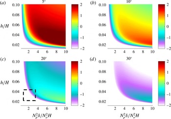
Ratio of steady-state bound harmonic kinetic energy to that of the primary (forcing) internal tide for four latitudes, shown on a logarithmic (base 10) colour scale. Red regions exhibit a significant nonlinear response. The primary internal tide is mode 1, with energy
 $10^{-4}~\text{m}^{2}~\text{s}^{-2}$
. The pycnocline thickness is
 $\unicode[STIX]{x1D6FF}=0.01H$
. The black box in (c) indicates the estimated parameter values corresponding to the South China Sea observations of Xie et al. (Reference Xie, Shang, van Haren and Chen2013).

4 Results
Characteristics of the analytic solution given above are presented here in the context of ocean internal tides, since that is an important application of single-mode internal waves in a bounded domain. The stratification profiles used here have pycnocline depths and thicknesses which are small compared to the water column depth (
 $\unicode[STIX]{x1D6FF}<h\ll H$
), as is typical for ocean conditions. The normalized density change across the pycnocline (
 $g\unicode[STIX]{x0394}\unicode[STIX]{x1D70C}/\unicode[STIX]{x1D70C}N_{o}^{2}H=N_{p}^{2}\unicode[STIX]{x1D6FF}/N_{o}^{2}H$
) is in the range 0.1–10. These parameter values are comparable to realistic ocean stratifications. For computations of time-dependent behaviour, 80 modes are used in (2.10), and an initial condition of
 $\unicode[STIX]{x1D6FF}\unicode[STIX]{x1D713}=0$
is used.
4.1 Steady state
Figure 1 presents the kinetic energy of the steady-state bound harmonic solution as a function of the stratification profile (defined by the pycnocline buoyancy frequency
 $N_{p}$
, depth
 $h$
and thickness
 $\unicode[STIX]{x1D6FF}$
) for
 $4$
latitudes. The primary-mode frequency is fixed at
 $\unicode[STIX]{x1D714}_{o}/N_{o}=0.04$
, corresponding to a semi-diurnal
 $M_{2}$
internal tide (
 $\unicode[STIX]{x1D714}_{o}\simeq 1.4\times 10^{-4}~\text{s}^{-1}$
) in
 $N_{o}=2$
c.p.h. (cycles per hour) stratification (
 $3.5\times 10^{-3}~\text{s}^{-1}$
). The forcing-mode amplitude is set to match the approximate
 $M_{2}$
global mean kinetic energy of
 $\simeq 10^{-4}~\text{m}^{2}~\text{s}^{-2}$
measured by Zhao et al. (Reference Zhao, Alford, Girton, Rainville and Simmons2016), corresponding to horizontal currents of the order of
 $1~\text{cm}~\text{s}^{-1}$
. (Note that
 $M_{2}$
currents an order of magnitude larger are observed in some environments, such as the South China Sea measurements of Xie et al. (Reference Xie, Shang, van Haren and Chen2013).) Rotation frequencies
 $f$
are given in terms of the approximate semi-diurnal frequency
 $\unicode[STIX]{x1D714}_{o}$
and the latitude
 $\unicode[STIX]{x1D703}_{lat}$
by
 $f\simeq \unicode[STIX]{x1D714}_{o}\sin \unicode[STIX]{x1D703}_{lat}$
. The colour scale is logarithmic (base 10). Red indicates regions where the harmonic mode is near resonance, resulting in a significant harmonic response. Since it was assumed here that the primary mode is forced so as to maintain its energy, the solution allows the steady-state bound harmonic-mode energy to exceed that of the primary mode. Of course, this would violate the weakly nonlinear assumption that the harmonic perturbation is small compared to the primary mode, and additional nonlinear effects would become important. If instead the primary mode was not forced, the near-resonance (red) cases would drain significant energy from the primary mode prior to reaching steady state, as in the simulations of Sutherland (Reference Sutherland2016). This scenario is relevant to oceanic internal tides. In either case, the red zones should be interpreted as cases in which the weakly nonlinear approximation would ultimately fail, and a significant harmonic response should be expected. On the other hand, purple and white indicate regions where the harmonic perturbation is expected to remain small, and the weakly nonlinear solution may be approximately valid even for long times.
In figure 1, in any part of parameter space indicating a steady-state bound harmonic energy which is a significant fraction of the primary-mode energy (light blue to red), nonlinear self-interaction could lead to a substantial reduction in the energy of the primary
 $M_{2}$
internal tide. This is most likely when rotation is zero or small and does not occur at latitudes exceeding
 $30^{\circ }$
(not shown). Purple and white areas in figure 1 indicate that the bound harmonic will have at most a few per cent of the energy of the primary mode. Near the Equator (where rotation is weak), these occur only when the pycnocline is either very shallow (
 $h/H<0.02$
) or weak (
 $N_{p}^{2}\unicode[STIX]{x1D6FF}<2N_{o}^{2}H$
). In the latter case, the gradients in
 $N^{2}$
are too small for nonlinear self-interaction to be significant. Elsewhere in the
 $N_{p}-h$
parameter space, a significant harmonic response is possible in equatorial waters. At any given latitude and pycnocline depth
 $h/H$
, the harmonic response generally increases with
 $N_{p}^{2}\unicode[STIX]{x1D6FF}$
. For a fixed value of
 $N_{p}^{2}\unicode[STIX]{x1D6FF}$
, there is a specific pycnocline depth
 $h/H$
where the bound harmonic energy is largest. Away from the Equator, the harmonic mode is farther from resonance, but can still approach the primary-mode energy at
 $30^{\circ }$
latitude for an especially strong, shallow pycnocline.
The small black box in the
 $20^{\circ }$
latitude panel of figure 1 corresponds to the South China Sea observations of Xie et al. (Reference Xie, Shang, van Haren and Chen2013), based on the historical stratification profiles analysed by Wunsch (Reference Wunsch2015). Within this part of parameter space, a harmonic response with 10–20 % of the primary-mode energy could plausibly occur, but the absence of a harmonic is also likely. This is consistent with the intermittent observation of a harmonic mode by Xie et al. (Reference Xie, Shang, van Haren and Chen2013).
For mode 1, significant harmonic responses are found predominantly at latitudes less than
 $10^{\circ }$
. For the example presented in figure 1, the steady-state bound harmonic energy is always less than one per cent of the primary mode at latitudes exceeding
 $45^{\circ }$
(not shown). To see why rotation tends to reduce the harmonic amplitude for mode 1, consider the frequency spectrum
 $\unicode[STIX]{x1D714}(k)$
for a uniform stratification
 $N_{o}$
(i.e. solutions to (3.3) for
 $h=\unicode[STIX]{x1D6FF}=\unicode[STIX]{x1D712}=0$
, which requires
 $qH=\unicode[STIX]{x03C0}$
in (3.7)). The harmonic frequency
 $\unicode[STIX]{x1D714}(2k)$
for mode 1, compared to the primary frequency
 $\unicode[STIX]{x1D714}(k)$
is
 $$\begin{eqnarray}\left(\frac{\unicode[STIX]{x1D714}(2k)}{2\unicode[STIX]{x1D714}(k)}\right)^{2}\simeq \frac{1+\left({\displaystyle \frac{f\unicode[STIX]{x03C0}}{2N_{o}kH}}\right)^{2}}{1+\left({\displaystyle \frac{f\unicode[STIX]{x03C0}}{N_{o}kH}}\right)^{2}}.\end{eqnarray}$$
This reduces to 1, indicating perfect resonance (
 $\unicode[STIX]{x1D714}(2k)=2\unicode[STIX]{x1D714}(k)$
), for
 $f=0$
, but moves away from resonance with rotation (
 $f\neq 0$
). Hence rotation tends to break the near-resonance condition for a mode 1 internal tide forcing. In (3.14), large harmonic amplitudes occur for small
 $D_{o}$
(the denominator of the amplitude coefficients), which occurs for
 $\unicode[STIX]{x1D714}(2k)\simeq 2\unicode[STIX]{x1D714}(k)$
. As
 $f$
increases,
 $D_{o}$
increases as the difference between the harmonic frequency and twice the primary frequency increases. The numerators in (3.14) change with
 $f$
much more slowly, so the increase in the denominator
 $D_{o}$
is primarily responsible for the reduction in steady-state harmonic amplitude as latitude increases.
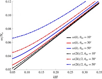
Of course, there is no self-interaction in uniform stratification, and the actual frequency spectrum differs slightly for the non-uniform stratification profiles used here, but the change is not enough to alter the general trend with rotation. This is illustrated in figure 2 for the stratification of (3.1) with
 $h/H=0.04$
,
 $\unicode[STIX]{x1D6FF}/H=0.01$
, and
 $N_{p}^{2}\unicode[STIX]{x1D6FF}/N_{o}^{2}H=2$
. The dispersion relations for three latitudes (assuming
 $N_{o}=2$
cph, as is used throughout) are indicated with solid lines. The corresponding harmonic dispersion relations as a function of
 $2k$
are indicated with dot-dash lines of the same colour. The proximity of these lines indicates the degree of resonance. For small
 $f/N_{o}$
(low latitudes), the harmonic is nearly (but never perfectly) resonant, as indicated by the black lines. Increasing
 $f$
causes the harmonic curve to separate from the forcing mode, as indicated by the red and blue lines, which increases
 $D_{o}$
in (3.14) and reduces the bound harmonic amplitude. This illustrates why significant harmonic generation due to nonlinear self-interaction only occurs in near-equatorial latitudes for the stratification profile of (3.1).
Dispersion relations for several latitudes, for
 $h/H=0.04$
,
 $\unicode[STIX]{x1D6FF}/H=0.01$
and
 $N_{p}^{2}\unicode[STIX]{x1D6FF}/N_{o}^{2}H=2$
. The primary mode
 $\unicode[STIX]{x1D714}(k)$
is shown by solid lines, and the harmonic mode (
 $2k$
) by dot-dashed lines. The proximity of the primary and harmonic dispersion relations indicates the degree of resonance.

In the ocean, most of the energy in the
 $M_{2}$
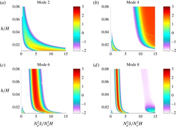
internal tides is contained in mode 1. While mode 1 (figure 1) has a single broad near-resonance band, higher modes exhibit more complicated behaviour, as shown in figure 3. This shows the steady-state bound harmonic energy due to four different primary (forcing) modes, all for a latitude of
 $5^{\circ }$
. The forcing kinetic energy is
 $10^{-6}~\text{m}^{2}~\text{s}^{-2}$
, two orders of magnitude smaller than in figure 1, since in the ocean higher modes are typically much weaker than mode 1. Each forcing mode has a unique wavenumber
 $k$
, and hence a different spectrum of natural frequencies. The alignment of this spectrum with the forcing frequency determines the nonlinear response. Like mode 1, mode 2 has a single band with a large-amplitude bound harmonic. Mode 4 has two such bands within the parameter space shown: a narrow band for small
 $N_{p}^{2}\unicode[STIX]{x1D6FF}$
and a wider band at larger
 $N_{p}^{2}\unicode[STIX]{x1D6FF}$
. In mode 6, these bands shift toward smaller
 $N_{p}^{2}\unicode[STIX]{x1D6FF}$
. Mode 8 has three distinct bands: one at very small
 $N_{p}^{2}\unicode[STIX]{x1D6FF}$
, a stronger response at
 $N_{p}^{2}\unicode[STIX]{x1D6FF}/N_{o}^{2}H\simeq 4$
and a weak band (light blue and purple) at large
 $N_{p}^{2}\unicode[STIX]{x1D6FF}$
. These results illustrate the potentially complicated self-interaction harmonic structure of internal tides in variable stratification. One key observation is that increasing stratification gradients (
 $N_{p}^{2}$
) do not necessarily lead to a more significant harmonic response (despite the larger gradients of
 $N^{2}$
); proximity to natural modes is often more important.
Ratio of steady-state bound harmonic kinetic energy to that of the primary (forcing) internal tide for four different forcing modes, shown on a logarithmic (base 10) colour scale. The primary internal tides have energy
 $10^{-6}~\text{m}^{2}~\text{s}^{-2}$
(smaller than for mode 1 in figure 1). The pycnocline thickness is
 $\unicode[STIX]{x1D6FF}=0.01H$
and the latitude is
 $5^{\circ }$
(
 $f=0.0036N_{o}$
).

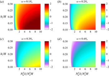
The dependence of the steady-state kinetic energy on the frequency
 $\unicode[STIX]{x1D714}_{o}/N_{o}$
without rotation (
 $f=0$
) is explored in figure 4. Here, parameter values are representative of a typical laboratory facility. The pycnocline is thicker (
 $\unicode[STIX]{x1D6FF}=0.05H$
) and deeper than in the ocean. The results show that increasing the forcing frequency for mode 1 moves the system away from resonance. In a laboratory setting, harmonic generation is best achieved with a low-frequency forcing (
 $\unicode[STIX]{x1D714}_{o}\ll N_{o}$
, corresponding to a near-hydrostatic wave) and a strong, shallow pycnocline.
The steady-state bound harmonic kinetic energy ratio as a function of forcing frequency for conditions typical of a laboratory experiment, with a primary-mode mean kinetic energy of
 $10^{-4}~\text{m}^{2}~\text{s}^{-2}$
,
 $f=0$
and
 $\unicode[STIX]{x1D6FF}/H=0.05$
.

4.2 Early time development
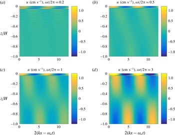
While the previous subsection illustrated the bound harmonic amplitudes that can be generated by nonlinear self-interaction, for ocean applications it is critical to consider how rapidly the harmonic response grows. Figure 5 presents an example of the temporal development of the perturbation to a mode-1 internal tide with the frequency and amplitude of figure 1. The dimensionless pycnocline depth is
 $h/H=0.04$
, its normalized density change is
 $N_{p}^{2}\unicode[STIX]{x1D6FF}/N_{o}^{2}H=2$
and its thickness is
 $\unicode[STIX]{x1D6FF}/H=0.02$
. The initial condition is
 $\unicode[STIX]{x1D6FF}\unicode[STIX]{x1D713}=0$
, and the solution is represented using 80 modes in (2.10). The example shows the wavenumber
 $2k$
perturbation initially emerging near the pycnocline (figure 5
a) as expected since this is where the gradients in
 $N(z)$
are found. By the end of the first forcing period (
 $\unicode[STIX]{x1D714}_{o}t=2\unicode[STIX]{x03C0}$
), the perturbation has grown in vertical extent to cover the full depth of the water column (c). After three forcing periods (d), the perturbation is comparable to the forcing currents (
 ${\sim}2~\text{cm}~\text{s}^{-1}$
) and resembles the spatial structure of the bound harmonic solution (not shown). The harmonic emerges relatively quickly because of the incommensurate frequencies of the natural modes, causing their sum to be relatively incoherent compared to the steady-state bound harmonic.
Growth of the
 $2k$
harmonic-mode horizontal current
 $u=\unicode[STIX]{x2202}_{z}\unicode[STIX]{x1D6FF}\unicode[STIX]{x1D713}$
after 3 periods of the primary mode. Colour bar is in
 $\text{cm s}^{-1}$
.

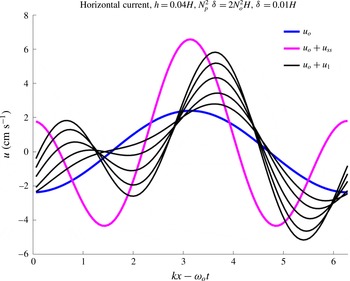
Figure 6 illustrates how the perturbation steepens the internal tide for the same parameters as figure 5. Like the Stokes harmonic of a surface wave, the steady-state solution is a bound harmonic of the forcing mode, moving at the same phase speed and steepening it. The solid blue line in figure 6 shows the forcing-mode horizontal current
 $u_{o}=\unicode[STIX]{x2202}_{z}\unicode[STIX]{x1D713}_{o}$
at the base of the pycnocline (
 $z=-h$
) as a function of horizontal position. The magenta curve shows the steady-state solution
 $u_{o}+u_{s}$
, with a maximum current which is double the unperturbed forcing mode
 $u_{o}$
in this example. The black curves illustrate the time development starting from zero perturbation; the curves are spaced in time by 2 forcing periods. The perturbation grows, approaching the steady-state amplitude after
 $\simeq 10$
periods (highest curve). Subsequently, the solution slightly overshoots the steady state (not shown) and oscillates around it. If viscosity had been included, the solution would have gradually settled to the steady state as the unforced modes damped out.
Horizontal currents at the base of the pycnocline, illustrating the growth of the harmonic mode and steepening of the wave. Each black line is separated by 2 periods. The magenta curve shows the steady-state solution.

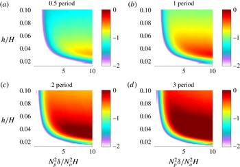
Ratio of harmonic perturbation kinetic energy to that of the primary (forcing) mode 1 internal tide for a latitude of
 $10^{\circ }$
, shown on a logarithmic (base 10) colour scale, for the first 3 periods. The harmonic mode is initially zero. Red indicates a significant energy transfer from the primary mode. The primary-mode internal tide kinetic energy is
 $10^{-4}~\text{m}^{2}~\text{s}^{-2}$
. The pycnocline thickness is
 $\unicode[STIX]{x1D6FF}=0.01H$
.

Of greater interest for ocean applications is the time required for nonlinear self-interaction to remove significant energy from the primary mode. This can be estimated using the present analysis by calculating the kinetic energy in the perturbation as a function of time, using the modal decomposition of (2.10). The initial condition used here,
 $\unicode[STIX]{x1D6FF}\unicode[STIX]{x1D713}=0$
, likely does not apply to the real ocean. This assumption is made to study nonlinear self-interaction in the absence of other effects which may result in a non-zero initial condition for
 $\unicode[STIX]{x1D6FF}\unicode[STIX]{x1D713}$
. Real ocean internal tides propagate across latitudes and changing environments, which have different primary-mode and steady-state bound harmonic solutions
 $\unicode[STIX]{x1D6FF}\unicode[STIX]{x1D713}_{s}$
. The assumed initial condition may be approximately applicable when an internal tide enters an environment in which the steady-state harmonic is much larger in amplitude than the existing perturbation (
 $|\unicode[STIX]{x1D6FF}\unicode[STIX]{x1D713}(t=0)|\ll |\unicode[STIX]{x1D6FF}\unicode[STIX]{x1D713}_{s}|$
). When an internal tide enters an environment in which the steady-state harmonic energy is large, rapid energy transfer to the harmonic mode may occur. Although the removal of energy from the primary mode (the next higher-order term in the weakly nonlinear expansion) is not explicitly modelled, it is clear that the energy is transferred from the primary mode. Once the perturbation energy reaches a significant fraction of the primary-mode energy, additional nonlinear effects become important and self-interaction will begin to dissipate the primary mode.
Figure 7 presents the growth of kinetic energy for a mode 1 internal tide in conditions which are representative of the ocean
 $M_{2}$
internal tide, as in figure 1. The primary-mode energy is
 $10^{-4}~\text{m}^{2}~\text{s}^{-2}$
, the latitude is 10 degrees and the pycnocline thickness is
 $\unicode[STIX]{x1D6FF}=0.01H$
. The results show that the perturbation energy can approach the primary-mode energy after only a single period of the
 $M_{2}$
tide (half a day) in some conditions, and by 3 periods (1.5 days) significant energy extraction is expected over a wide range of parameter space at this latitude. The dependence on rotation is similar to that shown for the steady state; significant energy extraction over a few periods is expected only near the Equator. These results suggest that nonlinear self-interaction may play an important role in the dissipation of
 $M_{2}$
internal tides propagating toward equatorial waters.
5 Discussion
These results illustrate the dynamics of nonlinear self-interaction for the generation of harmonic perturbations to internal tides. A double-wavenumber harmonic is formed, consisting of a superposition of a double-frequency bound harmonic mode and freely propagating modes with other frequencies. Analogous to a forced harmonic oscillator, resonance between the forcing frequency and the freely propagating modes of the system is critical to the dynamics. Near-resonant systems exhibit a significant harmonic response, even for weak forcing. This can alter the dynamics of internal tides which are nearly linear, possibly leading to their dissipation and conversion of energy to smaller scales. The full dynamics near resonance is beyond the scope of the present approach, but non-resonant systems with a weak response can be represented by the weakly nonlinear theory developed here.
Compared to real ocean internal tides, several important simplifications were made. An idealized ocean stratification profile was used. The flow was assumed to be quasi-two dimensional. Only self-interaction was explored; wave–wave interactions with internal tides having other frequencies, modes or directions of propagation were not considered. Effects of topography were not considered.
With these simplifications, weakly nonlinear theory has been used to estimate the possible importance of nonlinear self-interaction to the dissipation of oceanic internal tides. Perfect resonance does not occur, but near-resonant conditions are possible at low latitudes. The results show that, in near-resonant conditions, significant energy transfer may occur in only a few wave periods, but that in non-resonant conditions the effect is likely not important. Geographic and seasonal variations in dissipation would therefore be expected. Changing conditions could cause harmonics to grow and decay, as in the observations of Xie et al. (Reference Xie, Shang, van Haren and Chen2013). Harmonics with significant amplitude appear most probable in equatorial oceans, as rotation tends to weaken the effect.
Real oceanic internal tides propagate across latitudes, and the present results indicate that propagation toward the Equator could bring a mode with an initially weak harmonic perturbation closer to resonance conditions, resulting in increased energy transfer to the harmonic mode. Significant energy transfer could plausibly occur in less than one day, possibly resulting in the dissipation of the primary mode. This may explain the energy loss in mode 1
 $M_{2}$
tides in Pacific equatorial waters observed by Zhao et al. (Reference Zhao, Alford, Girton, Rainville and Simmons2016). Future work will explore this dynamics using fully nonlinear simulations and more realistic stratification profiles.
It should be straightforward to extend this approach to arbitrary stratification profiles by computing eigenmodes numerically. This would permit calculation of the expected harmonic response due to nonlinear self-interaction for real ocean stratification profiles. Such results could guide future observations as well as laboratory and numerical experiments.
The sensitivity of nonlinear self-interaction to stratification profiles suggests the possibility that, as climate changes, varying stratification profiles might alter the locations and/or seasons at which near resonance is likely. For instance, increased heating of the upper ocean may result in stronger pycnoclines and larger gradients in buoyancy frequency. This could change the mixing and energy transfer from low-mode internal tides due to nonlinear self-interaction.
Acknowledgement
The author gratefully acknowledges helpful discussions and suggestions from Professor P. Diamessis.