1 Introduction
Animal flight is the result of intertwined complex mechanisms, including sensory feedback and neural control, muscular morphology and actuation, and wing kinematics and aerodynamics, all combined to produce remarkable flight agility and robustness. Developing an understanding of flapping flight at each of these layers presents its unique challenges. At the flight mechanics level, the unsteady flow generated by flapping wings is responsible for the lift and thrust forces that allow insects and birds to fly forwards or hover in place. The production of these lift and thrust forces by leading edge and wake vorticity has been addressed in numerous experimental and numerical studies; see, for example, Ellington et al. (Reference Ellington, van den Berg, Willmott and Thomas1996), Dickinson, Lehmann & Sane (Reference Dickinson, Lehmann and Sane1999), Minotti (Reference Minotti2002), Ramamurti & Sandberg (Reference Ramamurti and Sandberg2002), Birch & Dickinson (Reference Birch and Dickinson2003), Sane (Reference Sane2003), Spedding, Rosén & Hedenström (Reference Spedding, Rosén and Hedenström2003), Sun & Lan (Reference Sun and Lan2004), Thomas et al. (Reference Thomas, Taylor, Srygley, Nudds and Bomphrey2004), Wang (Reference Wang2005).
Passively flying bodies, that is to say, bodies moving solely under the influence of gravitational and aerodynamic forces with no internal actuation, have been proposed as surrogates to the flapping flight problem; see, for example, Jones (Reference Jones2003), Andersen, Pesavento & Wang (Reference Andersen, Pesavento and Wang2005a ,Reference Andersen, Pesavento and Wang b ), Jones & Shelley (Reference Jones and Shelley2005), Alben (Reference Alben2010). The substitution of the active flight problem by a passive analogue can be particularly attractive because it simplifies the study of fluid–structure interactions. However, such substitution is only beneficial when the vortical structures in the passive problem are similar to those shed in the active flapping problem. To this end, an ingenious model system of an inanimate flyer consisting of an upward-pointing pyramid-shaped object in a vertically oscillating airflow was recently proposed in Childress, Vandenberghe & Zhang (Reference Childress, Vandenberghe and Zhang2006), Weathers et al. (Reference Weathers, Folie, Liu, Childress and Zhang2010). The inanimate pyramid generates aerodynamic forces and moments that keep it aloft and passively balanced during free flight (Liu et al. Reference Liu, Ristroph, Weathers, Childress and Zhang2012). A quasisteady theory based upon shape-related drag in steady flows is employed in Weathers et al. (Reference Weathers, Folie, Liu, Childress and Zhang2010) to estimate the dependence of the lift force on the pyramid’s geometric properties. While capable of qualitatively capturing the effect of geometric asymmetry, the quasisteady theory significantly underestimates the lift provided by the oscillating airflow. Note that without shed vorticity no lift is possible (Weathers et al. Reference Weathers, Folie, Liu, Childress and Zhang2010). Thus, to properly account for the lift forces, it is necessary to compute the evolution of the shed vorticity and its contribution to the aerodynamic forces acting on the flyer.
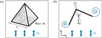
Inspired by the experimental study of Weathers et al. (Reference Weathers, Folie, Liu, Childress and Zhang2010), we consider here a two-dimensional, up-down asymmetric flyer hovering in an oscillating uniform flow; see figure 1. The flyer consists of two flat ‘wings’ connected rigidly at their apex to form a
 $\unicode[STIX]{x039B}$
-flyer. We account for the aerodynamic effects using a vortex sheet model in the inviscid fluid context; see, for example, Krasny (Reference Krasny1986), Nitsche & Krasny (Reference Nitsche and Krasny1994), Jones (Reference Jones2003), Jones & Shelley (Reference Jones and Shelley2005), Shukla & Eldredge (Reference Shukla and Eldredge2007). We use this modelling framework to compute the two-way coupling between the flyer and the shed vorticity, and thus examine the unsteady flow–structure interactions as opposed to the quasistatic analysis in Weathers et al. (Reference Weathers, Folie, Liu, Childress and Zhang2010). In particular, we present a detailed study of the inter-dependence between the flyer’s inertia and geometric characteristics and the requirements on the oscillatory flow to ensure hovering.
Sketch of (a) pyramid hovering in vertically oscillatory flows with zero mean as in Weathers et al. (Reference Weathers, Folie, Liu, Childress and Zhang2010); and (b) model system of a
 $\unicode[STIX]{x039B}$
-shaped flyer subject to gravity in oscillating flow.

The paper is organized as follows. Section 2 presents the mathematical formulation simulating a flyer moving freely in oscillatory flows. The flyer’s motion is based on the balance of linear and angular momenta, while the fluid–structure interactions are based on a vortex sheet model. The resulting scheme is validated against two studies of flat plates in still and oscillating flows (Jones Reference Jones2003; Jones & Shelley Reference Jones and Shelley2005). In § 3, the response of the
 $\unicode[STIX]{x039B}$
-flyer in oscillatory flows is investigated numerically, and the numerical results are compared to the experimental results of Weathers et al. (Reference Weathers, Folie, Liu, Childress and Zhang2010). We find that, under certain conditions on flow frequencies or speeds, the flow acceleration, which one could interpret as a measure of the aerodynamic effort required to hover as done in Huang, Nitsche & Kanso (Reference Huang, Nitsche and Kanso2015), is an intrinsic property of the flyer itself. More specifically, for these conditions, a given flyer of fixed mass and shape requires a constant amount of effort to hover, irrespective of the amplitude and frequency of oscillation of the background flow. The implications of our results on passive and active flight are discussed in § 4.
2 Model
2.1 The
 $\unicode[STIX]{x039B}$
-flyer

Consider a two-dimensional
 $\unicode[STIX]{x039B}$
-flyer of total mass
 $M$
consisting of two flat plates, each of length
 $l$
, joined at the apex with an opening angle
 $2\unicode[STIX]{x1D6FC}$
, as shown in figure 1(b). The plates are homogeneous so that the centre of mass
 $C$
is located on the flyer’s axis of symmetry. The gravitational force acts vertically on the plate with magnitude
 $Mg$
, where
 $g$
is the gravitational constant. The background fluid has density
 $\unicode[STIX]{x1D70C}_{f}$
and oscillates vertically with velocity
 $U(t)=A(\unicode[STIX]{x03C0}f)\text{sin}(2\unicode[STIX]{x03C0}f\,t)$
, where
 $f$
is the oscillation frequency,
 $A$
is the peak-to-peak oscillation amplitude, and
 $t$
is time.
The problem is described in the complex
 $z$
-plane. Let
 $z_{c}=x_{c}+\text{i}y_{c}$
denote the position of the centre of mass
 $C$
of the
 $\unicode[STIX]{x039B}$
-flyer and
 $\unicode[STIX]{x1D703}$
denote its orientation from the upward vertical, being positive in the counterclockwise direction. The equations governing the evolution of
 $z_{c}$
and
 $\unicode[STIX]{x1D703}$
, and thereby the flyer’s motion under gravitational and aerodynamic effects, are given by the balance of linear and angular momenta on the flyer, namely,
 $$\begin{eqnarray}M\ddot{z}_{c}=F_{x}+\text{i}(F_{y}-Mg),\quad I\ddot{\unicode[STIX]{x1D703}}=\unicode[STIX]{x1D70F}_{c}.\end{eqnarray}$$
Here,
 $I=Ml^{2}(1-(3/4)\cos ^{2}(\unicode[STIX]{x1D6FC}))/3$
is the flyer’s moment of inertia with respect to the centre of mass, and
 $F_{x}$
,
 $F_{y}$
and
 $\unicode[STIX]{x1D70F}_{c}$
are the aerodynamic forces and torque exerted by the surrounding fluid on the flyer.
The flow is non-dimensionalized using
 $l$
,
 $T=1/f$
and
 $\unicode[STIX]{x1D70C}_{f}$
as the length, time, and density scales, respectively. Non-dimensional analysis yields four independent, dimensionless parameters: the opening angle
 $\unicode[STIX]{x1D6FC}$
and mass
 $m$
of the flyer, and the amplitude and acceleration
 $\unicode[STIX]{x1D6FD}$
and
 $\unicode[STIX]{x1D705}$
of the background flow (Liu et al.
Reference Liu, Ristroph, Weathers, Childress and Zhang2012),
 $$\begin{eqnarray}\unicode[STIX]{x1D6FC},\quad m=M/\unicode[STIX]{x1D70C}_{f}l^{2},\quad \unicode[STIX]{x1D6FD}=A/l,\quad \unicode[STIX]{x1D705}=Af^{2}/g.\end{eqnarray}$$
All remaining parameters and variables are also non-dimensionalized in terms of
 $l,f,\unicode[STIX]{x1D70C}_{f}$
such that
 $\tilde{z}=z/l$
,
 $\tilde{t}=ft$
,
 $\tilde{I} =I/(\unicode[STIX]{x1D70C}_{f}l^{4})=m(1-(3/4)\cos ^{2}(\unicode[STIX]{x1D6FC}))/3$
,
 $\tilde{F}_{x}=F_{x}/(\unicode[STIX]{x1D70C}_{f}l^{3}f^{2})$
, etc. Hereafter, we drop the tilde notation with the understanding that all variables are non-dimensional. The resulting non-dimensionalized equations of motion are
 $$\begin{eqnarray}m\ddot{z}_{c}=F_{x}+\text{i}\left(F_{y}-\frac{m\unicode[STIX]{x1D6FD}}{\unicode[STIX]{x1D705}}\right),\quad I\ddot{\unicode[STIX]{x1D703}}=\unicode[STIX]{x1D70F}_{c},\end{eqnarray}$$
with non-dimensional oscillatory background flow velocity
 $$\begin{eqnarray}U(t)=\unicode[STIX]{x03C0}\unicode[STIX]{x1D6FD}\sin (2\unicode[STIX]{x03C0}t).\end{eqnarray}$$
2.2 The vortex sheet model
The coupled fluid–structure interaction between the plate and the surrounding fluid is simulated using an inviscid vortex sheet model. The resulting fluid motion yields the aerodynamic forces and moment
 $F_{x}$
,
 $F_{y}$
and
 $\unicode[STIX]{x1D70F}_{c}$
that determine the motion of the flyer.
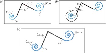
Vortex sheet model for the
 $\unicode[STIX]{x039B}$
-shaped flyer. (a) Sketch showing bound vortex sheet
 $l_{b}$
and free sheets
 $l_{l,r}$
, parametrized by
 $z_{b}(s,t)$
and
 $z_{l,r}(\unicode[STIX]{x1D6E4},t)$
respectively. (b) Sketch showing contour
 $C_{n}$
, shed circulations
 $\unicode[STIX]{x1D6E4}_{l,r}$
, and the tangential velocity components and pressure above and below the bound sheet. (c) Discretization of bound and free vortex sheets by
 $2n+1$
point vortices (bound sheet) and
 $n^{l,r}$
regularized vortices (left and right free sheets).

A sketch of the vortex sheet model is shown in figure 2. The flyer is approximated by a bound vortex sheet, denoted by
 $l_{b}$
, whose strength ensures that no fluid flows through the rigid walls, see figure 2(a). In viscous flow, the surrounding fluid velocity induces the formation of boundary layer vorticity along the sides of the flyer, that is swept away from the flyer at the two sharp ends and forms a shear layer that rolls up into vortices. In the model, the separated shear layers are approximated by free regularized vortex sheets
 $l_{l}$
and
 $l_{r}$
attached to the left and right ends, respectively. The total shed circulation
 $\unicode[STIX]{x1D6E4}_{l}$
and
 $\unicode[STIX]{x1D6E4}_{r}$
in each of the two sheets is determined so as to satisfy the Kutta condition at the edges, which is given in terms of the tangential velocity components above and below the bound sheet and ensures that the pressure jump across the sheet vanishes at the edges, see figure 2(b). Such a regularized vortex sheet method has been applied to study a number of problems in fluid–structure interactions, including vortex ring formation at the edge of a circular tube (Nitsche & Krasny Reference Nitsche and Krasny1994), vortex shedding around an oscillating flat plate (Jones Reference Jones2003), and the motion of falling cards (Jones & Shelley Reference Jones and Shelley2005) and flapping flexible flags (Alben & Shelley Reference Alben and Shelley2008; Alben Reference Alben2009). All essential components for the present model are summarized herein.
The bound vortex sheet
 $l_{b}$
is described by its position, parametrized as
 $z_{b}(s,t),s\in [-l,l]$
, and its sheet strength
 $\unicode[STIX]{x1D6FE}(s,t)$
, where
 $s$
denotes the arclength along the sheet
 $l_{b}$
. The two separated sheets
 $l_{l}$
and
 $l_{r}$
are described by their position, parametrized as
 $z_{l}(\unicode[STIX]{x1D6E4},t)$
,
 $\unicode[STIX]{x1D6E4}\in [0,\unicode[STIX]{x1D6E4}_{l}]$
and
 $z_{r}(\unicode[STIX]{x1D6E4},t)$
,
 $\unicode[STIX]{x1D6E4}\in [0,\unicode[STIX]{x1D6E4}_{r}]$
, where
 $\unicode[STIX]{x1D6E4}$
is the Lagrangian circulation around the portion of the separated sheet between its free end in the spiral centre and the point
 $z(\unicode[STIX]{x1D6E4},t)$
. The parameter
 $\unicode[STIX]{x1D6E4}$
defines the vortex sheet strength
 $\unicode[STIX]{x1D6FE}=\text{d}\unicode[STIX]{x1D6E4}/\text{d}s$
.
By linearity of the problem, the complex velocity
 $w(z,t)=u(z,t)-\text{i}v(z,t)$
is a superposition of the contributions due to the three vortex sheets as well as the external background flow
 $$\begin{eqnarray}w(z,t)=w_{f}(z,t)+w_{b}(z,t)+w_{ext}(z,t).\end{eqnarray}$$
Here,
 $w_{f}(z,t)$
and
 $w_{b}(z,t)$
are the velocity components induced by the free and bound vortex sheets respectively, and
 $w_{ext}(t)$
is the background velocity. In practice, the free sheet is regularized using the vortex blob method to prevent the growth of the Kelvin–Helmholtz instability. The bound sheet is not regularized in order to preserve the invertibility of the map between the sheet strength and the normal velocity along the sheet. The resulting velocity components are given by
 $$\begin{eqnarray}\left.\begin{array}{@{}c@{}}\displaystyle w_{b}(z,t)=\int _{-l}^{l}K_{0}(z-z_{b}(s,t))\unicode[STIX]{x1D6FE}(s,t)\,\text{d}s,\\ \displaystyle w_{f}(z,t)=\int _{0}^{\unicode[STIX]{x1D6E4}_{l}}K_{\unicode[STIX]{x1D6FF}}(z-z_{l}(\unicode[STIX]{x1D6E4},t))\,\text{d}\unicode[STIX]{x1D6E4}+\int _{0}^{\unicode[STIX]{x1D6E4}_{r}}K_{\unicode[STIX]{x1D6FF}}(z-z_{r}(\unicode[STIX]{x1D6E4},t))\,\text{d}\unicode[STIX]{x1D6E4},\\ \displaystyle w_{ext}(z,t)=-\text{i}U(t),\end{array}\right\}\end{eqnarray}$$
where
 $$\begin{eqnarray}K_{\unicode[STIX]{x1D6FF}}(z)=\frac{1}{2\unicode[STIX]{x03C0}\text{i}}\frac{\overline{z}}{|z|^{2}+\unicode[STIX]{x1D6FF}^{2}}\end{eqnarray}$$
is the vortex blob kernel. If
 $z$
is a point on the bound sheet,
 $w_{b}$
is to be computed in the principal value sense.
The position of the bound vortex sheet
 $z_{b}$
representing the flyer is given by its centre of mass
 $z_{c}$
and orientation
 $\unicode[STIX]{x1D703}$
, which is determined by (2.3). The corresponding sheet strength
 $\unicode[STIX]{x1D6FE}(s,t)$
is determined by imposing the no-penetration boundary condition on the flyer, together with conservation of total circulation. If
 $n(s,t)=n_{1}+\text{i}n_{2}$
is the upward complex normal to the flyer, the no-penetration condition is
 $$\begin{eqnarray}\text{Re}\,[wn]=\text{Re}\,[w_{flyer}n],\end{eqnarray}$$
at all points
 $z_{b}(s,t)$
, where
 $$\begin{eqnarray}w_{flyer}(z_{b},t)=\dot{\bar{z}}_{c}(t)+\text{i}\dot{\unicode[STIX]{x1D703}}(\bar{z}_{c}(t)-\bar{z}_{b})\end{eqnarray}$$
is the flyer’s complex velocity. Conservation of the fluid circulation implies that
 $$\begin{eqnarray}\unicode[STIX]{x1D6E4}_{l}(t)+\int _{l_{b}}\unicode[STIX]{x1D6FE}_{b}(s,t)\,\text{d}s+\unicode[STIX]{x1D6E4}_{r}(t)=0.\end{eqnarray}$$
The circulation parameter
 $\unicode[STIX]{x1D6E4}$
along the free vortex sheets
 $z_{l,r}(\unicode[STIX]{x1D6E4},t)$
is determined by the circulation shedding rates
 $\dot{\unicode[STIX]{x1D6E4}}_{l,r}$
. These are given by the Kutta condition, which states that the fluid velocity at the edge be finite and tangent to the flyer. The Kutta condition can be obtained from the Euler equations by enforcing that the difference between the pressure above and below the flyer be zero at the edges, as follows. Integration of the balance of momentum equation for inviscid planar flow, along a closed contour
 $C_{n}$
defined in figure 2(b), yields that
 $$\begin{eqnarray}[p]_{\mp }(s)=p_{-}(s)-p_{+}(s)=-\frac{\text{d}\unicode[STIX]{x1D6E4}(s,t)}{\text{d}t}-\frac{1}{2}(u_{-}^{2}-u_{+}^{2}),\end{eqnarray}$$
where
 $\unicode[STIX]{x1D6E4}(s,t)=\unicode[STIX]{x1D6E4}_{l}+\int _{-l}^{s}\unicode[STIX]{x1D6FE}(s^{\prime },t)\,\text{d}s^{\prime }$
,
 $-l\leqslant s\leqslant l$
, is the circulation within the contour
 $C_{n}$
and
 $p_{\mp }(s,t)$
and
 $u_{\mp }(s,t)$
denote the limiting pressure and tangential slip velocities below and above the flyer, as shown in figure 2(b). Since the pressure difference across the free sheets is zero, it also vanishes at the edges by continuity, which implies that
 $$\begin{eqnarray}\dot{\unicode[STIX]{x1D6E4}}_{l,r}=\mp {\textstyle \frac{1}{2}}(u_{-}^{2}-u_{+}^{2})|_{s=\mp l}.\end{eqnarray}$$
The values of
 $u_{-}$
and
 $u_{+}$
necessary to evaluate (2.12) are obtained from the average tangential velocity component and from the velocity jump at the edges, given by the sheet strength,
 $$\begin{eqnarray}\overline{u}=\frac{u_{+}+u_{-}}{2}=\text{Im}\,[(w-w_{flyer})n],\quad u_{-}-u_{+}=\unicode[STIX]{x1D6FE},\end{eqnarray}$$
evaluated at
 $s=\mp l$
. Once shed, the vorticity in the free sheet moves with the flow. Thus the parameter
 $\unicode[STIX]{x1D6E4}$
assigned to each particle
 $z_{l,r}(\unicode[STIX]{x1D6E4},t)$
is the value of
 $\unicode[STIX]{x1D6E4}_{l,r}$
at the instant it is shed from the edge. The evolution of the free vortex sheets
 $z_{l,r}$
is obtained by advecting it in time with the fluid velocity,
 $$\begin{eqnarray}\dot{\bar{z}}_{l,r}=w_{f}(z_{l,r},t)+w_{b}(z_{l,r},t)+w_{ext}(t).\end{eqnarray}$$
To close the equations of motion of the flyer (2.3), we need to calculate the aerodynamic forces and moment. In inviscid fluid, the aerodynamic forces and moment are determined entirely from the pressure difference in (2.11), with
 $$\begin{eqnarray}\left.\begin{array}{@{}c@{}}\displaystyle F_{x}+\text{i}F_{y}=\int _{l_{b}}n[p]_{\mp }(s)\,\text{d}s,\\ \displaystyle \unicode[STIX]{x1D70F}_{c}=-\text{Re}\,\left[\int _{l_{b}}\text{i}\overline{n}(z_{c}-z_{b}(s))[p]_{\mp }(s)\,\text{d}s\right],\end{array}\right\}\end{eqnarray}$$
where, as before,
 $n=n_{1}+\text{i}n_{2}$
is a complex upward normal to the flyer. The set of equations (2.3)–(2.15) form a closed system of integral–differential equations for solving for the motion of a
 $\unicode[STIX]{x039B}$
-flyer in oscillatory flows.
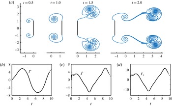
Flat plate oscillating in direction normal to itself with position
 $x_{pl}(t)=-\!\cos (\unicode[STIX]{x03C0}t)$
. (a) Solution at indicated times, computed with
 $\unicode[STIX]{x1D6FF}=0.2$
,
 $n=32$
,
 $\unicode[STIX]{x0394}t=0.004$
. (b–d) Corresponding shed circulation
 $\unicode[STIX]{x1D6E4}(t)$
, circulation shedding rate
 $\dot{\unicode[STIX]{x1D6E4}}(t)$
, and generated force
 $F_{x}$
, where
 $\unicode[STIX]{x1D6E4}=\unicode[STIX]{x1D6E4}_{r}=-\unicode[STIX]{x1D6E4}_{l}$
. The present results are shown in solid lines, the results of Jones (Reference Jones2003) are shown in dashed lines.

2.3 Numerical implementation
The bound vortex sheet is discretized by
 $2n+1$
point vortices at
 $z_{j}^{b}(t)$
with strength
 $\unicode[STIX]{x0394}\unicode[STIX]{x1D6E4}_{j}=\unicode[STIX]{x1D6FE}_{j}\unicode[STIX]{x0394}s_{j}$
, as illustrated in figure 2(c). These vortices are located at Chebyshev points that cluster at the ends and at the apex of the flyer. Their strength is determined by enforcing no penetration at the midpoints between the vortices, together with conservation of circulation. The free sheets are discretized by regularized point vortices at
 $z_{j}^{l,r}(t)$
, that are released from the edge at each time step with circulation given by (2.12). The free point vortices move with the discretized fluid velocity (2.14), while the bound vortices move with the flyer’s velocity, given by (2.3). The discretization of equations (2.3), (2.12), (2.14) yields a coupled system of ordinary differential evolution equations for the flyer’s position, the shed circulations, and the free vorticity, that is integrated in time using the fourth-order Runge–Kutta scheme. The details of the shedding algorithm are given in Nitsche & Krasny (Reference Nitsche and Krasny1994). The numerical values of the time step
 $\unicode[STIX]{x0394}t$
, the number of bound vortices
 $n$
, and the regularization parameter
 $\unicode[STIX]{x1D6FF}$
are chosen so that the solution changes little under further refinement.
Finally, to emulate the effect of viscosity, we allow the shed vortex sheets to decay gradually by dissipating each incremental point vortex after a finite time
 $T_{diss}$
from the time it is shed into the fluid. Larger
 $T_{diss}$
implies that the vortices stay in the fluid for longer times, mimicking the effect of lower fluid viscosity. A closed-form expression that rigorously links
 $T_{diss}$
to the kinematic fluid viscosity is not readily available; however, using approximate arguments based on the Lamb–Oseen solution (Lamb Reference Lamb1932; Jing, Kanso & Newton Reference Jing, Kanso and Newton2010), we choose
 $T_{diss}$
such that
 $\unicode[STIX]{x1D708}T_{diss}$
is small, where
 $\unicode[STIX]{x1D708}$
is the normalized viscosity of air. The effect of
 $T_{diss}$
on the behaviour of the flyer in comparison to the experimental data of Weathers et al. (Reference Weathers, Folie, Liu, Childress and Zhang2010) is reported and discussed in Huang et al. (Reference Huang, Nitsche and Kanso2015).
2.4 Validation of the numerical method
To validate the numerical scheme, we examine two examples of a flat plate (
 $\unicode[STIX]{x1D6FC}=90^{\circ }$
) interacting with background fluid and compare the results with previous work in Jones (Reference Jones2003), Jones & Shelley (Reference Jones and Shelley2005). In the first example, a flat plate of half-length
 $l=1$
oscillates in direction normal to itself with position
 $x_{pl}(t)=-\!\cos (\unicode[STIX]{x03C0}t)$
. We compute the induced flow in a reference frame fixed on the plate by setting
 $U_{ext}=-U(t)$
, using
 $\unicode[STIX]{x1D6FF}=0.2$
,
 $n=32$
,
 $\unicode[STIX]{x0394}t=0.004$
. This problem was simulated in Jones (Reference Jones2003), also using a vortex sheet model. However, the implementation details of the Kutta condition differ significantly from our present approach. At early times, Jones (Reference Jones2003) uses an asymptotic solution to the full system of evolution equations. At later times, the Kutta condition is satisfied by explicitly enforcing that the complex velocity at the tip be finite. Figure 3(a) shows the solution computed with the present method at the indicated times. The results are indistinguishable from those presented in Jones (Reference Jones2003), in figure 6 therein. Figure 3(b–d) shows the shed circulation
 $\unicode[STIX]{x1D6E4}(t)$
, the circulation shedding rate
 $\dot{\unicode[STIX]{x1D6E4}}(t)$
, and the induced aerodynamic force in the horizontal direction
 $F_{x}$
. The results computed with the present method, shown here as a solid line, are basically indistinguishable from those presented in Jones (Reference Jones2003), shown here as a dashed line, illustrating that the two differing implementations of the Kutta condition are equally accurate.
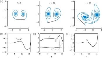
Flat plate with
 $m=2$
and initial orientation
 $\unicode[STIX]{x1D703}=\unicode[STIX]{x03C0}/256$
, freely falling in fluid under gravity and initially at rest. (a) Solution at the indicated times, computed with
 $\unicode[STIX]{x1D6FF}=0.2$
,
 $n=40$
, and
 $\unicode[STIX]{x0394}t=0.004$
. Corresponding (b) total shed circulation
 $\unicode[STIX]{x1D6E4}_{l}+\unicode[STIX]{x1D6E4}_{r}$
, (c) unsteady horizontal and vertical forces
 $F_{x},F_{y}$
and (d) torque
 $\unicode[STIX]{x1D70F}_{c}$
exerted on the plate as function of time. Time scales are normalized by
 $\sqrt{l/g}$
.

Figure 4 shows results for the second example of vortex shedding around a freely falling plate. Following the work of Jones & Shelley (Reference Jones and Shelley2005), the plate has non-dimensional mass
 $m=2$
and initial orientation
 $\unicode[STIX]{x1D703}=\unicode[STIX]{x03C0}/256$
, slightly perturbed from the horizontal. Figure 4(a) shows the solution at the indicated times, normalized by
 $\sqrt{l/g}$
. The initial perturbation causes asymmetric vortex shedding on the left and right sides of the plate. This asymmetry grows in time, as quantified by the total shed circulation
 $\unicode[STIX]{x1D6E4}_{l}+\unicode[STIX]{x1D6E4}_{r}$
, shown in figure 4(b). The resultant unsteady aerodynamic forces and torque also fluctuate with increasing amplitude, see figure 4(c,d). The falling motion is thus unstable due to unsteady vortex shedding, given that added mass effects alone stabilize broadside-on falling motion (Michelin & Smith Reference Michelin and Smith2009). All results are in excellent agreement with the results reported in Jones & Shelley (Reference Jones and Shelley2005).
3 Results
We now examine the dynamics of a
 $\unicode[STIX]{x039B}$
-flyer subject to gravitational and aerodynamic forces in oscillatory background flows. We solve for the flyer’s motion following the steps described in § 2.3 using
 $\unicode[STIX]{x1D6FF}=0.1$
,
 $n=40$
and
 $\unicode[STIX]{x0394}t=0.001$
. The dissipation time parameter is set to
 $T_{diss}=0.7T$
, where the dimensionless oscillation period
 $T$
is equal to one.
Consider a flyer of mass
 $m=8$
and opening angle
 $\unicode[STIX]{x1D6FC}=60^{\circ }$
in an oscillating background flow with
 $\unicode[STIX]{x1D6FD}=1$
and
 $\unicode[STIX]{x1D705}=4$
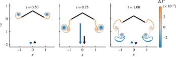
. Figure 5 shows snapshots of the vortex shedding and flyer position for symmetric initial conditions:
 $\unicode[STIX]{x1D703}(0)=\dot{\unicode[STIX]{x1D703}}(0)=0$
and
 $x_{c}(0)=y_{c}(0)=0$
. It is worth noting here that, for this value of
 $\unicode[STIX]{x1D6FC}$
, we do not enforce symmetry in our simulations because the flyer’s motion is stable. However, in later simulations with smaller values of
 $\unicode[STIX]{x1D6FC}$
, we do enforce
 $\unicode[STIX]{x1D703}=0$
for all time. This enforcement of
 $\unicode[STIX]{x1D703}=0$
is analogous to tethering the flyer and restricting it to move along the vertical direction, as done experimentally in Weathers et al. (Reference Weathers, Folie, Liu, Childress and Zhang2010). Counterclockwise vortices are shown in red and clockwise vortices in blue. At the end of one oscillation period, two vortex dipoles form at the two outer edges of the flyers and move downwards. By conservation of linear momentum of the whole fluid–flyer system, the downward momentum of the vortex dipoles is counteracted by a lift force that keeps the flyer aloft, as noted qualitatively in Liu et al. (Reference Liu, Ristroph, Weathers, Childress and Zhang2012). The flyer’s vertical position
 $y_{c}$
, circulation
 $\unicode[STIX]{x1D6E4}_{l,r}$
shed at the left and right corners, and lift force
 $F_{y}$
are quantified in the highlighted plots of figures 6 and 7.
Snapshots of
 $\unicode[STIX]{x039B}$
-flyer and its wake at indicated times. Parameter values are:
 $\unicode[STIX]{x1D6FC}=60^{\circ }$
,
 $m=8$
,
 $\unicode[STIX]{x1D6FD}=1$
,
 $\unicode[STIX]{x1D705}=4$
and
 $T_{diss}=0.7T$
. Initial conditions are:
 $x_{c}(0)=y_{c}(0)=0$
,
 ${\dot{x}}_{c}(0)={\dot{y}}_{c}(0)=0$
and
 $\unicode[STIX]{x1D703}(0)=\dot{\unicode[STIX]{x1D703}}(0)=0$
. Black and blue arrows in the left corner refer to the velocities of the flyer and background flow, respectively.

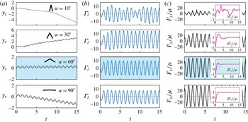
Figure 6 compares the response of several flyers that differ only in shape; namely, the opening angle
 $\unicode[STIX]{x1D6FC}$
varies from
 $10^{\circ }$
to
 $90^{\circ }$
. The flyer’s vertical position
 $y_{c}$
oscillates in time at the same frequency as the background flow oscillations, but may also drift either downwards (descend) or upwards (ascend), or hover in place, depending on the value of
 $\unicode[STIX]{x1D6FC}$
. Note that the dependence on
 $\unicode[STIX]{x1D6FC}$
is nonlinear in the sense that as
 $\unicode[STIX]{x1D6FC}$
increases, the flyer first descends, then ascends, hovers and descends again. To quantify the net drift in the flyer’s vertical position, we consider the
 $T$
-averaged position
 $\langle y_{c}\rangle =(1/T)(\int _{t}^{t+T}y_{c}(t^{\prime })\,\text{d}t^{\prime })$
, depicted in grey in figure 6(a). The numerical results in figure 6(a) show that, after some transience, the net drift is linear, that is,
 $\langle y_{c}\rangle$
depends linearly on time. When comparing the hovering case
 $\unicode[STIX]{x1D6FC}=60^{\circ }$
to the descending case
 $\unicode[STIX]{x1D6FC}=90^{\circ }$
, one sees that the effect of shape on the shed circulation
 $\unicode[STIX]{x1D6E4}_{l,r}$
and vertical aerodynamic force
 $F_{y}$
is subtle. The aerodynamic force
 $F_{y}$
normalized by the flyer’s weight
 $\unicode[STIX]{x1D707}=m\unicode[STIX]{x1D6FD}/\unicode[STIX]{x1D705}$
oscillates such that, after some transient, its
 $T$
-averaged value
 $\langle F_{y}\rangle /\unicode[STIX]{x1D707}$
approaches one in both cases. This is consistent with the observation that the long-term behaviour of
 $\langle y_{c}\rangle$
is linear in time, indicating that
 $m\langle \ddot{y} _{c}\rangle =0=\langle F_{y}\rangle -\unicode[STIX]{x1D707}$
, hence,
 $\langle F_{y}\rangle /\unicode[STIX]{x1D707}=1$
.
 $\unicode[STIX]{x039B}$
-flyer of different opening angle
 $\unicode[STIX]{x1D6FC}$
ranging from
 $10^{\circ }$
to
 $90^{\circ }$
. Parameter values are:
 $m=8$
,
 $\unicode[STIX]{x1D6FD}=1$
,
 $\unicode[STIX]{x1D705}=4$
and
 $T_{diss}=0.7T$
. (a)
 $y_{c}$
(black line) and its
 $T$
-averaged value (grey line) versus time. (b) Circulation
 $\unicode[STIX]{x1D6E4}_{l}$
versus time,
 $\unicode[STIX]{x1D6E4}_{r}=-\unicode[STIX]{x1D6E4}_{l}$
. (c) Vertical aerodynamic force
 $F_{y}$
normalized by the flyer’s weight
 $\unicode[STIX]{x1D707}=m\unicode[STIX]{x1D6FD}/\unicode[STIX]{x1D705}$
versus time.
 $T$
-averaged force
 $\langle F_{y}\rangle /\unicode[STIX]{x1D707}$
approaches 1, shown in the inset. The highlighted case corresponds to the one shown in figure 5.

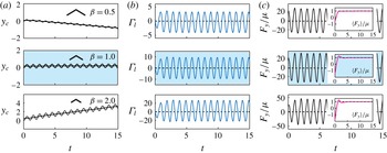
 $\unicode[STIX]{x039B}$
-flyer of
 $\unicode[STIX]{x1D6FD}=A/l=0.5,1,2$
. Parameter values are:
 $m=8$
,
 $\unicode[STIX]{x1D6FC}=60^{\circ }$
,
 $\unicode[STIX]{x1D705}=4$
and
 $T_{diss}=0.7T$
. (a)
 $y_{c}$
(black line) and its
 $T$
-averaged value (grey line) versus time. (b) Circulation
 $\unicode[STIX]{x1D6E4}_{l}$
versus time. (c) Normalized aerodynamic force
 $F_{y}/\unicode[STIX]{x1D707}$
and its
 $T$
-averaged value versus time. The highlighted case corresponds to the one shown in figure 5.

To explore the effect of
 $\unicode[STIX]{x1D6FD}$
on the behaviour of the
 $\unicode[STIX]{x039B}$
-flyer, we fix the shape of the flyer at
 $\unicode[STIX]{x1D6FC}=60^{\circ }$
and vary
 $\unicode[STIX]{x1D6FD}$
from
 $0.5$
to
 $2$
. Figure 7 shows that as
 $\unicode[STIX]{x1D6FD}$
increases, the flyer’s response goes from descending to hovering then ascending, successively. If one were to vary
 $\unicode[STIX]{x1D6FD}$
by holding
 $A$
fixed and varying the flyer’s size
 $l$
, the results in figure 7 indicate a monotonic relationship between the flyer’s size and its response. Here, in contrast to figure 6, the amplitudes of both the circulation
 $\unicode[STIX]{x1D6E4}_{l,r}$
and the vertical force
 $F_{y}/\unicode[STIX]{x1D707}$
are sensitive to changes in
 $\unicode[STIX]{x1D6FD}$
, as manifested by the increasing range of the
 $y$
-axis in the corresponding subplots of figure 7. Clearly, as
 $\unicode[STIX]{x1D6FD}$
increases, the circulation and the aerodynamic forces also increase, in proportion to
 $\unicode[STIX]{x1D6FD}$
. This is because an increase in
 $\unicode[STIX]{x1D6FD}$
can alternatively be interpreted as an increase in the amplitude
 $A$
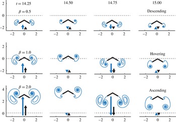
of the background flow oscillations. The flow structures generated by the flyer in these three cases are shown in figure 8. Taken together, figures 7 and 8 show the dependence on
 $\unicode[STIX]{x1D6FD}$
for fixed
 $\unicode[STIX]{x1D6FC}$
,
 $\unicode[STIX]{x1D705}$
and
 $m$
. A systematic study of the dependence on these parameters is discussed next.
Snapshots of the vortex structures of descending, hovering and ascending
 $\unicode[STIX]{x039B}$
-flyer for
 $\unicode[STIX]{x1D6FD}=0.5,1,2$
, respectively. In all three cases, the parameter values are:
 $m=8$
,
 $\unicode[STIX]{x1D6FC}=60^{\circ }$
,
 $\unicode[STIX]{x1D705}=4$
and
 $T_{diss}=0.7T$
. The dashed line marks the starting position of the flyer.

We systematically examine the flyer’s response – namely, descending, hovering, or ascending – as a function of the dimensionless parameters
 $\unicode[STIX]{x1D6FC}$
,
 $m$
,
 $\unicode[STIX]{x1D6FD}$
and
 $\unicode[STIX]{x1D705}$
. To quantify the flyer’s response, we use the change in the
 $T$
-averaged vertical position of the flyer,
 $\unicode[STIX]{x0394}\langle y_{c}\rangle =(\langle y_{c}\rangle |_{t_{2}}-\langle y_{c}\rangle |_{t_{1}})/(t_{2}-t_{1})$
, normalized by the amplitude of the oscillation of the background flow, namely,
 $\unicode[STIX]{x0394}\langle y_{c}\rangle /\unicode[STIX]{x1D6FD}$
. In figure 9, we choose
 $t_{1}=10T$
and
 $t_{2}=20T$
. This choice of
 $t_{1}$
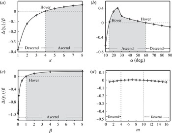
ensures that the flyer has reached its long-term behaviour. Figure 9(b) shows that, for
 $m=8$
,
 $\unicode[STIX]{x1D6FD}=1$
and
 $\unicode[STIX]{x1D705}=4$
, as
 $\unicode[STIX]{x1D6FC}$
increases, the value of
 $\unicode[STIX]{x0394}\langle y_{c}\rangle /\unicode[STIX]{x1D6FD}$
increases, reaches a maximum value, then decreases. Basically, one has two opening angles
 $\unicode[STIX]{x1D6FC}$
for which the flyer hovers in place. For all other values, the flyer either ascends or descends, as indicated. Figure 9(c) shows the flyer’s response as a function of
 $\unicode[STIX]{x1D6FD}$
for
 $\unicode[STIX]{x1D6FC}=60^{\circ }$
,
 $m=8$
and
 $\unicode[STIX]{x1D705}=4$
. Here,
 $\unicode[STIX]{x0394}\langle y_{c}\rangle /\unicode[STIX]{x1D6FD}$
increases with
 $\unicode[STIX]{x1D6FD}$
and reaches a plateau, indicating little or no further increase in the ascension height for larger
 $\unicode[STIX]{x1D6FD}$
. Similarly, figure 9(a) shows that, for
 $\unicode[STIX]{x1D6FC}=60^{\circ }$
,
 $m=8$
and
 $\unicode[STIX]{x1D6FD}=1$
, as the flow acceleration
 $\unicode[STIX]{x1D705}$
increases, the ascension height also reaches a plateau beyond which a further increase in
 $\unicode[STIX]{x1D705}$
only induces a small increase in
 $\unicode[STIX]{x0394}\langle y_{c}\rangle /\unicode[STIX]{x1D6FD}$
. Figure 9(d) examines the flyer’s response as a function of its mass
 $m$
for
 $\unicode[STIX]{x1D6FC}=60^{\circ }$
,
 $\unicode[STIX]{x1D6FD}=1$
and
 $\unicode[STIX]{x1D705}=4$
. Clearly, the flyer’s response is less sensitive to changes in mass than to changes in the other parameters. But note that, for small
 $m$
,
 $\unicode[STIX]{x0394}\langle y_{c}\rangle /\unicode[STIX]{x1D6FD}$
increases slightly as mass increases. This behaviour is intriguing and at first glance seems contrary to physical intuition. However, upon closer examination, we found that at these small values of
 $m$
, the strength of the shed vortices increases as
 $m$
is increased, and that the flyer is mostly entrained by these vortices – thus explaining why, for small
 $m$
, the flyer tends to slightly ascend. As
 $m$
increases further,
 $\unicode[STIX]{x0394}\langle y_{c}\rangle /\unicode[STIX]{x1D6FD}$
levels off at its hovering value, then begin to decrease gently and monotonically. In other words, for larger
 $m$
, heavier flyers descend, consistent with physical intuition.
Flyer’s response as a function of (a) flow acceleration
 $\unicode[STIX]{x1D705}$
, (b) opening angle
 $\unicode[STIX]{x1D6FC}$
, (c) flow amplitude or ‘wing’ size
 $\unicode[STIX]{x1D6FD}$
, and (d) dimensionless mass
 $m$
. Nominal parameter values are:
 $m=8$
,
 $\unicode[STIX]{x1D6FC}=60^{\circ }$
,
 $\unicode[STIX]{x1D6FD}=1$
and
 $\unicode[STIX]{x1D705}=4$
. ‘
 $\diamond$
’ signs represent the numerical data points.

We now examine the parameter values that lead to hovering, i.e.,
 $\unicode[STIX]{x0394}\langle y_{c}\rangle /\unicode[STIX]{x1D6FD}=0$
, as follows. For given values of
 $\unicode[STIX]{x1D6FC}$
,
 $\unicode[STIX]{x1D6FD}$
and
 $m$
, we find the value of the flow acceleration
 $\unicode[STIX]{x1D705}$
at which hovering occurs. This value is unique (figure 9
c) except as function of mass (figure 9
d), in which case we choose the smaller of the two values. Figure 10 shows the dependence of
 $\unicode[STIX]{x1D705}$
on
 $\unicode[STIX]{x1D6FC}$
,
 $\unicode[STIX]{x1D6FD}$
and
 $m$
. We interpret
 $\unicode[STIX]{x1D705}$
as a measure of the aerodynamic effort needed to keep the flyer aloft, as done in Huang et al. (Reference Huang, Nitsche and Kanso2015). This interpretation is consistent with the robotics literature, where the magnitude of the control force is commonly used as a measure of the required control effort. Here, we view flow acceleration
 $\unicode[STIX]{x1D705}$
as a measure of the control effort required to hover. We compare our results to data available from the experiments of Weathers et al. (Reference Weathers, Folie, Liu, Childress and Zhang2010).
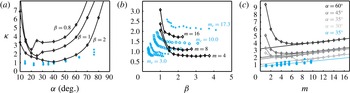
In figure 10(a), we fix
 $m$
and
 $\unicode[STIX]{x1D6FD}$
and vary the opening angle
 $\unicode[STIX]{x1D6FC}$
from
 $10^{\circ }$
to
 $90^{\circ }$
by increments of
 $5^{\circ }$
to
 $10^{\circ }$
. For each value of
 $\unicode[STIX]{x1D6FC}$
, we compute the dimensionless flow acceleration
 $\unicode[STIX]{x1D705}$
for which
 $\unicode[STIX]{x0394}\langle y_{c}\rangle /\unicode[STIX]{x1D6FD}=0$
. The results are depicted in solid black curves. Each curve represents a family of flyers for which the flow amplitude to wing size ratio
 $\unicode[STIX]{x1D6FD}=A/l$
is held constant. Each hovering curve admits a global minimum, that is, for each
 $\unicode[STIX]{x1D6FD}$
, there exists an optimal shape
 $\unicode[STIX]{x1D6FC}$
for which the effort
 $\unicode[STIX]{x1D705}$
required to hover is minimum. Flyers with larger
 $\unicode[STIX]{x1D6FD}$
– that is to say, flyers with smaller wing size or larger flow amplitude – require less effort to hover.
In figure 10(b), we fix the opening angle at
 $\unicode[STIX]{x1D6FC}=35^{\circ }$
, as in Weathers et al. (Reference Weathers, Folie, Liu, Childress and Zhang2010), and vary
 $\unicode[STIX]{x1D6FD}$
by increments equal to one. For each value of
 $\unicode[STIX]{x1D6FD}$
, we compute
 $\unicode[STIX]{x1D705}$
for which
 $\unicode[STIX]{x0394}\langle y_{c}\rangle /\unicode[STIX]{x1D6FD}=0$
. The results are depicted in solid black curves in the parameter space
 $(\unicode[STIX]{x1D6FD},\unicode[STIX]{x1D705})$
in figure 10(b). The numerical hovering conditions are computed for three different flyers of mass
 $m=4,8$
and
 $16$
. Heavier flyers require larger flow acceleration
 $\unicode[STIX]{x1D705}$
. For a flyer of constant mass, a smaller
 $\unicode[STIX]{x1D6FD}$
, which corresponds to either smaller oscillation amplitude
 $A$
or larger wing size
 $l$
, requires a higher flow acceleration
 $\unicode[STIX]{x1D705}$
. As
 $\unicode[STIX]{x1D6FD}$
increases, the effort
 $\unicode[STIX]{x1D705}$
required to hover decreases and seems to reach a plateau beyond which a further change in the amplitude of the flow oscillations or the size of the flyer leads to little or no reduction in the required effort
 $\unicode[STIX]{x1D705}$
.
In figure 10(c), we fix
 $\unicode[STIX]{x1D6FD}=1$
and let the mass of the flyer vary from
 $m=1$
to
 $m=16$
by increments of
 $1$
. For each value of
 $m$
, we compute the minimum value of
 $\unicode[STIX]{x1D705}$
required to hover. The hovering conditions are obtained for four opening angles
 $\unicode[STIX]{x1D6FC}=30^{\circ },35^{\circ },45^{\circ }$
and
 $60^{\circ }$
. Note that, for small values of
 $m$
, the value of
 $\unicode[STIX]{x1D705}$
needed to hover decreases with increasing
 $m$
. This observation is consistent with figure 9(d) but inconsistent with the small mass limit of Weathers et al. (Reference Weathers, Folie, Liu, Childress and Zhang2010), which shows linear dependence of
 $\unicode[STIX]{x1D705}$
on
 $m$
. For larger values of
 $m$
,
 $\unicode[STIX]{x1D705}$
increases linearly with
 $m$
, at a rate that is independent of the flyer’s shape, consistent with the findings of Weathers et al. (Reference Weathers, Folie, Liu, Childress and Zhang2010).
Comparison of numerical results to experimental data from Weathers et al. (Reference Weathers, Folie, Liu, Childress and Zhang2010, figures 2, 5a and 6): (a)
 $\unicode[STIX]{x1D705}$
versus
 $\unicode[STIX]{x1D6FC}$
. Numerical results are shown for various
 $\unicode[STIX]{x1D6FD}$
but the experimental data correspond to one value of
 $\unicode[STIX]{x1D6FD}$
. (b)
 $\unicode[STIX]{x1D705}$
versus
 $\unicode[STIX]{x1D6FD}$
. (c)
 $\unicode[STIX]{x1D705}$
versus
 $m$
. Numerical results are depicted in solid black lines. Experimental data are shown in ‘
 $+$
’, ‘○’, ‘▫’, ‘
 $\times$
’ and ‘▵’, for
 $m_{e}^{+}=17.3$
,
 $m_{e}^{\bigcirc }=10.0$
,
 $m_{e}^{\Box }=6.3$
,
 $m_{e}^{\times }=4.2$
and
 $m_{e}^{\triangle }=3.0$
.

We compare our numerical results to the experimental data of Weathers et al. (Reference Weathers, Folie, Liu, Childress and Zhang2010), where the authors consider a paper pyramid of mass
 $M_{e}$
in flows oscillating at velocity
 $U_{e}=A_{e}(\unicode[STIX]{x03C0}f_{e})\sin (2\unicode[STIX]{x03C0}f_{e}\,t)$
; see figure 1(a). Here we added the subscript
 $e$
to distinguish the experimental conditions from our numerical values. The dependence of the air speed
 $f_{e}A_{e}$
required for hovering on the geometry of a paper pyramid is explored in Weathers et al. (Reference Weathers, Folie, Liu, Childress and Zhang2010, figure 6). The pyramid’s mass is fixed at
 $M_{e}=0.224~\text{g}$
, but its side length
 $l_{e}$
and apex angle
 $\unicode[STIX]{x1D6FC}_{e}$
are varied simultaneously such that
 $W_{e}=2l_{e}\sin \unicode[STIX]{x1D6FC}_{e}=3.5~\text{cm}$
is held constant. For each geometry, four distinct frequencies
 $f_{e}$
are considered. Here, we extract the dimensional values from Weathers et al. (Reference Weathers, Folie, Liu, Childress and Zhang2010, figure 6) and use (2.2) to construct the corresponding dimensionless parameters. Note that by designing the experiments to maintain
 $W_{e}$
constant,
 $\unicode[STIX]{x1D6FC}_{e}$
and
 $\unicode[STIX]{x1D6FD}_{e}$
are not independent. Notwithstanding, we superimpose the experimental values of
 $\unicode[STIX]{x1D6FC}_{e}$
and
 $\unicode[STIX]{x1D705}_{e}$
on figure 10(a). For each
 $\unicode[STIX]{x1D6FC}_{e}$
, the experimental data corresponding to the four distinct frequencies
 $f_{e}$
collapse onto one value for
 $\unicode[STIX]{x1D705}_{e}$
, emphasizing the importance of the dimensionless analysis in identifying the main parameters controlling hovering – in this case, the aerodynamic effort
 $\unicode[STIX]{x1D705}$
.
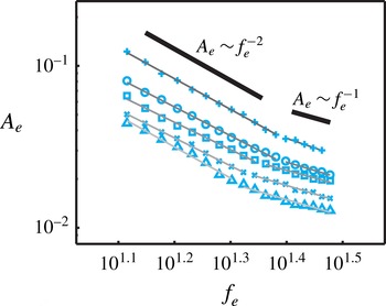
Hovering conditions for flyers of fixed mass and shape. The scaling law is based on the experimental data of Weathers et al. (Reference Weathers, Folie, Liu, Childress and Zhang2010, figure 2) of the peak-to-peak amplitude
 $A_{e}$
(m) versus oscillation frequency
 $f_{e}$
(Hz) plotted on log–log scale.

In Weathers et al. (Reference Weathers, Folie, Liu, Childress and Zhang2010, figure 2) is a depiction of the air speed
 $f_{e}A_{e}$
required for the pyramid-shaped body to hover at a frequency
 $f_{e}$
for various flyer length
 $l_{e}$
. We define the dimensionless mass of the pyramid as
 $m_{e}=M_{e}/\unicode[STIX]{x1D70C}_{f}W_{e}^{3}$
, where
 $M_{e}=0.215$
grams. We map these experimental data onto the parameter space
 $(\unicode[STIX]{x1D6FD},\unicode[STIX]{x1D705})$
as depicted in figure 10(b). The symbols ‘
 $+$
’, ‘○’, ‘
 $\Box$
’, ‘
 $\times$
’ and ‘
 $\triangle$
’ correspond to the experimental results of flyers of different size
 $l_{e}$
and hence different dimensionless mass
 $m_{e}$
. Weathers et al. (Reference Weathers, Folie, Liu, Childress and Zhang2010, figure 5a) shows the dependence of the required air speed
 $f_{e}A_{e}$
for hovering on the mass
 $m_{e}$
of the flyer. We map these data points onto the dimensionless parameter space
 $(m,\unicode[STIX]{x1D705})$
in figure 10(c). The experimental data are shown in filled ‘○’. We find the experimental data collapse onto a straight line, indicating that the flow acceleration
 $\unicode[STIX]{x1D705}_{e}$
depends linearly on
 $m_{e}$
. This is consistent with the simulation results, albeit for larger
 $m$
.
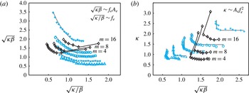
Hovering conditions in terms of (a) dimensionless flow speed
 $\sqrt{\unicode[STIX]{x1D705}\unicode[STIX]{x1D6FD}}=f_{e}A_{e}/\sqrt{gl_{e}}$
and frequency
 $\sqrt{\unicode[STIX]{x1D705}/\unicode[STIX]{x1D6FD}}=f_{e}/\sqrt{l_{e}/g}$
and (b) the dimensionless flow acceleration
 $\unicode[STIX]{x1D705}=A_{e}\,f_{e}^{2}/g$
and flow speed
 $\sqrt{\unicode[STIX]{x1D705}\unicode[STIX]{x1D6FD}}$
. The experimental data from Weathers et al. (Reference Weathers, Folie, Liu, Childress and Zhang2010, figure 2) as well as the numerical results from figure 10(b) show similar trend, namely, for relatively low flow frequencies, or equivalently, large flow speeds, the effort required to hover is constant.

Hovering conditions and scaling law
 $A_{e}\sim f_{e}^{-n}$
based on the experimental data of Weathers et al. (Reference Weathers, Folie, Liu, Childress and Zhang2010, figure 2): the value of
 $n$
is computed using the least square method. For each flyer, the flow amplitude scales as
 $A_{e}\sim f_{e}^{-2}$
for
 $f_{e}<20~\text{Hz}$
and
 $A_{e}\sim f_{e}^{-1}$
for
 $f_{e}>20~\text{Hz}$
. That is, for each flyer, the dimensionless flow acceleration
 $\unicode[STIX]{x1D705}=A_{e}\,f_{e}^{2}/g$
required to hover is constant for
 $f_{e}<20~\text{Hz}$
, whereas the dimensionless flow speed
 $\sqrt{\unicode[STIX]{x1D705}\unicode[STIX]{x1D6FD}}=f_{e}A_{e}/\sqrt{gl_{e}}$
is constant for
 $f_{e}>20~\text{Hz}$
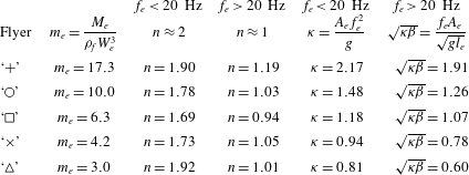
.

In figure 10, the experimental data and numerical results follow similar trends. The general agreement between the model and the experimental data is remarkable given the inherent differences between the three-dimensional pyramid and our two-dimensional flyer, where the fluid–structure interactions are accounted for using the vortex sheet model and the effects of fluid viscosity are approximated using
 $T_{diss}$
. This agreement serves to validate the model, but, most importantly, it offers novel insights into the experimental results, as discussed next.
We map the data from Weathers et al. (Reference Weathers, Folie, Liu, Childress and Zhang2010, figure 2) onto the parameter space (
 $f_{e},A_{e}$
) using a log–log plot in figure 11. We then fit the data into
 $A_{e}\sim f_{e}^{-n}$
using the least square method. The corresponding values of
 $n$
are shown in table 1. For each flyer, at frequencies
 $f_{e}$
less than
 $20~\text{Hz}$
,
 $A_{e}$
scales as
 $f_{e}^{-2}$
while for
 $f_{e}>20~\text{Hz}$
,
 $A_{e}$
scales as
 $f_{e}^{-1}$
. In other words, for each flyer with fixed shape and weight, the flow acceleration
 $A_{e}\,f_{e}^{2}/g$
required to hover is constant at low frequencies, while the air speed
 $f_{e}A_{e}$
is constant at large frequencies.
To emphasize these observations, we map the values of
 $f_{e}$
and
 $f_{e}A_{e}$
onto the dimensionless frequency
 $\sqrt{\unicode[STIX]{x1D705}/\unicode[STIX]{x1D6FD}}$
and dimensionless fluid velocity
 $\sqrt{\unicode[STIX]{x1D705}\unicode[STIX]{x1D6FD}}$
; see figure 12(a). Note the equivalence between the dimensionless and dimensional quantities,
 $\sqrt{\unicode[STIX]{x1D705}/\unicode[STIX]{x1D6FD}}=f_{e}/\sqrt{l_{e}/g}$
and
 $\sqrt{\unicode[STIX]{x1D705}\unicode[STIX]{x1D6FD}}=f_{e}A_{e}/\sqrt{gl_{e}}$
. We observe that, for small oscillation frequency
 $\sqrt{\unicode[STIX]{x1D705}/\unicode[STIX]{x1D6FD}}$
, the speed
 $\sqrt{\unicode[STIX]{x1D705}\unicode[STIX]{x1D6FD}}$
required to hover changes such that their product
 $\unicode[STIX]{x1D705}$
remains constant. For larger frequencies, the amplitude of the flow velocity
 $\sqrt{\unicode[STIX]{x1D705}\unicode[STIX]{x1D6FD}}$
is constant. The values of these constants are indicated in table 1.
Finally, we examine the parameter space of dimensionless flow speed and effort (
 $\sqrt{\unicode[STIX]{x1D705}\unicode[STIX]{x1D6FD}},\unicode[STIX]{x1D705}$
) in figure 12(b). We depict both the experimental data from Weathers et al. (Reference Weathers, Folie, Liu, Childress and Zhang2010, figure 2) and the numerical results from figure 10(b). Interestingly, in both the experimental data and numerical results, for each flyer, at relatively high flow speeds
 $\sqrt{\unicode[STIX]{x1D705}\unicode[STIX]{x1D6FD}}$
, equivalently low flow frequencies
 $\sqrt{\unicode[STIX]{x1D705}/\unicode[STIX]{x1D6FD}}$
, hovering occurs at a constant
 $\unicode[STIX]{x1D705}$
independently of the flow speed
 $\sqrt{\unicode[STIX]{x1D705}\unicode[STIX]{x1D6FD}}$
or frequency
 $\sqrt{\unicode[STIX]{x1D705}/\unicode[STIX]{x1D6FD}}$
.
Taken together, the results in figures 11 and 12 indicate that a given flyer of fixed mass and shape requires either a constant flow speed or a constant flow acceleration (effort) to hover. In particular, at flow frequencies
 $\sqrt{\unicode[STIX]{x1D705}/\unicode[STIX]{x1D6FD}}$
smaller than
 ${\sim}$
1, the flow frequency and speed required to hover must satisfy
 $\unicode[STIX]{x1D705}=$
constant (figure 12(a) and table 1). Meanwhile, at flow frequencies larger than
 ${\sim}$
1, the flow speed
 $\sqrt{\unicode[STIX]{x1D705}\unicode[STIX]{x1D6FD}}$
required to hover is constant. This observation implies that, depending on the value of
 $\sqrt{\unicode[STIX]{x1D705}/\unicode[STIX]{x1D6FD}}$
, there are two hovering regimes: one where a given flyer requires a constant flow acceleration to hover and another where it requires constant flow speed. Further, it is clear from figure 12(b) that at large flow speeds
 $\sqrt{\unicode[STIX]{x1D705}\unicode[STIX]{x1D6FD}}$
, the value of
 $\unicode[STIX]{x1D705}$
required to hover is independent of the flow speed. In other words, at low flow frequencies or, equivalently, large flow speeds, the flow acceleration required to hover depends on the flyer itself, and not on the frequency and amplitude of the flow oscillations.
4 Discussion
A pyramid-shaped rigid object is reported to hover passively in an oscillating background air flow in Weathers et al. (Reference Weathers, Folie, Liu, Childress and Zhang2010). The geometric asymmetry of the object and the unsteady flow structures it produces are responsible for the production of the lift forces necessary to keep it aloft. Here, we presented a model system consisting of a two-dimensional,
 $\unicode[STIX]{x039B}$
-flyer in oscillatory flows, and we studied the two-way coupling between the flyer’s motion and the surrounding fluid in the context of the vortex sheet model. Our results show that the
 $\unicode[STIX]{x039B}$
-flyer hovers in place or descends/ascends depending on its mass and geometric properties as well as on the frequency and amplitude of the oscillatory background flow. The hovering motion is associated with the shedding of vortex dipoles from the flyer’s two outer edges, resulting in a downward momentum flux, as noted qualitatively in Weathers et al. (Reference Weathers, Folie, Liu, Childress and Zhang2010), Liu et al. (Reference Liu, Ristroph, Weathers, Childress and Zhang2012). Although the system studied here does not have a direct biological analogue, the dipolar structures and resulting lift forces observed here are reminiscent of those produced by actively flapping bodies; see, e.g., Ellington (Reference Ellington1984), Warrick, Tobalske & Powers (Reference Warrick, Tobalske and Powers2005).
We examined the response of the
 $\unicode[STIX]{x039B}$
-flyer as a function of the flyer and flow parameters. One has seven dimensional parameters: the gravitational constant
 $g$
, the opening angle
 $\unicode[STIX]{x1D6FC}$
, wing length
 $l$
and mass
 $M$
of the flyer, and the frequency
 $f$
, oscillation amplitude
 $A$
, and density
 $\unicode[STIX]{x1D70C}_{f}$
of the background flow. Following Liu et al. (Reference Liu, Ristroph, Weathers, Childress and Zhang2012), we used non-dimensional analysis to reduce these seven dimensional quantities to four dimensionless parameters: the opening angle
 $\unicode[STIX]{x1D6FC}$
, the mass
 $m$
of the flyer normalized by the fluid density and flyer size, the amplitude of the background oscillations relative to the ‘wing’ length of the flyer
 $\unicode[STIX]{x1D6FD}=A/l$
, and the flow acceleration relative to the gravitational acceleration
 $\unicode[STIX]{x1D705}=Af^{2}/g$
. We interpreted the flow acceleration
 $\unicode[STIX]{x1D705}$
as the aerodynamic effort needed to keep the flyer aloft. We showed that, for flyers of constant
 $\unicode[STIX]{x1D6FD}$
, there exists an optimal opening angle
 $\unicode[STIX]{x1D6FC}$
for which the aerodynamic effort needed to hover is minimum. We then showed that, for flyers of constant mass
 $m$
, when
 $\unicode[STIX]{x1D6FD}$
increases, that is, when the amplitude of flow oscillations increases or the flyer’s size decreases, the flow acceleration
 $\unicode[STIX]{x1D705}$
needed to hover decreases. Lastly, we showed that, for sufficiently heavy flyers, the flow acceleration required to hover depends linearly on the flyer’s mass
 $m$
. The proportionality constant between
 $\unicode[STIX]{x1D705}$
and
 $m$
is independent of the flyer’s opening angle
 $\unicode[STIX]{x1D6FC}$
.
The parameter
 $\unicode[STIX]{x1D6FD}$
admits an alternative interpretation as the ratio of aerodynamic drag to added mass forces. Indeed, steady drag forces scale as
 $(Af)^{2}$
while unsteady added mass scales as
 $l(Af^{2})$
, thus
 $(Af)^{2}/l(Af^{2})=A/l=\unicode[STIX]{x1D6FD}$
. Our result – that the flow acceleration
 $\unicode[STIX]{x1D705}$
needed to hover decreases when
 $\unicode[STIX]{x1D6FD}$
increases – reinforces the dominant effect of the drag forces over the added mass forces in the hovering dynamics. A quasisteady theory based upon drag forces alone was used in Weathers et al. (Reference Weathers, Folie, Liu, Childress and Zhang2010) to successfully estimate the qualitative effect of the shape asymmetry on the hovering motion, albeit it systematically underestimated the lift produced. An unsteady theory based upon added mass effects alone cannot explain the hovering dynamics, since the added mass is invariant under flow reversal (Kanso Reference Kanso2009), and independent of up–down asymmetry. In essence, neither the steady drag forces alone nor the unsteady added mass effect alone are sufficient to predict the unsteady lift force, which is a result of these effects and the effects of the unsteady vortex structures combined.
We compared our hovering results to the experimental results of Weathers et al. (Reference Weathers, Folie, Liu, Childress and Zhang2010, figure 2). Both numerical and experimental results admit the same dependence of
 $\unicode[STIX]{x1D705}$
on
 $\unicode[STIX]{x1D6FD}$
. The agreement of the model with the experimental data is remarkable given the inherent differences between the three-dimensional pyramid and the two-dimensional flyer. The differences also stem from the use of the idealized vortex sheet model and from emulating the effect of fluid viscosity by dissipating the incremental point vortices forming the vortex sheet after a time
 $T_{diss}$
from being shed into the flow. We chose
 $T_{diss}=0.7$
because a close look at Liu et al. (Reference Liu, Ristroph, Weathers, Childress and Zhang2012, figure 2) suggests that the time scale of vorticity dissipation is close to one oscillation period. The effect of
 $T_{diss}$
was examined in Huang et al. (Reference Huang, Nitsche and Kanso2015, figure 3b), where we showed how the numerical results depended on
 $T_{diss}$
. In particular, we showed that as
 $T_{diss}$
increases from
 $0.6$
to
 $0.9$
(viscosity decreases), the hovering results from the numerical study converge towards the experimental results. The interested reader is referred to Huang et al. (Reference Huang, Nitsche and Kanso2015, figure 3b) for a quantitative assessment of the effect of
 $T_{diss}$
.
An important outcome of the comparison between the numerical and experimental data is that, under certain conditions of the flow frequency, namely for frequencies below
 $20~\text{Hz}$
, the flow acceleration required to hover is an intrinsic property of the flyer itself: a given flyer of fixed mass and shape requires a constant
 $\unicode[STIX]{x1D705}$
to hover, irrespective of variations in the frequency
 $f$
and speed
 $fA$
of the oscillating flow. This physical insight may lead to significant implications on understanding active hovering by live organisms that can manipulate their flapping motion to favour a larger oscillation amplitude or frequency, as well as on the bio-inspired design of unmanned air vehicles. We note here that birds typically flap their wings at frequencies below 10 Hz (Pennycuick Reference Pennycuick1990), but larger frequencies (up to 80 Hz or higher) have been recorded in the wingbeat of hummingbirds. Also, insects have wingbeat frequencies ranging from 10 Hz to 1000 Hz (Wang Reference Wang2005). An interesting future study would be to extend the model presented here to flapping flyers and analyse the effect of the flapping frequency and amplitude on hovering.
We conclude by noting that our modelling framework, in addition to its utility in determining the hovering conditions and extracting quantitative design rules for hovering in oscillatory flows, is beneficial for studying the stability of these flyers. A remarkable feature of the hovering pyramid in the experiments of Weathers et al. (Reference Weathers, Folie, Liu, Childress and Zhang2010), Liu et al. (Reference Liu, Ristroph, Weathers, Childress and Zhang2012) is its passive stability and robustness to flow perturbations. Liu et al. (Reference Liu, Ristroph, Weathers, Childress and Zhang2012) uses clever arguments and simplifying approximations to obtain ‘educated guesses’ of the stabilizing mechanism without ever solving the coupled flow–structure interactions. We employed the
 $\unicode[STIX]{x039B}$
-flyer model presented here in Huang et al. (Reference Huang, Nitsche and Kanso2015) to analyse the transition from stable to unstable, yet more manoeuvrable, hovering, as a function of the opening angle
 $\unicode[STIX]{x1D6FC}$
and flow acceleration
 $\unicode[STIX]{x1D705}$
. We found that the transition from passively unstable to passively stable hovering occurs at a post-optimal opening angle, i.e., opening angles for which the flow acceleration
 $\unicode[STIX]{x1D705}$
is not minimum. Future extension of this work will include more detailed analysis of how stability is influenced by the flyer’s size and mass.