1. Introduction
Vortex-induced vibration (VIV) of long flexible structures has been the subject of extensive research in ocean engineering applications such as marine risers and umbilical cables (Bearman Reference Bearman1984; Resvanis & Vandiver Reference Resvanis and Vandiver2022; Huera-Huarte Reference Huera-Huarte2025), in civil engineering applications such as large-span bridges (Ge, Zhao & Cao Reference Ge, Zhao and Cao2022), and more recently in renewable energy structures including wind turbine blades (Grinderslev et al. Reference Grinderslev, Nørmark Sørensen, Raimund Pirrung and González Horcas2022; Fu et al. Reference Fu, Vijayakumar, Lee and Sprague2026) and towers (Livanos Reference Livanos2018).
Flexible pipes present significant challenges for the direct measurement of vortex-induced hydrodynamic force distributions along their length due to continuous deformation and spatially distributed dynamic responses. In contrast, both motion and hydrodynamic force measurements are relatively straightforward for rigid cylinders. As a result, the canonical model for studying the VIV of flexible structures is a circular rigid cylinder placed in a uniform flow (Tian et al. Reference Tian, Zhu, Holmedal, Andersson, Jiang and Pettersen2023), allowed to vibrate freely in both the cross-flow (CF) and in-line (IL) directions (Bearman Reference Bearman1984; Williamson & Govardhan Reference Williamson and Govardhan2004; Han et al. Reference Han, de Langre, Thompson, Hourigan and Zhao2023; Cheng et al. Reference Cheng, Zhang, Wang, Lien and Dowell2024; Benner, Carleton & Modarres-Sadeghi Reference Benner, Carleton and Modarres-Sadeghi2025; Fu et al. Reference Fu, Fu, Han, Niu, Zhang and Zhao2025a ). Key response characteristics such as the vibration amplitude and frequency have been extensively investigated, including phenomena such as lock-in (Gabbai & Benaroya Reference Gabbai and Benaroya2005; Williamson & Govardhan Reference Williamson and Govardhan2008), the critical mass ratio (Govardhan & Williamson Reference Govardhan and Williamson2000) and the Griffin plot (Govardhan & Williamson Reference Govardhan and Williamson2006).
Numerous methods have been proposed to present VIV hydrodynamic forces of the bluff cylinder, among which the approaches developed by Sarpkaya (Reference Sarpkaya1995) and Thorsen, Sævik & Larsen (Reference Thorsen, Sævik and Larsen2017) remain widely adopted. Sarpkaya (Reference Sarpkaya1995, Reference Sarpkaya2004) proposed a VIV force decomposition method consisting of one component in phase with velocity, representing the energy exchange between the fluid and the structure, and another component in phase with acceleration, representing the added mass effect. Thorsen et al. (Reference Thorsen, Sævik and Larsen2017) improved this decomposition by introducing a consistent drag force model that connects the forces in the IL and CF directions. Due to the difficulty of fully exploring the parameter space in traditional freely vibrating experiments, forced vibration tests with prescribed harmonic motion (Gopalkrishnan Reference Gopalkrishnan1993; Aronsen & Larsen Reference Aronsen and Larsen2007; Patel, Rothstein & Modarres-Sadeghi Reference Patel, Rothstein and Modarres-Sadeghi2023) have been conducted to investigate the hydrodynamic characteristics of rigid cylinders undergoing VIV. Comprehensive experiments including CF-only forced motion (Gopalkrishnan Reference Gopalkrishnan1993), IL-only forced motion (Aronsen & Larsen Reference Aronsen and Larsen2007) and IL & CF forced motion (Dahl Reference Dahl2008; Dahl et al. Reference Dahl, Hover, Triantafyllou and Oakley2010; Yin & Larsen Reference Yin and Larsen2011) are conducted to determine the VIV excitation range and excitation coefficient curve.
Slender structures in applications are subjected to a wide variety of flow conditions. The VIV experiments on flexible risers under various flow conditions provide a fundamental understanding of the VIV characteristics of flexible pipes, and serve as a benchmark for numerical analysis. Flexible pipes can be categorised into tension-dominated (Huera-Huarte Reference Huera-Huarte2006; Zheng et al. Reference Zheng, Dahl, Modarres-Sadeghi and Triantafyllou2014a ; Duan et al. Reference Duan, Zhou, You and Wang2021) and bending-stiffness-dominated (Nielsen, Søreide & Kvarme Reference Nielsen, Søreide and Kvarme2002) types, depending on the relative contributions of tension and bending stiffness to their natural frequencies. Tension-dominated flexible pipe VIV is typically more complicated with multi-mode coupled responses (Zheng et al. Reference Zheng, Price, Modarres-Sadeghi and Triantafyllou2014b ). Numerous VIV experiments on flexible risers have been conducted under various flow conditions: uniform flow (Chaplin et al. Reference Chaplin, Bearman, Huera-Huarte and Pattenden2005), linearly sheared flow (Tognarelli et al. Reference Tognarelli, Slocum, Frank and Campbell2004; Trim et al. Reference Trim, Braaten, Lie and Tognarelli2005), three-dimensional flow (Kim et al. Reference Kim, Sævik, Wu and Leira2022) and lake tests (Vandiver et al. Reference Vandiver, Marcollo, Swithenbank and Jhingran2005).
Due to the challenges associated with the direct measurement of VIV hydrodynamic force distributions of the flexible pipe, recent research has focused on estimating these force distributions indirectly through strain or displacement measurements (Wu Reference Wu2011; Song et al. Reference Song, Fu, Cao, Ma and Wu2016a ). For mono-frequency VIV responses, the hydrodynamic behaviour can be accurately characterised using constant excitation and added mass coefficients (Bourguet, Lucor & Triantafyllou Reference Bourguet, Lucor and Triantafyllou2012). Huera-Huarte, Bearman & Chaplin (Reference Huera-Huarte, Bearman and Chaplin2006) were among the first to employ inverse finite element analysis to estimate the hydrodynamic force distribution in a stepped-flow VIV experiment. Song et al. (Reference Song, Fu, Cao, Ma and Wu2016a ) proposed a hydrodynamic force estimation method based on an inverse finite element method in which the hydrodynamic forces were directly estimated using the differential governing equations of a tensioned beam model, and applied for several flexible riser experiments under different flow conditions at Shanghai Jiao Tong University. In addition to the least squares method, Wu (Reference Wu2011) developed a hydrodynamic coefficient identification approach using Kalman filtering and an optimisation-based approach, based on experimental data obtained from tests conducted at the Norwegian Marine Technology Research Institute. These methods have been applied for mono-frequency VIV under uniform flow and linearly sheared flow analysis. However, these studies, which are based on the assumption of constant hydrodynamic coefficients, become inadequate when addressing multi-frequency or modulated VIV responses, where the hydrodynamic forces exhibit strong nonlinearity. To capture the unsteady hydrodynamic behaviour under such conditions, time-varying hydrodynamic coefficients have been introduced (Liu et al. Reference Liu, Fu, Zhang and Ren2018, Reference Liu, Fu, Zhang, Ren and Xu2020; Fu et al. Reference Fu, Fu, Zhang, Han, Ren, Xu and Zhao2022b ), which can accurately capture the hydrodynamics of multi-frequency VIV under shear flow (Liu et al. Reference Liu, Fu, Zhang and Ren2018), and modulated VIV under time-varying oscillatory flow (Liu et al. Reference Liu, Fu, Zhang, Ren and Xu2020; Fu et al. Reference Fu, Fu, Zhang, Han, Ren, Xu and Zhao2022b ). This approach provides a robust framework to demonstrate the time-varying characteristics of multi-frequency and modulated VIV hydrodynamics.
Computational fluid dynamics (CFD) approaches are mainly adopted to investigate the fluid characteristics and fluid–structure interaction behaviour of flexible pipes. For low aspect ratio flexible pipe and bluff cylinder VIV experiments, flow field measurement techniques can be employed to capture the fluid domain (Govardhan & Williamson Reference Govardhan and Williamson2000; Jung et al. Reference Jung, Kim, Park and Lee2018). However, accurately measuring flow characteristics remains challenging, particularly for high aspect ratio flexible pipes VIV. Numerical studies focusing on flexible pipes remain relatively limited due to the complex fluid–structure interactions involving multiple vibration modes and nonlinear wake dynamics. Some simulation results of uniform flow (Evangelinos & Karniadakis Reference Evangelinos and Karniadakis1999; Willden & Graham Reference Willden and Graham2001; Dahl et al. Reference Dahl, Hover, Triantafyllou, Dong and Karniadakis2007; Modarres-Sadeghi et al. Reference Modarres-Sadeghi, Mukundan, Dahl, Hover and Triantafyllou2010; Bourguet et al. Reference Bourguet, Modarres-Sadeghi, Karniadakis and Triantafyllou2011b
, Reference Bourguet, Lucor and Triantafyllou2012; Fan et al. Reference Fan, Wang, Triantafyllou and Karniadakis2019b
; Wang et al. Reference Wang, Fan, Triantafyllou and Karniadakis2021b
), and linearly sheared flow (Bourguet et al. Reference Bourguet, Karniadakis and Triantafyllou2011a
, Reference Bourguet, Lucor and Triantafyllou2012, Reference Bourguet, Karniadakis and Triantafyllou2013) have established fundamental knowledge for flexible pipe VIV. Newman & Karniadakis (Reference Newman and Karniadakis1997) applied direct numerical simulations (DNS) of a
 $4\pi$
long flexible pipe at Reynolds numbers of approximately
 $100$
, revealing the fundamental VIV characteristics such as travelling wave wake patterns. Furthermore, Evangelinos & Karniadakis (Reference Evangelinos and Karniadakis1999) and Bourguet et al. (Reference Bourguet, Karniadakis and Triantafyllou2011a
) conducted DNS to investigate the fundamental characteristics of flexible pipe at Reynolds numbers of approximately
 $1000$
using Nektar++. Willden & Graham (Reference Willden and Graham2004) applied the velocity–vorticity method to simulate flexible pipe VIV at Reynolds numbers of approximately
 $300$
, named VIVIC. Fan et al. (Reference Fan, Wang, Triantafyllou and Karniadakis2019b
) and Wang et al. (Reference Wang, Fan, Triantafyllou and Karniadakis2021b
) applied strip methods to numerically investigate flexible pipe VIV at relatively high Reynolds numbers of approximately
 $2000$
using Nektar++, illustrating the relationships between flexible pipe free vibration and the forced vibration of a bluff cylinder. In the strip method, the flow is treated as a series of two-dimensional sections coupled with a three-dimensional beam model, and few studies have been conducted to improve the method (Bao et al. Reference Bao, Palacios, Graham and Sherwin2016; Deng, Zhao & Wan Reference Deng, Zhao and Wan2020).
For the numerical simulation of VIV of long flexible pipes, the strip method offers a more practical and feasible approach. Recent studies have attempted to connect wake dynamics with hydrodynamic coefficients via simultaneous flow visualisation and structural response measurements. Bourguet et al. (Reference Bourguet, Modarres-Sadeghi, Karniadakis and Triantafyllou2011b ) proposed that the excitation coefficient is related to the vibration phase difference. Fan et al. (Reference Fan, Wang, Triantafyllou and Karniadakis2019b ) and Wang et al. (Reference Wang, Fan and Triantafyllou2021a ) reported that vortex shedding patterns such as 2S (two single vortices), 2P (two pairs of vortices), or P + S (one pair plus one single vortex) are related to the added mass coefficients; a negative added mass coefficient is associated with the P + S and 2P wake patterns. For wake field analysis, spectral proper orthogonal decomposition (SPOD) can be used to extract coherent flow structures in both space and time (Sieber, Paschereit & Oberleithner Reference Sieber, Paschereit and Oberleithner2016; Towne, Schmidt & Colonius Reference Towne, Schmidt and Colonius2018). This ability to identify frequency-dependent flow modes makes SPOD a suitable tool for cylinder wake field analysis. The SPOD has been applied to bluff body wakes (Willert Reference Willert2025; Maleki et al. Reference Maleki, Grace, Mankbadi and Golubev2026) and to the wakes of VIV bluff cylinders undergoing VIV (O’Neill et al. Reference O’Neill, Schubert, Sieber, Martinuzzi and Morton2021) and forced motion (Zhou & Zheng Reference Zhou and Zheng2023).
A unique subsurface flow environment induced by internal waves has been observed in the South China Sea. A six-month field survey conducted in the Liuhua area by the China National Offshore Oil Corporation Research Institute (Xie et al. Reference Xie, Li, Ren and Lei2018) revealed a distinctive shear flow structure characterised by nearly opposite flow directions, asymmetric velocity magnitudes, and a sharp velocity gradient centred around a depth of approximately 185 m. This bidirectionally sheared flow condition was found to occur frequently, resulting in an average exposure of approximately 18.6 hours per month. Besides the South China Sea, similar bidirectionally sheared flow has also been reported in association with internal wave in other ocean regions (Garrett & Munk Reference Garrett and Munk1979; MacKinnon et al. Reference MacKinnon2017), including areas of engineering interest such as the Gulf Stream and continental slope regions. Moreover, such unique flow conditions have been observed beneath ice-covered areas in polar regions, where melting processes contribute to the formation of bidirectionally sheared flow profiles (Jacobs et al. Reference Jacobs, Jenkins, Giulivi and Dutrieux2011; Minowa et al. Reference Minowa, Sugiyama, Ito, Yamane and Aoki2021).
A joint industry project (JIP), Flow-induced Forces and their Effects on Risers and Subsea Structures (FIFERS), has been proposed and established to develop VIV prediction models for complex flow fields, including bidirectionally sheared flow. As a core component of this JIP, Fu et al. (Reference Fu, Fu, Ren, Xie, Xu, Zhang, Liu and Meng2022a ,Reference Fu, Zhang, Fu, Zhao, Ren and Xu c ) first conducted an ocean basin experiment with a flexible pipe under bidirectionally sheared flow, observing multi-frequency responses and distinctive travelling wave patterns. Moreover, Fu et al. (Reference Fu, Fu, Niu, Zhao, Shen and Deng2025b ) developed an open-source code based on the strip method, and simulated the VIV of a flexible pipe under bidirectionally sheared flow, with validation against experimental results. This study primarily focused on comparing the displacement responses of the flexible pipe under different flow conditions, including uniform, linearly sheared and bidirectionally sheared flow cases, whereas detailed analyses of the corresponding hydrodynamic forces were not conducted.
In this paper, we further investigate the hydrodynamic properties of a flexible pipe subjected to bidirectionally sheared flow. Both experimental and numerical analyses are conducted. The experimental investigation is based on a previously published test apparatus (Fu et al. Reference Fu, Fu, Ren, Xie, Xu, Zhang, Liu and Meng2022a
), and the numerical analysis is performed using a validated simulation framework (Fu et al. Reference Fu, Fu, Niu, Zhao, Shen and Deng2025b
). The model has diameter 28.41 mm and the length is
 $269$
times of the diameter. This study aims to investigate the similarities and differences in hydrodynamic coefficients between bidirectionally sheared flow and unidirectional flows. Based on the experimental and numerical simulation results of VIV under bidirectionally sheared flow, four aspects of the VIV hydrodynamic characteristics are investigated: (i) how bidirectionally sheared flow modifies the mean displacement and drag coefficient distributions and the corresponding mean hydrodynamic force; (ii) whether the antisymmetric velocity distribution of the bidirectionally sheared flow affects the phase distribution of the VIV response; (iii) whether the excitation coefficients exhibit symmetry at the flow velocity reversal point; and (iv) the relationship between the added mass coefficient and the wake vortex patterns.
This paper is organised as follows. Section 2 presents the experimental apparatus and set-up, and the numerical method. Section 3 discusses the IL mean drag characteristics, including the mean drag coefficient, shear force and moment, and the influence of the flow velocity distribution. Section 4 presents the hydrodynamic properties of the flexible pipe under bidirectionally sheared flow, including the dominant frequencies, time-varying hydrodynamic behaviour, and corresponding wake pattern. Finally, § 5 summarises the main conclusions of this study.
2. Experimental and numerical methods
2.1. Experimental set-up
The experiment was conducted in an ocean basin at Shanghai Jiao Tong University. The pipe model was fixed at both ends to a circular driven gear under pre-tension 980 N. The flow field was generated by rotating the driven gear via a timing belt powered by a servo motor to generate the inflow conditions, as figure 1 shows. This novel VIV experimental apparatus has been validated through a comprehensive credibility assessment, including analyses of wake effects, vibration duration, mechanical noise, repeatability and water-depth sensitivity, as reported in our previous work (Fu et al. Reference Fu, Fu, Ren, Xie, Xu, Zhang, Liu and Meng2022a ) and summarised in Appendix A.
The coordinate system is defined as
 $O\text{-}XYZ$
, as shown in figures 1 and 2. The origin (
 $O$
) is set at one end of the pipe model connected with a fixing device with no tensioner. The
 $X,Y,Z$
axes correspond to the IL, CF and spanwise directions of the test pipe model, respectively, with the coordinate system rotating together with the pipe during the test. The rotation direction during the experiment is always along the
 $X$
axis, and the effective current profile is shown with colours and arrows in figure 1.
The overview in figure 2(a) highlights the rotation system driven by a servo motor through a timing belt and synchronous wheel, with the flexible pipe model supported along the circular frame and instrumented by the data acquisition (DAQ) system. The rotation direction and the global coordinate system are also indicated in figure 2(a). Furthermore, figures 2(b) and 2(c) provide close-up views of the end-connection assemblies, including the universal joint and clamps that accommodate rotational motion while constraining the pipe, and the tensioner used at the maximum
 $z$
end to maintain the prescribed axial tension and boundary condition. During the experimental test, universal joints were used to implement a pin–pin end condition for the test pipe, and due to the extra tensioner length difference, the velocity at the maximum spanwise location is approximately
 $4.5\,\%$
lower than that at the coordinate origin. During each test, the pipe is rotated through one full cycle, which contains nearly
 $50$
fully developed VIV periods; further details are provided in Appendix A.
The experimental set-up. (a) Diagram of the experimental apparatus. The flow field is generated by rotation of the driven gear with a bidirectionally sheared distribution. (b) The flow velocity profile from the experiment shows that the minimum negative velocity
 $-U_m$
occurs at
 $Z/L = 0$
, and the maximum velocity
 $U_m$
occurs at
 $Z/L = 1$
.

Experimental set-up of the rotating apparatus in the ocean basin testing in air. (a) Overview of the facility. (b) Close-up of the maximum
 $Z$
end connection showing the universal joint, clamp and tensioner. (c) Close-up of the original end connection showing the universal joint and clamp.

The pipe model consists of an external polypropylene random copolymer pipe and an internal copper cable. Silicone rubber is applied between the layers to prevent relative sliding. A total of 46 fibre Bragg grating (FBG) strain sensors, divided into four groups, are installed along the test pipe to measure dynamic strains in both the IL and CF directions, providing 14 measurement points in the IL direction, and 9 measurement points in the CF direction. The LUNA SM130 optical sensing interrogator was used to measure the dynamic strain, with calibration performed prior to the tests. Modal analysis is applied to obtain the VIV displacement, while the details and strain sensor distribution are displayed in Appendix B.
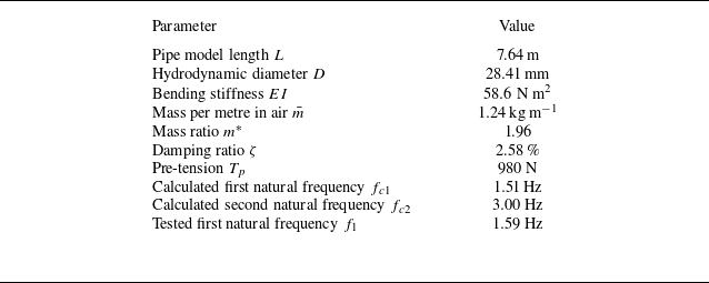
The physical parameters are shown in table 1. The first natural frequency in water is calculated as
 \begin{align} f_{c1}=\frac {\pi }{2} \sqrt {\left (1+\frac {L^{2} T_{p}}{\pi ^{2} E I}\right ) \frac {E I}{\bar {m}^{\prime } L^{4}}},\quad \bar {m}^{\prime }=\bar {m}+\frac {1}{4} C_{m} \rho \pi D^{2}, \end{align}
where
 $C_{m}$
is chosen as
 $1.00$
for the free decay test (Khalak & Williamson Reference Khalak and Williamson1997),
 $\rho = {998}\,\mathrm{kg\,m^{-3}}$
is the density of water in the ocean basin, and
 $\bar {m}$
is mass per metre in air with value in table 1. The tested natural frequency is obtained by a free decay test, which differs by 5 % from the theoretical value.
Values of physical properties of the test pipe model.

The relative Reynolds number
 $ \textit{Re}_r:= UD/\nu$
is the Reynolds number
 $ \textit{Re}$
with respect to the relative flow direction in the spanwise direction, and
 $ \textit{Re}_m:=U_m D/\nu$
is defined as the maximum of the relative Reynolds number
 $ \textit{Re}_r$
, where
 $U_m$
is the maximum velocity shown in figure 1, and
 $\nu ={1\times 10^{-6}}\,\mathrm{m^2\,s^{-1}}$
is the kinematic viscosity of water. The apparatus is driven by a servo motor at a prescribed constant rotational speed to generate the desired flow field. A total of 58 experimental cases are conducted, with maximum flow velocity
 $U_{m}$
varied from
 $0.30$
to
 ${1.39}\,\mathrm{m\,s^{-1}}$
, and maximum Reynolds numbers
 $ \textit{Re}_m$
ranging from 8523 to 39 490 within the subcritical
 $ \textit{Re}$
range (Achenbach Reference Achenbach1971).
2.2. Numerical method
The numerical method is developed based on incompressible flow solver OpenFOAM with strip method expansion. The governing equation of the test pipe follows the tensioned Euler–Bernoulli beam model:
 \begin{align} \textit{EI}\frac {\partial ^4\boldsymbol{\xi }(z,t)}{\partial z^4}-\frac \partial {\partial z}{\left [T\frac {\partial \boldsymbol{\xi }(z,t)}{\partial z}\right ]}+c\frac {\partial \boldsymbol{\xi }(z,t)}{\partial t}+\bar {m}\frac {\partial ^2\boldsymbol{\xi }(z,t)}{\partial t^2}=\boldsymbol{F}(z,t), \end{align}
where
 $\boldsymbol{\xi } = [\xi _x, \xi _y]$
is the vibration displacement in the IL and CF directions,
 $c = 2\bar {m}\omega _d \zeta$
is the structural damping,
 $\omega _d$
is the dominant frequency,
 $T$
is the tension of the pipe, and
 $\boldsymbol{F} = [F_x, F_y]$
is the force in the IL and CF directions. In the numerical configuration, the pipe is fixed in space and is exposed to a prescribed bidirectionally sheared flow profile that is steady in time but varies along the span. Specifically, the local inflow velocity is imposed as a function of the spanwise coordinate, such that both its magnitude and direction change with
 $Z$
to reproduce the equivalent bidirectionally sheared flow profile, as shown in figure 1(b). The simulations aim to avoid the wake effects of the rotating pipe and the difficulty of using a dynamic mesh. For each flow case, the simulation is advanced for approximately
 ${60}\,\mathrm{s}$
of physical time to ensure that the VIV response fully develops. The initial transient stage is discarded, and only the last
 $40\,\%$
of the time record, containing at least
 $20$
vibration periods after the response reaches a statistically steady state, is used for post-processing. A representative VIV development process is shown in Appendix A, and VIV response takes approximately
 $15$
s to reach the fully developed regime.
The force of each strip is obtained using incompressible Navier–Stokes equations solver OpenFOAM. Each strip domain has size
 $20D\times 50D$
, with the cylinder located in the centre of the domain. The boundary conditions are set as symmetry on the top and bottom boundaries, and inlet and outlet on the left- and right-hand boundaries, respectively, which is consistent with Bourguet, Karniadakis & Triantafyllou (Reference Bourguet, Karniadakis and Triantafyllou2013), Fan et al. (Reference Fan, Wang, Triantafyllou and Karniadakis2019b
) and Fu et al. (Reference Fu, Fu, Zhang, Han, Ren, Xu and Zhao2022b
). The flow is solved using the shear stress transport
 $k{-}\omega$
turbulence model with second-order accuracy in both spatial and temporal discretisations, and the time step is constrained by a Courant–Friedrichs–Lewy number less than unity. The force is obtained based on
 \begin{align} \boldsymbol{F}=\oint \left (p\boldsymbol{I}+\mu \boldsymbol{R}_{dev}\right )\boldsymbol{\cdot }\mathrm{d}\boldsymbol{S}, \end{align}
where
 $p$
is the pressure,
 $\boldsymbol{R}_{dev}$
is the deviatoric Reynolds stress tensor (Jasak Reference Jasak1996),
 $\mu$
is the dynamic viscosity of the fluid, and
 $\boldsymbol{S}$
is the face area vector. The weak-coupling algorithm is applied for VIV simulation, where the fluid and structural domains exchange data once per time step. For more details, including the time step and mesh size independence analysis for the simulation framework, refer to Fu et al. (Reference Fu, Fu, Niu, Zhao, Shen and Deng2025b
). Five numerical simulations are performed at maximum Reynolds numbers
 $ \textit{Re}_m$
13 637, 17 330, 21 876, 28 216 and 32 672 in the present study. Both the experimental and numerical results are processed using the same procedures, as described below.
3. Mean drag properties
The VIV response of a flexible pipe consists of three components: (i) the mean displacement in the IL direction induced by the mean drag, (ii) the fluctuating VIV response superimposed on the IL mean displacement with zero mean value, which presents the IL VIV response, and (iii) the fluctuating VIV response in the CF direction with zero mean value (Huera-Huarte Reference Huera-Huarte2006), which presents the CF VIV response. The inverse finite element method (Wu Reference Wu2011) is applied to reconstruct the spanwise distribution of hydrodynamic forces from strain measurements along the pipe. This approach has been adopted in the VIV community to overcome the practical difficulty of directly measuring distributed hydrodynamic forces on a flexible structure (Huera-Huarte Reference Huera-Huarte2025).
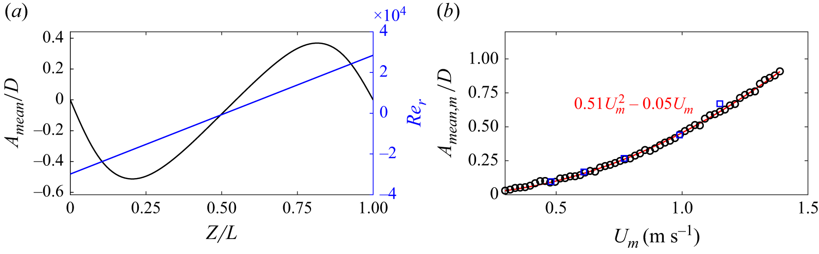
Analysis of experimental results reveals a bidirectional distribution of mean IL displacement induced by the mean drag force, as figure 3(a) shows, which is attributed to the bidirectional characteristics of the flow field. This section introduces the characteristics of the mean drag, shear force and moment, as well as the effects of the flow velocity distribution. In addition, the numerical simulation results are also presented to further strengthen the credibility of the findings.
3.1. Mean displacement and mean drag coefficient
Figure 3 illustrates the mean IL displacement
 $A_{mean}/D$
that is induced by the mean drag, and the corresponding flow velocity distribution characterised by the relative Reynolds number
 $ Re_r$
, for the case associated with
 $U_m = {0.87}\,\rm{m\,s^{-1}}$
, the maximum Reynolds number
 $ \textit{Re}_m = 2.48 \times 10^4$
, and the maximum mean IL displacement
 $A_{\textit{mean},m}/D$
across different test conditions. Here,
 $A_{\textit{mean},m}$
is defined as the spanwise maximum of the magnitude of the local mean IL displacement
 $A_{\textit{mean},m} \equiv \max _{z \in [0,L]} \left |A_{mean}(z)\right |$
. In figure 3(a), the blue curve represents the flow velocity profile, which displays a bidirectional shear pattern. The velocity reaches its minimum value
 $ -U_m$
at
 $ Z = 0$
, and increases linearly towards maximum value approximately
 $U_m$
at
 $ Z = L$
. The black curve denotes the mean IL displacement distribution, which exhibits a sinusoidal shape, consistent with the applied flow condition.
Figure 3(b) presents the polynomial fit of the relationship between the maximum mean displacement
 $A_{\textit{mean},m}$
and the flow velocity. The black circles and blue squares represent the experimental and simulation results of the mean displacement, respectively. The fitted curve adopts a quadratic form with a zero intercept from experimental data, expressed as
 $A_{\textit{mean},m}/D = 0.51U_m^2 - 0.05U_m$
. The fitting indicates that the second-order term dominates the correlation, suggesting a nonlinear dependence of the mean displacement on the inflow velocity magnitude. The blue squares represent the simulation results, which agree well with the experimental data, exhibiting the same second-order trend.
Mean displacement distribution along the pipe and maximum value versus flow velocity. (a) Mean displacement distribution in the IL direction (black line), and relative flow velocity distribution (blue line) at
 $U_m= {0.87}\,{\rm{m\,s^{-1}}}\;(Re_m = 2.48\times 10^4)$
based on experimental data. (b) Maximum mean displacement
 $A_{\textit{mean},m}/D$
versus
 $U_m$
of experiment results (black circles) and simulation results (blue squares), with fitting result based on
 $U_m$
(red line) as
 $A_{\textit{mean},m}/D = 0.51U_m^2-0.05U_m$
.

The mean drag
 $F_{md}(z)$
is the mean value of force in the IL direction in (2.2) as the time average of the drag force as
 $F_{md}(z) = \langle F_x(z,t) \rangle _t$
, and the drag coefficient
 $C_d(z)$
is expressed as
 \begin{align} C_d (z) = \frac {2\,F_{md}(z)}{\rho D\, U(z)\, \lvert U(z) \rvert }, \end{align}
where
 $U(z)$
denotes the local flow velocity at spanwise position
 $z$
. As shown in figure 3, the maximum mean IL displacement is approximately
 $1.0D$
as
 ${28.41}\,\mathrm{mm}$
. Over a segment of length
 $0.25L$
, the corresponding local inclination angle is estimated to be
 $0.84^\circ$
, indicating that its influence on the normal-velocity correction is negligible. Therefore, we use
 $U(z)$
as the reference velocity in (3.1). However, it should be noted that this conclusion is only validated over the Reynolds number range
 $ \textit{Re} \in [{8523},{39\,490}]$
in the present study, and a correction would be required for higher
 $ \textit{Re}$
and larger length-to-diameter ratios.
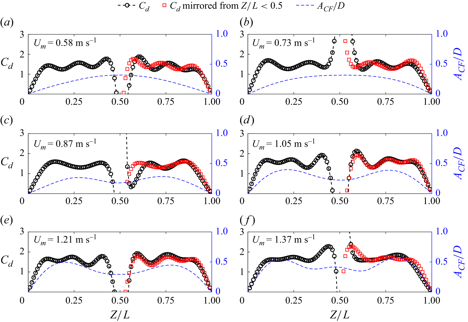
Figure 4 presents the spanwise distribution of the drag coefficient
 $C_d(z)$
for six representative cases with increasing flow velocity
 $U_m = 0.58, 0.73, 0.87, 1.05, 1.21, 1.37$
 $\rm{m\,s^{-1}}$
. Across all cases, the mirrored curves (red squares) closely collapse onto the measurements over most of the span, demonstrating that the spanwise distribution of the mean drag is largely symmetric with respect to the mid-span (
 $Z/L=0.5$
). In particular, both the averaged value and the spatial variation trend of
 $C_d(z)$
are well reproduced by the mirrored profiles, which indicates that the drag coefficient distributions remain consistent when the background velocity direction changes. The mirrored profiles show some small differences from the measurements, mainly occurring in the mid-span velocity direction change region and near the two ends, where our experimental boundary condition set-up, shown in figure 2, can introduce such small asymmetry over the spanwise direction. In flexible pipe VIV studies, analysis typically focuses on a well-behaved spanwise region with consistent response statistics, while portions affected by end boundary conditions and local singularities are excluded, and this practice also reflects the main VIV region of engineering risers (Trim et al. Reference Trim, Braaten, Lie and Tognarelli2005).
Meanwhile, overlaying the spanwise distributions of the VIV response
 $A_{\textit{CF}}/D$
and the drag coefficient
 $C_d$
does not reveal an obvious one-to-one relationship. For example, figures 4(a) and 4(b) show essentially the same CF response shape but different
 $C_d$
distributions, and a similar observation can be made by comparing figures 4(c) and 4(d). In flexible pipe VIV analysis, it is therefore more common to examine relationships based on spanwise-averaged quantities as discussed below.
Drag coefficient
 $C_d$
(black circles with dashed line), mirrored drag coefficient from
 $Z/L\lt 0.5$
(red squares), and non-dimensional root mean square displacement in the CF direction
 $A_{\textit{CF}}/D$
(blue dashed line) of different cases based on experimental data: (a)
 $U_m = {0.58}\,\mathrm{m\,s^{-1}} \; (Re_m = 1.65 \times 10^4)$
, (b)
 $U_m = {0.73}\,\mathrm{m\,s^{-1}} \; (Re_m = 2.07 \times 10^4)$
, (c)
 $U_m = {0.87}\,\mathrm{m\,s^{-1}} \; (Re_m = 2.47 \times 10^4)$
, (d)
 $U_m = {1.05}\,\mathrm{m\,s^{-1}} \; (Re_m = 2.98 \times 10^4)$
, (e)
 $U_m = {1.21}\,\mathrm{m\,s^{-1}} \; (Re_m = 3.44 \times 10^4)$
and (f)
 $U_m = {1.37}\,\mathrm{m\,s^{-1}} \; (Re_m = 3.89 \times 10^4)$
.

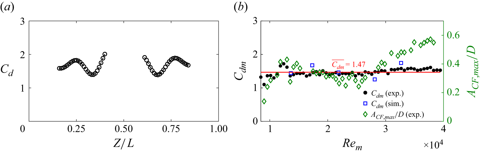
Figure 5(a) presents the spanwise distribution of the drag coefficient
 $C_d$
for the case
 $U_m={1.19}\,\mathrm{m\,s^{-1}}$
. Only the two valid regions (
 $0.1\leqslant Z/L \leqslant 0.4$
and
 $0.6\leqslant Z/L \leqslant 0.9$
) are reported; measurements near the two ends are excluded due to end effects, whereas the central region is omitted because the extremely low local flow velocity yields unrealistically large
 $C_d$
values from (3.1), as shown in figure 4. Within the retained regions,
 $C_d$
fluctuates around its spanwise-averaged value. Moreover, the close agreement between the original and mirrored distributions supports the use of a near-symmetric mean drag assumption in the subsequent analysis.
Drag coefficient
 $C_d$
along the pipe and the mean drag coefficient
 $C_{dm}$
with different
 $ \textit{Re}_m$
cases. (a) Drag coefficient (black circles with dashed line) at
 $U_m = {1.19}\,\mathrm{m\,s^{-1}} \; (Re_m = 3.38 \times 10^4)$
for
 $Z/L \in [0.1,\,0.4] \cup [0.6,\,0.9]$
based on experimental data. (b) Mean drag coefficient versus
 $ \textit{Re}_m$
of experimental results (black circles) and simulation results (blue squares), maximum RMS CF displacement along the spanwise direction from Fu et al. (Reference Fu, Fu, Ren, Xie, Xu, Zhang, Liu and Meng2022a
) (green diamonds) and the mean value of mean drag coefficient of all experimental cases
 $\overline {C_{dm}} = 1.47$
(red line).

Figure 5(b) shows the mean drag coefficient
 $C_{dm}$
, defined as the spanwise-average drag coefficient
 $C_{dm}=\langle C_d(z)\rangle _Z$
, which is averaged over the selected spanwise regions shown in figure 5(a). The values of
 $C_{dm}$
remain nearly constant across cases with different Reynolds numbers
 $ \textit{Re}_m$
. To quantify this trend, we further compute the average value over all
 $N$
test conditions within
 $ \textit{Re}_m\in [8523,{39\,490}]$
in figure 5(b) as
 $ \overline {C_{dm}}=({1}/{N})\sum _{n=1}^{N} C_{dm}^{(n)}$
, where
 $C_{dm}^{(n)}$
denotes the mean drag coefficient of the
 $n$
th test condition. Here, we obtain
 $\overline {C_{dm}}=1.47$
for the present study based on experimental data as shown in figure 5(b). The blue squares denote simulation results processed using the same procedure as the experimental data stated above, and show good agreement with the measurements.
We further investigate the relation between the drag coefficient and the VIV displacement magnitude by plotting the maximum root mean square (RMS) CF displacement amplitude along the spanwise direction
 $A_{\textit{CF},\textit{max}}/D$
in figure 5(b). Here, figure 5(b) shows that the mean drag coefficient of a flexible pipe under bidirectionally sheared flow exhibits limited sensitivity to changes in
 $ \textit{Re}_m$
, even though the VIV response amplitude in the CF direction displays an amplitude jump phenomenon when increasing
 $ \textit{Re}_m$
. This suggests that there is no clear relationship between the mean drag coefficient and VIV amplitude subject to bidirectionally sheared flow. This behaviour differs from that observed in uniform flow, where the span-averaged drag coefficient
 $C_{dm}$
is generally found to be strongly correlated with the CF vibration amplitude. For example, Vandiver (Reference Vandiver1983) proposed the empirical relation
 $C_{dm}= C_{d0} [1 + 1.043 (2A_{\textit{CF},\textit{max}}/D)^{0.65}]$
, and Jhingran, Jaiswal & Vandiver (Reference Jhingran, Jaiswal and Vandiver2008) subsequently extended this approach to sectional drag coefficients as
 $C_{d}(z)= C_{d0} [1 + 1.043 (2A_{\textit{CF}}(z)/D)^{0.65}]$
, where
 $C_{d0}$
is the stationary bluff cylinder drag coefficient under the same
 $ \textit{Re}$
. However, in bidirectionally sheared flow VIV, we found that the mean drag coefficient
 $C_{dm}$
does not display an obvious correlation with the maximum RMS displacement
 $A_{\textit{CF},\textit{max}}$
in the CF direction shown in figure 5(b), and the sectional drag coefficient
 $C_d(z)$
does not show a clear dependence on local response displacement
 $A_{\textit{CF}}(z)$
shown in figure 4. Instead, the trend between
 $C_{dm}$
and
 $ \textit{Re}_m$
in figure 5(b) is consistent with the linearly sheared flow results (Song et al. Reference Song, Fu, Dai, Zhang and Chen2016b
), where the drag coefficient was found to be relatively insensitive to Reynolds number for
 $ \textit{Re} \gt 5\times 10^{4}$
. This agreement suggests that the reversal of flow direction has a negligible influence on the mean drag coefficient within the Reynolds number range considered here. The mean drag coefficient
 $\overline {C_{dm}} = 1.47$
averaged across different
 $ \textit{Re}_m$
is performed using the experimental data in the present study due to greater credibility.
3.2. Shear force and moment
The drag coefficients on both sides of the flexible pipe are similar, whereas the flow velocities are opposite, resulting in the generation of opposing drag forces. Consequently, the flexible pipe can be considered to experience a pair of forces acting in opposite IL directions with a shear force distribution, resulting in an antisymmetric mean displacement distribution, as shown in figure 3(a).
The shear force distribution
 $V(z)$
is obtained by integrating the distributed force
 $F_{md}(z)$
along the pipe and subtracting both the total force and the first-order moment as (Clough & Penzien Reference Clough and Penzien2003)
 \begin{align} V(z)=\int _0^LF_{md}(\zeta )\,\mathrm{d}\zeta -\frac {1}{L}\int _0^LF_{md}(\zeta )\,\zeta\, \mathrm{d}\zeta -\int _0^zF_{md}(\zeta )\,\mathrm{d}\zeta , \end{align}
and then the bending moment distribution
 $M(Z)$
is
 \begin{align} M(z)=\int _0^zV(\zeta )\,\mathrm{d}\zeta . \end{align}
Figure 6(a) presents the shear force distribution
 $V(z)$
of case
 $U_m={0.87}\,{\rm{m\,s^{-1}}}(Re_m = {24\,717})$
. The positive shear force maximum
 $V_{\textit{max}}$
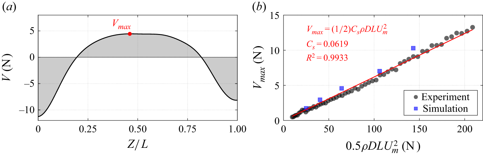
appears near the midpoint of the pipe in the cases of bidirectionally sheared flow, as figure 6(a) shows, which is different from the classical uniformly loaded beam, where the shear force vanishes at the centre. For a uniformly loaded beam, the shear force is zero at the midpoint and reaches its maximum magnitude at the supports on both ends (Clough & Penzien Reference Clough and Penzien2003). This distribution is analogous to the drag force conditions under uniform and linearly sheared flows, where the force exerted along the structure also follows a spatially varying pattern with shear force extrema near the ends. Figure 6(b) illustrates the relationship between the maximum shear force
 $V_{\textit{max}}$
and the dimensionless term
 $0.5 \rho DLU^2$
, across all test conditions. A clear linear correlation is evident, with the fitted data yielding shear force coefficient
 $C_s = 0.0619$
. Similarly, the solid blue squares represent the simulation results, which agree closely with the experimental data and thereby enhance confidence in the simulations, given that both results are processed using the same procedures.
Shear force
 $V$
along the pipe and the maximum shear force in different cases. (a) Shear force
 $V(z)$
distribution (black line) along the pipe at
 $U_m={0.87}\,\mathrm{m\,s^{-1}}\;(Re_m = 2.48\times 10^4)$
based on experimental data. (b) Maximum shear force
 $V_{\textit{max}}$
in different cases (black dots), fitting line (red) with
 $V_{\textit{max}}=(1/2) C_s\rho D L U_m^2$
,
 $C_s = 0.0619$
based on experiment data, and simulation results (solid blue squares).

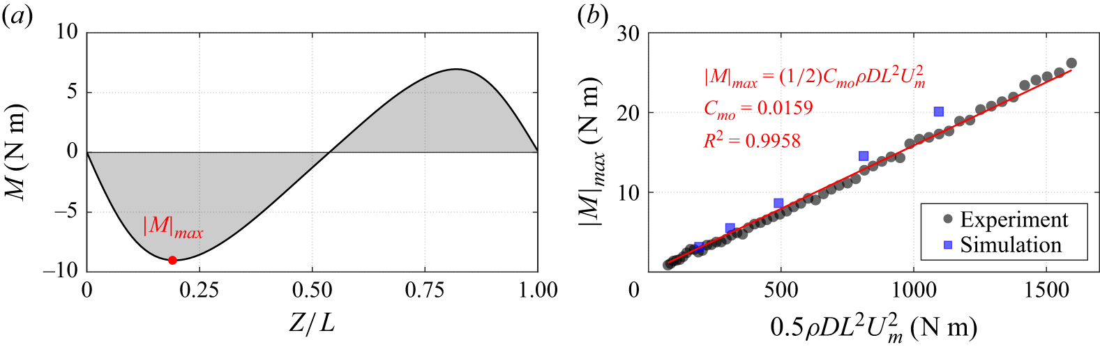
Furthermore, figure 7 illustrates the bending moment distribution based on (3.3). Figure 7(a) displays the distribution for a representative case with
 $U_m = {0.87}\,\mathrm{m\,s^{-1}}\;(Re_m = {24717})$
, revealing a relatively symmetric pattern characterised by two extreme points. The variation
 $\lvert M \rvert _{\textit{max}}$
with flow velocity is also analysed. Using the dimensionless term
 $0.5 \rho D L^2 U^2$
, curve fitting yields bending moment coefficient 0.0159. For VIV of flexible pipes under unidirectional flow (Fu et al. Reference Fu, Fu, Niu, Zhao, Shen and Deng2025b
), the mean displacement in the IL direction does not exhibit the distinct bidirectional distribution observed under bidirectional shear flow, and no extrema of shear force or bending moment appear in the spanwise direction. The solid blue squares represent the simulation results, which agree well with the experimental data.
Based on the above analysis, we draw the following conclusions regarding the first research question posed in § 1.
The bidirectionally sheared inflow introduces a characteristic bidirectional (antisymmetric) mean IL displacement distribution that follows the sign change of the local flow velocity. As shown in figure 3(a),
 $A_{mean}(z)$
exhibits an approximately sinusoidal spanwise variation, and the spanwise maximum
 $A_{\textit{mean},m}$
increases nonlinearly with the mean inflow magnitude, with a dominant quadratic dependence on
 $U_m$
, as shown in figure 3(b). In contrast, the corresponding mean drag coefficient distribution remains largely symmetric with respect to the mid-span: the measured
 $C_d(z)$
is well reproduced by the mirrored profiles over most of the span as shown in figure 4, and the spanwise-averaged value
 $C_{dm}$
stays nearly constant across the tested
 $ \textit{Re}$
range as shown in figure 5(b).
Because the two spanwise halves experience opposite flow directions but similar drag coefficients, the structure is effectively subjected to two opposing mean drag loadings, leading to a non-classical mean shear force distribution with a maximum near the mid-span and a bending-moment distribution with two extrema as shown in figures 6 and 7. These extrema identify the locations where the mean load effects are most pronounced, and therefore provide a physically motivated indication of potential damage-prone regions under bidirectionally sheared flow, which is fundamentally different from the unidirectional flow case where such spanwise extrema of mean shear force and moment do not arise.
Moment
 $M$
along the pipe and the maximum absolute value in different cases. (a) Moment
 $M$
distribution (black line) along the pipe at
 $U_m={0.87}\,\mathrm{m\,s^{-1}}\;(Re_m = 2.48\times 10^4)$
based on experimental data. (b) Maximum absolute value of moment
 $\lvert M \rvert _{\textit{max}}$
in different cases (black dots), fitting line (red) with
 $\lvert M \rvert _{\textit{max}}=( 1/2) C_{mo}\rho D L^2 U_m^2$
,
 $C_{mo} = 0.0159$
based on experimental data, and simulation results (solid blue squares).

3.3. Flow velocity distribution effect
As stated in § 2, the bidirectionally sheared flow generated by the circular rotating apparatus is not perfectly symmetric in the experiments, exhibiting an offset of approximately
 $4.5\,\%$
with only small variations due to pipe vibration; accordingly, we represent the velocity profile as
 $[-0.95Re_m,Re_m]$
. By contrast, the numerical simulations assume a perfectly antisymmetric flow velocity distribution over the spanwise direction. Here, we consider the experimental offset to cross-validate the credibility of the experimental and numerical simulation results, which also provides supporting evidence that our experimental set-up can effectively generate the bidirectionally sheared flows. Moreover, numerical simulations are employed to investigate the mean displacement characteristics under two non-symmetric flow velocity distributions to investigate the flow velocity distribution effect.
Shear force
 $V$
and bending moment
 $M$
with different flow velocity
 $ \textit{Re}_r$
distributions. (a) Flow relative Reynolds number
 $ \textit{Re}_r$
distribution. The maximum Reynolds number is fixed as
 $ \textit{Re}_m=2.19 \times 10^4$
with three flow velocity cases by simulation,
 $ \textit{Re}_r\in [-Re_m, Re_m]$
(black line),
 $ \textit{Re}_r\in [-0.75Re_m, Re_m]$
(red dash-dotted line) and
 $ \textit{Re}_r\in [-0.5Re_m, Re_m]$
(blue dashed line), and one case by experiment,
 $ \textit{Re}_r\in [-0.95Re_m, Re_m]$
(green dotted line). (b) Mean displacement
 $A_{mean}/D$
of four cases. (c) Shear force
 $V$
distribution of four cases. (d) Bending moment
 $M$
distribution of four cases.

Figure 8 presents the distributions of the shear force
 $V$
and bending moment
 $M$
under different flow conditions from numerical simulations, characterised by the ranges of relative Reynolds number
 $ Re_r \in[-Re_m, Re_m]$
(black line),
 $ \textit{Re}_r\in [-0.75Re_m, Re_m]$
(red line) and
 $ \textit{Re}_r\in [-0.5Re_m, Re_m]$
(blue line), where
 $ Re_m = 2.19 \times 10^4$
. Figure 8 also show one case obtained from the experiment with
 $ \textit{Re}_r\in[-0.95Re_m, Re_m]$
(green dotted line). As shown in figure 3, the experimental distribution of
 $A_{mean}/D$
is not perfectly antisymmetric because the imposed velocity profile contains a small offset as described in § 2, whereas the numerical results exhibit perfect symmetry by construction. Despite this difference, the experimental and numerical results agree well in overall magnitude, including the extreme values of all three response parameters
 $A_{mean}$
,
 $V$
and
 $M$
as shown in figures 8(b–d). It should also be noted that due to limitations of the current experimental set-up, real-time measurement of the velocity profile offset is not yet feasible; therefore, treating the experimental velocity profile as antisymmetric in future studies is a reasonable approximation. Here, figure 8(a) shows the flow velocity distribution, and figure 8(b) shows the corresponding mean displacement distribution. As the magnitude of flow velocity at
 $Z/L=0$
decreases, the antisymmetric pattern of mean displacement gradually diminishes. When the flow velocity on one side is reduced to half (blue lines), the opposite mean displacement shape disappears (figure 8
b), and the resulting displacement distribution resembles that induced by unidirectional linearly sheared flow (Song et al. Reference Song, Fu, Cao, Ma and Wu2016a
).
Figures 8(c) and 8(d) show the shear force and bending moment distributions of these cases. It is observed that as the edge flow velocity at
 $Z/L=0$
decreases, the shear force value at the corresponding end is reduced. However, the central shear force extrema remain comparable to those under bidirectionally sheared flow with
 $ \textit{Re}_r\in [-Re_m,Re_m]$
, even when the magnitude of the edge velocity is reduced to
 $0.5Re_m$
. In contrast, figure 8(d) shows that the bending moment significantly changes. The antisymmetric bending moment distribution, which resembles the mean displacement pattern, transitions to a profile similar to the linearly sheared flow case when the magnitude of the edge velocity is reduced to
 $0.5Re_m$
.
4. The VIV hydrodynamic properties
In this section, we analyse the VIV hydrodynamic properties based on the numerical simulation results, using the distributed response along the pipe length for hydrodynamic identification. Flow field measurements were not conducted in the present experiments due to practical limitations associated with the long test pipe and the rotating towing apparatus. The inverse finite element method (Wu Reference Wu2011; Song et al. Reference Song, Fu, Cao, Ma and Wu2016a ) is applied to reconstruct the spanwise distribution of hydrodynamic forces. This inverse identification method can produce the continuous force distribution and has been validated with CFD strip force results. The force decomposition introduced later is then applied to obtain the corresponding force components. Previous experimental studies have demonstrated that the flexible pipe VIV exhibits pronounced multi-frequency response behaviour (Bourguet et al. Reference Bourguet, Lucor and Triantafyllou2012, Reference Bourguet, Karniadakis and Triantafyllou2013; Ma et al. Reference Ma, Lin, Fan, Wang and Triantafyllou2022), which becomes more evident in bidirectionally sheared flow (Fu et al. Reference Fu, Fu, Ren, Xie, Xu, Zhang, Liu and Meng2022a , Reference Fu, Zhang, Fu, Zhao, Ren and Xuc ). Conventional least squares (Wu Reference Wu2011), energy-based (Wang et al. Reference Wang, Fan and Triantafyllou2021a ) and Fourier series (Fan et al. Reference Fan, Jodin, Consi, Bonfiglio, Ma, Keyes, Karniadakis and Triantafyllou2019a ) methods have been shown to inadequately capture the hydrodynamic characteristics of VIV with multi-frequency responses. The forgetting-factor least squares method is then employed for the effective identification of multi-frequency VIV hydrodynamics (Liu et al. Reference Liu, Fu, Zhang and Ren2018, Reference Liu, Fu, Zhang, Ren and Xu2020; Fu et al. Reference Fu, Fu, Zhang, Ren, Zhao and Xu2024).
For flexible pipes, the dominant frequency VIV remains the primary concern, as it often contributes most significantly to fatigue damage (Baarholm, Larsen & Lie Reference Baarholm, Larsen and Lie2006). This section first analyses the hydrodynamic forces associated with dominant VIV under bidirectionally sheared flows, followed by an investigation of the time-varying VIV hydrodynamic response.
4.1. Dominant frequency VIV hydrodynamic properties
The VIV hydrodynamic force can be decomposed into the excitation force
 $F_e$
, which is in phase with velocity and represents the energy exchange between the structure and the fluid, and the added mass force
 $F_m$
, which is in phase with acceleration and reflects the added mass effect (Sarpkaya Reference Sarpkaya1995):
 \begin{align} F_y(z,t) = {\underbrace {\frac {1}{2\sqrt {2}\,\dot {\xi }_{y,\textit{rms}}(z)} \rho D\, U^{2}(z)\,C_e(z,t)\, \dot {\xi }_{y}(z,t) }_{F_e}} {\underbrace {\vphantom {\frac {1}{2\sqrt {2}\dot {\xi }_{y,\textit{rms}}(z)} \rho D\, U^{2}\,C_e(z,t)\, \dot {\xi }_{y}(z,t)} -\frac {\pi D^{2}}{4} \rho\, C_m(z,t)\, \ddot {\xi }_y(z,t), }_{{F_m}}} \end{align}
where
 $C_e$
is the excitation coefficient, and
 $C_m$
is the added mass coefficient. This force decomposition has been widely used in engineering practice to support VIV prediction. To obtain the dominant frequency component of the hydrodynamic force, we apply the band-pass filter with range
 $0.8$
to
 $1.2$
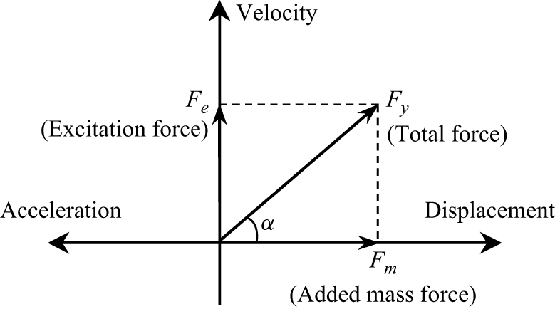
times the sectional vibration dominant frequency obtained from the peak of the power spectral density. Figure 9 schematically illustrates the VIV force decomposition adopted in (4.1). The CF hydrodynamic force
 $F_y$
is expressed as the sum of two components: an excitation force
 $F_e$
, and an added mass force
 $F_m$
. Here, the excitation force
 $F_e$
is in phase with the transverse velocity, and quantifies the portion of the fluid force responsible for energy exchange with the structure. The added mass force
 $F_m$
is in phase with the transverse acceleration, and represents the instantaneous added mass contribution. By projecting
 $F_y$
onto these two orthogonal directions, figure 9 provides a geometric interpretation of how the total VIV force is partitioned between the energy input mechanism
 $F_e$
and the added mass mechanism
 $F_m$
. The angle
 $\alpha$
characterises the relative phase of the resultant force in this reference frame.
Illustration of the VIV force decomposition in (4.1). The total force
 $F_y$
is decomposed into two components:
 $F_e$
, the excitation force that is in phase with the velocity and represents the fluid excitation associated with VIV; and
 $F_m$
, the added mass force that is in phase with the acceleration and represents the instantaneous added mass contribution.

For the dominant hydrodynamic force
 $\kern2pt \hat{\kern-2pt \unicode{x1D641}}_y$
in spatial and temporal distributions, we have
 \begin{align} \hat {\unicode{x1D641}}_y = \overset { \hspace {-1.25em}\substack { \text{spanwise location} \\ \xrightarrow {\quad \quad \quad \quad \quad \quad } } }{ \begin{bmatrix} \hat {F}_y(z_1,t_1) & \hat {F}_y(z_2,t_1) & \cdots & \hat {F}_y(z_n,t_1) \\[5pt] \hat {F}_y(z_1,t_2) & \hat {F}_y(z_2,t_2) & \cdots & \hat {F}_y(z_n,t_2) \\[5pt] \vdots & \vdots & \ddots & \vdots \\[5pt] \hat {F}_y(z_1,t_m) & \hat {F}_y(z_2,t_m) & \cdots & \hat {F}_y(z_n,t_m) \end{bmatrix}_{m \times n} } \begin{array}{@{}l@{}} \\ \Bigg \downarrow {\scriptstyle\text{time}} \end{array} \end{align}
where
 $\hat {({\cdot })}$
represents the dominant frequency part obtained by band-pass filter,
 $\hat {\unicode{x1D641}_{\unicode{x1D66E}}}$
is an
 $ m \times n$
matrix,
 $ n$
represents the number of spanwise locations, and
 $ m$
denotes the number of time steps. Then we have the matrix
 $\unicode{x1D63C}$
as
 \begin{align} {\unicode{x1D63C}} = \overset { {\substack { \text{spanwise location} \\ \xrightarrow {\quad \quad \quad \quad \quad \quad } } }}{ \begin{array}{@{}c@{}} \left [ \begin{array}{ccccc} \mathcal{E}(z_1) \hat {\dot {\xi }}_y(z_1,t_1) & \mathcal{M}(z_1) \hat {\ddot {\xi }}_y(z_1,t_1) & {\cdots} & \mathcal{E}(z_n) \hat {\dot {\xi }}_y(z_n,t_1) & \mathcal{M}(z_n) \hat {\ddot {\xi }}_y(z_n,t_1) \\[5pt] \mathcal{E}(z_1) \hat {\dot {\xi }}_y(z_1,t_2) & \mathcal{M}(z_1) \hat {\ddot {\xi }}_y(z_1,t_2) & {\cdots} & \mathcal{E}(z_n) \hat {\dot {\xi }}_y(z_n,t_2) & \mathcal{M}(z_n) \hat {\ddot {\xi }}_y(z_n,t_2) \\[5pt] \vdots & \vdots & \ddots & \vdots & \vdots \\[5pt] \mathcal{E}(z_1) \hat {\dot {\xi }}_y(z_1,t_m) & \mathcal{M}(z_1) \hat {\ddot {\xi }}_y(z_1,t_m) & {\cdots} & \mathcal{E}(z_n) \hat {\dot {\xi }}_y(z_n,t_m) & \mathcal{M}(z_n) \hat {\ddot {\xi }}_y(z_n,t_m) \end{array} \right ]_{m \times 2n} \\[5pt] {\hspace {-3em}\underbrace {\hspace {8em}}_{\scriptstyle z_1 \;\text{location}}} {\hspace {10em}\underbrace {\hspace {8em}}_{\scriptstyle z_n \;\text{location}}} \end{array} } \begin{array}{l} \Bigg \downarrow {\scriptstyle\text{time}} \end{array} \end{align}
where the size of
 $\unicode{x1D63C}$
is
 $m\times 2n$
, and
 $\mathcal{E}(z)$
and
 $\mathcal{M}(z)$
are the excitation and added mass force non-dimensional items, respectively:
 \begin{align} \mathcal{E}(z) = \frac {\rho D\, U^2(z)}{2\sqrt {2}\, \hat {\dot {\xi }}_{y,\textit{rms}}(z)}, \quad \mathcal{M}(z)=-\frac {\rho \pi D^2}{4}. \end{align}
Considering (4.1) for the dominant hydrodynamic force, the hydrodynamic coefficients at location
 $z_j$
 $(j=1,2,\ldots ,n)$
can be expressed as
 $C_e(z_j)$
and
 $C_m(z_j)$
. Then we have
 \begin{align} \mathcal{\hat {F}}_y(z_j)=\mathcal{A}(z_j)\,\mathcal{C}(z_j), \end{align}
where
 $\mathcal{\hat {F}}_y(z_j)$
is the dominant CF force of location
 $z_j$
in the time domain that is the
 $j$
th column of
 $\hat {\unicode{x1D641}_{\unicode{x1D66E}}}$
in (4.2) with size
 $ m \times 1$
,
 $\mathcal{A}(z_j)$
is the non-dimensional matrix at location
 $z_j$
that is the
 $(2j-1)$
th and
 $(2j)$
th column of
 $\unicode{x1D63C}$
in (4.3) with size
 $ m \times 2$
, and
 $\mathcal{C}(z_j)$
is the hydrodynamic coefficient matrix with size
 $2\times 1$
:
 \begin{align} \mathcal{C}(z_j) = { \begin{bmatrix} C_e(z_j) \\[5pt] C_m(z_j) \end{bmatrix}_{2 \times 1}. } \end{align}
Then we have hydrodynamic coefficients at the
 $z_j$
location based on least squares regression as
 \begin{align} \mathcal{C}(z_j) = \left (\mathcal{A}^{\top} (z_j)\,\mathcal{A}(z_j)\right )^{-1}\mathcal{A}^{\top} (z_j)\,\hat {\mathcal{F}}_y(z_j), \end{align}
and the spanwise distribution of hydrodynamic coefficients can be obtained by traversing the spanwise location. The following linearly sheared flow and uniform flow cases are taken from Fu et al. (Reference Fu, Fu, Niu, Zhao, Shen and Deng2025b ).
Figure 10 presents the simulation results for a unidirectional linearly sheared flow case with
 $U_{m}={0.80}\,\rm{m\,s^{-1}}$
. All panels are generated from the simulation data, and additional details are provided in Fu et al. (Reference Fu, Fu, Niu, Zhao, Shen and Deng2025b
). Figure 10(a) shows the non-dimensional mean displacement
 $A_{mean}/D$
and the RMS CF and IL response amplitudes
 $A_{\textit{CF}}/D$
and
 $A_{IL}/D$
, respectively. Figure 10(b) shows the phase difference between IL and CF directions, expressed as
 \begin{align} \phi _{x y}(z, t)=\left [\phi _{x}(z, t)-\frac {\hat {f}_{x}(z, t)}{\hat {f}_{y}(z, t)} \phi _{y}(z, t) \mod 360^{\circ }\right ] \!, \end{align}
where
 $\phi _{x}(z, t)$
and
 $\phi _{y}(z, t)$
are the instantaneous phases of the dominant IL and CF response, respectively:
 \begin{align} \begin{aligned} \phi _{x}(z, t) &= \mathrm{arg}\big (\hat {\xi }_x(z,t)+\mathrm{i}\,\mathcal{H}(\hat {\xi }_x(z,t)\big ),\\ \phi _{y}(z, t) &= \mathrm{arg}\big (\hat {\xi }_y(z,t)+\mathrm{i}\,\mathcal{H}(\hat {\xi }_y(z,t)\big ). \end{aligned} \end{align}
Here,
 $\mathcal{H}$
represents the Hilbert transform, and
 $\hat {f}_{x}(z, t)$
and
 $\hat {f}_{y}(z, t)$
represent the instantaneous dominant response frequencies at different spanwise locations obtained based on the local maxima of the wavelet transform magnitude. Let
 $\mathcal{W}[\hat {\xi }_x](z, t, f)$
and
 $\mathcal{W}[\hat {\xi }_y](z, t, f)$
denote the wavelet transform of the dominant response in the IL and CF directions. Then the instantaneous dominant frequencies are defined as (Lilly & Olhede Reference Lilly and Olhede2012)
 \begin{align} \hat {f}_x(z, t) = \mathop {\mathrm{arg\,max}}\limits _{f} \big | \mathcal{W}[\hat {\xi }_x](z, t, f) \big |, \quad \hat {f}_y(z, t) = \mathop {\mathrm{arg\,max}}\limits _{f} \big | \mathcal{W}[\hat {\xi }_y](z, t, f) \big |, \end{align}
where
 $\hat {f}_x(z, t)$
and
 $\hat {f}_y(z, t)$
represent the instantaneous dominant frequencies in the IL and CF directions, respectively, obtained by identifying the frequency corresponding to the maximum wavelet transform magnitude at each spanwise location
 $ z$
and time
 $ t$
, and the phase difference of select time is shown as a black line. Figure 10(c) presents the hydrodynamic coefficients determined by (4.7), whereas figures 10(d–h) show the contour of
 $ \omega _z = \partial v / \partial x - \partial u / \partial y$
within the range
 $[-30, 30]$
, corresponding to the red dots highlighted in figure 10(a) with locations
 $Z/L = {1}/{19},{5}/{19},{9}/{19},{13}/{19}, 17/19$
. It should be noted that the results in this section are illustrated based on simulation results.
Dominant hydrodynamic properties along the pipe of the linearly sheared flow case
 $U_{m}={0.80}\,\mathrm{m\,s^{-1}} \; (Re_m = 2.27\times 10^4)$
with unidirectional flow distribution based on numerical simulation data. (a) Spanwise distribution of VIV response of mean displacement (blue dashed line), IL (orange dash-dotted line) and CF (black line) RMS displacement. (b) Histogram of phase difference
 $\phi _{x y}$
, where a selected moment of phase difference is presented as a black line. (c) Excitation (black line) and added mass (red dashed line) coefficient distributions. (d–h) Instantaneous vorticity contours
 $\omega _z$
correspond to the red dots in (a) at locations
 $Z/L = 0.0256, 0.2632, 0.4737, 0.6842, 0.8947$
, with coordinates plotted in metres. Blue to red: negative to positive values with fixed
 $[-30,30]$
range.

In the linearly sheared flow case, the maximum velocity occurs at
 $Z/L = 1$
. As shown in figure 10, the mean displacement exhibits an asymmetric distribution, with larger displacements observed in regions subjected to higher flow velocities. The CF direction is dominated by the first mode response, whereas the IL direction is dominated by the third mode response. A phase jump is observed at the nodes in the IL direction. The hydrodynamic coefficients exhibit stochastic behaviour. The hydrodynamic coefficient
 $C_e$
, associated with the dominant mode of the flexible pipe, is generally correlated with the motion trajectory (Fan et al. Reference Fan, Wang, Triantafyllou and Karniadakis2019b
), whereas
 $C_m$
is typically related to the wake pattern (Wang et al. Reference Wang, Fan and Triantafyllou2021a
). The response characteristics of the flexible pipe become more complex under bidirectionally sheared flow. This study aims to analyse the hydrodynamic properties, with a particular emphasis on evaluating whether the hydrodynamic behaviour of a flexible pipe in a bidirectional flow field resembles that in a unidirectional flow field. Figure 11 presents the simulation results of the dominant VIV result under uniform flow
 $U = {1.4}\,\rm{m\,s^{-1}}$
(
 $ \textit{Re} = 4.34\times 10^4$
). The mean IL displacement exhibits a symmetric distribution around the midpoint, and the phase jump phenomenon is also discovered in the IL VIV displacement node. The spatial distribution of hydrodynamic coefficients likewise reveals more complex variations with higher-order VIV. It can also be observed that the uniform flow case exhibits a more pronounced mean IL displacement shown in figure 11(a). The maximum mean IL displacement exceeds
 $5.0D$
, which shifts the cylinder substantially from its original position in the vorticity contours. In contrast, for the subsequent bidirectionally sheared flow case, the mean IL displacement remains below
 $1.0D$
.
Dominant hydrodynamic properties along the pipe of the uniform flow case
 $U_{m}={1.40}\,\mathrm{m\,s^{-1}}\;(Re_m = 4.34\times 10^4)$
with unidirectional flow distribution based on numerical simulation data. (a) Spanwise distribution of VIV response of mean displacement (blue dashed line), IL (orange dash-dotted line) and CF (black line) RMS displacement. (b) Histogram of phase difference
 $\phi _{x y}$
, where a selected moment of phase difference is presented as a black line. (c) Excitation (black line) and added mass (red dashed line) coefficient distributions. (d–h) Instantaneous vorticity contours
 $\omega _z$
correspond to the red dots in (a), with coordinates plotted in metres. Blue to red: negative to positive values with fixed
 $[-96,96]$
range.

Dominant hydrodynamic properties along the pipe of the bidirectionally sheared flow case
 $U_{m}={0.61}\,\mathrm{m\,s^{-1}}\;(Re_m = 1.73\times 10^4)$
based on numerical simulation data. (a) Spanwise distribution of VIV response of mean displacement (blue dashed line), IL (orange dash-dotted line) and CF (black line) RMS displacement. (b) Histogram of phase difference
 $\phi _{x y}$
, where a selected moment of phase difference is presented as a black line. (c) Excitation (black line) and added mass (red dashed line) coefficient distributions. (d–h) Instantaneous vorticity contours
 $\omega _z$
correspond to the red dots in (a), with coordinates plotted in metres. Blue to red: negative to positive values with fixed
 $[-40,40]$
range.

Figures 12 to 14 present the dominant hydrodynamic properties of the bidirectionally sheared flow cases
 $U_{m}={0.61}$
,
 ${0.99}$
and
 ${1.15}\,\mathrm{m\,s^{-1}}$
, with
 $ \textit{Re}_m$
corresponding to
 $1.73\times 10^4$
,
 $2.81\times 10^4$
and
 $3.27\times 10^4$
, respectively. All panels are generated based on numerical simulation data. The low-velocity region near the midpoint is omitted. Taking the bidirectionally sheared flow condition with
 $U_{m}={0.61}\,\mathrm{m\,s^{-1}}$
as an example, as shown in figure 12, it has been previously demonstrated in figure 3 that the mean displacement of the flexible riser in the IL direction exhibits an antisymmetric pattern under bidirectionally sheared flow. An analysis of the influence of the background current profile on the phase difference of the dominant mode reveals that for VIV under bidirectionally sheared flow, the phase difference generally exhibits an antisymmetric distribution around the midpoint (Wang et al. Reference Wang, Fan, Triantafyllou and Karniadakis2021b
). Phase jumps continue to occur at the nodes of the IL-dominated mode, with phase shift approximately
 $ \pi$
between adjacent regions along the pipe, maintaining an antisymmetric pattern around the midpoint. The dominant mode phase distribution is relevant for semi-empirical prediction studies. The observed phase difference patterns between the dominant CF and IL responses offer valuable insights for guiding future research.
Dominant hydrodynamic properties along the pipe of the bidirectionally sheared flow case
 $U_{m}={0.99}\,\mathrm{m\,s^{-1}}\;(Re_m = 2.81\times 10^4)$
based on numerical simulation data. (a) Spanwise distribution of VIV response of mean displacement (blue dashed line), IL (orange dash-dotted line) and CF (black line) RMS displacement. (b) Histogram of phase difference
 $\phi _{x y}$
, where a selected moment of phase difference is presented as a black line. (c) Excitation (black line) and added mass (red dashed line) coefficient distributions. (d–h) Instantaneous vorticity contours
 $\omega _z$
correspond to the red dots in (a), with coordinates plotted in metres. Blue to red: negative to positive values with fixed
 $[-40,40]$
range.

Dominant hydrodynamic properties along the pipe of the bidirectionally sheared flow case
 $U_{m}={1.15}\,\mathrm{m\,s^{-1}}\;(Re_m = 3.27\times 10^4)$
based on numerical simulation data. (a) Spanwise distribution of VIV response of mean displacement (blue dashed line), IL (orange dash-dotted line) and CF (black line) RMS displacement. (b) Histogram of phase difference
 $\phi _{x y}$
, where a selected moment of phase difference is presented as a black line. (c) Excitation (black line) and added mass (red dashed line) coefficient distributions. (d–h) Instantaneous vorticity contours
 $\omega _z$
correspond to the red dots in (a), with coordinates plotted in metres. Blue to red: negative to positive values with fixed
 $[-70,70]$
range.

Similarly, under bidirectionally sheared flows with
 $U_{m}={0.99}\,\mathrm{m\,s^{-1}}\; (Re_m = 2.81 \times 10^4)$
and
 $U_{m}={1.15}\,\mathrm{m\,s^{-1}}\; (Re_m = 3.27 \times 10^4)$
(as shown in figures 13 and 14), the phase difference exhibits a variation similar to that observed at
 $U_{m}={0.61}\,\mathrm{m\,s^{-1}}$
. As the flow velocity further increases, for the case
 $U_{m}={0.99}\,\mathrm{m\,s^{-1}}$
, a phase jump
 $\pi$
is still observed at the IL nodes; however, a more complex phase transition appears near the mid-span of the model (as shown in figure 13). The cases
 $U_{m}={0.99}\,\mathrm{m\,s^{-1}}$
and
 $U_{m}={1.15}\,\mathrm{m\,s^{-1}}$
exhibit similar phase variation patterns, with the phase difference distribution remaining antisymmetric about the structural midpoint under bidirectionally sheared flow induced VIV.
Further investigations are conducted on the distributions of the excitation force coefficient and the added mass coefficient along the riser. Due to the unique antisymmetric velocity profile of the bidirectionally sheared flow, whether the excitation force coefficient
 $C_e$
exhibits symmetry about the midpoint determines the feasibility of approximating the flow field using a symmetric unidirectional profile (by taking the absolute value of the bidirectional shear flow velocity) for engineering predictions. For the cases discussed in this study, the distribution of the excitation force coefficient generally displays an approximately symmetric pattern about the midpoint, although strict symmetry is not observed. For example, in figure 12(c), the excitation coefficients at both sides exhibit a distribution pattern resembling that of a third-mode-like response, characterised by positive–negative–positive symmetry. A similar distribution is observed in figure 13(c). In figure 14(c), this symmetric variation pattern becomes even more pronounced, with the excitation force coefficient reaching extreme value
 $-1$
. Nevertheless, the patterns near the mid-span boundaries (
 $ Z/L = 0.65$
and
 $ Z/L = 0.35$
) are not completely identical. In the dominant frequency VIV, the added mass coefficients are not always correlated with the wake pattern. For the unidirectional linearly sheared flow case, figure 10(d) displays a P + S wake pattern associated with the negative
 $C_m$
, while figures 10(e–h) exhibit 2S wake patterns with occasional third small vortex and corresponding positive
 $C_m$
values. The high-order uniform flow VIV case does not exhibit a hydrodynamic region with a relatively constant value in figure 11. For bidirectionally sheared flow induced VIV, a pronounced travelling wave phenomenon is observed, and the hydrodynamic force distribution exhibits clear temporal variations. The hydrodynamic characteristics at the dominant frequency are not fully correlated with the wake pattern, shown in supplementary movie 1 for the linearly sheared flow case with
 $U_m={0.80}\,\mathrm{m\,s^{-1}}$
, and in supplementary movie 2 for the bidirectionally sheared flow case with
 $U_m={0.99}\,\mathrm{m\,s^{-1}}$
. However, figures 12 to 14 indicate that at both ends of the pipe, the wake patterns exhibit consistent variation with the added mass coefficient at the dominant frequency; the negative
 $C_m$
corresponds to P + S or 2P wake patterns. The time-varying hydrodynamic properties will be illustrated in the next subsection.
In general, the added mass coefficient
 $C_m$
of a flexible pipe undergoing VIV tends to remain close to
 $1.00$
throughout most of its length, which leads to the choice for the engineering prediction (Wu et al. Reference Wu, Jiang, Lie, Passano, Yin, Sævik, Grytøyr, Hogg, Resvanis and Vandiver2023). In figures 10 and 12 of the low mode VIV presented in the previous subsection, the added mass coefficient in the dominant mode remains close to unity along a large portion of the pipe length.
We apply SPOD in the present study to analyse the dominant frequency connection between the flow field and the flexible pipe (Sieber et al. Reference Sieber, Paschereit and Oberleithner2016; Towne et al. Reference Towne, Schmidt and Colonius2018). The approach used in the present study is the one described by Towne et al. (Reference Towne, Schmidt and Colonius2018). Here, we apply SPOD to the flexible pipe VIV wake based on numerical simulation data to identify the dominant frequency components and associated coherent structures. We define the cross-spectral density matrix at frequency
 $f$
as
 \begin{align} \unicode{x1D64E}(f) = \frac {1}{E} \sum _{n=1}^{E} \hat {\boldsymbol{\omega }}_n(f) \, \hat {\boldsymbol{\omega }}_n(f)^\dagger , \end{align}
where the matrix
 $ \unicode{x1D64E}(f)$
is the cross-spectral density matrix at frequency
 $ f$
, which is constructed by averaging over
 $ E$
overlapping time segments,
 $ \hat {\boldsymbol{\omega }}_n(f)$
denotes the Fourier transform of the
 $ n$
th time window of the spanwise vorticity field
 $ \omega _z(x, y, t)$
at frequency
 $ f$
, and
 $ ({\cdot })^\dagger$
denotes the Hermitian of the argument. The SPOD modes and corresponding energy content are obtained by solving the eigenvalue problem
 \begin{align} \unicode{x1D64E}(f) \, \boldsymbol{\phi }_j(f) = \lambda _j(f) \, \boldsymbol{\phi }_j(f), \end{align}
where
 $\lambda _j(f) \in \mathbb{R}^+$
is the energy of the
 $j$
th mode at frequency
 $ f$
, and
 $\boldsymbol{\phi }_j(f)$
is the spatial structure of the
 $j$
th SPOD mode at frequency
 $f$
. The open implementation of the SPOD algorithm is used in the present study (Schmidt & Colonius Reference Schmidt and Colonius2020), and details can be found in the original source code.
Figures 15 and 16 show the SPOD results for bidirectionally sheared flow cases at
 $U_{m}={0.48}\,\mathrm{m\,s^{-1}}\;(Re_m=1.36\times 10^4)$
and
 $U_{m}={0.99}\,\mathrm{m\,s^{-1}}\;(Re_m=2.81\times 10^4)$
. All panels are generated from the simulation data. For the strips at
 $Z/L=0.10$
and
 $0.30$
, the local flow is from positive to negative, whereas at
 $Z/L=0.70$
and
 $0.90$
, it is from negative to positive. The non-dimensional dominant frequency is defined as
 $f^* = f_{domi}/f_{c1}$
, where
 $f_{domi}$
denotes the peak frequency and
 $f_{c1}$
is the first computed natural frequency listed in table 1, and the
 $f^*$
resolution is approximately
 $0.09$
. In both cases, the first SPOD mode is overwhelmingly dominant, capturing more than
 $99\,\%$
of the total modal energy, and its spatial structure is broadly consistent across strips; the key difference lies in how the dominant frequency varies along the flexible pipe.
The SPOD results at different spanwise locations for the bidirectionally sheared flow case with
 $U_{m} = {0.48}\,\mathrm{m\,s^{-1}}\;(Re_m = 1.36\times 10^4)$
based on numerical simulation data. (a,c,e,g) The SPOD mode 1 energy spectra at
 $Z/L = 0.05$
,
 $0.26$
,
 $0.68$
and
 $0.89$
, respectively. The dominant frequency
 $f^*$
is marked by a red dashed line and labelled at the peak. (b,d,f,h) First spatial SPOD mode at the corresponding dominant frequency, with coordinates plotted in metres. The colour bar range is fixed to
 $[-20, 20]$
for comparison.

For the lower-velocity case
 $U_{m}={0.48}\,\rm{m\,s^{-1}}$
as shown in figure 15, the SPOD peak frequencies in the four strips scale primarily with the local current speed. Specifically, the ratios of the dominant SPOD frequencies are approximately
 $1:0.53:0.37:0.89$
, which are close to the corresponding ratios of the local Strouhal shedding frequencies. We compute local Strouhal shedding frequencies as
 $0.2U(z)/D$
, assuming Strouhal number
 $0.2$
(Bourguet et al. Reference Bourguet, Karniadakis and Triantafyllou2013), which can be estimated as
 $1:0.53:0.41:0.88$
based on the strip Reynolds numbers ratio. This indicates that in this regime, the energetic wake dynamics is governed mainly by the local vortex shedding frequency rather than by the global structural vibration modes.
The SPOD results at different spanwise locations for the bidirectionally sheared flow case with
 $U_{m} = {0.99}\,\mathrm{m\,s^{-1}}\;(Re_m = 2.81\times 10^4)$
based on numerical simulation data. (a,c,e,g) The SPOD mode 1 energy spectra at
 $Z/L = 0.05$
,
 $0.26$
,
 $0.68$
, and
 $0.89$
, respectively. The dominant frequency
 $f^*$
is marked by a red dashed line and labelled at the peak. (b,d,f,h) First spatial SPOD mode at the corresponding dominant frequency, with coordinates plotted in metres. The colour bar range is fixed to
 $[-20, 20]$
for comparison.

For the higher-velocity case
 $U_{m}={0.99}\,\mathrm{m\,s^{-1}}$
as shown in figure 16, our previous experimental study (Fu et al. Reference Fu, Fu, Ren, Xie, Xu, Zhang, Liu and Meng2022
a) showed that the dominant displacement frequency varies along the span, with the mid-span governed by the first mode, and regions near the two ends dominated by the second mode. Here, we have
 $f^*=1$
and
 $f^*=1.99$
corresponding to the first- and second-order structural natural frequencies according to the definition of non-dimensional
 $f^*$
and their values in table 1. Consistent with this trend, the SPOD spectra in figure 16 exhibit dominant peaks that cluster near the first-order (
 $f^*=1$
) and second-order (
 $f^*=1.99$
) structural natural frequencies, even though the corresponding locations are the same as in figure 15 and are not distributed symmetrically. We therefore interpret this higher-velocity regime as a lock-in dominated state, in which the wake dynamics is governed primarily by the structural vibration frequency rather than by the local Strouhal frequency (Bourguet et al. Reference Bourguet, Karniadakis and Triantafyllou2013).
Moreover, the flexible pipe vibrates in both the IL and CF directions and may exhibit different dominant frequencies in each direction, which can jointly influence the SPOD results. However, CF vibration is typically more important because it has larger amplitudes and contributes more to fatigue damage (Huera-Huarte Reference Huera-Huarte2025). Here, the peak frequencies associated with the leading SPOD modes shown in figures 15 and 16 are closely aligned with the dominant response frequency of VIV in the CF direction instead of the IL direction, which indicates that the dominant fluid energy distribution is primarily aligned with the CF vibration pattern. Overall, the SPOD results serve here as supporting evidence for a transition from Strouhal-governed wake dynamics at lower velocity to lock-in governed wake dynamics at higher velocity in bidirectionally sheared flow, and meanwhile SPOD offers an efficient framework for studying the VIV lock-in phenomenon.
Based on the above analysis, we draw the following conclusions regarding the second and third research questions posed in § 1.
-
(i) Effect of the antisymmetric velocity distribution on the VIV phase. The unique antisymmetric velocity distribution of the bidirectionally sheared flow does not alter the phase distribution of the VIV response. A clear phase jump of approximately
 $\pi$
is consistently observed at the IL nodes shown in figures 12(b), 13(b) and 14(b), indicating that the fundamental phase jump phenomenon remains unchanged under bidirectionally sheared flow.
-
(ii) Symmetry of the excitation coefficient at the velocity reversal point. The excitation force coefficient
$C_e$
exhibits a reasonably symmetric distribution about the flow velocity reversal point, suggesting that the two half-spans contribute in a nearly mirrored distribution shown in figures 12(c), 13(c) and 14(c). This symmetry indicates the potential to simplify a bidirectionally sheared flow case into two separate unidirectional sheared flow cases for engineering prediction purposes.


The property of the added mass coefficient distribution requires further time-domain investigation, and will be discussed in the following subsections.
4.2. Time-varying hydrodynamic properties
In the previous subsection, the hydrodynamic forces at the dominant frequency were obtained using the least squares method. However, the least squares approach performs poorly in identifying multi-frequency VIV responses and capturing time-varying coefficients (Liu et al. Reference Liu, Fu, Zhang and Ren2018). The forgetting-factor least squares algorithm (Fortescue, Kershenbaum & Ydstie Reference Fortescue, Kershenbaum and Ydstie1981) is a variant of least squares estimation that was originally developed in the adaptive control community. It has been applied in VIV research to identify time-varying hydrodynamic coefficients (Liu et al. Reference Liu, Fu, Zhang, Ren and Xu2020). Here, we define
 \begin{align} \begin{aligned} {\unicode{x1D641}_y^{\kern1pt *}}(z,t_s)&={\unicode{x1D643}^{\kern1pt *}_{{s}}}(z,t_s)\,\boldsymbol{\theta }_s(z,t_s),\\{\unicode{x1D641}_y^{\kern1pt *}}(z,t_s)&=\left [\beta ^{s-1}\,F_{y}\left (z,t_{1}\right ), \beta ^{s-2}\,F_{y}\left (z,t_{2}\right ), \beta ^{s-3}\,F_{y}\left (z,t_{3}\right ), \ldots ,\beta ^0\, F_{y}\left (z,t_{s}\right )\right ]^{^\top} _{s\times 1},\\{\unicode{x1D643}^{\kern1pt *}_{{s}}}(z,t_s)&=\left [\begin{array}{cccc} \beta ^{s-1}\,\mathcal{E}^*(z,t_1)\,\dot {\xi }\left (z,t_{1}\right ) &\beta ^{s-2}\,\mathcal{E}^*(z,t_1)\,\dot {\xi }\left (z,t_{2}\right ) &\ldots &\mathcal{E}^*(z,t_1)\,\dot {\xi }\left (z,t_{s}\right ) \\[5pt]\beta ^{s-1}\,\mathcal{M}^*(z)\,\ddot {\xi }\left (z,t_{1}\right ) &\beta ^{s-2}\,\mathcal{M}(z)\,\ddot {\xi }\left (z,t_{2}\right ) &\ldots &\mathcal{M}(z)\,\ddot {\xi }\left (z,t_{s}\right ) \end{array}\right ]^{^\top} _{s\times 2},\\\boldsymbol{\theta }(z,t_s)&=\left [\begin{array}{c} C_e\left (z,t_{s}\right ) \\[5pt]C_m\left (z,t_{s}\right ) \end{array}\right ]_{2\times 1},\\s&\in \mathbb{N}^+, \quad 1 \leqslant s \leqslant m, \end{aligned} \end{align}
where
 $\beta \in (0,1]$
provides different weights on data at different times,
 $\beta =1.00$
corresponds to the ordinary least squares algorithm, and
 $\mathcal{E}^*(z,t_s)$
is the time-varying excitation dimensional item:
 \begin{align} \mathcal{E}^*(z,t_s) = \frac {\rho D\, U^2(z)}{2\, \left |\dot {\xi }_{y}(z,t_s)\right |}. \end{align}
Based on the least squares fit algorithm, the parameters to be identified need to minimise the sum of the squared errors between
 ${\unicode{x1D641}_y^{\kern1pt *}}(z,t_s)$
and
 ${\unicode{x1D643}^{\kern1pt *}_{{s}}}(z,t_s)\,\boldsymbol{\theta }_s(z,t_s)$
as
 $J(\boldsymbol{\theta })$
, which follows
 \begin{align} \left .\dfrac {\partial J(\boldsymbol{\theta })}{\partial \boldsymbol{\theta }}\right |_{\hat {\boldsymbol{\theta }}_s}=\left .\dfrac {\partial }{\partial \boldsymbol{\theta }}\big ({\unicode{x1D641}_y^{\kern1pt *}}(z,t_s)-{\unicode{x1D643}^{\kern1pt *}_{{s}}}(z,t_s)\,\boldsymbol{\theta }_s(z,t_s)\big )^{\top} \big ({\unicode{x1D641}_y^{\kern1pt *}}-{\unicode{x1D643}^{\kern1pt *}_{{s}}}(z,t_s)\,\boldsymbol{\theta }_s(z,t_s)\big )\right |_{\widehat {\boldsymbol{\theta }}_s}={0}. \end{align}
Then we have
 \begin{align} \begin{aligned} \hat {\boldsymbol{\theta }}_s(z,t_s) & =\big ({\unicode{x1D643}^{\kern1pt *}_{{s}}}^{\top} (z,t_s)\, {\unicode{x1D643}^{\kern1pt *}_{{s}}}(z,t_s)\big )^{-1} {\unicode{x1D643}^{\kern1pt *}_{{s}}}^{\top} (z,t_s)\, {\unicode{x1D641}_y^{\kern1pt *}}(z,t_s)\\&=\big ({\unicode{x1D643}_{{s}}}^{\top} (z,t_s)\, \unicode{x1D647}_{s} {\unicode{x1D643}_{{s}}}(z,t_s)\big )^{-1} \unicode{x1D643}_{{s}}^{\top} (z,t_s)\, \unicode{x1D647}_{s} {\unicode{x1D641}_y}(z,t_s), \end{aligned} \end{align}
where
 $\unicode{x1D647}_s$
is the weighted matrix, which is a diagonal matrix
 $\unicode{x1D647}_s=\mathrm{diag} (\mu ^{s-1},\mu ^{s-2},\ldots ,\mu ,1)$
,
 $\mu = \beta ^2,\ \mu \in (0,1]$
, and
 $\mu$
is called the forgetting factor. The essence of this method is to assign lower weights to the data farther from the current moment of estimation. By traversing the spanwise positions
 $z$
and the time sequence, the time-domain distributions of the excitation coefficients and added mass coefficients along the riser can be obtained. The time-domain hydrodynamic coefficients exhibit complex temporal variations, as shown in the supplementary movies 1 and 2.
Instantaneous VIV hydrodynamics for linearly sheared flow case
 $U_{m}={0.80}\,\rm{m\,s^{-1}}$
of simulation at
 $Z/L=0.80$
location based on numerical simulation data. (a) The VIV response in the CF direction (black line) and the IL direction (blue line) in the time domain. (b) Excitation (black line) and added mass (black dashed line) coefficients in the time domain. (c–f) Instantaneous vorticity contours
 $\omega _z$
at different time stamps corresponding to the red dots in (a) and (b) from left to right (red dashed line), with
 $[-35,35]$
range. (c,d,e) The 2S wake pattern; (f) the P + S wake pattern. Negative
 $C_m$
in (c) and (f).

Instantaneous VIV hydrodynamics for bidirectionally sheared flow case
 $U_{m}={0.99}\,\mathrm{m\,s^{-1}}$
of simulation at
 $Z/L=0.90$
location based on numerical simulation data. (a) The VIV response in the CF direction (black line) and the IL direction (blue line) in the time domain. (b) Excitation (black line) and added mass (black dashed line) coefficients in the time domain; the grey line represents the zero value. (c–f) Instantaneous vorticity contours
 $\omega _z$
at different time stamps corresponding to the red dots in (a) and (b) from left to right (red dashed line), with
 $[-35,35]$
range. (c,d) The 2S wake pattern; (e) the P + S wake pattern; (f) the 2P wake pattern. Positive
 $C_m$
in (c); negative
 $C_m$
in (d–f).

The time-domain characteristics of the added mass coefficient are more complex due to multi-mode and travelling wave phenomena (Huera-Huarte Reference Huera-Huarte2025). In previous studies of VIV under uniform flow, negative added mass coefficients are generally associated with P + S or 2P wake patterns (Wang et al. Reference Wang, Fan and Triantafyllou2021a ). However, the travelling wave behaviour of the flexible riser leads to more complex and unsteady wake shedding patterns. The analysis is further extended to investigate this phenomenon by conducting an examination of the time-domain hydrodynamic forces at different sections of the flexible riser under various flow conditions.
Figure 17 shows the instantaneous VIV hydrodynamic coefficients for the linearly sheared flow case
 $U_{m}={0.80}\,\rm{m\,s^{-1}}$
based on simulation results at the
 $Z/L=0.80$
location. Figure 17(a) shows the IL and CF VIV responses in the time domain, figure 17(b) shows the instantaneous excitation coefficient
 $C_e(t)$
and added mass coefficient
 $C_m(t)$
based on (4.16), and figures 17(c–f) show the instantaneous vorticity contours
 $\omega _z$
related to the red dot (left to right) time stamp. Figure 18 presents the time-domain vortex-induced hydrodynamic forces at cross-sections of the riser under the bidirectionally sheared flow case
 $ U_{m} = {0.99}\,\mathrm{m\,s^{-1}}$
based on numerical simulation results.
In both cases, a pronounced travelling wave response is present. As a result, the VIV response in the time domain is non-stationary and exhibits significant time-varying hydrodynamic characteristics. Examining the wake shedding patterns under the two flow conditions reveals that for the linearly sheared flow case, the wake shedding transitions from the 2S mode to the P + S mode, as shown in figures 17(c–f), accompanied by a change in the added mass coefficient from positive to negative. It should be noted that wake pattern transitions require time to develop. In figure 17(d), the flow experiences only a very short duration with negative
 $C_m$
, during which the wake pattern still exhibits a 2S wake pattern. The transition between different wake patterns remains a subject for future investigation.
For the bidirectionally sheared flow case, the added mass coefficient exhibits a clear time-domain transition from positive to negative. Correspondingly, the wake shedding evolves across four instantaneous vorticity contours through a sequence of 2S (figure 18
c)
 $\rightarrow$
P + S (figure 18
e)
 $\rightarrow$
2P patterns (figure 18
f). Therefore, for both linearly sheared and bidirectionally sheared flows, negative instantaneous
 $C_m$
is consistently associated with the emergence of pronounced P + S and 2P wake patterns, in agreement with observations for uniform flow VIV (Fan et al. Reference Fan, Wang, Triantafyllou and Karniadakis2019b
). In this context, our results indicate that for the final question posed in § 1, the added mass coefficient in bidirectionally sheared flow VIV remains closely linked to the P + S and 2P wake regimes, consistent with prior uniform flow VIV studies.
5. Conclusions and future work
This study investigates the hydrodynamic characteristics of a flexible pipe undergoing vortex-induced vibration (VIV) in bidirectionally sheared flow, inspired by subsurface currents induced by internal solitons, which occur widely in the ocean. Through a combination of experimental measurements and validated numerical simulations, the effects of antisymmetric background flow on the structural response and hydrodynamic properties are systematically explored. The Reynolds number in the present study ranges from
 $8523$
to
 $39\,490$
, which lies within the subcritical regime (Achenbach Reference Achenbach1971). This range covers most Reynolds numbers commonly investigated in VIV studies (Trim et al. Reference Trim, Braaten, Lie and Tognarelli2005; Vandiver et al. Reference Vandiver, Marcollo, Swithenbank and Jhingran2005; Fan et al. Reference Fan, Wang, Triantafyllou and Karniadakis2019b
). However, extending the analysis to higher Reynolds numbers is necessary to more systematically characterise VIV response under bidirectionally sheared flow.
The mean in-line (IL) displacement exhibits a nearly antisymmetric distribution, and a quadratic relation is observed between the maximum displacement and flow velocity. The mean drag coefficient remains nearly constant across different Reynolds numbers, with average value
 $\overline {C_{dm}} = 1.47$
, showing that the mean drag coefficient only has a weak dependence on the flow velocity of bidirectionally sheared flows. The resulting shear force and bending moment distributions differ from those in uniform flow VIV, exhibiting a maximum shear force near the mid-span, and an antisymmetric bending moment profile resembling a sinusoidal function along the spanwise direction. Corresponding empirical formulas for the peak shear force and maximum moment are proposed. The relationship between spanwise distributions of VIV response and drag coefficients remains unclear and will be a topic for further investigation.
The dominant frequency hydrodynamic analysis shows that the coefficient
 $C_e$
distribution is approximately symmetric about the mid-span, whereas the added mass coefficient
 $C_m$
remains close to unity over most of the length. The phase difference between the cross-flow and IL responses retains an antisymmetric pattern, with phase jumps of nearly
 $\pi$
at the nodes of IL modal shapes. In the time domain, significant unsteadiness in the hydrodynamic coefficients is captured using the forgetting-factor least squares approach. Notably, negative instantaneous added mass coefficients are observed during transitions to P + S and 2P wake patterns, indicating a strong correlation between unsteady wake dynamics and added mass variation. However, the relationship between added mass oscillations and wake-pattern transitions remains unclear, and further research for higher
 $ \textit{Re}$
is needed to examine transition intermittency and hysteresis, using either scaled experiments with particle image velocimetry (Raffel et al. Reference Raffel, Willert, Scarano, Kähler, Wereley and Kompenhans2018) or complementary CFD studies.
Spectral proper orthogonal decomposition (SPOD) of the flow field provides further insights into flow–structure interaction. At lower flow velocities, the dominant frequency distribution closely follows the background velocity profile, indicating that the fluid dynamics are governed by the Strouhal law. At higher velocities, the dominant frequencies become symmetric and align with the structural vibration dominant frequency distribution, suggesting SPOD as a new analysis tool for the lock-in phenomenon in flexible pipe VIV.
The present study opens several directions for future research. The simulation framework can be extended to more complex pipe systems, such as pipe clusters and configurations with geometric complexity and time-varying flow conditions. In addition, SPOD offers a potential tool for analysing VIV such as connections between the hydrodynamic coefficient and the SPOD result, and mechanism analysis of the flexible pipe lock-in phenomenon (Bourguet et al. Reference Bourguet, Karniadakis and Triantafyllou2013). Fu et al. (Reference Fu, Fu, Niu, Zhao, Shen and Deng2025b ) provided a comprehensive steady flow experimental benchmark dataset for validating the simulation code, and the corresponding hydrodynamic analysis is presented in the current work. However, there are additional VIV experimental phenomena that cannot be fully explained by the experimental results alone, representing a key objective for future simulation efforts. This will also facilitate future work aimed at analysing the shear rate of the flow profile, as systematically investigating the underlying VIV mechanisms across this parameter space through experiment will be conducted in the future.
Supplementary movies
Supplementary movies are available at https://doi.org/10.1017/jfm.2026.11506.
Acknowledgement
X.F., S.F., J.S. and Z.N. gratefully acknowledge the National Science Fund for Distinguished Young Scholars (grant no. 52425102), and continuous support from FIFERS JIP. C.L. receives no support in this work.
Declaration of interests
The authors report no conflict of interest.
Data availability
The data that support the findings of this study are openly available in the GitHub repository https://github.com/xuepengfu/VIVdatashare.
Appendix A. Experimental apparatus credibility analysis
In this appendix, we summarise the credibility analysis of the experimental apparatus based on our published work (Fu et al. Reference Fu, Fu, Ren, Xie, Xu, Zhang, Liu and Meng2022a ), covering five aspects: (1) the influence of the wake generated by the upstream cylinder; (2) the time history of the VIV response; (3) water-depth effects; (4) noise induced by the experimental apparatus; and (5) experimental repeatability.
-
(i) To obtain sufficient strain measurements for VIV analysis, the test pipe completes one full revolution in each run. Because the flow encountered during the second half-revolution is influenced by turbulence generated during the first half-revolution, we evaluate and discuss the effect on the measured VIV strain response. Figure 19 compares the CF strain measurements obtained from one full revolution of the test pipe and from the two half-revolutions separately for a representative case
$U_{m}={0.48}\,\mathrm{m\,s^{-1}}$
. As shown in figure 19(a), the spanwise distributions of the RMS strain
$\varepsilon _{rms}$
from the three datasets nearly collapse over the entire length, with only minor deviations at a few sensor locations, indicating that the overall strain amplitude is insensitive to whether the data are taken from the first half-circle, the second half-circle or the full circle. Consistently, figure 19(b) shows that the strain power spectral densities at
$Z/L=0.50$
exhibit the same dominant frequency peak for all three datasets, while the secondary peaks and broadband levels remain very close. Overall, these comparisons suggest that potential wake effects from the first half-revolution have a negligible influence on the dominant VIV response, and the difference in the overall strain RMS level is
$2.7\,\%$
with limited effect. -
(ii) The VIV time histories were also examined to ensure that a sufficiently long interval of statistically steady response was recorded for subsequent analysis. The results indicate that the time histories of our measurements contain nearly
$50$
VIV response periods, which is at the same level as in the experiment by Trim et al. (Reference Trim, Braaten, Lie and Tognarelli2005), and sufficient for analysis. -
(iii) To minimise free-surface effects, four water depths,
${1.00}$
,
${1.20}$
,
${1.30}$
and
${1.40}\,\mathrm{m}$
, were tested to identify an appropriate experimental depth. The apparatus height is
${0.73}\,\mathrm{m}$
(Fu et al. Reference Fu, Fu, Ren, Xie, Xu, Zhang, Liu and Meng2022a
), and the corresponding distances between the pipe and the free surface are approximately
$9.20D$
,
$16.20D$
,
$19.80D$
and
$23.30D$
, respectively. The overall differences of VIV strain among the four water-depth cases are within
$7\,\%$
. Therefore, the most conservative depth
${1.40}\,\mathrm{m}$
was selected for the formal experiments. -
(iv) As shown in figure 2, the experimental apparatus comprises a complex mechanical system. During operation, these components inevitably generate mechanical noise. We assess the magnitude of this noise by comparing results from air tests and underwater tests. Figure 20 compares the measured strain time histories at
$Z/L=0.50$
for case
$U_{m}={1.39}\,\mathrm{m\,s^{-1}}$
when the pipe is tested in water and when it is operated in air. The strain signal in air remains close to the zero baseline and is at least two orders of magnitude smaller than the VIV-induced strain in water, indicating that the mechanical/electrical background noise is less than
$1\,\%$
of the VIV signal amplitude. Therefore, the influence of the experimental apparatus on the measured VIV strain response is negligible for the present tests. -
(v) One repeat test at
$U_{m}={0.99}\,\rm{m\,s^{-1}}$
was conducted to strengthen the credibility of the VIV measurements. For the repeated run, the relative differences in CF displacement among all measurement points remain below
$5\,\%$
, and the maximum RMS VIV displacement is nearly identical, which demonstrates good experimental repeatability.


Comparison of CF strain data based on the one circle, the first half-circle and the second half-circle in case
 $U_{m} = {0.48}\,\mathrm{m\,s^{-1}}$
(
 $ \textit{Re}_m=1.37\times 10^4$
). (a) The RMS of CF strains at measuring points along the test pipe. (b) Power spectral densities of CF strains at the fifth sensor point of
 $Z/L=0.50$
. Here,
 $\mu \varepsilon$
denotes the microstrain measurement.

Time histories of the measured strain at
 $Z/L=0.50$
for case
 $U_{m}={1.39}\,\mathrm{m\,s^{-1}}$
. The black curve shows the strain recorded in water (VIV response), whereas the red curve shows the strain recorded in air (background mechanical noise). Here,
 $\mu \varepsilon$
denotes the microstrain measurement.

In summary, the above checks indicate that the present experimental facility provides reliable and repeatable measurements for the subsequent VIV hydrodynamic analyses. It should be noted that this appendix only provides a concise credibility summary for completeness, and a more comprehensive assessment of the apparatus and measurement methodology can be found in our previous work, Fu et al. (Reference Fu, Fu, Ren, Xie, Xu, Zhang, Liu and Meng2022a ). In addition to the bidirectionally sheared flow experiments, the updated experimental apparatus has also been used to conduct oscillatory sheared flow VIV experiments, as reported by Fu et al. (Reference Fu, Fu, Zhang, Ren, Zhao and Xu2024).
Appendix B. Modal analysis in VIV experiments
The displacement response in the IL and CF directions is reconstructed using a modal analysis method based on the measured strain data. Figure 21 shows the detailed layout of the CF and IL FBG strain sensors. In total, nine and fourteen sensors are installed to measure strains in the CF and IL directions, respectively. As illustrated in the unfold view, the sensors are distributed along the pipe spanwise coordinate and grouped into four longitudinal arrays as CF1/CF2 and IL1/IL2. The cross-section view shows that the two arrays for each direction are placed at opposite circumferential locations (separated by
 $180^\circ$
), with the CF and IL pairs oriented
 $90^\circ$
apart, enabling independent reconstruction of VIV response in two directions.
Assuming small deformation, the displacement in the CF direction
 $\xi _y(z,t)$
can be expressed as a linear combination of mode shapes:
 \begin{align} \xi _y(z, t)=\sum _{i=1}^{n} q_{i}(t)\, \phi _{i}(z), \quad z \in [0, L], \end{align}
where
 $q_i(t)$
is the time-dependent modal weight, and
 $\phi _i(z)$
is the
 $i$
th spatial mode shape.
The corresponding bending strain
 $\varepsilon _y(z,t)$
is related to the curvature and pipe radius
 $R = D/2$
shown in table 1:
 \begin{align} \varepsilon _y(z,t) = R \frac {\partial ^2 \xi _y}{\partial z^2} = R \sum _{i=1}^n q_i(t)\, \phi _i''(z). \end{align}
For the beam structure with pin–pin end, the
 $i$
th mode shape is
 \begin{align} \phi _i(z) = \sin \left (\frac {i \pi z}{L}\right ), \quad i=1,2,\ldots, \end{align}
with corresponding curvature
 \begin{align} \phi _i''(z) = - \left (\frac {i \pi }{L}\right )^2 \phi _i(z). \end{align}
Thus the strain becomes
 \begin{align} \varepsilon _y(z,t) = - R \sum _{i=1}^{n} \left (\frac {i\pi }{L}\right )^2 q_i(t)\, \phi _i(z). \end{align}
Given the measured strain
 $\varepsilon _y(z,t)$
and known
 $\phi _i(z)$
, the modal weights
 $q_i(t)$
can be identified via projection or regression. The displacement is then reconstructed using (B1). To eliminate high-mode noise, modes are selected based on a curvature RMS threshold: modes with RMS values above 10 % of the maximum are retained (Lie & Kaasen Reference Lie and Kaasen2006).
Distribution of FBG strain sensors along test pipe model. Blue blocks denote the strain sensors in the CF direction, and yellow blocks denote the strain sensors in the IL direction.

This modal reconstruction approach enables time-resolved displacement estimation from distributed strain measurements in both the IL and CF directions. This approach has shown great accuracy for establishing the VIV displacement; more details for this method are provided in Fu et al. (Reference Fu, Fu, Ren, Xie, Xu, Zhang, Liu and Meng2022a ), Huera-Huarte (Reference Huera-Huarte2006) and Lie & Kaasen (Reference Lie and Kaasen2006).