


1. Introduction
The distinguishing trait of viscoelastic fluids is an underlying microstructure that often relaxes on macroscopic time scales. For dilute polymer solutions this microstructure consists of non-interacting macromolecules, the elasticity being endowed by the prolonged relaxation of these molecules on times scales which may range from milliseconds to seconds, and even longer, depending primarily on the polymer molecular weight and solvent viscosity. This elasticity has several striking consequences including rod climbing, die swell and the tubeless siphon effect which are well documented in textbooks (Bird, Armstrong & Hassager Reference Bird, Armstrong and Hassager1987).
The role of elasticity in either suppressing or triggering instabilities in various flows has also been of immense interest due to implications for the polymer and food processing industries. Approximately three decades back, the study of instabilities in polymer solutions received an impetus with the discovery of purely elastic instabilities in flows with curved streamlines, a scenario that includes the canonical viscometric flow geometries (Larson, Shaqfeh & Muller Reference Larson, Shaqfeh and Muller1990; Larson Reference Larson1992; Shaqfeh Reference Shaqfeh1996). Such instabilities are driven by base-state hoop stresses, and the instability sets in above a threshold Deborah number ( ${{De}}$), a dimensionless parameter denoting the ratio of the elastic to the flow time scales, even in the absence of inertia. For large curvature ratios, a statistically stationary disorderly flow results for
 ${{De}}$ values above the threshold, termed elastic turbulence (Groisman & Steinberg Reference Groisman and Steinberg2000).
Elasticity also plays an important role in flows of polymer solutions where inertia is significant; a canonical and important example being the widely studied phenomenon of turbulent drag reduction (Lumley Reference Lumley1969; Virk Reference Virk1975; White & Mungal Reference White and Mungal2008). Simulations of polymers in turbulent channel flow show suppression of the coherent structures characteristic of the buffer layer, such as counter-rotating vortices and streaks aligned with the streamwise direction, in turn leading to a reduced wall shear stress (Sureshkumar, Beris & Handler Reference Sureshkumar, Beris and Handler1997; Dubief et al. Reference Dubief, White, Terrapon, Shaqfeh, Moin and Lele2004; White & Mungal Reference White and Mungal2008). Turbulent drag reduction corresponds mostly to the high  ${{Re}}$ and moderate
 ${{De}}$ regimes. More recently, a novel spatiotemporally chaotic state, dubbed elasto-inertial turbulence, has been shown to arise directly from the laminar state for moderate
 ${{Re}}$ and high
 ${{De}}$, and may be closely linked to the asymptotic regime of maximum drag reduction (Samanta et al. Reference Samanta, Dubief, Holzner, Schafer, Morozov, Wagner and Hof2013; Choueiri, Lopez & Hof Reference Choueiri, Lopez and Hof2018; Garg et al. Reference Garg, Chaudhary, Khalid, Shankar and Subramanian2018; Chandra, Shankar & Das Reference Chandra, Shankar and Das2018; Shekar et al. Reference Shekar, McMullen, Wang, McKeon and Graham2019; Chaudhary et al. Reference Chaudhary, Garg, Subramanian and Shankar2021). These observations call for a deeper mechanistic understanding of the inertial flows of polymeric solutions. The general question of hydrodynamic stability in the
 $({{Re}},{{De}})$ plane is thus an important one, and novel behaviour is expected at large
 ${{Re}}$ and
 ${{De}}$ (Graham Reference Graham2014; Chaudhary et al. Reference Chaudhary, Garg, Shankar and Subramanian2019). Towards this goal, in this paper, we study the linear stability of a vortex column in an elastic liquid (a dilute polymer solution) at large
 ${{De}}$ and
 ${{Re}}$ with the ratio
 ${{De}}/{{Re}}$, known as the elasticity number (
 ${{El}}$), being finite. We demonstrate that the vortex column is susceptible to a novel inertio–elastic instability in this limit.
The early numerical investigations of curvilinear flows in the large  ${{Re}}$,
 ${{De}}$ regime concern the effects of elasticity on flow stability in the Taylor–Couette (Thomas & Walters Reference Thomas and Walters1964, Reference Thomas and Walters1966; Beard, Davies & Walters Reference Beard, Davies and Walters1966) and Dean geometries (Thomas & Walters Reference Thomas and Walters1965) for the inertially dominant case. Apart from analysing the destabilizing effect of elasticity on the centrifugal mode, these early studies led to the identification, for finite
 ${{El}}$, of the so-called inertio–elastic mode in Taylor–Couette flow (Avgousti & Beris Reference Avgousti and Beris1993) that, unlike the centrifugal mode, had an oscillatory character at the onset. More recently, it has been shown that the inertio–elastic mode exists for all Taylor–Couette configurations with a monotonically decreasing angular velocity profile (Ogilvie & Potter Reference Ogilvie and Potter2008). There have been additional investigations of the stability of free shear flows in the inertio–elastic regime. Yarin (Reference Yarin1997) studied the effect of polymer additives on the dynamics of a vortex filament in an ambient shear flow, and showed that vortex stretching associated with the bending mode gets arrested by high longitudinal elastic stresses generated due to stretching of the deformed filament. Azaiez & Homsy (Reference Azaiez and Homsy1994a) analysed the instability of a shear layer, characterized by a hyperbolic tangent velocity profile, in a dilute polymer solution. The fluid rheology was modelled using both quasilinear (Oldroyd-B, corotational Jeffreys) and nonlinear (Giesekus) constitutive relations. The authors were the first to consider the aforementioned distinguished limit,
 ${{De}}, {{Re}} \rightarrow \infty$ with
 ${{El}}$ finite for the Oldroyd-B case, and derived the elastic Rayleigh equation that governs the stability of small-amplitude perturbations to a general parallel shearing flow in this limit. A numerical solution of this equation showed that, for finite
 ${{El}}$, elasticity stabilized the original inertial (Kelvin–Helmholtz) instability of the shear layer by truncating the unstable range of wavenumbers. As argued by Hinch (appendix of Azaiez & Homsy (Reference Azaiez and Homsy1994a)), the stabilizing action of elasticity for long wavelength perturbations is akin to the action of surface tension in damping out transverse modulations of a stretched membrane, the tension being on account of the stretched polymers in the region of high shear (the ‘membrane’). Later, motivated by the stability of vortical structures that result from the roll up of an elastic shear layer, Azaiez & Homsy (Reference Azaiez and Homsy1994b) and Haj-Hariri & Homsy (Reference Haj-Hariri and Homsy1997) studied the role of elasticity on the stability of an unbounded linear flow with elliptical streamlines. Earlier investigations of high-
 ${{Re}}$ flows of Newtonian fluids with elliptical streamlines (Kerswell Reference Kerswell2002) show that the instability of such flows is related to the so-called elliptic instability where a vortex column, subject to an ambient straining flow, is destabilized due to a resonant interaction between pairs of Kelvin modes (Moore & Saffman Reference Moore and Saffman1975). These resonances correspond to points of intersection of the Kelvin dispersion curves, and can only occur in three dimensions (a finite axial wavenumber). In the elastic case, however, Haj-Hariri & Homsy (Reference Haj-Hariri and Homsy1997) found the instability to exist even in two dimensions.
The study most closely related to the current one is that of Rallison & Hinch (Reference Rallison and Hinch1995) who examined the stability of submerged planar and axisymmetric elastic jets. In addition to the expected elasticity-induced modification of the inertial instabilities known for these flow configurations, the authors identified an instability that owes its origin to an interplay of elasticity and inertia. Elastic stresses allow for the propagation of transverse shear waves along the otherwise unperturbed streamlines, and the differential convection by the base-state shear leads to the resonant interaction of a shear-wave pair, in turn leading to exponential growth. The inertio–elastic instability of the vortex column studied here has a similar underlying physical mechanism. An important advantage of the vortex column configuration is that it is inertially stable; as shown recently, the Rankine vortex only supports neutrally stable discrete and continuous spectrum (CS) modes, a combination of which may at best lead to algebraic growth for short times (Roy & Subramanian Reference Roy and Subramanian2014b; Roy Reference Roy2013); analogous results hold for smooth monotonically decaying vorticity profiles. Hence, unlike all earlier efforts (Azaiez & Homsy Reference Azaiez and Homsy1994a; Rallison & Hinch Reference Rallison and Hinch1995; Haj-Hariri & Homsy Reference Haj-Hariri and Homsy1997) where the flow configurations are also susceptible to purely inertial instabilities, the novel inertio–elastic instability in the vortex case exists in isolation. Further, for both the jet and vortex cases, the inertio–elastic instability appears to require a sharp spatial transition from a region that strongly stretches the polymer molecules to a relatively quiescent region where the polymer molecules are close to their equilibrium coil configurations.
In this paper, we examine the aforementioned inertio–elastic instability, analytically for a Rankine vortex, and numerically for other smooth monotonically decreasing vorticity profiles, for two-dimensional disturbances with zero axial wavenumber. The examination of smooth vorticity profiles allows one to verify the requirement of a sharp transition region which, for a vortex column, would be from a central region of solid-body rotation to an irrotational point-vortex exterior. The paper is organized as follows. In § 2, starting from the equations of motion and the Oldroyd-B constitutive relation, we derive the governing linearized equations for small-amplitude perturbations at finite  ${{De}}$ and
 ${{Re}}$. Next, we obtain the elastic Rayleigh equation in plane polar coordinates that governs the stability of a base-state vortical flow to infinitesimal perturbations in the limit
 ${{Re}}, {{De}} \rightarrow \infty$ with
 ${{El}}$ finite. The dimensionless parameter governing stability in this distinguished limit is
 ${E}={{El}}(1-\beta )$. In § 3, we examine the exponential instability that arises for an elastic vortex column via a shear wave resonance; this involves numerically investigating the smooth vorticity profiles above for finite
 ${E}$ (§ 3.1), and an analytical-cum-numerical investigation of the Rankine profile for small
 ${E}$ (§ 3.2). The discrete unstable mode for the Rankine profile is closely related to the elastic CS for small
 $E$. In this limit, it propagates with an angular speed slower than that of the core by an amount of
 $O({E}^{1/2})$ and with a transcendentally small growth rate of
 $O({E}^2 {\rm e}^{-{E}^{-1/2}})$, in units of the core angular velocity, both determined using a matched asymptotics expansion approach; the predictions are in good agreement with numerical results, obtained using a shooting method, for sufficiently high resolution. The transcendental scaling above leads to a precipitous drop in the growth rate for small
 ${E}$ in the numerics, similar to that observed earlier, but not analysed, for the submerged elastic jet (Rallison & Hinch Reference Rallison and Hinch1995). Numerical results for more general vorticity profiles, where the discontinuity in the base-state vorticity of the Rankine vortex is smoothened into a transition layer of width
 $d$, show that the instability persists for non-Rankine profiles, and that the growth rate is of the order of the core angular velocity for finite
 $E$. Finally, in § 4, we summarize the main results with a discussion of future lines of research that emerge from this effort. The vortex stability problem analysed here also has astrophysical ramifications owing to the direct analogy between the governing equations of polymer dynamics for large
 ${{De}}$ and those of magnetohydrodynamics (MHD) at large magnetic Reynolds numbers (
 ${{Re}}_m$); and these are also discussed in § 4.
2. Problem formulation: the elastic Rayleigh equation
The equations of motion and continuity for a polymer solution of density  $\rho$ are given by
 \begin{gather} \rho\frac{{\rm D}\boldsymbol{v}}{{\rm D}t}={-}\boldsymbol{\nabla} p^{*} +\boldsymbol{\nabla} \boldsymbol{\cdot} \boldsymbol{\sigma}_d, \end{gather}
 \begin{gather}\boldsymbol{\nabla} \boldsymbol{\cdot} \boldsymbol{v}=0, \end{gather}
where  ${\boldsymbol \sigma }_d$, the deviatoric stress, is assumed to satisfy the Oldroyd-B constitutive equation and the rescaled pressure,
 $p^{*}$, accounts for the additional (osmotic) pressure induced by polymer molecules. The Oldroyd-B relation is one of the simplest constitutive relations that offers a semiquantitative description of nearly constant viscosity dilute polymer solutions known as Boger fluids (James Reference James2009), and corresponds to a microscopic description where the polymer molecules are modelled as non-interacting Hookean dumbbells (Bird et al. Reference Bird, Armstrong and Hassager1987; Larson Reference Larson1988). For simple shear flow, the Oldroyd-B relation predicts a constant shear viscosity and first normal stress difference coefficient, and a zero second normal stress difference. It is convenient to write
 ${\boldsymbol \sigma }_d$ in (2.1) as the sum of solvent and polymer contributions,
 $\boldsymbol {\sigma }_d=2\mu _s\boldsymbol {E}+G\boldsymbol {A}$. Here,
 ${\boldsymbol E} = \boldsymbol {\nabla } {\boldsymbol v} + (\boldsymbol {\nabla } {\boldsymbol v})^{\dagger}$ is the rate of strain tensor with
 $\mu _s$ being the solvent viscosity. The polymer stress contribution is proportional to the shear modulus
 $G$ with the conformation tensor
 $\boldsymbol {A}\propto \langle \boldsymbol {R R} \rangle$,
 ${\boldsymbol R}$ being the dumbbell end-to-end vector. Since the dumbbells respond affinely to an imposed velocity field in the absence of relaxation,
 ${\boldsymbol A}$ is governed by
 \begin{equation} \overset{\mathcal{5}}{\boldsymbol{A}} ={-}\frac{1}{\tau}(\boldsymbol{A}-\boldsymbol{I}), \end{equation}
where  $\tau$ is the relaxation time and ‘
 $\overset {\mathcal {5}}{}$’ denotes the upper-convected derivative defined by
 \begin{equation} \overset{\mathcal{5}}{\boldsymbol{X}}\equiv\frac{{\rm D}\boldsymbol{X}}{{\rm D}t}-(\boldsymbol{\nabla}\boldsymbol{v})^{{\dagger}} \boldsymbol{\cdot} \boldsymbol{X}-\boldsymbol{X} \boldsymbol{\cdot} (\boldsymbol{\nabla}\boldsymbol{v}), \end{equation}
with  ${{\rm D}}/{{\rm D}t}$ being the material derivative. One may now rewrite the governing set of equations as
 \begin{gather} \rho\frac{{\rm D}\boldsymbol{v}}{{\rm D}t}={-}\boldsymbol{\nabla} p^{*}+\mu_s\nabla^2\boldsymbol{v}+G\boldsymbol{\nabla} \boldsymbol{\cdot} \boldsymbol{A}, \end{gather}
 \begin{gather}\boldsymbol{\nabla} \boldsymbol{\cdot} \boldsymbol{v}=0, \end{gather}
 \begin{gather}\frac{{\rm D}\boldsymbol{A}}{{\rm D}t}-(\boldsymbol{\nabla}\boldsymbol{v})^{{\dagger}} \boldsymbol{\cdot} \boldsymbol{A}-\boldsymbol{A} \boldsymbol{\cdot} (\boldsymbol{\nabla}\boldsymbol{v}) ={-}\frac{1}{\tau}(\boldsymbol{A}-\boldsymbol{I}). \end{gather}
To examine the linearized evolution of two-dimensional disturbances in the swirling flow of an Oldroyd-B fluid, we write  $\boldsymbol {v}=\bar {\boldsymbol {u}}+\boldsymbol {u}, \boldsymbol {A}=\bar {\boldsymbol {A}}+\boldsymbol {a}$ for the velocity and polymer stress fields with the overbar quantities denoting the unperturbed base state. In the regime of interest in this paper (
 ${{Re}}, {{De}} \rightarrow \infty$), any general axisymmetric swirling flow
 $\bar {\boldsymbol {u}}=(0,\varOmega (r) r, 0)$, with
 $\varOmega (r)$ the angular velocity, is an exact solution of the equations of motion. The associated base-state stresses are given by
 $$\begin{gather} \bar{\boldsymbol{A}}=\left[\begin{array}{cc} 1 & r\varOmega'\tau \\ r\varOmega'\tau & 1+2(r\varOmega'\tau)^2 \end{array}\right] \end{gather}$$
in a cylindrical coordinate system where  $'$ denotes a radial derivative. The base-state hoop stress component (
 $\overline {\boldsymbol A}_{\theta \theta }$), on account of the quadratic scaling with the shear rate, becomes dominant for large shear rates (
 $r\varOmega '\tau \gg 1$) except when
 $\varOmega ' = 0$ which corresponds to the trivial case of solid-body rotation. In what follows, we analyse the linear stability of the Rankine vortex profile for which
 $\varOmega (r) = \varOmega _0$ for
 $r< a$ (the rigidly rotating core) and
 $\varOmega (r) = \varOmega _0(a/r)^2$ for
 $r \geq a$ (the irrotational exterior). We also examine the linear stability of more general vorticity profiles numerically.
The governing equation for the perturbation velocity field is
 \begin{equation} \frac{\partial \boldsymbol{u}}{\partial t} + \varOmega\frac{\partial \boldsymbol{u}}{\partial\theta}+\boldsymbol{u} \boldsymbol{\cdot} \boldsymbol{\nabla}\bar{\boldsymbol{u}}={-}\frac{1}{\rho}\boldsymbol{\nabla} p+\nu_s\nabla^2\boldsymbol{u}+\frac{G}{\rho}\boldsymbol{\nabla} \boldsymbol{\cdot} \boldsymbol{a}. \end{equation}
For the two-dimensional perturbations under consideration,  $\boldsymbol {u}\equiv (u_r,u_{\theta })$, and the formulation is more convenient in terms of the axial vorticity,
 $w_z$, which satisfies the following equation:
 $$\begin{align} &\left(\frac{\partial }{\partial t} + \varOmega\frac{\partial }{\partial\theta} \right) w_z + u_r DZ =\nu_s \nabla^2w_z+\frac{G}{\rho}\left\{\boldsymbol{\nabla}\wedge(\boldsymbol{\nabla} \boldsymbol{\cdot} \boldsymbol{a})\right\}_z\nonumber\\ &\quad = \nu_s\nabla^2w_z + \frac{G}{\rho} \left[ \frac{1}{r^2}\frac{\partial^2}{\partial r\partial\theta}(rN_1) + \frac{1}{r}\frac{\partial}{\partial r} \left(\frac{1}{r}\frac{\partial}{\partial r}(r^2a_{r\theta}) \right) - \frac{1}{r^2}\frac{\partial^2}{\partial\theta^2}a_{r\theta} \right] . \end{align}$$
Here,  $D Z=r\varOmega ''+3\varOmega '$ is the base-state vorticity gradient and
 $N_1=a_{\theta \theta }-a_{rr}$ is the perturbation to the first normal stress difference. For the Rankine vortex, the base-state vorticity (
 $Z$) and vorticity gradient (
 $D Z$) are
 $Z(r) = 2\varOmega _0{\mathcal {H}}(a-r)$ and
 $D Z(r) = - 2\varOmega _0 \delta (r-a)$, with
 ${\mathcal {H}}(z)$ and
 $\delta (z)$ being the Heaviside and Dirac delta functions, respectively.
The perturbation elastic stress components that appear in (2.10) obey the following equations:
 \begin{align} &\left(\frac{\partial }{\partial t}+\varOmega\frac{\partial }{\partial\theta}+\frac{1}{\tau}\right)a_{rr}-2\left\{\bar{A}_{rr}\frac{\partial u_r}{\partial r}+\frac{\bar{A}_{r\theta}}{r}\frac{\partial u_r}{\partial\theta}\right\}=0, \end{align}
 \begin{align} &\left(\frac{\partial }{\partial t}+\varOmega\frac{\partial }{\partial\theta}+\frac{1}{\tau}\right)a_{r\theta}+\left\{\bar{A}'_{r\theta}u_r-\bar{A}_{r\theta}\left(\frac{\partial u_r}{\partial r}+\frac{u_r}{r}\right)-\frac{\bar{A}_{\theta\theta}}{r}\frac{\partial u_r}{\partial\theta}\right\}\nonumber\\ &\quad + \left\{\bar{A}_{rr}\left(\frac{u_{\theta}}{r}-\frac{\partial u_{\theta}}{\partial r}\right)-\frac{\bar{A}_{r\theta}}{r}\frac{\partial u_{\theta}}{\partial\theta}\right\}-r\varOmega'a_{rr}=0,\end{align}
 \begin{align} &\left(\frac{\partial }{\partial t}+\varOmega\frac{\partial }{\partial\theta}+\frac{1}{\tau}\right)a_{\theta\theta}-2\left\{\bar{A}_{r\theta}\left(\frac{\partial u_{\theta}}{\partial r}-\frac{u_{\theta}}{r}\right)+\frac{\bar{A}_{\theta\theta}}{r}\frac{\partial u_{\theta}}{\partial\theta}\right\}\nonumber\\ &\quad + \left(\bar{A}'_{\theta\theta}-\frac{2\bar{A}_{\theta\theta}}{r}\right)u_r-2r\varOmega'a_{r\theta}=0. \end{align}
We use the vortex core radius  $a$ as the length scale and the turnover time based on the core angular frequency
 $\varOmega _0^{-1}$ as a time scale. Next, assume a normal mode form,
 $h(r,\theta )=\hat {h}(r) {\rm e}^{{\rm i}(m\theta -\omega t)}$, for the various perturbation fields, where
 $m$ is the azimuthal wavenumber and
 $\omega$ is the complex-valued frequency with
 ${\rm Im}(\omega )>0$ corresponding to an exponentially growing perturbation. Thus, from (2.10) and (2.11)–(2.13), we obtain the following non-dimensional equations governing the
 $r$-dependent perturbation amplitudes:
 \begin{gather} \varSigma r\mathscr{L}(r\hat{u}_r) + mrDZ\hat{u}_r = \frac{{\rm i}}{{Re}}r\mathscr{L}^2 (r\hat{u}_r) - \frac{{\rm i}m}{{Ma}^2_e} \left[{-}mD^*\hat{N}_1 + {\rm i}DD^{*}(r\hat{a}_{r\theta}) + \frac{{\rm i}m^2}{r}\,\hat{a}_{r\theta} \right] , \end{gather}
 \begin{gather}\varSigma_2\hat{a}_{rr}=2{\rm i}\left\{\bar{A}_{rr}D+\frac{{\rm i}m\bar{A}_{r\theta}}{r}\right\}\hat{u}_r, \end{gather}
 \begin{gather}\varSigma_2\hat{a}_{r\theta}={-}\frac{r\bar{A}_{rr}}{m}DD^*\hat{u}_r-\left\{\frac{m}{r}\bar{A}_{\theta\theta}+{\rm i}\bar{A}'_{r\theta}\right\}\hat{u}_r+{\rm i}\hat{a}_{rr}r\varOmega', \end{gather}
 \begin{gather}\varSigma_2\hat{a}_{\theta\theta}={-}\frac{2r\bar{A}_{r\theta}}{m}DD^*\hat{u}_r-{\rm i}\left\{\bar{A}'_{\theta\theta}+2\bar{A}_{\theta\theta}D\right\}\hat{u}_r+2{\rm i}\hat{a}_{r\theta}r\varOmega', \end{gather}
where
 \begin{align} D=\displaystyle\frac{{\rm d}}{{\rm d}r},\quad D^*=\displaystyle\frac{{\rm d}}{{\rm d}r}+\displaystyle\frac{1}{r},\quad \varSigma(r)=\omega-m\varOmega(r) \quad {\rm and}\quad \varSigma_2(r)=\omega-m\varOmega(r)+\displaystyle\frac{{\rm i}}{{{De}}} , \end{align}
and the non-dimensional base-state polymeric stresses are given by (2.8) with  $\tau$ replaced by
 ${{De}}$. Here, we have used the relation
 $\hat {w}_z=({\rm i}/m)\mathscr {L}(r\hat {u}_r)$ between the axial vorticity and radial velocity perturbations for zero axial wavenumber with
 $\mathscr {L}=DD^*-(m^2-1)/r^2$ (Roy & Subramanian Reference Roy and Subramanian2014b). The non-dimensional parameters in (2.14)–(2.17) are the Deborah number,
 ${{De}}=\varOmega _0\tau$ which is the ratio of the relaxation to the flow time scale, the Reynolds number,
 ${{Re}}=\varOmega _0a^2/\nu$ based on the total viscosity
 $\mu = \mu _s + \mu _p = \mu _s + G\tau$ and the elastic Mach number,
 $Ma_e=\varOmega _0a/c_{{elas}}$ where
 $c_{{elas}}=\sqrt {G/\rho }$ is the shear wave speed in a quiescent elastic medium. (Note that
 ${{De}}$ is used here instead of the Weissenberg number which is sometimes used in both the drag reduction and elastic instability literature; the distinction between the two parameters is not relevant in the present context.) Similar to its counterpart in compressible flows,
 $Ma_e$ may be interpreted as the ratio of a characteristic flow velocity scale to the speed of propagation of infinitesimal amplitude shear stress (or vorticity) fluctuations in a quiescent incompressible elastic medium. The elastic Mach number may be written in terms of
 ${{Re}}$ and
 ${{De}}$ as
 $Ma_e^2 = ({1}/({1-\beta })){{De}} {{Re}}$,
 $\beta = \mu _s/\mu$ being the ratio of the solvent to the total viscosity, and for a fixed
 $\beta$, the evolution of the perturbations, as governed by (2.14)–(2.17), depends therefore on
 ${{Re}}$ and
 ${{De}}$. Here
 $\beta = 0$ corresponds to a upper-convected Maxwell (UCM) fluid while
 $\beta = 1$ corresponds to a Newtonian fluid; in the latter case,
 $Ma_e \rightarrow \infty$, and (2.14) with only the first term on the right-hand side is the Orr–Sommerfeld equation in cylindrical coordinates.
The above system of equations may be combined into a single fourth-order differential equation governing  $\hat {u}_r$, the cylindrical analogue of the viscoelastic Orr–Sommerfeld equation that has been examined earlier in the context of plane parallel flows (Renardy & Renardy Reference Renardy and Renardy1986). Apart from discrete modes, for any finite
 ${{De}}$ and
 ${{Re}}$, the system (2.14)–(2.17), similar to the case of parallel shear flows, possesses a pair of continuous spectra. The latter are given by
 $r\,\epsilon \,r_c$ with
 $r_c$ defined by
 \begin{gather} \varSigma_2(r_c) = 0, \end{gather}
 \begin{gather}\varSigma(r_c)+\frac{\mathrm{i}}{\beta {{De}}} = 0, \end{gather}
where  $\varSigma _2(r)$ and
 $\varSigma (r)$ are as defined above (Renardy & Renardy Reference Renardy and Renardy1986; Wilson, Renardy & Renardy Reference Wilson, Renardy and Renardy1999; Kupferman Reference Kupferman2005). For
 ${{Re}} = \infty$, there also arises the well known inviscid CS, given by
 $\varSigma (r_c) = 0$, and spanning the base-state range of angular velocities (Roy & Subramanian Reference Roy and Subramanian2014a,Reference Roy and Subramanianb). However, with
 ${{Re}}$ finite and for a bounded domain, the continuous spectra arise solely due to the additional viscoelastic terms (Chaudhary et al. Reference Chaudhary, Garg, Shankar and Subramanian2019).
The relation (2.19) defines the Gorodtsov–Leonov (GL) CS (Gorodtsov & Leonov Reference Gorodtsov and Leonov1967), named after the authors who originally discovered it for inertialess plane Couette flow of a UCM fluid. Although usually studied in the aforementioned specific context owing to its analytical tractability (Graham Reference Graham1998), the GL spectrum continues to exist for finite  ${{Re}}$, and for both parallel shear flows and the azimuthal shearing flows considered here. Its origin is the assumed local nature of the polymeric stress field in almost all constitutive equations in polymer rheology (Bird et al. Reference Bird, Armstrong and Hassager1987). The evolution of the polymeric stress field in the absence of centre-of-mass diffusion is, in fact, similar to that of the vorticity field in the inviscid limit, and both cases, in principle, allow for arbitrarily large gradients across streamlines (Roy & Subramanian Reference Roy and Subramanian2014b,Reference Roy and Subramaniana). Based on this analogy, one expects CS modes with singularities in the polymeric stress fields. The singular GL-eigenfunctions, in addition to being convected with the flow velocity at
 $r= r_c$, decay at a rate
 ${{De}}^{-1}$ due to relaxation, asymptoting to neutral stability for
 ${{De}} \rightarrow \infty$. Further, similar to the plane parallel case, the GL spectrum in cylindrical coordinates is characterized by the Frobenius exponents
 $0, 1, 3$ and
 $4$, the streamline curvature being negligible on the length scales defining the validity of the local Frobenius analysis. An additional CS arises due to a finite solvent viscosity (Wilson et al. Reference Wilson, Renardy and Renardy1999), being pushed off to infinity in the UCM limit (
 $\beta \rightarrow 0$). Again, similar to the parallel flow case, this viscous singular CS has Frobenius exponents – 0, 1, 2 and
 $3-2/\beta$. The final fractional Frobenius exponent indicates the existence of an algebraic branch point and an associated branch cut (Kupferman Reference Kupferman2005). The CS eigenfunctions in this case require, therefore, a principal-finite-part interpretation (Engevik Reference Engevik1971; Gakhov Reference Gakhov1990; Roy & Subramanian Reference Roy and Subramanian2014b).
We now proceed to the regime of interest,  ${{Re}} \rightarrow \infty$ with
 ${{El}} = {{De}}/{{Re}} = \nu \tau /a^2$ fixed, in which case (2.14)–(2.17), with the neglect of the
 $O({{De}}^{-1})$ terms denoting microstructural relaxation, yields the following equation governing
 $u_r$:
 \begin{align}
&\varSigma^3[\varSigma
(r^2D^2\hat{u}_r+3rD\hat{u}_r-(m^2-1)\hat{u}_r)+mrDZ\hat{u}_r]\nonumber\\
&\quad
=2m^2E\varOmega'[\varSigma^2\{r^2\varOmega'D^2\hat{u}_r+r(r\varOmega''+DZ)
D\hat{u}_r\nonumber\\
&\qquad-(m^2-1)\varOmega'\hat{u}_r\}+mr\varOmega'\varSigma\{2r\varOmega'D\hat{u}_r+3(DZ-2\varOmega')\hat{u}_r\}+2m^2r^2
\varOmega'^3\hat{u}_r],
\end{align}
which is the elastic Rayleigh equation with  ${E} = {{El}}(1-\beta )$; the terms proportional to
 ${E}$ in (2.21) denote the contributions due to elasticity. Thus, the original fourth-order ordinary differential equation resulting from (2.14)–(2.17) reduces to a second-order ordinary differential equation in the limit
 ${{De}} \rightarrow \infty$,
 ${{El}},\beta$ fixed, implying that the neglect of relaxation is a singular limit. From what is known for the eigenfunctions of the Rayleigh and Orr–Sommerfeld equations (see section
 $5$ in Roy & Subramanian (Reference Roy and Subramanian2014a)), one expects a non-trivial relationship between the spectrum of the elastic Rayleigh equation and that associated with the full set of equations for large but finite
 ${{De}}$. The viscosity ratio
 $\beta$ no longer plays a fundamental role as for finite
 ${{De}}$ where a non-zero
 $\beta$ leads to an additional CS; in the above limit, one may interpret a change in
 $\beta$ in terms of a rescaled
 ${E}$.
For typical inertio–elastic flows,  ${{El}}$ is the governing parameter only for small but finite
 ${{De}}$ when relaxation effects are dominant and the fluid rheology is describable in terms of a retarded motion expansion (see, for instance, Dabade, Navaneeth & Subramanian (Reference Dabade, Navaneeth and Subramanian2015)). For large
 ${{De}}$, relaxation is unimportant with the dynamics in the polymeric fluid at finite
 ${{Re}}$ being governed by elastic shear waves damped due to the solvent viscosity alone. In this limit,
 $Ma_e$ becomes the governing parameter (Joseph Reference Joseph2007). It is thus a little surprising that in the limit of large
 ${{De}}$ considered here,
 ${{El}}$ rather than
 $Ma_e$ turns out to be relevant for (2.21), suggesting the continued importance of relaxation (
 ${{El}} \propto \tau$). However,
 ${{El}}$ in (2.21) is more appropriately interpreted in terms of a viscoelastic Mach number where the sonic speed corresponds to shear waves propagating in a prestressed elastic medium. The base-state stress level is
 $\bar {A}_{\theta \theta }\sim O({{De}}^2)$ as given earlier, and the shear wave speed relevant to the perturbation dynamics is given by
 $\sqrt {G\bar {A}_{\theta \theta }/\rho } \sim {{De}}\sqrt {G/\rho }$. The relevant Mach number is
 $O({{De}}).O(\sqrt {G/\rho }/\varOmega _0a) \sim ({{De}}/{{Re}})^{{1}/{2}} \sim {{El}}^{{1}/{2}}$. Thus, the rather paradoxical dependence on
 ${{El}}$, and thence on the relaxation time, occurs via the shear wave speed being dependent on the base-state hoop stress. Note that the assumption of the base-state stresses being dependent on the relaxation time, but the perturbations not being sensitive to it, is analogous to the usual assumption for Newtonian fluids where the base state is assumed to be determined by slow viscous diffusion at large
 $Re$, but the latter is nevertheless assumed to play a negligible role in the dynamics of perturbations.
One may rewrite (2.21), in a compact form, in terms of the radial displacement ( $\xi \equiv {\rm i}\hat {u}_r/\varSigma$) as
 \begin{equation} D[r^3PD\xi]=r(m^2-1)P\xi, \end{equation}
where  $P=\varSigma ^2-2m^2{E}\varOmega '^2$. This form was first identified by (Rallison & Hinch Reference Rallison and Hinch1995) in the context of parallel shearing flows. From (2.22), one may easily construct the following modified version of Howard's semicircle theorem (Howard Reference Howard1962) for swirling flows:
 \begin{equation} \left(\omega_r-\frac{m(\varOmega_{{max}}+\varOmega_{{min}})}{2}\right)^2+\omega_i^2 \leq m^2\left(\frac{\varOmega_{{max}}-\varOmega_{{min}}}{2}\right)^2-2m^2{E}\,{\varOmega'_{{min}}}^2. \end{equation}
The role of elasticity is to shrink the inviscid semicircle of instability, implying a relative stabilization. The analogue of (2.22) has been used by Rallison & Hinch (Reference Rallison and Hinch1995) in their study of elastic instabilities in jets. Stability to exponentially growing perturbations results when the semicircle radius decreases to zero, and this happens at a finite  $E$ provided
 $\varOmega '_{min}$ is non-zero. A novel mechanism of instability, associated with the elastic Rayleigh equation, and that may arise even for non-inflectional profiles, is that resulting from the resonant interaction of elastic shear waves. The shear waves propagate more rapidly (relative to the flow) with increasing
 $E$, and the onset of stability above coincides with the inability of the base-state shear, beyond a threshold
 $E$, to bring a pair of such waves into resonance. Note that the form (2.22) also implies the existence of a pair of continuous spectra corresponding to fore- and aft-propagating singular elastic shear waves. The waves propagate with an angular speed of
 $O(\sqrt {{E}})$ relative to the flow, and are obtained by setting
 $P=\varSigma ^2-2m^2{E}\varOmega '^2 = 0$. These travelling-wave spectra are in addition to the original inviscid CS (Case Reference Case1960; Roy & Subramanian Reference Roy and Subramanian2014b) modified by elasticity. Keeping in mind the significance of the elastic CS in interpreting the discrete unstable mode for small
 $E$ (see figure 6 below), a more detailed discussion of the same is included in the supplementary material available at https://doi.org/10.1017/jfm.2022.122.
3. Shear wave resonance instability of a vortex column
In this section, we show that a vortex in a viscoelastic fluid is susceptible to a two-dimensional instability. Towards this end, we first numerically examine the spectra of Rankine-like smooth vorticity profiles as a function of  ${E}$ (§ 3.1). For small
 ${E}$, the unstable eigenfunction is a regularized version of a travelling wave comprising the elastic CS, the travelling wave singularities cut off due to a finite growth rate (see the discussion of the CS in the supplementary material). For the specific case of a Rankine vortex, the elastic instability is then analysed via a matched asymptotic expansions approach valid for small
 ${E}$ (§ 3.2).
3.1. Numerical calculation of the unstable mode
The Rankine vortex has a compact vorticity profile with a step discontinuity at the core radius. A smooth vorticity profile, convenient for use in the numerical calculations below, is given by
 \begin{equation} Z(r) = \frac{Z_0}{2}\left\{1-\tanh\left[\frac{r-a}{d}\right]\right\}. \end{equation}
Here,  $d$ is the length scale over which there is a smooth transition from the core vortical region to the exterior irrotational one, with
 $d \rightarrow$ 0 denoting the limit of a Rankine vortex.
3.1.1. Details of the numerical method
Stability investigations in the limit for large  ${{Re}}$ and
 ${{De}}$ suffer from numerical issues, largely due to the presence of the continuous spectra in the elastic Rayleigh equation (Miller Reference Miller2005). For the problem under consideration, two additional effects make the investigation of the unstable mode a difficult one for small
 $E$. First, the unstable mode asymptotes to a singular neutral mode (a part of the CS) in the limit
 ${E} \rightarrow 0$. This is unlike the classical inviscid problem where the unstable mode approaches a regular neutral mode, the so-called
 $S$-wave, close to the threshold (Drazin & Howard Reference Drazin and Howard1966; Drazin & Reid Reference Drazin and Reid1981). The second reason is the emergence of a transcendentally small length scale for small
 $E$ (identified as part of the analysis in the next section). The inability of the numerics, for a fixed resolution, to resolve the aforementioned small scale, leads to an inevitable breakdown below
 $E\approx 0.02$ regardless of the approach used.
For the smooth monotonically decreasing vorticity profile in (3.1), two separate formulations of the eigenvalue problem in (2.22) are studied. In the first formulation, the linear eigenvalue problem given by (2.14)–(2.17) (in the limit  ${{Re}},{{De}}\rightarrow \infty$) is solved using Chebyshev collocation. In the second formulation, a solution of the nonlinear eigenvalue problem (2.22) for
 $\xi$ is obtained using a compound matrix method wherein the original nonlinear eigenvalue problem is written as a higher-dimensional linear one, which is then solved using standard Chebyshev collocation (Bridges & Morris Reference Bridges and Morris1984; Roy Reference Roy2013). Both formulations yield consistent results, and here we show results from the second formulation (Roy Reference Roy2013). The spectral method obtains the entire eigenspectrum, including the singular elastic continuous spectra alluded to at the end of § 2. Since the CS modes are not
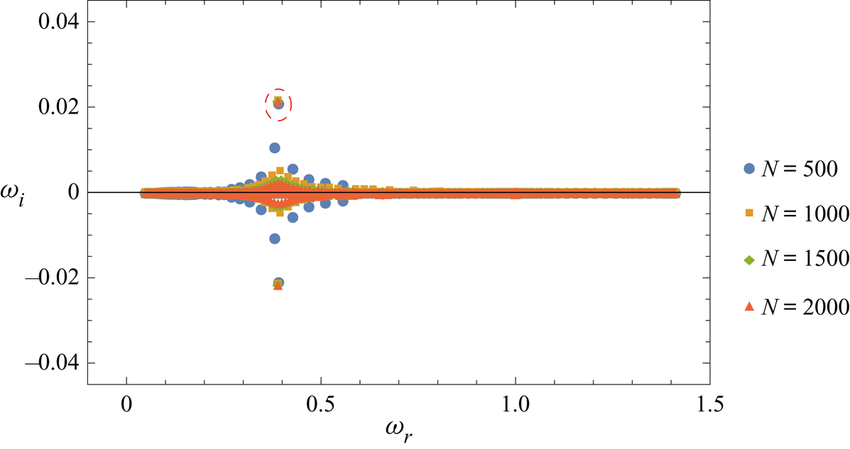
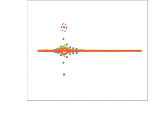
 $C^{\infty }$, the neutral continuous spectra manifest as balloons in the numerical spectrum and for a modest number of collocation points, the ballooned CS ends up engulfing the unstable mode (Roy Reference Roy2013; Chaudhary et al. Reference Chaudhary, Garg, Shankar and Subramanian2019). As shown in figure 1, it is only for a sufficiently large number of collocation points (
 $N$) that the CS balloon shrinks sufficiently for the converged discrete mode to be identified.
Collapse of the ballooned spectrum with increasing number of collocation points ( $N$) for the vorticity profile defined in (3.1) with
 $d=0.025, a=1$ for
 ${E}=0.1$; the domain is
 $r \in (0,r_\infty )$ with
 $r_\infty = 4a$. The converged unstable mode is encircled.

The Rankine vortex, on account of the singular base-state vorticity profile, cannot be studied using spectral methods, and a regular shooting method is applied using the inbuilt bvp4c command in MATLAB. The resolution ( $\tilde {N}$) of the shooting method is controlled by the number of mesh points used for the spatial discretization for the numerical integration in MATLAB. Now
 $\tilde {N}=8000$, unless explicitly mentioned otherwise, for the results obtained below using the shooting method. Here, we only solve (2.22) for
 $r>a$, with appropriate boundary conditions at the core (irrotational) exterior interface (see (3.6)–(3.7) in § 3.2). Owing to the difficulty arising from the extreme sensitivity of the eigenvalue found to the initial guess, we use a ‘carpet bombing’ technique to obtain a reasonably accurate initial guess of the eigenvalue (Miller Reference Miller2005). Herein, one of the boundary conditions is allowed to be an unknown, its difference from the true boundary condition being termed the ‘error’. This error is then minimized on a complex-
 $\omega$ grid to arrive at the initial guess (see Roy (Reference Roy2013) for details).
3.1.2. Numerical results for the inertio–elastic instability
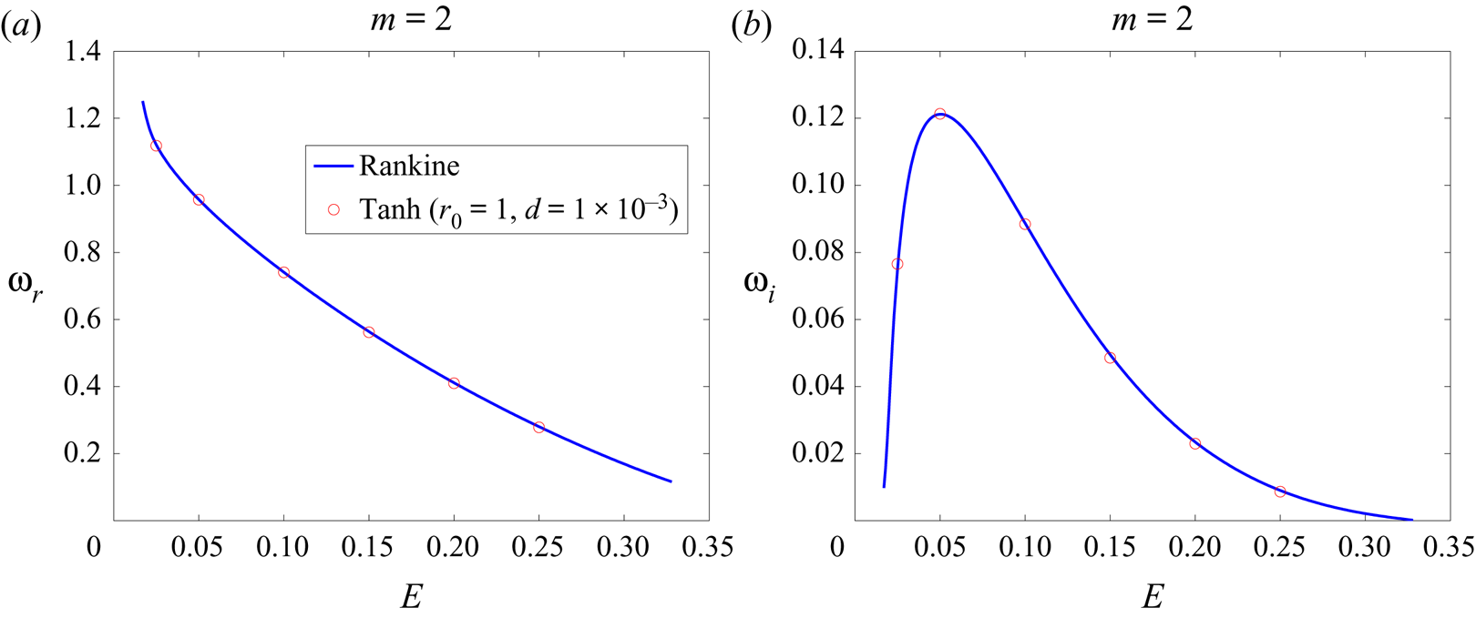
Figure 2(a,b) shows both results from the spectral code (red symbols), for the smooth vortex defined by (3.1) for  $d=10^{-3}$, and that obtained from the shooting method for the Rankine profile. The close comparison of the growth rate and the wave speed shows that an inertio–elastic instability exists for both a Rankine vortex and Rankine-like smooth vorticity profiles. For a smooth profile, one expects the transition width (
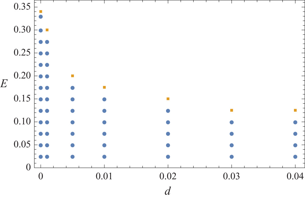
 $d$), the region over which the flow transitions from a rigid-body rotation to an irrotational straining one, to determine the existence of the instability. Expectedly, figure 3 shows that instability exists for a narrower range of
 $E$ with increasing
 $d$.
Wave speed (a) and growth rate (b) comparisons between a Rankine vortex (shooting method) and the smooth vortex in (3.1) with  $a=1$ and
 $d=10^{-3}$ (spectral method), for
 $m=2$. Note that the numerical method does not provide reliable results below
 $E \approx 0.02$, and the suggestion of an elastic threshold in (b) is misleading; the perturbation analysis in § 3.2 shows that the instability persists for any non-zero
 $E$ (also see the higher resolution results, in figure 8, in this regard).

The region of instability for the smooth vortex (3.1) for varying  $E$ and the smoothness parameter
 $d$, with
 $a=1$ and
 $m=2$; the domain is
 $r \in (0,r_\infty )$ with
 $r_\infty = 4a$. The (blue) circles denote the parameters for which a converged unstable mode was obtained, and the (orange) squares denote the parameters for which such a mode could not be found for
 $N$ up to
 $3000$. For
 $d=0$ (the Rankine vortex), the symbols correspond to results obtained using the shooting method.

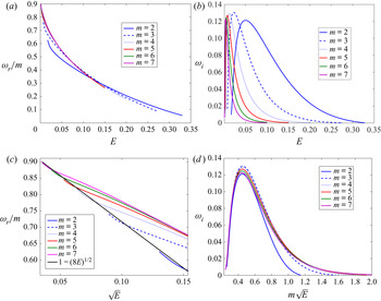
From here on, we focus on the Rankine vortex, and thus all the results presented are computed using the shooting method. Figure 4(a,b) shows the dependence of the wave speed and growth rate of the unstable mode on  ${E}$ for different
 $m$. Figure 4(c) shows the convergence of the wave speeds for different
 $m$ to a common asymptote, given by
 $1- \sqrt {8{E}}$, in the limit
 $E\rightarrow 0$. Figure 4(d) highlights the dependence of the growth rate on the rescaled azimuthal wavenumber
 $m\sqrt {{E}}$. Note that the collapse occurs for
 $m\sqrt {{E}} \sim$
 $O(1)$ and
 $m$ sufficiently large, and accordingly, the curves for the lowest
 $m$
 $(m = 2$ and
 $3$) deviate from the scaled form. Figure 4(d) also shows a rather precipitous drop in growth rate for small
 ${E}$, leading to an eventual breakdown of the numerics (for the chosen resolution) below
 $E\approx 0.02$. As argued in the next section, the steep drop and the associated breakdown arise from a transcendental scaling of the eigenvalue for small
 ${E}$.
Dependence of the wave speed (a) and growth rate (b) on  $E$ for various values of
 $m$. In (c) the phase speed is compared with the leading-order asymptotic solution,
 $\omega _r=m(1-\sqrt {8{E}})$ (§ 3.2), while (d) shows the collapse of the
 $\omega _i$ curves when plotted as a function of
 $m\sqrt {{E}}$. Note that the numerical method does not provide reliable results for
 $\omega _i$ below
 $E \approx 0.02$. However, the perturbation analysis in § 3.2 shows that the instability persists for any non-zero
 $E$.

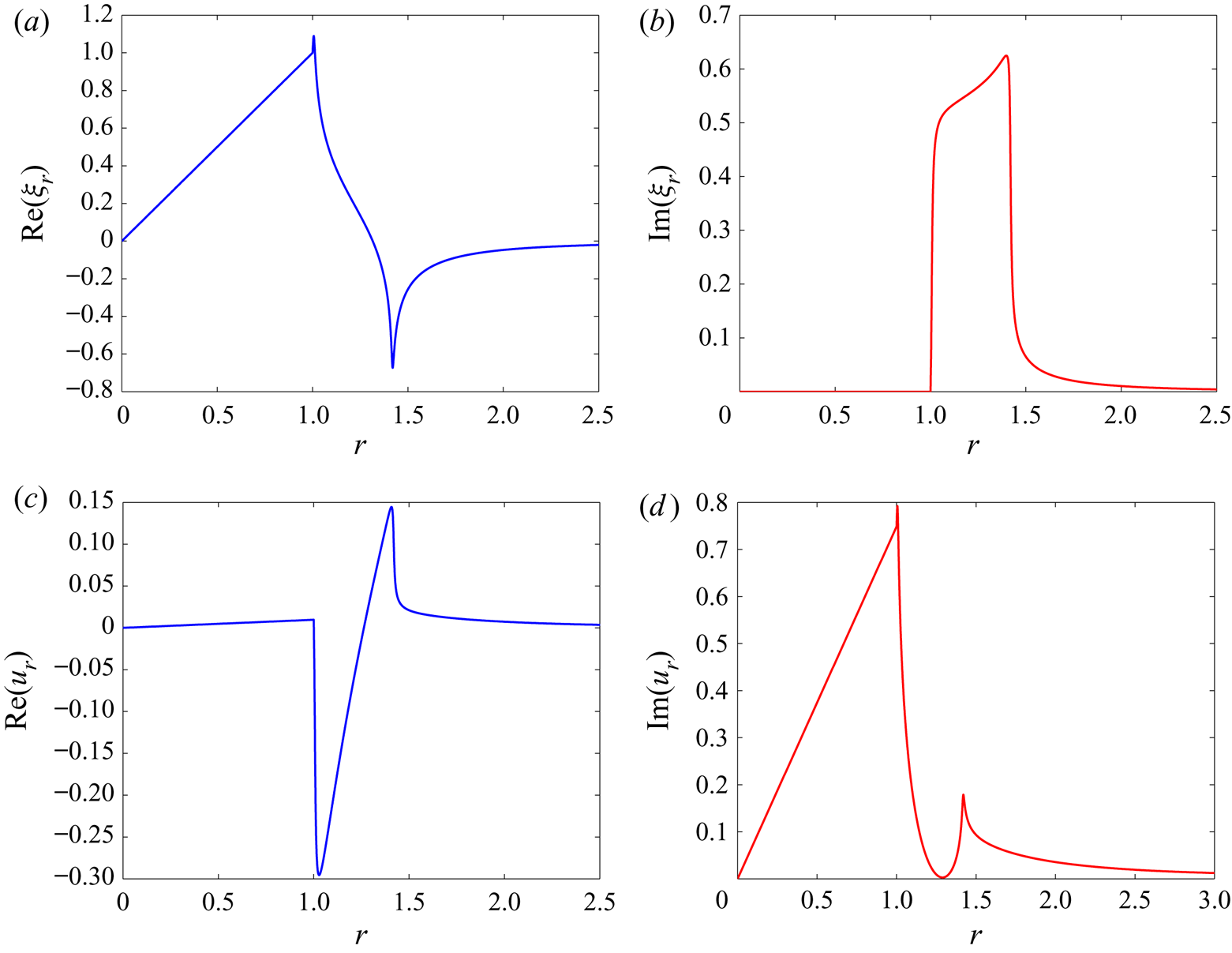
The eigenfunctions for both the radial displacement and velocity fields are shown in figure 5. The twin peaks in the eigenfunction profiles correspond to the fore- (larger  $r$) and aft- (smaller
 $r$) shear wave locations; these peaks become singular in the limit
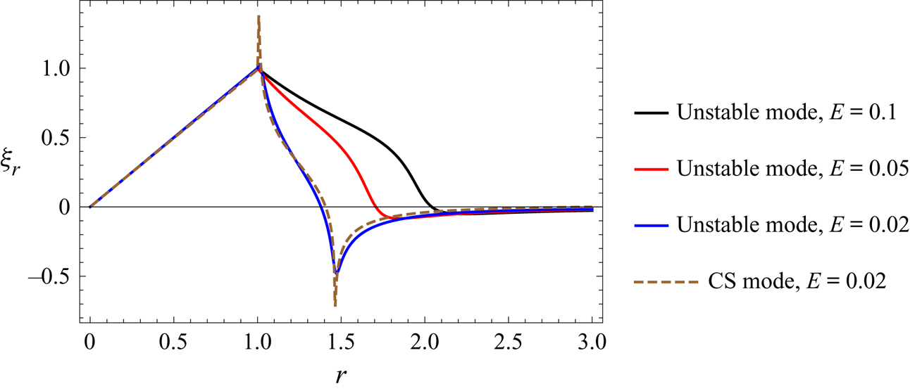
 $E\rightarrow 0$, as the eigenfunction asymptotes to a singular travelling wave eigenfunction in the elastic CS. Figure 6 quantifies this approach by plotting the real parts of the radial displacement eigenfunctions, for a sequence of
 $E$ tending to zero, and a CS eigenfunction for sufficiently small
 $E$. This resemblance, along with the conformance of the wave speed of the unstable mode to the elastic shear wave scaling (
 $\omega _r \sim 1- \sqrt {8{E}}$, see figure 4c), points to the inertio–elastic instability resulting from a resonant interaction between the elastic shear waves, which, for small
 $E$, propagate at nearly the same speed near the vortex core (Rallison & Hinch Reference Rallison and Hinch1995; Miller Reference Miller2005). The shear wave resonance argument also explains why the instability continues to exist for smooth Rankine-like profiles as is seen from figure 3.
Real and imaginary parts of the radial displacement (a,b) and velocity eigenfunctions (c,d) for the unstable mode for  $E=0.017$,
 $m=2$.

Real part of the radial displacement eigenfunction for the unstable mode for varying  $E$; a neutral mode from the CS for
 $E=0.02$, and with the same wave speed, is shown for comparison.

3.2. A matched asymptotic analysis for the inertio–elastic instability of a Rankine vortex:  $E\ll 1$

In this subsection, we analyse the elastic Rayleigh equation, (2.22), for the Rankine profile. This profile exhibits a complete separation of the rotational and straining regions. The polymer molecules in the vortex core are unaffected by solid-body rotation, and retain their equilibrium distribution of conformations. Thus, the polymer stress is homogeneous and isotropic and the solution for  $r < 1$ is identical to the inviscid case, with
 $u_r \propto r^{m-1}$. In order to obtain a normalized radial displacement, the constant of proportionality is chosen to be
 $\varSigma _0 = \omega -m$; as a result,
 $\xi = r^{m-1}$ and
 ${{\rm d}\xi }/{{\rm d}r}|_{r=1-}=m-1$.
The radial displacement in the core, derived above, may now be used as part of a boundary condition for that in the exterior, governed by (2.22) written in an expanded form as
 \begin{equation} D[r^3\{(\omega-m\varOmega)^2-2m^2{E}\varOmega'^2\}D\xi]=r(m^2-1)\{(\omega-m\varOmega)^2-2m^2{E}\varOmega'^2\}\xi. \end{equation}
Noting that the radial displacement is continuous, that is,  $\xi |_{r=1+}\Bigr.=\xi |_{r=1-}\Bigr.=1$ and integrating (2.22) across
 $r=1$, one obtains
 \begin{gather} \quad\left[r^3P\frac{{\rm d}\xi}{dr}\right]_{r=1-}^{r=1+}=0, \end{gather}
 \begin{gather} \Rightarrow \quad \{\varSigma_0^2-8{E}(m\varOmega_0)^2\}\left.\frac{{\rm d}\xi}{{\rm d}r}\right|_{r=1+}-\varSigma_0^2\left.\frac{{\rm d}\xi}{{\rm d}r}\right|_{r=1-}=0, \end{gather}
 \begin{gather} \Rightarrow \quad \left.\frac{{\rm d}\xi}{{\rm d}r}\right|_{r=1+}=\frac{(m-1) (\omega-m)^2}{(\omega-m)^2-8m^2{E}}, \end{gather}
where the expression for the radial displacement gradient in the core is used in the last step. The above condition is combined with the usual requirement of decay in the far field. To summarize the problem statement, the radial displacement in the irrotational exterior satisfies (3.2), and is subject to the following boundary conditions:
 \begin{gather} \xi|_{r=1}=1, \end{gather}
 \begin{gather}\left.\frac{{\rm d}\xi}{{\rm d}r}\right|_{r=1+}=\frac{(m-1) (\omega-m)^2}{(\omega-m)^2-8m^2{E}}, \end{gather}
 \begin{gather}\xi\rightarrow0, \quad \text{as}\ r\rightarrow\infty. \end{gather}
The collapse of the growth rate curves for various  $m$, in figure 4(d), suggests
 $m\sqrt {{E}}$ as the parameter relevant to the asymptotics of the unstable mode for small
 ${E}$. This can also be seen in (3.2), where the term
 $(\omega -m\varOmega )^2-2m^2{E}\varOmega '^2$ involves the interplay of inertia and elasticity, with a balance implying
 $(\omega -m\varOmega )\sim \pm m\sqrt {2{E}}\varOmega '$. For a near-neutral mode, this balance occurs near the vortex core edge,
 $r\approx 1$, implying
 $(\omega -m)\sim \pm m\sqrt {8{E}}$ since
 $\varOmega ' =-2$ at
 $r=1$. Thus, the elastic stresses for this mode are localized about the critical radius,
 $r_c\sim 1+O(\sqrt {{E}})$. This suggests the introduction of a rescaled boundary layer coordinate
 $x = (r-1)/\sqrt {{E}}$ with
 $\omega =m(1-a_1\sqrt {{E}})$, where
 $a_1$ is the unknown eigenvalue. In the limit
 ${E} \rightarrow 0$ with
 $m\sqrt {{E}}$ fixed, this leads to the following simplified equation:
 \begin{equation} \frac{{\rm d}}{{\rm d}\kern0.06em x}\left[\{(a_1-2x)^2-8\}\frac{{\rm d}\kern0.06em \xi}{{\rm d}\kern0.06em x}\right]=m^2 {E} \{(a_1-2x)^2-8\}\xi, \end{equation}
subject to the boundary conditions
 \begin{gather} \xi|_{x=0}=1, \end{gather}
 \begin{gather}\left.\frac{{\rm d}\kern0.06em \xi}{{\rm d}\kern0.06em x}\right|_{x=0}=\sqrt{{E}}\frac{(m-1) (\omega-m)^2}{(\omega-m)^2-8m^2{E}} =m\sqrt{{E}}\frac{a_1^2}{a_1^2-8}, \end{gather}
 \begin{gather}\xi\rightarrow0,\quad \text{as}\ x\rightarrow\infty, \end{gather}
which contain only the parameter  $m \sqrt {{E}}$, as anticipated. The above equation is of the confluent Heun form, although recognition of this fact is not helpful from the perspective of obtaining closed form analytic solutions for
 $m\sqrt {{E}}\sim O(1)$ (Rallison & Hinch Reference Rallison and Hinch1995; Renardy Reference Renardy2008).
Thus, to make analytical progress we consider the alternate limit  ${E}\ll 1$ for
 $m\sim O(1)$. This also helps clarify the absence of a threshold
 ${E}$ for the instability – an aspect that, as already seen, is not resolved by the numerics (as is evident in figure 4d). However, in this limit, apart from the obvious length scale of
 $O(\sqrt {{E}}$), a transcendentally small (in
 ${E}$) length scale emerges from consideration of the boundary conditions. To see this, consider the boundary layer equation (3.9) which takes the form
 \begin{equation} \frac{{\rm d}}{{\rm d}\kern0.06em x}\left[\{(a_1-2x)^2-8\}\frac{{\rm d}\kern0.06em\xi}{{\rm d}\kern0.06em x}\right]=0. \end{equation}
The right-hand side of (3.9) has been discarded, being asymptotically small for  $m\sim O(1)$. Equation (3.13) has solutions of the form
 \begin{equation} \xi=c_1+c_2\log\left[\frac{2x-a_1-\sqrt{8}}{2x-a_1+\sqrt{8}}\right], \end{equation}
with the boundary conditions,
 \begin{gather} \xi|_{x=0}=1 , \end{gather}
 \begin{gather}\left.\frac{{\rm d}\kern0.06em\xi}{{\rm d}\kern0.06em x}\right|_{x=0}=\sqrt{{E}}\frac{(m-1) (\omega-m)^2}{(\omega-m)^2-8m^2{E}}=\sqrt{{E}}\frac{(m-1)a_1^2}{a_1^2-8} , \end{gather}
 \begin{gather}\xi\rightarrow0, \quad \text{as}\ x\rightarrow\infty . \end{gather}
The far-field decay required by (3.17) implies that  $c_1=0$ in (3.14). Applying the gradient boundary condition, (3.16), we have
 $c_2=(m-1)a_1^2\sqrt {{E}}/(8\sqrt {2})$ . Next, considering (3.15), one obtains
 \begin{equation} \xi|_{x=0}=\frac{(m-1)a_1^2\sqrt{{E}}}{8\sqrt{2}}\log\left[\frac{a_1+\sqrt{8}}{a_1-\sqrt{8}}\right]=1. \end{equation}
Since  $a_1\sim O(1)$ the above relation can only be satisfied if
 \begin{equation} a_1=\sqrt{8}+2\sqrt{8}\exp\left({-\frac{1}{m-1}\sqrt{\frac{2}{{E}}}}\right)a_2, \end{equation}
where  $a_2$ is an
 $O(1)$ constant. Although we have added a seemingly exponentially small quantity to the expected
 $O(1)$ estimate, this addition is crucial in the normal displacement boundary condition. With the transcendentally small addition, the normal displacement gradient, given by (3.16), is found to be exponentially large. This obviously contradicts the algebraic scaling assumed in (3.16), and highlights the subtle nature of the small
 ${E}$ limit. Physically, the locations
 $x=a_1+\sqrt {8}$ and
 $x=a_1-\sqrt {8}$ correspond, in rescaled form, to the fore- and aft-moving shear wave singularities. Since
 $a_1-\sqrt {8}\sim \exp ({-({1}/({m-1}))(\sqrt {{2}/{{E}}})})$, the implication is that the aft-travelling shear wave is separated from the edge of the core only by a transcendentally small amount. Note that the above contradiction is not an artefact of the order in which we choose to satisfy the boundary conditions above. The underlying transcendental scaling also explains the precipitous drop in the growth rate (similar to that in figure 4d) of the elastic instability in a submerged jet observed by Rallison & Hinch (Reference Rallison and Hinch1995) – see figure 7 therein.
Thus, we see a crucial difference between the eigenfunction structure in the two limits analysed above. For  ${E} \rightarrow 0$ with
 $m\sqrt {{E}}$ fixed, both the forward- and backward-travelling shear waves lie within a boundary layer with a thickness of
 $\sqrt {{E}}$, next to the vortex core, this being the only length scale of relevance. However, in the limit
 ${E}\ll 1$ for
 $m\sim$
 $O(1)$, the above arguments show that while the forward-travelling shear wave is still localized in an
 $O(\sqrt {{E}})$ boundary layer, the backward-travelling wave is only separated from the edge of the core by a transcendentally small distance of
 $O (\exp ({-({1}/({m-1}))(\sqrt {{2}/{{E}}})}))$. Thus, the perturbation analysis in this latter case needs to recognize two different length scales, one of them exponentially smaller than the other. The asymptotic framework must accordingly include an additional inner boundary layer with
 $r-1\sim O(g\sqrt {{E}})$ satisfying the boundary conditions at
 $r=1$ (
 $g$ will turn out to be transcendentally small). The outer
 $O(\sqrt {{E}})$ boundary layer is therefore no longer constrained to satisfy the boundary conditions at
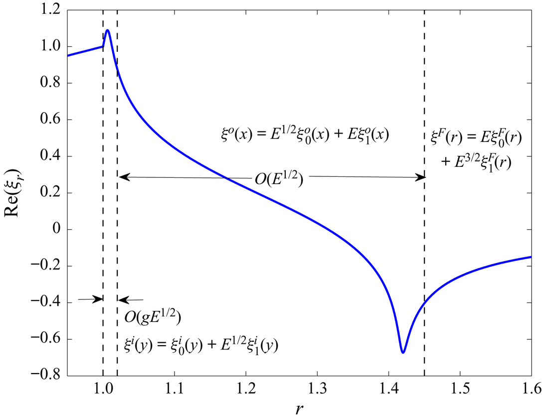
 $r=1$, resolving the contradiction in the naive approach above. Instead, it matches onto both the inner boundary layer and the outer regions in the appropriate limits. Figure 7 shows the different asymptotic regions for a numerically evaluated radial displacement eigenfunction. We thus have the following double expansion, for the eigenvalue, in the limit
 $g \ll 1, {E} \ll 1$:
 \begin{equation} \frac{\omega}{m}=1-\sqrt{{E}}[\sqrt{8}+g \{c_0+c_1\sqrt{{E}}+c_2{E} + c_3{E}^{3/2}+ ...\} +O(g^2)]. \end{equation}
Note that, in neglecting the contributions at  $O(g^2)$ and higher, we anticipate the transcendental smallness of
 $g$ in (3.20), owing to which terms of
 $O(g)$ are, in principle, smaller than any algebraic order in
 $E$; that
 $g\sim \exp ({-({1}/({m-1}))(\sqrt {{2}/{{E}}})})$ emerges from the detailed analysis given below, and the expansion in (3.20) conforms to the exponential asymptotics formalism (Boyd Reference Boyd1999). Note that the
 $O(g)$ contribution is crucial despite its transcendental smallness, since it contributes to the leading-order growth rate. It is shown below that the growth rate is
 $O({E}^2 {\rm e}^{-1/\sqrt {{E}}})$ for small
 $E$, and, therefore, also transcendentally small. Importantly, however, this establishes the absence of a threshold for the elastic instability in contrast to what is suggested by the numerical results above (figure 4d).
Numerically evaluated radial displacement eigenfunction illustrating the nested boundary layer structure that characterizes the small- $E$ asymptotic analysis discussed in the text:
 $r < 1$, the vortex core;
 $r >1$ with
 $r - 1 \sim O(g\sqrt {{E}})$, the inner boundary layer;
 $r >1$ with
 $r-1\sim O(\sqrt {{E}})$, the outer boundary layer;
 $r >1$ with
 $r-1\sim O(1)$, the outer region.

The matched asymptotic expansions approach used here may be validated by consideration of an exactly soluble subproblem – that governed solely by the left-hand side of (3.2) – termed the left-hand side problem herein. The agreement of the asymptotic approach with the small- $E$ expansion of the exact solution serves as a useful validation both of the exponential asymptotics formalism, and the additional subtle feature of phase jumps across the shear-wave singularities; the analysis of the left-hand side problem is detailed in the supplementary material. In what follows, we present a brief synopsis of the analogous analysis, of the full equation (2.22) for small
 $E$, recognizing the different asymptotic regions mentioned above. The detailed analysis is again given in the supplementary material following the analysis of the left-hand side problem.
3.2.1. Outer region: $r-1\sim O(1)$

To begin with, we study the solution in the region where  $r-1\sim O(1)$. Expanding
 $P$ in the elastic Rayleigh equation (2.22) for small
 $E$, one obtains
 \begin{equation} \frac{P}{m^2}=\mathcal{S}_0+\sqrt{{E}} \mathcal{S}_1+{E} \mathcal{S}_2 + {O}(g\sqrt{{E}}), \end{equation}
where
 \begin{equation} \mathcal{S}_0 = \left(1-\frac{1}{r^2}\right)^2,\ \mathcal{S}_1 ={-}2\sqrt{8}\left(1-\frac{1}{r^2}\right) \quad {\rm and}\quad \mathcal{S}_2 = 8\left(1-\frac{1}{r^6}\right). \end{equation}
The expansion of  $P$ has terms which scale algebraically with
 $\sqrt {{E}}$ as well as terms that are transcendentally small (of
 $O(g)$). At leading order, we only need to consider the finite number (three) of terms in (3.21) that scale algebraically. The unknown eigenvalue constants (the
 $c_i$) in (3.20) lead to transcendentally small contributions, and, hence, do not enter the expansion for
 $P$ and the outer region analysis at leading order. Denoting the displacement by
 $\xi ^{F}(r)$, the above points to the following expansion:
 \begin{equation} \xi^F(r)={E} \,\xi^F_0(r)+{E}^{3/2}\,\xi^F_1(r) + {O}({E}^{2})+ {O}(g\sqrt{{E}}), \end{equation}
where we again neglect the transcendentally smaller contributions. While the  $O(E)$ scaling of the leading-order term is evident from the matching considerations below (see § 3.2.4), it may nevertheless be anticipated based on the discussion above. The aft-shear-wave is located in an exponentially small neighbourhood of the edge of the core, and the (logarithmic) displacement due to this wave decreases by
 $O(\sqrt {{E}})$ in the outer boundary layer which is exponentially distant when measured in units of the inner boundary layer thickness of
 $O(g \sqrt {{E}})$. Further, the near cancellation between the
 $O(\sqrt {{E}})$ displacements associated with the fore- and aft-shear-waves for
 $r - 1\sim O(1)$ leads to an asymptotically smaller
 $\xi ^F$ of
 $O(E)$ in this outer region (see figure 7), as assumed in the expansion above. The solution in the outer region, to
 $O({E}^{3/2})$, is as follows:
 \begin{equation} \xi^F(r)={E}\displaystyle\frac{\mathcal{B}_0}{r^{m-1}(r^2-1)}+{E}^{3/2}\left\{\displaystyle\frac{2\sqrt{2}\mathcal{B}_0}{r^{m-1}(r^2-1)^2}+\displaystyle\frac{\mathcal{B}_1}{r^{m-1}(r^2-1)}\right\}+{O}({E}^2). \end{equation}
As already mentioned, the details of the aforementioned solution are given in the supplementary material. In the outer region solution ( $\xi ^F$), there are no signatures of the travelling shear-wave singularities. Note that we do not consider the
 $O({E}^2$) and higher-order contributions to
 $\xi ^F$ since they are not required to determine the growth rate at leading order, an insight that is obtained from the solution of the left-hand side problem.
3.2.2. Outer boundary layer: $r-1\sim O(\sqrt {{E}})$

Having found the solution in the outer region, we now consider the outer boundary layer using the boundary layer coordinate  $x = (r-1)/\sqrt {{E}}$ already introduced at the beginning of this section. Denoting the boundary layer displacement as
 $\xi (r)=\xi ^{o}(x)$, one obtains the rescaled elastic Rayleigh equation as
 \begin{equation} \frac{{\rm d}}{{\rm d}\kern0.06em x}\left[\mathcal{Q}\frac{{\rm d}\kern0.06em\xi^o}{{\rm d}\kern0.06em x}\right]=\frac{{E}\mathcal{Q}(m^2-1)}{(1+\sqrt{{E}}x)^2}\xi^o, \end{equation}
where  $\mathcal {Q}=\displaystyle {(1+\sqrt {{E}}x)^3P}/{m^2{E}}$, and is further expanded as
 \begin{equation} \mathcal{Q}=\mathcal{Q}_0+\sqrt{{E}} \mathcal{Q}_1+{E} \mathcal{Q}_2 +{E}^{3/2} \mathcal{Q}_3+ {O}({E}^{2})+ {O}(g\sqrt{{E}}), \end{equation}
with  $\mathcal {Q}_0=4x(x-2\sqrt {2})$,
 $\mathcal {Q}_1=-12\sqrt {2}x(x-2\sqrt {2})$,
 $\mathcal {Q}_2=x^2(x^2-4\sqrt {2}x-24)$ and
 $\mathcal {Q}_3=x^3(88-x^2)$. Similar to the expansion of
 $P$ discussed earlier in § 3.2.1, the transcendentally small terms are again neglected in (3.26). The displacement
 $(\xi ^o)$ may thus be expanded as
 \begin{equation} \xi^o(x)=\sqrt{{E}} \,\xi^o_0(x)+{E}\,\xi^o_1(x)+{E}^{3/2}\,\xi^o_2(x) +{E}^{2}\,\xi^o_3(x) + {O}({E}^{5/2})+ {O}(g\sqrt{{E}}) . \end{equation}
where the leading  $O(\sqrt {{E}})$ scaling is consistent with the aforementioned physical arguments. Substituting the above expansion into (3.25), one obtains the following equation at
 $O(\sqrt {{E}})$ for the leading-order boundary layer displacement:
 \begin{gather} \frac{{\rm d}}{{\rm d}\kern0.06em x}\left[\mathcal{Q}_0\frac{{\rm d}\kern0.06em\xi_0^o}{{\rm d}\kern0.06em x}\right]=0 \end{gather}
 \begin{gather} \Rightarrow\quad \xi_0^o(x)=\mathcal{G}_{10}+\mathcal{G}_{11}\log\left(\displaystyle\frac{x-2\sqrt{2}}{x}\right). \end{gather}
In the expression above, the forward and backward travelling wave singularities correspond to  $x = 2 \sqrt {2}$ and
 $x = 0$, respectively; the latter location is the edge of the core, since transcendentally small terms are now neglected. The details of the solutions at higher orders are given in the supplementary material.
The constant  $\mathcal {G}_{10}$ in (3.29) is determined via matching, the details of which are again given in the supplementary material. We only note here that in deriving the limiting forms of the above solutions for
 $x \rightarrow 0$, required for matching, one has to account for the multivaluedness of the logarithm in the displacement field (
 $\xi _0^o(x)$) in (3.29). Recall that
 $x = 2 \sqrt {2}$ marks the location (singularity) of the neutrally stable forward-travelling shear wave. The neutral stability arises because the (imaginary) growth rate appears at a higher (and transcendentally small) order in the perturbation expansion. This leads to an ambiguity in the phase jump associated with the logarithm, that is well known in inviscid hydrodynamic stability (Drazin & Reid Reference Drazin and Reid1981). The resolution involves displacing the aforementioned shear-wave singularity off the real axis to
 $x = 2 \sqrt {2} - {\rm i} \epsilon$, with
 $\epsilon > 0$ representative of the small but finite growth rate. As a result, one has
 \begin{align} \log(x-2\sqrt{2} + {\rm i} \epsilon)&=\log|x-2\sqrt{2}|\quad x > 2\sqrt{2},\nonumber\\ &=\log|x-2\sqrt{2}|+{\rm i} {\rm \pi}\quad x<2\sqrt{2}. \end{align}
The above relation may now be used in obtaining the limiting forms of the outer boundary layer solutions.
3.2.3. Inner boundary layer: $r-1 \sim O(g\sqrt {{E}})$

Finally, we introduce an inner boundary layer in an exponentially small neighbourhood of the core, corresponding to  $O(1)$ values of the boundary layer coordinate
 $y = (r-1)/g \sqrt {{E}}$ with
 $g, {E} \ll 1$. Denoting the inner boundary layer displacement as
 $\xi (r)=\xi ^{i}(y)$, we have from (3.2)–(3.7) that
 \begin{equation} \frac{{\rm d}}{{\rm d} y}\left[\mathcal{R}\frac{{\rm d}\kern0.06em\xi^i}{{\rm d} y}\right]=\frac{g^2{E}\mathcal{R}(m^2-1)}{(1+g\sqrt{{E}} y)^2}\xi^i, \end{equation}
with  $\mathcal {R}=(1+g\sqrt {{E}} y)^3P/(m^2g{E})$, which is further expanded as
 \begin{equation} \mathcal{R}=\mathcal{R}_0+\sqrt{{E}} \mathcal{R}_1+ {O}({E}) , \end{equation}
where  $\mathcal {R}_0=4\sqrt {2}(c_0-2y)$ and
 $\mathcal {R}_1=4\sqrt {2}(c_1+6\sqrt {2}y)$. Note that this is the first instance where the unknown eigenvalue constants (the
 $c_i$) enter the expansion. In anticipation of the transcendental smallness of
 $g$, we assume
 $g{E}^{-\alpha }\rightarrow 0$ as
 ${E}\rightarrow 0$,
 $\forall \, \alpha >0$, which allows the neglect of the right-hand side term in (3.2) at all orders. The boundary conditions at the core-exterior interface, (3.6) and (3.7), take the form
 \begin{gather} \xi^i(y=0)=1, \end{gather}
 \begin{gather}\frac{{\rm d}\kern0.06em\xi^i}{{\rm d} y}\left(y=0\right)=(m-1)\sqrt{{E}}\left\{\frac{\sqrt{2}}{c_0}-\frac{\sqrt{2}c_1\sqrt{{E}}}{c_0^2} +... \right\} . \end{gather}
Guided by the above expansions the boundary layer variable,  $\xi ^i(y)$, is expanded as follows:
 \begin{equation} \xi^i(y)=\xi_0^i(y)+\sqrt{{E}}\, \xi_{1}^i(y)+{E}\, \xi_2^i(y)+ {O}({E}^{3/2})+ {O} (g\sqrt{{E}}), \end{equation}
where we note that the radial displacement is now  $O(1)$, as dictated by the boundary condition (3.33). Plugging the above expansion in (3.31) and using the boundary conditions (3.33) and (3.34), we have the following equations (and boundary conditions) and solutions at successive orders.
At  $O{(1)}$ we obtain
 \begin{equation} \frac{{\rm d}}{{\rm d} y}\left[\mathcal{R}_0\displaystyle\frac{{\rm d}\kern0.06em\xi_0^i}{{\rm d} y}\right]=0, \end{equation}
with  $\xi _0^i(y=0)=1$ and
 $({{\rm d}\kern0.06em\xi _0^i}/{{\rm d} y})(y=0)=0$, which gives
 \begin{equation} \xi_0^i(y)=1 . \end{equation}
At  $O{({E}^{1/2})}$ we obtain
 \begin{equation} \displaystyle\frac{{\rm d}}{{\rm d} y}\left[\mathcal{R}_0\displaystyle\frac{{\rm d}\kern0.06em\xi_1^i}{{\rm d} y}\right]=0, \end{equation}
with  $\xi _1^i(y=0)=0$ and
 $({{\rm d}\kern0.06em\xi _1^i}/{{\rm d} y})(y=0)={\sqrt {2}(m-1)}/{c_0}$, which gives
 \begin{equation} \xi_1^i(y)={-}\displaystyle\frac{(m-1)}{\sqrt{2}}\log\left(\frac{c_0-2y}{c_0}\right). \end{equation}
From the expression for  $\xi _1^i(y)$ and the solutions at higher orders below, we see that the singularity associated with the backward-travelling shear wave is now resolved, and corresponds to
 $y = c_0/2$ (
 $x = g c_0/2$), where
 $c_0$ still needs to be determined.
At  $O{({E})}$ we obtain
 \begin{equation} \displaystyle\frac{{\rm d}}{{\rm d} y}\left[\mathcal{R}_0\displaystyle\frac{{\rm d}\kern0.06em\xi_2^i}{{\rm d} y}\right]={-}\displaystyle\frac{{\rm d}}{{\rm d} y}\left[\mathcal{R}_1\displaystyle\frac{{\rm d}\kern0.06em\xi_1^i}{{\rm d} y}\right], \end{equation}
with  $\xi _2^i=0$ and
 ${{\rm d}\kern0.06em\xi _2^i}/{{\rm d} y}=-({\sqrt {2}(m-1)c_1}/{c_0^2})$, which gives
 \begin{equation} \xi_2^i(y)={-}3(m-1)\log\left(\displaystyle\frac{c_0-2y}{c_0}\right)-\displaystyle\frac{(m-1)}{2}(\sqrt{2}c_1+6c_0)\left\{\displaystyle\frac{1}{c_0-2y}-\frac{1}{c_0}\right\}. \end{equation}
The expansion (3.35) with the solutions given by (3.37)–(3.41), satisfies the boundary conditions at the vortex core ( $y=0$), and, further, needs to be matched to the solution in the outer boundary layer, which will yield the values of the constants
 $c_0,c_1,...$ in the eigenvalue expansion. In the matching region (
 $y\gg 1$), one again needs to account for the phase jump associated with the logarithm. This is done along the lines of the discussion above, in the context of the outer boundary layer, by noting that the singularity of the unstable mode, associated with the backward-travelling shear wave, lies off the real axis at
 $y = c_0/2 - {\rm i} \epsilon ^{\prime }$
 $(\epsilon ^{\prime } > 0)$, and one therefore has the relations
 \begin{align} \log(c_0-2y - 2 {\rm i} \epsilon^{\prime})&=\log|c_0-2y|,\quad \quad \quad y<\frac{c_0}{2},\nonumber\\ &=\log|c_0-2y| - {\rm i} {\rm \pi}, \quad y>\frac{c_0}{2} . \end{align}
3.2.4. Matching
With the inner, outer boundary layer and far-field solutions in place, the necessary constants may be determined via matching appropriate limiting forms of the solutions to each other. The details of the intermediate steps of the calculation and the exact expressions are given in the supplementary material. The growth rate from the matching exercise arises at  $O(g {E}^2)$, with
 $g = \exp ({-({1}/{(m-1)})(\sqrt {{2}/{{E}}})})$, and is given by the following expression:
 \begin{equation} c_{3i}={-}4\sqrt{2} {\rm \pi}{\rm e}^{{6}/({m-1})} \left(32\sqrt{2} +\displaystyle\frac{4}{3} (m^2-1) (2m-1)+\displaystyle\frac{8\sqrt{2}}{3} (m^2-1)\right) . \end{equation}
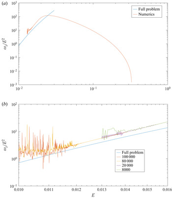
The negative sign in (3.43) corresponds to an unstable mode. Figure 8(a) shows a comparison between the asymptotic expression in (3.43) and the numerical results in an appropriate scaled form. Although, as shown in figure 8(a), the numerical results do not extend until an  $E$ small enough for a near-quantitative agreement with the analytical prediction, the numerical curve nevertheless turns around at
 $E\approx 0.02$, with there being a clear indication of an eventual convergence to the analytical asymptote.
(a) Comparison of the numerical growth rate ( $\tilde {N} = 8000$) and the analytical predictions for the full problem (see (3.43)) for
 $m$ = 2. (b) The breakdown of the numerical results at progressively smaller
 $E$ with increasing resolution (
 $\tilde {N}$) of the shooting method; here,
 $\tilde {N}$ refers to the number of mesh points used for the spatial discretization for the numerical integration in the shooting method.

As already mentioned, the emergence of the transcendentally small length scale (and the similarly small scaling for the growth rate) implies that the numerics breaks down at a slightly smaller  $E$ (
 ${\approx }0.016$) for the resolution used in figure 8(a) (
 $\tilde {N} = 8000$). Continuing the numerical curve down to smaller
 $E$ would require an exponential increase in resolution; some evidence of the modest increase in the range of validity of the numerics, even with substantial increase in resolution, is provided in figure 8(b).
4. Conclusions
In this paper, we have described a novel inertio–elastic instability of a vortex column in a dilute polymer solution. The regime analysed pertains to large Reynolds ( ${{Re}}$) and Deborah (
 ${{De}}$) numbers, involving a balance of inertia and elasticity at leading order, and the instability is governed by the elastic equivalent of the Rayleigh equation for swirling flows; momentum diffusion and relaxation of the disturbance polymeric stresses being neglected. The instability arises due to the resonant interaction of elastic shear waves made possible by the background shear in the irrotational exterior of the vortex column. The dimensionless parameter that appears in the elastic Rayleigh equation, and that governs the growth rate of the unstable mode, is the elasticity number
 $E= {{De}} (1-\beta )/{{Re}}$.
The existence of the inertio–elastic instability is first demonstrated numerically for the Rankine vortex, for finite  $E$, as a function of the azimuthal wavenumber
 $m$. A matched asymptotic expansions approach, valid for small
 $E$, helps extend the numerical results down to
 $E= 0$, and thereby shows the absence of an elasticity threshold for instability. That is to say, the Rankine vortex is unstable for any finite
 $E$ in the limit
 ${{De}}, {{Re}} \rightarrow \infty$, although the (dimensional) growth rate is transcendentally small, scaling as
 $O(\varOmega _0 {E}^2 {\rm e}^{-1/{E}^{{1}/{2}}})$ for
 $E\rightarrow 0$. Importantly, the finite-
 $E$ growth rate is not small, with a maximum of
 $O(0.1 \varOmega _0)$ (figure 4d). The numerical investigation further shows that the instability persists for smooth monotonically decreasing vorticity profiles – at least the ‘intense’ Rankine-like profiles which exhibit a rapid variation from the central rigidly rotating core to the irrotational exterior. This finding is in contrast to previous work in this regard for parallel shear flows. For instance, although the growth rate associated with the analogous inertio–elastic instability for submerged jets also appears to be transcendentally small for small
 $E$ (see figure 7 of Rallison & Hinch (Reference Rallison and Hinch1995)), the authors believed the instability to be essentially dependent on the discontinuity in the first normal stress difference profile that arises from the assumed abrupt transition of the base state jet profile to a quiescent ambient at either end (where the jet velocity equals zero – see Miller (Reference Miller2005)). Thus, the instability was speculated to be absent for smoothed versions of such jet profiles. However, the present results suggest that a slightly smoothed version of the original parabolic jet will also be subject to an analogous inertio–elastic instability. We have verified the same by analysing a smoothed version of the parabolic jet profile using a spectral calculation (not shown); an analytical approach is not possible in this case, owing to the insolubility of the inviscid (
 $E = 0$) Rayleigh equation for the plane Poiseuille profile.
An estimate of the region in the  ${{De}}$–
 ${{Re}}$ plane where one expects the shear-wave instability above to be largely unmodified may be obtained by requiring that the thickness of the viscous critical layer (assumed to be of
 $O({{Re}}^{-1/3})$ similar to the classical Newtonian case; see Drazin & Reid (Reference Drazin and Reid1981)) be much smaller than the
 $O(\sqrt {{E}}$) inviscid elastic boundary layer. This translates to the requirement
 ${{De}} \gg {{Re}}^{1/3} \gg 1$; this requirement is also consistent with the relaxation boundary layer of
 $O({{De}}^{-1})$ being asymptotically thinner than the elastic one. The elastic Rayleigh limit (
 ${{De}}/{{Re}}$ fixed,
 ${{De}}$,
 ${{Re}} \gg 1)$ is entirely consistent with this estimate. Note, however, that a large but finite
 ${{Re}}$ or
 ${{De}}$ will lead to the emergence of a weak elasticity threshold for the onset of the instability.
There is an exact analogy between the viscoelastic flows studied here, in the limit  $De \rightarrow \infty$, and MHD flows in the limit of infinite magnetic Reynolds number
 $(Re_m)$ (Ogilvie & Proctor Reference Ogilvie and Proctor2003; Ogilvie & Potter Reference Ogilvie and Potter2008; Vieu & Mutabazi Reference Vieu and Mutabazi2019); here
 $Re_m=\mu _s/(\rho \lambda _m)Re$ for a conducting fluid of density
 $\rho$, viscosity
 $\mu _s$ and magnetic diffusivity
 $\lambda _m$. Thus, the elastic shear waves examined here are the analogue of Alfvén waves in the MHD context. An analogue of the instability discussed in this paper thus likely exists in the astrophysical setting of accretion discs. In particular, accretion discs with a rapid transition in the azimuthal magnetic field would be susceptible to a Alfvén-wave resonance instability, similar to the shear-wave resonance instability described herein (Balbus & Hawley Reference Balbus and Hawley1991). Further, the matched asymptotic expansions approach involving multiple boundary layers, presented here, may be extended to gain insight into the classical non-axisymmetric magnetorotational instability (Ogilvie & Pringle Reference Ogilvie and Pringle1996; Khalzov et al. Reference Khalzov, Ilgisonis, Smolyakov and Velikhov2006) as well as MHD instabilities in parallel shear flows (Stern Reference Stern1963; Heifetz et al. Reference Heifetz, Mak, Nycander and Umurhan2015). Although a detailed comparison must await an analysis of three-dimensional perturbations, there are features associated with earlier numerical spectral calculations in the former case that bear the hallmark of a transcendentally small length scale (Ogilvie & Pringle Reference Ogilvie and Pringle1996).
In the Newtonian limit, the Rankine vortex is centrifugally stable (according to the Rayleigh criterion), and this, together with the absence of a vorticity maximum at a finite radius, implies stability to both two- and three-dimensional disturbances (Drazin & Reid Reference Drazin and Reid1981). As pointed out above, the two-dimensional inertio–elastic instability of the Rankine vortex analysed here is expected to have an MHD analogue. Further, monotonically decreasing quasi-Keplerian angular velocity profiles characterizing accretion disks are known to be susceptible to the magnetorotational instability (Ogilvie & Pringle Reference Ogilvie and Pringle1996). The MHD analogy thus implies that the Rankine vortex, and smooth Rankine-like profiles, will be susceptible to an additional inertio–elastic instability when three-dimensional perturbations, with a finite axial wavenumber, are taken into account. One expects novel features to emerge, both with regard to the CS and in terms of a denumerable infinity of discrete modes. Earlier efforts in this regard, both computations (Ogilvie & Potter Reference Ogilvie and Potter2008) and experiments (Groisman & Steinberg Reference Groisman and Steinberg1996; Boldyrev, Huynh & Pariev Reference Boldyrev, Huynh and Pariev2009; Dutcher & Muller Reference Dutcher and Muller2011, Reference Dutcher and Muller2013; Bai, Crumeyrolle & Mutabazi Reference Bai, Crumeyrolle and Mutabazi2015) have only explored the domain of existence for moderate  ${{Re}}$ and
 ${{De}}$, and for the Taylor–Couette geometry. Extending these efforts to the case of large but finite
 ${{Re}}$ and
 ${{De}}$ would help precisely delineate the domain of existence of the inertio–elastic instability.
The present inertio–elastic instability also shares similarities with the widely studied stratorotational instability, which is also postulated as a mechanism for (outward) angular momentum transport in cold weakly ionized accretion disks (Dubrulle et al. Reference Dubrulle, Marie, Normand, Richard, Hersant and Zahn2005). The latter arises from a resonance between Kelvin waves and/or inertia-gravity waves and also exhibits a transcendentally small scaling for small Rossby number (Yavneh, McWilliams & Molemaker Reference Yavneh, McWilliams and Molemaker2001; Vanneste & Yavneh Reference Vanneste and Yavneh2007). Nevertheless, there are important differences between the two cases. Most importantly, the stratorotational instability only occurs for three-dimensional perturbations. Further, the locations of the Kelvin waves are fixed in the neighbourhood of the two walls and hence the spacing between the resonating modes is fixed by the gap width; this, along with the exponential trapping of the individual waves, explains the transcendental scaling above. On the other hand, for the inertio–elastic instability, the spacing is fixed by the region where inertial and elastic stresses are of comparable magnitude (the elastic boundary layer). Finally, the eigenmode of the usual stratorotational instability does not become singular in the limit of zero growth rate (Yavneh et al. Reference Yavneh, McWilliams and Molemaker2001; Vanneste & Yavneh Reference Vanneste and Yavneh2007). The present scenario thus more closely resembles the recently studied case where the stratorotational instability results from a resonant interaction between a Kelvin/inertia-gravity wave with a baroclinic critical level (Wang & Balmforth Reference Wang and Balmforth2018).
Finally, the inertio–elastic instability examined here may be important to the general dynamics of polymeric flows at large  ${{Re}}$. Simplistically speaking, the vortex column analysed in this paper may be likened to an eddy in the turbulent cascade scenario where the time scale is short enough for elastic stresses to become comparable to inertial stresses, while at the same time being much more important than viscosity. The interaction between vortices and polymers has been shown to play a crucial role in the buffer layer structure of wall-bounded turbulent flows of dilute polymer solutions (Roy et al. Reference Roy, Morozov, van Saarloos and Larson2006; Kim et al. Reference Kim, Li, Sureshkumar, Balachandar and Adrian2007; White & Mungal Reference White and Mungal2008; Tabor & de Gennes Reference Tabor and de Gennes1986). The instability studied in this paper can be a starting point to form a deeper mechanistic understanding of the same.
Supplementary material
Supplementary material is available at https://doi.org/10.1017/jfm.2022.122.
Acknowledgments
This work has benefitted from discussions with Professor G.M. Homsy. A.R. would also like to acknowledge IIT Madras for its support of the ‘Geophysical Flows Lab’ research initiative under the Institute of Eminence framework.
Declaration of interests
The authors report no conflict of interest.