1 Introduction
The process by which a laminar boundary layer flow transitions to turbulence is of fundamental interest in fluid dynamics. For hypersonic boundary layers with streamwise curvature at small angles of attack, three kinds of instabilities, i.e. the first-mode instability, the second-mode instability and the Görtler instability, are most frequently encountered. The first-mode instability, which is analogous to the Tollmien–Schlichting waves in incompressible flows, is most unstable at oblique angles. The second-mode instability, however, is planar-component dominant. The Görtler mode is a centrifugal instability in nature and can be steady as well as unsteady with the steady instability dominating in general. While steady Görtler modes have been thoroughly investigated, unsteady Görtler vortices have been studied only recently (Boiko et al. Reference Boiko, Ivanov, Kachanov and Mischenko2010; Wu, Zhao & Luo Reference Wu, Zhao and Luo2011). The first-mode wave frequencies are generally tens of kilohertz, whereas the second-mode wave frequencies can be as high as hundreds of kilohertz. When the amplitudes of the unstable modes are large, nonlinear interactions come into play. Most investigators have focused on self-interaction (Li et al. Reference Li, Choudhari, Chang and White2010a ), K-type breakdown (Sivasubramanian & Fasel Reference Sivasubramanian and Fasel2015), subharmonic resonance (Chang & Malik Reference Chang and Malik1993; Husmeier & Fasel Reference Husmeier and Fasel2007), oblique breakdown (Franko & Lele Reference Franko and Lele2013) and secondary instabilities (Ng & Erlebacher Reference Ng and Erlebacher1992; Ren & Fu Reference Ren and Fu2015). Little attention has been paid to the interactions between the first- and second-mode instabilities or the interactions between the Görtler and second-mode instabilities. These two types of interactions are of great significance since they represent the interactions between very low-frequency and high-frequency waves and because they can provide new spectrum-fulfilling mechanisms. Maestrello, Bayliss & Krishnan (Reference Maestrello, Bayliss and Krishnan1991) numerically tracked the evolution of a planar second mode and an oblique first mode in a supersonic flat-plate boundary layer. They showed that the two-dimensional second mode significantly increased the nonlinearities and three-dimensionality of the flow field. Al-Salman (Reference Al-Salman2002) theoretically investigated the subharmonic resonance between a planar second mode and a pair of oblique first modes, and the phase-locked interactions between a planar second mode and an oblique first mode. Both cases led to super-exponential growth of the first mode. Yu & Luo (Reference Yu and Luo2014) introduced a planar second-mode wave and a pair of oblique first-mode waves at the simulation inlet in a numerical study and found that the spanwise harmonics were greatly amplified. Whang & Zhong (Reference Whang and Zhong2000) numerically studied the effects of steady Görtler vortices on the second mode. They found that stable second modes can be excited in inflectional regions formed by the Görtler vortices. Ren, Fu & Hanifi (Reference Ren, Fu and Hanifi2016) used parabolized stability equations (PSE) analyses of the evolution of first-/second-mode instabilities in the presence of finite-amplitude steady Görtler vortices to show that appropriate vortex amplitudes can stabilize both first and second modes. However, the details of the interactions between the first- and second-mode waves, as well as the interactions between the second mode and steady/unsteady Görtler vortices, are still unclear.
In experiments, nonlinear interactions between different frequencies are often identified using bicoherence. Kimmel & Kendall (Reference Kimmel and Kendall1991) used bispectral analyses to examine the nonlinear interactions in naturally occurring waves in boundary layers on straight cones in a conventional Mach 8 tunnel. They observed strong bicoherence between the low-frequency modes and the second mode. They attributed the low-frequency mode to the response of the boundary layer to ambient tunnel disturbances (see also Lachwicz, Chokani & Wikinson Reference Lachwicz, Chokani and Wikinson1996), and argued that the low-frequency waves modulated the second-mode waves with energy transfer to the second-mode sidebands. Chokani (Reference Chokani1999, Reference Chokani2005) analysed hot-wire data acquired in a Mach 6 quiet tunnel on a flared cone. The analyses showed that the harmonics resulted from phase coherent nonlinearities. Chokani concluded that the low-frequency modes arose from nonlinear interactions within limited bands of waves centred on the fundamental and harmonic waves. Shiplyuk et al. (Reference Shiplyuk, Bountin, Maslov and Chokani2003) analysed the bicoherence in a Mach 6 boundary layer on a sharp cone with naturally and artificially excited disturbances. They identified the subharmonic resonance and the interactions between the first and second modes. They also noted that the nonlinear interactions centred on the low frequencies resulted in the filling of the valleys between the spectral peaks. Hofferth et al. (Reference Hofferth, Humble, Floryan and Saric2013) combined a bicoherence analysis with focused schlieren measurements in a Mach 6 quiet tunnel on a flared cone. In addition to self-interactions of the second mode, they also observed interactions between the second mode and low-frequency disturbances. In all of these hypersonic transition experiments, the nonlinear interactions were investigated in the layer with the (approximately) maximum root-mean-square (r.m.s.) fluctuation. The bicoherence based on wall-pressure measurements measured by Munoz, Heitmann & Radespiel (Reference Munoz, Heitmann and Radespiel2014) along an inclined cone at Mach 6 also identified the interactions between the low-frequency modes (around 20 kHz) and the second mode (around 300 kHz).
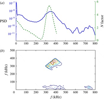
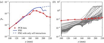
Quite recently, Zhu et al. (Reference Zhu, Zhang, Chen, Yuan, Wu, Chen, Lee and el Hak2016) (see also Zhang, Tang & Lee Reference Zhang, Tang and Lee2013; Zhang et al. Reference Zhang, Zhu, Chen, Yuan, Wu, Chen, Lee and Gad-el-Hak2015) measured wall-pressure disturbances in the quiet wind tunnel at Peking University operated with noisy conditions (referred to here as the PKU experiments). They found that the low-frequency waves (around 30 kHz) were amplified whereas the second-mode waves (around 350 kHz) were largely attenuated and vanished. The bicoherence also indicated the interactions between the low-frequency waves and the second mode in addition to the self-interactions of the second mode. However, what are the low-frequency waves? What is the mechanism beneath the interactions between the second-mode and low-frequency waves? This article is aimed at answering these questions based on theoretical and numerical tools. It should be stated at the outset that this work is not intended to completely simulate the transition process, but to find a simple yet realistic enough model to capture the relevant physical mechanism. Using linear stability analysis and parabolized stability equations (PSE), we show that the low-frequency waves likely arise from either the Görtler vortices or nonlinear forced waves from the sideband interactions of the second-mode wavepackets or the streamwise vortices driven by a pair of first-mode waves and that they interact with the second mode via the phase-locked mechanism and the subsequent parametric-resonance mechanism.
The phase-locked mechanism was proposed by Wu & Stewart (Reference Wu and Stewart1996) and Wu, Stewart & Cowley (Reference Wu, Stewart and Cowley2007) to explain the growth of broadband oblique waves in incompressible wakes and boundary layers. The phase-locked theory states that if a planar wave and a single (pair of) oblique wave(s) have (nearly) the same phase velocity, a difference mode will be generated and resonance will occur among the planar wave, the oblique wave(s) and the difference mode, which can result in rapid (super-exponential) growth of the oblique wave(s) and the difference mode. The phase-locked theory allows the three-dimensional waves to grow at different rates and to interact with the planar wave. Secondary instability theory (Herbert Reference Herbert1988) and the parametric-resonance mechanism (see a good review by Kachanov Reference Kachanov1994) also predict the growth of broadband three-dimensional waves. Instead of requiring that the phase velocities be (nearly) equal, they only require that the resonance condition (Craik Reference Craik1971) to be satisfied. However, these theories assume that the primary planar wave evolves (linearly) without interacting with the secondary waves and hence can only describe the early stage of transition.
The growth of low-frequency waves has also been seen in some direct numerical simulation (DNS) results, recently. Li, Fu & Ma (Reference Li, Fu and Ma2010c ) conducted a DNS study of boundary layer transition over a blunt cone with a small angle of attack at Mach 6. Random wall blow-and-suction perturbations were used to trigger transition. Very low-frequency waves were found rapidly amplified and distorted downstream and were believed to be ‘triggered by the upstream first or second-mode LST waves’. Sivasubramanian & Fasel (Reference Sivasubramanian and Fasel2014) performed DNS studies of the development of three-dimensional wavepackets in a sharp-cone boundary layer at Mach 6. The wavepackets were generated by pulsing the wall-normal velocity in a circular area on the cone surface with the broadband frequencies centred on the dominant frequency of the second mode. Their results indicated fundamental/subharmonic resonances as well as second-mode oblique breakdown. In addition to observing steady modes over a wide range of azimuthal wavenumbers, they also observed very low-frequency waves with frequencies far from the first-mode and second-mode waves in the disturbance spectrum. These low-frequency waves were driven by nonlinear forces since they were linearly stable. However, a detailed understanding of the evolution of the low-frequency waves and the involved nonlinear mechanism are still lacking.
Since many practical configurations involve axisymmetric bodies, the stability of such flows is important. The PKU experiments used a flared cone model composed of a straight cone and a flared afterbody. This geometry introduces the effects of transverse curvature, divergence and streamwise curvature on stability of boundary layers. The body divergence introduces a stabilizing effect (Gasperas Reference Gasperas1987) while the transverse curvature exerts a stabilizing/destabilizing influence on the axisymmetric/asymmetric disturbances (Malik & Spall Reference Malik and Spall1991). The streamwise curvature along a flared cone enhances both the first-mode and the second-mode instabilities regardless of whether the disturbances are axisymmetric or not and induces Görtler instability. The flared region also creates an adverse pressure gradient which promotes boundary layer instabilities. As a result, the stability of hypersonic boundary layers over flared cones has received much attention. Experiments similar to the PKU experiments have been undertaken with various conditions (Lachwicz et al. Reference Lachwicz, Chokani and Wikinson1996; Horvath et al. Reference Horvath, Berry, Hollis, Chang and Singer2002; Berridge et al. Reference Berridge, Chou, Ward, Steen, Gilbert, Juliano, Schneider and Gronvall2010; Hofferth et al. Reference Hofferth, Humble, Floryan and Saric2013), and DNS/PSE simulations have been used to study the fundamental breakdown (Pruett & Chang Reference Pruett and Chang1998; Laible & Fasel Reference Laible and Fasel2011; Fasel, Sivasubramanian & Laible Reference Fasel, Sivasubramanian and Laible2015; Sivasubramanian & Fasel Reference Sivasubramanian and Fasel2016), the oblique breakdown (Fasel et al. Reference Fasel, Sivasubramanian and Laible2015; Sivasubramanian & Fasel Reference Sivasubramanian and Fasel2016), the self-interaction of second-mode disturbances (Perez et al. Reference Perez, Kocian, Kuehl and Reed2012), the secondary instability (Li et al. Reference Li, Choudhari, Chang and White2010a ,Reference Li, Choudhari, Chang, Wu and Greene b ) and the receptivity (Zhong Reference Zhong2004; Balakumar & Kegerise Reference Balakumar and Kegerise2010).
This article is organized as follows. In the next section, we employ FLUENT to obtain the inviscid flow field over the flared cone used in the PKU experiments and then solve the non-similar boundary layer with spectral collocation method. In § 3, we present the formulations of linear stability theory (LST) and PSE. In § 4, LST is applied to analyse the linear instability. Nonlinear evolution of the disturbances and the involved mechanisms are then studied in detail via PSE, Floquet theory and energy transfer analysis in § 5. The numerical results are compared with the experimental data in § 6. The work is summarized in § 7.
2 Mean-flow field
An Euler/boundary layer approach (Pruett & Chang Reference Pruett and Chang1998) was used to obtain the laminar base state flow for the stability calculations. This approach is much easier to implement than direct solutions of the compressible Navier–Stokes equations and will give sufficiently accurate results. In the present study, the Euler equations were solved first in FLUENT to obtain the inviscid flow field around the flared cone. The non-similar boundary layer was then calculated using a spectral collocation method.
2.1 Inviscid flow field
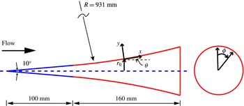
The flared cone is sketched in figure 1. This model consists of a
 $5^{\circ }$
half-angle axisymmetric sharp cone (with a nose radius of 0.05 mm) and a 160 mm-long flared afterbody located 100 mm downstream from the cone apex. The flared body was generated by a circular curve with a radius of 0.931 m. Thanks to the axisymmetric nature of the flow, the computed region can be reduced to a plane containing the axis. The flow conditions correspond to a free stream Mach number of 6, free stream pressure of 570 Pa, stagnation temperature of 433 K, and Reynolds number of
 $9.70\times 10^{6}~\text{m}^{-1}$
. In our computation, the nose radius was set to zero since the nose radius was too small to affect the stability analysis. The grid resolution was
 $1000\times 200$
in the streamwise and wall-normal directions.
Sketch of the flared-cone model and the body oriented coordinate.

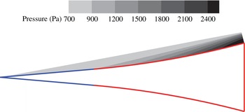
Inviscid flow field pressure contours.

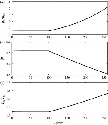
The inviscid pressure contours are shown in figure 2. A shock wave is emitted from the cone apex with a cluster of compression waves generated over the flared region. The shock wave is approximately 15 mm above the cone wall over the flared region while the boundary layer is approximately 1 mm thick. Therefore the shock wave can be disregarded when studying the boundary layer instabilities. The wall values (which are equal to the boundary layer edge values in the Euler/boundary layer approach) of the selected variables are displayed in figure 3. In the straight region, all the variables remain nearly constant, which is consistent with the contour plot in figure 2. In the flared region, the edge pressure and temperature both increase significantly, while the edge Mach number decreases nearly linearly.
Inviscid wall values versus the axial length: (a) normalized edge pressure, (b) edge Mach number, (c) normalized edge temperature.

2.2 Boundary layer flow
Consider undisturbed compressible flow past an axisymmetric body of radius
 $r_{0}(x)$
, where
 $x$
is the coordinate along the body and
 $y$
is normal to the surface. Let
 $\bar{U}$
and
 $\bar{V}$
represent the undisturbed velocity components along the
 $x$
- and
 $y$
-directions, then the boundary layer equations in the presence of a pressure gradient are
 $$\begin{eqnarray}\displaystyle & \displaystyle \bar{\unicode[STIX]{x1D70C}}\bar{U}\frac{\unicode[STIX]{x2202}\bar{U}}{\unicode[STIX]{x2202}x}+\bar{\unicode[STIX]{x1D70C}}\bar{V}\frac{\unicode[STIX]{x2202}\bar{U}}{\unicode[STIX]{x2202}y}=-\frac{\text{d}\bar{p}}{\text{d}x}+\frac{1}{r}\frac{\unicode[STIX]{x2202}}{\unicode[STIX]{x2202}y}\left(r\bar{\unicode[STIX]{x1D707}}\frac{\unicode[STIX]{x2202}\bar{U}}{\unicode[STIX]{x2202}y}\right), & \displaystyle\end{eqnarray}$$
 $$\begin{eqnarray}\displaystyle & \displaystyle \frac{\unicode[STIX]{x2202}}{\unicode[STIX]{x2202}x}(r\bar{\unicode[STIX]{x1D70C}}\bar{U})+\frac{\unicode[STIX]{x2202}}{\unicode[STIX]{x2202}y}(r\bar{\unicode[STIX]{x1D70C}}\bar{V})=0, & \displaystyle\end{eqnarray}$$
 $$\begin{eqnarray}\displaystyle & \displaystyle \bar{\unicode[STIX]{x1D70C}}\bar{c}_{p}\bar{U}\frac{\unicode[STIX]{x2202}\bar{T}}{\unicode[STIX]{x2202}x}+\bar{\unicode[STIX]{x1D70C}}\bar{c}_{p}\bar{V}\frac{\unicode[STIX]{x2202}\bar{T}}{\unicode[STIX]{x2202}y}=\frac{1}{r}\frac{\unicode[STIX]{x2202}}{\unicode[STIX]{x2202}y}\left(r\bar{k}\frac{\unicode[STIX]{x2202}\bar{T}}{\unicode[STIX]{x2202}y}\right)+\bar{\unicode[STIX]{x1D707}}\left(\frac{\unicode[STIX]{x2202}\bar{U}}{\unicode[STIX]{x2202}y}\right)^{2}+\bar{u}\frac{\text{d}\bar{p}}{\text{d}x}, & \displaystyle\end{eqnarray}$$
 $$\begin{eqnarray}\displaystyle & \displaystyle \bar{p}=\bar{\unicode[STIX]{x1D70C}}{\mathcal{R}}\bar{T}, & \displaystyle\end{eqnarray}$$
where
 $\bar{\unicode[STIX]{x1D70C}}$
is the density,
 $\bar{T}$
the temperature and
 $\bar{c_{p}}$
the specific heat. Note that a variable with an overbar denotes the undisturbed mean-flow quantity.
 ${\mathcal{R}}$
is the gas constant and
 $r$
is related to
 $r_{0}$
as
 $$\begin{eqnarray}r(x,y)=r_{0}(x)+y\cos \unicode[STIX]{x1D703},\end{eqnarray}$$
where the local value of the angle
 $\unicode[STIX]{x1D703}$
signifies the slope of the body surface. For a cylinder,
 $\unicode[STIX]{x1D703}=0$
, and for a sharp cone,
 $\unicode[STIX]{x1D703}$
is the cone half-angle. The viscosity,
 $\bar{\unicode[STIX]{x1D707}}$
, is assumed to be given by the composite relation (Mack Reference Mack1984)
 $$\begin{eqnarray}\displaystyle & \displaystyle \frac{\bar{\unicode[STIX]{x1D707}}}{\bar{\unicode[STIX]{x1D707}}_{e}}=\frac{(\bar{T}/\bar{T}_{e})^{3/2}(1+110.4/\bar{T}_{e})}{\bar{T}/\bar{T}_{e}+110.4/\bar{T}_{e}};\quad \bar{T}\geqslant 110.4~\text{K}, & \displaystyle\end{eqnarray}$$
 $$\begin{eqnarray}\displaystyle & \displaystyle \frac{\bar{\unicode[STIX]{x1D707}}}{\bar{\unicode[STIX]{x1D707}}_{e}}=\frac{\bar{T}}{\bar{T}_{e}};\quad \bar{T}<110.4~\text{K}. & \displaystyle\end{eqnarray}$$
The thermal conductivity,
 $\bar{k}$
, is prescribed so that the Prandtl number,
 $Pr$
, is equal to 0.7.
Following Malik & Spall (Reference Malik and Spall1991), we use the Mangler–Levy–Lees transformation:
 $$\begin{eqnarray}\displaystyle & \displaystyle \text{d}\unicode[STIX]{x1D709}=\bar{\unicode[STIX]{x1D70C}}_{e}\bar{\unicode[STIX]{x1D707}}_{e}\bar{U}_{e}r_{0}^{2}\,\text{d}x, & \displaystyle\end{eqnarray}$$
 $$\begin{eqnarray}\displaystyle & \displaystyle \text{d}\unicode[STIX]{x1D702}=(\bar{U}_{e}/\sqrt{2\unicode[STIX]{x1D709}})r\bar{\unicode[STIX]{x1D70C}}\,\text{d}y. & \displaystyle\end{eqnarray}$$
Define three parameters
 $F$
,
 $V$
and
 $G$
as
 $$\begin{eqnarray}\displaystyle & \displaystyle F=\bar{U}/\bar{U}_{e}, & \displaystyle\end{eqnarray}$$
 $$\begin{eqnarray}\displaystyle & \displaystyle V=\frac{2\unicode[STIX]{x1D709}}{\bar{\unicode[STIX]{x1D70C}}_{e}\bar{\unicode[STIX]{x1D707}}_{e}\bar{U}_{e}r_{0}^{2}}\left(F\frac{\unicode[STIX]{x2202}\unicode[STIX]{x1D702}}{\unicode[STIX]{x2202}x}+\frac{\bar{\unicode[STIX]{x1D70C}}\bar{V}r}{\sqrt{2\unicode[STIX]{x1D709}}}\right), & \displaystyle\end{eqnarray}$$
 $$\begin{eqnarray}\displaystyle & \displaystyle G=\bar{T}/\bar{T}_{e}. & \displaystyle\end{eqnarray}$$
Then, the governing equations in the transformed (
 $\unicode[STIX]{x1D709}$
,
 $\unicode[STIX]{x1D702}$
)-space are
 $$\begin{eqnarray}\displaystyle & \displaystyle \frac{\unicode[STIX]{x2202}}{\unicode[STIX]{x2202}\unicode[STIX]{x1D702}}\left(a_{1}\frac{\unicode[STIX]{x2202}F}{\unicode[STIX]{x2202}\unicode[STIX]{x1D702}}\right)-V\frac{\unicode[STIX]{x2202}F}{\unicode[STIX]{x2202}\unicode[STIX]{x1D702}}+a_{2}(G-F^{2})=2\unicode[STIX]{x1D709}F\frac{\unicode[STIX]{x2202}F}{\unicode[STIX]{x2202}\unicode[STIX]{x1D709}}, & \displaystyle\end{eqnarray}$$
 $$\begin{eqnarray}\displaystyle & \displaystyle \frac{\unicode[STIX]{x2202}V}{\unicode[STIX]{x2202}\unicode[STIX]{x1D702}}+F=2\unicode[STIX]{x1D709}\frac{\unicode[STIX]{x2202}F}{\unicode[STIX]{x2202}\unicode[STIX]{x1D709}}, & \displaystyle\end{eqnarray}$$
 $$\begin{eqnarray}\displaystyle & \displaystyle \frac{\unicode[STIX]{x2202}}{\unicode[STIX]{x2202}\unicode[STIX]{x1D702}}\left(a_{3}\frac{\unicode[STIX]{x2202}G}{\unicode[STIX]{x2202}\unicode[STIX]{x1D702}}\right)-V\frac{\unicode[STIX]{x2202}G}{\unicode[STIX]{x2202}\unicode[STIX]{x1D702}}+a_{4}\left(\frac{\unicode[STIX]{x2202}F}{\unicode[STIX]{x2202}\unicode[STIX]{x1D702}}\right)^{2}=2\unicode[STIX]{x1D709}F\frac{\unicode[STIX]{x2202}G}{\unicode[STIX]{x2202}\unicode[STIX]{x1D709}}, & \displaystyle\end{eqnarray}$$
where
 $$\begin{eqnarray}a_{1}=(1+\unicode[STIX]{x1D712})^{2}\frac{\bar{\unicode[STIX]{x1D70C}}\bar{\unicode[STIX]{x1D707}}}{\bar{\unicode[STIX]{x1D70C}}_{e}\bar{\unicode[STIX]{x1D707}}_{e}},\quad a_{2}=\frac{2\unicode[STIX]{x1D709}}{\bar{U}_{e}}\frac{\text{d}\bar{U}_{e}}{\text{d}\unicode[STIX]{x1D709}},\quad a_{3}=\frac{a_{1}}{Pr},\quad a_{4}=(\unicode[STIX]{x1D6FE}-1)M_{e}^{2}a_{1},\end{eqnarray}$$
and
 $\unicode[STIX]{x1D712}$
is the transverse curvature parameter
 $$\begin{eqnarray}\unicode[STIX]{x1D712}=y\cos \unicode[STIX]{x1D703}/r_{0}.\end{eqnarray}$$
The boundary conditions are
 $$\begin{eqnarray}F(0)=V(0)=\frac{\text{d}G}{\text{d}\unicode[STIX]{x1D702}}(0)=0,\quad F(\infty )=G(\infty )=1.\end{eqnarray}$$
Thus, results presented in this paper are for an adiabatic boundary condition. Since the quiet wind tunnel could operate for as long as 30 seconds (Zhang et al.
Reference Zhang, Tang and Lee2013), an adiabatic boundary condition for the wall temperature is appropriate. The flat-plate similarity solution was used as the initial profile. Numerical experiments showed that the profiles downstream are insensitive to the initial profile as the downstream position is far from the initial position. The spatial marching scheme (along
 $\unicode[STIX]{x1D709}$
-coordinate) was the Euler backward difference scheme. The discretization along the
 $\unicode[STIX]{x1D702}$
-coordinate was implemented by the Chebyshev collocation method. The resulting algebraic equations were solved with a successive iterative method (Nakamura Reference Nakamura1994), that is, the nonlinear terms were linearized first and the linear equations were then solved. This process was repeated until convergence. For example, the term
 $F_{j}^{2}$
was approximated by
 $F_{j-1}F_{j}$
, where index
 $j$
represents the iteration number. For the first iteration (
 $j=1$
),
 $F_{0}$
was given by the value of
 $F$
at last step. After solving the linear equations for
 $F_{j}$
,
 $F_{j-1}$
was updated using under-relaxation as
 $$\begin{eqnarray}F_{j-1}^{new}=sF_{j}^{new}+(1-s)F_{j-1}^{old},\quad 0<s\leqslant 1,\end{eqnarray}$$
where
 $s$
is the under-relaxation parameter. The optimal value for
 $s$
depends on the problem as well as the discretization scheme. In this paper,
 $s=0.4$
was used.
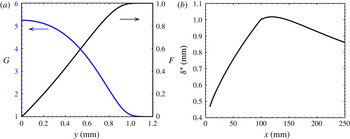
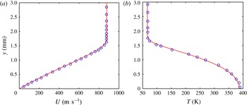
Boundary layer distributions: (a) normalized streamwise velocity and temperature at
 $x=180$
mm; (b) the boundary layer thickness (the locations of 99 %
 $\bar{U}_{e}$
). The mean flow was calculated with 250 points in the wall-normal direction.

The code validation is presented in appendix B. The wall-normal boundary layer profiles for the normalized streamwise velocity and temperature at
 $x=180$
mm are shown in figure 4(a). The velocity distribution is nearly linear across the boundary layer, which is characteristic of high-speed boundary layers. Also the frictional heating increases the wall temperature for this high-speed flow to more than five times that at the boundary layer edge. Figure 4(b) illustrates the downstream variation of the boundary layer thickness. The boundary layer thickness grows continuously along the straight region but decreases in the flared region. This was also observed by Pruett & Chang (Reference Pruett and Chang1998) and Laible & Fasel (Reference Laible and Fasel2011).
3 Stability analysis
PSE theory is suitable for investigating non-parallel effects and modal interactions up to very late in the transition process. The detailed formulation of the nonlinear PSE can be found in Bertolotti, Herbert & Spalart (Reference Bertolotti, Herbert and Spalart1992) and Chang & Malik (Reference Chang and Malik1994). Thus, only a brief introduction is given here. In the PSE formulation, the disturbance is decomposed into a rapidly varying wave-like part and a slowly varying shape function as follows
 $$\begin{eqnarray}\unicode[STIX]{x1D6F9}(x,y,\unicode[STIX]{x1D719},t)=\bar{\unicode[STIX]{x1D6F9}}(x,y)+\mathop{\sum }_{m,n}\hat{\unicode[STIX]{x1D6F9}}_{mn}(x,y)\exp \left(\text{i}\int _{0}^{x}\unicode[STIX]{x1D6FC}_{mn}\,\text{d}x-\text{i}\unicode[STIX]{x1D714}_{m}t+\text{i}n\unicode[STIX]{x1D719}\right),\end{eqnarray}$$
where
 $\unicode[STIX]{x1D6F9}\equiv (\unicode[STIX]{x1D70C},u,v,w,T)$
;
 $\bar{\unicode[STIX]{x1D6F9}}$
denotes the basic states;
 $\hat{\unicode[STIX]{x1D6F9}}_{mn}\equiv (\hat{\unicode[STIX]{x1D70C}},\hat{u} ,\hat{v},{\hat{w}},\hat{T})_{mn}$
are the shape functions for the Fourier mode (
 $m,n$
); and
 $\unicode[STIX]{x1D6FC}_{mn}$
and
 $\unicode[STIX]{x1D714}_{m}$
are the associated streamwise (complex) wavenumber and frequency. The negative imaginary part of
 $\unicode[STIX]{x1D6FC}_{mn}$
,
 $-\unicode[STIX]{x1D6FC}_{i}$
, represents the growth rate of the mode, while the real part is related to the phase velocity as
 $$\begin{eqnarray}c_{mn}\equiv \frac{\unicode[STIX]{x1D714}_{m}}{\text{Re}(\unicode[STIX]{x1D6FC}_{mn})},\end{eqnarray}$$
where
 $\text{Re}$
denotes the real part. All the variables were non-dimensionalized by the edge values of the mean flow.
 $n$
is the azimuthal wavenumber which represents the number of waves around the circumference of the cone and is related to the spanwise wavelength by
 $$\begin{eqnarray}\unicode[STIX]{x1D706}_{span}=\frac{2\unicode[STIX]{x03C0}r_{0}}{n}.\end{eqnarray}$$
The mode shape,
 $\hat{\unicode[STIX]{x1D6F9}}_{mn}(x,y)$
, is assumed to be a slowly varying function of the streamwise coordinate,
 $x$
, so that its second derivative with respect to
 $x$
is negligible. Substitute equation (3.1) into the Navier–Stokes equation and subtract the mean-flow equation to obtain the governing equations for the shape functions of each mode
 $(m,n)$
as
 $$\begin{eqnarray}({\mathcal{L}}_{0}+{\mathcal{L}}_{1})\hat{\unicode[STIX]{x1D6F9}}_{mn}+{\mathcal{L}}_{2}\frac{\unicode[STIX]{x2202}\hat{\unicode[STIX]{x1D6F9}}_{mn}}{\unicode[STIX]{x2202}x}+\frac{\text{d}\unicode[STIX]{x1D6FC}_{mn}}{\text{d}x}{\mathcal{L}}_{3}\hat{\unicode[STIX]{x1D6F9}}_{mn}={\mathcal{F}}_{mn},\end{eqnarray}$$
where
 ${\mathcal{L}}_{0}$
contains the linear-parallel terms,
 ${\mathcal{L}}_{1}$
contains the non-parallel mean-flow terms,
 ${\mathcal{L}}_{2}$
and
 ${\mathcal{L}}_{3}$
arise from the non-parallel disturbance terms, and
 ${\mathcal{F}}_{mn}$
is the nonlinear forcing term.
This system of equations is parabolic and thus requires boundary and initial conditions. The initial conditions were provided by the LST results. The boundary conditions are
 $$\begin{eqnarray}\displaystyle \hat{u} _{mn},\hat{v}_{mn},\hat{T}_{mn},{\hat{w}}_{mn}=0\quad \text{at }y=0\text{ and }\infty , & & \displaystyle\end{eqnarray}$$
which correspond to no-slip and no-temperature-fluctuation boundary conditions at the wall, and vanishing temperature and velocity disturbances as
 $y\rightarrow \infty$
. However, for the mean-flow distortion,
 $\hat{\unicode[STIX]{x1D6F9}}_{00}$
, the infinity condition for the wall-normal velocity is replaced by
 $$\begin{eqnarray}\frac{\unicode[STIX]{x2202}\hat{v}_{00}}{\unicode[STIX]{x2202}y}=0\quad \text{at}~y=\infty ,\end{eqnarray}$$
which accounts for the boundary layer growth. The boundary conditions for density were implemented by the continuity equation. Equations (3.4) were marched forward using the Euler backward scheme with the Vigneron technique used to avoid instabilities caused by the residual ellipticity (Chang & Malik Reference Chang and Malik1994).
There is still ambiguity in the
 $x$
-dependence between
 $\hat{\unicode[STIX]{x1D6F9}}_{mn}$
and
 $\unicode[STIX]{x1D6FC}_{mn}$
. In this study, the wavenumber at each station was updated as
 $$\begin{eqnarray}\unicode[STIX]{x1D6FC}^{new}=\unicode[STIX]{x1D6FC}^{old}-\text{i}\frac{1}{E}\int _{0}^{\infty }\bar{\unicode[STIX]{x1D70C}}\left(\hat{u} ^{\ast }\frac{\unicode[STIX]{x2202}\hat{u} }{\unicode[STIX]{x2202}x}+\hat{v}^{\ast }\frac{\unicode[STIX]{x2202}\hat{v}}{\unicode[STIX]{x2202}x}+{\hat{w}}^{\ast }\frac{\unicode[STIX]{x2202}{\hat{w}}}{\unicode[STIX]{x2202}x}\right)\text{d}y,\end{eqnarray}$$
where
 $$\begin{eqnarray}E\equiv \int _{0}^{\infty }\bar{\unicode[STIX]{x1D70C}}(|\hat{u} |^{2}+|\hat{v}|^{2}+|{\hat{w}}|^{2})\,\text{d}y,\end{eqnarray}$$
and the asterisk denotes the complex conjugate. This iteration continued until the largest change was less than
 $10^{-5}$
. However, equation (3.7) was not used for the mean-flow distortion (MFD) in the nonlinear-parabolized stability equations (NPSE) calculations of the hypersonic boundary layer instability in order to improve the convergence of the MFD. That means the growth or decay of the MFD was manifested simply as the growth or decay of the modulus of its shape functions rather than its wavenumber. As a result, neglecting the terms containing
 $\unicode[STIX]{x2202}^{2}\hat{\unicode[STIX]{x1D6F9}}_{mn}/\unicode[STIX]{x2202}x^{2}$
introduces additional errors of the order of
 $O(\unicode[STIX]{x1D6FC}^{2}/Re)$
. Since the wavenumber of the MFD is real with typical amplitudes of
 $O(10^{-2})$
and the Reynolds number is
 $O(10^{3})$
, this new error turns out to be about
 $O(10^{-7})$
. Recently, Zhang & Su (Reference Zhang and Su2015) argued that a more self-consistent approach is to update only the imaginary parts (oscillating part) of the wavenumbers,
 $$\begin{eqnarray}\unicode[STIX]{x1D6FC}^{new}=\unicode[STIX]{x1D6FC}^{old}+\text{Im}\left(\frac{1}{E}\int _{0}^{\infty }\bar{\unicode[STIX]{x1D70C}}\left(\hat{u} ^{\ast }\frac{\unicode[STIX]{x2202}\hat{u} }{\unicode[STIX]{x2202}x}+\hat{v}^{\ast }\frac{\unicode[STIX]{x2202}\hat{v}}{\unicode[STIX]{x2202}x}+{\hat{w}}^{\ast }\frac{\unicode[STIX]{x2202}{\hat{w}}}{\unicode[STIX]{x2202}x}\right)\,\text{d}y\right),\end{eqnarray}$$
where Im indicates the imaginary part. Equation (3.9) implicitly keeps the wavenumber of the MFD unchanged and also introduces an additional error of
 $O(10^{-7})$
for each mode. Nevertheless, Zhang & Su (Reference Zhang and Su2015) found little difference between the results using these two iteration methods.
Neglecting the nonlinear term
 ${\mathcal{F}}_{mn}$
gives the linear parabolized stability equations (LPSE) which can be used to track the evolutions of each modes separately since they are decoupled. Further neglecting the non-parallel terms yields the LST equations
 $$\begin{eqnarray}{\mathcal{L}}_{0}(y,\unicode[STIX]{x1D6FC},n,\unicode[STIX]{x1D714})\hat{\unicode[STIX]{x1D6F9}}=0.\end{eqnarray}$$
These equations with the homogenous boundary conditions (3.5) give an eigenvalue problem. For a temporal approach,
 $\unicode[STIX]{x1D6FC}$
and
 $n$
are given real values and
 $\unicode[STIX]{x1D714}$
is the unknown complex eigenvalue. For a spatial approach
 $\unicode[STIX]{x1D714}$
and
 $n$
are given real variables and
 $\unicode[STIX]{x1D6FC}$
is the unknown complex eigenvalue. The temporal eigenvalue spectrum can be solved directly using the eigenvalue solver of Matlab. However, the spatial eigenvalue equations are nonlinear with respect to
 $\unicode[STIX]{x1D6FC}$
(including
 $\unicode[STIX]{x1D6FC}^{2}$
terms), so they need to be solved iteratively starting from an initial guess or be doubled to become linear equations with the new variables
 $\tilde{\unicode[STIX]{x1D6F9}}\equiv \{\hat{\unicode[STIX]{x1D6F9}},~\unicode[STIX]{x1D6FC}\hat{\unicode[STIX]{x1D6F9}}\}$
. The operators for both approaches were discretized using the Chebyshev collocation method (global solver) as well as the compact fourth-order finite difference method (local solver) proposed by Malik (Reference Malik1990). The differences between the results from these two methods were negligible.
4 Linear instability
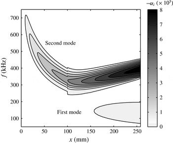
In this section we present the LST results for the PKU flared-cone model. Figure 5 shows the contours of the constant amplification rate for axisymmetric disturbances. The unstable first- and second-mode frequency bands are clearly distinguishable since they are separated by a stable region. The unstable second-mode frequency band increases over the flared region (
 $x>100$
mm) due to the decreasing boundary layer thickness. Also, the contours have discontinuities at
 $x=100$
mm due to the discontinuity in the streamwise curvature between the straight and flared regions.
Contours of the constant amplification rate
 $-\unicode[STIX]{x1D6FC}_{i}$
in the (
 $x$
–
 $f$
) plane for axisymmetric disturbances. Results generated by the LST solver.

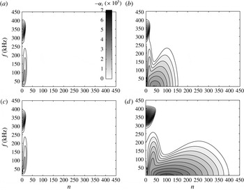
The unstable regions for oblique waves are displayed in figure 6 at various locations. At
 $x=95.2$
mm which is near the end of the straight region, the high-frequency band corresponds to the second mode with its peak at
 $n=0$
. Thus, the most unstable second-mode waves are the axisymmetric components as expected. The low-frequency band is associated with the oblique first mode centred at
 $(70,15)$
(
 $f=70$
kHz,
 $n=15$
). Once the flow has entered the flared region, at
 $x=102$
mm in figure 6(b), another broad unstable region centred at
 $(0,40)$
appears, which is the Görtler/centrifugal instability. The Görtler instability owes its existence to the streamwise curvature,
 $\unicode[STIX]{x1D705}$
, since it totally disappears for
 $\unicode[STIX]{x1D705}=0$
in the LST calculation as shown in figure 6(c). Note that the Görtler instability occurs over a large frequency range, from 0 to 230 kHz, which includes almost the entire unstable frequency range of the first mode. Farther downstream (
 $x=187.3$
mm), the spectrum broadens and spreads to higher azimuthal wavenumbers due to the decreasing wave angles of the disturbances in the downstream direction resulting from the divergence of the conical geometry. The unstable regions for the first and second modes again separate as the latter shifts to the higher-frequency region. All three instabilities have moderate increases in the amplification rates due to the adverse pressure gradient.
Contours of the constant amplification rate
 $-\unicode[STIX]{x1D6FC}_{i}$
in the (
 $n$
,
 $f$
)-plane at various positions: (a)
 $x=95.2$
mm, (b)
 $x=102$
mm, (c)
 $x=102$
mm with
 $\unicode[STIX]{x1D705}=0$
and (d)
 $x=187.3$
mm. All the plots have the same contour levels.

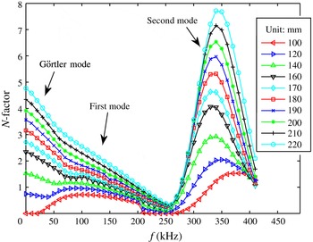
Figure 7 shows the maximum
 $N$
-factor curves versus the frequency at several locations on the flared cone. The
 $N$
-factor of an instability wave is defined as
 $$\begin{eqnarray}N(x)=\ln \left(\frac{A(x)}{A_{0}}\right),\end{eqnarray}$$
where
 $A(x)$
is the disturbance amplitude at a given downstream position,
 $x$
, and
 $A_{0}$
is the disturbance amplitude at its lower neutral point. The positions here are the same as those of the pressure sensors (PCB) in the PKU experiments. The
 $N$
-factor curves represent the amplitude distribution with frequency (see Berridge et al.
Reference Berridge, Chou, Ward, Steen, Gilbert, Juliano, Schneider and Gronvall2010). Hence, this figure sketches the linear evolution of the instability modes along the flared cone provided that all the modes have the same amplitude when they enter the amplified region. As mentioned earlier, there are at least three types of linear instabilities, i.e. the Görtler mode, the first mode and the second mode. In this figure, the Görtler mode dominates over the frequency range of (0, 50 kHz) with an azimuthal wavenumber of approximately 50, the first mode dominates over the frequency range of (50 kHz, 250 kHz) with an azimuthal wavenumber of approximately 20 and the second mode dominates over the frequency range of (250 kHz, 410 kHz). The most amplified second-mode frequency is initially at 380 kHz (
 $x=110$
mm), then shifts to 330 kHz (
 $x=160$
mm) and finally increases to about 350 kHz (
 $x=220$
mm). These frequency shifts are consistent with the variation of the boundary layer thickness as shown in figure 4.
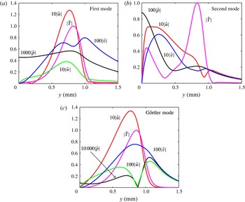
The mode shapes for the instabilities are shown in figure 8. The first and Görtler modes concentrate on the boundary layer edge (close to the generalised inflection point), whereas the main part of the second mode lies below the sonic line (at approximately
 $y=0.5$
mm) with only the maximum temperature near the boundary layer edge. The temperature disturbance has the largest amplitude while the pressure disturbance has the smallest amplitude for all three modes. The results in figure 8 also show that the relative amplitude of the pressure disturbances compared to the temperature amplitude for the second, first and Görtler modes are of the order of
 $10^{-2}$
,
 $10^{-3}$
and
 $10^{-4}$
, respectively. The pressures at the wall for the last two modes are even smaller. As a result, the first mode and the Görtler mode are more difficult to detect via wall-pressure sensors than the second mode.
5 Weakly nonlinear development
In this section we utilize NPSE to investigate the two types of nonlinear interactions indicated by the experiments (Zhu et al. Reference Zhu, Zhang, Chen, Yuan, Wu, Chen, Lee and el Hak2016), that is, the self-interaction of the second mode and the interactions between the second-mode waves and the low-frequency waves. The second type can occur in two possible ways. Either, the dominant second mode interacts with its sideband to generate low-frequency difference waves, which has been studied by Dong & Luo (Reference Dong and Luo2007) in a hypersonic sharp-cone boundary layer transition simulation or the dominant second mode interacts with the oblique low-frequency wave, generating the high-frequency difference and sum modes, which have also been investigated by some researchers (Maestrello et al. Reference Maestrello, Bayliss and Krishnan1991; Al-Salman Reference Al-Salman2002; Yu & Luo Reference Yu and Luo2014). Here we only focus on the latter, the reason for which will become apparent later. This interaction can be further divided into two cases. Case I is concerned with the interactions between a second-mode wave and an oblique low-frequency mode, while case II is concerned with the interactions between a second-mode wave and a pair of oblique low-frequency modes which propagate at equal angles but in opposite directions with respect to the mean flow. It should be noted that these two cases are only model interactions and that case II is more realistic compared to case I.
 $N$
-factors (maximum values with respect to the azimuthal wavenumber) at various locations. The LST ware calculated with 50 grid points which was found to be enough for the desired accuracy.

Comparison of disturbance profiles of different modes: (a) the first mode (60 kHz,
 $n=30$
); (b) the second mode (350 kHz,
 $n=0$
); (c) the Görtler mode (0 kHz,
 $n=90$
). The mode shapes were normalized by the temperature amplitude.

5.1 Parametric study
In these calculations, mode (
 $f_{2nd},0$
) (
 $f_{2nd}=350$
kHz,
 $n=0$
) was chosen to represent the second-mode waves, since it is one of the most amplified components and has a frequency close to the measured peak in the PKU experiments, as shown in § 6. The low-frequency disturbances, however, were more difficult to identify in the PSE simulations because the unstable regions in the
 $n$
–
 $f$
plane for low-frequency disturbances (including the Görtler mode and the first mode) are much larger than the second-mode instability region, and the azimuthal wavenumber could not be measured in the PKU experiments. Thus, a parametric study was performed first to clarify the effects of the frequency and azimuthal wavenumber. This subsection considers the case I interactions with the case II interactions discussed in § 5.4.
Spectra of the initially seeded oblique waves at
 $x=180$
mm: (a) contours of the linear amplitudes
 $\ln A_{lin}/A_{0}$
with a level step of 0.5; (b) contours of the nonlinear amplitudes
 $\ln A_{non}/A_{0}$
with a level step of 1; (c) contours of the ratios of the nonlinear amplitudes to the linear amplitudes
 $\ln A_{non}/A_{lin}$
with a level step of 0.5.

The second-mode wave (
 $f_{2nd}$
, 0) and a low-frequency wave
 $(f_{low},n)$
were initially seeded in each PSE simulation. The main interactions can be summarized as
 $$\begin{eqnarray}\displaystyle & \displaystyle (f_{2nd},0)-(f_{low},n)\rightarrow (f_{2nd}-f_{low},-n); & \displaystyle\end{eqnarray}$$
 $$\begin{eqnarray}\displaystyle & (f_{2nd},0)+(f_{low},n)\rightarrow (f_{2nd}+f_{low},n); & \displaystyle\end{eqnarray}$$
 $$\begin{eqnarray}\displaystyle & (f_{2nd}+f_{low},n)+(f_{2nd}-f_{low},-n)\rightarrow (2f_{2nd},0); & \displaystyle\end{eqnarray}$$
 $$\begin{eqnarray}\displaystyle & (f_{2nd},0)+(f_{2nd},0)\rightarrow (2f_{2nd},0). & \displaystyle\end{eqnarray}$$
The interactions with the MFD are not shown here but were considered in the PSE simulations. Only six modes, i.e. the second mode, its first harmonic, MFD, the low-frequency mode, the difference mode and the sum mode, were considered in each PSE simulation. Such a simple model turns out to suffice for the parametric study.
Typical amplitude evolution in the four regions: (a) mode
 $(140,50)$
in region
 $A$
, (b) mode
 $(10,50)$
in region
 $B$
, (c) mode
 $(60,10)$
in region
 $C$
and (d) mode
 $(30,50)$
in region
 $D$
. The dashed lines correspond to linear evolutions.

A total of 1258 cases, covering 34 frequencies and 37 azimuthal wavenumbers, were calculated. Two of these cases,
 $(0,10)$
and
 $(5,10)$
, failed to converge before the last breakdown and are therefore disregarded here. The second and low-frequency modes were seeded at
 $x=100$
mm (the beginning of the flare region) with initial amplitudes equivalent to the r.m.s. temperature fluctuations of 5 % and 0.01 %. The initial second-mode amplitude was chosen such that the second mode became saturated at approximately
 $x=170$
mm as observed in the experiments (see figure 27). Different initial oblique-wave amplitudes may change the breakdown positions of the PSE simulations but do not seem to alter the basic evolution process. The contours of the low-frequency wave amplitudes in the
 $n$
–
 $f$
plane are shown in figure 9 for a streamwise location of
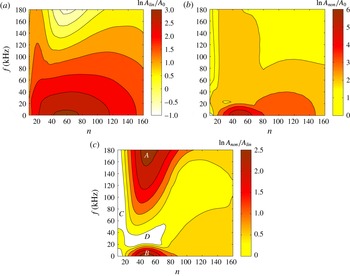
 $x=180$
mm. The linear distribution is shown in figure 9(a). As expected, the amplitudes of the unstable first and Görtler modes increase while those of the stable modes decrease. The amplitude spectrum in the nonlinear case is illustrated in figure 9(b). The low-frequency modes are all amplified from the initial amplitude. The most amplified ones are the low-frequency Görtler modes (
 $f<20$
kHz and
 $20<n<80$
at
 $x=180$
mm) for which breakdowns of the PSE simulations occur first.
Amplitude and phase-velocity evolution of low-frequency waves with a fixed azimuthal wavenumber and different frequencies (a,c) and a fixed frequency and different azimuthal wavenumbers (b,d).

The contours of the amplitude ratios defined as
 $\ln A_{non}/A_{lin}$
are shown in figure 9(c) to further clarify the effects of the second mode on the evolution of the oblique waves. If the amplitude ratio is negative (the white space in the figure), then the second mode suppresses the low-frequency mode. Otherwise, the second mode plays a positive role. The results show that most of the modes are amplified compared to the linear case, of which two regions,
 $A$
and
 $B$
, are most prominent. Region
 $A$
essentially consists of linear stable modes. The large amplitude ratios in that region are mainly due to the small linear amplitudes. The attenuated modes lie in regions,
 $C$
and
 $D$
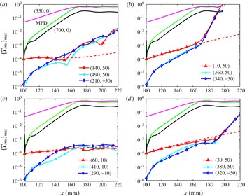
. Figure 10 shows the typical amplitude evolutions of the modes in these four regions. The selected modes are
 $(140,50)$
,
 $(10,50)$
,
 $(60,10)$
and
 $(30,50)$
from region
 $A$
,
 $B$
,
 $C$
and
 $D$
, respectively. It shows that all these four modes evolve linearly at first, and then interact with their difference/sum modes as well as the second mode. In the latter stage, these four modes behave quite differently which results in different characteristics of these regions. Mode
 $(140,50)$
exhibits large oscillations, although it still grows moderately. Mode
 $(10,50)$
is strongly amplified at a nearly constant rate. Mode
 $(60,10)$
remains saturated. Mode
 $(30,50)$
is slightly attenuated for a long distance and then amplified like mode
 $(10,50)$
, which implies that region
 $D$
may eventually be incorporated into region
 $B$
. Moreover, mode
 $(10,50)$
and mode
 $(30,50)$
have the same amplification rates as the difference/sum modes, which suggests that these oblique waves are in resonance. This resonance is explored in detail based on Floquet theory in the next subsection.
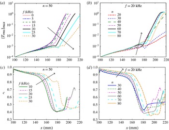
The amplitude and phase-velocity evolution of the low-frequency waves in region
 $B$
are shown in figure 11 for various frequencies and azimuthal wavenumbers. The phase velocities slowly decrease during the linear stage, sharply drop from approximately 0.9 to approximately 0.4 before the resonant growth begins with a slow growth section followed by a rapid increase. For a fixed azimuthal wavenumber the length of the linear stage increases with the frequency while the growth rate in the resonance stage decreases with the frequency. This observation implies that region
 $B$
will broaden at higher frequencies. Modes with shorter linear stages and stronger resonance stages have earlier breakdowns of the simulation. For a fixed frequency, the mode with an azimuthal wavenumber of 50 is the first to induce breakdown of the simulation. Meanwhile, modes with larger azimuthal wavenumbers have lower phase velocities at the resonance stage.
Of all the cases considered in the parametric study, two groups are of particular interest. One is the steady waves. The interaction between this group and the second mode is indeed a fundamental resonance. The present results show that the fundamental resonance is a dominant interaction, which is consistent with the findings of Sivasubramanian & Fasel (Reference Sivasubramanian and Fasel2014). They modelled and investigated a natural transition scenario using wavepackets and then investigated the fundamental resonance in detail in Sivasubramanian & Fasel (Reference Sivasubramanian and Fasel2015). The other is the subharmonic waves with half the second-mode frequency (175 kHz). The interaction between this group and the second mode corresponds to a subharmonic-resonance type. However, the present work indicates that the subharmonic resonance is weak in a hypersonic boundary layer, as was also observed by Husmeier & Fasel (Reference Husmeier and Fasel2007) and Sivasubramanian & Fasel (Reference Sivasubramanian and Fasel2014).
5.2 Floquet analysis
This subsection shows that Floquet theory can well describe the resonance stage and explain the selection mechanism observed in the parametric study in § 5.1. The details of Floquet theory and its application to secondary instability studies can be found in Herbert (Reference Herbert1988) and Ng & Erlebacher (Reference Ng and Erlebacher1992). In the parametric-resonance stage in this case, the base flow is the undisturbed laminar flow plus the second mode, the MFD and the harmonics as
 $$\begin{eqnarray}\bar{\unicode[STIX]{x1D6F9}}=\bar{\unicode[STIX]{x1D6F9}}_{0}+{\mathcal{A}}_{2nd}\hat{\unicode[STIX]{x1D6F9}}_{2nd}(x,y)\text{e}^{\text{i}\unicode[STIX]{x1D6FC}x-\text{i}\unicode[STIX]{x1D714}t}+{\mathcal{A}}_{M}\hat{\unicode[STIX]{x1D6F9}}_{M}(x,y)+\text{harmonics}+\text{c.c.},\end{eqnarray}$$
where
 $\unicode[STIX]{x1D6FC}$
and
 $\unicode[STIX]{x1D714}$
are the wavenumber and the circular frequency of the second-mode wave.
According to Floquet theory, the periodic base flow given by equation (5.5) can support three-dimensional disturbances for a given azimuthal wavenumber,
 $n$
, as follows:
 $$\begin{eqnarray}\unicode[STIX]{x1D6F9}_{s}=\unicode[STIX]{x1D716}\text{e}^{\unicode[STIX]{x1D6FE}x}\text{e}^{\text{i}n\unicode[STIX]{x1D719}}\text{e}^{\unicode[STIX]{x1D70E}_{d}(\text{i}\unicode[STIX]{x1D6FC}x-\text{i}\unicode[STIX]{x1D714}t)}\mathop{\sum }_{m=-\infty }^{\infty }\hat{\unicode[STIX]{x1D6F9}}_{m}(y)\text{e}^{m(\text{i}\unicode[STIX]{x1D6FC}x-\text{i}\unicode[STIX]{x1D714}t)}+\text{c.c.},\end{eqnarray}$$
where
 $\unicode[STIX]{x1D6FE}$
is the characteristic exponent and
 $\unicode[STIX]{x1D70E}_{d}$
is a detuning parameter that distinguishes the various types of secondary instabilities. The fundamental resonance corresponds to
 $\unicode[STIX]{x1D70E}_{d}=0$
. The subharmonic resonance is associated with the case of
 $\unicode[STIX]{x1D70E}_{d}=0.5$
. For
 $0<\unicode[STIX]{x1D70E}_{d}<0.5$
, the secondary waves are called combination resonance modes (or detuned modes). When
 $\unicode[STIX]{x1D6FE}$
is real, the secondary and primary disturbances travel with the same phase velocity in the downstream direction, i.e. they are phase locked. For complex
 $\unicode[STIX]{x1D6FE}=\unicode[STIX]{x1D6FE}_{r}+i\unicode[STIX]{x1D6FE}_{i}$
, the phase velocities of the two disturbances differ. Practical calculations only need to retain three terms in the solution to (5.6) as
 $$\begin{eqnarray}\unicode[STIX]{x1D6F9}_{s}=\unicode[STIX]{x1D716}\text{e}^{\unicode[STIX]{x1D6FE}x}\text{e}^{\text{i}n\unicode[STIX]{x1D719}}\text{e}^{\unicode[STIX]{x1D70E}_{d}(\text{i}\unicode[STIX]{x1D6FC}x-\text{i}\unicode[STIX]{x1D714}t)}(\hat{\unicode[STIX]{x1D6F9}}_{-1}(y)\text{e}^{-(\text{i}\unicode[STIX]{x1D6FC}x-\text{i}\unicode[STIX]{x1D714}t)}+\hat{\unicode[STIX]{x1D6F9}}_{0}(y)+\hat{\unicode[STIX]{x1D6F9}}_{1}(y)\text{e}^{\text{i}\unicode[STIX]{x1D6FC}x-\text{i}\unicode[STIX]{x1D714}t})+\text{c.c.},\end{eqnarray}$$
where these three terms are analogous to the difference, low-frequency and sum modes in our case, respectively.
Substituting equations (5.5) and (5.7) into the Navier–Stokes equations, neglecting the non-parallel effects and the terms of
 $O({\mathcal{A}}^{2}),O(\unicode[STIX]{x1D716}^{2})$
and higher orders give a complex eigenvalue problem of the form
 $$\begin{eqnarray}{\mathcal{M}}\unicode[STIX]{x1D701}=0,\end{eqnarray}$$
where
 ${\mathcal{M}}$
is a function of the base flow alone and
 $\unicode[STIX]{x1D701}$
is the vector of unknown variables
 $\hat{\unicode[STIX]{x1D6F9}}_{j}$
(
 $j=-1,0,1$
). This equation along with the boundary conditions in (3.5) was solved using the same numerical methods as for the LST problem.
Growth rates (a) and phase velocities (b) of the low-frequency modes at
 $x=180$
mm predicted by Floquet theory.

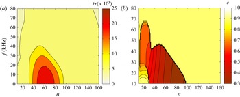
Figure 12 shows the contours of the growth rates and phase velocities, predicted by Floquet theory, of the low-frequency waves at
 $x=180$
mm. This figure was plotted based on the most unstable eigenvalue from each of 7326 cases. The region with the large growth rates (
 $\unicode[STIX]{x1D6FE}_{r}>0.01$
) approximately coincides with regions
 $B$
and
 $D$
in figure 9(c). Note that Floquet theory only predicts the growth rates when the modes are in resonance, whereas in PSE simulations, the modes need to evolve to reach the resonant states. As shown by the parametric study in § 5.1, higher-frequency modes will start to grow farther downstream due to resonance. This is why region
 $D$
in figure 9(c) does not show any amplification.
The corresponding phase velocities, however, exhibit a peculiar distribution. One can observe that a polygonal line divides the contours into two regions. On the right side, the phase velocities are nearly the same as that of the second mode (around 0.9). On the left side, except for the lower-left corner, however, the phase velocities decrease with the azimuthal wavenumber, which is consistent with the observations in figure 11(d).
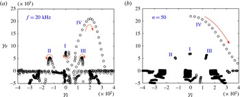
The reason for this distribution of the phase velocities can be found by a close examination of the eigenvalue spectrum. Figure 13(a,b) shows the eigenvalue spectra for various azimuthal wavenumbers and for various frequencies. For a given set of parameters, there are in general four unstable modes as labelled in the figure. Mode I lies approximately on the real axis with modes II and III almost symmetrical around mode I. Mode IV is in the upper-right quadrant.
Eigenvalue spectra at
 $x=190$
mm predicted by the secondary instability calculation for a fixed frequency (20 kHz) with the azimuthal wavenumber varying from 10 to 120 by steps of 5 (a), and for the cases when the azimuthal wavenumber is fixed (50) with the frequency varying from 0 to 80 by steps of 4 (b). The arrows indicate the trajectory directions.

For a fixed frequency, mode IV moves along a nearly quadratic curve, reaching a peak at approximately
 $n=60$
and then going down until becoming part of the continuous spectrum. Mode II (III) first moves upwards to the left (right), reaches a peak, and then moves downwards. The motion of mode I is quite complex as it first moves upwards, then downwards, then upwards again, and finally downwards. Note that, as with mode IV, the first three modes will all become stable for very large azimuthal wavenumbers. For a fixed azimuthal wavenumber, modes I, II and III change little with the frequency, which indicates that these three modes depend essentially on the azimuthal wavenumber rather than the frequency. Mode IV, however, initially lies on the real axis (representing a fundamental resonance), then moves towards the lower-right side and eventually merges with the continuous spectrum.
These mode shifts change the imaginary part of the dominant eigenvalue, and, thus, the phase velocities of the secondary waves. Therefore, the peculiar distribution of the phase velocity can be explained as follows. For a fixed frequency and quite small azimuthal wavenumbers, mode I prevails and the phase velocity is close to that of the second-mode wave, changing slightly with the azimuthal wavenumber. As the azimuthal wavenumber increases so that mode IV becomes the most unstable mode, the phase velocity starts to decrease due to the increasing imaginary part of the eigenvalue. Finally, mode I again becomes the most unstable mode, causing a jump in the phase velocity. For a fixed azimuthal wavenumber and low frequencies, mode IV dominates. Although the imaginary part increases as mode IV moves, the streamwise wavenumber also increases, with the combined effects resulting in a slightly varying phase velocity. However, the phase velocity still jumps when the dominant mode changes from mode IV to mode I at a critical frequency. Since the phase velocity may jump with both increasing azimuthal wavenumber and increasing frequency, the polygonal line edge between the high and low phase velocity is reasonable and may not turn to a smooth curve by increasing the number of cases calculated. Nevertheless, in spectra close to the edges these four modes usually have comparable growth rates and, hence, have nearly equivalent contributions to the disturbances in the PSE simulations. Therefore, the phase velocities predicted by the PSE simulations will change gradually across the edge (not shown here).
5.3 Interaction between a second-mode wave and an oblique low-frequency wave
The
 $(20,50)$
mode was used here as a representative single low-frequency mode to study in detail. The evolution of the
 $(20,50)$
mode captures all the essential features of the most amplified low-frequency modes as shown in figure 11. In addition, this mode frequency is above the cutoff frequency of the PCB sensors, so it is likely detected in experiments. Finally, this mode lies in the Görtler instability region and is, thus, an unsteady Görtler mode. Thus, we refer to this mode as the Görtler mode in this subsection, although the streamwise curvature plays a secondary role in such interactions as will be shown later.
Here, the number of grid points along the wall-normal direction was increased to 151. The initial settlings were the same as those in the parametric study with the initial amplitude of the Görtler mode increased to 0.1 % to induce earlier breakdown. Four modes, the MFD, the difference mode
 $(f_{2nd}-f_{low},-n)$
, the sum mode
 $(f_{2nd}+f_{low},n)$
and the harmonic
 $(2f_{2nd},0)$
were directly triggered via nonlinear interactions. These four modes along with the two seeded modes will generate higher-order modes, in which nine modes were included here:
 $(3f_{2nd},0)$
,
 $(4f_{2nd},0)$
,
 $(2f_{low},2n)$
,
 $(2f_{2nd}+f_{low},n)$
,
 $(2f_{2nd}-f_{low},-n)$
,
 $(2f_{2nd}+2f_{low},2n)$
,
 $(2f_{2nd}-2f_{low},-2n)$
,
 $(f_{2nd}-2f_{low},-2n)$
and
 $(f_{2nd}+2f_{low},2n)$
.
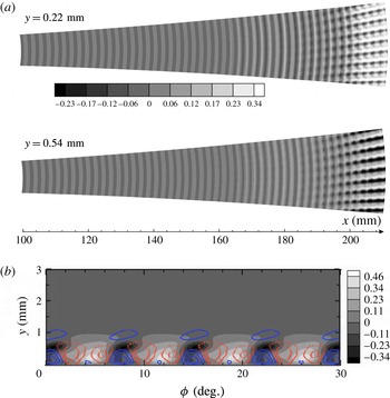
Contours of the streamwise velocity disturbances normalized by the boundary layer edge velocity at
 $x=100$
mm: (a) in the
 $x$
–
 $\unicode[STIX]{x1D719}$
planes with
 $y=0.22$
mm (
 ${\approx}0.2\unicode[STIX]{x1D6FF}^{\ast }$
) and
 $y=0.54$
mm (
 ${\approx}0.5\unicode[STIX]{x1D6FF}^{\ast }$
); (b) in the
 $y$
–
 $\unicode[STIX]{x1D719}$
plane with
 $x=200$
mm. Part (b) also shows the vertical velocity contours with the dashed lines representing negative values. The level step is 0.023 (20
 $\text{m}~\text{s}^{-1}$
).

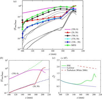
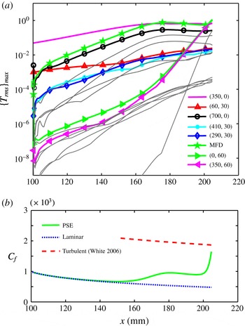
(a) Streamwise development of the maximum temperature disturbance amplitude. (b) Comparison of the linear case (dashed lines) with the nonlinear evolution of the second mode with only self-interaction (dotted line). (c) Time- and azimuthal-averaged skin friction coefficient.

Figure 14(a) shows contours of the instantaneous streamwise velocity disturbances (normalized by the boundary layer edge velocity at
 $x=100$
mm) in planes at constant distances from the wall. In the upstream region, the flow structures are essentially two-dimensional, which corresponds to the large-amplitude second mode initially forced onto the flow. Farther downstream, the two-dimensional structures become more prominent due to the growth of the second mode. Later, three-dimensional ripples appear and eventually evolve into oblique high- and low-speed streak-like structures. These streak-like structures have the same spanwise wavelength as the Görtler mode regardless of whatever smaller structures are inside, which shows that the Görtler wave is dominant. Streamwise (temperature) streaks were also recently observed for a similar flared-cone model in experiments by Berridge et al. (Reference Berridge, Chou, Ward, Steen, Gilbert, Juliano, Schneider and Gronvall2010). Direct numerical simulations by Sivasubramanian & Fasel (Reference Sivasubramanian and Fasel2015, Reference Sivasubramanian and Fasel2016) showed that both the second-mode fundamental breakdown and the oblique breakdown may be responsible for these streaks. Their DNS results showed only steady streamwise streaks. The present work, however, shows that unsteady streamwise streaks are also likely to arise. The details of the streak-like structures are illustrated in the slice at
 $x=200$
mm shown in figure 14(b). Vertical velocity disturbance contours are also shown with the dashed lines representing negative values. The low- and high-speed regions can be seen with the low-speed peaks at slightly higher positions than the high-speed peaks. Their positions coincide with the edges between the positive and negative contour lines of the vertical velocities, implying that the low and high-speed structures are associated with the vertical velocities, that is, positive vertical velocities (upwash) transfer low momentum fluid to high momentum regions resulting in velocity defects in the high momentum regions, and vice versa.
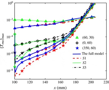
Of the five primary variables, the temperature disturbances are dominant and are found to be the most suitable for tracking the mode evolutions. Figure 15(a) illustrates the evolution of
 $|\hat{T}_{rms}|_{max}$
versus axis position for the six primary modes and higher-order modes (grey lines). The PSE calculation breaks down at approximately
 $x=210$
mm, indicating the occurrence of transition. The main feature of the interactions between the second mode and the Görtler mode can be clearly seen by comparing the nonlinear evolution with the linear as well as the self-interaction cases in figure 15(b). This figure shows that the second mode grows fast to high amplitudes, and then becomes saturated due to self-interaction. During the saturation stage of the second mode, the Görtler mode is strongly amplified. Finally, the second mode begins to decay and the rapid growth of the Görtler mode ends. Such rapid decay of the second mode was also observed by Sivasubramanian & Fasel (Reference Sivasubramanian and Fasel2015) for fundamental breakdown transition of a boundary layer over a sharp cone and by Fasel et al. (Reference Fasel, Sivasubramanian and Laible2015) over a flared cone. Li et al. (Reference Li, Choudhari, Chang and White2010a
) considered only the self-interactions of the second mode along a compression cone and also observed the rapid decay of the second mode. However, in the present investigation the rapid decay of the second mode is caused by the interactions with other modes, as shown in figure 15(b), instead of self-interactions. This difference may result from the different flow conditions and geometric models. The work of Li et al. (Reference Li, Choudhari, Chang and White2010a
) implied that if the PKU model were much longer, the rapid decay of the second mode could also be observed in the PSE simulations including only self-interactions.
The downstream development of the temporally and azimuthally averaged skin friction coefficient,
 $C_{f}$
, is shown in figure 15(c). The skin friction coefficient was calculated as
 $$\begin{eqnarray}C_{f}=\frac{2\bar{\unicode[STIX]{x1D707}}(\unicode[STIX]{x2202}\bar{u}/\unicode[STIX]{x2202}y)|_{y=0}}{Re}.\end{eqnarray}$$
The skin friction coefficient curve obtained from the simulations is compared with a turbulent boundary layer correlation from White (Reference White2006, p. 558). The skin friction coefficient plotted in figure 15(c) initially follows the laminar curve up to 140 mm, then slightly increases until it slowly decays again. Beyond 190 mm, the curve rises steeply, reaches a peak at
 $x=200$
mm and then drops sharply. The initial deviation of the skin friction coefficient from its laminar value, well before the final transition, is due to the large amplitude of the MFD which is driven by the growing second-mode wave. Similar phenomenon has also been reported by Franko & Lele (Reference Franko and Lele2013) and Sivasubramanian & Fasel (Reference Sivasubramanian and Fasel2015). The skin friction coefficient starts to decay again as the second-mode wave becomes saturated. The second sharp rise is induced by the highly amplified Görtler mode which in turn causes the MFD to increase again. The reason for the final drop is yet unclear, and may be caused by either strong nonlinear interactions or the PSE becoming invalid at this stage.
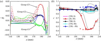
Figure 16(a) shows the growth rates against the downstream distance. After rapid changes near the inlet, the nonlinearly generated modes have much higher growth rates than the second mode and the Görtler mode up to
 $x=160$
mm. For
 $x>160$
mm, the disturbances gradually form three groups (denoted by
 $G1$
,
 $G2$
and
 $G3$
).
 $G1$
consists of the second mode, MFD and the harmonics.
 $G2$
consists of the Görtler mode, the difference/sum modes and the
 $(2f_{2nd}+f_{low},n)$
and
 $(2f_{2nd}-f_{low},-n)$
modes. The other modes form
 $G3$
. The
 $G1$
growth rates decay and become negative, whereas the
 $G2$
and
 $G3$
growth rates increase and eventually all become equal at their maximums at
 $x=180$
mm. Since the
 $G3$
modes are driven by the quadratic interactions of the
 $G2$
modes, the
 $G3$
-mode growth rates are nearly twice the
 $G2$
-mode growth rates. The good agreement with the Floquet analysis results indicates that the
 $G2$
modes start to resonate with the
 $G1$
modes. For
 $190<x<200$
mm, the
 $G2$
- and
 $G3$
-mode growth rates rapidly decay whereas the growth rates of the
 $G1$
harmonics increase again due to interactions with the
 $G2$
and
 $G3$
modes. Farther downstream, the growth rates of all the modes become comparable and rapidly oscillate, indicating full interactions between these modes.
The phase velocities for each mode are plotted in figure 16(b). The phase velocities vary by less than 5 % through most of the linear stage (from 110 mm to 150 mm). Thus, phase-locked theory can be readily applied in this region. For
 $x>150$
mm, however, the
 $(20,50)$
mode phase velocity drops sharply from approximately 0.9 to approximately 0.4 (which means that the wavelength is cut in half) at 180 mm, then slightly increases to about 0.5 at
 $x=190$
mm, and finally rapidly increases to 0.7 at the breakdown point. On the other hand, the
 $(330,-50)/(370,50)$
phase velocity increases/decreases from approximately 0.9 at approximately 160 mm to approximately
 $0.95/0.85$
at 180 mm and then remains nearly constant downstream before the breakdown point. Consequently, the relative differences between the phase velocities become as large as 100 % for
 $x>180$
mm, which indicates that phase-locked theory may not be valid there. Comparisons with the Floquet theory predictions in figure 16 demonstrate that such rapid changes in the phase velocities are due to the transition from non-resonance to a resonant state.
(a) Streamwise growth rates for different modes. The thick lines in groups
 $G1$
and
 $G2$
represent the growth rates of the second mode and the Görtler mode. (b) Phase velocities for different modes. The velocities were all normalized by the boundary layer edge velocity at
 $x=100$
mm. The stars represent the Floquet analysis results.

Comparison of the mode shapes obtained by Floquet theory (solid lines) and the mode shapes obtained by the nonlinear PSE calculation (dashed lines).

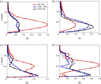
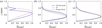
In addition to the growth rates and phase velocities, the mode shapes in the parametric-resonance stage also show very good agreement with the Floquet theory predictions as illustrated in figure 17. The minor differences may be due to non-parallel effects and nonlinear interactions with the higher-order modes. Thus, we can conclude that the parametric-resonance stage is governed by the secondary instability and can be well described by Floquet theory. Moreover, the agreement between the PSE and Floquet results verifies the applicability of these two different methods.
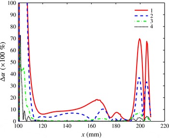
Downstream evolution of the wavenumber differences for various interactions: 1,
 $|\unicode[STIX]{x1D6FC}_{(330,-50)}+\unicode[STIX]{x1D6FC}_{(20,50)}-\unicode[STIX]{x1D6FC}_{(350,0)}|/\unicode[STIX]{x1D6FC}_{(20,50)}$
; 2,
 $|\unicode[STIX]{x1D6FC}_{(20,50)}+\unicode[STIX]{x1D6FC}_{(350,0)}-\unicode[STIX]{x1D6FC}_{(370,50)}|/\unicode[STIX]{x1D6FC}_{(20,50)}$
; 3,
 $|\unicode[STIX]{x1D6FC}_{(370,50)}+\unicode[STIX]{x1D6FC}_{(330,-50)}-\unicode[STIX]{x1D6FC}_{(700,0)}|/\unicode[STIX]{x1D6FC}_{(330,-50)}$
; 4,
 $|2\unicode[STIX]{x1D6FC}_{(350,0)}-\unicode[STIX]{x1D6FC}_{(700,0)}|/\unicode[STIX]{x1D6FC}_{(350,0)}$
.

A perfect triadic resonance should satisfy the resonance conditions (Craik Reference Craik1971)
 $$\begin{eqnarray}\unicode[STIX]{x1D6FC}_{1}+\unicode[STIX]{x1D6FC}_{2}=\unicode[STIX]{x1D6FC}_{3},\quad f_{1}+f_{2}=f_{3},\quad n_{1}+n_{2}=n_{3},\end{eqnarray}$$
which are the implicit assumptions of Floquet theory. The resonance intensities of the interactions (5.1)–(5.4) in the PSE simulations are shown in figure 18 in terms of the downstream evolution of the wavenumber differences,
 $\unicode[STIX]{x0394}\unicode[STIX]{x1D6FC}$
, among the resonant triads. The wavenumber difference for a resonant triad was defined as
 $$\begin{eqnarray}\unicode[STIX]{x0394}\unicode[STIX]{x1D6FC}\equiv \frac{|\unicode[STIX]{x1D6FC}_{1r}+\unicode[STIX]{x1D6FC}_{2r}-\unicode[STIX]{x1D6FC}_{3r}|}{\unicode[STIX]{x1D6FC}_{min}},\end{eqnarray}$$
where
 $\unicode[STIX]{x1D6FC}_{min}$
is the minimum of the real parts of the three wavenumbers and the subscript
 $r$
denotes the real part of the wavenumber. Choudhari, Chang & Jiang (Reference Choudhari, Chang and Jiang2005) defined a similar factor to represent the intensity of a triadic interaction. As the last two conditions of the resonance conditions in (5.10) are automatically satisfied in our PSE simulations, the wavenumber condition is, therefore, a measure of the resonance intensity with a smaller wavenumber difference indicating higher resonance intensity. If the disturbances have the same wave speed, then they are phase locked and in the exact resonance,
 $\unicode[STIX]{x0394}\unicode[STIX]{x1D6FC}=0$
. However, exact resonance does not necessarily require matching of the phase speeds except for the fundamental and subharmonic resonances. From figure 18, one can observe that after a short transient behaviour all the wavenumber differences fall to low levels. In the region of
 $110<x<150$
mm, the wavenumber differences for the first two interactions,
 $\unicode[STIX]{x0394}\unicode[STIX]{x1D6FC}_{1,2}$
, remain at about 10 % while the others are less than 2 %. The large values of
 $\unicode[STIX]{x0394}\unicode[STIX]{x1D6FC}_{1,2}$
are due to the small value of the denominator
 $\unicode[STIX]{x1D6FC}_{(20,50)}$
which is about a tenth of the wavenumbers of the other modes. Further downstream, the wavenumber differences of the first three interactions slightly grow to peaks at approximately
 $x=170$
mm and then fall sharply to rather low levels (especially for the second resonant triad) at around
 $x=180$
mm. These changes follow from the interactions between the Görtler mode and the difference/sum modes, since these modes have comparable magnitudes there. For
 $x>190$
mm, the wavenumber differences of the first two resonances explode and develop downstream in a complex manner, implying that these are no longer in resonance.
To conclude, the evolution of the Görtler mode can be divided into four stages. The first stage, 100–160 mm, is a linear stage with the Görtler mode closely following the linear evolution. During this stage, the second mode first evolves linearly, and then gradually departs from the linear growth and becomes saturated, with the nonlinear modes experiencing large amplifications. The second stage, 170–180 mm, is a synchronization stage where the detuned modes gradually synchronize (in the sense that the resonance conditions are approximately satisfied) with the second mode. During this stage, the phase velocity of the Görtler mode is cut in half resulting in large differences between the phase velocities of this mode and the second mode. At the same time, the growth rate of the Görtler mode greatly increases. The third stage, 180–190 mm, is a parametric-resonance stage where the detuned modes are strongly amplified at the same nearly constant rate. The last stage,
 $x>190$
mm, is a full-interaction stage where all the modes are fully coupled as the flow approaches the final transition.
The linear and parametric-resonance stages in the interaction between a primary planar wave and an oblique wave were also theoretically investigated by Wu & Stewart (Reference Wu and Stewart1996) for incompressible wakes and by Al-Salman (Reference Al-Salman2002) for supersonic boundary layers. The present case differs from these works in two main aspects. First, they assumed that the phase velocities of the disturbances are nearly identical, hence, the resonance conditions were always (approximately) satisfied. However, the present study shows that the phase velocities of the disturbances may become quite different and a synchronization stage is generally needed between the linear stage and the parametric-resonance stage. Second, in those works the sum mode was believed to play a negligible role in the phase-locked interactions. However, the present results indicate that the difference and sum modes are of equal importance when the oblique wave has a very low frequency.
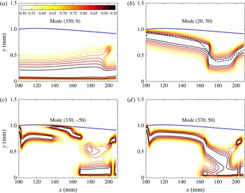
Amplitudes of the streamwise velocity disturbances normalized by the local wall-normal maximums for four modes. The contour levels range from 0.5 to 0.95 with steps of 0.05. The dashed-dotted line denotes the position of the boundary layer edge. (a) Mode
 $(350,0)$
; (b) mode
 $(20,50)$
with the dashed line denoting the critical layer location; (c) mode
 $(330,-50)$
; (d) mode
 $(370,50)$
.

The amplitudes in figure 15 only show the maximum temperature perturbations. To better visualize the evolution of the disturbances, the contours of the streamwise velocity perturbations for
 $(350,0)$
,
 $(20,50)$
,
 $(330,-50)$
and
 $(370,50)$
are plotted in figure 19. The main part of the second mode initially lies below
 $y=0.5$
mm (close to the sonic line) and then slowly expands upwards for
 $x>160$
mm where the nonlinear effects set in. The peak amplitude of the Görtler mode, however, is slightly below the critical layer (denoted by the dashed line). The critical layer is the position where the local laminar mean velocity is equal to the phase velocity. The excellent match between the peak locations and the critical layer locations strongly suggests that the Görtler mode moves with the local mean-flow velocity, a prominent feature of a vortex. The maximum location moves slowly downwards before
 $x=170$
mm, which is consistent with the decrease in the boundary layer thickness, and then sharply drops from
 $y\approx 0.8$
mm at
 $x=170$
mm to
 $y\approx 0.4$
mm at
 $x=180$
mm. This sudden shape change may be caused by the nonlinear forcing by the second mode and the difference/sum modes as will be illustrated below. The difference mode
 $(330,-50)$
mainly lies on the critical layer and the boundary layer edge until
 $x=160$
mm where these two humps merge and a new peak appears close to the wall. For
 $x>180$
mm, the hump near the critical layer has totally disappeared, while the hump near the wall has spread out to cover the lower half of the boundary layer. The shape evolution of sum mode
 $(370,50)$
is similar to that of the difference mode with the only difference being that only one hump exists in the linear stage. The downwards shift of the difference-/sum-mode shapes may result from a combination of a nonlinear force mainly from the second mode and the linear characteristics of the modes themselves, since they lie close to the second-mode parameter region (see figure 6) and, thus, probably tend to behave like the second mode. Indeed, in a simulation (not shown here) with the nonlinear forces turned off once the difference/sum modes were generated showed that their shapes quickly moved downwards within a distance less than 2 mm to cover the lower half of the boundary layer. The difference-/sum-mode shape changes eventually lead to the sudden change of the Görtler mode distribution in the synchronization stage where the nonlinear forces manifest themselves.
5.3.1 Kinetic energy budget
The PSE results described above involve the rapid growth of the Görtler mode and the rapid decay of the second mode. However, it is not obvious whether the second mode acts only as a catalyst, allowing the mean flow to transfer energy to the Görtler mode, or if the second mode directly supplies energy to the low-frequency components. The kinetic energy equation for each mode is used to answer this question. Similar energy analyses of incompressible flows were given by Orszag & Patera (Reference Orszag and Patera1983) in their study of secondary instability in wall-bounded shear flows and by Hajj, Miksad & Powers (Reference Hajj, Miksad and Powers1993) in their study of the fundamental subharmonic resonance in a free shear flow. The streamwise moment equation of the NPSE equations (3.4) for one mode, say
 $(m,n)$
, can be rewritten as
 $$\begin{eqnarray}\bar{\unicode[STIX]{x1D70C}}\frac{\text{D}u}{\text{D}t}=-{\mathcal{L}}_{u}\unicode[STIX]{x1D6F9}+{\mathcal{N}}_{u},\end{eqnarray}$$
where
 ${\mathcal{L}}_{u}$
denotes the linear operator and
 ${\mathcal{N}}_{u}$
denotes the nonlinear terms. The subscript
 $(m,n)$
has been omitted for simplicity. The density variations have been moved to the right-hand side and the non-parallel components have been absorbed into
 ${\mathcal{L}}_{u}$
. The density variations in the moment perturbation equations (5.12) only appear in the non-parallel terms and the nonlinear perturbation terms.
Multiply equation (5.12) by
 $u^{\ast }$
(the complex conjugate of
 $u$
), multiply the complex conjugate of equation (5.12) by
 $u$
, and then add these two equations to get:
 $$\begin{eqnarray}\bar{\unicode[STIX]{x1D70C}}\frac{\text{D}|u|^{2}}{\text{D}t}\equiv -2\unicode[STIX]{x1D6FC}_{i}\bar{U}\bar{\unicode[STIX]{x1D70C}}|\hat{u} |^{2}\exp \left(-2\int \unicode[STIX]{x1D6FC}_{i}\,\text{d}x\right)=-u^{\ast }{\mathcal{L}}_{u}\unicode[STIX]{x1D6F9}+u^{\ast }{\mathcal{N}}_{u}+\text{c.c.},\end{eqnarray}$$
where the PSE assumption (3.1) has been applied. Similar operations to the spanwise and wall-normal moment equations give the kinetic energy equation for one mode as
 $$\begin{eqnarray}\frac{1}{2}\bar{\unicode[STIX]{x1D70C}}\frac{\text{D}}{\text{D}t}(|u^{2}|+|v^{2}|+|w^{2}|)\equiv -\unicode[STIX]{x1D6FC}_{i}\bar{U}\bar{\unicode[STIX]{x1D70C}}(|\hat{u} |^{2}+|\hat{v}|^{2}+|{\hat{w}}|^{2})\exp \left(-2\int \unicode[STIX]{x1D6FC}_{i}\,\text{d}x\right)={\mathcal{L}}+{\mathcal{N}},\end{eqnarray}$$
where
 $$\begin{eqnarray}{\mathcal{L}}\equiv {\textstyle \frac{1}{2}}(-u^{\ast }{\mathcal{L}}_{u}\unicode[STIX]{x1D6F9}-v^{\ast }{\mathcal{L}}_{v}\unicode[STIX]{x1D6F9}-w^{\ast }{\mathcal{L}}_{w}\unicode[STIX]{x1D6F9}+\text{c.c.}),\end{eqnarray}$$
and
 $$\begin{eqnarray}{\mathcal{N}}\equiv {\textstyle \frac{1}{2}}(u^{\ast }{\mathcal{N}}_{u}+v^{\ast }{\mathcal{N}}_{v}+w^{\ast }{\mathcal{N}}_{w}+\text{c.c.}).\end{eqnarray}$$
Here we have defined the reduced kinetic energy per unit volume as
 $$\begin{eqnarray}e\equiv {\textstyle \frac{1}{2}}\bar{\unicode[STIX]{x1D70C}}(|u|^{2}+|v|^{2}+|w|^{2}),\end{eqnarray}$$
which is consistent with the integrand of the norm used in the PSE (see (3.8)).
 ${\mathcal{L}}$
includes the energy exchanged per unit volume between the mode itself and the undisturbed mean flow, as well as dilatation/viscous dissipation.
 ${\mathcal{L}}$
is apparently caused by linear mechanisms although nonlinear forces exert an indirect influence on the energy exchange through changing the mode shapes or the disturbances amplitudes.
 ${\mathcal{N}}$
represents the energy variation caused by nonlinear mechanisms. Unlike the incompressible case where
 ${\mathcal{N}}$
only consists of disturbance variables and can be interpreted as the energy exchange between disturbance modes,
 ${\mathcal{N}}$
here contains the mean-flow variables which indicates that modes can absorb/lose energy from/to the mean flow as well as other modes.
The linear energy transfer can be further divided into five parts as
 $$\begin{eqnarray}{\mathcal{L}}={\mathcal{P}}+\unicode[STIX]{x1D6EF}+{\mathcal{C}}+\unicode[STIX]{x1D6F1}+{\mathcal{V}},\end{eqnarray}$$
where
 $$\begin{eqnarray}\displaystyle {\mathcal{P}}=-\bar{\unicode[STIX]{x1D70C}}u^{\ast }v\frac{\unicode[STIX]{x2202}\bar{U}}{\unicode[STIX]{x2202}y}+\text{c.c.}, & & \displaystyle\end{eqnarray}$$
 $$\begin{eqnarray}\displaystyle \unicode[STIX]{x1D6EF} & = & \displaystyle -\bar{\unicode[STIX]{x1D70C}}u^{\ast }u\frac{\unicode[STIX]{x2202}\bar{U}}{\unicode[STIX]{x2202}x}-\left(u^{\ast }\frac{\unicode[STIX]{x2202}u}{\unicode[STIX]{x2202}y}+v^{\ast }\frac{\unicode[STIX]{x2202}v}{\unicode[STIX]{x2202}y}+w^{\ast }\frac{\unicode[STIX]{x2202}w}{\unicode[STIX]{x2202}y}\right)\bar{\unicode[STIX]{x1D70C}}\bar{V}-\bar{\unicode[STIX]{x1D70C}}v^{\ast }u\frac{\unicode[STIX]{x2202}\bar{V}}{\unicode[STIX]{x2202}x}-\bar{\unicode[STIX]{x1D70C}}v^{\ast }v\frac{\unicode[STIX]{x2202}\bar{V}}{\unicode[STIX]{x2202}y}\nonumber\\ \displaystyle & & \displaystyle -\,u^{\ast }\unicode[STIX]{x1D70C}\left(\bar{U}\frac{\unicode[STIX]{x2202}\bar{U}}{\unicode[STIX]{x2202}x}+\bar{V}\frac{\unicode[STIX]{x2202}\bar{U}}{\unicode[STIX]{x2202}y}\right)-v^{\ast }\unicode[STIX]{x1D70C}\left(\bar{U}\frac{\unicode[STIX]{x2202}\bar{V}}{\unicode[STIX]{x2202}x}+\bar{V}\frac{\unicode[STIX]{x2202}\bar{V}}{\unicode[STIX]{x2202}y}\right)+\text{c.c.},\end{eqnarray}$$
 $$\begin{eqnarray}\displaystyle {\mathcal{C}}=-\unicode[STIX]{x1D705}\bar{\unicode[STIX]{x1D70C}}u^{\ast }v\bar{U}-\bar{\unicode[STIX]{x1D70C}}w^{\ast }w(\bar{U}g+\bar{V}h)+\unicode[STIX]{x1D705}\bar{\unicode[STIX]{x1D70C}}\bar{V}u^{\ast }u-\unicode[STIX]{x1D705}\bar{U}^{2}\unicode[STIX]{x1D70C}v^{\ast }+\text{c.c.}, & & \displaystyle\end{eqnarray}$$
with
 $$\begin{eqnarray}\displaystyle g\equiv \frac{\sin \unicode[STIX]{x1D703}}{r}\quad \text{and}\quad h\equiv \frac{\cos \unicode[STIX]{x1D703}}{r}, & & \displaystyle\end{eqnarray}$$
 $$\begin{eqnarray}\displaystyle \unicode[STIX]{x1D6F1}=-u^{\ast }\frac{\unicode[STIX]{x2202}p}{\unicode[STIX]{x2202}x}-v^{\ast }\frac{\unicode[STIX]{x2202}p}{\unicode[STIX]{x2202}y}-w^{\ast }\frac{\unicode[STIX]{x2202}p}{\unicode[STIX]{x2202}z}+\text{c.c.} & & \displaystyle\end{eqnarray}$$
Here,
 ${\mathcal{P}}$
is the production,
 $\unicode[STIX]{x1D6EF}$
is the energy transfer associated with the non-parallel terms,
 ${\mathcal{C}}$
is the energy transfer due to the curvature effects,
 $\unicode[STIX]{x1D6F1}$
is the pressure diffusion and dilatation.
 $g$
and
 $h$
denote the transverse curvature and the divergence of the geometry. The viscous dissipation and diffusion term,
 ${\mathcal{V}}$
, is lengthy and is not shown here.
Contours of the normalized energy transfers for mode
 $(20,50)$
. The energy transfers are normalized by the maximum value at each streamwise location. The dashed lines denote negative values while the solid lines denote positive values. The contours range from
 $-0.9$
to 0.9 with steps of 0.2. The boundary layer edge and critical layer are also indicated by thick black lines. (a) Linear energy transfer,
 ${\mathcal{L}}$
. (b) Nonlinear energy transfer,
 ${\mathcal{N}}$
.

Figure 20 illustrates the distributions of the normalized linear and nonlinear energy transfers in the
 $x$
–
 $y$
plane for the Görtler mode. The linear energy transfer is concentrated in the critical layer and is mostly positive. In contrast, the nonlinear energy transfer is concentrated near the boundary layer edge during the linear stage and then gradually covers the entire boundary layer. The broadening of this distribution may be related to the separation of the critical layers of the modes as shown in figure 16(b). Moreover, the boundary layer edge during the linear stage appears to be a separation line between the positive and negative nonlinear transfers with the positive transfers below the line and the negative transfers above the line. During the parametric-resonance stage, however, the positive nonlinear energy transfers are mainly above the critical layer while the negative nonlinear energy transfers are mainly below the critical layer.
Equation (5.14) can be integrated with respect to the wall-normal coordinate,
 $y$
, and divided by
 $$\begin{eqnarray}\unicode[STIX]{x1D6E4}\equiv \int _{0}^{\infty }\bar{\unicode[STIX]{x1D70C}}(|\hat{u} |^{2}+|\hat{v}|^{2}+|{\hat{w}}|^{2})\exp \left(-2\int \unicode[STIX]{x1D6FC}_{i}\,\text{d}x\right)\bar{U}\,\text{d}y,\end{eqnarray}$$
to give
 $$\begin{eqnarray}-\unicode[STIX]{x1D6FC}_{i}={\mathcal{L}}_{\unicode[STIX]{x1D6E4}}+{\mathcal{N}}_{\unicode[STIX]{x1D6E4}},\end{eqnarray}$$
where
 $$\begin{eqnarray}{\mathcal{L}}_{\unicode[STIX]{x1D6E4}}\equiv \int _{0}^{\infty }{\mathcal{L}}\,\text{d}y/\unicode[STIX]{x1D6E4},\quad {\mathcal{N}}_{\unicode[STIX]{x1D6E4}}\equiv \int _{0}^{\infty }{\mathcal{N}}\,\text{d}y/\unicode[STIX]{x1D6E4}.\end{eqnarray}$$
 ${\mathcal{L}}_{\unicode[STIX]{x1D6E4}}$
represents the growth rates due to linear terms while
 ${\mathcal{N}}_{\unicode[STIX]{x1D6E4}}$
represents the growth rates due to nonlinear terms. The subscript
 $\unicode[STIX]{x1D6E4}$
denotes an integral as defined in (5.26).
Linear and nonlinear energy transfers for (a) the second mode
 $(350,0)$
with the dashed lines representing the self-interaction case and dashed-dotted line representing the linear case; (b) the Görtler mode
 $(20,50)$
with the dashed line denoting the linear case; (c) the difference mode (solid lines) and the sum mode (dashed lines).

The streamwise development of the integrated linear and nonlinear energy transfers of the second mode, the Görtler mode and the difference/sum modes are plotted in figure 21. For the second mode, the self-interactions remarkably reduce the linear energy transfer, which is the reason why the second mode saturates. When the back reaction of the Görtler mode arises at
 $x>190$
mm, the energy gain by the linear energy transfer and the energy loss by the nonlinear energy transfer both increase sharply. The nonlinear energy loss is larger than the linear energy gain, so the second mode decreases. For the Görtler mode during the parametric-resonance stage, the linear energy transfer increases sharply to be four times that of the linear case. During this stage, the nonlinear energy transfer is, however, negative but its amplitude is only one-fourth that of the linear energy transfer. Thus, the rapid growth of the Görtler mode follows from the sharp increase in the linear energy transfer rather than direct promotion from the second mode. In contrast, for the difference/sum modes, the linear energy transfers are mostly negative while the nonlinear energy transfers are mostly positive. Their amplitudes are comparable and evolve in a similar manner. The nonlinear energy transfers are slightly larger than the linear energy transfers which then causes the difference/sum modes to grow.
Linear energy budget for mode (20,50). The dashed lines correspond to the linear case.

Figure 22 shows the linear energy budget for mode
 $(20,50)$
. The integrated production term,
 ${\mathcal{P}}_{\unicode[STIX]{x1D6E4}}$
, dominates while the other four parts play secondary roles. In particular,
 ${\mathcal{P}}_{\unicode[STIX]{x1D6E4}(20,50)}$
increases to be six times larger from
 $160$
mm to
 $180$
mm. This observation with the results on the nonlinear energy transfers mentioned earlier lead to the conclusion that the second mode, instead of directly providing energy, mediates the energy transfer from the mean flow to the Görtler mode by significantly strengthening the energy production. The sharp growth of the production term is also seen for other cases in regions
 $B$
and
 $D$
in figure 9(c) and is, therefore, a general mechanism accounting for the rapid growth of the low-frequency mode.
5.4 Interaction between a second-mode wave and a pair of first-mode waves
The parametric study in § 5.1 shows that interactions between a second-mode wave and a single first-mode wave can hardly lead to transition in the present investigation. However, we will demonstrate in this subsection that interactions between a second-mode wave and a pair of oblique first-mode waves (case II) can also effectively induce transition. Please note that all the interactions observed in case I can all be found in case II. In this case, a second-mode wave
 $(350,0)$
and a pair of oblique first-mode waves
 $(60,\pm 30)$
were initially added at
 $x=100$
mm. The initial amplitudes are the same as those in case I. Mode
 $(60,30)$
was chosen because it is the most amplified first mode in the linear case. In addition to the fifteen modes in case I, three more modes were also included for the
 $(0,60)$
,
 $(0,120)$
spanwise MFDs and the
 $(350,60)$
fundamental oblique wave. Mode
 $(0,60)$
is generated by the pair of oblique first-mode waves and interacts with itself to give birth to
 $(0,120)$
and with the second mode to generate
 $(350,60)$
. In case II, each single oblique mode should be understood to be paired with its counterpart unless otherwise stated. For example, the
 $(60,30)$
mode is in fact the
 $(60,\pm 30)$
modes.
Maximum r.m.s of the temperature disturbance for case II (a). Eight selected modes and other higher-order modes (denoted by the grey lines). (b) Time- and azimuthal-averaged skin friction coefficient.

The downstream development of the amplitudes of these eighteen modes are shown in figure 23(a). Similar to case I, these curves were obtained from the wall-normal maximums of the r.m.s. of the temperature disturbances. The amplitudes of
 $(0,60)$
and
 $(350,60)$
grow rapidly and lead to breakdown of the PSE simulation at approximately
 $x=200$
mm. This observation indicates that the dominating interaction mechanism is the fundamental resonance among the second mode,
 $(0,60)$
and
 $(350,60)$
, rather than the combination resonance among the detuned modes as in case I. The skin friction plotted in figure 23(b) closely resembles that in case I, shown in figure 15(c), indicating that both cases undergo similar transition processes.
Numerical settings for all four simulations.

To further explore the driving mechanism, three simplified simulations were conducted with the different settings shown in table 1. The first simulation (
 $S1$
) consists of only the second mode, its first harmonic, the MFD, the pair of first-mode waves,
 $(0,60)$
and
 $(350,60)$
. The second simulation (
 $S2$
) is the same as
 $S1$
except that the streamwise curvature is set to zero. In this simulation, the first mode at the inlet is slightly stable and its initial amplitude was set to
 $10^{-2}$
instead of
 $10^{-3}$
to achieve nearly the same breakdown positions as in the full model. The third simulation (
 $S3$
) includes the second mode, its first harmonic, the MFD,
 $(0,60)$
and
 $(350,60)$
. The initial amplitude of
 $(0,60)$
was set to
 $10^{-5}$
so that the breakdown position was close to those in the other simulations.
Maximum of r.m.s. of temperature disturbance versus downstream distance for the case II: comparison of several selected modes for the full model and the other three simulations.

Normalized streamwise velocity disturbances of the
 $(0,60)$
mode for the full model (solid lines) and simulation
 $S3$
(dashed lines) at three streamwise positions: (a)
 $x=140$
mm, (b)
 $x=170$
mm and (c)
 $x=188$
mm. The Floquet theory results (dotted lines) are displayed in (b) and (c) for comparison.

The results of these three simulations are displayed in figure 24 with comparison to the full model. The evolutions of these three simulations and the full model all enter the parametric-resonance stage at approximately
 $x=170$
mm after which the amplitudes of the spanwise MFD and the fundamental oblique mode are all amplified at nearly the same rates. This confirms the dominant role played by the fundamental resonance. Figure 25 further shows that the mode shapes eventually collapse to the one predicted by Floquet theory, despite the large differences during the linear stage. Similar trends were observed for other primary disturbances (not shown here). Therefore, this fundamental resonance appears to be an ‘attractor’, that is, once the spanwise MFD is present regardless of whether it was initially seeded (as in
 $S3$
) or was nonlinearly generated (as in
 $S1$
,
 $S2$
and the full model), resonance will occur downstream, and the growth rates and mode shapes will be independent of the linear stage. In addition, the
 $S2$
result shows that this type of resonance is also insensitive to the streamwise curvature and, thereby, will be found in boundary layers over straight cones.
The PSD (a) and bicoherence spectra (b) at
 $x=180$
mm. The dashed line represents the
 $N$
factors from the LST results. The bicoherence contour level step is 0.02.

Finally, it should be noted that for the pair of low-frequency modes in region
 $B$
in figure 9(c), the combination resonance is also strong and the dominant interaction may be either the fundamental resonance or the combination resonance depending on their growth rates.
6 Comparison with experiments
The detailed experimental settings were documented in Zhang et al. (Reference Zhang, Tang and Lee2013, Reference Zhang, Zhu, Chen, Yuan, Wu, Chen, Lee and Gad-el-Hak2015) and Zhu et al. (Reference Zhu, Zhang, Chen, Yuan, Wu, Chen, Lee and el Hak2016). The data set consists of PCB data taken in the PKU experiments. The cutoff frequency of the PCB sensors was 11 kHz; hence, data points with frequencies below 11 kHz are not accurate. Figure 26(a) shows the power spectrum densities (PSD) of the time series at
 $x=180$
mm. The dashed line displays the
 $N$
-factors of the amplified frequencies at this location. A prominent hump over the frequency range, 300–400 kHz, is identified to be a second-mode wavepacket since it has the same frequency range as the second mode predicted by LST. The harmonic wavepacket over the frequency range, 600–800 kHz, is also visible. The bicoherence spectrum (see the detail in appendix A) shown in figure 26(b) further indicates three possible interactions. The strong peak at (
 $f_{2nd},f_{2nd}$
) represents the self-interaction of the second-mode wave. The peak centred on
 $(f_{2nd},f_{low})$
denotes the interactions between the second-mode wave and the low-frequency waves while the peak centred on
 $(2f_{2nd},f_{low})$
represents the interactions between the harmonic and the low-frequency waves. The intensities of the nonlinear effects change over the height of the boundary layer (Bountin, Shiplyuk & Maslov Reference Bountin, Shiplyuk and Maslov2008). Very close to the wall, the intensity decreases, resulting in very small bicoherence in the surface pressure measurements. Therefore, as Munoz et al. (Reference Munoz, Heitmann and Radespiel2014) pointed out, analyses such as presented in this work can only give an indication on which waves interact and do not necessarily indicate the intensity of the nonlinear effects.
Comparison of the measured PCB data and the PSE predictions for the wall-pressure amplitudes. (a) The second-mode wave amplitude. The PCB data were derived from the r.m.s. of the filtered time series with the passband (330 kHz, 370 kHz). The PSE results are for the same conditions as the simulation in § 5.3. The initial PSE value was set equal to the PCB data at this point for comparison. (b) The low-frequency wave amplitudes. PCB data were derived from the r.m.s. of the filtered time series with the passband (11 kHz, 70 kHz). The PSE results are the grey lines which represent 63 cases in the parametric study (see § 5.1) with frequencies ranging from 10 to 70 kHz and azimuthal wavenumbers ranging from 10 to 90. The numerical values of the PSE results in (b) were multiplied by
 $10^{4}$
for comparison.

Figure 27 compares the r.m.s. of the wall-pressure disturbances from the PCB data and the PSE results for the second-mode components and the low-frequency components. The PCB data agree qualitatively with the PSE results (taken from § 5.3) for the second-mode components. The peak in the experimental curve is smaller than that in the PSE curve, which is possibly due to two factors. First, the initial second-mode amplitude in the experiments may be slightly smaller. Second, the ‘spatial averaging’ effect of the PCB sensors due to their finite length (approximately one-third of the second-mode wavelength) of the sensor area tends to reduce the measured amplitudes, as was also observed by Berridge et al. (Reference Berridge, Chou, Ward, Steen, Gilbert, Juliano, Schneider and Gronvall2010).
The situation for the low-frequency components, however, is much more complex. Since the wind tunnel was operated under noisy conditions, the major part of the low-frequency components likely consist of acoustic disturbances emitted from the turbulent boundary layer on the wind tunnel wall or vortical disturbances in the free stream. Moreover, the wall-pressure fluctuations of the low-frequency oblique waves are quite small as shown in figure 8, which results in a low signal-to-noise ratio. Therefore, the results in figure 27(b) show that the low-frequency components detected in the experiments grow at a moderate rate along the entire length, with the large difference with the most amplified mode predicted by PSE. And the growth of the low-frequency components seen in the experiments may be either the reflection of the growth of the ambient tunnel noise, as suggested by Kimmel & Kendall (Reference Kimmel and Kendall1991) and Lachwicz et al. (Reference Lachwicz, Chokani and Wikinson1996), or resonance with the second-mode waves, as investigated in the present article, or both. These ambiguities can be clarified with quiet wind tunnel experiments with controlled disturbances combined with more detailed measurements (such as hot-wire or particle image velocimetry (PIV) measurements).
7 Summary and discussion
The stability of a hypersonic boundary layer on a flared cone was analysed for the same flow conditions as in previously conducted experiments (Zhang et al. Reference Zhang, Tang and Lee2013, Reference Zhang, Zhu, Chen, Yuan, Wu, Chen, Lee and Gad-el-Hak2015; Zhu et al. Reference Zhu, Zhang, Chen, Yuan, Wu, Chen, Lee and el Hak2016). LST results show three instabilities in the flared region, i.e. the first mode, the second mode and the Görtler mode. The two-dimensional second mode is most unstable with a dominant frequency of approximately 350 kHz. The first mode covers a large frequency band from 10 to 250 kHz. The dominant mode has a frequency of approximately 60 kHz with an azimuthal wavenumber of 30. The Görtler mode also occupies a large frequency band from 0 to 230 kHz with a dominant azimuthal wavenumber of 90.
The interactions between the second mode and the low-frequency modes, which are indicated by the bicoherence measurements in the experiments, were investigated by solving the NPSE. The parametric study shows that very low-frequency modes (belonging to the unsteady Görtler vortices with frequencies below about 30 kHz and azimuthal wavenumbers around 50) are most heavily promoted. The typical evolution of the low-frequency mode is divided into the linear stage, the synchronization stage, the parametric-resonance stage and the full-interaction stage. During the linear stage, although the low-frequency mode evolves linearly, it interacts with the second mode to drive a fast growing difference mode as well as a sum mode. When the amplitudes of these nonlinearly forced modes become close to that of the low-frequency mode, the low-frequency mode may become saturated or slightly attenuated due to the reactions of the difference/sum modes. Meanwhile, the wavenumbers of the low-frequency and difference/sum modes are rapidly adjusted so that these modes become synchronized with the second mode in the sense that the resonance condition is approximately satisfied. As a result, the low-frequency mode enters into the parametric-resonance stage where it grows much faster than linear theory predicts. Because of the rapid growth, the low-frequency mode soon becomes strong enough to produce a feedback effect on the second mode (the full-interaction stage), which rapidly weakens the second mode. During the linear stage, the phase velocities of the disturbances are nearly the same and phase-locked theory can be applied. However, the phase velocity of the low-frequency mode decreases sharply during the synchronization stage due to the rapid wavenumber changes. Consequently, the phase velocities of the low-frequency mode and the second mode become quite different during the parametric-resonance stage so phase-locked theory may not be suitable. Nevertheless, the parametric-resonance can be well described by Floquet theory and the interaction is seen to be a combination or a fundamental resonance of the secondary instability. The energy method analysis further shows that the rapid growth of the low-frequency mode is solely due to the sharp increase of the Reynolds stress work which is a ‘linear’ mechanism. In contrast, the rapid growth of the difference/sum modes and the rapid decay of the second mode are solely due to the work done by the nonlinear terms.
The parametric study also shows that the interactions between a second-mode wave and a single first-mode wave are weak. However, a pair of first-mode waves will generate a spanwise MFD which will then interact with the second mode to drive a fundamental oblique wave. Instead of the combination resonance, a fundamental resonance occurs downstream between the second mode, the spanwise MFD and the fundamental oblique wave which makes the latter two grow rapidly. For a pair of very low-frequency oblique waves, the combination resonance can also be strong, and can coexist with the fundamental resonance.
The evolutions of the second-mode waves are in qualitative agreements with the results of the PKU experiments. However, there is still ambiguity about the evolution of the low-frequency components, and more detailed measurements using controlled experiments in the quiet wind tunnel are required.
One interesting finding in the present study is the attractor-like character of the parametric resonance in the transitional boundary layer, in the sense that modes with certain frequencies and azimuthal wavenumbers will always come into resonance once the amplitudes of the difference/sum modes are comparable to that of the low-frequency mode (which means that the trajectory is close to the resonance orbit). The parametric resonance seems to depend only on the saturated state of the second mode and, hence, is likely active in other second-mode dominated boundary layers (like the boundary layers over straight cones studied by Sivasubramanian & Fasel (Reference Sivasubramanian and Fasel2014, Reference Sivasubramanian and Fasel2015)). For those boundary layers, however, the low-frequency waves may have no counterparts of the linear instabilities and more likely arise from either the sideband interactions of the unstable waves or interactions between a pair of oblique unstable waves. The latter possibility was confirmed at least for the first mode in § 5.4, while the former possibility was shown to be likely in an unpublished study of interactions between a planar second-mode wave and an oblique second-mode wave (results not shown here).
Acknowledgements
The authors are grateful to Professor X. Wu at Imperial College London and Professor J. Luo at Tianjin University for useful discussions. The work was supported by the National Natural Science Foundation of China (grant nos. 109103010062, 10921202, 11372009, 11602005 and 11632002) and Foundation for Innovative Research Groups of the National Natural Science Foundation of China (grant no. 11521091).
Appendix A. Bicoherence
The bispectrum is defined as
 $$\begin{eqnarray}B(f_{1},f_{2})=E[X(f_{1})X(f_{2})X^{\ast }(f_{1}+f_{2})],\end{eqnarray}$$
where
 $E[\cdot ]$
is the expected value,
 $X(f)$
is the Fourier transform of a segment of the time series record and the superscript asterisk denotes the complex conjugate. Since the value of the bispectrum depends on the magnitude as well as the phase of the components, the bispectrum is usually normalized to obtain the bicoherence,
 $$\begin{eqnarray}b^{2}(f_{1},f_{2})=\frac{|B(f_{1},f_{2})|^{2}}{E[|X(f_{1})X(f_{2})|^{2}]E[|X(f_{1}+f_{2})|^{2}]},\end{eqnarray}$$
which is bounded by zero and one. The bicoherence provides a measure of the degree of the quadratic interaction exhibited by the given triad of waves at frequencies
 $f_{1}$
,
 $f_{2}$
and
 $f_{3}$
that satisfy the resonance wave matching requirement
 $f_{3}=f_{1}+\,f_{2}$
(Shiplyuk et al.
Reference Shiplyuk, Bountin, Maslov and Chokani2003). For totally independent waves, the bicoherence will vanish, while for coupled waves the statistical averaging in (A 2) will yield a non-zero value of the bispectrum. The bicoherence is symmetric in the
 $f_{1}$
,
 $f_{2}$
plane about the three lines
 $f_{1}=f_{2}$
,
 $f_{2}=0$
and
 $f_{1}+f_{2}=f_{N}$
(the Nyquist frequency) because of the relation
 $X(-f)=X^{\ast }(f)$
between the Fourier components. Thus, difference-mode interactions of the form
 $f_{3}-f_{1}=f_{2}$
and
 $f_{3}-f_{2}=f_{1}$
appear at the same point as the sum-mode interactions,
 $f_{3}=f_{1}+\,f_{2}$
. Due to the symmetry properties, the bicoherence can be simply computed over the triangular region
 $$\begin{eqnarray}0\leqslant f_{1}\leqslant f_{N};\quad 0\leqslant f_{2}\leqslant 1/2f_{N}.\end{eqnarray}$$
Appendix B. Code validation
Dimensional temperature and streamwise velocity distributions in the wall-normal direction at
 $x=330$
mm for the Langley 93–10 flared cone. The symbols are taken from Pruett & Chang (Reference Pruett and Chang1998).

Test cases for LST code.

Growth rates of the subharmonic resonance predicted by Floquet theory for three different amplitudes of the primary wave (the second mode) for a Mach 4.5 flat-plate boundary layer.
 $\unicode[STIX]{x1D6FD}$
is the spanwise wavenumber of the secondary wave. The reference length is the displacement thickness. The symbols are taken from the results of Ng & Erlebacher (Reference Ng and Erlebacher1992).

Subharmonic and fundamental resonances for a Mach 1.6 flat-plate boundary layer. The symbols are taken from the PSE results of Chang & Malik (Reference Chang and Malik1994).

The code validation consisted of four parts for the mean-flow code, LST code, Floquet analysis code and NPSE code. The first part used the mean-flow calculations of the boundary layer over the Langley 93–10 flared cone with excellent agreement with the results of Pruett & Chang (Reference Pruett and Chang1998), as shown in figure 28. The second part examined the accuracy of the LST code by comparing four test cases with the results of Malik (Reference Malik1990) in table 2, again with good agreement. The third part calculated a subharmonic instability for different amplitudes of the primary wave for a Mach 4.5 boundary layer with the Floquet analysis code with very good agreement with the results of Ng & Erlebacher (Reference Ng and Erlebacher1992) in figure 29. Finally, the subharmonic/fundamental resonances in a Mach 1.6 flat-plate boundary layer were calculated with the NPSE code with good agreement with the results of Chang & Malik (Reference Chang and Malik1994) as shown in figure 30.