


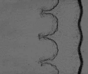

1. Introduction
When an impulsive acceleration, such as a shock wave, is exerted on a perturbed fluid interface with distinct densities, Richtmyer–Meshkov (RM) instability is triggered (Richtmyer Reference Richtmyer1960; Meshkov Reference Meshkov1969). Conversely, when continuous accelerations caused by such as rarefaction waves are exerted, Rayleigh–Taylor (RT) instability or stabilization occurs (Rayleigh Reference Rayleigh1883; Taylor Reference Taylor1950; Mikaelian Reference Mikaelian2009), depending upon whether the rarefaction waves propagate from heavy fluids into light fluids or vice versa. Interfacial instabilities have received much attention due to their significant role in various scientific and engineering applications such as supernova explosions (Kuranz et al. Reference Kuranz, Park, Huntington, Miles, Remington, Plewa, Trantham, Robey, Shvarts and Shimony2018; Musci et al. Reference Musci, Petter, Pathikonda, Ochs and Ranjan2020), supersonic combustions (Yang, Chang & Bao Reference Yang, Chang and Bao2014) and inertial confinement fusion (ICF) (Betti & Hurricane Reference Betti and Hurricane2016; Chu et al. Reference Chu, Wang, Qi, Xu and Li2022). In these applications, shocks and rarefaction waves, which provide complex acceleration histories, interact with the interfaces, significantly influencing the development of flow structures. Specifically, in ICF implosions, the shock wave arrives at the light layers, generating reflected rarefaction waves that rarefy the previously shocked layers (Lindl et al. Reference Lindl, Landen, Edwards, Moses and Team2014). The shock ultimately reaches the capsule centre and then reflects on itself, reshocking the implosion layers. The interface between the shell materials and fuels mainly experiences the impacts of three waves: the incident shock, the reflected rarefactions from the inner heavy/light interfaces and the reflected shock from the capsule centre (Montgomery et al. Reference Montgomery2018; Peterson, Johnson & Haan Reference Peterson, Johnson and Haan2018). The hydrodynamic instabilities resulting from the interactions between these waves and the shell/fuel interface, cause the mixing of ablator materials and fuels, preventing the fusion yield from reaching positive output (Clark et al. Reference Clark2016). As a result, it is of significance to study the interfacial instabilities induced by successive shocks and rarefactions.
Most previous studies focused on the shock- or reshock-induced RM instability (Brouillette Reference Brouillette2002; Ranjan, Oakley & Bonazza Reference Ranjan, Oakley and Bonazza2011; Zhou Reference Zhou2017a,Reference Zhoub; Zhou et al. Reference Zhou, Clark, Clark, Glendinning, Skinner, Huntington, Hurricane, Dimits and Remington2019, Reference Zhou2021). The shock-induced RM instability has been investigated extensively through theoretical modelling (Goncharov Reference Goncharov2002; Dimonte & Ramaprabhu Reference Dimonte and Ramaprabhu2010; Zhang & Guo Reference Zhang and Guo2016; Liu, Zhang & Xiao Reference Liu, Zhang and Xiao2023), experiments (Jacobs & Krivets Reference Jacobs and Krivets2005; Vanderboomgaerde et al. Reference Vanderboomgaerde, Souffland, Mariani, Biamino, Jourdan and Houas2014; Reese et al. Reference Reese, Ames, Noble, Oakley, Rothamer and Bonazza2018; Mansoor et al. Reference Mansoor, Dalton, Martinez, Desjardins, Charonko and Prestridge2020) and numerical simulations (Holmes et al. Reference Holmes, Dimonte, Fryxell, Gittings, Grove, Schneider, Sharp, Velikovich, Weaver and Zhang1999; Latini, Schilling & Don Reference Latini, Schilling and Don2007; Dell, Stellingwerf & Abarzhi Reference Dell, Stellingwerf and Abarzhi2015; Thornber et al. Reference Thornber, Griffond, Bigdelou, Boureima, Ramaprabhu, Schilling and Williams2019), and the instability evolution in different regimes has been well understood. The impact of reshock on an interface deposits additional vorticity, with the direction being either opposite to or the same as that of vorticity deposited by the shock. In cases with the opposite vorticity direction, initial multi-mode perturbations with reshock were primarily focused on (Balakumar et al. Reference Balakumar, Orlicz, Tomkins and Prestridge2008, Reference Balakumar, Orlicz, Ristorcelli, Balasubramanian, Prestridge and Tomkins2012; McFarland et al. Reference McFarland, Reilly, Black, Greenough and Ranjan2015; Mohaghar et al. Reference Mohaghar, Carter, Musci, Reilly, McFarland and Ranjan2017, Reference Mohaghar, Carter, Pathikonda and Ranjan2019; Sewell et al. Reference Sewell, Ferguson, Krivets and Jacobs2021). In these studies, the reshock impact destroys the shock-induced ordered vorticity field, and thus the transition to turbulence is likely to be achieved. Notably, if the vorticity deposited by the reshock and shock cancels out, the perturbation growth is frozen (Mikaelian Reference Mikaelian1985; Charakhch'yan Reference Charakhch'yan2001; Chen et al. Reference Chen, Xing, Wang, Zhai and Luo2023b). In cases with the same vorticity direction, the shock- and reshock-induced vorticity accumulates, accelerating the instability evolution. Studies on initial single-scale interfaces showed that the reshock impact does not disrupt the existing ordered vorticity field so that the single-scale interface is maintained for a long time after reshock, and the trend of perturbation growth after reshock exhibits similarities to that in singly shocked cases (Guo et al. Reference Guo, Cong, Si and Luo2022a,Reference Guo, Si, Zhai and Luob).
The rarefaction-induced RT instability was first numerically investigated by Li & Book (Reference Li and Book1991) and Li, Kailasanath & Book (Reference Li, Kailasanath and Book1991). It was found that the instability shows rapid growth after the rarefaction impact, resulting in mixing enhancement in supersonic flows. Liang et al. (Reference Liang, Zhai, Luo and Wen2020) studied the RT instability induced by narrow-width rarefactions and considered the effects of interaction periods and the strength of rarefactions on the interface evolution. Wang et al. (Reference Wang, Song, Ma, Ma, Wang and Wang2022b,Reference Wang, Song, Ma, Zhang, Shi, Wang and Wangc) studied the transition behaviour of rarefaction-driven diffuse interfaces and found that the transition is delayed as the interface diffusion intensifies. Theoretically, Mikaelian (Reference Mikaelian2009) developed a generalized Layzer model (GLM) (Layzer Reference Layzer1955) with nonlinear and linear types to describe the rarefaction-induced perturbation growth. It was shown that the linear GLM provides better predictions than the nonlinear GLM in some cases. Additionally, Mikaelian (Reference Mikaelian2009) found that the rarefaction-driven RT instability has a much faster growth rate compared with the shock-induced RM instability. Experimentally, Morgan et al. (Reference Morgan, Cabot, Greenough and Jacobs2018); Morgan, Likhachev & Jacobs (Reference Morgan, Likhachev and Jacobs2016) generated two- (2-D) and three-dimensional (3-D) single-mode interfaces using the membraneless technique (Jones & Jacobs Reference Jones and Jacobs1997), and studied the linear and nonlinear instability evolution in a vertical rarefaction tube. Later, 3-D multi-mode perturbations were generated by Morgan & Jacobs (Reference Morgan and Jacobs2020), and turbulent mixing induced by rarefaction-driven RT instability was focused on.
The interfacial instability driven by successive shocks/rarefactions or rarefactions/shocks is more complex than that caused by a single wave. Previous studies, involving reshock–interface interactions (Hill, Pantano & Pullin Reference Hill, Pantano and Pullin2006; Schilling, Latini & Don Reference Schilling, Latini and Don2007; Lombardini et al. Reference Lombardini, Hill, Pullin and Meiron2011; Li et al. Reference Li, He, Zhang and Tian2019, Reference Li, Tian, He and Zhang2021) and fluid-layer behaviours (Liang & Luo Reference Liang and Luo2021; Cong et al. Reference Cong, Guo, Si and Luo2022), have primarily focused on the interfacial instabilities induced by different waves. In these studies, the constraints imposed by rigid walls or fluid-layer interfaces cause shocks and rarefactions to bounce back and forth, resulting in repeated interactions with the interface. Moreover, compression waves, generated by the impact of rarefactions on a heavy/light interface, interact with the interface, further complicating the flow dynamics. Consequently, in a system where multiple waves continually interact with the interface, isolating the instabilities induced by different waves is challenging.
Mikaelian (Reference Mikaelian2009) numerically studied the interfacial instability induced by two kinds of waves: shock waves and rarefaction waves. The shock and rarefaction waves propagate in opposite directions and interact with the interface only once. According to the sequence of wave arrival at the interface, there were two scenarios. If the rarefactions reach the interface first, the rarefaction-induced RT behaviour remains unchanged although the shock deposits additional vorticity at the interface. Conversely, if the shock reaches the interface first, the interface evolution changes from RM unstable states into RT unstable or stable states, depending on whether the rarefactions impact a heavy/light or light/heavy interface. The second scenario in the work of Mikaelian (Reference Mikaelian2009), i.e. the interaction of counter-directional shock/rarefactions with an interface, actually corresponds to the first part of the interactions of three waves (the incident shock, the co-directional rarefaction and shock waves) with the ablator/fuel interface in the context of ICF, as mentioned at the beginning section. In this scenario, the incident shock effect is significantly attenuated by the impact of rarefaction waves. Particularly, for an initial heavy/light interface, the incident shock effect can, under certain conditions, be completely counteracted by the impact of rarefaction waves (Chen et al. Reference Chen, Wang, Zhai and Luo2023a). Given that the influence of the incident shock would be significantly attenuated, in the interactions of these three waves with an interface, the second part, denoted as the interaction of co-directional rarefactions/shock with an interface, is of great concern. However, the mechanism of instabilities induced by such co-directional waves remains unclear. Particularly, after the shock acceleration, whether the instability maintains the RT evolution state or transforms into RM instability needs to be explored.
In this work, the interfacial instabilities induced by co-directional rarefaction and shock waves are investigated experimentally and theoretically. To facilitate our study, we develop a rarefaction-shock tube that allows for the decoupling of interfacial instabilities caused by these waves. The remainder of this paper is organized into three main sections. The rarefaction-shock tube used in the present work is described in § 2. One-dimensional (1-D) analysis for the flow within this tube is presented in § 3. Experimental and theoretical results of 2-D single-mode interfaces, as well as the analytical theories for describing the rarefaction-induced acceleration and density, are presented in § 4. Finally, conclusions are presented.
2. Experimental apparatus
A rarefaction-shock tube, as sketched in figure 1, is developed to generate co-directional rarefaction and shock waves. The rarefaction-shock tube, with an inner cross-sectional area of  $120\,{\rm mm}\times 6\,{\rm mm}$, has four main sections: a 1.0 metre long vacuum section, a 0.4 metre long transition section, a 0.45 metre long test section and a 1.0 metre long reflection section. The generation process of co-directional rarefaction and shock waves is briefly described as follows. First, a polyethylene terephthalate (PET) diaphragm is used to separate the vacuum and transition sections. Then, air is discharged from the vacuum section using a vacuum pump. When the pressure in the vacuum section reduces to the endurance limit of the PET diaphragm, it is suddenly broken, generating rarefaction waves propagating downstream along the transition section, and a shock propagating upstream along the vacuum section. The shock arrives at the reflection wall in the vacuum section and reflects, returning to chase the rarefactions. As a result, co-directional rarefaction and shock waves are generated.
Schematic of the rarefaction-shock tube.

A complete rupture of the PET diaphragm is necessary for generating high-quality co-directional rarefaction and shock waves. However, it is difficult to achieve complete rupture simply relying on the pressure difference between the vacuum and transition sections, since the cross-section of the tube is too narrow. To solve this problem, a set of diaphragm-breaking clamps, as shown in figure 1, are designed. The clamps contain the left and right two parts, with a sharp, blade-like rectangular edge in the middle of the left part. During the rupture process, due to the pressure difference between the vacuum and transition sections, the diaphragm bulges towards the vacuum section. When the pressure in the vacuum section reduces to the PET diaphragm's endurance limit, the sharp edge of the left part cuts off the whole PET diaphragm, realizing the complete rupture of the diaphragm.
To prevent the interface from running out of the observing window before the shock arrival, it is necessary to control the time of shock reaching the interface. Rectangular plates, which have the same cross-sectional area as the inner cross-section of the tube, are placed as the reflection wall in the vacuum section. By replacing rectangular plates of different lengths, the shock arrival time can be adjusted. The distance from the reflection wall to the diaphragm will be determined by 1-D theory in the next section.
3. One-dimensional rarefaction-shock tube flows
The rarefaction-shock tube flow mainly involves shock reflection, shock–rarefaction interaction, rarefaction–rarefaction interaction, rarefaction–interface interaction and shock–interface interaction. To solve such a complicated flow problem, a detailed 1-D physical analysis of the flow is first presented. Then, theoretical calculations are performed and the  $x$–
 $t$ diagram depicting the motions of waves and interfaces is presented. Finally, experiments of an unperturbed interface impacted by co-directional rarefaction and shock waves are conducted to examine the feasibility of the rarefaction-shock tube.
3.1. Physical analysis
The flow within the rarefaction-shock tube can be categorized into two distinct regions. The first region primarily involves shock reflection and interactions between shocks and contact surfaces, taking place within the vacuum section. The second region mainly involves shock–rarefaction–interface interactions, occurring within the transition and test sections. To ensure a clear understanding of the rarefaction-shock tube flow, the flow features of these two regions will be presented individually.
The distributions of flow regions at specific times primarily observed in the vacuum section are shown in figure 2;  $t = 0$ and
 $x = 0$ are defined as the diaphragm rupture moment and the diaphragm location, respectively. The sudden rupture of the diaphragm generates a left-travelling shock (SW), right-travelling rarefactions (RW) and a contact surface (CS
 $_1$), as depicted in figure 2(b). The SW hits the solid wall and reflects, returning to strike the CS
 $_1$, and consequently, two shocks including a transmitted shock (SW
 ${^t_1}$) and a reflected shock (SW
 $^r_1$) are generated, as depicted in figures 2(c) and 2(d). The SW
 ${^r_1}$ repeats the route of SW, generating a transmitted shock (SW
 ${^t_2}$) and a reflected shock (SW
 ${^r_3}$), as shown in figure 2(e). Theoretically, there are an infinite number of shocks passing through the CS
 $_1$. However, according to 1-D theory (Han & Yin Reference Han and Yin1993; Zucker & Biblarz Reference Zucker and Biblarz2019), which is described in Appendix A, the Mach number of SW
 $_2^t$ in this work is 1.006, and the subsequent transmitted shocks are weaker. Therefore, only the first transmitted shock SW
 ${^t_1}$ is considered. The shock behaviours occurring in the vacuum section are summarized in the
 $x$-
 $t$ diagram, as illustrated in figure 3(a).
Distributions of flow regions at specific times primarily observed in the vacuum section. (a) The initial flow state. (b) The moment just after the diaphragm rupture. (c) The moment before the reflected shock SW $^r$ reaches the contact surface CS
 $_1$. (d) The moment when the SW
 $^r$ has collided with the CS
 $_1$, resulting in the formation of SW
 $_1^r$ and SW
 $_1^t$. (e) The moment when the SW
 $^r_2$ (generated by the SW
 $_1^r$ hitting the solid wall) has collided with the CS
 $_1$, resulting in the formation of SW
 $_3^r$ and SW
 $_2^t$. Here, SW and RW denote the shock and rarefactions generated by the diaphragm rupture, respectively, CS
 $_1$ denotes a contact surface, SW with a superscript ‘
 $r$’ or ‘
 $t$’ denotes reflected or transmitted shocks and similarly hereinafter.

The  $x$–
 $t$ diagrams illustrating the wave dynamics in the vacuum section (a) and in the transition and test sections (b).

The distributions of flow regions at specific times in the transition and test sections are shown in figure 4. Figure 4(a) shows the situation considered in this work: an air/SF $_6$ interface is located in the test section and the rarefactions arrive at the interface before the shock. In figure 4(b), the impact of RW on the interface (CS
 $^I$) generates right-travelling transmitted rarefactions (RW
 $^t$) and left-travelling reflected rarefactions (RW
 $^r_1$). The RW
 $^r_1$ continuously collides with the RW, forming a flow region (RR) which contains both left- and right-travelling waves. In figure 4(c), the SW
 $^t_1$ reaches the tail of RW and then passes through the rarefaction region R, giving rise to left-travelling compression waves (CW) and a contact region (CR
 $_1$). When the SW
 $^t_1$ traverses the rarefaction region R, its intensity gradually diminishes. Here, SW
 $_x$ represents the shock with varying intensity. The SW
 $_x$ transforms the passing rarefaction region (R) into the post-shock flow region, i.e. the position of the SW
 $_x$ becomes the position of the RW tail. Over time, the SW
 $_x$ arrives at the region RR. When passing through the region RR, the SW
 $_x$ interacts not only with the RW but also with the RW
 $^r_1$, resulting in a complex flow pattern. After the collision of SW
 $_x$ with RW
 $^r_1$, a contact region (CR
 $_2$) is formed between the newly generated rarefactions (RW
 $_2^r$) and the shock SW
 $_x$, as shown in figure 4(d).
Distributions of flow regions at specific times in the transition and test sections. (a) The moment when the shock SW $_1^t$ chases the rarefactions RW. (b) The moment when the RW impacts the interface. (c) The moment when the SW
 $_x$ passes through the rarefaction region R. (d) The moment when the SW
 $_x$ passes through the rarefaction region RR. (e) The moment when the SW
 $_x^r$ and SW
 $_x^t$ have left the interface. Here, CW denotes compression waves, RW with a superscript ‘
 $r$’ or ‘
 $t$’ denote reflected or transmitted rarefactions, CR
 $_{1,2}$ denote contact regions. The shock SW
 $_x$ has varying intensity due to continuously traversing the rarefaction region. In (e), the shock SW
 $_x^r$ and SW
 $_x^t$ eliminate the rarefaction regions that they reach, generating a quasi-stable region on both sides of the interface.

The distributions of flow regions after the shock strikes the interface are shown in figure 4(e). There is a quasi-stable region, which emerges due to the transformation of the rarefaction region into the post-shock flow region by the transmitted shock (SW $_x^t$) and the reflected shock (SW
 $_x^r$). Figure 3(b) shows the
 $x$–
 $t$ diagram illustrating the process of the shock–rarefaction–interface interaction that occurs in the transition and test sections. On the left side of the interface, the compression waves (CW), the reflected rarefactions (RW
 $_r^2$) and the reflected shock (SW
 $_x^r$) are all left-travelling waves, which have no impact on the interface evolution. There are two types of perturbations that arrive at the interface following the shock impact. The first type is the right-travelling contact surface, formed due to the shock–rarefaction interaction. The contact surface, with both the pressure and flow velocity being equal on both sides, has a negligible influence on the interface evolution (Han & Yin Reference Han and Yin1993). The second type comprises compression waves generated by SW
 $_x^t$ as it passes through the RW
 $^t$ region, and by SW
 $_x^r$ as it passes through the RW
 $^r_2$ region. Nevertheless, these compression waves reflected from the isentropic rarefaction regions exhibit limited strength (Han & Yin Reference Han and Yin1993), thus having minimal effects on the interface evolution. As a result, the region between SW
 $_x^r$ and SW
 $_x^t$ can be considered quasi-stable.
In short, the physical analysis of 1-D flows demonstrates the feasibility of generating co-directional rarefaction and shock waves by the rarefaction-shock tube. Furthermore, once the shock wave catches up with the rarefaction waves, it effectively eliminates the rarefaction region. Ultimately, a quasi-stable region is formed on both sides of the interface, thereby providing a favourable condition for decoupling the interfacial instabilities induced by rarefaction and shock waves.
3.2. Theoretical calculation
The 1-D theory (see Appendix A) provides a rapid means to determine the motions of waves and interfaces within the tube, thus enabling the assessment of the apparatus's design parameters. In this work, the initial interface location ( $x_0$), which is dependent on the lengths of the transition and test sections, is 710 mm downstream of the diaphragm. This situates the interface roughly one third along the viewing window, ensuring an extensive observation range for interface evolution. The 1-D theoretical result shows that
 $x_0 = 710$ mm allows the rarefaction waves to reach the interface before the shock. Through theoretical calculations and experimental attempts, we place the reflection wall 81 mm upstream of the diaphragm, which ensures that the evolving interface remains a small-perturbation state at the time of shock arrival. Additionally, the reflection section with a one metre length is verified to be sufficiently long. The theoretical result shows that the reflection section causes the reflected wave from the right endwall to reach the evolving interface after
 $t\approx 14$ ms, while our experimental duration is only approximately 5 ms.
Figure 5 shows the  $x$–
 $t$ diagram of the 1-D rarefaction-shock tube flow based on
 $x_0$ of 710 mm and the reflection-wall location
 $x_1$ of
 $-$81 mm. For brevity, the waves on the right side of the interface and on the left side of the shock are not presented. The diaphragm rupture pressure for calculations is 45 kPa, which is consistent with that used in the experiments. Before the shock SW
 $^t_1$ catches up with the rarefaction waves, its Mach number is 1.189. The arrival times of the rarefaction head and the shock at the interface are 2083 and
 $2835\,\mathrm {\mu }$s, respectively. When the shock arrives at the interface, its Mach number decreases to 1.128.
Theoretical  $x$–
 $t$ diagram of the 1-D rarefaction-shock tube flow based on
 $x_0$ of 710 mm and
 $x_1$ of
 $-$81 mm. The initial interface is an unperturbed air/SF
 $_6$ configuration.

3.3. Experimental verification
Experiments of an unperturbed air/SF $_6$ interface accelerated by co-directional rarefaction and shock waves are conducted to examine the feasibility of the rarefaction-shock tube; PET diaphragms with a thickness of
 $3\mathrm {\mu }$m are utilized to separate the vacuum and transition sections, and the diaphragm rupture pressure is
 $45\pm 1$ kPa for each case. The improved soap-film technique is used to generate initial discontinuous interfaces (Li et al. Reference Li, Cao, Wang, Zhai and Luo2023). Acrylic plates, with the borders pre-engraved to be the designed shape (flat for the unperturbed case and sinusoidal for the 2-D single-mode case discussed later) are fabricated into the interface formation device. Then, a super-hydrophobic-oleophobic material is applied to the designated location on the interface formation device to constrain the soap film into the designed shape (Li et al. Reference Li, Cao, Wang, Zhai and Luo2023). The super-hydrophobic-oleophobic coatings have no impact on the flow as they do not introduce obstacles (Wang et al. Reference Wang, Wang, Zhai and Luo2022a). By injecting SF
 $_6$ into the test section to displace air on the right side of the soap-film interface, an air/SF
 $_6$ interface is generated. The volume fraction of air (SF
 $_6$) on the left (right) side of the soap-film interface is nearly 100 % for each case, resulting in an Atwood number
 $(A = (\rho _{h0}-\rho _{l0})/(\rho _{h0}+\rho _{l0})$, with
 $\rho _{l0}$ and
 $\rho _{h0}$ being the densities of light and heavy fluids on both sides of the interface) of 0.67. A high-speed schlieren system, as described in our previous work (Guo et al. Reference Guo, Cong, Si and Luo2022a), is utilized to capture the flow field. Illuminated by a xenon light source, the flow is recorded by a high-speed camera (FASTCAM SA5, Photron Ltd) with a CMOS sensor. The frame rate of the camera is 65 100 frames per second and the exposure time is
 $1\,\mathrm {\mu }$s. The pixel resolution is 0.488 mm pixel
 $^{-1}$. More details about the techniques for the interface formation and flow field measurements can be found in the previous work (Guo et al. Reference Guo, Cong, Si and Luo2022a; Li et al. Reference Li, Cao, Wang, Zhai and Luo2023).
Figure 6(a) shows the schlieren images of the unperturbed air/SF $_6$ interface accelerated by co-directional rarefaction and shock waves. Due to the limitation of schlieren photography, it is very difficult to capture large-width rarefaction waves. Therefore, corresponding schematics are provided below the schlieren images for better comprehension. In figure 6(b), the experimental
 $x$–
 $t$ diagram of the shock and unperturbed interface is presented. Prior to the shock arrival, the interface undergoes variable acceleration motion. At
 $t\approx 2835\,\mathrm {\mu }$s, the shock wave reaches the interface, causing a significant deceleration. Following this, the interface exhibits a tendency of uniform leftward movement. Additionally, figure 6(b) includes the theoretical
 $x$–
 $t$ lines of the shock and interface. The experimental and theoretical results are in good agreement, demonstrating the feasibility of our apparatus in generating co-directional rarefaction and shock waves.
(a) Schlieren images and their corresponding schematics of an unperturbed air/SF $_6$ interface impacted by co-directional rarefaction and shock waves. Numbers denote time with unit of
 $\mathrm {\mu }$s. (b) Comparison of the 1-D motions of the shock and interface between experiments and 1-D theory.

4. Analysis of single-mode interface instabilities
Six kinds of single-mode air/SF $_6$ interfaces with different amplitude–wavelength combinations are considered. The values of initial interface amplitude (
 $a_0$) and wavelength (
 $\lambda$) for different cases are listed in table 1. A number combination such as 1-40 denotes the case with
 $a_0$ of 1 mm and
 $\lambda$ of 40 mm. One can find that the initial amplitude–wavelength ratio (
 $a_0$/
 $\lambda$) for each case is no more than 0.05, satisfying the small-amplitude hypothesis (McFarland, Greenough & Ranjan Reference McFarland, Greenough and Ranjan2014; Liu et al. Reference Liu, Liang, Ding, Liu and Luo2018).
Initial interface parameters for different single-mode cases. Here,  $a_0$ and
 $\lambda$ denote the initial amplitude and wavelength, respectively.

4.1. Qualitative analysis of single-mode interface evolution
Figure 7 presents the schlieren images of six single-mode cases accelerated by co-directional rarefaction and shock waves. Notably, due to the limitation of the camera's temporal resolution, the schlieren image at the moment ( $t = 2083\,\mathrm {\mu }$s) of the rarefaction head reaching the interface cannot be captured. Prior to this moment, such as at
 $t = 1975\,\mathrm {\mu }$s, the interface remains static, as presented in figure 7. Case 2–40, as shown in figure 7(c), is taken as an example to illustrate the interface evolution. Following the rarefaction head, the subsequent trailing rarefaction waves constantly impact the interface, resulting in baroclinic vorticity deposition on the interface and an acceleration directing from SF
 $_6$ to air. As a result, the RT stabilization is triggered, characterized by interface phase reversal (1975–
 $2835\,\mathrm {\mu }$s). Notably, in the RT stabilization stage, the interface has different curvatures at the upstream and downstream positions, as observed at
 $t = 2835\,\mathrm {\mu }$s. The shock reaches the interface at
 $t = 2835\,\mathrm {\mu }$s when the first phase reversal has been completed. Subsequently, phase reversal no longer emerges, while the interface amplitude continues to increase and the asymmetry of the interface shape becomes more pronounced. This phenomenon indicates that, after the shock impact, the interface evolution transitions into the RM unstable state from the RT stable state. In the late stage, large-scale nonlinear structures including spikes and bubbles are formed (3941–
 $4863\,\mathrm {\mu }$s). A small vortex pair appears at the spike head, while the bubble head develops into a round shape.
Schlieren images of single-mode cases with different initial amplitude–wavelength combinations. The rarefaction head and the shock arrive at the interface at  $t = 2083$ and
 $2835\,\mathrm {\mu }$s, respectively. Here,
 $a$ denotes the interface amplitude, defined as half the distance from the leftmost side to the rightmost side of the interface; SHOC represents the super-hydrophobic-oleophobic coating used to restrain the soap film.

4.2. Quantitative analysis in the RT stabilization stage
Figure 8(a) shows the temporal variations of perturbation amplitudes for single-mode interfaces in the RT stabilization stage. The perturbation amplitude first decreases to zero and then enters a negative growth state. The Froude number ( $Fr$), characterizing the relation of strength of inertial forces to buoyancy forces, is generally used to scale the perturbation growth of RT instability (Ramaprabhu et al. Reference Ramaprabhu, Dimonte, Young, Calder and Fryxell2006; Wilkinson & Jacobs Reference Wilkinson and Jacobs2007; Wei & Livescu Reference Wei and Livescu2012; Morgan et al. Reference Morgan, Cabot, Greenough and Jacobs2018). In the current work, we also use the
 $Fr\ (=(V-V^\ast )/\sqrt {g\lambda })$ to normalize the perturbation growth rate during the RT stabilization stage, as shown in figure 8(b). The amplitude
 $a$ is normalized as
 $(a-a^\ast )/\lambda$ (Ramaprabhu et al. Reference Ramaprabhu, Dimonte, Young, Calder and Fryxell2006; Wilkinson & Jacobs Reference Wilkinson and Jacobs2007; Morgan et al. Reference Morgan, Cabot, Greenough and Jacobs2018). Here,
 $V$ is the perturbation amplitude growth rate;
 $g$ is the rarefaction-induced acceleration, which can be obtained from the analytical solution (4.12) presented below; and
 $a^\ast$ and
 $V^\ast$ denote the perturbation amplitude after the rarefaction head leaves the interface and the corresponding perturbation growth rate at
 $a^\ast$, respectively. This conventional scaling method only collapses the data for the cases with the same
 $a_0/\lambda$. To achieve an effective collapse of all data from different cases, we propose that the perturbation growth rate and the amplitude are scaled as
 $Fr/(a_0/\lambda )$ and
 $a/a_0$, respectively. As illustrated in figure 9, this scaling method achieves a robust collapse of all data.
(a) Time variations of perturbation amplitudes of single-mode cases in the RT stabilization stage. The error bars represent the uncertainty in manual amplitude measurements arising from the diffuse thickness of the interface. (b) The RT stable perturbation growth rates scaled by the Froude number  $(Fr = (V-V^\ast )/\sqrt {g\lambda })$. Since the amplitude is scaled as (
 $a-a^\ast$)/
 $\lambda$, the error bars represent the uncertainty of the non-dimensional amplitude.

The RT stable perturbation growth rates scaled by our developed method and its prediction obtained from the modified Mikaelian model (mMik model). The mMik model is derived by substituting the analytical theories of acceleration (4.12) and densities (4.15)–(4.16) into the Mikaelian model (4.1).

The interface acceleration and fluid density in the rarefaction region are continuously varying, making it challenging to predict the rarefaction-induced RT perturbation growth. Only Mikaelian (Reference Mikaelian2009) derived an analytical model based on the theory of Layzer (Reference Layzer1955) for describing the RT stable perturbation growth of cases with time-dependent accelerations and densities. Notably, the analytical model proposed by Mikaelian (Reference Mikaelian2009) has both nonlinear and linear forms. The linear form serves as a simplification of the nonlinear counterpart when  $ka_0\ll 1$, where
 $k$ denotes the wavenumber defined as
 $k = 2{\rm \pi} /\lambda$. Mikaelian (Reference Mikaelian2009) found that, for
 $ka_0>0.1$, specifically
 $ka_0 = 0.169$ and 0.338, the model of the nonlinear form failed in predicting the numerical RT stable perturbation growth; conversely, the model of the linear form remained effective under these conditions. In the current work, the
 $ka_0$ for different cases ranges from 0.157 to 0.314. As a result, the Mikaelian model of the linear form is chosen to assess the RT stable perturbation growth. The Mikaelian model of the linear form can be expressed as
 \begin{equation} \rho_h\frac{{\rm d}}{{\rm d} t}\left[\frac{1}{\rho_h} \frac{{\rm d}}{{\rm d} t}(\rho_ha)\right]+\rho_l \frac{{\rm d}}{{\rm d} t}\left[\frac{1}{\rho_l} \frac{{\rm d}}{{\rm d} t}(\rho_la)\right]-(\rho_h-\rho_l)gka=0, \end{equation}
where the subscripts ‘ $h$’ and ‘
 $l$’ are for heavy and light fluids, respectively. Notably, (4.1) is a fundamental expression for cases with time-dependent accelerations and densities. However, the actual values of acceleration (
 $g$) and densities (
 $\rho _l$ and
 $\rho _h$) need to be determined based on specific situations. To the best knowledge of the authors, there are currently no analytical solutions available for the time-dependent acceleration and densities induced by rarefaction waves. In this work, we derive analytical theories to describe the rarefaction-induced acceleration and density. The detailed deviation is described as follows.
(i) We first consider the case in which the initial properties on both sides of a gas particle are the same. Notably, in a 1-D rarefaction-driven flow, the motion trajectory of a gas particle is equivalent to that of an interface. As a result, to obtain the analytical solution for rarefaction-driven interface motion, we only need to derive the motion trajectory of a gas particle. The  $x$–
 $t$ diagram of the gas particle accelerated by centred rarefaction waves is shown in figure 10(a), where the dashed line denotes the gas particle trajectory. The points (
 $x_0$,
 $t_0$) and (
 $x_n$,
 $t_n$) correspond to the states when the rarefaction head and tail reach the gas particle, respectively.
The  $x$–
 $t$ diagrams of a gas particle accelerated by rarefaction waves, with the same (a) and different (b) initial gas properties on both sides of the particle. The points (
 $x_0$,
 $t_0$) and (
 $x_n$,
 $t_n$) correspond to the states when the rarefaction head and tail reach the gas particle, respectively. The point (
 $x_m$,
 $t_m$) corresponds to the state of the particle at any given time.

The motion of the rarefaction-driven gas particle satisfies the dynamic equation
 \begin{equation} \frac{{\rm d} u}{{\rm d} t}={-}\frac{1}{\rho_L}\frac{\partial p_L}{\partial x}={-}\frac{1}{\rho_R} \frac{\partial p_R}{\partial x}, \end{equation}
where  $u$ is the gas particle velocity; and
 $\rho _L$ (
 $p_L$) and
 $\rho _R$ (
 $p_R$) are the densities (pressures) on the left and right sides of the gas particle, respectively. As presented in figure 10(a), after
 $t = t_0$, the gas particle undergoes a continuous acceleration in the leftward direction starting from its initial state of rest. The trajectory of the gas particle can be described by the following motion equation:
 \begin{equation} \int_{t_0}^{t}u=x(t)-x_0. \end{equation}
According to 1-D gas dynamics theory (Han & Yin Reference Han and Yin1993), the pressure and density in rarefaction waves satisfy the isentropic relations
 \begin{gather} p=p_0\left(1+\frac{\gamma_0-1}{2}\frac{u}{c_0}\right)^{{2\gamma_0}/{(\gamma_0-1)}}, \end{gather}
 \begin{gather}\rho=\rho_0\left(1+\frac{\gamma_0-1}{2}\frac{u}{c_0}\right)^{{2}/{(\gamma_0-1)}}, \end{gather}
where  $p_0$,
 $\rho _0$,
 $c_0$ and
 $\gamma _0$ are the initial pressure, density, sound speed and adiabatic index, as illustrated in figure 10(a). The characteristic line of a centred rarefaction wave can be expressed by a geometric relation
 \begin{equation} v=\frac{x}{t}=c_0+\frac{\gamma_0+1}{2}u, \end{equation}
where  $v$ is the local velocity of a rarefaction wave. Substituting (4.4) and (4.5) into (4.2) yields
 \begin{equation} \frac{{\rm d} u}{{\rm d} t}={-}\frac{p_0}{\rho_0} \left(1+\frac{\gamma_0-1}{2}\frac{u}{c_0}\right)\frac{\gamma_0}{c_0}\frac{\partial u}{\partial x}. \end{equation}
Substituting (4.6) into (4.7) yields
 \begin{equation} \frac{{\rm d} u}{{\rm d} t}={-}\frac{p_0}{\rho_0}\left(1+\frac{\gamma_0-1}{\gamma_0+1} \frac{\dfrac{x}{t}-c_0}{c_0}\right)\frac{2\gamma_0}{(\gamma_0+1)c_0t}. \end{equation}
Substituting (4.3) into (4.8) and then making a simplification, we obtain
 \begin{equation} t^2\frac{{\rm d} u}{{\rm d} t}={-}\frac{p_0}{\rho_0}\left(1+\frac{\gamma_0-1}{\gamma_0+1} \frac{\displaystyle\int_{t_0}^{t}u+x_0-c_0t}{c_0}\right)\frac{2\gamma_0}{(\gamma_0+1)c_0}. \end{equation}
Differentiating (4.9) with respect to time and then making a simplification, we obtain an Euler equation
 \begin{equation} t^2\frac{{\rm d}^2u}{{\rm d} t^2}+2t\frac{{\rm d} u}{{\rm d} t}+ \frac{p_0}{\rho_0}\frac{2\gamma_0(\gamma_0-1)}{(\gamma_0+1)^2c_0^2}u={-}\frac{p_0}{\rho_0} \frac{4\gamma_0}{(\gamma_0+1)^2c_0}. \end{equation}
The analytical solution of the gas particle velocity can be solved from (4.10)
 \begin{equation} u=\xi_1t^{\theta_1}+\xi_2t^{\theta_2}-\frac{2}{\gamma_0-1}c_0. \end{equation}
By differentiating (4.11), the gas particle acceleration can be written as
 \begin{equation} g=\theta_1\xi_1t^{\theta_1-1}+\theta_2\xi_2t^{\theta_2-1}. \end{equation}
Integrating both sides of (4.11), the gas particle displacement can be written as
 \begin{equation} x=\frac{\xi_1}{\theta_1+1}t^{\theta_1+1}+\frac{\xi_2}{\theta_2+1}t^{\theta_2+1}- \frac{2}{\gamma_0-1}c_0t+\eta, \end{equation}
where
 \begin{equation} \theta_{1,2}=\frac{1}{2}\bigg(-1\pm\sqrt{1-\frac{4p_0}{\rho_0}\frac{2\gamma_0(\gamma_0-1)}{(\gamma_0+1)^2c_0^2}}\bigg), \end{equation}
and  $\xi _1$,
 $\xi _2$ and
 $\eta$ are unknowns.
To obtain  $\xi _1$,
 $\xi _2$ and
 $\eta$, three equations are considered:
 $u(t_0)=0$,
 $x(t_0)=x_0$ and
 $v(t_n)=x_n/t_n=c_0+({(\gamma _0+1)}/{2})u_x$. The first two equations are given by substituting the initial state conditions into (4.11) and (4.13). The third equation is given by the geometric relation of the rarefaction tail. Notably, two additional unknowns (
 $t_n$ and
 $x_n$) are introduced. To make the equations for determining the unknowns closed, another two equations of
 $u(t_n)=u_n$,
 $x(t_n)=x_n$ are introduced. Here,
 $x_0$ and
 $t_0$ (
 $=x_0/c_0$) are known;
 $u_x$, which can be obtained by combining (A2) with (A8) (see Appendix A for details of (A2) and (A8)), is the flow velocity at the rarefaction tail and is equal to the particle velocity
 $u_n$. By simultaneously solving these five equations, all the unknowns can be determined.
(ii) We consider the case in which the initial properties on both sides of a gas particle are different. The corresponding  $x$–
 $t$ diagram of the rarefaction-driven particle motion is shown in figure 10(b). Since there is a contact discontinuity at the particle position, reflected waves are generated when the incident rarefactions arrive at the particle. In comparison with the region on the left side of the particle, the region on the right side of the particle is simpler as it only contains transmitted rarefactions. We assume that the transmitted rarefactions are centred ones. Consequently, (4.11), (4.12) and (4.13) are also the expressions of the velocity, acceleration and displacement of the particle for the case illustrated in figure 10(b), respectively. Notably, the parameters
 $\xi _1$,
 $\xi _2$ and
 $\eta$ need to be re-determined.
Due to the introduction of two additional unknowns ( $x_n$ and
 $t_n$), the calculations for
 $\xi _1$,
 $\xi _2$ and
 $\eta$ also require five equations:
 $u(t_0)=0$,
 $x(t_0)=x_0$,
 $u(t_n)=u_n$,
 $x(t_n)=x_n$ and
 $v(t_n)=x_n/t_n=c_1+({(\gamma _1+1)}/{2})u_x$. In comparison with the calculations for the case illustrated in figure 10(a), there are two differences. First,
 $c_1$ and
 $\gamma _1$ are used instead of
 $c_0$ and
 $\gamma _0$ for calculating
 $v(t_n)$. Second, the particle velocity (
 $u_n$) is no longer equal to the flow velocity (
 $u_x$) at the rarefaction tail due to the existence of reflected waves. For the case of reflected rarefaction waves (a light/heavy configuration),
 $u_n$ can be obtained by (A2) (see Appendix A for details of (A2)). For the case of reflected compression waves (a heavy/light configuration),
 $u_n$ can be obtained by combining (A1) with (A2) (see Appendix A for details of (A1)). Ultimately, the unknowns
 $\xi _1$,
 $\xi _2$ and
 $\eta$ can be determined by solving the five equations. Alternatively, the coordinate (
 $x_m,t_m$) of a gas particle (a flat interface) at any given time can be obtained through 1-D experiments or simulations. Then, using only three equations of
 $u(t_0)=0$,
 $x(t_0)=x_0$ and
 $x(t_m)=x_m$, the unknowns
 $\xi _1$,
 $\xi _2$ and
 $\eta$ can also be determined. The values of
 $\xi _1$,
 $\xi _2$ and
 $\eta$ as well as
 $\theta _1$ and
 $\theta _2$ used in (4.11), (4.12) and (4.13) for the cases of a flat air/SF
 $_6$ interface with varying
 $x_0$ are listed in table 2. The evaluation of the analytical theory for predicting the rarefaction-driven interface motion is described in Appendix B.
Values of  $\theta _1$,
 $\theta _2$,
 $\xi _1$,
 $\xi _2$ and
 $\eta$ in (4.11), (4.12) and (4.13) for the case of an unperturbed air/SF
 $_6$ interface with varying initial interface location
 $x_0$. The case of
 $x_0 = 710$ mm corresponds to the condition used in the experiments. The other two cases correspond to those used for evaluating the analytical theory, as presented in figure 13 in Appendix B.

The densities in the rarefaction region can be obtained by substituting (4.11) into the isentropic relation (4.5). For the case with reflected waves on the left side of the interface (see figure 10b), the isentropic relation is used twice to determine the density of fluids on the left side. The analytical expressions of densities ( $\rho _R$ and
 $\rho _L$) on the right and left sides of the interface can be respectively expressed as
 \begin{gather} \rho_R=\rho_{R0}\left(1+\frac{\gamma_R-1}{2}\frac{u}{c_{R0}}\right)^{{2}/{(\gamma_R-1)}}, \end{gather}
 \begin{gather}\rho_L=\rho_{L0}\left(1+\frac{\gamma_L-1}{2}\frac{u^*}{c_{L0}}\right)^{{2}/{(\gamma_L-1)}} \left(1-\frac{\gamma_L-1}{2}\frac{u-u^*}{c^*}\right)^{{2}/{(\gamma_L-1)}}, \end{gather}
where  $\rho _{R0}$ and
 $\rho _{L0}$ (
 $c_{R0}$ and
 $c_{L0}$) are initial densities (sound speeds) of fluids on the right and left sides of the interface, respectively;
 $u^*=(x/t-c_{L0})({2}/{(\gamma _L+1)})$ and
 $c^*=c_{L0}-({(\gamma _L-1)}/{2})u^*$;
 $u$ and
 $x$ can be obtained by (4.11) and (4.13).
By substituting (4.12), (4.15) and (4.16) into (4.1), we obtain the modified Mikaelian model (mMik model), which incorporates the analytical solutions of rarefaction-induced accelerations and densities. Figure 9 presents the comparison of RT stable perturbation growth between experimental results and the mMik model. It can be observed that a good agreement between experimental and theoretical results is achieved.
4.3. Quantitative analysis in the RM instability stage
Figure 11 shows the dimensionless temporal variations of amplitudes for initial single-mode interfaces impacted by co-directional rarefaction and shock waves. The perturbation amplitude is scaled as  $k(|a|-a^+)$, where
 $a^+$ is the post-shock amplitude. The time is scaled as
 $kV^E_0(t-t^+)$, where
 $V^E_0$ is the post-shock amplitude growth rate obtained from experiments and
 $t^+$ is the corresponding time at
 $a^+$. As presented in figure 11, the perturbation amplitude immediately transitions to linear growth and then to nonlinear growth after the shock acceleration. The linear and nonlinear growth trends closely resemble those observed in a singly shocked case (Collins & Jacobs Reference Collins and Jacobs2002; Motl et al. Reference Motl, Oakley, Ranjan, Weber, Anderson and Bonazza2009; Liu et al. Reference Liu, Liang, Ding, Liu and Luo2018; Mansoor et al. Reference Mansoor, Dalton, Martinez, Desjardins, Charonko and Prestridge2020). This indicates a transition of the interface evolution from the RT stable state to the RM unstable state after the shock arrival, qualitatively demonstrating that the RT stabilization and RM instability are decoupled. In the later discussion, it will be shown that the linear amplitude growth rate after the shock impact is equal to the sum of the rarefaction-induced RT growth rate and the shock-induced RM growth rare, which quantitatively demonstrates the decoupling of RT and RM dynamics under the impacts of co-directional rarefaction and shock waves.
Comparison of perturbation amplitude growth for different single-mode cases between experimental results and theoretical predictions. Symbols represent the experimental results and lines represent the mMik model, the ZS model (Zhang & Sohn Reference Zhang and Sohn1997), the SEA model (Sadot et al. Reference Sadot, Erez, Alon, Oron, Levin, Erez, Ben-Dor and Shvarts1998), the DR model (Dimonte & Ramaprabhu Reference Dimonte and Ramaprabhu2010) and the ZG model (Zhang & Guo Reference Zhang and Guo2016). Notably, the linear growth rate  $V_0$ in the ZS, SEA, DR and ZG models are obtained by combining the mMik and Richtmyer models (Richtmyer Reference Richtmyer1960).

In the previous numerical investigation (Mikaelian Reference Mikaelian2009), which examined the interfacial instabilities induced by counter-directional rarefaction and shock waves, it was confirmed that the shock impact was unable to eliminate the rarefaction-induced RT behaviour. However, a different phenomenon is observed in the present co-directional case. This discrepancy arises from the distinct rarefaction–shock interaction behaviours between the cases of co- and counter-directional rarefaction and shock waves. In the co-directional case, the rarefaction region overtaken by the shock is eliminated, as described in § 3.1. Consequently, the rarefaction waves will not deposit vorticity on the interface after the shock strikes the interface, which supports the decoupling of the RT and RM dynamics. Conversely, in the counter-directional case, the rarefaction waves persist after colliding with the shock (Han & Yin Reference Han and Yin1993; Zucker & Biblarz Reference Zucker and Biblarz2019). As a result, rarefaction-induced vorticity is continually deposited on the evolving interface after the shock impact, causing the original RT evolution state to remain.
Before theoretically quantifying the perturbation amplitude growth in the RM instability stage, the interface shape at the time of shock arrival is examined. For all single-mode cases, the interface phase reversal resulting from RT stabilization has been completed prior to the shock impact. It should be noted that after phase reversal, the interface shape transitions from an initial single-mode pattern to a V-shape-like pattern. The reason for the interface deformation during the RT stabilization stage can be understood by the schematics in figure 12, which displays the interface morphologies at initial stages (figure 12a) and after phase reversal (figure 12b).
Schematics of the interface shape and vorticity distributions at an initial stage (a) and after phase reversal (b). The gradient blue area represents the rarefaction region. (c) Schematic of the temporal variations of perturbation amplitudes and cumulative vorticity deposited on the interface.

As shown in figure 12(a), the magnitude of vorticity deposited at the interface gradually decreases from right to left due to the decreasing intensity of rarefaction waves from the wave head to the wave tail. Consequently, the vorticity-induced leftward velocity at point S exceeds the vorticity-induced rightward velocity at point B, leading to asymmetric interface development. In figure 12(b), the vorticity direction after the phase reversal remains unchanged. This behaviour can be explained by figure 12(c) which presents the schematic of the interface amplitude and the cumulative vorticity deposited at the interface as a function of time. When the interface amplitude decreases to zero, the cumulative vorticity reaches its maximum value. As the interface amplitude becomes negative, the cumulative vorticity decreases but remains positive. As a result, at the time of shock arrival, the vorticity magnitude near point S is still greater than that near point B, resulting in unequal induced velocities at points S and B. Additionally, as shown in figure 12(b), after phase reversal, the points S and B become the tips of spikes and bubbles, respectively. Previous studies have shown that the spike tip tends to be sharp for cases with high Atwood numbers (Zhang Reference Zhang1998), while the bubble tip tends to be round regardless of the Atwood number (Goncharov Reference Goncharov2002). These factors eventually lead to a V-shape-like interface at the time of shock arrival.
Fourier expansion has indicated that the first-order mode contributes 81 % of the total amplitude of a V-shaped interface (Mikaelian Reference Mikaelian2005). This motivates us to describe the linear and nonlinear amplitude growths of a V-shape-like interface based on the models proposed for a single-mode case. Note that the post-shock linear amplitude growth rate of the V-shape-like interface comprises the rarefaction-induced RT growth rate and the shock-induced RM growth rate. The rarefaction-induced RT growth rate can be predicted by the mMik model, as described in § 4.2. The shock-induced RM growth rate will be examined by the impulsive models. The first impulsive model examined is the Richtmyer model (Richtmyer Reference Richtmyer1960), which was proposed for predicting the linear amplitude growth rate of a small-amplitude case
 \begin{equation} V_0^R=kU_ca^+A^+, \end{equation}
where  $a^+=a^-(1-U_c/U_i)$. Here,
 $a^-$ is the pre-shock amplitude;
 $U_i$ and
 $U_c$ are the incident shock velocity and the shock-induced jump velocity, respectively; and
 $A^+ = (\rho _h^+ - \rho _l^+)/(\rho _h^+ + \rho _l^+)$ is the post-shock Atwood number. For calculating
 $A^+$, the pre-shock densities
 $\rho _h^-$ and
 $\rho _l^-$ are first determined through (4.15) and (4.16), and then,
 $\rho _h^+$ and
 $\rho _l^+$ can be obtained by solving the 1-D Riemann problem of the shock–interface interaction (Han & Yin Reference Han and Yin1993). The second impulsive model involved is the VMG model (Vandenboomgaerde, Mügler & Gauthier Reference Vandenboomgaerde, Mügler and Gauthier1998)
 \begin{equation} V_0^V=\tfrac{1}{2}kU_c(a^+A^+{+}a^-A^-), \end{equation}
where  $A^- = (\rho _h^- -\rho _l^-)/(\rho _h^- + \rho _l^-)$ is the pre-shock Atwood number. Equation (4.18) considers both the variations of Atwood numbers and amplitudes due to the shock-interface interaction.
To evaluate the validity of (4.17) and (4.18) in predicting the shock-induced RM growth rate,  $V_0^{R}$ and
 $V_0^{V}$ are respectively superimposed with the RT growth rate (
 $V_0^{M}$) given by the mMik model. Then, the resulting theoretical growth rates,
 $V_0^{M+R}$ (
 $=V_0^{M}+V_0^{R}$) and
 $V_0^{M+V}$ (
 $=V_0^{M}+V_0^{V}$), are compared with the experimental post-shock linear amplitude growth rate (
 $V_0^{E}$). Detailed results obtained from the comparison are presented in table 3. Notably, the theoretical values of
 $V_0^{M+R}$ and
 $V_0^{M+V}$ are approximately equal, and both are in good agreement with the experimental values (
 $V^E_0$). This indicates that for the V-shape-like interface, which has a dominant mode (Guo et al. Reference Guo, Zhai, Ding, Si and Luo2020, Reference Guo, Cong, Si and Luo2022a), both (4.17) and (4.18) are effective in predicting the shock-induced RM growth rate in the linear stage. More importantly, this analysis verifies that, for a small-amplitude single-mode interface accelerated by co-directional rarefaction and shock waves, the post-shock linear amplitude growth rate conforms to the principle of linear superposition.
Experimental and theoretical perturbation amplitude growth rates of different single-mode cases. Here,  $a^-/\lambda$ is the pre-shock amplitude–wavelength ratio with
 $a^-$ being the pre-shock amplitude obtained from the mMik model;
 $V_0^E$ is the experimental post-shock linear amplitude growth rate obtained linear fitting;
 $V_0^M$ is the pre-shock amplitude growth rate obtained from the mMik model;
 $V_0^R$ and
 $V_0^V$ are the post-shock linear amplitude growth rates obtained from the Richtmyer and VMG models, respectively;
 $V_0^{M+R}$ is the sum of
 $V_0^M$ and
 $V_0^R$; and
 $V_0^{M+V}$ is the sum of
 $V_0^M$ and
 $V_0^V$. The unit of velocities is m s
 $^{-1}$.

Several nonlinear models, initially proposed for single-mode cases, will be employed to examine the nonlinear amplitude growth of the V-shape-like interface. Using a Padé approximant, Zhang & Sohn (Reference Zhang and Sohn1996, Reference Zhang and Sohn1997) derived a weakly nonlinear theory (the ZS model) to describe the nonlinear amplitude growth rates of single-mode interfaces. The ZS model can be expressed as
 \begin{equation} V_{amp}^{ZS}(t)=\frac{V_0}{1+V_0a^+k^2t+{\rm{max}}\left(0,a^+k^2-{A^+}^2+\tfrac{1}{2}\right)V_0^2k^2t^2}, \end{equation}
where  $V_0$ is the linear amplitude growth rate, and
 $V_{amp}$ is the overall amplitude growth rate.
Based on their own experimental results, Sadot et al. (Reference Sadot, Erez, Alon, Oron, Levin, Erez, Ben-Dor and Shvarts1998) matched the weakly nonlinear solution (Zhang & Sohn Reference Zhang and Sohn1996, Reference Zhang and Sohn1997) at early times with the asymptotic solution (Alon et al. Reference Alon, Hecht, Mukamel and Shvarts1994; Hecht, Alon & Shvarts Reference Hecht, Alon and Shvarts1994) at late times, and developed an empirical nonlinear model (the SEA model)
 \begin{equation} V_{bu/sp}^{SEA}(t)=V_0\frac{1+kV_0t}{1+(1\pm|A^+|)kV_0t+\left(\dfrac{1\pm|A^+|}{1+|A^+|}\right) \dfrac{(kV_0t)^2}{2{\rm \pi} C}}, \end{equation}
where ‘ $bu$’ and ‘
 $sp$’ denote bubbles and spikes, respectively;
 $C=1/(3{\rm \pi} )$ for
 $A^+\gtrsim 0.5$ and
 $1/(2{\rm \pi} )$ for
 $A^+ \rightarrow 0$. The overall growth rate (
 $V_{amp}$) can be obtained by
 $(V_{bu}+V_{sp})/2$.
Based on numerical simulations, Dimonte & Ramaprabhu (Reference Dimonte and Ramaprabhu2010) proposed an empirical nonlinear model (the DR model) applicable to the cases with various Atwood numbers and pre-shock amplitude–wavelength ratios. The DR model can be written as
 \begin{equation} V_{bu/sp}^{DR}(t)=V_0\frac{1+(1\mp|A^+|)kV_0t}{1+C_{bu/sp}kV_0t+(1\mp|A^+|)F_{bu/sp}(kV_0t)^2}, \end{equation}
with  $C_{bu/sp}=({4.5\pm |A^+(2\mp |A^+|)|ka_0^+|})/{4}$ and
 $F_{bu/sp}=1\pm |A^+|$.
By considering the governing equations for incompressible, inviscid and irrotational fluids with arbitrary density ratios in two dimensions, Zhang & Guo (Reference Zhang and Guo2016) proposed a model (the ZG model) to describe the nonlinear growth of bubbles and spikes
 \begin{equation} V^{ZG}(t)=V_0\frac{1}{1+\hat{\alpha} kV_0t}, \end{equation}
where  $\hat {\alpha }=[\frac {3}{4}({(1\!+\!A^+)(3\!+A^+)}/{(3\!+A^++\sqrt {2}(1\!+A^+)^{1/2})})] [(4(3\!+\!A^+)+\sqrt {2} (9+A^+) (1+A^+)^{1/2})/{((3+A^+)^2+2\sqrt {2}(3-A^+)(1+A^+)^{1/2})}]$, with the positive Atwood number for bubbles and its negative counterpart for spikes with the same density ratio.
When calculating the nonlinear amplitude growth rate for V-shape-like interfaces, the value of  $V_0^{M+R}$ is utilized to replace
 $V_0$ of these nonlinear models. The subsequent calculation process aligns with that of these nonlinear models in the single-mode case. Figure 11 presents the comparison of perturbation amplitude growth for the V-shape-like interface between experiments and nonlinear theories. It can be observed that the ZS model is effective for dimensionless time smaller than 1.3. After this time, it gives an underestimation. Compared with the ZS model, the ZG model gradually underestimates the nonlinear amplitude growth when the dimensionless time exceeds 0.6. The DR and SEA models show similar predictions for dimensionless time smaller than 2.5. Beyond this time, the theoretical lines of the two models diverge, while both provide good predictions of the nonlinear amplitude growth within the experimental duration.
Note that the previous investigation has demonstrated that, among the four models, the ZG model provides the most accurate prediction of the nonlinear amplitude growth for the single-mode case (Liu et al. Reference Liu, Liang, Ding, Liu and Luo2018). However, when applied to the V-shape-like interface, the ZG model gives the underestimation, as illustrated in figure 11. This indicates that the V-shape-like interface has a higher nonlinear amplitude growth rate in comparison with a purely single-mode interface. According to the Fourier expansion (Mikaelian Reference Mikaelian2005), high-odd-order modes, which have the same sign as the first-order mode, exist on the V-shape-like interface. In the nonlinear stage, the effects of high-odd-order modes are superimposed with that of the first-order mode (Liang et al. Reference Liang, Zhai, Ding and Luo2019; Guo et al. Reference Guo, Cong, Si and Luo2022a), promoting the nonlinear amplitude growth of the V-shape-like interface, and thus resulting in the underestimation of the ZG and ZS models.
The performance of the DR model in our study diverges from the findings in previous work (Luo et al. Reference Luo, Liang, Si and Zhai2019; Guo et al. Reference Guo, Zhai, Ding, Si and Luo2020), where the DR model was found to underestimate the nonlinear amplitude growth of the V-shape interface. Notably, among the four models considered, only the DR model relies on pre-shock amplitude–wavelength ratios ( $a^-/\lambda$). For a smaller
 $a^-/\lambda$, the DR model gives a higher prediction (Dimonte & Ramaprabhu Reference Dimonte and Ramaprabhu2010). In the current work, the
 $a^-/\lambda$, ranging from 0.0021 to 0.0292 (see table 3), is smaller than that (ranging from 0.044 to 0.144) in the previous work (Luo et al. Reference Luo, Liang, Si and Zhai2019; Guo et al. Reference Guo, Zhai, Ding, Si and Luo2020). Consequently, the theoretical result of the DR model is higher, resulting in an agreement between the theoretical and experimental results, as presented in figure 11.
The SEA model has demonstrated its validity in predicting the nonlinear amplitude growth for both V-shaped (Luo et al. Reference Luo, Liang, Si and Zhai2019; Guo et al. Reference Guo, Zhai, Ding, Si and Luo2020, Reference Guo, Si, Zhai and Luo2022b) and inclined (Mohaghar Reference Mohaghar2019) interfaces with various pre-shock amplitude–wavelength ratios. The results illustrated in figure 11 further support the SEA model's validity for V-shape-like cases. These findings motivate us to investigate why the SEA model, originally designed for a single-mode case, is applicable to the nonlinear amplitude growth in V-shaped cases. It is found that the interface evolution and perturbation growth in the work of Sadot et al. (Reference Sadot, Erez, Alon, Oron, Levin, Erez, Ben-Dor and Shvarts1998) differ from later single-mode studies (Collins & Jacobs Reference Collins and Jacobs2002; Jacobs & Krivets Reference Jacobs and Krivets2005; Liu et al. Reference Liu, Liang, Ding, Liu and Luo2018), aligning more closely with the results of V-shaped cases (Luo et al. Reference Luo, Liang, Si and Zhai2019; Guo et al. Reference Guo, Zhai, Ding, Si and Luo2020). This discrepancy may be attributed to the imprecise nature of the initial single-mode interface of Sadot et al. (Reference Sadot, Erez, Alon, Oron, Levin, Erez, Ben-Dor and Shvarts1998), formed using the nitrocellulose-membrane technique. In other words, although Sadot's intention was to create a single-mode interface, the resulting interface resembles a V-shape. Given that V-shaped interfaces share an 81 % similarity with purely single-mode cases (Mikaelian Reference Mikaelian2005), Sadot et al. (Reference Sadot, Erez, Alon, Oron, Levin, Erez, Ben-Dor and Shvarts1998) habitually referred to a V-shaped case as a single-mode case, as described in their later study (Sadot et al. Reference Sadot, Rikanati, Oron, Ben-Dor and Shvarts2003). This habitual designation is not unique and is evident in other literature (Farley et al. Reference Farley, Peyser, Logory, Murray and Burke1999; Mohaghar et al. Reference Mohaghar, Carter, Musci, Reilly, McFarland and Ranjan2017, Reference Mohaghar, Carter, Pathikonda and Ranjan2019). In short, Sadot et al. (Reference Sadot, Erez, Alon, Oron, Levin, Erez, Ben-Dor and Shvarts1998) formulated the SEA model based on their own experimental results, while these experimental results are more consistent with those of V-shaped cases, enabling the SEA model to provide good predictions of nonlinear amplitude growth for V-shaped interfaces.
5. Conclusions
The hydrodynamic instabilities of single-mode air/SF $_6$ interfaces induced by co-directional rarefaction and shock waves are experimentally studied. The experiments are conducted in a specially designed rarefaction-shock tube which enables the decoupling of interfacial instabilities induced by these co-directional waves. The 1-D flow within the rarefaction-shock tube is examined through physical analyses, theoretical calculations and experiments. Six kinds of single-mode interfaces with different amplitude–wavelength combinations are focused on in experiments. The results show that after sequential impacts of co-directional rarefaction and shock waves, the interface evolution transforms into RM unstable states from RT stable states, which is different from the finding in the previous case with counter-directional rarefaction and shock waves (Mikaelian Reference Mikaelian2009). The rapid transition of instability indicates a decoupling of RT stabilization and RM instability.
A scaling method, which is different from the method used in previous RT studies, is proposed, achieving an effective collapse of the data for RT stable perturbation growth. To establish flow conditions for quantifying the RT perturbation growth, we derive an analytical theory for characterizing time-dependent accelerations and densities induced by rarefaction waves. To the best knowledge of the authors, it is the first time for deriving the analytical solution for describing the features of rarefaction-induced flows. Based on this analytical solution, the model proposed by Mikaelian (Reference Mikaelian2009) is revised, and the modified Mikaelian model gives a good prediction of the RT stable perturbation growth. The uneven baroclinic vorticity, induced by rarefaction waves along with the different evolution behaviours of bubbles and spikes, results in distinct velocities at the upstream and downstream locations of the interface. As a result, the initially sinusoidal interface deforms into a V-shape-like case at the time of shock arrival. The linear amplitude growth rate after the shock impact is found to be a superposition of the growth rates induced by rarefaction and shock waves. The nonlinear amplitude growth rate is higher than that of a pure single-mode case. The models proposed by Sadot et al. (Reference Sadot, Erez, Alon, Oron, Levin, Erez, Ben-Dor and Shvarts1998) and Dimonte & Ramaprabhu (Reference Dimonte and Ramaprabhu2010) are verified to be effective in predicting the nonlinear perturbation growth. This study enhances our understanding of interfacial instabilities in the presence of rarefaction and shock waves. In the future, experiments on manipulating the instability development by co-directional rarefaction and shock waves will be conducted.
Funding
This work was supported by the National Natural Science Foundation of China (nos. 12302371, 12372281 and 91952205), the Fundamental Research Funds for the Central Universities (no. WK2090000048) and the China Postdoctoral Science Foundation (no. 2022M723041).
Declaration of interests
The authors report no conflict of interest.
Appendix A. One-dimensional theory for calculating the flow parameters
The flow relations ahead of and behind a shock can be written as
 \begin{equation} \frac{u_b-u_a}{c_a}={\pm} \frac{\delta (p_b/p_a-1)}{[\alpha (p_b/p_a)+1]^{0.5}}, \end{equation}
and the flow relations ahead of and behind a rarefaction wave can be written as
 \begin{equation} \frac{u_b-u_a}{c_a}={\pm} \frac{1}{\gamma\beta}[(p_b/p_a)^{\beta}-1], \end{equation}
where  $\gamma$,
 $u$,
 $c$ and
 $p$ denote the adiabatic index, the flow velocity, the local sound velocity and the pressure, respectively; the subscripts ‘
 $a$’ and ‘
 $b$’ correspond to the parameters ‘ahead of’ and ‘behind’ a wave, respectively; and
 $\pm$ are for a right- and a left-travelling wave. Here,
 $\alpha ={(\gamma +1)}/{(\gamma -1)}$,
 $\beta ={(\gamma -1)}/{2\gamma }$,
 $\delta =[{2}/({\gamma (\gamma -1))}]^{0.5}$. On both sides of a contact surface, the pressure and velocity of the flow are equal, i.e.
 \begin{equation} p_a^{cs}=p_b^{cs},\quad u_a^{cs}=u_b^{cs}. \end{equation}
The sound speed ratio ( $c_b/c_a$), density ratio (
 $\rho _b/\rho _a$) and temperature ratio (
 $T_b/T_a$) can be found using the following relations:
 \begin{gather} \frac{c_b}{c_a}=\left[\frac{p_b/p_a(p_b/p_a+\alpha)}{1+\alpha( p_b/p_a)}\right]^{0.5}, \end{gather}
 \begin{gather}\frac{\rho_b}{\rho_a}=\frac{1+\alpha(p_b/p_a)}{\alpha+p_b/p_a}, \end{gather}
 \begin{gather}\frac{T_b}{T_a}=\left(\frac{c_b}{c_a}\right)^2. \end{gather}
At the initial state, as shown in figure 2(a), the parameters in regions 1 and 2 are known. After the diaphragm rupture (see figure 2b), the pressures ( $p_3$ and
 $p_4$) in regions 3 and 4 can be found using
 \begin{equation} p_3=p_4=p_1\left[1+\frac{2\gamma_1}{\gamma_1+1}(M_s^2-1)\right]. \end{equation}
In (A7), only the shock Mach number  $M_s$ is unknown, which can be obtained using
 \begin{equation} \frac{p_2}{p_1} =\left[1+\frac{2\gamma_1}{\gamma_1+1}(M_s^2-1)\right] \left[1-\frac{\gamma_2-1}{\gamma_1+1}\frac{c_2}{c_1} \left(M_s-\frac{1}{M_s}\right)^{-({2\gamma_2}/{(\gamma_2-1)})}\right], \end{equation}
where  $c_2/c_1=\sqrt {{(\gamma _1M_2T_1})/({\gamma _2M_1T_2})}$ with
 $M_1$ and
 $M_2$ the molecular weights of gases in regions 1 and 2, respectively. Based on (A1)–(A6) and
 $p_3$ and
 $p_4$, we can determine all the unknown parameters in regions 3 and 4. Afterwards, the flow parameters of regions 3 and 4 are substituted into (A1)–(A6), and then the flow parameters of each region can be obtained in sequence.
Appendix B. Evaluation of the analytical theories
To evaluate the validity of the analytical theory for describing the rarefaction-driven interface motion, we conducted experiments and numerical simulations of an unperturbed air/SF $_6$ interface accelerated by rarefaction waves. Numerical simulations allow for easy adjustment of the initial interface location
 $x_0$ and can provide longer interface travel time compared with experiments, thus allowing the analytical theory to be tested over a long duration. The scenario of rarefaction waves accelerating a flat air/SF
 $_6$ interface is simulated by the hydrocode HOWD (Ding et al. Reference Ding, Si, Chen, Zhai, Lu and Luo2017; Li et al. Reference Li, Ding, Luo and Zou2022) developed by our group.
Figure 13 presents comparisons of interface displacements obtained from numerical simulations, experiments, and the analytical theory (4.13). Notably, two theoretical lines based on simulations or formulas are presented. These lines represent the two different approaches as mentioned in § 4.2 for closing the equations for calculating the unknowns ( $\xi _1$,
 $\xi _2$ and
 $\eta$). In one approach, the particle coordinate (
 $x_m,t_m$) is obtained from 1-D simulations, while in the other approach, (4.6) is employed. One can find that at early times, the theoretical lines based on these two methods match each other. At later times, the theoretical line based on simulations exhibits good agreement with the numerical displacement results, while the theoretical line based on formulas exhibits a slight deviation. This deviation is attributed to the underlying assumption of (4.6) that the characteristic line of a rarefaction wave is straight. However, the characteristic lines of rarefactions on the left side of the interface have a slight curvature due to rarefaction-rarefaction collisions. Additionally, as
 $x_0$ decreases, more rarefaction waves interact with the interface per unit time, resulting in a more pronounced bending of characteristic lines of rarefaction waves. Consequently, for a smaller
 $x_0$, the theoretical line based on formulas deviates further from the numerical displacement results. Nevertheless, within the experimental duration, the theoretical results given by both approaches provide accurate predictions for the interface displacements.
Displacement comparison of an unperturbed air/SF $_6$ interface accelerated by rarefaction waves between experiments, simulations and the analytical theory (4.13). The theoretical line based on formulas or simulations means that the flow conditions obtained from (4.6) or simulations are used to make the equations for determining the unknowns (
 $\xi _1$,
 $\xi _2$ and
 $\eta$) closed.



