1 Introduction
In a rotating fluid, localized time-harmonic perturbations propagate if their frequency
 $\unicode[STIX]{x1D714}^{\ast }$
is smaller than twice the fluid rotation rate
 $\unicode[STIX]{x1D6FA}^{\ast }$
(Greenspan Reference Greenspan1968). The propagation occurs along conical surfaces of angle
 $\unicode[STIX]{x1D703}_{c}=\text{acos}(\unicode[STIX]{x1D714}^{\ast }/(2\unicode[STIX]{x1D6FA}^{\ast }))$
with respect to the plane normal to the rotation axis. Oscillating singularities travel within the fluid the same way. When these singular surfaces are smoothed by viscosity, they form internal shear layers. The goal of the present work is to analyse the structure and the amplitude of such layers when they are created by the (longitudinal) libration of an axisymmetric object in an open domain.
Longitudinal libration denotes harmonic oscillation of the rotation rate without modification of the rotation axis. It constitutes one of the possible harmonic forcings in planetology. Other forcings such as tide, precession, latitudinal libration are also present in most gravitational systems (Le Bars, Cébron & Le Gal Reference Le Bars, Cébron and Le Gal2015). Longitudinal libration is especially important for so-called synchronized bodies, i.e. bodies locked with their main companion in a given spin–orbit resonance, which is periodically perturbed by gravitational interactions with other bodies. This includes moons and small planets of our solar system, as well as some of the detected exoplanets in extra-solar systems, which orbit close to their star (see e.g. discussion in Cébron et al. Reference Cébron, Le Bars, Moutou and Le Gal2012). The observed responses of those bodies to libration forcing, and more specifically the small changes in the measured spin rate of their surfaces, are used to remotely investigate their internal composition, showing for instance the presence of a liquid core in Mercury (Margot et al. Reference Margot, Peale, Jurgens, Slade and Holin2007) and of a global subsurface ocean in Enceladus (Thomas et al. Reference Thomas, Tajeddine, Tiscareno, Burns, Joseph, Loredo, Helfenstein and Porco2016). Libration driven flows may also be of importance in the dynamics and evolution of planetary bodies, notably because of the associated energy dissipation and because of the possibility to generate a magnetic field (see e.g. Le Bars et al. Reference Le Bars, Cébron and Le Gal2015, and references therein). However, the details of harmonic flows excited by libration are still largely unknown and controversial (see e.g. Noir et al. Reference Noir, Hemmerlin, Wicht, Baca and Aurnou2009; Koch et al. Reference Koch, Harlander, Egbers and Hollerbach2013; Zhang et al. Reference Zhang, Chan, Liao and Aurnou2013; Klein et al. Reference Klein, Seelig, Kurgansky, Ghasemi, Borcia, Will, Schaller, Egbers and Harlander2014).
In a close geometry, an external forcing can resonantly excite global modes (Aldridge & Toomre Reference Aldridge and Toomre1969). In simple geometries, such as the cylinder or the sphere, these modes can be described by so-called inviscid Kelvin modes. Even in these cases, the viscous correction to these modes does exhibit internal shear layers. These layers are associated with corners of the geometry, as in a cylinder (McEwan Reference McEwan1970), or with scaling variations of the viscous boundary layer close to critical latitudes. Kerswell (Reference Kerswell1995) demonstrated that whether the boundary is concave or convex at the critical latitude, different internal shear layers are expected. From a concave boundary, the boundary layer eruption, which is on a large
 $O(E^{1/5})$
region, is transmitted throughout the interior without modification (Kida Reference Kida2011), while it is transmitted and smoothed on a smaller
 $O(E^{1/3})$
width from a convex boundary (Kerswell Reference Kerswell1995). It is this second kind of internal shear layer that will be our interest in the present work. We shall in particular correct the prediction in
 $O(E^{1/6})$
found in the literature for the amplitude of the solution in this layer (e.g. Kerswell Reference Kerswell1995; Calkins et al.
Reference Calkins, Noir, Eldredge and Aurnou2010).
When the geometry is more complex, as in a shell, other types of internal shear layers can be observed. Some of them result from the viscous smoothing of an inviscid attractor (e.g. Rieutord & Valdettaro Reference Rieutord and Valdettaro1997).
Internal shear layers have been first studied in the context of stationary flows. Many works have concerned disks (Stewartson Reference Stewartson1957; Moore & Saffman Reference Moore and Saffman1969; van de Vooren Reference van de Vooren1992) or spheres (Proudman Reference Proudman1956; Stewartson Reference Stewartson1966; Marcotte, Dormy & Soward Reference Marcotte, Dormy and Soward2016). Similarity solutions have been introduced for their description by Moore & Saffman (Reference Moore and Saffman1969) for rotating flows and by Thomas & Stevenson (Reference Thomas and Stevenson1972) for stratified fluids. Their properties have been reviewed by Voisin (Reference Voisin2003). Extensions to more general situations can also be found in Stevenson, Bearon & Thomas (Reference Stevenson, Bearon and Thomas1974) and Peat (Reference Peat1978). These similarity solutions describe the viscous smoothing in a
 $O(E^{1/3})$
layer of an inviscid singularity propagating along a characteristic line. These solutions depend on a real parameter which characterizes the strength of the singularity. This parameter also controls the amplitude of the solution and its decay rate from the source (Machicoane et al.
Reference Machicoane, Cortet, Voisin and Moisy2015). Surprisingly, these solutions were also found to be able to describe the fine viscous structure resulting from an attractor (Walton Reference Walton1975; Rieutord, Georgeot & Valdettaro Reference Rieutord, Georgeot and Valdettaro2001; Ogilvie Reference Ogilvie2005).
The paper is organized as follows. In § 2, the basic equations and the similarity solutions are introduced. The numerical tool is also described. In § 3, we consider the case of a librating disk. We show that the internal shear layers obtained from the numerical simulations are well described by the similarity solutions derived from the asymptotic analysis. In § 4, we analyse the case of librating spheroids. We first perform an asymptotic analysis of the viscous boundary layer in the neighbourhood of the critical latitude to compute the characteristics of the similarity solutions. The asymptotic results are then validated using the simulation. In the last section § 5, the consequences of the results are briefly discussed.
2 Theoretical background
2.1 Basic equations
We consider the flow generated by the libration of an axisymmetric object in a viscous incompressible rotating fluid. The fluid rotates with an angular rotation
 $\unicode[STIX]{x1D6FA}^{\ast }$
around the symmetry axis
 $Oz$
of the object. The frequency and amplitude of the libration are
 $\unicode[STIX]{x1D714}^{\ast }$
and
 $\unicode[STIX]{x1D700}^{\ast }$
, respectively, such that the angular rotation vector of the object surface can be written as
 $\unicode[STIX]{x1D734}_{\boldsymbol{S}}^{\ast }(t)=(\unicode[STIX]{x1D6FA}^{\ast }+\unicode[STIX]{x1D700}^{\ast }\cos (\unicode[STIX]{x1D714}^{\ast }t))\boldsymbol{e}_{\boldsymbol{z}}$
. The frequency is chosen in the inertial wave regime
 $0<\unicode[STIX]{x1D714}^{\ast }<2\unicode[STIX]{x1D6FA}^{\ast }$
such that we can define a propagation angle
 $\unicode[STIX]{x1D703}_{c}$
satisfying
 $\unicode[STIX]{x1D714}^{\ast }=2\unicode[STIX]{x1D6FA}^{\ast }\cos \unicode[STIX]{x1D703}_{c}$
. The angle
 $\unicode[STIX]{x1D703}_{c}$
defines the direction (with respect to the horizontal plane
 $Oxy$
) of propagation of the inertial wave of frequency
 $\unicode[STIX]{x1D714}^{\ast }$
. It also corresponds to the inclination angle of the internal shear layers.
We shall be interested in the internal shear layers that are generated from disks and spheroids. These internal shear layers are issued from the border of the disk or from the boundary points of the spheroid corresponding to a critical latitude, which is such that the direction normal to the object makes an angle
 $\unicode[STIX]{x1D703}_{c}$
with respect to the rotation axis
 $Oz$
.
In the following, time and space variables are non-dimensionalized using
 $1/\unicode[STIX]{x1D6FA}^{\ast }$
and the distance
 $r_{c}^{\ast }$
of the internal shear layer source to the rotation axis, respectively. In non-dimensionalized form, the libration frequency and amplitude are then written as
 $$\begin{eqnarray}\unicode[STIX]{x1D714}=2\cos \unicode[STIX]{x1D703}_{c},\quad \unicode[STIX]{x1D700}=\unicode[STIX]{x1D700}^{\ast }/\unicode[STIX]{x1D6FA}^{\ast }.\end{eqnarray}$$
The dynamic, which is assumed to remain axisymmetrical, is analysed in a cylindrical rotating frame such that the internal shear layer source is located on a ring at
 $\boldsymbol{x}_{\boldsymbol{c}}=(r_{c},z_{c})=(1,0)$
. This choice implicitly assumes that the source is not on the rotation axis.
Our objective is to describe the internal shear layer structures of the harmonic response to libration in the limit of small viscosity. Both the libration amplitude
 $\unicode[STIX]{x1D700}$
and the Ekman number
 $$\begin{eqnarray}E=\frac{\unicode[STIX]{x1D708}}{\unicode[STIX]{x1D6FA}^{\ast }(r_{c}^{\ast })^{2}},\end{eqnarray}$$
where
 $\unicode[STIX]{x1D708}$
is the kinematic viscosity of the fluid, are therefore assumed to be small.
If we write the harmonic response of the velocity and pressure fields as
 $$\begin{eqnarray}(\boldsymbol{v}_{t},P_{t})=\text{Re}\{\unicode[STIX]{x1D700}(\boldsymbol{v},p)\text{e}^{-\text{i}\unicode[STIX]{x1D714}t}\},\end{eqnarray}$$
its amplitudes
 $\boldsymbol{v}$
and
 $p$
satisfy in the rotating cylindrical frame the equations:
 $$\begin{eqnarray}\displaystyle & -2\text{i}\cos \unicode[STIX]{x1D703}_{c}\boldsymbol{v}+2\boldsymbol{e}_{\boldsymbol{z}}\wedge \boldsymbol{v}=-\unicode[STIX]{x1D735}p+E\unicode[STIX]{x1D6FB}^{2}\boldsymbol{v}, & \displaystyle\end{eqnarray}$$
 $$\begin{eqnarray}\displaystyle & \unicode[STIX]{x1D735}\boldsymbol{\cdot }\boldsymbol{v}=0. & \displaystyle\end{eqnarray}$$
 $$\begin{eqnarray}\displaystyle & \boldsymbol{v}(\boldsymbol{x})=r\boldsymbol{e}_{\unicode[STIX]{x1D719}},\quad \text{on the object surface,} & \displaystyle\end{eqnarray}$$
 $$\begin{eqnarray}\displaystyle & \boldsymbol{v}(\boldsymbol{x})\rightarrow 0\quad \text{as}~|\boldsymbol{x}|\rightarrow \infty . & \displaystyle\end{eqnarray}$$
 $\boldsymbol{v}$
and
 $p$
are assumed to depend on
 $r$
and
 $z$
only.
2.2 Similarity solution for the description of internal shear layers
As already mentioned above, similarity solutions were introduced by Moore & Saffman (Reference Moore and Saffman1969) and Thomas & Stevenson (Reference Thomas and Stevenson1972). Here, we review some of their properties and introduce our notations. Additional information can be found in Voisin (Reference Voisin2003).
By definition, the source point of the similarity solution is
 $\boldsymbol{x}_{\boldsymbol{c}}=(1,0)$
. For a given frequency
 $\unicode[STIX]{x1D714}$
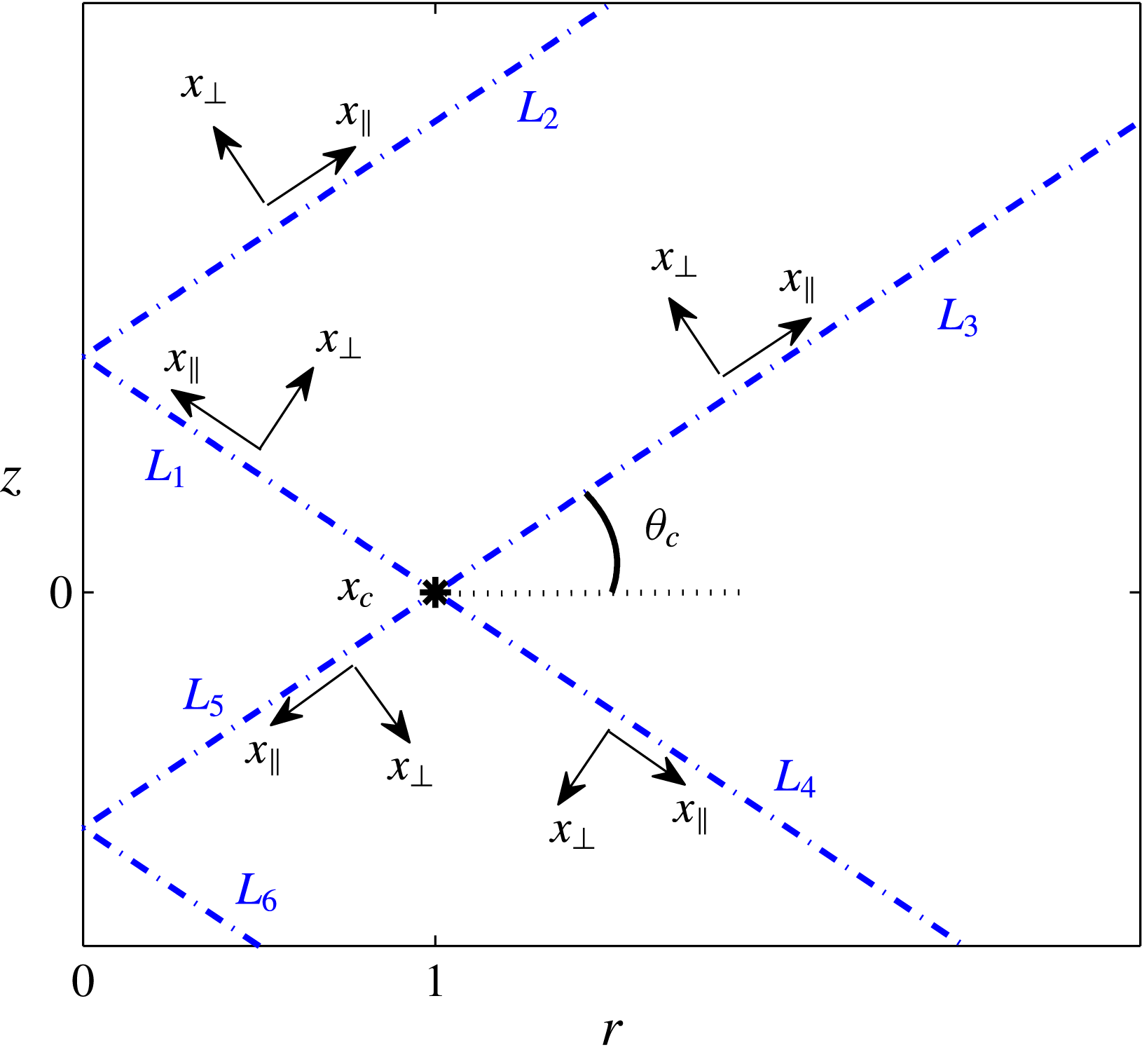
, the propagation occurs along the characteristic lines
 $L_{j}$
,
 $j=1{-}6$
, as indicated in figure 1. These lines, which actually correspond to sections of cones, make an angle
 $\unicode[STIX]{x1D703}_{c}$
, defined by (2.1), with respect to the horizontal plane. The four lines
 $L_{1}$
,
 $L_{3}$
,
 $L_{4}$
and
 $L_{5}$
are the four possible directions of emission from
 $\boldsymbol{x}_{\boldsymbol{c}}$
. The line
 $L_{2}$
(and similarly
 $L_{6}$
) is different: it is the continuation of the line
 $L_{1}$
after reflection on the axis of symmetry. Finding the properties of the similarity solution along this line is then slightly more complicated: it requires an analysis of the reflection process on the axis.
Definitions of the lines
 $L_{j}$
,
 $j=1,2,3,4,5,6$
and associated coordinate systems in the
 $(r,z)$
plane.

We therefore start by the other lines and focus on one of them:
 $L_{1}$
. Along
 $L_{1}$
, we define a local frame (
 $\boldsymbol{e}_{\Vert }$
,
 $\boldsymbol{e}_{\bot }$
) and a local coordinate system
 $(x_{\Vert },x_{\bot })$
such that
 $r\boldsymbol{e}_{r}+z\boldsymbol{e}_{z}=\boldsymbol{e}_{r}+x_{\Vert }\boldsymbol{e}_{\Vert }+x_{\bot }\boldsymbol{e}_{\bot }$
with
 $$\begin{eqnarray}\displaystyle & \boldsymbol{e}_{\Vert }=-\boldsymbol{e}_{r}\cos \unicode[STIX]{x1D703}_{c}+\boldsymbol{e}_{z}\sin \unicode[STIX]{x1D703}_{c}, & \displaystyle\end{eqnarray}$$
 $$\begin{eqnarray}\displaystyle & \boldsymbol{e}_{\bot }=\boldsymbol{e}_{r}\sin \unicode[STIX]{x1D703}_{c}+\boldsymbol{e}_{z}\cos \unicode[STIX]{x1D703}_{c}. & \displaystyle\end{eqnarray}$$
 $$\begin{eqnarray}\displaystyle & \displaystyle (-2\text{i}\cos \unicode[STIX]{x1D703}_{c}-E\unicode[STIX]{x1D6E5})v_{\Vert }=-2\cos \unicode[STIX]{x1D703}_{c}v_{\unicode[STIX]{x1D719}}-\frac{\unicode[STIX]{x2202}p}{\unicode[STIX]{x2202}x_{\Vert }}, & \displaystyle\end{eqnarray}$$
 $$\begin{eqnarray}\displaystyle & \displaystyle (-2\text{i}\cos \unicode[STIX]{x1D703}_{c}-E\unicode[STIX]{x1D6E5})v_{\bot }=2\sin \unicode[STIX]{x1D703}_{c}v_{\unicode[STIX]{x1D719}}-\frac{\unicode[STIX]{x2202}p}{\unicode[STIX]{x2202}x_{\bot }}, & \displaystyle\end{eqnarray}$$
 $$\begin{eqnarray}\displaystyle & \displaystyle (-2\text{i}\cos \unicode[STIX]{x1D703}_{c}-E\unicode[STIX]{x1D6E5})v_{\unicode[STIX]{x1D719}}=-2\sin \unicode[STIX]{x1D703}_{c}v_{\bot }+2\cos \unicode[STIX]{x1D703}_{c}v_{\Vert }, & \displaystyle\end{eqnarray}$$
 $$\begin{eqnarray}\displaystyle & \displaystyle \frac{\unicode[STIX]{x2202}v_{\bot }}{\unicode[STIX]{x2202}x_{\bot }}+\frac{\unicode[STIX]{x2202}v_{\Vert }}{\unicode[STIX]{x2202}x_{\Vert }}=2\cos \unicode[STIX]{x1D703}_{c}\frac{v_{\Vert }}{r}-2\sin \unicode[STIX]{x1D703}_{c}\frac{v_{\bot }}{r}. & \displaystyle\end{eqnarray}$$
 $\unicode[STIX]{x1D702}_{\bot }=x_{\bot }/E^{1/3}$
and the ansatz
 $$\begin{eqnarray}v_{\Vert }=\frac{u_{\Vert }^{(0)}}{\sqrt{r}},\quad v_{\bot }=E^{1/3}\frac{u_{\bot }^{(1)}}{\sqrt{r}},\quad v_{\unicode[STIX]{x1D719}}=\frac{v_{\unicode[STIX]{x1D719}}^{(0)}}{\sqrt{r}},\quad p=E^{1/3}\frac{p^{(1)}}{\sqrt{r}}\end{eqnarray}$$
we obtain the leading-order equations
 $$\begin{eqnarray}\displaystyle & v_{\unicode[STIX]{x1D719}}^{(0)}=\text{i}v_{\Vert }^{(0)}, & \displaystyle\end{eqnarray}$$
 $$\begin{eqnarray}\displaystyle & \displaystyle \frac{\unicode[STIX]{x2202}p^{(1)}}{\unicode[STIX]{x2202}\unicode[STIX]{x1D702}_{\bot }}=2\text{i}\sin \unicode[STIX]{x1D703}_{c}v_{\Vert }^{(0)}, & \displaystyle\end{eqnarray}$$
 $$\begin{eqnarray}\displaystyle & \displaystyle \frac{\unicode[STIX]{x2202}v_{\bot }^{(1)}}{\unicode[STIX]{x2202}\unicode[STIX]{x1D702}_{\bot }}=-\frac{\unicode[STIX]{x2202}v_{\Vert }^{(0)}}{\unicode[STIX]{x2202}x_{\bot }}-\cos \unicode[STIX]{x1D703}_{c}\frac{v_{\Vert }^{(0)}}{2r}, & \displaystyle\end{eqnarray}$$
 $$\begin{eqnarray}\displaystyle & \displaystyle \text{i}\frac{\unicode[STIX]{x2202}^{3}v_{\Vert }^{(0)}}{\unicode[STIX]{x2202}\unicode[STIX]{x1D702}_{\bot }^{3}}+2\sin \unicode[STIX]{x1D703}_{c}\frac{\unicode[STIX]{x2202}v_{\Vert }^{(0)}}{\unicode[STIX]{x2202}x_{\Vert }}=0. & \displaystyle\end{eqnarray}$$
Similarity solutions are obtained by searching
 $v_{\Vert }^{(0)}$
in the form
 $$\begin{eqnarray}v_{\Vert }^{(0)}=C_{0}H_{m}(x_{\Vert },\unicode[STIX]{x1D701})=C_{0}\left(\frac{x_{\Vert }}{2\sin \unicode[STIX]{x1D703}_{c}}\right)^{-m/3}h_{m}(\unicode[STIX]{x1D701}),\end{eqnarray}$$
where
 $m$
is a real number,
 $C_{0}$
a complex constant and
 $$\begin{eqnarray}\unicode[STIX]{x1D701}=\unicode[STIX]{x1D702}_{\bot }\left(\frac{2\sin \unicode[STIX]{x1D703}_{c}}{x_{\Vert }}\right)^{1/3}.\end{eqnarray}$$
The function
 $h_{m}$
is found to satisfy
 $$\begin{eqnarray}3h_{m}^{\prime \prime \prime }+\text{i}\unicode[STIX]{x1D701}h_{m}^{\prime }+\text{i}mh_{m}=0.\end{eqnarray}$$
As shown by Moore & Saffman (Reference Moore and Saffman1969), the solution which is bounded for
 $m>0$
is a multiple of
 $$\begin{eqnarray}h_{m}(\unicode[STIX]{x1D701})=\frac{\text{e}^{-\text{i}m\unicode[STIX]{x03C0}/2}}{(m-1)!}\int _{0}^{+\infty }\text{e}^{\text{i}p\unicode[STIX]{x1D701}-p^{3}}p^{m-1}\,\text{d}p.\end{eqnarray}$$
The normalization of
 $h_{m}$
has been chosen such that
 $$\begin{eqnarray}\displaystyle & & \displaystyle H_{m}(x_{\Vert },\unicode[STIX]{x1D701})~\substack{ \displaystyle \sim \\ \unicode[STIX]{x1D701}\rightarrow +\infty }~\unicode[STIX]{x1D702}_{\bot }^{-m},\end{eqnarray}$$
 $$\begin{eqnarray}\displaystyle & & \displaystyle H_{m}(x_{\Vert },\unicode[STIX]{x1D701})~\substack{ \displaystyle \sim \\ \unicode[STIX]{x1D701}\rightarrow -\infty }~(-\unicode[STIX]{x1D702}_{\bot })^{-m}\text{e}^{-\text{i}m\unicode[STIX]{x03C0}}.\end{eqnarray}$$
 $$\begin{eqnarray}v_{\unicode[STIX]{x1D719}}^{(0)}=\text{i}C_{0}H_{m}(x_{\Vert },\unicode[STIX]{x1D701}).\end{eqnarray}$$
The above analysis applies to
 $L_{1}$
. A similar analysis can be performed on the other lines
 $L_{3}$
,
 $L_{4}$
and
 $L_{5}$
. With the definition of the coordinate system shown in figure 1, we obtain the same expression (2.10) for
 $v_{\Vert }^{(0)}$
with
 $\unicode[STIX]{x1D701}$
defined by (2.11) for all these lines. However, (2.15) is valid on the lines
 $L_{1}$
and
 $L_{5}$
only. On the symmetric lines
 $L_{3}$
and
 $L_{4}$
, we must use
 $$\begin{eqnarray}v_{\unicode[STIX]{x1D719}}^{(0)}=-\text{i}C_{0}H_{m}(x_{\Vert },\unicode[STIX]{x1D701}).\end{eqnarray}$$
As shown in appendix A, on
 $L_{2}$
, we should use the formula
 $$\begin{eqnarray}v_{\Vert }^{(0)}=\text{i}C_{0}H_{m}(x_{\Vert },\unicode[STIX]{x1D701}),\quad v_{\unicode[STIX]{x1D719}}^{(0)}=C_{0}H_{m}(x_{\Vert },\unicode[STIX]{x1D701}),\end{eqnarray}$$
with
 $x_{\Vert }=(r+1)\cos \unicode[STIX]{x1D703}_{c}+z\sin \unicode[STIX]{x1D703}_{c}$
(that is counted from a symmetric source at
 $(-1,0)$
).
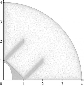
Geometry and grid of the numerical simulation, shown here for a prolate spheroid of eccentricity
 $\sqrt{2/3}$
.

2.3 Description of the numerical method
Axisymmetric direct numerical simulations are performed with the finite-element commercial software Comsol Multiphysics. Incompressible Navier–Stokes equations are solved for a Newtonian fluid in the frame of reference rotating at the mean angular velocity
 $\unicode[STIX]{x1D6FA}^{\ast }$
. The length scale in the numerics is the axis distance to the point where the characteristic line
 $L_{4}$
crosses the equator. Considering the axial and equatorial symmetries of the problem, the fluid domain then corresponds to the upper right quarter of a sphere of radius 4 (see figure 2). Boundary conditions are stress free at the spherical radial coordinate
 $\unicode[STIX]{x1D70C}=4$
, no slip with imposed libration azimuthal velocity
 $\boldsymbol{v}=\unicode[STIX]{x1D700}r\cos (\unicode[STIX]{x1D714}t)\boldsymbol{e}_{\unicode[STIX]{x1D719}}$
at the object boundary and symmetry conditions along the rotation axis. Regarding the librating disk problem, we consider 2 configurations for the boundary conditions along the equatorial plane: either
 $\boldsymbol{v}=\mathbf{0}$
, which we refer to as the ‘disk in a solid plane’ configuration, or symmetry conditions (that is
 $v_{z}=\unicode[STIX]{x2202}_{z}v_{r}=\unicode[STIX]{x2202}_{z}v_{\unicode[STIX]{x1D719}}=0$
at
 $z=0$
outside the object), which we refer to as the ‘free disk’ configuration. Symmetry conditions are also used for all the spheroidal geometries. From
 $\unicode[STIX]{x1D70C}=2$
to
 $\unicode[STIX]{x1D70C}=4$
, the viscosity increases exponentially with the radius squared by a factor of approximately 2000, so as to damp outgoing propagating waves: any wave reflected from the outer boundary is then negligible. The mesh is made of triangular standard Lagrange elements of type P3–P2 (i.e. cubic for the velocity field and quadratic for the pressure field). It is strongly refined close to the boundaries and along the characteristic lines, where rapid variations of the velocity field are expected (see figure 2). The total number of degrees of freedom ranges between 800 000 and 1.2 million, depending on the geometry of the librating object. At each time step, the system is solved with the sparse direct linear solver PARDISO and the backward difference formulae temporal solver with a maximal order 2. The time step is limited to
 $1/150$
of the libration period. No stabilization technique is used. Starting from
 $\boldsymbol{v}=\mathbf{0}$
everywhere in the fluid at time
 $t=t_{i}=-\unicode[STIX]{x03C0}/(2\unicode[STIX]{x1D714})$
, the computation is first run during 250 libration cycles so as to reach a steady state; the 5 next oscillations are then recorded and analysed. We have checked that our results are not significantly affected by changing the grid, the size of the domain, the coefficient of the viscous exponential increase or the maximum time step.
3 Libration of a disk
3.1 Summary of the asymptotic results for the disk in a solid plane
Le Dizès (Reference Le Dizès2015) provided an asymptotic expression of the solution for the librating disk in a solid plane in the limit of small Ekman numbers. In the inertial wave regime (
 $0<\unicode[STIX]{x1D714}<2$
), he found, using results by Tilgner (Reference Tilgner2000) that, outside the boundary layer on the disk (
 $z\gg \sqrt{E}$
), the velocity amplitude of the harmonic solution can be written with the present notation as
 $$\begin{eqnarray}\boldsymbol{u}=A(2\boldsymbol{u}_{D}-\boldsymbol{u}_{R}),\end{eqnarray}$$
with
 $$\begin{eqnarray}A=\frac{\sqrt{E}}{2\sin \unicode[STIX]{x1D703}_{c}}\text{e}^{\text{i}(\unicode[STIX]{x03C0}/4)-\text{i}(\unicode[STIX]{x1D703}_{c}/2)},\end{eqnarray}$$
where the two contributions
 $\boldsymbol{u}_{D}$
and
 $\boldsymbol{u}_{R}$
correspond to the solutions generated from a uniform axial oscillating forcing on the disk of unitary amplitude and from a Dirac oscillating ring source of axial flow on the disk edge, respectively. These contributions are given by
 $$\begin{eqnarray}\boldsymbol{u}_{D}=\left\{\begin{array}{@{}c@{}}u_{D}=-\text{i}{\displaystyle \frac{\cos \unicode[STIX]{x1D703}_{c}}{\sin \unicode[STIX]{x1D703}_{c}}}I_{D}^{(1)}\\ v_{D}=-{\displaystyle \frac{1}{\sin \unicode[STIX]{x1D703}_{c}}}I_{D}^{(1)}\\ w_{D}=I_{D}^{(0)}\end{array}\right.\quad \text{and}\quad \boldsymbol{u}_{R}=\left\{\begin{array}{@{}c@{}}u_{R}=-\text{i}{\displaystyle \frac{\cos \unicode[STIX]{x1D703}_{c}}{\sin \unicode[STIX]{x1D703}_{c}}}I_{R}^{(1)}\\ v_{R}=-{\displaystyle \frac{1}{\sin \unicode[STIX]{x1D703}_{c}}}I_{R}^{(1)}\\ w_{R}=I_{R}^{(0)},\end{array}\right.\end{eqnarray}$$
with
 $$\begin{eqnarray}\displaystyle & \displaystyle I_{D}^{(m)}=\int _{0}^{\infty }\text{J}_{1}(k)\text{J}_{m}(kr)\text{e}^{\text{i}k\tilde{z}}\text{e}^{-\tilde{E}k^{3}\tilde{z}}\,\text{d}k, & \displaystyle\end{eqnarray}$$
 $$\begin{eqnarray}\displaystyle & \displaystyle I_{R}^{(m)}=\int _{0}^{\infty }k\text{J}_{0}(k)\text{J}_{m}(kr)\text{e}^{\text{i}k\tilde{z}}\text{e}^{-\tilde{E}k^{3}\tilde{z}}\,\text{d}k, & \displaystyle\end{eqnarray}$$
 $$\begin{eqnarray}\tilde{z}=\frac{\cos \unicode[STIX]{x1D703}_{c}}{\sin \unicode[STIX]{x1D703}_{c}}z,\quad \tilde{E}=\frac{E}{2\cos \unicode[STIX]{x1D703}_{c}\sin ^{4}\unicode[STIX]{x1D703}_{c}}.\end{eqnarray}$$
Without the diffusing factor
 $\text{e}^{-\tilde{E}k^{3}\tilde{z}}$
the integrals
 $I_{D}^{(m)}$
and
 $I_{R}^{(m)}$
are singular on the characteristic lines
 $L_{j}$
shown in figure 1. These lines correspond to the conical structure along which the singularity at the edge of the disk propagates. Close to these lines, the functions
 $I_{D}^{(m)}$
and
 $I_{R}^{(m)}$
take a particular form as
 $E$
goes to zero. The function
 $I_{D}^{(m)}$
is
 $O(-\log (E))$
while
 $I_{R}^{(m)}$
becomes
 $O(E^{-1/3})$
. The part associated with the ring source therefore provides the dominant contribution to the solution. Close to each line, the velocity field is found to be mainly aligned along with the conical structure. The two velocity components
 $v_{\Vert }$
and
 $v_{\unicode[STIX]{x1D719}}$
(aligned along with
 $L_{j}$
and the azimuthal direction, respectively) are found to be identical albeit a phase factor. Around the line
 $L_{1}$
, Le Dizès (Reference Le Dizès2015) showed that the solution can be written as (2.8) with
 $$\begin{eqnarray}v_{\Vert }^{(0)}=-\frac{\sqrt{E}}{4\sin \unicode[STIX]{x1D703}_{c}}\text{e}^{\text{i}(\unicode[STIX]{x03C0}/4)-\text{i}(\unicode[STIX]{x1D703}_{c}/2)}\left(\frac{2\sin ^{2}\unicode[STIX]{x1D703}_{c}}{3Ez}\right)^{1/3}\boldsymbol{H}\boldsymbol{i}\left(\text{i}x_{\bot }\left(\frac{2\sin ^{2}\unicode[STIX]{x1D703}_{c}}{3Ez}\right)^{1/3}\right).\end{eqnarray}$$
If we recall that the Scorer function
 $\boldsymbol{H}\boldsymbol{i}$
can be expressed in terms of
 $h_{1}$
as
 $$\begin{eqnarray}\boldsymbol{H}\boldsymbol{i}(s)=\frac{3^{1/3}\text{i}}{\unicode[STIX]{x03C0}}h_{1}(-\text{i}3^{1/3}s)\end{eqnarray}$$
and that
 $z\sim \sin \unicode[STIX]{x1D703}_{c}x_{\Vert }$
close to
 $L_{1}$
, expression (3.6) is found to be of the form (2.10) with
 $$\begin{eqnarray}\displaystyle & m=1, & \displaystyle\end{eqnarray}$$
 $$\begin{eqnarray}\displaystyle & \displaystyle C_{0}=\frac{E^{1/6}}{4\unicode[STIX]{x03C0}\sin \unicode[STIX]{x1D703}_{c}}\text{e}^{-\text{i}(\unicode[STIX]{x03C0}/4)-\text{i}(\unicode[STIX]{x1D703}_{c}/2)}. & \displaystyle\end{eqnarray}$$
 $L_{j}$
,
 $j=2,3,4,5,6$
.
3.2 Numerical results
In this section, we provide numerical results for both the disk in a solid plane and the disk in a free space. The numerical solution is analysed after 250 periods such that transience has disappeared and a periodic regime has been reached. For the value
 $\unicode[STIX]{x1D700}=10^{-4}$
that we consider, the solution is dominated by the harmonic response. A small Ekman number
 $E=10^{-5}$
is also chosen such that the solutions can be compared to the asymptotic expressions given in the previous section. We have chosen a fixed normalized frequency
 $\unicode[STIX]{x1D714}=\sqrt{2}$
such that
 $\unicode[STIX]{x1D703}_{c}=\unicode[STIX]{x03C0}/4$
.
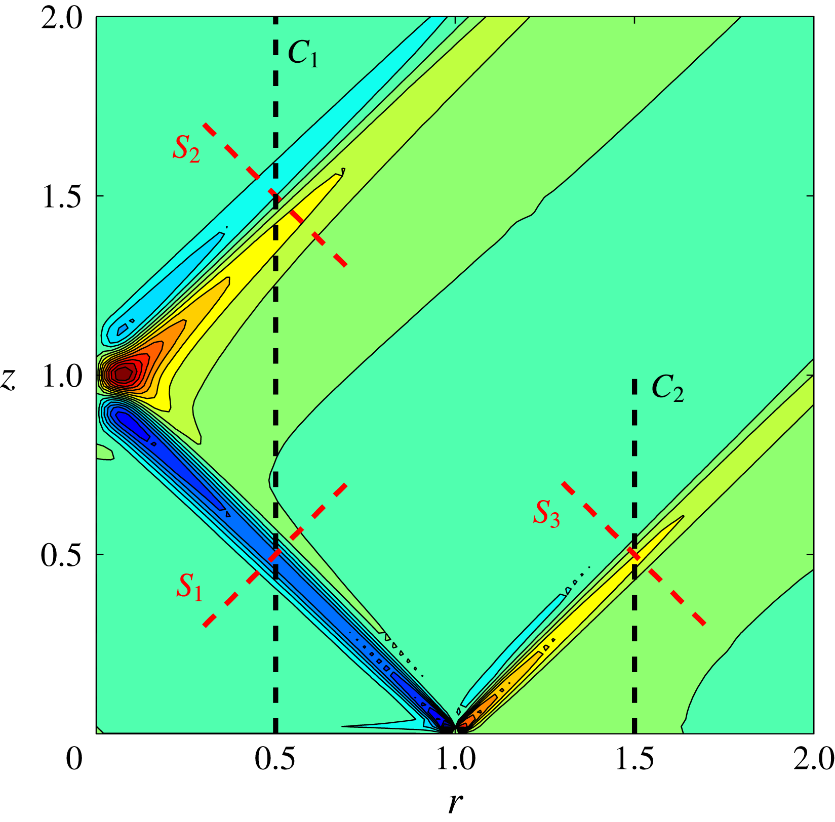
Contour of the azimuthal velocity
 $v_{\unicode[STIX]{x1D719}}$
in the
 $(r,z)$
plane of the librating disk for a disk in a solid plane configuration obtained from the numerical simulation at
 $t=501.5\unicode[STIX]{x03C0}/\unicode[STIX]{x1D714}$
for
 $E=10^{-5}$
,
 $\unicode[STIX]{x1D700}=10^{-4}$
,
 $\unicode[STIX]{x1D714}=\sqrt{2}$
. The sections
 $C_{k}$
,
 $k=1,2$
and
 $S_{j}$
,
 $j=1,2,3$
where the profiles are analysed in figures 4 and 5 are also indicated.

In figure 3, a typical contour plot of the azimuthal velocity is shown in the
 $(r,z)$
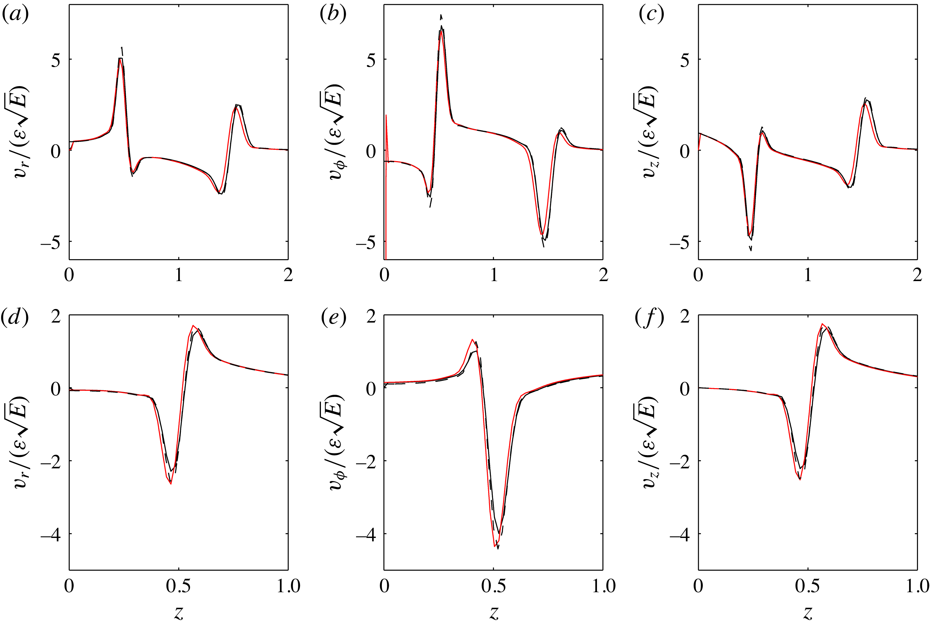
plane at a given time for the case of the free disk. In figure 4, the velocity components of the numerical solutions obtained for a free disk and for a disk in a solid plane are plotted as a function of
 $z$
in the vertical sections
 $C_{1}$
and
 $C_{2}$
corresponding to
 $r=1/2$
and
 $r=3/2$
respectively. The asymptotic solution (3.1) is also plotted in these graphs at the same instant. We can see that the free disk and the disk in a solid plane solutions are very close to each other and well described by the asymptotic solution.
Velocity profiles ((a,d)
 $v_{r}$
, (b,e)
 $v_{\unicode[STIX]{x1D719}}$
, (c,f)
 $v_{z}$
) normalized by
 $\unicode[STIX]{x1D700}\sqrt{E}$
along the vertical cut at
 $r=0.5$
(a–c) and at
 $r=1.5$
(d–f) for
 $E=10^{-5}$
,
 $\unicode[STIX]{x1D700}=10^{-4}$
,
 $\unicode[STIX]{x1D714}=\sqrt{2}$
at
 $t_{o}=508.9\unicode[STIX]{x03C0}/\unicode[STIX]{x1D714}$
. Solid lines are numerical results (in black the disk in a solid plane, in red the free disk) while dashed lines are asymptotic results for the disk in a solid plane.

Velocity profiles across the internal shear layer in the sections
 $S_{1}$
(a),
 $S_{2}$
(b) and
 $S_{3}$
(c) (see figure 3) at time
 $t_{o}=508.9\unicode[STIX]{x03C0}/\unicode[STIX]{x1D714}$
for
 $E=10^{-5}$
,
 $\unicode[STIX]{x1D700}=10^{-4}$
,
 $\unicode[STIX]{x1D714}=\sqrt{2}$
. Red (
 $v_{\unicode[STIX]{x1D719}}$
) and black (
 $v_{\Vert }$
) curves are for the disk in a solid plane, pink (
 $v_{\unicode[STIX]{x1D719}}$
) and grey (
 $v_{\Vert }$
) are for the free disk. Solid lines are numerical results. The other lines are asymptotic results. Dash-dotted lines: asymptotic formula (3.1) with ring and disk contributions. Dashed lines: similarity solution constructed using (3.8a
,
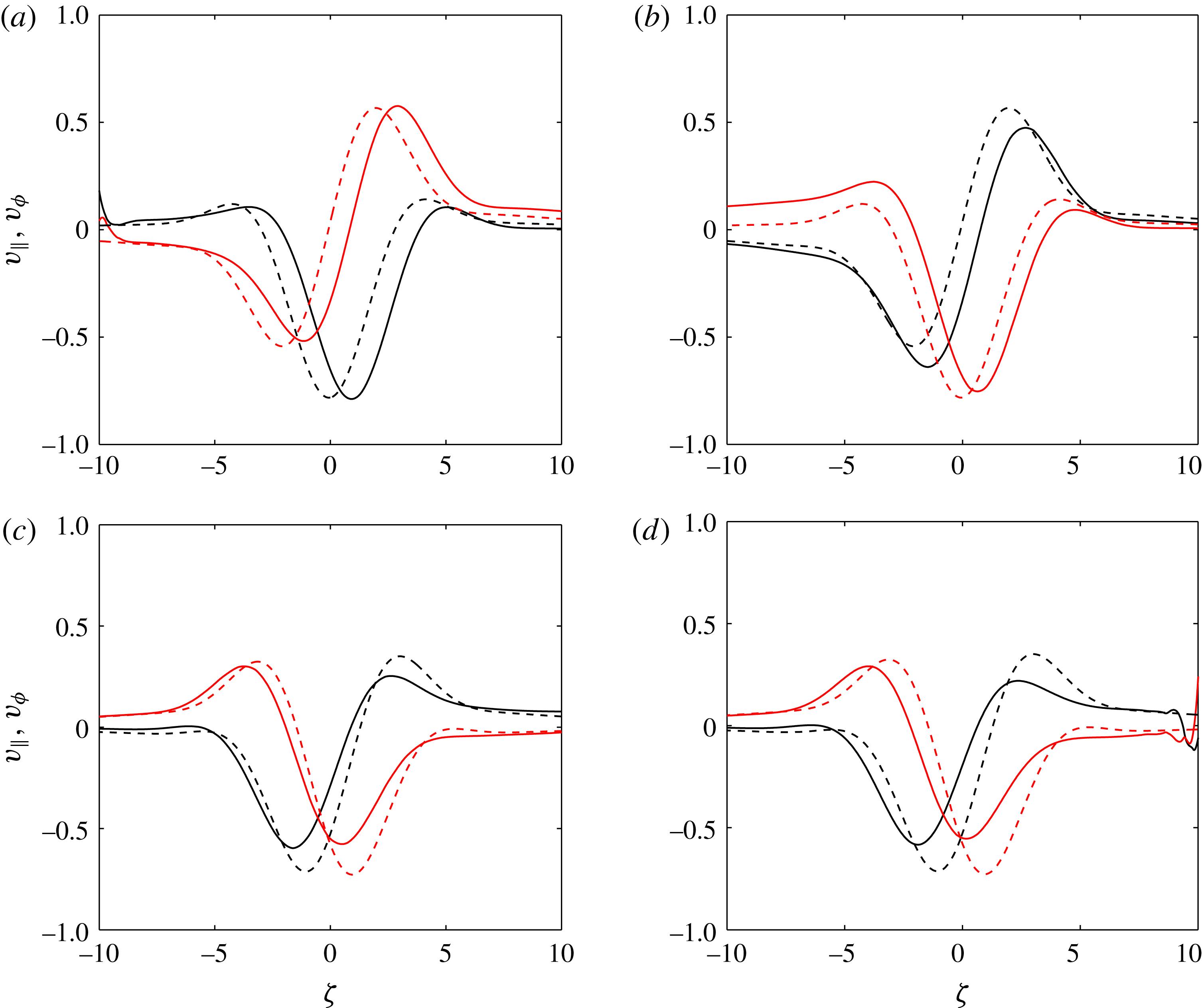
b
). All the solutions have been renormalized by the factor
 $A=\unicode[STIX]{x1D700}|C_{0}|(2\sin \unicode[STIX]{x1D703}_{c}/x_{\Vert })^{1/3}/\sqrt{r}$
with
 $C_{0}$
given by (3.8b
).

The similarity structure of the numerical solutions is also analysed in figure 5. In this figure, we plot
 $v_{\unicode[STIX]{x1D719}}$
and
 $v_{\Vert }$
, normalized by the amplitude factor
 $A=\unicode[STIX]{x1D700}|C_{0}|(2\sin \unicode[STIX]{x1D703}_{c}/x_{\Vert })^{1/3}/\sqrt{r}$
with respect to the similarity variable
 $\unicode[STIX]{x1D701}$
defined in (2.11) with the expression (3.8b
) for
 $C_{0}$
. We consider the numerical solutions in the sections
 $S_{1}$
,
 $S_{2}$
and
 $S_{3}$
indicated in figure 3 at the same time. These solutions are compared to the theoretical predictions, which can be written after the renormalization as
 $$\begin{eqnarray}V_{\Vert }^{SS}=\text{Re}(h_{1}(\unicode[STIX]{x1D701})\text{e}^{-\text{i}\unicode[STIX]{x1D711}_{\Vert }}),\quad V_{\unicode[STIX]{x1D719}}^{SS}=\text{Im}(h_{1}(\unicode[STIX]{x1D701})\text{e}^{-\text{i}\unicode[STIX]{x1D711}_{\unicode[STIX]{x1D719}}}),\end{eqnarray}$$
where
 $$\begin{eqnarray}\displaystyle & \unicode[STIX]{x1D711}_{\Vert }=\unicode[STIX]{x1D711}_{\unicode[STIX]{x1D719}}=\unicode[STIX]{x1D714}t_{o}+3\unicode[STIX]{x03C0}/8\quad \text{for}~S_{1}, & \displaystyle\end{eqnarray}$$
 $$\begin{eqnarray}\displaystyle & \unicode[STIX]{x1D711}_{\Vert }=\unicode[STIX]{x1D711}_{\unicode[STIX]{x1D719}}+\unicode[STIX]{x03C0}=\unicode[STIX]{x1D714}t_{o}-\unicode[STIX]{x03C0}/8\quad \text{for}~S_{2}, & \displaystyle\end{eqnarray}$$
 $$\begin{eqnarray}\displaystyle & \unicode[STIX]{x1D711}_{\Vert }=\unicode[STIX]{x1D711}_{\unicode[STIX]{x1D719}}+\unicode[STIX]{x03C0}=\unicode[STIX]{x1D714}t_{o}+3\unicode[STIX]{x03C0}/8\quad \text{for}~S_{3}. & \displaystyle\end{eqnarray}$$
Norm of the velocity vector along the characteristic lines
 $L_{j}$
normalized by
 $r^{-1/2}x_{\Vert }^{-1/3}$
for a libration disk in a solid plane.
 $E=10^{-5}$
,
 $\unicode[STIX]{x1D700}=10^{-4}$
,
 $\unicode[STIX]{x1D714}=\sqrt{2}$
,
 $\unicode[STIX]{x1D703}_{c}=\unicode[STIX]{x03C0}/4$
. The solid black lines are the numerical results obtained for time
 $\unicode[STIX]{x1D714}t/(2\unicode[STIX]{x03C0})=250:1/25:251$
. The dashed line is expression (3.11).

In figure 6, the solutions are analysed along the lines
 $L_{j}$
. We plot the norm of the velocity vector, normalized by
 $1/(x_{\Vert }^{1/3}\sqrt{r})$
, along the lines
 $L_{j}$
(that is for
 $x_{\bot }=0$
) as a function of
 $x_{\Vert }$
for different times. The theory predicts that this factor should be constant for all times and equal to
 $$\begin{eqnarray}|\boldsymbol{v}|x_{\Vert }^{1/3}\sqrt{r}\sim \unicode[STIX]{x1D700}|h_{1}(0)|\,|C_{0}|(2\sin \unicode[STIX]{x1D703}_{c})^{1/3}\approx 0.0895\frac{\unicode[STIX]{x1D700}E^{1/6}}{(\sin \unicode[STIX]{x1D703}_{c})^{2/3}}.\end{eqnarray}$$
This prediction has been indicated as a red dashed line in figure 6. We do observe that the numerical results follow relatively well the theoretical prediction. The departure between
 $L_{1}$
and
 $L_{2}$
corresponds to the region close to the rotation axis where the theory is known to be not applicable. We observe that the numerics provide systematically smaller values than the theory, especially on the line
 $L_{3}$
. In the future, it would be interesting to consider smaller Ekman numbers in the numerics to check that this discrepancy is indeed associated with the not sufficiently small value of the Ekman number.
4 Libration of a spheroid
In this section, we analyse the flow generated by the libration of a spheroid. We have no asymptotic solution for this geometry but we suspect that the flow structure around the characteristic rays tangent to the spheroid corresponds to one of the similarity solutions described in § 2.2. To obtain the parameter
 $m$
and the amplitude factor
 $C_{0}$
of the solution, we perform an asymptotic analysis close to the critical latitude
 $\boldsymbol{x}_{\boldsymbol{c}}$
. More precisely, these parameters are obtained by the condition of matching close to
 $\boldsymbol{x}_{\boldsymbol{c}}$
of the boundary layer solution on the object with the similarity solution. The theoretical result is then tested and validated using direct numerical simulations.
4.1 Asymptotic analysis close to
 $\boldsymbol{x}_{\boldsymbol{c}}$

4.1.1 Boundary layer solution
In this section, we consider an arbitrary axisymmetric convex object librating and rotating around its axis of symmetry
 $Oz$
. We analyse the solution in a plane
 $\unicode[STIX]{x1D6F4}$
containing this axis
 $Oz$
. In this plane, we assume that the object surface is described by a smooth curve
 $(r(s),z(s))$
, with tangential and normal vectors defined by
 $$\begin{eqnarray}\boldsymbol{t}=\frac{r^{\prime }\boldsymbol{e}_{\boldsymbol{r}}+z^{\prime }\boldsymbol{e}_{\boldsymbol{z}}}{\unicode[STIX]{x1D6FC}},\quad \boldsymbol{n}=\frac{-z^{\prime }\boldsymbol{e}_{\boldsymbol{r}}+r^{\prime }\boldsymbol{e}_{\boldsymbol{z}}}{\unicode[STIX]{x1D6FC}},\end{eqnarray}$$
with
 $$\begin{eqnarray}\unicode[STIX]{x1D6FC}=\sqrt{r^{\prime 2}+z^{\prime 2}},\end{eqnarray}$$
where the prime denotes derivative with respect to
 $s$
. The surface being convex, any point
 $M(\unicode[STIX]{x1D709},\unicode[STIX]{x1D712})$
in the fluid (outside the object) is identified by a curvilinear abscissa
 $s$
and a distance
 $x_{n}$
to the surface such that
 $\mathit{OM}=\unicode[STIX]{x1D709}\boldsymbol{e}_{\boldsymbol{r}}+\unicode[STIX]{x1D712}\boldsymbol{e}_{\boldsymbol{z}}=r(s)\boldsymbol{e}_{\boldsymbol{r}}+z(s)\boldsymbol{e}_{\boldsymbol{z}}+x_{n}\boldsymbol{n}$
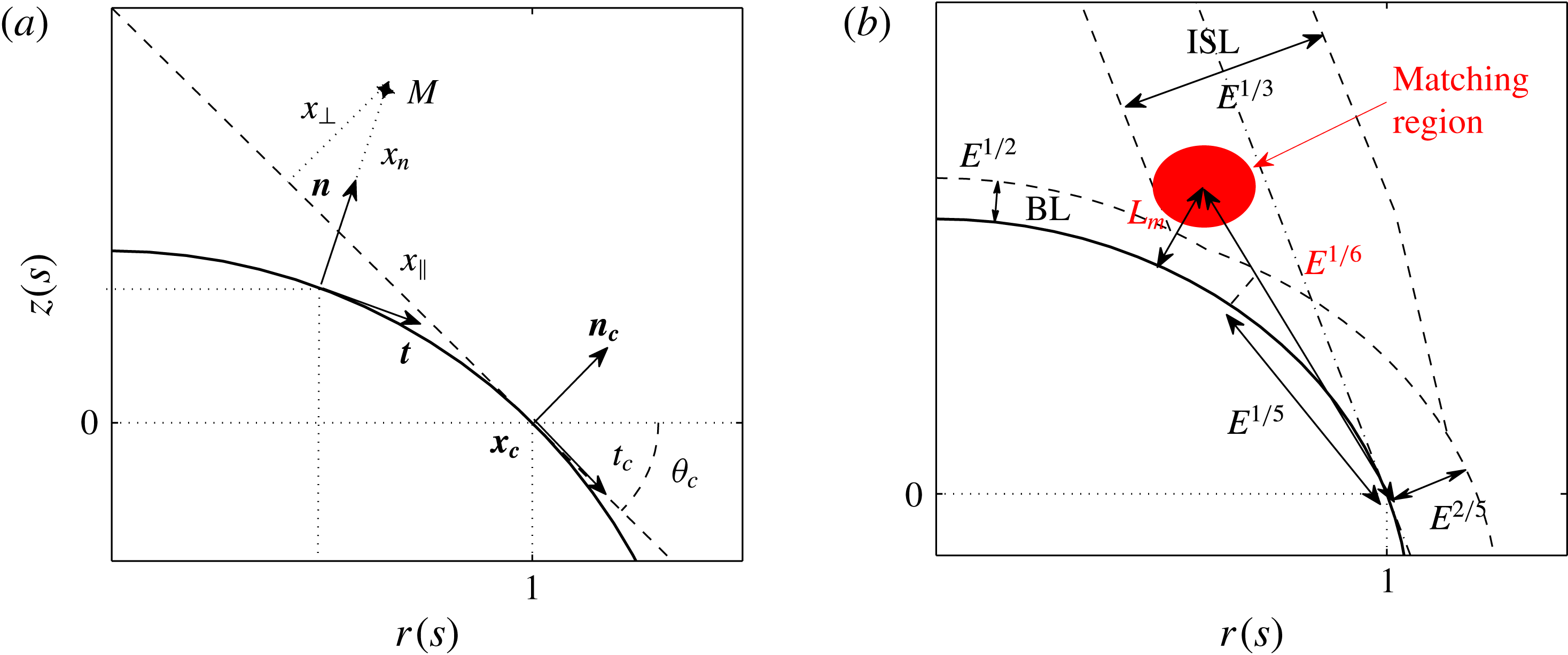
(see figure 7
a). We assume that the critical latitude
 $\boldsymbol{x}_{\boldsymbol{c}}$
on the surface is reached at
 $s=s_{c}$
. At such a point, the tangential and normal vectors are given by
 $$\begin{eqnarray}\boldsymbol{t}_{c}=\cos \unicode[STIX]{x1D703}_{c}\boldsymbol{e}_{\boldsymbol{r}}-\sin \unicode[STIX]{x1D703}_{c}\boldsymbol{e}_{\boldsymbol{z}},\quad \boldsymbol{n}_{c}=\sin \unicode[STIX]{x1D703}_{c}\boldsymbol{e}_{\boldsymbol{r}}+\cos \unicode[STIX]{x1D703}_{c}\boldsymbol{e}_{\boldsymbol{z}}.\end{eqnarray}$$
We therefore have the following equalities:
 $$\begin{eqnarray}r(s_{c})=r_{c}=1,\quad z(s_{c})=z_{c}=0,\end{eqnarray}$$
 $$\begin{eqnarray}r^{\prime }(s_{c})=r_{c}^{\prime }=\unicode[STIX]{x1D6FC}_{c}\cos \unicode[STIX]{x1D703}_{c},\quad z^{\prime }(s_{c})=z_{c}^{\prime }=-\unicode[STIX]{x1D6FC}_{c}\sin \unicode[STIX]{x1D703}_{c}.\end{eqnarray}$$
(a) Definition of the coordinate systems near
 $\boldsymbol{x}_{\boldsymbol{c}}$
. (b) Sketch of the different regions of the asymptotic analysis. The region of matching is at
 $O(E^{1/6})$
from
 $\boldsymbol{x}_{\boldsymbol{c}}$
within the internal shear layer (ISL) but outside the boundary layer (BL), i.e. at a distance
 $L_{m}$
from the boundary satisfying
 $E^{5/12}\ll L_{m}\ll E^{1/3}$
.

Introducing the boundary layer variable
 $\unicode[STIX]{x1D702}=x_{n}/\sqrt{E}$
and the following ansatz for the pressure and velocity components along
 $\boldsymbol{t}$
,
 $\boldsymbol{n}$
and
 $\boldsymbol{e}_{\unicode[STIX]{x1D719}}$
:
 $$\begin{eqnarray}p=\sqrt{E}\bar{p}^{(1)}(s,\unicode[STIX]{x1D702}),\quad v_{t}=\bar{v}_{t}^{(0)}(s,\unicode[STIX]{x1D702}),\quad v_{n}=\sqrt{E}\bar{v}_{n}^{(1)}(s,\unicode[STIX]{x1D702}),\quad v_{\unicode[STIX]{x1D719}}=\bar{v}_{\unicode[STIX]{x1D719}}^{(0)}(s,\unicode[STIX]{x1D702}),\end{eqnarray}$$
 $$\begin{eqnarray}\displaystyle & \displaystyle \left(-2\text{i}\cos \unicode[STIX]{x1D703}_{c}-\frac{\unicode[STIX]{x2202}^{2}}{\unicode[STIX]{x2202}\unicode[STIX]{x1D702}^{2}}\right)\bar{v}_{t}^{(0)}-2\frac{r^{\prime }}{\unicode[STIX]{x1D6FC}}\bar{v}_{\unicode[STIX]{x1D719}}^{(0)}=0, & \displaystyle\end{eqnarray}$$
 $$\begin{eqnarray}\displaystyle & \displaystyle \left(-2\text{i}\cos \unicode[STIX]{x1D703}_{c}-\frac{\unicode[STIX]{x2202}^{2}}{\unicode[STIX]{x2202}\unicode[STIX]{x1D702}^{2}}\right)\bar{v}_{\unicode[STIX]{x1D719}}^{(0)}+2\frac{r^{\prime }}{\unicode[STIX]{x1D6FC}}\bar{v}_{t}^{(0)}=0, & \displaystyle\end{eqnarray}$$
 $$\begin{eqnarray}\displaystyle & \displaystyle 2\frac{z^{\prime }}{\unicode[STIX]{x1D6FC}}\bar{v}_{\unicode[STIX]{x1D719}}^{(0)}=\frac{\unicode[STIX]{x2202}\bar{p}^{(1)}}{\unicode[STIX]{x2202}\unicode[STIX]{x1D702}}, & \displaystyle\end{eqnarray}$$
 $$\begin{eqnarray}\displaystyle & \displaystyle \frac{\unicode[STIX]{x2202}\bar{v}_{n}^{(1)}}{\unicode[STIX]{x2202}\unicode[STIX]{x1D702}}+\frac{1}{\unicode[STIX]{x1D6FC}}\frac{\unicode[STIX]{x2202}\bar{v}_{t}^{(0)}}{\unicode[STIX]{x2202}s}+\frac{r^{\prime }}{r\unicode[STIX]{x1D6FC}}\bar{v}_{t}^{(0)}=0. & \displaystyle\end{eqnarray}$$
 $$\begin{eqnarray}\displaystyle & \displaystyle \bar{v}_{\unicode[STIX]{x1D719}}^{(0)}=\frac{r(s)}{2}(\text{e}^{-\unicode[STIX]{x1D706}_{-}\unicode[STIX]{x1D702}}+\text{e}^{-\unicode[STIX]{x1D706}_{+}\unicode[STIX]{x1D702}}), & \displaystyle\end{eqnarray}$$
 $$\begin{eqnarray}\displaystyle & \displaystyle \bar{v}_{t}^{(0)}=\frac{\text{i}r(s)}{2}(\text{e}^{-\unicode[STIX]{x1D706}_{-}\unicode[STIX]{x1D702}}-\text{e}^{-\unicode[STIX]{x1D706}_{+}\unicode[STIX]{x1D702}}), & \displaystyle\end{eqnarray}$$
 $$\begin{eqnarray}\unicode[STIX]{x1D706}_{\pm }=\sqrt{-2\text{i}\left(\cos \unicode[STIX]{x1D703}_{c}\pm \frac{r^{\prime }}{\unicode[STIX]{x1D6FC}}\right)}\end{eqnarray}$$
are such that
 $\text{Re}(\unicode[STIX]{x1D706}_{\pm })>0$
. The third equation (4.6c
) can be used to get the pressure field, while (4.6d
) gives
 $$\begin{eqnarray}\displaystyle \bar{v}_{n}^{(1)} & = & \displaystyle \frac{\text{i}r(s)\unicode[STIX]{x1D702}}{2\unicode[STIX]{x1D6FC}}\left(\frac{\unicode[STIX]{x1D706}_{+}^{\prime }}{\unicode[STIX]{x1D706}_{+}}\text{e}^{-\unicode[STIX]{x1D706}_{+}\unicode[STIX]{x1D702}}-\frac{\unicode[STIX]{x1D706}_{-}^{\prime }}{\unicode[STIX]{x1D706}_{-}}\text{e}^{-\unicode[STIX]{x1D706}_{-}\unicode[STIX]{x1D702}}\right)+\left(\frac{\text{i}r^{\prime }}{2\unicode[STIX]{x1D6FC}\unicode[STIX]{x1D706}_{-}}-\frac{\text{i}r\unicode[STIX]{x1D706}_{-}^{\prime }}{2\unicode[STIX]{x1D6FC}\unicode[STIX]{x1D706}_{-}^{2}}\right)(\text{e}^{-\unicode[STIX]{x1D706}_{-}\unicode[STIX]{x1D702}}-1)\nonumber\\ \displaystyle & & \displaystyle -\left(\frac{\text{i}r^{\prime }}{2\unicode[STIX]{x1D6FC}\unicode[STIX]{x1D706}_{+}}-\frac{\text{i}r\unicode[STIX]{x1D706}_{+}^{\prime }}{2\unicode[STIX]{x1D6FC}\unicode[STIX]{x1D706}_{+}^{2}}\right)(\text{e}^{-\unicode[STIX]{x1D706}_{+}\unicode[STIX]{x1D702}}-1).\end{eqnarray}$$
This last expression can be used to obtain the Ekman pumping in the bulk. We are especially interested in its expression close to
 $\boldsymbol{x}_{\boldsymbol{c}}$
when
 $s$
goes to
 $s_{c}$
. Here we consider the situation illustrated in figure 7(b), which corresponds to
 $L_{1}$
. For this case,
 $s$
is always smaller than
 $s_{c}$
. Close to
 $s_{c}$
,
 $\unicode[STIX]{x1D706}_{+}$
remains finite but
 $\unicode[STIX]{x1D706}_{-}$
goes to zero as
 $$\begin{eqnarray}\unicode[STIX]{x1D706}_{-}\sim (1+\text{i})\sqrt{-\unicode[STIX]{x1D705}_{c}\unicode[STIX]{x1D6FC}_{c}\sin \unicode[STIX]{x1D703}_{c}(s_{c}-s)},\end{eqnarray}$$
where
 $\unicode[STIX]{x1D705}_{c}$
is the local curvature at
 $\boldsymbol{x}_{\boldsymbol{c}}$
. The curvature
 $\unicode[STIX]{x1D705}$
is defined by
 $$\begin{eqnarray}\unicode[STIX]{x1D705}=\frac{z^{\prime \prime }r^{\prime }-r^{\prime \prime }z^{\prime }}{\unicode[STIX]{x1D6FC}^{3}}.\end{eqnarray}$$
Here, it is negative in the neighbourhood of
 $\boldsymbol{x}_{\boldsymbol{c}}$
.
If we perform the limits
 $\unicode[STIX]{x1D702}\rightarrow \infty$
(first) and
 $s\rightarrow s_{c}$
(second), we get a normal velocity which behaves as
 $$\begin{eqnarray}v_{n}\sim \frac{(1+\text{i})}{8\unicode[STIX]{x1D6FC}_{c}^{3/2}\sqrt{-\unicode[STIX]{x1D705}_{c}\sin \unicode[STIX]{x1D703}_{c}}}\frac{\sqrt{E}}{(s_{c}-s)^{3/2}}.\end{eqnarray}$$
This limit is valid as long as
 $\unicode[STIX]{x1D702}\sqrt{s_{c}-s}\rightarrow \infty$
when
 $s\rightarrow s_{c}$
.
4.1.2 Similarity solution near
$\boldsymbol{x}_{\boldsymbol{c}}$

The similarity solutions introduced in § 2.2 are singular as we get close to
 $\boldsymbol{x}_{\boldsymbol{c}}$
. For a fixed
 $\unicode[STIX]{x1D702}_{\bot }$
, this amounts to considering the limit
 $x_{\Vert }\rightarrow 0$
. As we are interested in the solution close to the boundary for
 $L_{1}$
, we consider a negative
 $\unicode[STIX]{x1D702}_{\bot }$
(see figure 7
b) such that
 $\unicode[STIX]{x1D701}$
defined by (2.11) goes to
 $-\infty$
as
 $x_{\Vert }\rightarrow 0$
. In this limit, we obtain
 $$\begin{eqnarray}\displaystyle & v_{\Vert }\sim C_{0}(-\unicode[STIX]{x1D702}_{\bot })^{-m}\text{e}^{-\text{i}m\unicode[STIX]{x03C0}}, & \displaystyle\end{eqnarray}$$
 $$\begin{eqnarray}\displaystyle & \displaystyle v_{\bot }\sim -C_{0}E^{1/3}\frac{\cos \unicode[STIX]{x1D703}_{c}}{2(m-1)}(-\unicode[STIX]{x1D702}_{\bot })^{-m+1}\text{e}^{-\text{i}m\unicode[STIX]{x03C0}}. & \displaystyle\end{eqnarray}$$
 $-\unicode[STIX]{x1D702}_{\bot }(x_{\Vert })^{-1/3}\gg 1$
.
4.1.3 Matching
In this section, we show that the similarity solution and the boundary layer solution are compatible for particular values of
 $C_{0}$
and
 $m$
. The matching is performed in the region where both expressions (4.12) and (4.13) apply. To determine this region, it is useful to express the variables
 $x_{\Vert }$
and
 $\unicode[STIX]{x1D702}_{\bot }$
in terms of the boundary layer variables
 $s$
and
 $\unicode[STIX]{x1D702}$
:
 $$\begin{eqnarray}\displaystyle & \displaystyle x_{\Vert }=-\cos \,\unicode[STIX]{x1D703}_{c}\left(r(s)-1-\sqrt{E}\unicode[STIX]{x1D702}\frac{z^{\prime }}{\unicode[STIX]{x1D6FC}}\right)+\sin \unicode[STIX]{x1D703}_{c}\left(z(s)+\sqrt{E}\unicode[STIX]{x1D702}\frac{r^{\prime }}{\unicode[STIX]{x1D6FC}}\right), & \displaystyle\end{eqnarray}$$
 $$\begin{eqnarray}\displaystyle & \displaystyle \unicode[STIX]{x1D702}_{\bot }=\frac{\sin \unicode[STIX]{x1D703}_{c}}{E^{1/3}}\left(r(s)-1-\sqrt{E}\unicode[STIX]{x1D702}\frac{z^{\prime }}{\unicode[STIX]{x1D6FC}}\right)+\frac{\cos \unicode[STIX]{x1D703}_{c}}{E^{1/3}}\left(z(s)+\sqrt{E}\unicode[STIX]{x1D702}\frac{r^{\prime }}{\unicode[STIX]{x1D6FC}}\right). & \displaystyle\end{eqnarray}$$
 $\boldsymbol{x}_{\boldsymbol{c}}$
, these expressions become
 $$\begin{eqnarray}\displaystyle & x_{\Vert }\sim \unicode[STIX]{x1D6FC}_{c}(s_{c}-s)+\sqrt{E}\unicode[STIX]{x1D705}_{c}\unicode[STIX]{x1D6FC}_{c}\unicode[STIX]{x1D702}(s_{c}-s), & \displaystyle\end{eqnarray}$$
 $$\begin{eqnarray}\displaystyle & \displaystyle \unicode[STIX]{x1D702}_{\bot }\sim E^{1/6}\unicode[STIX]{x1D702}+E^{-1/3}\unicode[STIX]{x1D705}_{c}\unicode[STIX]{x1D6FC}_{c}^{2}\frac{(s_{c}-s)^{2}}{2}, & \displaystyle\end{eqnarray}$$
 $\unicode[STIX]{x1D705}_{c}$
is the curvature at
 $\boldsymbol{x}_{\boldsymbol{c}}$
.
If
 $|s-s_{c}|=O(E^{1/6})$
and
 $E^{-1/12}\ll \unicode[STIX]{x1D702}\ll E^{-1/6}$
, we do have
 $\sqrt{|s-s_{c}|}\unicode[STIX]{x1D702}\gg 1$
as required by (4.12). Moreover, we then obtain
 $$\begin{eqnarray}\displaystyle & x_{\Vert }\sim \unicode[STIX]{x1D6FC}_{c}(s_{c}-s), & \displaystyle\end{eqnarray}$$
 $$\begin{eqnarray}\displaystyle & \displaystyle \unicode[STIX]{x1D702}_{\bot }\sim E^{-1/3}\unicode[STIX]{x1D705}_{c}\unicode[STIX]{x1D6FC}_{c}^{2}\frac{(s-s_{c})^{2}}{2}, & \displaystyle\end{eqnarray}$$
 $-\unicode[STIX]{x1D702}_{\bot }x_{\Vert }^{-1/3}\propto E^{-1/3}(s_{c}-s)^{5/3}=O(E^{-1/18})\gg 1$
as required for the validity of (4.13). This region is materialized in red in the sketch shown in figure 7(b). In this figure, we have also indicated the scalings of the different asymptotic regions: the
 $O(E^{1/2})$
width of the boundary layer on the object far from
 $s_{c}$
, the
 $O(E^{1/3})$
width of the similarity solution around
 $L_{1}$
far from
 $s_{c}$
, and the scalings in
 $E^{1/5}$
and
 $E^{2/5}$
of the local region near
 $s_{c}$
where the singularities of both the boundary layer solution and the similarity solution are smoothed (Roberts & Stewartson Reference Roberts and Stewartson1963; Kerswell Reference Kerswell1995).
In this region, we can then match the boundary layer solution with the similarity solution. The normal velocity
 $v_{n}$
can be deduced from
 $v_{\Vert }$
and
 $v_{\bot }$
using
 $$\begin{eqnarray}v_{n}=\frac{1}{\unicode[STIX]{x1D6FC}}((z^{\prime }\cos \unicode[STIX]{x1D703}_{c}+r^{\prime }\sin \unicode[STIX]{x1D703}_{c})v_{\Vert }+(-z^{\prime }\sin \unicode[STIX]{x1D703}_{c}+r^{\prime }\cos \unicode[STIX]{x1D703}_{c})v_{\bot }),\end{eqnarray}$$
which becomes close to
 $s_{c}$
 $$\begin{eqnarray}v_{n}\sim v_{\bot }-\unicode[STIX]{x1D705}_{c}\unicode[STIX]{x1D6FC}_{c}(s_{c}-s)v_{\Vert }.\end{eqnarray}$$
If we take into account (4.16a , b ), the normal velocity obtained from the similarity solution (4.13a , b ) is therefore
 $$\begin{eqnarray}v_{n}\sim E^{m/3}(-\unicode[STIX]{x1D705}_{c})^{-m+1}2^{m}\unicode[STIX]{x1D6FC}_{c}^{-2m+1}(s_{c}-s)^{-2m+1}C_{0}\text{e}^{-\text{i}m\unicode[STIX]{x03C0}}.\end{eqnarray}$$
This expression is compatible with (4.12) if and only if
 $$\begin{eqnarray}\displaystyle & m=5/4, & \displaystyle\end{eqnarray}$$
 $$\begin{eqnarray}\displaystyle & \displaystyle C_{0}=\frac{E^{1/12}}{8\sqrt{2\sin \unicode[STIX]{x1D703}_{c}}(-2\unicode[STIX]{x1D705}_{c})^{1/4}}\text{e}^{-\text{i}\unicode[STIX]{x03C0}/2}. & \displaystyle\end{eqnarray}$$
These expressions for
 $m$
and
 $C_{0}$
apply for the similarity solution along the line
 $L_{1}$
. A similar analysis can be carried out for the similarity solution along
 $L_{4}$
by performing the matching on the other side of
 $\boldsymbol{x}_{\boldsymbol{c}}$
. It gives the same value of
 $m$
and an amplitude
 $C_{0}$
just differing by a phase factor:
 $$\begin{eqnarray}C_{0}=\frac{E^{1/12}}{8\sqrt{2\sin \unicode[STIX]{x1D703}_{c}}(-2\unicode[STIX]{x1D705}_{c})^{1/4}}\text{e}^{-\text{i}\unicode[STIX]{x03C0}/4}.\end{eqnarray}$$
These values of
 $m$
and
 $C_{0}$
constitute the main result of the present paper. In particular, it is worth mentioning that the value of
 $m$
is larger for a smooth surface (spheroid) than for an angular one (disk). This means that we have the following counter-intuitive result: the similarity solution describing the internal shear layer is associated with a stronger singularity at
 $\boldsymbol{x}_{\boldsymbol{c}}$
for a smooth surface than for an angular one. As a consequence, the amplitude of the velocity field is larger for the spheroid with a scaling in
 $E^{1/12}$
to be compared with the
 $E^{1/6}$
scaling for the disk. Expressions (4.20b
) and (4.21) provide the dependency with respect to the libration frequency through the term
 $2\sin \unicode[STIX]{x1D703}_{c}=\sqrt{4-\unicode[STIX]{x1D714}^{2}}$
. The amplitude of the internal shear layer increases when
 $\unicode[STIX]{x1D703}_{c}$
decreases, that is when
 $\unicode[STIX]{x1D714}$
gets close to 2 (or
 $\unicode[STIX]{x1D714}^{\ast }$
close to
 $2\unicode[STIX]{x1D6FA}^{\ast }$
). We can also note the dependency with respect to the local curvature
 $\unicode[STIX]{x1D705}_{c}$
. The amplitude decreases as
 $|\unicode[STIX]{x1D705}_{c}|$
increases. The more peaky the surface at
 $\boldsymbol{x}_{\boldsymbol{c}}$
is, the smaller the amplitude of the internal shear layer is. This is consistent with the smaller amplitude scaling obtained for the singular case of the disk.
4.2 Comparison with numerical results
In this section, the formulas (4.20a , b ) are tested against direct numerical simulations. Different spheroids as well as different frequencies are considered.
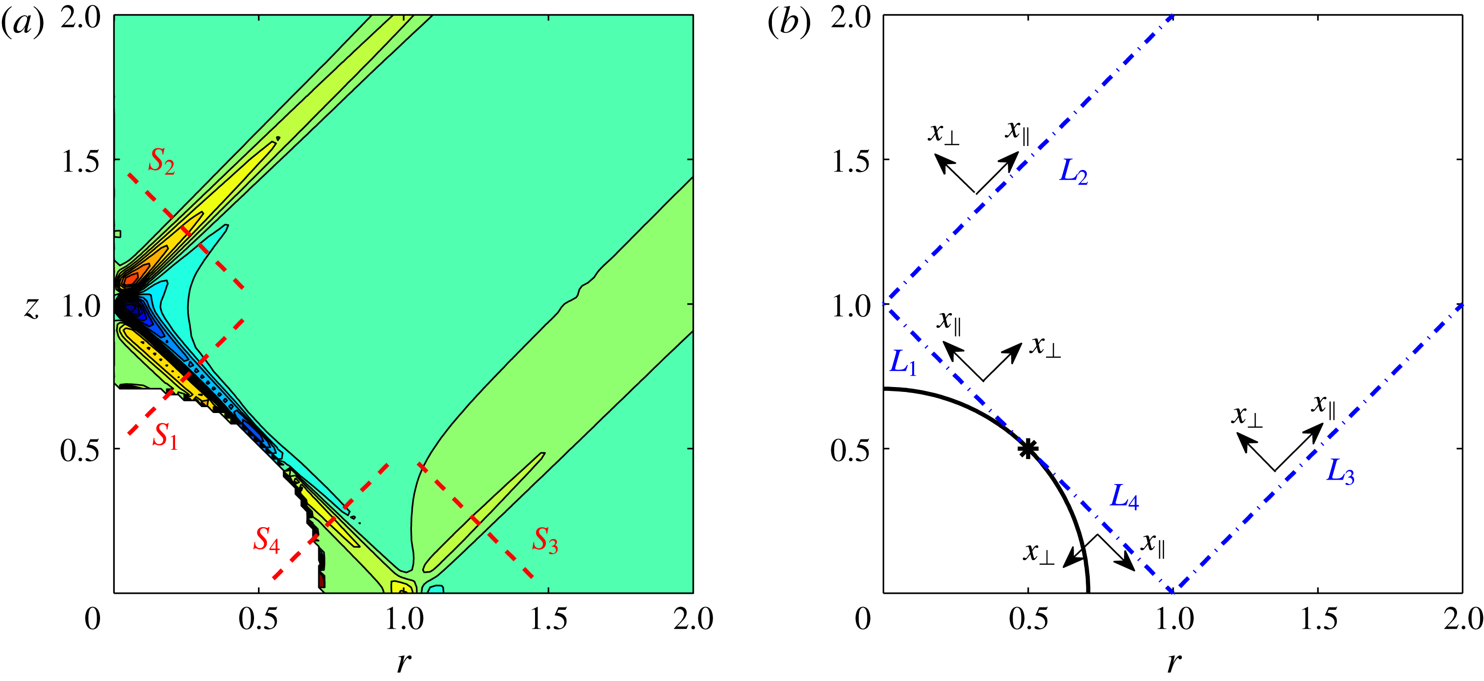
(a) Contour of the azimuthal velocity
 $v_{\unicode[STIX]{x1D719}}$
in the
 $(r,z)$
plane of a librating sphere obtained from the numerical simulation at time
 $t=508.9\unicode[STIX]{x03C0}/\unicode[STIX]{x1D714}$
for
 $E_{s}=10^{-5}$
,
 $\unicode[STIX]{x1D700}=10^{-4}$
,
 $\unicode[STIX]{x1D714}=\sqrt{2}$
. The sections
 $S_{j}$
,
 $j=1,2,3,4$
, where the profiles are analysed in figure 9, are also indicated. (b) Definition of the local coordinate system on the characteristic lines
 $L_{j}$
,
 $j=1,2,3,4$
. The star indicates the source point of the similarity solutions.

The numerical simulations were first performed for a sphere of radius
 $1/\sqrt{2}$
with a frequency
 $\unicode[STIX]{x1D714}=\sqrt{2}$
such that the singular rays start from the point
 $\boldsymbol{x}_{\boldsymbol{c}}=(1/2,1/2)$
on the surface and cross the meridional plane and the rotation axis at
 $(1,0)$
and
 $(0,1)$
respectively, as illustrated in figure 8(a). This normalization does not correspond to that chosen for the similarity solution. The Ekman number of the simulation
 $E_{s}$
is therefore 4 times smaller than the Ekman number defined in (2.2). The internal shear layers are emitted on either side of
 $\boldsymbol{x}_{\boldsymbol{c}}$
along the lines
 $L_{1}$
and
 $L_{4}$
indicated in figure 8(b). The internal shear layer on
 $L_{1}$
is reflected on the axis and continues along
 $L_{2}$
. The internal shear layer on
 $L_{3}$
corresponds to that emitted from the symmetric point
 $(1/2,-1/2)$
on the sphere. The definition of the coordinate systems is given in figure 8(b), in agreement with the definition used in figure 1.
Profiles of
 $v_{\unicode[STIX]{x1D719}}$
(red curves) and
 $v_{\Vert }$
(black curves) across the internal shear layer in the sections
 $S_{1}$
(a),
 $S_{2}$
(b),
 $S_{3}$
(c) and
 $S_{4}$
(d) as indicated in figure 8, at time
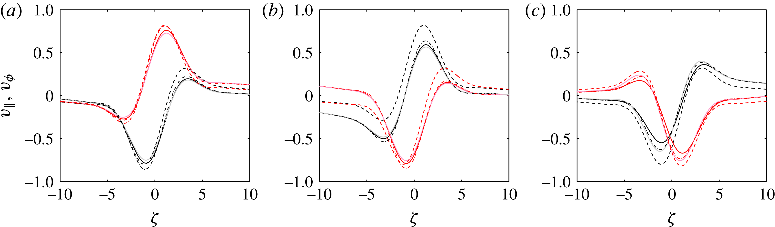
 $t=508.9\unicode[STIX]{x03C0}/\unicode[STIX]{x1D714}$
for
 $E_{s}=2.5\times 10^{-6}$
(i.e.
 $E=10^{-5}$
),
 $\unicode[STIX]{x1D700}=10^{-4}$
,
 $\unicode[STIX]{x1D714}=\sqrt{2}$
. Solid lines are numerical results. Dashed lines are the similarity solutions. All the solutions have been renormalized by the factor
 $A=\unicode[STIX]{x1D700}|C_{0}|(2\sin \unicode[STIX]{x1D703}_{c}/x_{\Vert })^{5/4}/\sqrt{r}$
with
 $C_{0}$
given by (4.20b
) or (4.21).

In figure 9, we compare the numerical solution to the similarity solution in the sections indicated in figure 8(a) at a particular instant. Both the azimuthal velocity and the parallel velocity are plotted as a function of the similarity variable. As for the disk, the normalization has been chosen such that the theoretical predications for
 $v_{\unicode[STIX]{x1D719}}$
and
 $v_{\Vert }$
are just given by
 $$\begin{eqnarray}V_{\Vert }^{SS}=\text{Re}(h_{5/4}(\unicode[STIX]{x1D701})\text{e}^{-\text{i}\unicode[STIX]{x1D711}_{\Vert }}),\quad V_{\unicode[STIX]{x1D719}}^{SS}=\text{Im}(h_{5/4}(\unicode[STIX]{x1D701})\text{e}^{-\text{i}\unicode[STIX]{x1D711}_{\unicode[STIX]{x1D719}}}),\end{eqnarray}$$
where
 $$\begin{eqnarray}\displaystyle & \unicode[STIX]{x1D711}_{\Vert }=\unicode[STIX]{x1D711}_{\unicode[STIX]{x1D719}}=\unicode[STIX]{x1D714}t_{o}+\unicode[STIX]{x03C0}/2\quad \text{for}~S_{1}, & \displaystyle\end{eqnarray}$$
 $$\begin{eqnarray}\displaystyle & \unicode[STIX]{x1D711}_{\Vert }=\unicode[STIX]{x1D711}_{\unicode[STIX]{x1D719}}+\unicode[STIX]{x03C0}=\unicode[STIX]{x1D714}t_{o}\quad \text{for}~S_{2}, & \displaystyle\end{eqnarray}$$
 $$\begin{eqnarray}\displaystyle & \unicode[STIX]{x1D711}_{\Vert }=\unicode[STIX]{x1D711}_{\unicode[STIX]{x1D719}}+\unicode[STIX]{x03C0}=\unicode[STIX]{x1D714}t_{o}+\unicode[STIX]{x03C0}/4\quad \text{for}~S_{3}~\text{and}~S_{4}. & \displaystyle\end{eqnarray}$$
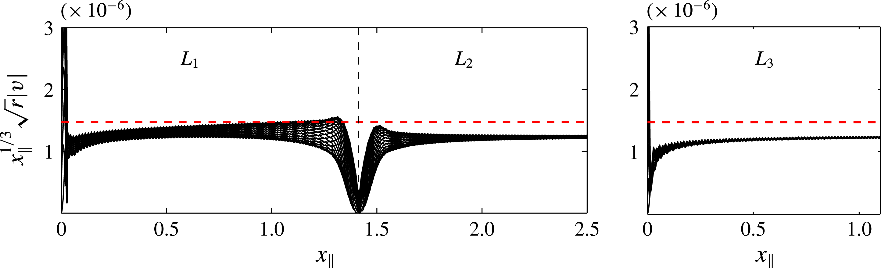
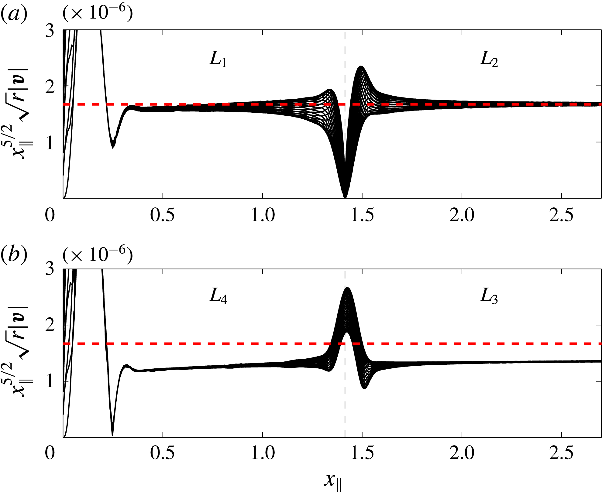
Norm of the velocity vector along the characteristic lines
 $L_{j}$
normalized by
 $x_{\Vert }^{-5/2}r^{-1/2}$
for a librating sphere with
 $E_{s}=2.5\times 10^{-6}$
(i.e.
 $E=10^{-5}$
),
 $\unicode[STIX]{x1D700}=10^{-4}$
,
 $\unicode[STIX]{x1D714}=\sqrt{2}$
,
 $\unicode[STIX]{x1D703}_{c}=\unicode[STIX]{x03C0}/4$
. The solid black lines are the numerical results obtained for time
 $\unicode[STIX]{x1D714}t/(2\unicode[STIX]{x03C0})=250:1/25:251$
. The dashed red line is the theoretical prediction (4.24).

As for the disk, we have also looked at the solution along the characteristic lines
 $L_{j}$
. For the spheroid, we expect
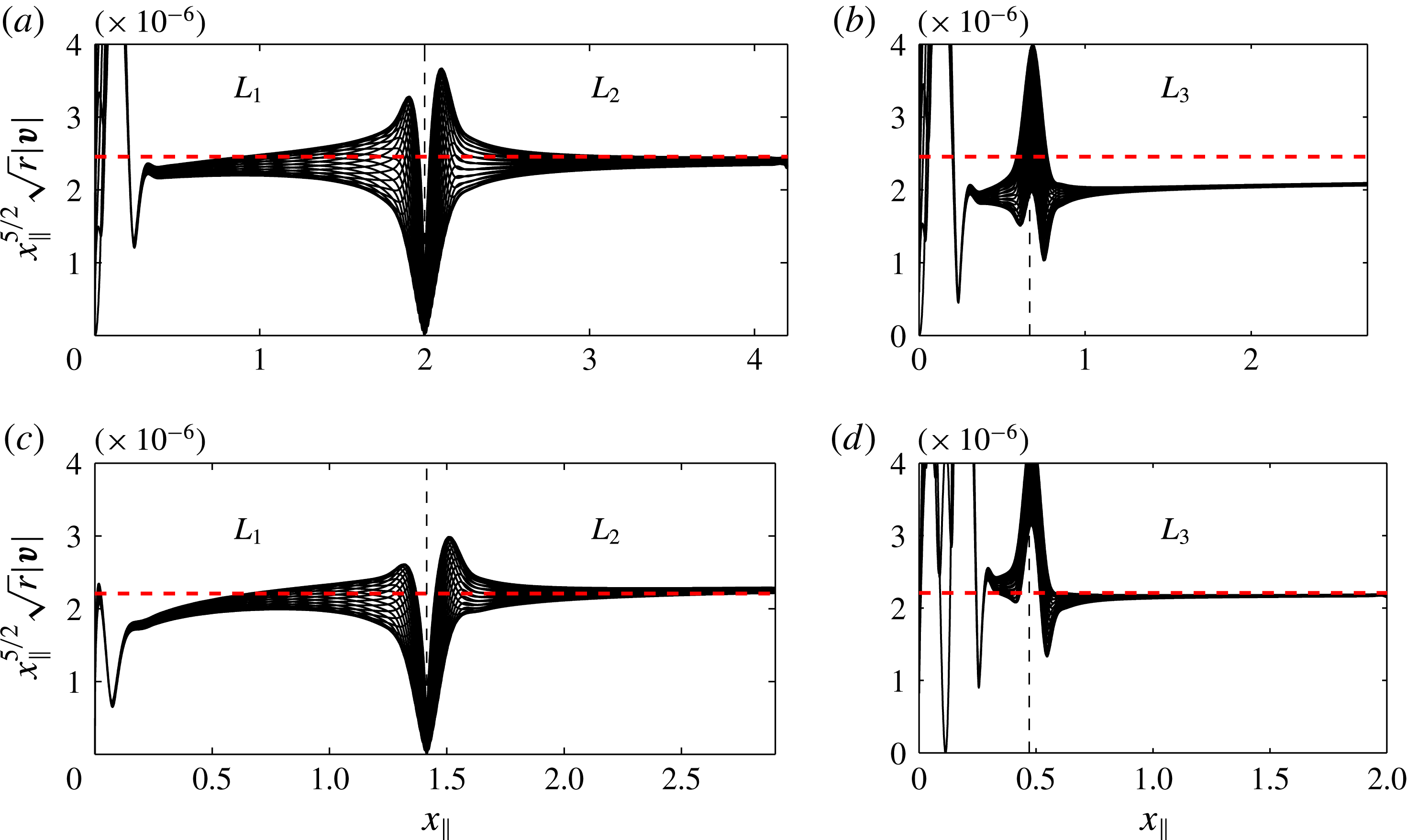
 $|x_{\Vert }|^{5/12}\sqrt{r}|\boldsymbol{v}|$
to remain constant and uniform and given by
 $$\begin{eqnarray}|x_{\Vert }|^{5/12}\sqrt{r}|\boldsymbol{v}|\sim \unicode[STIX]{x1D700}|h_{5/4}(0)|\,|C_{0}|(2\sin \unicode[STIX]{x1D703}_{c})^{5/12}\approx 0.0776\frac{\unicode[STIX]{x1D700}E^{1/12}}{(\sin \unicode[STIX]{x1D703}_{c})^{1/12}|\unicode[STIX]{x1D705}_{c}|^{1/4}}.\end{eqnarray}$$
This is verified in figure 10 where we have plotted
 $|x_{\Vert }|^{5/12}\sqrt{r}|\boldsymbol{v}|$
versus
 $x_{\Vert }$
along the lines
 $L_{1}$
and
 $L_{2}$
(a) and
 $L_{4}$
and
 $L_{3}$
(b) for 25 equidistant times within a period. The theoretical prediction (4.24) is indicated as a red dashed line. The agreement is good for the upper lines
 $L_{1}$
and
 $L_{2}$
. However, as for the disk, there is a weak discrepancy between the theory and the numerics for the constant on the lower lines
 $L_{4}$
and
 $L_{3}$
. Close to
 $x_{\Vert }\approx \sqrt{2}$
, the departures are associated with the impact of
 $L_{1}$
and
 $L_{2}$
on the axis, and with the crossing of
 $L_{4}$
and
 $L_{3}$
.
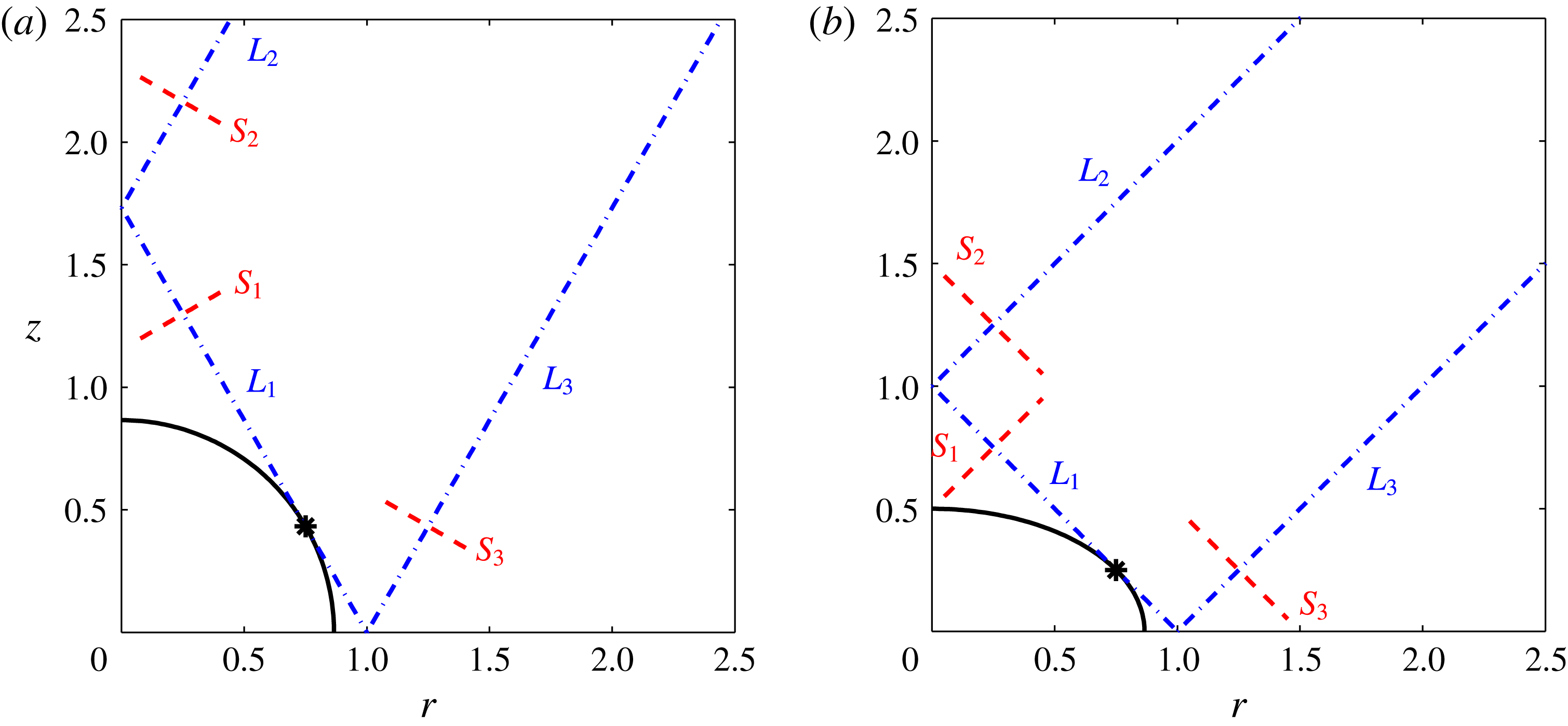
Definition of the characteristic lines and sections for a librating spheroid. (a) Sphere of radius
 $\sqrt{3}/2$
for
 $\unicode[STIX]{x1D714}=1$
. (b) Oblate spheroid of eccentricity
 $\sqrt{2/3}$
for
 $\unicode[STIX]{x1D714}=\sqrt{2}$
.

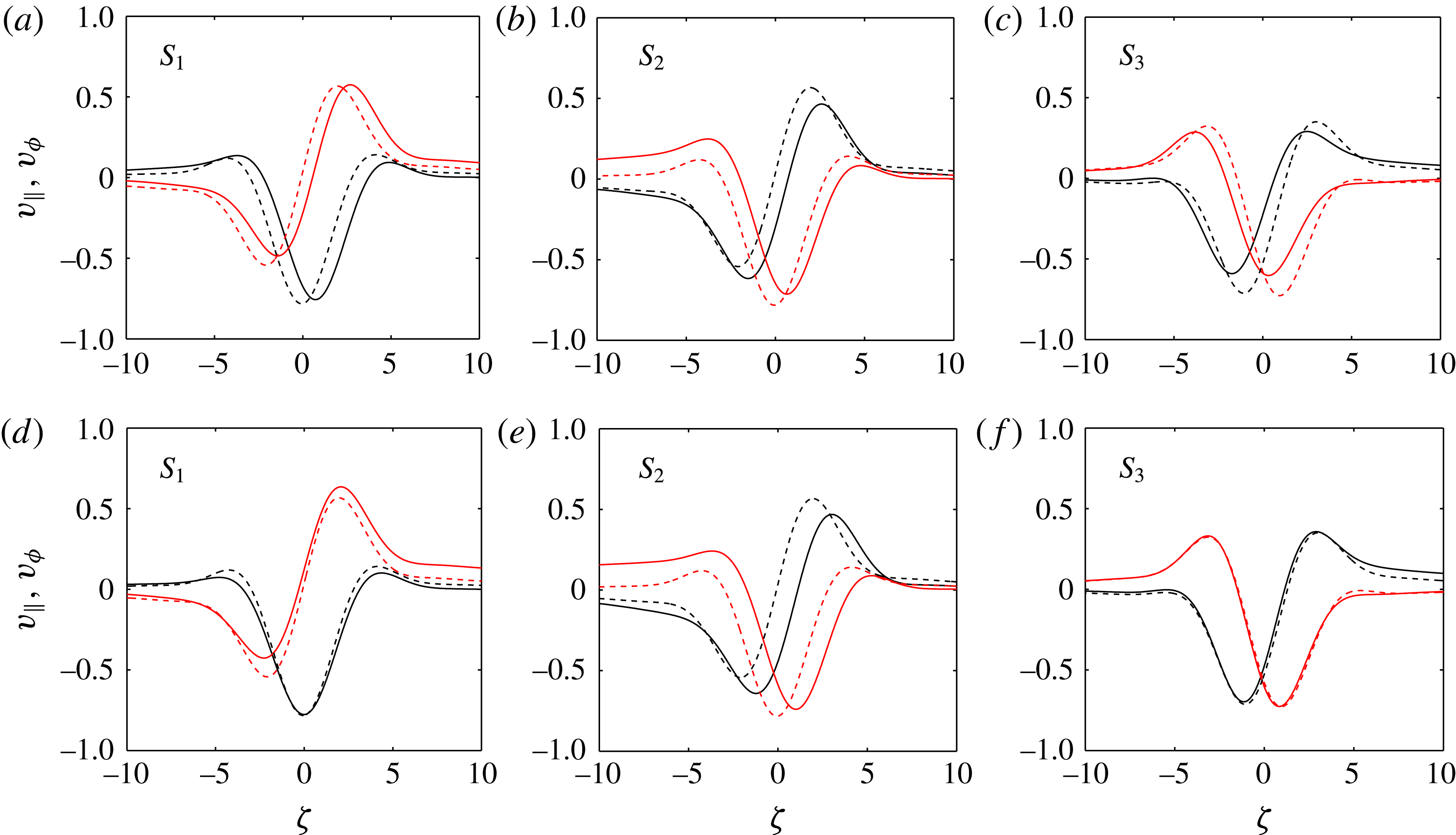
Other geometries have been tested numerically. We present here two other configurations, a sphere with a different frequency and an oblate spheroid (see figure 11). For both cases, we have performed the same tests. In figure 12, we provide plots of
 $v_{\unicode[STIX]{x1D719}}$
and
 $v_{\Vert }$
in different sections indicated in figure 11 using the same normalization as above such that formulas (4.22) still apply. In figure 13, we have plotted as in figure 10, the quantity
 $|x_{\Vert }|^{5/12}\sqrt{r}|\boldsymbol{v}|$
versus
 $x_{\Vert }$
, which is still expected to be provided by (4.24). As previously, we do observe a good agreement between theoretical predictions and numerical results.
Same as figure 9 across the sections defined in figure 11. (a–c) Sphere with
 $\unicode[STIX]{x1D714}=1$
; (d–f) oblate spheroid of eccentricity
 $\sqrt{2/3}$
with
 $\unicode[STIX]{x1D714}=\sqrt{2}$
. For both cases,
 $\unicode[STIX]{x1D700}=10^{-4}$
,
 $E_{s}=10^{-5}$
(i.e.
 $E=1.78\times 10^{-5}$
) and
 $t=508.9\unicode[STIX]{x03C0}/\unicode[STIX]{x1D714}$
.

Same as figure 10 for the configurations defined in figure 11. (a,b) Sphere with
 $\unicode[STIX]{x1D714}=1$
; (c,d) oblate spheroid of eccentricity
 $\sqrt{2/3}$
with
 $\unicode[STIX]{x1D714}=\sqrt{2}$
. For both cases,
 $\unicode[STIX]{x1D700}=10^{-4}$
and
 $E_{s}=10^{-5}$
(i.e.
 $E=1.78\times 10^{-5}$
).

5 Discussion
We have shown that the internal shear layers created by the libration of a convex object can be described by the similarity solutions introduced by Moore & Saffman (Reference Moore and Saffman1969). We have provided the amplitude and the parameter controlling the form of the solution for a disk and for any smooth object. For a smooth object, we have in particular shown that the amplitude is proportional to the local curvature radius at the power
 $1/4$
at the critical latitude where the internal shear layers are emitted. Interestingly, we have also obtained that this amplitude is larger for a smooth object (with a scaling in
 $E^{1/12}$
) than for a disk (with a scaling in
 $E^{1/6}$
). The consequence of this larger amplitude in the internal shear layers is an even larger amplitude in
 $E^{-1/12}$
at the point of focus on the axis (see appendix A). At this particular point on the axis, the solution therefore grows and diverges as
 $E\rightarrow 0$
, clearly demonstrating the singular character of the solution in this limit.
The scaling in
 $E^{1/12}$
for the velocity amplitude in the internal shear layers is larger than that reported in the literature (e.g. Kerswell Reference Kerswell1995; Calkins et al.
Reference Calkins, Noir, Eldredge and Aurnou2010). As a consequence, the zonal flow created by the self-interaction of the harmonic solution is also expected to be larger. Following the analysis performed in Le Dizès (Reference Le Dizès2015), we can expect a zonal flow in
 $\unicode[STIX]{x1D700}^{2}E^{1/6}$
in the internal shear layers and in
 $\unicode[STIX]{x1D700}^{2}E^{-1/2}$
at the focus point on the axis. This last scaling implies that the nonlinear corrections become large as soon as
 $\unicode[STIX]{x1D700}$
reaches
 $E^{1/4}$
, that is well before the linear solution has reached an amplitude of order 1.
For illustrating the geophysical relevance of our results, let us consider two examples: the liquid core of Mercury and the subsurface ocean of Enceladus, whose existences have been demonstrated by studies of their surface librating motions (Margot et al.
Reference Margot, Peale, Jurgens, Slade and Holin2007; Thomas et al.
Reference Thomas, Tajeddine, Tiscareno, Burns, Joseph, Loredo, Helfenstein and Porco2016). Relevant physical parameters are listed in table 1. Using our scaling law (4.24), typical velocities within internal shear layers are
 $1.3\times 10^{-6}$
and
 $1.6\times 10^{-4}~\text{m}~\text{s}^{-1}$
, while estimates for the zonal flow at the focus point give
 $2.0\times 10^{-2}$
and
 $6.3~\text{m}~\text{s}^{-1}$
. For comparison, typical velocities in the Earth’s core related to the convective dynamo are
 $10^{-4}~\text{m}~\text{s}^{-1}$
(Gubbins & Roberts Reference Gubbins and Roberts1987) and typical tidal speeds in the Earth’s oceans are
 $3\times 10^{-2}~\text{m}~\text{s}^{-1}$
(St Laurent & Garrett Reference St Laurent and Garrett2002). The influence of the fluid motions described here on planetary dynamics, for instance through magnetic field generation and energy dissipation, should thus be taken into account.
Physical parameters for the librating motion of the liquid core of Mercury (Margot et al.
Reference Margot, Peale, Jurgens, Slade and Holin2007; Noir et al.
Reference Noir, Hemmerlin, Wicht, Baca and Aurnou2009) and the subsurface ocean of Enceladus (Thomas et al.
Reference Thomas, Tajeddine, Tiscareno, Burns, Joseph, Loredo, Helfenstein and Porco2016). In both cases, we consider a typical viscosity
 $\unicode[STIX]{x1D708}=10^{-6}~\text{m}^{2}~\text{s}^{-1}$
, which is supposedly representative of both water/salty water in oceans and liquid iron in planetary cores (see e.g. de Wijs et al.
Reference de Wijs, Kresse, Vocadlo and Dobson1998).

We have only considered internal shear layers created by libration of an axisymmetric object, hence created by viscous coupling. This forcing is weak as it is actually associated with an oscillating Ekman pumping of order
 $E^{1/2}$
. A larger forcing is obtained when it is generated by pressure forces. For example, if the object was oscillated vertically or horizontally, or when the librating object is non-axisymmetric, as in tidally deformed planetary bodies, a much larger amplitude would have been obtained. This situation has been analysed in several works in the context of stratified fluids (e.g. Mowbray & Rarity Reference Mowbray and Rarity1967). In these cases, internal shear layers have also been observed and described by the same family of similarity solutions in the far field (e.g. Thomas & Stevenson Reference Thomas and Stevenson1972; Hurley & Keady Reference Hurley and Keady1997; Flynn, Onu & Sutherland Reference Flynn, Onu and Sutherland2003; Voisin Reference Voisin2003). It would be interesting to determine whether the present approach can be also used to characterize the near field.
It is finally worth emphasizing that we have considered an open domain only. In a closed geometry such as a spherical shell, the internal shear layers are reflected on the boundaries. This implies that they can interact with themselves after a finite number of reflections modifying their internal structure. Such a modification was already quantified a long time ago for the stationary flow generated between two differentially rotating spheres by Stewartson (Reference Stewartson1966), who showed that the structure of the internal shear layer becomes more complex with nested regions of widths
 $E^{1/3}$
,
 $E^{2/7}$
and
 $E^{1/4}$
. We can imagine that similar complications would occur for the librating case if the internal shear layer would form a closed circuit.
Acknowledgements
This work received support from the French Agence Nationale de la Recherche under the A*MIDEX grant ANR-11-IDEX-0001-02, the LABEX MEC project ANR-11-LABX-0092 and the ANR LIPSTIC project ANR-13-JS05-0004-01.
Appendix A. Local asymptotic solution for the internal shear layer close to the axis
The similarity solution diverges as
 $r$
goes to zero. A new expression has to be obtained close to the axis. For this purpose, we can use the general expression in terms of the Hankel transform
 $$\begin{eqnarray}\displaystyle & \displaystyle v_{r}=\int _{0}^{\infty }U(k)\text{J}_{1}(kr)\text{e}^{\text{i}\unicode[STIX]{x1D707}_{1}z}\,\text{d}k, & \displaystyle\end{eqnarray}$$
 $$\begin{eqnarray}\displaystyle & \displaystyle v_{\unicode[STIX]{x1D719}}=\int _{0}^{\infty }V(k)\text{J}_{1}(kr)\text{e}^{\text{i}\unicode[STIX]{x1D707}_{1}z}\,\text{d}k, & \displaystyle\end{eqnarray}$$
 $$\begin{eqnarray}\displaystyle & \displaystyle v_{z}=\int _{0}^{\infty }W(k)\text{J}_{0}(kr)\text{e}^{\text{i}\unicode[STIX]{x1D707}_{1}z}\,\text{d}k, & \displaystyle\end{eqnarray}$$
 $$\begin{eqnarray}\displaystyle & \displaystyle p=\int _{0}^{\infty }P(k)\text{J}_{0}(kr)\text{e}^{\text{i}\unicode[STIX]{x1D707}_{1}z}\,\text{d}k, & \displaystyle\end{eqnarray}$$
 $\unicode[STIX]{x1D707}_{1}$
is the ‘non-viscous’ wavenumber, which expands, when
 $E\rightarrow 0$
, as
 $$\begin{eqnarray}\unicode[STIX]{x1D707}_{1}\sim k\frac{\cos \unicode[STIX]{x1D703}_{c}}{\sin \unicode[STIX]{x1D703}_{c}}\left(1+\text{i}E\frac{k^{2}}{2\cos \unicode[STIX]{x1D703}_{c}\sin ^{4}\unicode[STIX]{x1D703}_{c}}\right).\end{eqnarray}$$
At leading order, the amplitudes
 $U$
,
 $V$
,
 $W$
and
 $P$
are related with each other by the relations (see Le Dizès Reference Le Dizès2015)
 $$\begin{eqnarray}\displaystyle & \displaystyle W=\text{i}\frac{\sin \unicode[STIX]{x1D703}_{c}}{\cos \unicode[STIX]{x1D703}_{c}}U, & \displaystyle\end{eqnarray}$$
 $$\begin{eqnarray}\displaystyle & U=\text{i}\cos \unicode[STIX]{x1D703}_{c}V, & \displaystyle\end{eqnarray}$$
 $$\begin{eqnarray}\displaystyle & kP=-2V-2\text{i}\cos \unicode[STIX]{x1D703}_{c}U=-2\sin \unicode[STIX]{x1D703}_{c}V. & \displaystyle\end{eqnarray}$$
Introducing the local variables
 $$\begin{eqnarray}\tilde{r}=r/E^{1/3},\quad \tilde{z}=(z-\sin \unicode[STIX]{x1D703}_{c})/E^{1/3},\end{eqnarray}$$
 $$\begin{eqnarray}\displaystyle & \displaystyle v_{r}=\text{i}\cos \unicode[STIX]{x1D703}_{c}\int _{0}^{\infty }\tilde{V}\text{J}_{1}(\tilde{k}\tilde{r})\text{e}^{\text{i}\tilde{k}\,\text{cotan}\,\unicode[STIX]{x1D703}_{c}\tilde{z}}\,\text{d}\tilde{k}, & \displaystyle\end{eqnarray}$$
 $$\begin{eqnarray}\displaystyle & \displaystyle v_{\unicode[STIX]{x1D719}}=\int _{0}^{\infty }\tilde{V}\text{J}_{1}(\tilde{k}\tilde{r})\text{e}^{\text{i}\tilde{k}\,\text{cotan}\,\unicode[STIX]{x1D703}_{c}\tilde{z}}\,\text{d}\tilde{k}, & \displaystyle\end{eqnarray}$$
 $$\begin{eqnarray}\displaystyle & \displaystyle v_{z}=-\sin \,\unicode[STIX]{x1D703}_{c}\int _{0}^{\infty }\tilde{V}\text{J}_{0}(\tilde{k}\tilde{r})\text{e}^{\text{i}\tilde{k}\,\text{cotan}\,\unicode[STIX]{x1D703}_{c}\tilde{z}}\,\text{d}\tilde{k}, & \displaystyle\end{eqnarray}$$
 $$\begin{eqnarray}\displaystyle & \displaystyle p=-2\sin \unicode[STIX]{x1D703}_{c}E^{1/3}\int _{0}^{\infty }\tilde{V}\frac{\text{J}_{0}(\tilde{k}\tilde{r})}{\tilde{k}}\text{e}^{\text{i}\tilde{k}\,\text{cotan}\,\unicode[STIX]{x1D703}_{c}\tilde{z}}\,\text{d}\tilde{k}. & \displaystyle\end{eqnarray}$$
The expression of
 $\tilde{V}$
is obtained by matching these expressions with the similarity solution on
 $L_{1}$
. When both
 $\tilde{z}$
and
 $\tilde{r}$
go to infinity, equation (A 5b
) for
 $v_{\unicode[STIX]{x1D719}}$
can be written as
 $$\begin{eqnarray}v_{\unicode[STIX]{x1D719}}\sim \sqrt{\frac{1}{2\unicode[STIX]{x03C0}\tilde{r}}}\int _{0}^{\infty }\frac{\tilde{V}}{\sqrt{\tilde{k}}}(\text{e}^{\text{i}\tilde{k}(\tilde{r}+\text{cotan}\,\unicode[STIX]{x1D703}_{c}\tilde{z})-3\text{i}\unicode[STIX]{x03C0}/4}+\text{e}^{\text{i}\tilde{k}(-\tilde{r}+\text{cotan}\,\unicode[STIX]{x1D703}_{c}\tilde{z})+3\text{i}\unicode[STIX]{x03C0}/4})\,\text{d}\tilde{k},\end{eqnarray}$$
using the expansion of the Bessel function
 $\text{J}_{1}$
at infinity. If we now assume that
 $$\begin{eqnarray}\tilde{V}=E^{-1/6}C_{0}\frac{\sqrt{2\unicode[STIX]{x03C0}}\tilde{k}^{m-1/2}}{(m-1)!\sin ^{m}\unicode[STIX]{x1D703}_{c}}\text{e}^{-\tilde{k}^{3}/(2\cos \unicode[STIX]{x1D703}_{c}\sin ^{4}\unicode[STIX]{x1D703}_{c})}\text{e}^{5\text{i}\unicode[STIX]{x03C0}/4-\text{i}m\unicode[STIX]{x03C0}/2},\end{eqnarray}$$
this expression becomes
 $$\begin{eqnarray}v_{\unicode[STIX]{x1D719}}\sim \frac{1}{\sqrt{r}}(\text{i}C_{0}H_{m}(1/\cos \unicode[STIX]{x1D703}_{c},\unicode[STIX]{x1D701}^{(1)})+C_{0}H_{m}(1/\cos \unicode[STIX]{x1D703}_{c},\unicode[STIX]{x1D701}^{(2)})),\end{eqnarray}$$
where
 $\unicode[STIX]{x1D701}^{(1)}$
and
 $\unicode[STIX]{x1D701}^{(2)}$
are the similarity variables close to the axis along
 $L_{1}$
and
 $L_{2}$
respectively:
 $$\begin{eqnarray}\displaystyle & \unicode[STIX]{x1D701}^{(1)}=(2\sin \unicode[STIX]{x1D703}_{c}\cos \unicode[STIX]{x1D703}_{c})^{1/3}(\sin \unicode[STIX]{x1D703}_{c}\tilde{r}+\cos \unicode[STIX]{x1D703}_{c}\tilde{z}), & \displaystyle\end{eqnarray}$$
 $$\begin{eqnarray}\displaystyle & \unicode[STIX]{x1D701}^{(2)}=(2\sin \unicode[STIX]{x1D703}_{c}\cos \unicode[STIX]{x1D703}_{c})^{1/3}(-\sin \,\unicode[STIX]{x1D703}_{c}\tilde{r}+\cos \unicode[STIX]{x1D703}_{c}\tilde{z}). & \displaystyle\end{eqnarray}$$
The first term in (A 8) is exactly the expression of the azimuthal velocity component of the similarity solution along
 $L_{1}$
close to
 $x_{\Vert }=1/\cos \unicode[STIX]{x1D703}_{c}$
(see expressions (2.8) and (2.15)). The second term corresponds to the similarity solution along
 $L_{2}$
. It shows that the azimuthal velocity component of the similarity solution keeps the same amplitude but with a phase shift of
 $-\unicode[STIX]{x03C0}/2$
. Along
 $L_{2}$
, the expressions (2.10) and (2.15) for
 $v_{\Vert }^{(0)}$
and
 $v_{\unicode[STIX]{x1D719}}^{(0)}$
have thus to be replaced by
 $$\begin{eqnarray}v_{\Vert }^{(0)}=\text{i}C_{0}H_{m}(x_{\Vert },\unicode[STIX]{x1D701}),\quad v_{\unicode[STIX]{x1D719}}^{(0)}=C_{0}H_{m}(x_{\Vert },\unicode[STIX]{x1D701}),\end{eqnarray}$$
where
 $x_{\Vert }$
starts at the value
 $1/\cos \unicode[STIX]{x1D703}_{c}$
from the point
 $(0,\tan \unicode[STIX]{x1D703}_{c})$
on the
 $z$
axis.
In the
 $O(E^{1/3})$
neighbourhood around the focus point, the solution is given by (A 5a
–
d
) with
 $\tilde{V}$
and
 $C_{0}$
provided by (A 7) and (4.20b
), respectively. In particular, this implies that the three velocity components become of order
 $E^{-1/12}$
close to the focus point.